Artificial Intelligence

Constraint Satisfaction Problems

Marc ToussaintUniversity of StuttgartWinter 2015/16

(slides based on Stuart Russell’s AI course)

Inference

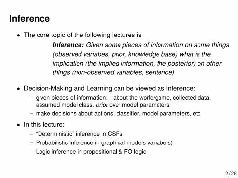
• The core topic of the following lectures is

Inference: Given some pieces of information on some things(observed variabes, prior, knowledge base) what is theimplication (the implied information, the posterior) on otherthings (non-observed variables, sentence)

• Decision-Making and Learning can be viewed as Inference:– given pieces of information: about the world/game, collected data,

assumed model class, prior over model parameters– make decisions about actions, classifier, model parameters, etc

• In this lecture:– “Deterministic” inference in CSPs– Probabilistic inference in graphical models variabels)– Logic inference in propositional & FO logic

2/28

ontrees

CSP

graphicalmodelsMDPs

sequentialdecisionproblems

searchBFS

propositionallogic FOL

relationalgraphicalmodels

relationalMDPs

ReinforcementLearning

HMMs

ML

multi-agentMDPs

MCTS

utilities

dete

rmin

isti

cle

arn

ing

pro

babili

stic

propositional relationalsequentialdecisions

games

banditsUCB

constraintpropagation

beliefpropagationmsg. passing

ActiveLearning

Deci

sion T

heory dynamic

programmingV(s), Q(s,a)

fwd/bwdchaining

backtracking

fwd/bwdmsg. passing

FOL

sequential assignment

alpha/betapruning

minimax

3/28

Constraint satisfaction problems (CSPs)

• In previous lectures we considered sequential decision problemsCSPs are not sequential decision problems. However, the basicmethods address them by testing sequentially ’decisions’

• CSP:– We have n variables xi, each with domain Di, xi ∈ Di

– We have K constraints Ck, each of which determines the feasibleconfigurations of a subset of variables

– The goal is to find a configuration X = (X1, .., Xn) of all variables thatsatisfies all constraints

• Formally Ck = (Ik, ck) where Ik ⊆ {1, .., n} determines the subset ofvariables, and ck : DIk → {0, 1} determines whether a configurationxIk ∈ DIk of this subset of variables is feasible

4/28

Example: Map-Coloring

Variables W , N , Q, E, V , S, T (E = New South Wales)Domains Di = {red, green, blue} for all variablesConstraints: adjacent regions must have different colors

e.g., W 6= N , or(W,N) ∈ {(red, green), (red, blue), (green, red), (green, blue), . . .}

5/28

Example: Map-Coloring contd.

Solutions are assignments satisfying all constraints, e.g.,{W = red,N = green,Q= red,E= green, V = red, S= blue, T = green}

6/28

Constraint graph

• Pair-wise CSP: each constraint relates at most two variables

• Constraint graph: a bi-partite graph: nodes are variables, boxes areconstraints

• In general, constraints may constrain several (or one) variables(|Ik| 6= 2)

c1

c2

c3

c6c8

c4c5

c7

T

V

E

QN

S

W c9

7/28

Varieties of CSPs

• Discrete variables: finite domains; each Di of size |Di| = d ⇒ O(dn)

complete assignments– e.g., Boolean CSPs, incl. Boolean satisfiability infinite domains (integers,

strings, etc.)– e.g., job scheduling, variables are start/end days for each job– linear constraints solvable, nonlinear undecidable

• Continuous variables– e.g., start/end times for Hubble Telescope observations– linear constraints solvable in poly time by LP methods

• Real-world examples– Assignment problems, e.g. who teaches what class?– Timetabling problems, e.g. which class is offered when and where?– Hardware configuration– Transportation/Factory scheduling

8/28

Varieties of constraintsUnary constraints involve a single variable, |Ik| = 1

e.g., S 6= green

Pair-wise constraints involve pairs of variables, |Ik| = 2

e.g., S 6= W

Higher-order constraints involve 3 or more variables, |Ik| > 2

e.g., Sudoku

9/28

Methods for solving CSPs

10/28

Sequential assignment approachLet’s start with the straightforward, dumb approach, then fix itStates are defined by the values assigned so far

• Initial state: the empty assignment, { }• Successor function: assign a value to an unassigned variable that does

not conflict with current assignment ⇒ fail if no feasible assignments(not fixable!)

• Goal test: the current assignment is complete

1) Every solution appears at depth n with n variables ⇒ usedepth-first search2) b=(n− `)d at depth `, hence n!dn leaves!

11/28

Backtracking sequential assignment

• Two variable assignment decisions are commutative, i.e.,[W = red then N = green] same as [N = green then W = red]

• We can fix a single next variable to assign a value to at each node

• This does not compromise completeness (ability to find the solution)⇒ b= d and there are dn leaves

• Depth-first search for CSPs with single-variable assignmentsis called backtracking search

• Backtracking search is the basic uninformed algorithm for CSPs

Can solve n-queens for n ≈ 25

12/28

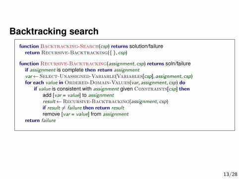
Backtracking searchfunction Backtracking-Search(csp) returns solution/failure

return Recursive-Backtracking({ }, csp)

function Recursive-Backtracking(assignment, csp) returns soln/failureif assignment is complete then return assignmentvar←Select-Unassigned-Variable(Variables[csp],assignment, csp)for each value in Ordered-Domain-Values(var,assignment, csp) do

if value is consistent with assignment given Constraints[csp] thenadd [var = value] to assignmentresult←Recursive-Backtracking(assignment, csp)if result 6= failure then return resultremove [var = value] from assignment

return failure

13/28

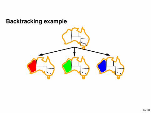
Backtracking example

14/28

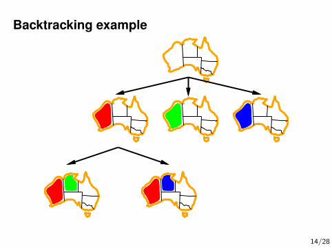
Backtracking example

14/28

Backtracking example

14/28

Backtracking example

14/28

Improving backtracking efficiencySimple heuristics can give huge gains in speed:

1. Which variable should be assigned next?2. In what order should its values be tried?3. Can we detect inevitable failure early?4. Can we take advantage of problem structure?

15/28

Minimum remaining valuesMinimum remaining values (MRV):

choose the variable with the fewest legal values

16/28

Degree heuristicTie-breaker among MRV variablesDegree heuristic:

choose the variable with the most constraints on remaining variables

17/28

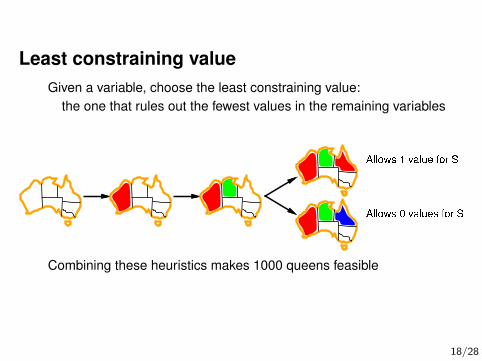
Least constraining valueGiven a variable, choose the least constraining value:

the one that rules out the fewest values in the remaining variables

Combining these heuristics makes 1000 queens feasible

18/28

Constraint propagation

• After each decision (assigning a value to one variable) we can computewhat are the remaining feasible values for all other variables.

• Initially, every variable has the full domain Di. Constraint propagationreduces these domains, deleting entries that are inconsistent with thenew decision.These dependencies are recursive: Deleting a value from the domainof one variable might imply infeasibility of some value of anothervariable→ contraint propagation. We update domains until they’re allconsistent with the constraints.

This is Inference

19/28

Constraint propagation

• Example of just “1-step propagation”:

N and S cannot both be blue!Idea: propagate the implied constraints serveral steps further

Generally, this is called constraint propagation

20/28

Arc consistency (=constraint propagation forpair-wise constraints)

Simplest form of propagation makes each arc consistentX → Y is consistent iff

for every value x of X there is some allowed y

If X loses a value, neighbors of X need to be recheckedIf X loses a value, neighbors of X need to be recheckedArc consistency detects failure earlier than forward checkingCan be run as a preprocessor or after each assignment

21/28

Arc consistency (=constraint propagation forpair-wise constraints)

Simplest form of propagation makes each arc consistentX → Y is consistent iff

for every value x of X there is some allowed y

If X loses a value, neighbors of X need to be recheckedIf X loses a value, neighbors of X need to be recheckedArc consistency detects failure earlier than forward checkingCan be run as a preprocessor or after each assignment

21/28

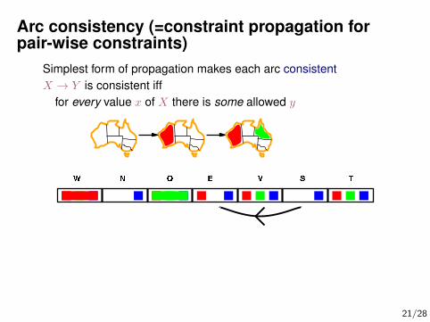
Arc consistency (=constraint propagation forpair-wise constraints)

Simplest form of propagation makes each arc consistentX → Y is consistent iff

for every value x of X there is some allowed y

If X loses a value, neighbors of X need to be rechecked

If X loses a value, neighbors of X need to be recheckedArc consistency detects failure earlier than forward checkingCan be run as a preprocessor or after each assignment

21/28

Arc consistency (=constraint propagation forpair-wise constraints)

Simplest form of propagation makes each arc consistentX → Y is consistent iff

for every value x of X there is some allowed y

If X loses a value, neighbors of X need to be rechecked

If X loses a value, neighbors of X need to be recheckedArc consistency detects failure earlier than forward checkingCan be run as a preprocessor or after each assignment

21/28

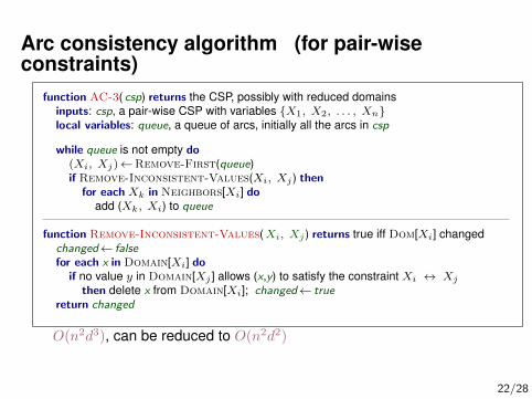
Arc consistency algorithm (for pair-wiseconstraints)

function AC-3( csp) returns the CSP, possibly with reduced domainsinputs: csp, a pair-wise CSP with variables {X1, X2, . . . , Xn}local variables: queue, a queue of arcs, initially all the arcs in csp

while queue is not empty do(Xi, Xj)←Remove-First(queue)if Remove-Inconsistent-Values(Xi, Xj ) then

for each Xk in Neighbors[Xi] doadd (Xk, Xi) to queue

function Remove-Inconsistent-Values(Xi, Xj ) returns true iff Dom[Xi] changedchanged← falsefor each x in Domain[Xi] do

if no value y in Domain[Xj ] allows (x,y) to satisfy the constraint Xi ↔ Xj

then delete x from Domain[Xi]; changed← truereturn changed

O(n2d3), can be reduced to O(n2d2)

22/28

Constraint propagationSee textbook for details for non-pair-wise constraintsVery closely related to message passing in probabilistic models

In practice: design approximate constraint propagation for specificproblem

E.g.: Sudoku: If Xi is assigned, delete this value from all peers

23/28

Problem structure

c1

c2

c3

c6c8

c4c5

c7

T

V

E

QN

S

W c9

Tasmania and mainland are independent subproblemsIdentifiable as connected components of constraint graph

24/28

Tree-structured CSPs

Theorem: if the constraint graph has no loops, the CSP can be solvedin O(nd2) timeCompare to general CSPs, where worst-case time is O(dn)

This property also applies to logical and probabilistic reasoning!

25/28

Algorithm for tree-structured CSPs

1. Choose a variable as root, order variables from root to leavessuch that every node’s parent precedes it in the ordering

2. For j from n down to 2, applyRemoveInconsistent(Parent(Xj), Xj)

This is backward constraint propagation

3. For j from 1 to n, assign Xj consistently with Parent(Xj)

This is forward sequential assignment (trivial backtracking)

26/28

Nearly tree-structured CSPsConditioning: instantiate a variable, prune its neighbors’ domains

Cutset conditioning: instantiate (in all ways) a set of variablessuch that the remaining constraint graph is a treeCutset size c ⇒ runtime O(dc · (n− c)d2), very fast for small c

27/28

Summary

• CSPs are a fundamental kind of problem:finding a feasible configuration of n variablesthe set of constraints defines the (graph) structure of the problem

• Sequential assignment approachBacktracking = depth-first search with one variable assigned per

node

• Variable ordering and value selection heuristics help significantly

• Constraint propagation (e.g., arc consistency) does additional work toconstrain values and detect inconsistencies

• The CSP representation allows analysis of problem structure

• Tree-structured CSPs can be solved in linear timeIf after assigning some variables, the remaining structure is a tree→ linear time feasibility check by tree CSP

28/28