Artifact and noise stripping on low-field brain MRI · Abstract—Low-field Magnetic Resonance...

Abstract—Low-field Magnetic Resonance Imaging (MRI) is a

relatively new technology that is used in operating rooms to allow

real-time imaging. The images produced are valuable for guidance

and assessment during the surgery, but the low signal strength

produces very low resolution images with noise and artifacts. This

study shows that implementation of a dynamic pre-processing

algorithm to extract the brain region in low-field MRI images is

crucial in order to accurately segment the brain image. Conceptually,

histogram-based analysis indicates that most low-field MR images

consist of three peaks, where the first and second peaks summarize

the background and artifacts, respectively, while the third peak is the

region-of-interest (ROI). This paper provides some useful insight of

steps that could be taken prior to brain segmentation. Promising

results are reported for both qualitative and quantitative

measurements.

Keywords— Dynamic thresholding, Histogram analysis, Image

enhancement, Magnetic Resonance Imaging (MRI), Normalization.

I. INTRODUCTION

MAGE processing techniques make it possible to extract

meaningful information from medical images. Brain

Magnetic Resonance Imaging (MRI) images provide

information of brain parts such as white matter (WM), gray

matter (GM), cerebrospinal fluid (CSF), ventricles, skull and

injuries such as bleeding, cyst, tumor and skull fracture. Low-

field MRI is vital for sensitive surgery to allow real-time

imaging in the operation theatre. An open low-field system

would have a number of advantages over its conventional

counterpart, including low-cost, reduced MR compatibility

demands on instruments to minimize distortion, reduced fringe

fields and the relative ease of movement and usage. The main

problem with low-field MRI is its low resolution images. To

achieve the best result in diagnosing disease, medical images

must have good quality and be free from noise and artifacts.

Manuscript received January 9, 2009: This work was supported in part by

the Ministry of Science, Technology and Innovation (MOSTI), Malaysia

under the science fund grant.

N. Faiza Ishak is a Research Officer with the Faculty of Engineering,

Multimedia University, 63100 Cyberjaya, Selangor, Malaysia (Phone: +603-

8312-5258; fax: +603-8318-3029; e-mail: [email protected]).

R. Logeswaran is a Senior Lecturer with the Faculty of Engineering,

Multimedia University, 63100 Cyberjaya, Selangor, Malaysia (e-mail:

[email protected]).

W.H. Tan is a lecturer with the Faculty of Engineering, Multimedia

University, 63100 Cyberjaya, Selangor, Malaysia (e-mail:

[email protected]).

Brain stripping is used to classify head image elements into

two rigid classes, brain and non-brain [1]. It should be noted

that a simple segmentation scheme used on conventional MRI

images is a priori not sufficient to solve the problem. In

additional, Gribkov [2] proposed a few segmentation methods

on low contrast images and segmentation of domains with

varying intensity. Fig. 1 shows the flowchart for typical brain

segmentation which consists of 5 steps [3].

Fig. 1. Flowchart of complete brain segmentation on low-field MRI brain

The first step is to identify anatomical areas of interest in

order to diagnose diseases and injuries. Usually this is done by

the medical experts or radiologist in the hospital. Pre-

processing techniques will be applied next for image

enhancement. Since low-field brain MRI produces low

resolution images, this step is crucial in making the region-of-

interest (ROI) to appear clearer and noise-free. Once the pre-

processing step is completed, feature extraction will be applied

Artifact and noise stripping on low-field brain

MRI

Nur Faiza Ishak, Rajasvaran Logeswaran, Wooi-Haw Tan

I

Identify/ evaluate anatomical

areas of interest

Pre-process raw image for

enhancement

Feature extraction/ selection/

reduction

(Skull, ventricle, brain tissue)

Brain tissue segmentation

(white matter, gray matter,

cerebrospinal fluid)

Classification & Labeling

INTERNATIONAL JOURNAL OF BIOLOGY AND BIOMEDICAL ENGINEERING

Issue 2, Volume 2, 2008 59

to efficiently specify the boundaries between the brain

structures to be identified, e.g. skull, brain tissues as well as

ventricles. Segmentation will be used to distinguish the regions

corresponding to different tissue types. Finally, the segmented

regions will be labeled accordingly.

This paper proposes a complete pre-processing module

using dynamic thresholding. There has been a lot of research

work on pre-processing techniques [4], image intensity

analysis [5-8] and image normalization [9-11] for conventional

MR images. However, most of the techniques proposed are not

directly applicable to low-field MR images [12]. Hence, an

improved method of pre-processing low-field MR images is

required. The technique should allow the structure of the brain

to be more visible in the low-field MRI images.

In the pre-processing phase, normalization and background

removal will be able to reduce the distortion of gray level and

contrast [13]. A typical pre-processing phase usually consists

of smoothing, edge detection, binarization, noise filtering as

well as image sharpening [14-15]. These techniques are

applicable to medical images as well as common images.

Besides, effective image enhancement for medical diagnosis

should consider the basic human visual properties for more

efficient diagnosis.

The structure of this paper is as follows. The next section

briefly discusses the background of low-field MRI. Section 3

describes the proposed histogram analysis method for low-

field MRI images. The performance assessment is given in

Section 4, which is followed by the conclusion in Section 5.

II. BACKGROUND

What advantages of low-field MRI make it more suitable for

brain surgery? The much simpler magnet setup offers many

advantages: the possibility of using open magnets (minimizes

claustrophobia), less static magnetic field exposure to the

surrounding area, less costly equipment that is well-suited for

the standard operating room (OR) environment, compatible

with the electronic equipment and surgical tools, and relatively

small size that is practical in cramped spaces. Furthermore, in

situations where high-field strengths may drown out subtle

signal differences, the low-field MRI becomes invaluable to

detect these (such as in differentiating cancerous and non-

cancerous tissue [16]).

It is usable in the OR and hence can update images to reflect

the changes in anatomy after opening the skull in neurosurgery

[17]. Furthermore, open low-field MRI is preferable to the

tunnel-style conventional MRI for claustrophobic patients.

Several previous studies have compared conventional MRI

(1.5T) versus low-field MRI (0.15T), with most indicating no

significant clinical differences in interpretations of low-field

versus conventional images [18]. Thus, they are clinically

applicable in operations and even routine checkups.

However, since low-field MRI uses low strength

electromagnetic fields, noisy low resolution images are

produced. In contrast, high-field MRI machines

(approximately 7T) are able to produce clear detailed images

with almost no noise at all. Considering the above, the

motivation to enhance the low-field images is so that the same

conventional and high-field MRI processing techniques and

applications could be applied to the pre-processed low-field

MRI images, allowing it to capitalize on the existing findings

and advances technology.

Histogram analysis has been widely used in medical image

processing. Background rejection is one of the common

methods based on histogram analysis, where approximately

10% of the maximum gray level is eliminated [19]. However,

since the intensity non-uniformity may exist in all directions,

usually the normalization procedure will be repeated for all

directions. Identifying optimal thresholds is always a challenge

in MRI due to the wide variance in inter-patient and inter-

image intensity distributions.

Fig. 2 shows the differences in conventional and low-field

MRI images. Both images were taken from the same patient,

for the same slice of the brain. However, the quality is

noticeably worse in the low-field brain image. Not only is the

noise level increased, but the orientation and coverage of the

brain is affected as well due to the small aperture of the low-

field machine. The lower part of the brain is no longer visible

and an artifact is present at the top left (although not very

visible in this image, it hinders automatic processing).

Fig. 2. Conventional MRI (left) and low-field MRI (right) images

Low-field MRI usually has a gray or black background with

an elliptic artifact. The background should be removed as it is

not part of the brain. This technique has been used in [20] as

one of the pre-processing steps in brain region extraction. In

[19], it was expected that a distinct peak in the histogram exist

for determining the threshold value for the entire image, such

that the image could be properly enhanced. Furthermore, this

technique aims at disconnecting, as much as possible, the brain

from surrounding structures. For instance, the low intensity

eliminates the ventricle while the high intensity will eliminate

the skull. However, this adaptation is difficult to perform

automatically due to the large inter-image contrast variety.

III. HISTOGRAM ANALYSIS

As low-field MRI equipment is still quite rare, a database of

only 14 patients was available in this work. Each 128x128



pixels image was analyzed in terms of its intensity histogram.

The parts of interest in a typical low-field MRI brain image are

labeled in Fig. 3(a), with its histogram given in Fig. 3(b). Any

pre-processing undertaken should preserve all the ROI, which

in this case are the labeled areas excluding the artifact and

background.

(a) Original image

(b) Histogram

Fig. 3. Low-field MRI brain image and histogram

Upon inspection of the histogram, it is found that three

peaks exist. P1, the first peak, is expected to be the

background of the image, while P2 may contain most of the

unwanted artifacts. As such, the object of interest, which is the

brain, should be represented by P3. The fourth peak (P4) exists

at intensity 255 in most images. It is present in Fig. 5(b),

although not obvious. P4, being the highest intensity, is

expected to be parts of the skull and bleeding in the brain.

The objective of image processing of the MRI brain is to

extract the features, more specifically the brain tissue,

ventricle, skull, diseased brain areas and abnormalities. Fig. 4

shows the detailed proposed method for pre-processing the

image. Three main steps are to be taken, namely, background

elimination, artifact elimination and finally image

normalization. Elimination of undesirable regions is crucial in

order to obtain precise segmentation of the brain.

Fig. 4. Flowchart of image pre-processing module

A. Histogram Truncation

To examine the above hypothesis, histogram-based pre-

processing techniques were applied to the image database. The

image was then normalized to enhance its contrast.

Normalization is crucial for the extraction and segmentation of

the ROI for future work. This reduces the dynamic range of

intensities between images, standardizing them and making

them more suitable for subsequent processing.

The process initiates with the elimination of the first peak

(P1), which is expected to be the background. By referring to

the result (Fig. 5(b)) of the sample image in Fig. 5(a), it is

shown that the background of the image is removed once the

P1 has been eliminated. The remaining region is the elliptical

shaped brain with the artifact. This supports the assumption

that the first peak consists mostly of the background and its

truncation eliminates the uncounted image background.

Image Acquisition

Low-field MRI image

Background Elimination

To disregard the image

background

Artifact Elimination

To remove non-brain area

surrounding the ROI

Image Normalization

To standardize the grayscale

range

Pre-processed Image

Ready to be segmented

P2 P3

P1 P4

Artifact

Skull

Background

Ventricle

Brain tissue



The next step is artifact elimination, i.e. the second peak

(P2). By determining the maximum intensity of P2, (1) is used

to choose the intensity range in the elimination technique.

Threshold, T p

P )1min(max(P2) −= (1)

where max(P2) is the maximum intensity value of P2, min(P1)

is minimum intensity of the P1 truncated image (P1), and p is

the fraction of the slope for each thresholding step.

Very small steps (e.g p=1/5) did not produce much

differences between the steps. However, large steps (e.g

p=1/2) may allow unseen regions to go missing during the

process as the step size would be large.

By truncating 1/3 off the second peak of the histogram (i.e.

p=1/3), part of the artifact managed to be reduced as shown in

Fig. 5(c). The ROI remains unaffected with this threshold

value but parts of the artifact remains. Hence, a further 1/3

step elimination (i.e. p=2/3) is carried on. Fig. 5(d) shows that

a significant amount of the artifact has been successfully

removed at this stage. The human brain can be more clearly

identified now as compared to the original image.

Since there are still undesired spots of artifacts in the image,

the whole second peak is removed. Referring to Fig. 5(e), it is

now proven that almost all the visible area of the unwanted

region has now been successfully removed. The important

brain areas such as ventricle, diseased region and brain tissue

are unaffected. The processed image is now more similar to

the conventional MRI images, where the difference between

the brain and the background can be distinguished clearly. The

background and artifact have been completely removed and

will no longer influence any consequent processing techniques

applied to the image.

0 126 255

(a) Original image

0 128 255 0 142 255

(b) P1 eliminated (c) 1/3 of P2 eliminated

0 156 255 0 170 255

(d) 2/3 of P2 eliminated (e) Entire P2 eliminated

0 255

(f) Normalized image

Fig. 5. Histogram truncation and normalization



B. Normalization

Truncating the histogram peaks alone is not sufficient.

Examining the images available, it was observed that the

intensity range of the low-field MRI images are inconsistent

(some in the higher ranges whilst others in the lower ranges).

Thus, image normalization should be applied to the pre-

processed image to standardize the intensity range to 0-255.

By stretching the histogram, the image brightness will be more

uniform. Some parts of the brain that were not clearly visible

would become more obvious after normalization. Eq. (2) is

used to normalize the image,

)12( −×−

−=

Cd

T)TImax(

TTIIimage, Normalized (2)

where IT is thresholded image using threshold T, max(IT) is

maximum intensity of IT, Cd is the color depth (in bpp), e.g.

Cd = 8 sets the grayscale intensity range between 0-255.

Fig. 5(f) shows the resulting histogram of the pre-processed

image in Fig. 5(e), stretched from the range 155-255 to 0-255.

A clearer image is produced and hence leads towards better

identification of the ROI. As an example to illustrate the

enhancement, notice that it is difficult to determine the

boundaries of the bleed area in Fig. 5(e) (the white area near

the middle of the brain). After the image is normalized, the

differences can be seen clearly, without the application of any

further complicated enhancement techniques. This reduces the

time and cost of processing at the subsequent stages.

IV. PERFORMANCE ASSESSMENT

To validate the performance of the proposed pre-processing

technique, tests were conducted on the entire database. The

results achieved by applying the proposed technique on a set

of images with different characteristics are given below. The

characteristics were chosen to compare the accuracy and

robustness of the technique. The assessment performed

encompasses both qualitative and quantitative measurements.

For the assessment, there are a number of criteria that need

to be fulfilled in order to determine the effectiveness and

consistency of the proposed method, in terms of the visibility

of the pre-processed image, i.e. clear detail of the brain tissue,

the existence of three main parts of the brain (skull, ventricle

and brain tissue), as well as a complete elimination of non-

brain area.

A. Visual Comparison

For the basic human visual evaluation, the test was divided

into two categories – normal brain images and brain images

with various diseases/ injuries. The results obtained are given

in Fig. 6 and Fig. 7, respectively.

a) Normal Brain

For all 6 test images of patients with normal brain condition

shown in Fig. 6, the separation between ventricle and white

matter becomes more obvious after pre-processing. The same

goes for the visibility of brain folds (consisting of gray matter).

The artifacts in the original images were also successfully

removed.

(a)

(b)

(c)

(d)

(e)

(f)

Fig. 6. Results of the proposed pre-processing

technique on normal brain



In Fig. 6 (b), (d) and (e), it is obvious that all the details in

the pre-processed image are visible enough for diagnosis,

should there be any diseases. Besides, the properties of the

images themselves, such as orientation, brain coverage and the

clarity of the three main parts of the brain, makes it easier to

evaluate these images.

For the results shown in Fig. 6 (a), (c) and (f), the

orientation of the brain is tilted to the left or right in the

different images. Despite the criteria stated before, the

technique still produces excellent pre-processed image output.

With this, it proves that the performance of the proposed

method is excellent for normal low-field brain MRI images.

b) Diseased Brain

The image database obtained included a number of images

that have been diagnosed with various diseases and injuries,

such as bleeding, cyst, tumor, skull fracture, abnormalities as

well as hydrocephalus of the ventricle. In addition, post-

operation images are also included in this test.

Evaluating all of the images in Fig. 7, approximately 98% of

the artifacts surrounding the brain ROI has been eliminated,

regardless of the orientation of the brain. The output image is

sharper than the original image without the need for further

image sharpening. The details of the brain tissues are more

prominent after the normalization.

Fig. 7(a) is an example of bleeding at the brain tissue

boundaries. As can be seen in the original image, the

separation between skull and bleeding area is less defined.

However, after applying the pre-processing technique, a clear

brain image with well-shaped boundaries between the brain

tissues, bleeding as well as the skull is obtained.

Fig. 7(b) and (c) show more examples of bleeding in the

brain. After image normalization, the brain folds become more

visible. This can lead to a more precise segmentation with less

distortion and noise. Fig. 7(d) shows ventricle abnormalities

where in the original image, it is difficult to determine the

brain folds and the actual brain ROI. The normalized brain

image after the pre-processing phase can be seen clearly as

compared to the original image.

Fig. 7(e) is a post-operation image where the skull has been

separated. Fig. 7(f) is the post-operation brain image for Fig.

7(c). In both cases, the proposed technique has proven to be

successful. In Fig. 7(g) – (k), the images comprise of various

types of brain lesions. Due to the low resolution of the original

images, it is difficult to distinguish the exact boundaries for all

the tumors from the brain tissue as the intensity tends to be

similar.

However, after truncating the unnecessary background

artifact and normalizing the images, an obvious range of

intensity can be observed especially at the boundaries between

the tumors and brain tissue. This step is essential in order to

accurately segment the diseased region for diagnosis As low-

field MRI is used in the operating room to allow real-time

imaging, such pre-processing would assist the surgeon in

clearly distinguish the areas of interest.

The final image seen in Fig. 7(l) is that of a brain associated

with a type of Alzheimer’s disease called hydrocephalus.

However, there is an unknown object detected during the scan.

This type of additional artifact is not removed using the

proposed technique as the object and its intended purpose is

not known. As the object may have been deliberately included,

or may be a vital part in aiding diagnosis, the output achieved

as desired. Since the original image is rather dark, the

histogram was almost equally distributed. There were no

obvious peaks in this low quality image.

By observing all of the images in Fig. 7, the white marked

arrow clearly shows the interested area to be eliminated since

some of the image contrast unable to show the artifact

boundaries. This proves the existence of elliptical shape

aperture during the scanning using the low-field MRI machine.

Thus, the actual brain image does not necessarily covered in

all of the elliptical shape. The medical experts will only scan

the area of interest for the surgery, such as tumor or bleeding

area.

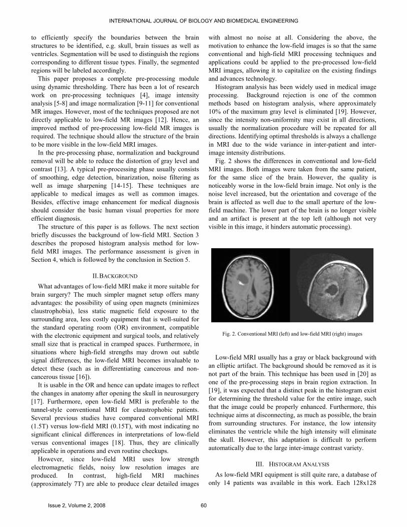
B. Additional Information

An alternative approach after the truncation of P1 is for the

resulting histogram to be shifted to the left (see Fig. 8(a)).

However, as the image becomes dimmer, the artifact is no

longer visually obvious although it is still present and affects

subsequent processing. Nonetheless, the same final result is

obtained once the whole of P2 is removed. As such, either

approach may be used.

In addition, to determine the amount of ROI that has been

removed, subtracting the original image with the pre-processed

image of Fig. 5(d) shows the differences as in Fig. 8(b). As

observed, the whole background was eliminated and only very

small parts of the brain area (see the few pixels in the brain

area in the figure) were affected. This shows that the proposed

technique is effective in eliminating unwanted regions while

preserving the integrity of the areas of importance (i.e. the

brain). The information provided by the image subtraction

could be stored and used when further accuracy is required in

subsequent processing.

C. Comparison of Edge Detection

Finding edges in an image is considered to be an important

process in many artificial vision systems. There are three

criteria that need to be fulfilled for optimal edge detection that

will lead to better segmentation, namely, good localization,

good detection as well as single response constraint which will

return only one point for each true edge point. As an additional

visual comparison to observe the differences between the

original low-field MRI and the pre-processed image, Canny

edge detection is applied.

Basically, the Canny edge detector [21] consists of four

steps; smooth the image with a Gaussian filter, calculate the

gradient of the smoothed image, apply non-maximal

suppression, and perform hysteresis thresholding.



(a)

(b)

(c)

(d)

(e)

(f)

(g)

(h)

(i)

(j)

(k)

(l)

Fig. 7. Results of the proposed pre-processing technique on brain with diseases and injury



(a) Shifted histogram (b) Subtracted region

Fig. 8. Additional information for the alternative approach

A comparison of the selected edges for both original and

pre-processed images can be seen in Fig. 9. A threshold value

of 0.02 was applied to reduce the number of false edges since

higher threshold value will cause some edges to disappear.

From the results, it is shown that the pre-processed image

eliminates false edges caused by the artifacts. Furthermore, the

actual brain boundaries can be determined easily compared to

the original edges.

Image Edges

(a) original image

(b) pre-processed image

Fig. 9. Results using Canny edge detector

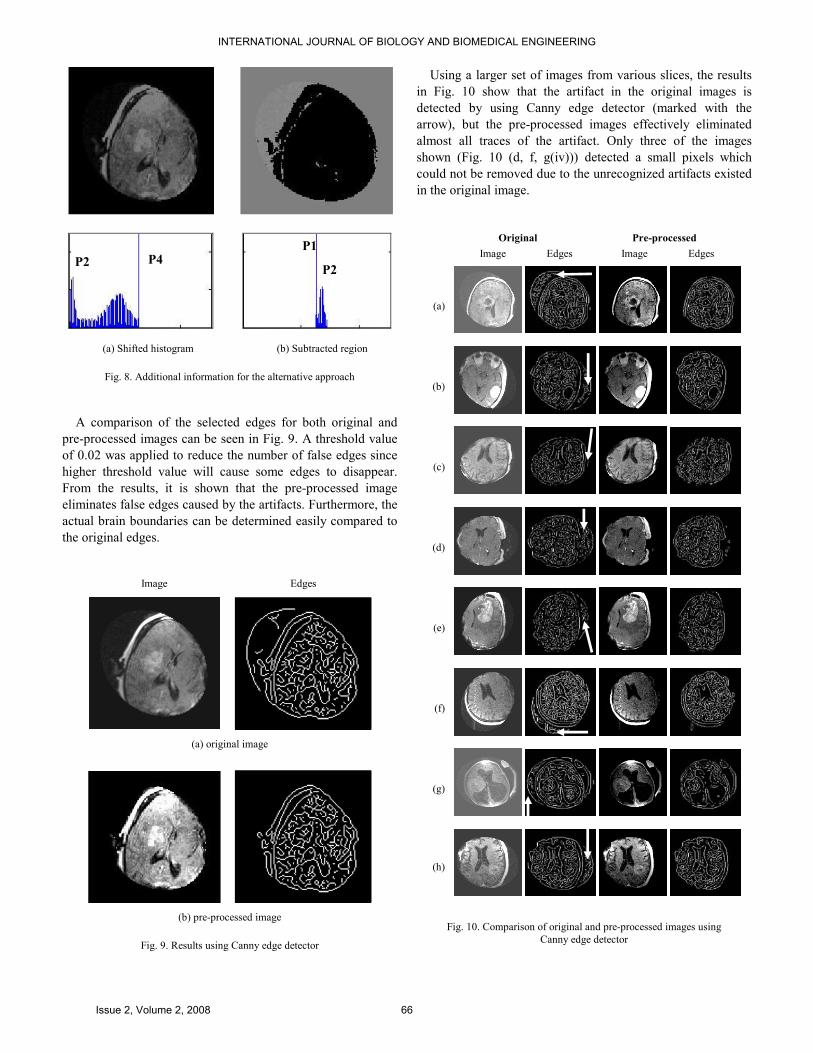
Using a larger set of images from various slices, the results

in Fig. 10 show that the artifact in the original images is

detected by using Canny edge detector (marked with the

arrow), but the pre-processed images effectively eliminated

almost all traces of the artifact. Only three of the images

shown (Fig. 10 (d, f, g(iv))) detected a small pixels which

could not be removed due to the unrecognized artifacts existed

in the original image.

Original Pre-processed

Image Edges Image Edges

(a)

(b)

(c)

(d)

(e)

(f)

(g)

(h)

Fig. 10. Comparison of original and pre-processed images using

Canny edge detector

P4 P2

P1

P2



D. Entropy

The effect of the proposed pre-processing technique can

also be quantified by measuring the image’s entropy, which is

the amount of its information content. Image data entropy can

be estimated from a gray level histogram. The entropy is

defined by (3).

Entropy i

i

i PLogP 2∑−= (3)

where Pi is the probability that the difference between two

adjacent pixels is equal to i, and Log2 is the base 2 logarithm.

According to [22], a relatively complex image has higher

entropy than a relatively simple image. As an example, an

image that is perfectly flat will have an entropy of zero while

high entropy images such as an image of heavily cratered areas

on the moon have a great deal of contrast from one pixel to the

next.

In Table 1 and 2, the entropy of the original and normalized

pre-processed images is shown for normal brain images (Fig.

6) and diseased brain images (Fig. 7), respectively. As stated

previously, the entropy is higher for complex images, as

compared to simple ones. In this case, the original image is

more complex image due to the texture caused by the noise.

Hence, the entropy should decrease as the image is

normalized.

TABLE 1: ENTROPY FOR NORMAL BRAIN

IMAGES

(FIG. 6)

ORIGINAL NORMALIZED

(a) 3.7564 3.3220

(b) 3.6214 3.6107

(c) 3.9211 3.4492

(d) 4.1783 4.1783

(e) 3.8138 3.8138

(f) 4.4469 3.5379

TABLE 2: ENTROPY FOR DISEASED BRAIN

IMAGES

(FIG. 7)

ORIGINAL NORMALIZED

(a) 4.4329 3.6600

(b) 4.2075 3.0363

(c) 4.4215 3.4455

(d) 4.2535 4.2535

(e) 4.3713 3.8561

(f) 3.7961 2.9920

(g) 4.1707 3.4132

(h) 4.5571 3.8577

(i) 4.2039 3.4218

(j) 4.3762 3.5560

(k) 4.4725 4.0331

(l) 4.1644 2.4366

From the results in Table 1 for normal brain images, it can

be seen that the entropy for most of the normalized images is

less than those of the original images. However, for Fig. 6(d)

and (e), there was no difference due to the minimum existence

of artifact in the original images.

By referring to Table 2 which consists of various brain

diseases, it is observed that the same results were achieved as

well. There is only one image (Fig. 7(d)) where there was no

obvious artifact in the original image.

All the results above prove the effectiveness of the proposed

scheme in clearing up the low-field brain MRI images. The

normalized pre-processed images are not only visually

improved, they are also more accurate for the purposes of

segmentation and other computer-aided tasks.

V. CONCLUSION

Low-field MRI is now being introduced in medical

institutions for real-time imaging during brain surgeries.

However, the low signal strength produces low-resolution

images and leads to difficulty in automated techniques.

This work proposes a dynamic thresholding and image

normalization technique for enhancement of low-field brain

MRI images. By controlled truncating and normalizing the

histogram, the scheme eliminates the unnecessary background

noise and artifacts in the image. The clarity of the ROI was

enhanced effectively while almost no loss of information or

image integrity was recorded in the actual brain areas of the

processed low-field MRI images.

It is shown in this paper that in the histogram of a typical

low-field MRI image, the first peak tends to be the image

background, with the second peak being the acquisition

artifact. The part of concern is the intensity around the third

peak, which consists of the main brain regions.

As qualitative visual human observation may be subjective,

quantitative measurement has also been taken into account to

evaluate the differences between the original and pre-

processed images. Out of entire database tested, minor

inaccuracy (1 for normal and 2 for diseased) have been

detected. Thus, the results show that more than 85% of the test

images performed as expected in eliminating all non-ROI

parts.

In future, further evaluation on special cases, such as the

existing of non-removable artifacts of the histogram will be

undertaken. The finalized image normalization technique

could be used directly for feature extraction and segmentation.

However, it is recommended that after pre-processing the

image, denoising filters should be applied to remove any

residue noise that may still present in the image, as proposed

in [23]. The efficiency, robustness and accuracy of the pre-

processing performance could be improved with further

detailed analysis.



ACKNOWLEDGMENT

The authors would like to thank the Department of

Neurosurgery, Maastricht University Hospital and the

Department of Biomedical Engineering, Eindhoven University

of Technology (TU/e), for providing the low-field MRI images

used in this study. This project was supported by the Ministry

of Science, Technology and Innovation (MOSTI), Malaysia

through the Science Fund grant.

REFERENCES

[1] F. Ségonne, A.M. Dale, E. Busa, M. Glessner, D. Salat, H.K. Hahn, B.

Fischl, “A hybrid approach to the skull stripping problem in MRI,”

NeuroImage, vol. 22, pp. 1060-1075, 2004.

[2] I.V. Gribkov, P.P Koltsov, N.V. Kotovich, A.A. Kravchenko, A.S.

Koutsaev, A.S. Osipov, A.V. Zakharov, “Testing of image segmentation

methods”, WSEAS Trans on Signal Processing, Vol. 7, 2008.

[3] K. Rehm, “Medical Image Segmentation,” Lecture Notes on Advance

Digital Imaging Science, University of Minnesota, 2002.

[4] J. Rexilius, H.K. Hahn, J. Klein, M.G. Lentschig, H.O. Peitgen,

“Multispectral brain tumor segmentation based on histogram model

adaptation,” Proceedings of SPIE Conference on Medical Image

Computing, vol. 4, pp. 65140V-1-65140V-10, 2007.

[5] U. Vovk, F. Pernu, B. Likar, “Simultaneous correlation of intensity

inhomogeneity in multichannel MR images,” 27th Annual Conf.

Engineering in Medicine and Biology, pp. 4290-4293, 2005.

[6] N.I. Weisenfeld, S.K. Warfield, “Normalization of joint image-intensity

statistics in MRI using the Kullback-Leibler divergence,” IEEE

Symposium on Biomedical Imaging : Nano to Macro, vol. 1, pp. 101-

104, 2004.

[7] A. Madabhushi, J.K. Udupa, “Interplay between intensity

standardization and inhomogeneity correction in MR image

processing,” IEEE Trans. on Medical Imaging, vol. 24, pp. 561-576,

2005.

[8] U. Vovk, F. Pernus, B. Likar, “A review of methods for correction of

intensity inhomogeneity in MRI,” IEEE Trans. on Medical Imaging,

vol. 26, pp. 405-421, 2007.

[9] Y.L. Liao, N.T. Chiu, C.M. Weng, Y.N. Sun, “Registration and

normalization techniques for assessing brain functional images,”

Biomedical Engineering Applications, Basis & Communications, 2003.

[10] J.G. Park, T. Jeong, C. Lee, “Automated brain segmentation algorithm

for 3D magnetic resonance brain images,” 2nd Intl. Workshop on Soft

Computing Applications (SOFA), pp. 57-61, 2007.

[11] Y. Zhengmao, M. Habib, Y. Yongmau, “Digital trimulus color image

enhancing and quantitative information measuring,” 6th WSEAS Intl.

Conf. on Information Security and Privacy, pp. 323-328, 2007.

[12] N.F. Ishak, M.J. Gangeh, and R. Logeswaran, “A preliminary study of

high-field MRI image enhancement techniques applied to low-field MR

brain images,” 4th Intl. Conf. on Biomedical Engineering (BIOMED),

vol. 21, pp. 482-486, 2008.

[13] M. Ballan, F. Gurgen, “Gradient based fingerprint verification using

principal components,” IEEE Advances in Intelligence Systems and

Computer Design (IMACS), pp. 191 – 196, 1999.

[14] A.S. Rosalina, S.K. Tan, A.R. Nuraini, “Live-cell image enhancement

using center weighted median filter,” 11th WSEAS Intl. Conf. on

Computers, pp. 382-385, 2007.

[15] H.A. Ali, B.M. Ne’ma, “Multi-purpose code generation using

fingerprint images”, 6th WSEAS Intl. Conf. on Information Security and

Privacy, pp. 141-145, 2007.

[16] N. Savage, “A weaker, cheaper MRI,” IEEE Spectrum, vol. 45, no. 1,

pp. 21, January 2008.

[17] P. Hastreiter, C.R. Salama, G. Soza, M. Baeur, et. al, “Strategies for

brain shift evaluation,” Medical Image Analysis, vol. 8, pp. 447-464,

2004.

[18] T. Magee, M. Shapiro, and D. Williams, “Comparison of high-field-

strength versus low-field-strength MRI of the shoulder,” American

Journal of Roentgenology, pp. 1211-1215, 2003.

[19] M.B. Ahmad, and T.S. Choi, “Local threshold and Boolean function

based edge detection,” IEEE Trans. On Consumer Electronics, vol. 45,

pp. 332-333, 1999.

[20] C.S. Yung, S.H. Ki, M.N. Seung, and W.P. Jong, “Threshold estimation

for region segmentation of MR image of brain having the partial volume

artifact,” 5th Intl. Conf. on Signal Processing Proceedings (ICSP), vol.

2, pp. 1000-1009, 2000.

[21] J.F. Canny, “A computational approach to edge detection.” IEEE Trans.

On Pattern Analysis and Machine Intelligence (PAMI), vol. 8, pp. 679-

698, 1986.

[22] Y. Zhengmao, M. Habib, Y. Yongmau, “Image contrast enhancement

and quantitative measuring of information flow,” 6th WSEAS Intl. Conf.

on Information Security and Privacy, pp. 172-177, 2007.

[23] N.F. Ishak, M.J. Gangeh, and R. Logeswaran, “Comparison of denoising

techniques applied on low-field MR brain images,” 5th Intl. Conf. on

Computer Graphics, Imaging and Visualization (CGIV), pp. 345–349,

2008.

Nur Faiza Ishak was born in Kuala Lumpur, Malaysia on the February 08th,

1984. She received the B. Eng. (Hons) degree in Electronics (majoring in

Telecommunications) from the Faculty of Engineering and Technology,

Multimedia University, Melaka, Malaysia in 2007.

She is currently a Research Officer at the Faculty of Engineering,

Multimedia University, Cyberjaya, Selangor, Malaysia. Her research areas are

in image processing, low-field MRI and brain segmentation.

Rajasvaran Logeswaran received his B. Eng. (Hons) Computing degree

from the University of London (Imperial College of Science, Technology and

Medicine), United Kingdom in 1997, M.Eng.Sc. and Ph.D. degrees from

Multimedia University, Cyberjaya in 2000 and 2006, respectively.

He was an Assistant Professor at The Global School of Media, Soongsil

University, South Korea in 2008. He is currently a Senior Lecturer at the

Faculty of Engineering, Multimedia University, Cyberjaya, Malaysia. His

research interests comprises of neural network, data compression, medical

image processing and web technology.

Tan Wooi Haw received his M. Sc. (Electronics) from Queen’s University of

Belfast in 1998. His research interest is in image processing and analysis, as

well as swarm intelligence. He is a Lecturer at the Faculty of Engineering,

Multimedia University, Cyberjaya, Malaysia.



Artifact and noise stripping on low-field brain MRI · Abstract—Low-field Magnetic Resonance...

Documents

Transcript of Artifact and noise stripping on low-field brain MRI · Abstract—Low-field Magnetic Resonance...