Articulated Hub Model for 3D Aeromechanical Simulation of ...
130
Articulated Hub Model for 3D Aeromechanical Simulation of Helicopter Rotors by Michael G. Martin, B. Eng. Carleton University A thesis submitted to the Faculty of Graduate Studies and Research in partial fulfillment of the requirements for the degree of Master of Applied Science Ottawa-Carleton Institute for Mechanical and Aerospace Engineering Department of Mechanical and Aerospace Engineering Carleton University Ottawa, Ontario September 2011 © Copyright 2011 - Michael G. Martin l
Transcript of Articulated Hub Model for 3D Aeromechanical Simulation of ...
Articulated Hub Model for 3D Aeromechanical Simulation of Helicopter Rotors
by
Michael G. Martin, B. Eng.
Carleton University
A thesis submitted to
the Faculty of Graduate Studies and Research
in partial fulfillment of
the requirements for the degree of
Master of Applied Science
Ottawa-Carleton Institute for
Mechanical and Aerospace Engineering
Department of
Mechanical and Aerospace Engineering
Carleton University
Ottawa, Ontario
September 2011
© Copyright
2011 - Michael G. Martin
l
1*1 Library and Archives Canada
Published Heritage Branch
395 Wellington Street OttawaONK1A0N4 Canada
Bibliotheque et Archives Canada
Direction du Patrimoine de I'edition
395, rue Wellington OttawaONK1A0N4 Canada
Your file Votre reference ISBN: 978-0-494-83038-3 Our file Notre r6f6rence ISBN: 978-0-494-83038-3
NOTICE:
The author has granted a nonexclusive license allowing Library and Archives Canada to reproduce, publish, archive, preserve, conserve, communicate to the public by telecommunication or on the Internet, loan, distribute and sell theses worldwide, for commercial or noncommercial purposes, in microform, paper, electronic and/or any other formats.
AVIS:
L'auteur a accorde une licence non exclusive permettant a la Bibliotheque et Archives Canada de reproduire, publier, archiver, sauvegarder, conserver, transmettre au public par telecommunication ou par I'lnternet, preter, distribuer et vendre des theses partout dans le monde, a des fins commerciales ou autres, sur support microforme, papier, electronique et/ou autres formats.
The author retains copyright ownership and moral rights in this thesis. Neither the thesis nor substantial extracts from it may be printed or otherwise reproduced without the author's permission.
L'auteur conserve la propriete du droit d'auteur et des droits moraux qui protege cette these. Ni la these ni des extraits substantiels de celle-ci ne doivent etre imprimes ou autrement reproduits sans son autorisation.
In compliance with the Canadian Privacy Act some supporting forms may have been removed from this thesis.
Conformement a la loi canadienne sur la protection de la vie privee, quelques formulaires secondaires ont ete enleves de cette these.
While these forms may be included in the document page count, their removal does not represent any loss of content from the thesis.
Bien que ces formulaires aient inclus dans la pagination, il n'y aura aucun contenu manquant.
1+1
Canada
The undersigned recommend to
the Faculty of Graduate Studies and Research
acceptance of the thesis
Articulated Hub Model for 3D Aeromechanical Simulation of Helicopter Rotors
submitted by
Michael G. Martin, B. Eng.
in partial fulfillment of the requirements for
the degree of
Master of Applied Science
F. Nitzsche, Thesis Supervisor
D. Feszty, Thesis Supervisor
M. I. Yaras, Chair, Department of Mechanical and Aerospace Engineering
Carleton University
September 2011
u
Abstract
The SMARTROTOR code is a 3D aeroelastic computational tool for the simulation of
helicopter rotor aeromechanics. This code has been created through collaborated work of
interfacing aerodynamic, structural, and dynamic models. The aerodynamic model was adapted
from the GENUVP discrete vortex method which was originally developed for studying wind
turbine blades and its surrounding wake environment. Therefore, the current version of the
SMARTROTOR code allows modeling of a hingeless blades based on the Hodges non-linear
deformation equations. However, since helicopter blades are hinged, i.e. articulated at their root,
the code only allowed modeling of hingeless rotors in the past. The objective of the work
presented herein was to add hinges to the dynamic model of SMARTROTOR, while assuming
rigid blades. The rigid blade hinged model is based on the equations of motion presented in J.G.
Leishman's Principles of Helicopter Aerodynamics. The new model is validated by comparing
simulations to F.D. Harris' experiment on a scaled articulated rotor at various advance ratios,
shaft tilts and collective pitch settings. Comparison of blade angle, amplitudes and paths for the
flapping and lead-lag motions indicate that the articulated rotor hub model captures key blade
dynamics accurately.
111

Acknowledgements
I would like to thank my supervisors Professor Fred Nitzsche and Professor Daniel
Feszty for granting me the opportunity to join Carleton Rotorcraft Research Group and allow me
to make a contribution to the SMARTROTOR program. I would like to acknowledge the help of
Gregory Oxley, Sean McTavish, and Derek Gransden for introducing me to the basic workings
of the SMARTROTOR program. I would like to acknowledge the assistance of Neil McFayden
and Bruce Johnston for allowing me access to the Department's Linux servers and their
associated services in keeping me connected when I worked off site.
I would like to thank the Canada-EU Student Exchange Program in Aerospace
Engineering and Prof. Eric Gillies at the University of Glasgow for their support in permitting
me to study this program in Glasgow, Scotland.
I would like thank my parents David and Ann Martin for encouragement and help at
times of challenge, to value this education and apply it to one's current and future vocational
activities.
I would like to thank Voyageur Airways Ltd. in North Bay, Ontario, my current employer
for allowing me to enter the ever interesting and exciting aerospace industry while completing
my graduate studies. In particular I would like to thank my supervisors Georges Dubytz, Jeff
MacFarlane, Jeff Cooke, and company President, Max Shapiro for their continued support and
patience as I worked on this project. On this subject I would like to thank again Fred and Daniel,
the Department of Mechanical and Aerospace Engineering, and the Graduate Studies Department
for permitting me to begin my Engineering career while working on these studies part time and
several hundred kilometers away from the University.
iv
List of Symbols
a
ai
Aic
bi
SA
b
B
Bic
C\(
cD
cL
CL«
CM
CT
D
r-Ba f-Bb
DELTAX
DISP
Disp_ Disp. Disp_
.ID
.2D
.3D
Global frame, Chapter 2
Lateral flapping angle, Chapter 4
Lateral cyclic, Chapter 4
Harris flap coefficient, Chapter 4
Change in the spatial domain, Chapter 2
Local undeformed frame, Chapter 2
Local deformed frame, Chapter 2
Longitudinal cyclic, Chapter 4
Transformational matricies, Chapter 2
Drag coefficient, Chapter 2
Lift coefficient, Chapter 2
Lift slope coefficient, Chapter 4
Pitching moment coefficient, Chapter 2
Thrust coefficient, Chapter 4
Drag, Chapter 1
Node displacements used in TWIST 123 subroutine, Chapter 3
Spanwise aero node displacements used in MAP_DEFORM subroutine, Chapter 3
Spanwise structural node displacements used in TRAN subroutine, Chapter 3
e Hinge offset faction of blade radius, Chapter 3
F Internal force vector, Chapter 2
F Force segment, Chapter 3
H
i
J
K
L
L
m
M
n
N
P
R
RAXIS
Rot
t
Trans
Twist_ Twist_ Twist_
.ID 2D 3D
u
U
Angular momentum vector, Chapter 2
Spanwise index, Chapter 3
Moment of inertia (flapwise and lagwise), Chapter 3
Chordwise index, Chapter 3
Potential energy density, Chapter 2
Lift, Chapter 1
Blade length, Chapter 4
Mass distribution, Chapter 3, 4
Internal moment vector, Chapter 2
Spanwise node index, Chapter 3
Max spanwise node index, Chapter 2
Linear momentum vector, Chapter 2
Blade radial measure from center of rotation, Chapter 1
Blade radius, Chapter 1
Aero chordwise node displacement used in TWIST 123 subroutine, Chapter 3
Denavit-Hartenberg rotational transform matrix, Chapter 3
Time, Chapter 2
Denavit-Hartenberg displacement transform matrix, Chapter 3
Spanwise structural node orientations used in TRAN subroutine, Chapter 3
Displacement measure, Chapter 2
Flowfield velocity as a function of position and time, Chapter 2
Strain energy density, Chapter 2
vi
V Velocity, Chapter 1
V, Incident velocity, Chapter 1
VR Resultant velocity, Chapter 1
VTip Tip velocity, Chapter 1
Voo Incoming velocity, Chapter 1
8W Change in the virtual work, Chapter 2
x Chordwise displacement (local frame of reference), Chapter 3
x Position vector, Chapter 2
X Vector that described the structural state of the rotor blade, Chapter 2
XFTNAL Final aero node positions in TWIST 123 subroutine, Chapter 3
XINIT Undeformed aero node positions in TWIST 123 subroutine, Chapter 3
XROTATE Aero node positions in TWIST 123 subroutine, Chapter 3
y Spanwise displacement (local frame of reference), Chapter 3
Ya, Yb, Ya Beam node vectors, Chapter 2
z Vertical displacement (local frame of reference), Chapter 3
a Angle of attack, Chapter 1
(XTPP Tip path plane angle, Chapter 2
/? Flap angle, Chapters 1
Po Mean flap angle, Chapter 2
C Lag angle, Chapter 1
6 Angular orientation measure, Chapter 2
6 Pitch angle, Chapter 3
60 Root pitch angle, Chapter 4
vii
075
Otw
X
V
p
Vb,V£
a
¥
Q
n C) ( • )
( " )
Pitch angle at the 75% radius station, Chapter 4
Blade twist per unit length of blade, Chapter 4
Inflow ratio, Chapter 4
Advance ratio, Chapter 4
Air density, Chapter 4
Frequency (flapping and lagging), Chapter 3
Solidity, Chapter 4
Azimuth angle, Chapter 4
Rotor rotational velocity, Chapter 1
Vector, Chapter 2
Beam boundary value, Chapter 2
Velocity, Chapter 3
Acceleration, Chapter 3
Vlll
Contents Abstract iii
Acknowledgements iv
List of Symbols v
List of Figures xi
List of Tables xiii
Chapter 1 Introduction 1
1.1 Background 1
1.2 The Need for Blade Flapping 2
1.3 Aerodynamics of the Blade Flapping 6
1.4 The Need for Lead-Lag Hinges 7
1.5 The Need for Feathering Hinge 9
1.6 Rotor Hub Types 9
1.7 Rotor Control Via Swashplate 11
1.8 Blade Elastic Deformation 12
1.9 Computational Aeroelastic Codes 13
1.10 Thesis Objectives 15
1.11 Thesis Structure 15
Chapter 2 SMARTROTOR Background 17
2.1 GENUVP Overview 17
2.2 STRUCTDEFORM Overview 21
Chapter 3 Rotating Rigid Blade Model 26
3.1 Rotating Rigid Blade Overview 26
3.2 Coupling Rigid Motion with Aerodynamics 31
3.3 Interpolation from Aerodynamic Model to Rigid Blade Model 34
3.4 Interpolation from Rigid Blade Model to Aerodynamic Model 34
Chapter 4 CH-47C Rotor Blade Flapping Motion Analysis 43
4.1 Harris Articulated Blade Flapping Motion Overview 44
4.2 CH47C Airfoil 45
4.3 Harris Simulation: Influence of Collective Pitch 49
4.4 Harris Simulation: Influence of Advance Ratio 62
4.5 Harris Simulation: Influence of Shaft Tilt 67
Chapter 5 Summary, Conclusions and Recommendations 72
5.1 Summary 72
IX
5.2 Conclusions 73
5.3 Recommendations 73
References 75
Appendix A SMARTROTOR User's Guide and Input Files 78
A.1 SMARTROTOR Operators Guide 78
A.2 atfile 80
A.3 fare 80
A.4 CH47CHL.dat 81
A.5 CH47C.geo 84
A.6 CH47C.bld 87
A.7 23573.cld 88
A.6 inputc.dat 91
Appendix B SMARTROTOR Amended Source Code 94
B.l COMBINED_C.f 94
B.2 gnvp-3.coupled.f 96
B.3 blade_deform.f 99
B.4 bladeartie.f 105
B.5 odeblade.f 107
B.6 couple.f 108
B.7 chinge.f. 116
x
List of Figures
Figure 1.1 - Comparison of fixed-wing and rotary-wing lift and incident velocity distributions...3 Figure 1.2 - Comparison of incident velocity distribution on rotor blades between (a) hovering flight and (b) forward flight [1] 4 Figure 1.3 - Imbalance of rotor disk in forward flight 5 Figure 1.4 - Blade flapping on Juan de la Cierva's C.8 Autogiro [3] 6 Figure 1.5 - Reduction or increase in lift due to blade flapping 7 Figure 1.6 - Figure skating spinning speed as a function of arm displacement 8 Figure 1.7 - "Lead-lag" hinge allows for in-plane rotation 8 Figure 1.8-Rotor types [4] 10 Figure 1.9 - Swashplate on a UH-1M Iroquois (Bell Model 204) [4] 11
Figure 2.1 - 3 D Visualization of the wake model 19 Figure 2.2 - Top-level block diagram of GENUVP 20 Figure 2.3 -Schematic of lift and drag calculations 21 Figure 2.4 - Illustrated comparison of hingeless and hinged rotors [15] 22 Figure 2.5 - A schematic Diagram of the coordinate frames used by the structural component in STRUCTDEFORM [8] 23
Figure 3.1 -Flapping lead-lag and feathering motion of a rotor blade [1] 27 Figure 3.2 -Equilibrium of blade forces about the flapping hinge [1] 28 Figure 3.3 -Equilibrium of blade forces about the lead-lagging hinge [1] 28 Figure 3.4 - Blade discretized lift and drag profiles 30 Figure 3.5 - Original SMARTROTOR main subroutine flow chart 32 Figure 3.6 - Modified SMARTROTOR main subroutine flow chart 33 Figure 3.7 - Rigid blade model coordinate system 35 Figure 3.8 - Temporary aerodynamic node linear grid 38 Figure 3.9 - Displacing aerodynamic nodes from undeformed position 41 Figure 3.10-Aerodynamic blade model coordinate system. 42
Figure 4.1 - Vertol division helicopter model [9] 43 Figure 4.2 - V23010-1.58 airfoil lift curves as shown in [21] 46 Figure 4.3 - V23010-1.58 airfoil drag curves as shown in [21] 46 Figure 4.4 - V23010-1.58 airfoil pitching moment curves as shown in [21] 47 Figure 4.5 - V23010-1.58 airfoil lift curves as set up in SMARTROTOR 48 Figure 4.6 - V23010-1.58 airfoil drag curves as set up in SMARTROTOR 48 Figure 4.7 - V23010-1.58 airfoil pitching moment curves as set up in SMARTROTOR 49 Figure 4.8 - Flap Angle Vs. Azimuth Position - Collective Pitch d75 = 8.83° 50 Figure 4.9 - Helicopter azimuth reference positions 51 Figure 4.10 - 3D Visualization of rotor path (4 blades, pitch 13.05°, last 36° sweep) 53 Figure 4.11 -Vertical tip path of blade 1 (pitch d15 = 13.05°) 54 Figure 4.12 - Flap and lead-lag angles of blade 1 (pitch 675 = 13.05°) 54 Figure 4.13 -The blade lagging frequency varies with the hinge offset [1] 55 Figure 4.14 -Blade lift histories (pitch 015 = 13.05°) 56 Figure 4.15 - Flap angle comparison between twisted and untwisted blades 57
XI
Figure 4.16 - Influence of Collective Pitch - pitch vs. Cj/a. 58 Figure 4.17 - Influence of Collective Pitch - pitch vs. flap amplitude 58 Figure 4.18 -Comparison of Harris & SMARTROTOR flap angles 59 Figure 4.19 - Out-of-phase azimuth lag between simulation & Harris test 60 Figure 4.20 - Influence of Collective Pitch - Harris experiment flap path 61 Figure 4.21 - Influence of Collective Pitch - SMARTROTOR flap path 62 Figure 4.22 - Influence of Advance Ratio - comparison of thrust coefficients 64 Figure 4.23 -Influence of Advance Ratio - comparison of flap amplitude 65 Figure 4.24 - Influence of Advance Ratio - Harris flap angles 66 Figure 4.25 - Influence of Advance Ratio - SMARTROTOR flap angles 67 Figure 4.26 - Influence of Shaft Tilt - comparison of thrust coefficients 69 Figure 4.27 - Influence of Shaft Tilt - comparison of flap amplitude 69 Figure 4.28 - Influence of Shaft Tilt - Harris flap angles 70 Figure 4.29 - Influence of Shaft Tilt - SMARTROTOR flap angles 70
xn
List of Tables
Table 4.1-CH47C scaled rotor geometry 44 Table 4.2 - Harris collective pitch experiment results 49 Table 4.3 - Harris simulation parameters 52 Table 4.4 - SMARTROTOR results for CH47C rotor blade model 57 Table 4.5 - Influence of CoUective Pitch - SMARTROTOR results flap angle coefficients 61 Table 4.6 - Harris' Influence of Advance Ratio experiment results 63 Table 4.7 -Harris' Influence of Advance Ratio flap angle coefficients 63 Table 4.8 - SMARTROTOR results for CH47C rotor blade model 64 Table 4.9 - Influence of Advance Ratio - SMARTROTOR results flap angle coefficient 66 Table 4.10 - Harris' Influence of Shaft Tilt experiment results 68 Table 4.11 - SMARTROTOR results for CH47C rotor blade model 68 Table 4.12 - Influence of Shaft Tilt - SMARTROTOR results flap angle coefficient 70
xin
Chapter 1 - Introduction
Chapter 1 Introduction
1.1 Background
The helicopter is a transport vehicle, which has become indispensible in the modern
world. While the airplane contributes greatly to international commerce, transport, and military
applications, the helicopter has special niches. The ability of vertical take-off and slow flight
maneuverability has found its place in such roles as transportation, geological surveying, forest
fire fighting, search and rescue operations, and personal recreation, among others. The need for
continuing technological advancement in this field presents opportunities to study and develop
methods to improve helicopter research and designs.
One particular area of interest of the helicopter community is the study of rotor wing
aeroelasticity. The challenge in modeling elastic rotating wings is that one must take into account
the blade's rotational dynamics, elastic dynamics, and aerodynamics. There is an interest to
model this complicated system of motion, so that various research activities related to studying
helicopter vibration, rotor blade design, and helicopter noise can be accomplished.
The Rotorcraft Research Group at Carleton University, in collaboration with the National
Technical University of Athens (Greece) and the Massachusetts Institute of Technology
(U.S.A.), has developed a rotorcraft aeroelastic code called SMARTROTOR. This can simulate
the motions and deformations of elastic helicopter and wind turbine blades. However, the present
version of SMARTROTOR allows the modeling of hingeless rotors only. This is because the
origins of SMARTROTOR began as a wind turbine rigid blade simulation tool, used to predict
the aerodynamic performance of wind turbine blades, including the downstream wake
1
Chapter 1 - Introduction
environment. However, while wind turbine blades are rigidly attached at their root (i.e.
cantilevered), helicopter blades must be articulated (i.e. hinged) at their root to allow two degrees
of freedom during rotation to provide a balance of aerodynamic forces on the rotor.
Unfortunately, the present version of SMARTROTOR does not allow to model articulated rotors,
hence the main objective of this thesis is to address this issue.
The next sections will describe in detail the need for blade articulation for helicopters, the
state-of-the-art in employing such models, and the need for this model in the SMARTROTOR
code.
1.2 The Need for Blade Flapping
Why is the hinge configuration important to rotorcraft systems? In short, hinges allow the
helicopter's rotor blades to resolve an imbalance created by the lifting forces generated on the
blades in forward flight. A general explanation of the aerodynamics of rotor blade hinges is as
follows.
Helicopters generate thrust (or commonly referred to as lift) by rotating the lifting
surfaces, known as blades. Helicopter blades are essentially rotating wings, which create lift by
generating pressure difference between the upper and lower surfaces. Unlike fixed wings on
aircraft, rotory wings generate a linear lift distribution across the blade as illustrated in Figure
1.1.
2
Chapter 1 - Introduction
L'nifrom Lift-,
Incident Velocity. v = Vr > : ~
(Fixed-Wing)
Linear Lift
Tip Velocity K,.= QR '
Incident V V. = Qr
Velocity, / " " * * > / ' s / R
/ - y
(Rotary-Wing)
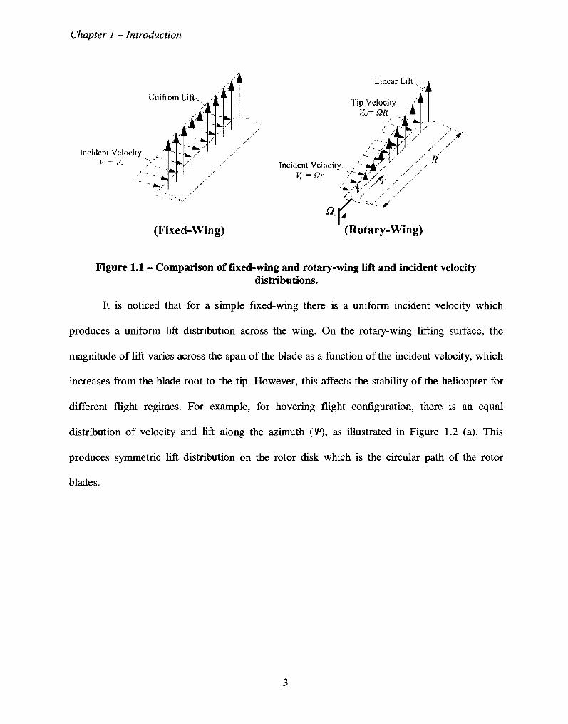
Figure 1.1 - Comparison of fixed-wing and rotary-wing lift and incident velocity
distributions.
It is noticed that for a simple fixed-wing there is a uniform incident velocity which
produces a uniform lift distribution across the wing. On the rotary-wing lifting surface, the
magnitude of lift varies across the span of the blade as a function of the incident velocity, which
increases from the blade root to the tip. However, this affects the stability of the helicopter for
different flight regimes. For example, for hovering flight configuration, there is an equal
distribution of velocity and lift along the azimuth (f), as illustrated in Figure 1.2 (a). This
produces symmetric lift distribution on the rotor disk which is the circular path of the rotor
blades.
3
Chapter 1 - Introduction
V,= 0.3OR
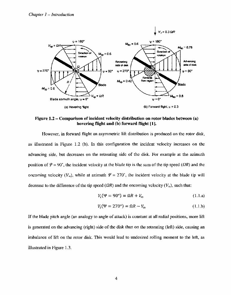
Figure 1.2 - Comparison of incident velocity distribution on rotor blades between (a) hovering flight and (b) forward flight [1].
However, in forward flight an asymmetric lift distribution is produced on the rotor disk,
as illustrated in Figure 1.2 (b). In this configuration the incident velocity increases on the
advancing side, but decreases on the retreating side of the disk. For example at the azimuth
position of !?= 90°, the incident velocity at the blade tip is the sum of the tip speed (QR) and the
oncoming velocity (Voo), while at azimuth W = 270°, the incident velocity at the blade tip will
decrease to the difference of the tip speed (QR) and the oncoming velocity (Vx), such that:
ViQV = 90°) = SIR + Vm (l.l.a)
VtQ¥ = 270o) = OR-Vm (l.l.b)
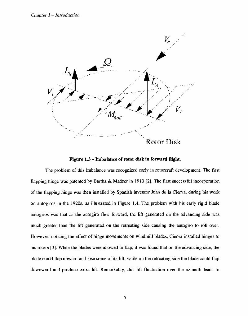
If the blade pitch angle (an analogy to angle of attack) is constant at all radial positions, more lift
is generated on the advancing (right) side of the disk than on the retreating (left) side, causing an
imbalance of lift on the rotor disk. This would lead to undesired rolling moment to the left, as
illustrated in Figure 1.3.
4
Chapter 1 - Introduction
K /
L A v, /V
Q
^i 1/ Roll
.4
y y <
If'/ ^ ,
s / • • — .
Rotor Disk
Figure 1.3 - Imbalance of rotor disk in forward flight.
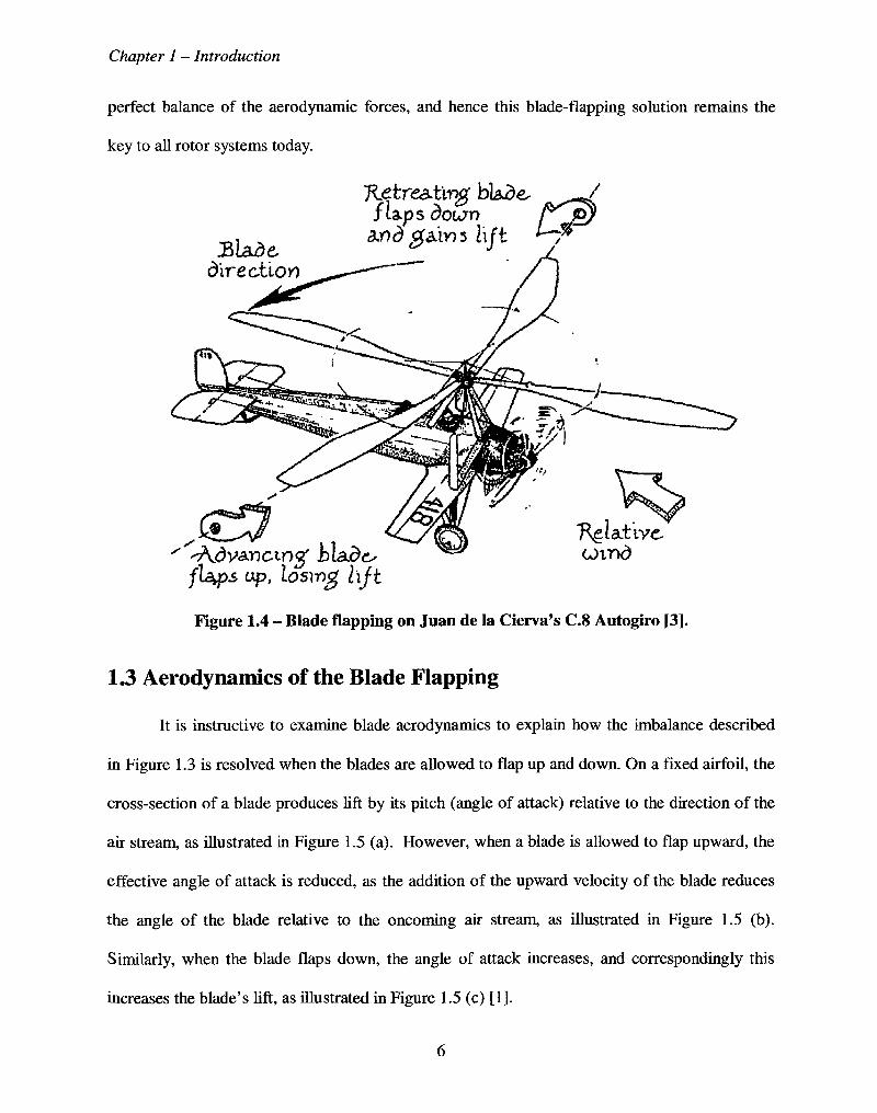
The problem of this imbalance was recognized early in rotorcraft development. The first
flapping hinge was patented by Bartha & Madzer in 1913 [2]. The first successful incorporation
of the flapping hinge was then installed by Spanish inventor Juan de la Cierva, during his work
on autogiros in the 1920s, as illustrated in Figure 1.4. The problem with his early rigid blade
autogiros was that as the autogiro flew forward, the lift generated on the advancing side was
much greater than the lift generated on the retreating side causing the autogiro to roll over.
However, noticing the effect of hinge movements on windmill blades, Cierva installed hinges to
his rotors [3]. When the blades were allowed to flap, it was found that on the advancing side, the
blade could flap upward and lose some of its lift, while on the retreating side the blade could flap
downward and produce extra lift. Remarkably, this lift fluctuation over the azimuth leads to
5
Chapter 1 - Introduction
perfect balance of the aerodynamic forces, and hence this blade-flapping solution remains the
key to all rotor systems today.
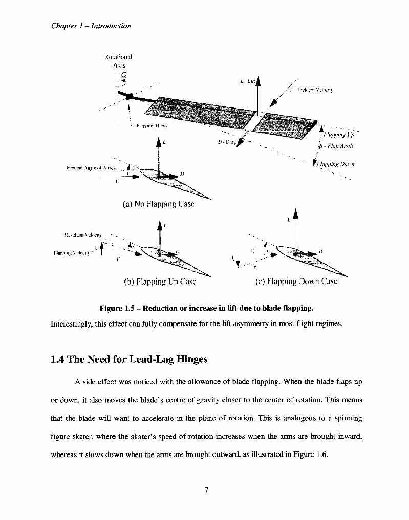
1.3 Aerodynamics of the Blade Flapping
It is instructive to examine blade aerodynamics to explain how the imbalance described
in Figure 1.3 is resolved when the blades are allowed to flap up and down. On a fixed airfoil, the
cross-section of a blade produces lift by its pitch (angle of attack) relative to the direction of the
air stream, as illustrated in Figure 1.5 (a). However, when a blade is allowed to flap upward, the
effective angle of attack is reduced, as the addition of the upward velocity of the blade reduces
the angle of the blade relative to the oncoming air stream, as illustrated in Figure 1.5 (b).
Similarly, when the blade flaps down, the angle of attack increases, and correspondingly this
increases the blade's lift, as illustrated in Figure 1.5 (c) [1].
6
Chapter 1 - Introduction
Rotational Axis
Incident Anjj.ciil Muck ...-4 a
(a) No Flapping Case
KoulLmt \ clt'ciU
i: i fanp m> \ cl(!cit\"' r-'̂
/I Inticcit V'.')IKI'\
(b) Flapping Up Case
-*-rs*«-P?
/• lapping (•/)
</} • Flap Angle
f Napping Down
4
•1 ..--"•'
(c) Flapping Down Case
Figure 1.5 - Reduction or increase in lift due to blade flapping.
Interestingly, this effect can fully compensate for the lift asymmetry in most flight regimes.
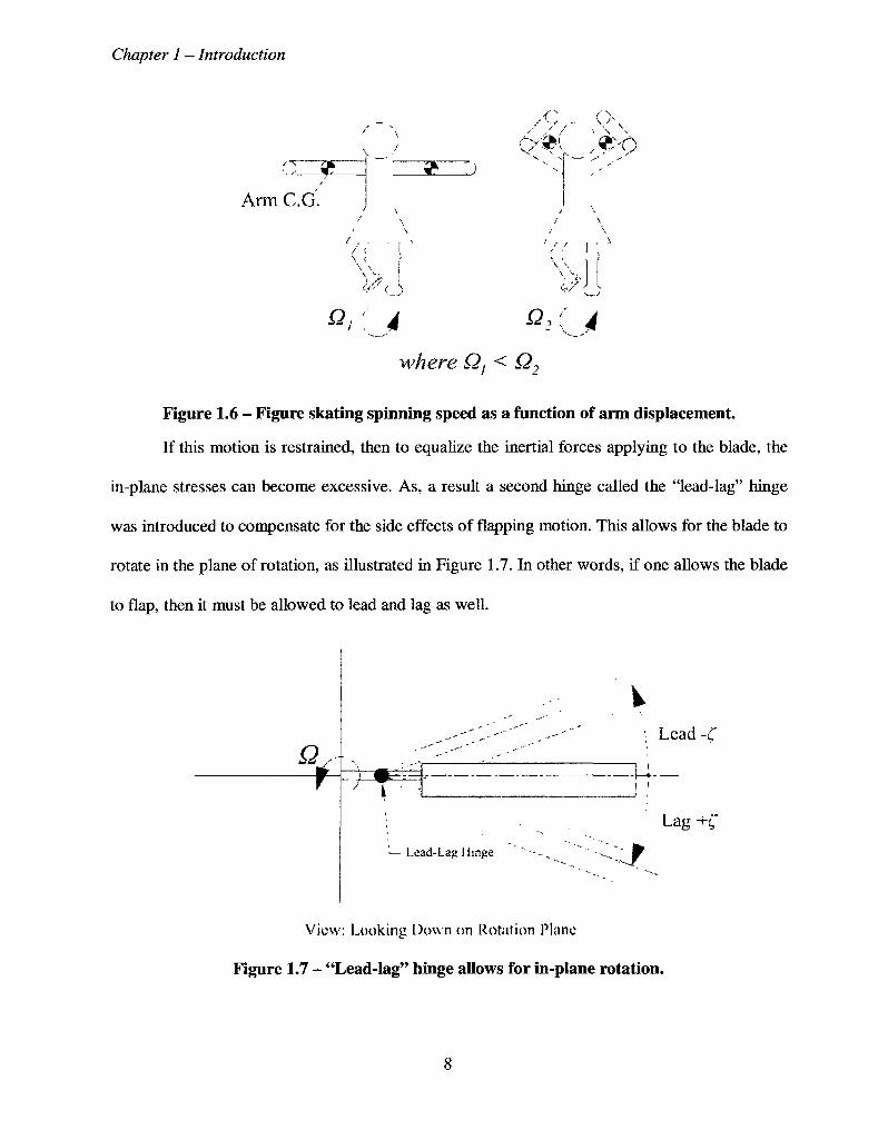
1.4 The Need for Lead-Lag Hinges
A side effect was noticed with the allowance of blade flapping. When the blade flaps up
or down, it also moves the blade's centre of gravity closer to the center of rotation. This means
that the blade will want to accelerate in the plane of rotation. This is analogous to a spinning
figure skater, where the skater's speed of rotation increases when the arms are brought inward,
whereas it slows down when the arms are brought outward, as illustrated in Figure 1.6.
7
Chapter 1 — Introduction
Arm C.G.
)?rl <•/' (
v ^ \ \ V i-
where Qj < Q2
Figure 1.6 - Figure skating spinning speed as a function of arm displacement.
If this motion is restrained, then to equalize the inertial forces applying to the blade, the
in-plane stresses can become excessive. As, a result a second hinge called the "lead-lag" hinge
was introduced to compensate for the side effects of flapping motion. This allows for the blade to
rotate in the plane of rotation, as illustrated in Figure 1.7. In other words, if one allows the blade
to flap, then it must be allowed to lead and lag as well.
Q 1-
•— Lead-Lag Hinge
Lead-C
Lag +C
View; Looking Down on Rotation Plane
Figure 1.7 - "Lead-lag" hinge allows for in-plane rotation.
8
Chapter 1 - Introduction
1.5 The Need for Feathering Hinge
There is a third hinge that allows the pilot to change the blade's pitch angle. It is called
the feathering hinge (see Figure 1.8 (b)). This controls the amount of thrust generated by the
rotor by controlling the pitch angle (i.e. angle of attack) of the blade. Unlike aircraft propellers
which are mostly controlled by adjusting the speed (RPM) of the blade (and yes, some propellers
do have pitch control which is similar to the helicopter's feathering hinge control), on helicopters
the RPM is fixed. Helicopters are designed to run at a constant RPM so that vibration resonance
with other parts of the hub and fuselage can be avoided. Therefore, to control the thrust, only the
blade's pitch angle is changed, and not the RPM.
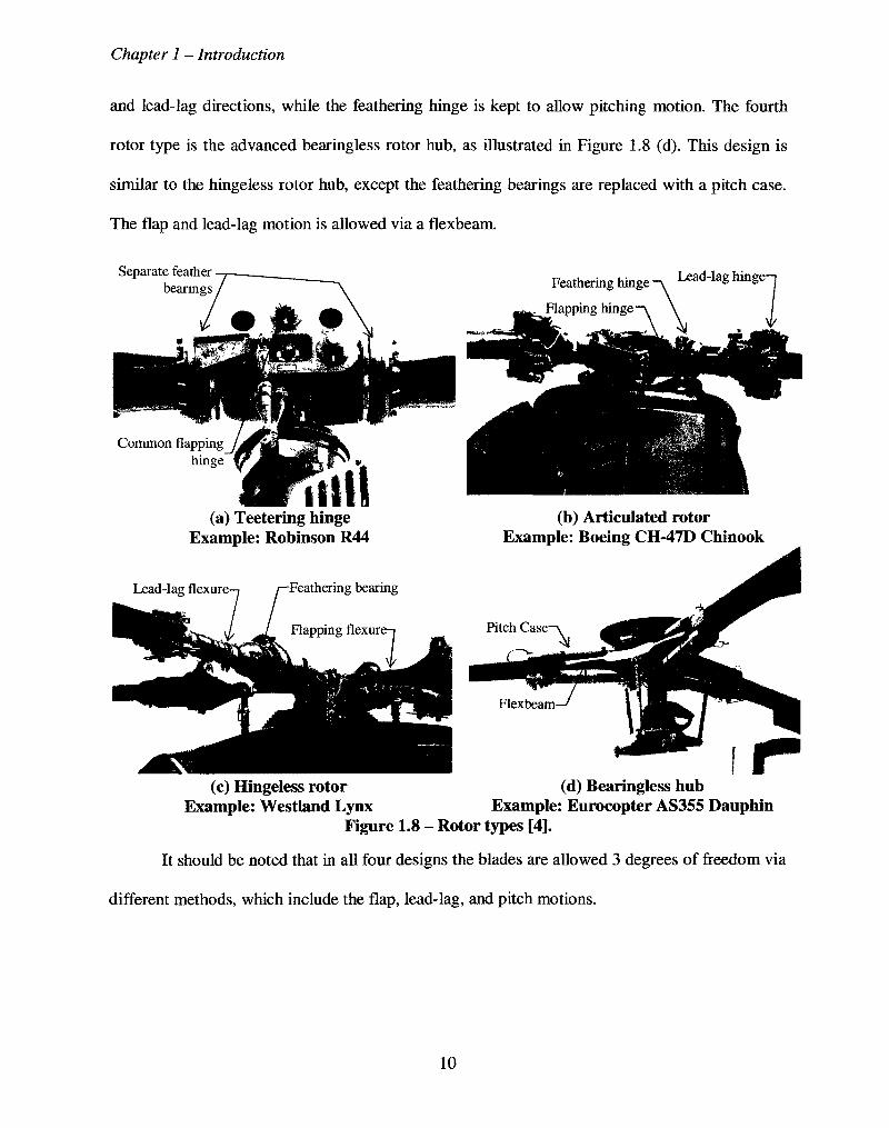
1.6 Rotor Hub Types
There are four fundamental types of helicopter rotor hubs in use: the teetering rotor hub,
the articulated rotor hub, the hingeless rotor hub, and the bearingless rotor hub. The teetering
rotor hub is the simplest, and consists of a single structure that is hinged at the rotational axis as
illustrated in Figure 1.8 (a). There are no independent flap hinges, and as such when the blade
flaps up, the other blade correspondingly flaps down like a seesaw. To allow for this motion each
blade has its own lead-lag hinge. The second rotor type is the articulated rotor hub, as illustrated
in Figure 1.8 (b). The articulated rotor hub consists of flapping and lead-lag hinges which are
free to rotate, while the feathering hinge is controlled by the collective and cyclic pitch input by
the pilot. This design is discussed in more detail in later chapters, and a module was created and
added to the SMARTROTOR program to simulate flight regimes with this rotor hub model. The
third rotor type is the hingeless rotor hub, as illustrated in Figure 1.8 (c), where the hinges of the
articulated design are replaced with flexures. The flexures allow for the blade to rotate in the flap
9
Chapter 1 - Introduction
and lead-lag directions, while the feathering hinge is kept to allow pitching motion. The fourth
rotor type is the advanced bearingless rotor hub, as illustrated in Figure 1.8 (d). This design is
similar to the hingeless rotor hub, except the feathering bearings are replaced with a pitch case.
The flap and lead-lag motion is allowed via a flexbeam.
Separate feather bearings Feathering hinge ~x 1**M»S h™&-
Flapping hinge
(a) Teetering hinge Example: Robinson R44
Lead-lag flexure
(b) Articulated rotor Example: Boeing CH-47D Chinook
(c) Hingeless rotor (d) Bearingless hub Example: Westland Lynx Example: Eurocopter AS355 Dauphin
Figure 1.8 - Rotor types [4].
It should be noted that in all four designs the blades are allowed 3 degrees of freedom via
different methods, which include the flap, lead-lag, and pitch motions.
10
Chapter 1 - Introduction
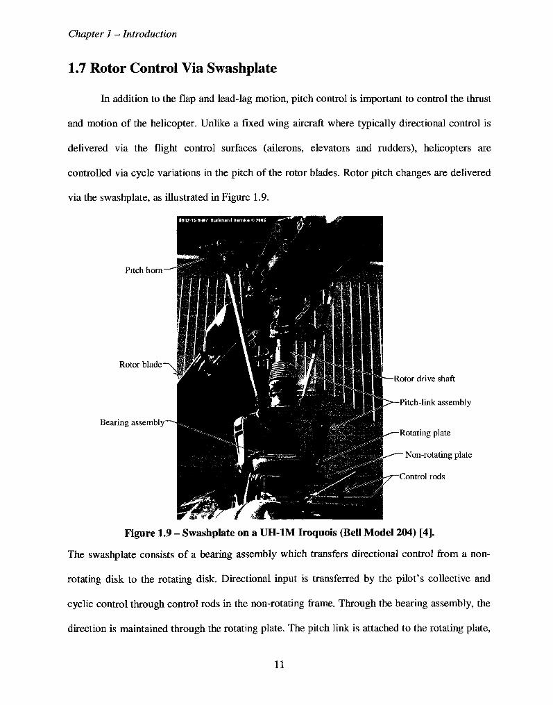
1.7 Rotor Control Via Swashplate
In addition to the flap and lead-lag motion, pitch control is important to control the thrust
and motion of the helicopter. Unlike a fixed wing aircraft where typically directional control is
delivered via the flight control surfaces (ailerons, elevators and rudders), helicopters are
controlled via cycle variations in the pitch of the rotor blades. Rotor pitch changes are delivered
via the swashplate, as illustrated in Figure 1.9.
Pitch horn
Rotor blade
Bearing assembly
Rotor drive shaft
Pitch-link assembly
Rotating plate
Non-rotating plate
Control rods
Figure 1.9 - Swashplate on a UH-1M Iroquois (Bell Model 204) [4].
The swashplate consists of a bearing assembly which transfers directional control from a non-
rotating disk to the rotating disk. Directional input is transferred by the pilot's collective and
cyclic control through control rods in the non-rotating frame. Through the bearing assembly, the
direction is maintained through the rotating plate. The pitch link is attached to the rotating plate,
11
Chapter 1 - Introduction
and delivers the change in pitch input to the pitch horn, which defines the final pitch of the blade.
For example as the pilot inputs an increase in collective pitch, the swashplate is pushed up, and
consequently tilts the blades upward, increasing the blades' angle of attack and Uft, enabling the
helicopter to climb up. Likewise, if the swashplate responds to the cyclic control, cyclical
changes to the pitch angle along the azimuth, enables the helicopter directional control in the
forward, aft, and left/right rolling directions. For a hinged rotor as in Figure 1.8 (b), the
swashplate influences the feathering hinge, which then controls the pitch of the blades.
With the many design options and configurations, it presents the opportunity for research
in 3D aeroelastic codes, the challenge for rotorcraft code developers is to create models that
provide a good representation of the dynamics that occur in the many helicopter systems.
1.8 Blade Elastic Deformation
It was shown that in forward flight, a helicopter blade experiences 3-degrees of freedom
(flap, lead-lag, pitch). Since the blade is a slender body, the blade itself elastically deforms
mostly in the flap and torsion directions. When designing the blade, one has to evaluate how the
blade will perform in the various helicopter flight regimes (forward flight, hover, ascent, descent,
etc.) and whether the blade will perform safely, efficiently and within the control of the pilot.
This requires rotorcraft code developers to model not only the aerodynamic environment but also
the blades' structural dynamics, their kinematics and their effects on the helicopter and
surrounding environment. Accounting for these additional effects may include calculating the
vibration loads occurring on the helicopter, the downstream rotor wake patterns, and
aeroacoustics. It is clear that developing such a simulation is a complex task, requiring
12
Chapter 1 - Introduction
sophisticated models from aerodynamics, structural dynamics, and blade kinematics points of
view.
At this point, there is no one single code which has the adequate sophistication in all
these areas. However, it is the work presented in this thesis that presents the expansion to the
SMARTROTOR rotorcraft model, by adding blade articulation and validating this model by
comparing simulation results to a series of wind tunnel test results.
1.9 Computational Aeroelastic Codes
Computational modeling of rotorcraft is used for evaluating new developments.
However, while rotorcraft testing, blade fabrication, etc., can be quite expensive, running
computational feasibility studies can provide a cost effective and timely solution to illustrate the
parameters and limits for new designs and testing. The challenge of these computational models
is their validation to how well they replicate the aerodynamic, dynamic and structural parameters
that effect the rotorcraft and its surrounding environment.
There are three comprehensive rotorcraft computational codes commercially available at
present. They are the DYMORE, CAMRAD II, and CHARM codes. DYMORE is a
comprehensive code that models multi-body structures through non-linear finite element
methods (FEM) of both hingeless and hinged blades [5]. The aerodynamic component consists of
two options. The first option is a built-in simple lifting-line and vortex method. The other option
allows for the user to couple a sophisticated computational fluid dynamics (CFD) module to
model the aerodynamics environment around the rotor at each time step. The second model,
CAMRAD II is a comprehensive aeromechanical model that can model geometrically complex
rotorcraft systems through a selection of several structural dynamic models [6]. The aerodynamic
13
Chapter 1 - Introduction
component consists of a 2nd-order lifting line theory and a sophisticated free wake geometry
model. CAMRAD II can model single, dual and tilt-rotor configurations, with articulated,
teetering, hingeless and bearingless hubs. The third model, CHARM is another comprehensive
model available, which can model the full complex fuselage body geometry of a helicopter [7].
The structural model consists of a simple finite element method to model the blade deformations,
for hinged and hingeless configurations. The aerodynamic model consists of a fast-panel and
fast-vortex method, designed to reduce the time and computational resources normally required
to model the complete helicopter configurations (including main rotor, tail rotor, and fuselage)
and interacting wake. Unlike DYMORE and CAMRAD II, the CHARM code has an
aeroacoustic model, allowing for the study of Blade Vortex Interaction (BVI) and rotor noise.
SMARTROTOR is the rotorcraft research modeling code used by the Rotorcraft
Research Group at Carleton University. As detailed later in Chapter 2, it consists of an
aerodynamic model, a structural model, and an aeroacoustic model. The structural model
consists of hingeless blades that deform based on Hodges non-linear deformation equations [8].
The aerodynamic model uses a coupled panel method and vortex method.
SMARTROTOR has some sophisticated features superior to the ones of DYMORE,
CAMRAD II or CHARM. These include the GENUVP aerodynamics module, the aeroacoustic
module, and the ability to model smart structures and active noise reduction technologies [8]. A
deficiency in SMARTROTOR is the absence of the articulated rotor hub model, i.e. the inability
to include hinges at the blade root. At present, SMARTROTOR consists of a hingeless hub
model based on Hodges' non-linear deformation equations, and a fixed rigid non-deforming
blade model used for wind turbine study. The work presented in this thesis therefore aims to add
14
Chapter 1 - Introduction
a simple rigid hinge model, as a step towards modeling the complex dynamics and kinematics of
an articulated hub with flexible blades.
1.10 Thesis Objectives
Based on the above review it is clear that in order to be able to design active rotor based
control systems, one needs a credible 3D aeroelastic code to predict the rotor aeromechanics. The
aeromechanics consists of the aerodynamics, dynamics, kinematics, and blade elasticity. The
SMARTROTOR code, though has an advanced aerodynamics model and blade elasticity model,
currently lacks the ability to model articulated hubs. Therefore, the objective of this thesis is to
introduce hinges or blade articulation into the SMARTROTOR code.
In particular, the following objectives were identified to achieve the overall goal:
1. Add a rigid blade articulated hub model.
2. Verify this model by comparing simulation results to the data from the Harris
experiment [9].
3. Complete the coupling of existing hingeless deformation code with an articulation
model.
1.11 Thesis Structure
Chapter 2 provides a background and history of the SMARTROTOR program. A
description of the aerodynamic module developed in the original wind turbine simulation
program GENUVP will be presented. Following this, the existing hingeless rotorcraft features,
created by Daniel Opoku and Tao Cheng are described [8] [10].
15
Chapter 1 - Introduction
Chapter 3 explains the construction of the rigid blade model, and the underlying theory
according to the Leishman equations of motion for rotor blades. The additions and amendments
to the SMARTROTOR code are explained.
Chapter 4 provides the results of the comparison of the rigid blade model to Franklin D
Harris' experiment on blade flapping motion [9]. This section illustrates that the simulations of
the rigid blade model correlate well with the wind tunnel results.
Chapter 5 contains a summary, concluding remarks, and recommendations of directions
for future work.
16
Chapter 2 - SMARTROTOR Background
Chapter 2 SMARTROTOR Background
This chapter summarizes the existing functionality of the SMARTROTOR program. Due
to the length and complexity of the preceding contributions, only the sections of the code that are
relevant to the current modeling work are described in detail. The SMARTROTOR program
consists of two distinct modules: the aerodynamic module and the structural module. From here
forward the term GENUVP will generally refer to the aerodynamic module, i.e. that portion of
the code that calculates the rotor blade aerodynamics and surrounding fluid environment. The
term STRUCTDEFORM will refer to the later part of the code that estimates the structural
deformation or displacement of the rotor blades.
2.1 GENUVP Overview
The aerodynamic component of SMARTROTOR was created from the GENeral
Unsteady Vortex Particle (GENUVP) Fortran 77 code. It was developed by Prof. Spyros G.
Voutsinas and his team at the National Technical University of Athens, Greece [11]. It consists
of a panel method to calculate the blade aerodynamics loads and a discrete vortex method, which
generates the aerodynamic wake environment. The wake model estimates the path and rotations
of the vortex particles shedding off the blades, predicts their paths through the fluid environment,
and interaction with the adjacent blades. The code is essentially grid-free, enabling easy
modeling of mutually moving rigid bodies, such as that of a rotating rotor. Details of GENUVP
are found in references [12] and [13], and is also summarized in Daniel Opoku's Thesis on
Aeroelastic and Aeroacoustic Modelling of Rotorcraft [8]. A brief explanation of GENUVP is as
follows:
17
Chapter 2 - SMARTROTOR Background
The GENUVP aerodynamic environment is based on the Helmholtz decomposition,
which states that any velocity field, u can be represented by a irrotational part usoUd and a
rotational part uwake [13]. The aerodynamic flowfield is decomposed as a function of position
and time where:
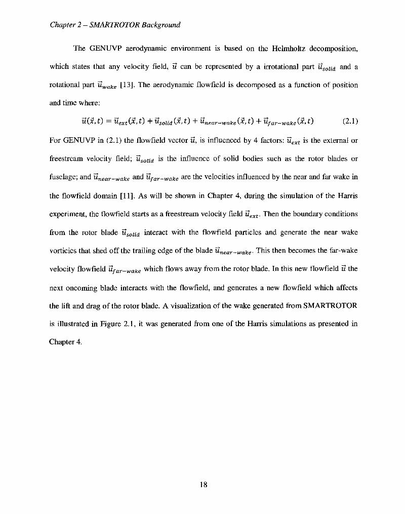
U[X,t) = Uext(X,t) +Us0U(i\X,t) + Unear-wafceC^» tJ + ufar~wake\x> tJ (2-1)
For GENUVP in (2.1) the flowfield vector u, is influenced by 4 factors: uext is the external or
freestream velocity field; usoUd is the influence of solid bodies such as the rotor blades or
fuselage; and unear^wake and Ufar_wake are the velocities influenced by the near and far wake in
the flowfield domain [11]. As will be shown in Chapter 4, during the simulation of the Harris
experiment, the flowfield starts as a freestream velocity field uext. Then the boundary conditions
from the rotor blade usoUd interact with the flowfield particles and generate the near wake
vorticies that shed off the trailing edge of the blade Unear-wake • This then becomes the far-wake
velocity flowfield Ufar-wake which flows away from the rotor blade. In this new flowfield u the
next oncoming blade interacts with the flowfield, and generates a new flowfield which affects
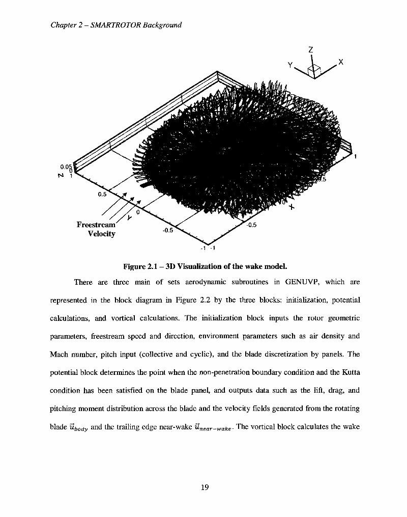
the lift and drag of the rotor blade. A visualization of the wake generated from SMARTROTOR
is illustrated in Figure 2.1, it was generated from one of the Harris simulations as presented in
Chapter 4.
18
Chapter 2 - SMARTROTOR Background
There are three main of sets aerodynamic subroutines in GENUVP, which are
represented in the block diagram in Figure 2.2 by the three blocks: initialization, potential
calculations, and vortical calculations. The initialization block inputs the rotor geometric
parameters, freestream speed and direction, environment parameters such as air density and
Mach number, pitch input (collective and cyclic), and the blade discretization by panels. The
potential block determines the point when the non-penetration boundary condition and the Kutta
condition has been satisfied on the blade panel, and outputs data such as the lift, drag, and
pitching moment distribution across the blade and the velocity fields generated from the rotating
blade ubody and the trailing edge near-wake unear^wake. The vortical block calculates the wake
19
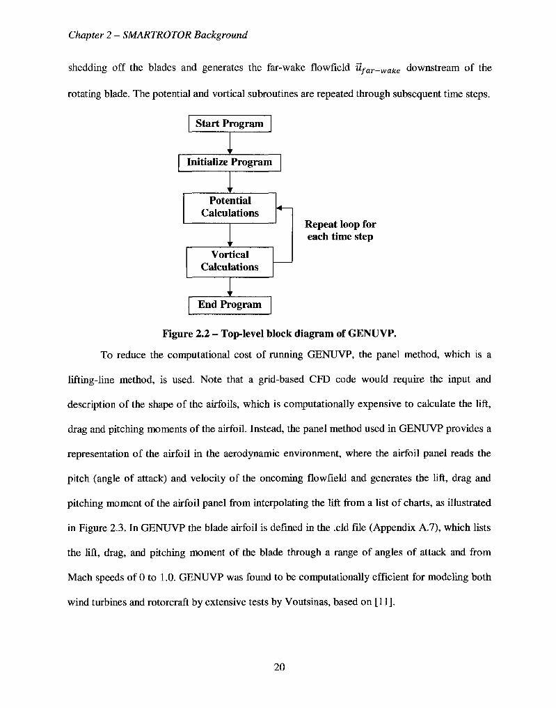
Chapter 2 - SMARTROTOR Background
shedding off the blades and generates the far-wake flowfield Ufar_wake downstream of the
rotating blade. The potential and vortical subroutines are repeated through subsequent time steps.
Start Program
V
Initialize Program
y
Potential Calculations
i r
Vortical Calculations
1 ' End Program
Repeat loop for each time step
Figure 2.2 - Top-level block diagram of GENUVP.
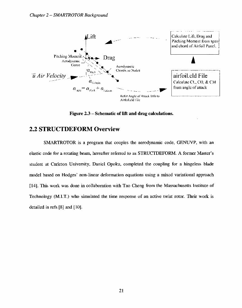
To reduce the computational cost of running GENUVP, the panel method, which is a
lifting-line method, is used. Note that a grid-based CFD code would require the input and
description of the shape of the airfoils, which is computationally expensive to calculate the lift,
drag and pitching moments of the airfoil. Instead, the panel method used in GENUVP provides a
representation of the airfoil in the aerodynamic environment, where the airfoil panel reads the
pitch (angle of attack) and velocity of the oncoming flowfield and generates the lift, drag and
pitching moment of the airfoil panel from interpolating the lift from a list of charts, as illustrated
in Figure 2.3. In GENUVP the blade airfoil is defined in the .eld file (Appendix A.7), which lists
the lift, drag, and pitching moment of the blade through a range of angles of attack and from
Mach speeds of 0 to 1.0. GENUVP was found to be computationally efficient for modeling both
wind turbines and rotorcraft by extensive tests by Voutsinas, based on [11].
20
Chapter 2 - SMARTROTOR Background
Pitch im; Moment,
Lift
Aerodynamic Centre
;H^*~ Drag
li Air Velocity
x x • <'\ X x
\aPitch X -xH(
Aerodynamic Chordw ise Nodes
x v .
a!\'hcsn-
^WA ® rmh a Idiot m
Refer Angle of Attack Info to Airtbil.cld File
Calculate Lift, Drag and Pitching Moment from span and chord of Airfoil Panel.
airfoil.eld File Calculate CL, CD, & CM from angle of attack
Figure 2.3 - Schematic of lift and drag calculations.
2.2 STRUCTDEFORM Overview
SMARTROTOR is a program that couples the aerodynamic code, GENUVP, with an
elastic code for a rotating beam, hereafter referred to as STRUCTDEFORM. A former Master's
student at Carleton University, Daniel Opoku, completed the coupling for a hingeless blade
model based on Hodges' non-linear deformation equations using a mixed variational approach
[14]. This work was done in collaboration with Tao Cheng from the Massachusetts Institute of
Technology (M.I.T.) who simulated the time response of an active twist rotor. Their work is
detailed in refs [8] and [10].
21
Chapter 2 - SMARTROTOR Background
-HINGELESS ROTORS-Blade Attachment
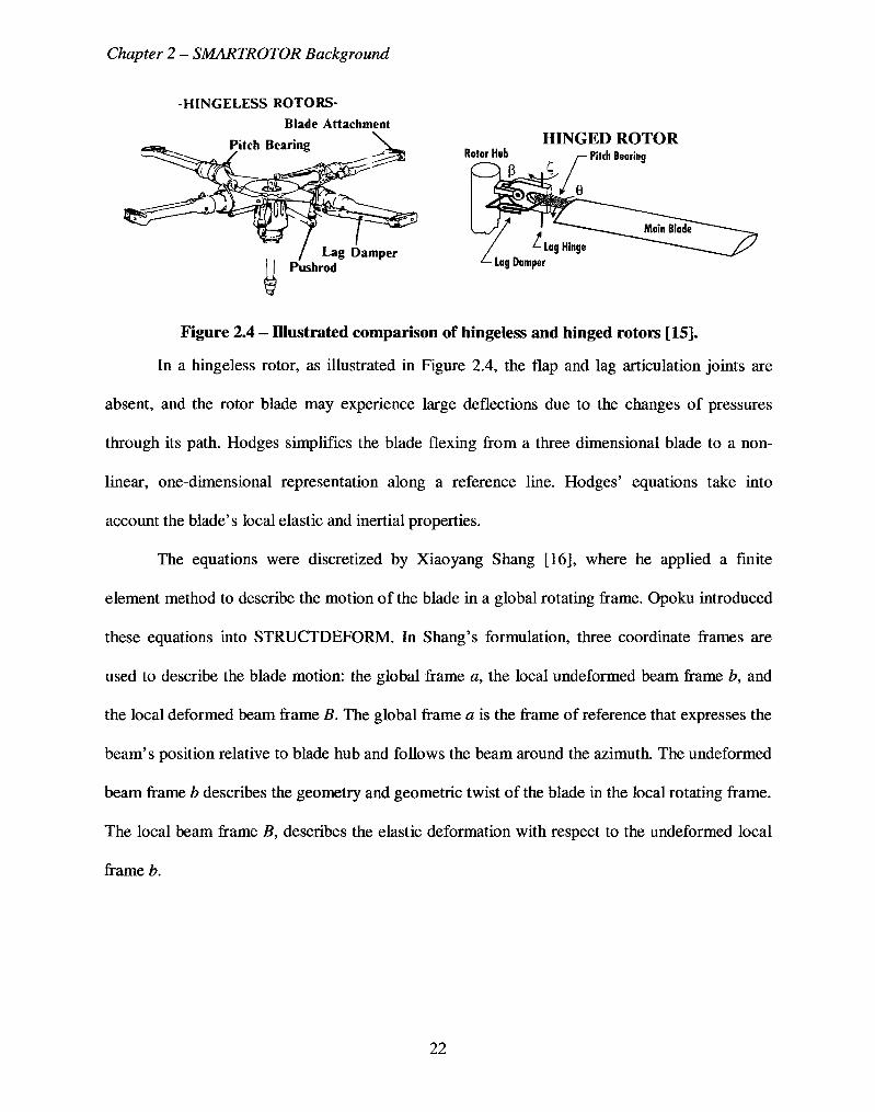
Figure 2.4 - Illustrated comparison of hingeless and hinged rotors [15].
In a hingeless rotor, as illustrated in Figure 2.4, the flap and lag articulation joints are
absent, and the rotor blade may experience large deflections due to the changes of pressures
through its path. Hodges simplifies the blade flexing from a three dimensional blade to a non
linear, one-dimensional representation along a reference line. Hodges' equations take into
account the blade's local elastic and inertial properties.
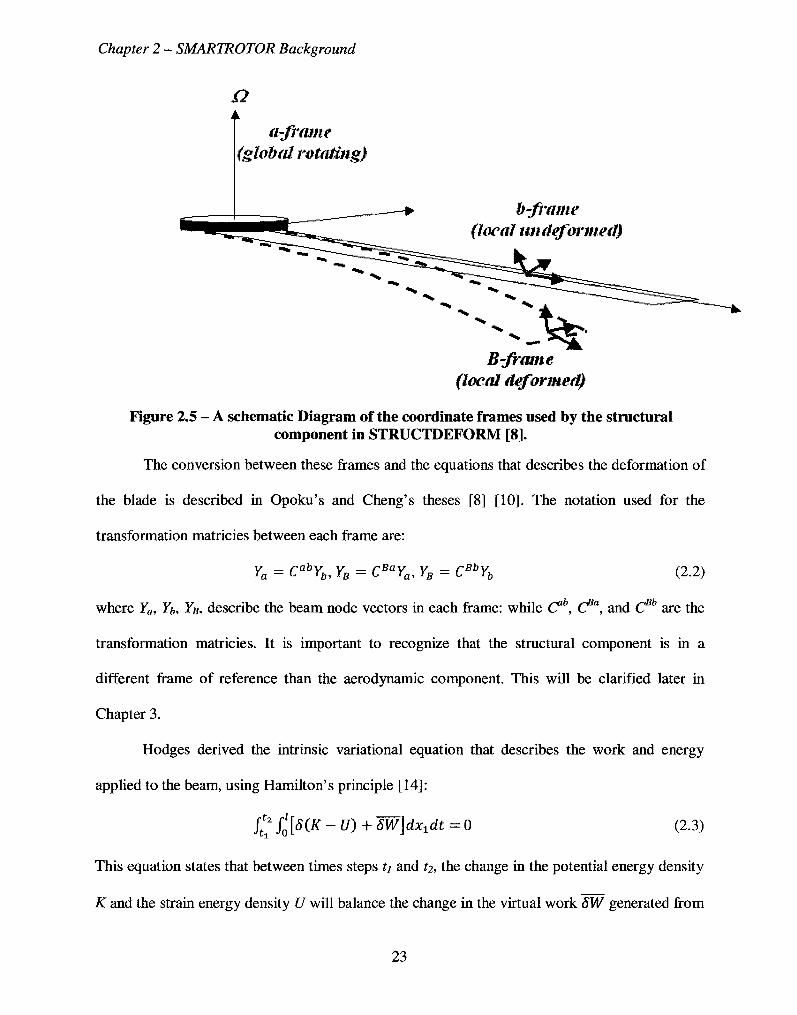
The equations were discretized by Xiaoyang Shang [16], where he applied a finite
element method to describe the motion of the blade in a global rotating frame. Opoku introduced
these equations into STRUCTDEFORM. In Shang's formulation, three coordinate frames are
used to describe the blade motion: the global frame a, the local undeformed beam frame b, and
the local deformed beam frame B. The global frame a is the frame of reference that expresses the
beam's position relative to blade hub and follows the beam around the azimuth. The undeformed
beam frame b describes the geometry and geometric twist of the blade in the local rotating frame.
The local beam frame B, describes the elastic deformation with respect to the undeformed local
frame b.
22
Chapter 2 - SMARTROTOR Background
Q A
a-frame (global rotating}
B-fmrne (local deformed)
Figure 2.5 - A schematic Diagram of the coordinate frames used by the structural component in STRUCTDEFORM [8].
The conversion between these frames and the equations that describes the deformation of
the blade is described in Opoku's and Cheng's theses [8] [10]. The notation used for the
transformation matricies between each frame are:
Ya = CabYb, YB = CBaYa, YB = CBbYb (2.2)
where Ya, Yb, YB, describe the beam node vectors in each frame: while Cb, (fa, and CBh are the
transformation matricies. It is important to recognize that the structural component is in a
different frame of reference than the aerodynamic component. This will be clarified later in
Chapter 3.
Hodges derived the intrinsic variational equation that describes the work and energy
applied to the beam, using Hamilton's principle [14]:
Jt' /o t 5 ( i f ~ y ) + SW\dxxdt = 0 (2.3)
This equation states that between times steps t\ and t2, the change in the potential energy density
K and the strain energy density U will balance the change in the virtual work SW generated from
23
Chapter 2 - SMARTROTOR Background
the applied loads. For a detailed description of mixed formulation refer again to Opoku's and
Cheng's theses [8] [10].
The next section of interest is the discretized equations, which solves for the beams
equations of motion:
g8Xr[Fs(X,i)]dt = 0 (2.4)
Here, Fs is the matrix operator containing the beam's complete non-linear equations of motion. X
is the vector that contains the unknown measures of displacement, rotation, internal loads,
momenta, and energies, of each spanwise node from 1 to node N, and includes the unknown
boundary values. SXT is the change of the X vector from time ti to time fc, and the superscript T
denotes the matrix transpose. Dot denotes the time differential. The X vector describes the
structural state of the rotor blade, in terms of the local nodal variables. It takes the form:
X = [PmulBlFlMlPlHl ...ulelFXPlHlul^SlJ (2.5)
where the nodal measures are as follows: F is the internal force vector, M is the internal moment
vector, u is the displacement measure (the nodal deformation from the undeformed frame), 6 is
the angular orientation measure, P is the linear momentum vector, and H is the angular
momentum vector. The boundary conditions are also described in the X vector; in this case
presented for the hingeless blade condition. At the root, F[ and Ml are the unknown internal
force and moment vectors, respectively. At the blade tip, at node location N+l, ujj+1 and #jv+1
are the unknown displacement and angular orientation measures. Also note that for the hingeless
rotor at the root, the root nodal displacement and angles measures are ux = 0 and 6t = 0, and at
the blade tip the internal forces and moments FN+l = 0 and Mw+1 = 0 equal zero.
The structural deformation code solves the preceding non-linear equations of motion. The
solver was developed by Tao Cheng [10], and was based on the discretization of Shang's
24
Chapter 2 - SMARTROTOR Background
formulation [16]. The integration of the equations is accomplished by a second-order Euler
method, and then the X vector of unknowns is solved iteratively by using the Newton-Raphson
method.
Opoku validated his hingeless model against the HELINOISE test results. The
HELINOISE (synonym for helicopter external noise) test program was a series of detailed
hingeless rotor blade tests conducted at the German-Dutch Wind Tunnel (DNW) in 1990 [17].
Details of the hingeless model can be found is Opoku's thesis [8]. This thesis will not discuss
much more concerning the hingless model. Instead, references to the hingeless model will be
concerned with its decoupling structural subroutines from the GENUVP aerodynamics model,
and its replacement with the subroutines to run the hinged rigid model.
25
Chapter 3 - Rotating Rigid Blade Model
Chapter 3 Rotating Rigid Blade Model
As discussed in Chapter 2, the current version of SMARTROTOR originally began as a
rigid aerodynamic wind turbine code called GENUVP. Then, a hingeless aeroelastic model,
STRCUTDEFORM was added to create SMARTROTOR. This chapter presents the addition of
new subroutines to SMARTROTOR by this author to calculate the flap and lead-lag motions of
hinged rigid rotor blades, and coupling them with the aerodynamic code. The previous hingeless
aeroelastic structural code, STRUCTDEFORM is turned off when the hinged rigid model is run.
The verification of this model is presented in Chapter 4, where a series of simulations are
compared to the experimental results presented in Franklin D. Harris' experiment [9].
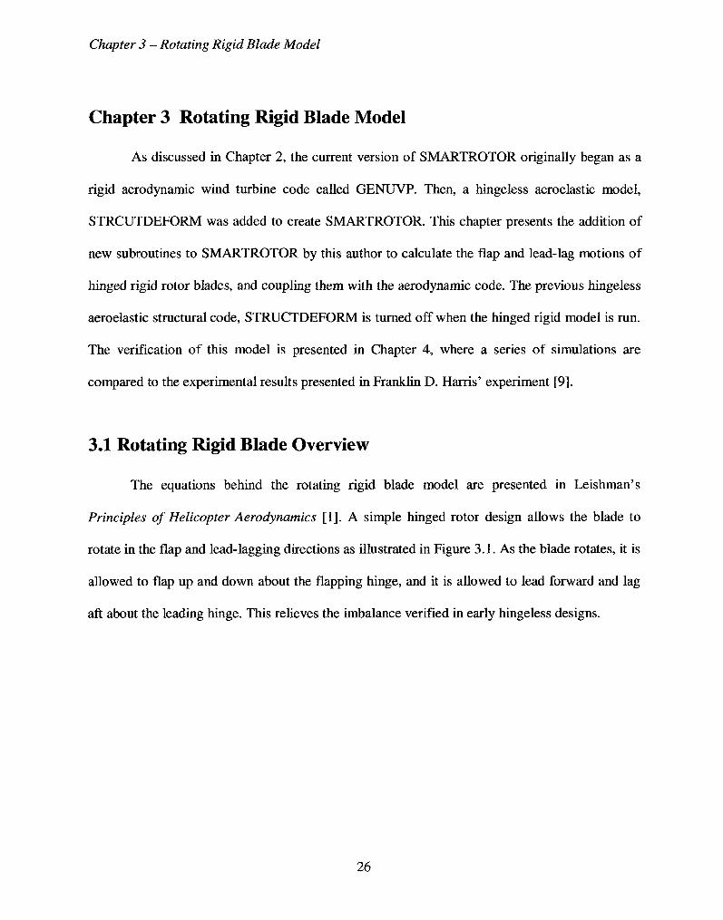
3.1 Rotating Rigid Blade Overview
The equations behind the rotating rigid blade model are presented in Leishman's
Principles of Helicopter Aerodynamics [1]. A simple hinged rotor design allows the blade to
rotate in the flap and lead-lagging directions as illustrated in Figure 3.1. As the blade rotates, it is
allowed to flap up and down about the flapping hinge, and it is allowed to lead forward and lag
aft about the leading hinge. This relieves the imbalance verified in early hingeless designs.
26
Chapter 3 - Rotating Rigid Blade Model
^otalwraal axis
Lead/teg , a a w
Tom lift
,1
Tatell drag fare®
Lsadung
Legging
FHapjsifigi (town
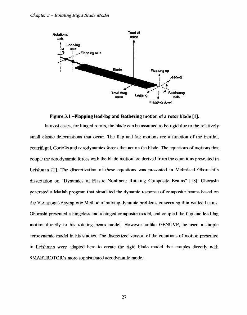
Figure 3.1 -Flapping lead-lag and feathering motion of a rotor blade [1].
In most cases, for hinged rotors, the blade can be assumed to be rigid due to the relatively
small elastic deformations that occur. The flap and lag motions are a function of the inertial,
centrifugal, Coriolis and aerodynamics forces that act on the blade. The equations of motions that
couple the aerodynamic forces with the blade motion are derived from the equations presented in
Leishman [1]. The discretization of these equations was presented in Mehrdaad Ghorashi's
dissertation on "Dynamics of Elastic Nonlinear Rotating Composite Beams" [18]. Ghorashi
generated a Matlab program that simulated the dynamic response of composite beams based on
the Variational-Asymptotic Method of solving dynamic problems concerning thin-walled beams.
Ghorashi presented a hingeless and a hinged composite model, and coupled the flap and lead-lag
motion directly to his rotating beam model. However unlike GENUVP, he used a simple
aerodynamic model in his studies. The discretized version of the equations of motion presented
in Leishman were adapted here to create the rigid blade model that couples directly with
SMARTROTOR's more sophisticated aerodynamic model.
27
Chapter 3 - Rotating Rigid Blade Model
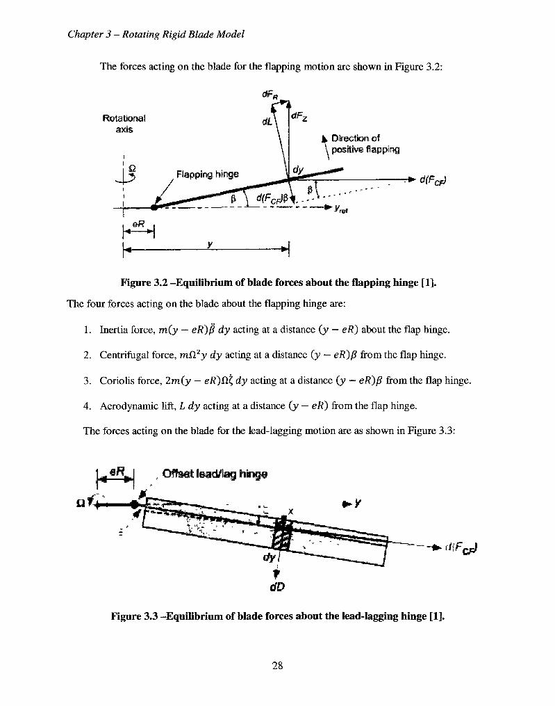
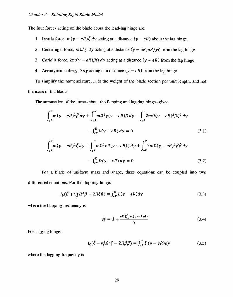
The forces acting on the blade for the flapping motion are shown in Figure 3.2:
Rotational axis
%, Direction! of \ positive flapping
*HFcJ
eR * *>
Figure 3.2 -Equilibrium of blade forces about the flapping hinge [1].
The four forces acting on the blade about the flapping hinge are:
1. Inertia force, m(y — eR)R dy acting at a distance (y — eR) about the flap hinge.
2. Centrifugal force, mD.2y dy acting at a distance (y — eR)(3 from the flap hinge.
3. Coriolis force, 2m(y — eR)Q.t, dy acting at a distance (y — eR)p from the flap hinge.
4. Aerodynamic lift, L dy acting at a distance (y — eR) from the flap hinge.
The forces acting on the blade for the lead-lagging motion are as shown in Figure 3.3:
Offset lead/lag hinge
tf^cp'
Figure 3.3 -Equilibrium of blade forces about the lead-lagging hinge [1].
28
Chapter 3 - Rotating Rigid Blade Model
The four forces acting on the blade about the lead-lag hinge are:
1. Inertia force, m(y — eR)( dy acting at a distance (y — eR) about the lag hinge.
2. Centrifugal force, mfl2y dy acting at a distance (y — eR)eR/y^ from the lag hinge.
3. Coriolis force, 2m(y — eR)RD. dy acting at a distance (y — eR) from the lag hinge.
4. Aerodynamic drag, D dy acting at a distance (y — eR) from the lag hinge.
To simplify the nomenclature, m is the weight of the blade section per unit length, and not
the mass of the blade.
The summation of the forces about the flapping and lagging hinges give:
/• R r R r R
\ m(y - eR)2'$ dy + I mtfyiy - eR)B dy - J 2mn(y - eR)2R^2 dy JeR JeR JeR
-f*RL(y-eR)dy = 0 (3.1)
/•R rR rR
I m(y - eR)2'(dy + I mQ.2eR(y - eR)(, dy + I 2mfl(y - eR)2p$ dy JeR 'eR •'eR
-J*RD(y-eR)dy = 0 (3.2)
For a blade of uniform mass and shape, these equations can be coupled into two
differential equations. For the flapping hinge:
Ib0 + vjn2{$ - 2n(P) = jeR
R L(y - eR)dy (3.3)
where the flapping frequency is
+ « * J > f r - R ) 4 y
For lagging hinge:
Itf + v2!22<; - 21200) = J*RD(y- eR)dy (3.5)
where the lagging frequency is
29
Chapter 3 - Rotating Rigid Blade Model
2 _ eRSeRm(y-eR)dy (3.6)
In the present work, these equations are discretized and introduced in the subroutine
BLADEARTICULATE, located in the file bladeartic.f (Appendix B.4).
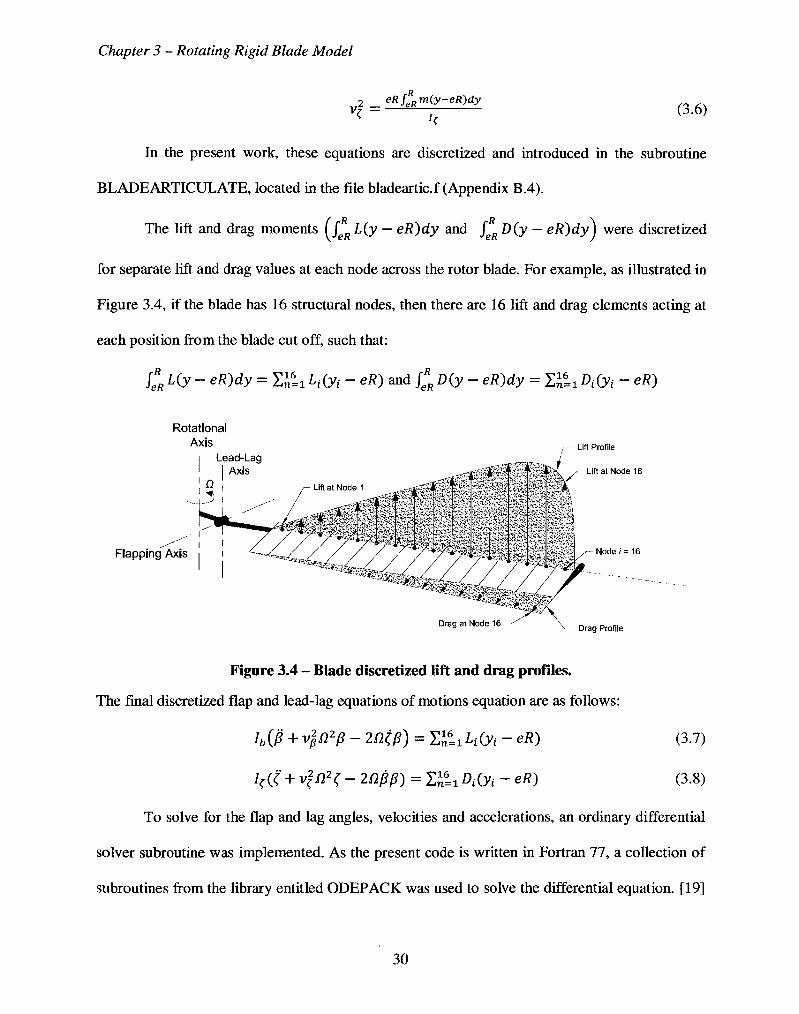
The lift and drag moments (jgR L(y - eR)dy and fgR D(y — eR)dyj were discretized
for separate lift and drag values at each node across the rotor blade. For example, as illustrated in
Figure 3.4, if the blade has 16 structural nodes, then there are 16 lift and drag elements acting at
each position from the blade cut off, such that:
/ * L(y - eR)dy = J^U Lt(yt - eR) and J* D(y - eR)dy = Y£=1 Di(yt - eK)
Rotational Axis
I Lead-Lag I | Axis
Q
Flapping Axis Node/= 16
— Drag Profile
Figure 3.4 - Blade discretized lift and drag profiles.
The final discretized flap and lead-lag equations of motions equation are as follows:
Ib(p + v}n2(S - 2/2#) = ntik&i - e^ (3.7)
/f (C + v|/22C - 21200) = nU Didyi - eR) (3.8)
To solve for the flap and lag angles, velocities and accelerations, an ordinary differential
solver subroutine was implemented. As the present code is written in Fortran 77, a collection of
subroutines from the library entitled ODEPACK was used to solve the differential equation. [19]
30
Chapter 3 - Rotating Rigid Blade Model
The code for solving the flap and lead-lag angles are found in subroutine
BLADEARTICULATE, located in file bladeartic.f. Refer to the code in Appendix B.5 for the
method of setting up the ODEPACK subroutines.
3.2 Coupling Rigid Motion with Aerodynamics
With the flap and lead-lag subroutines complete, interpolation subroutines were created
to rotate the aerodynamic nodes along the azimuth position. Opoku's version of SMARTROTOR
calculates the structural deformation of hingeless rotor blades, as described in Chapter 2. In this
case, the rigid blade model is assumed, and the structural deformation subroutines were turned
off.
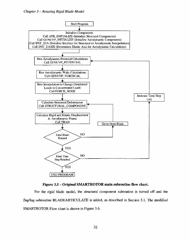
The main program that runs SMARTROTOR is located in the file COMBINED_C.f.
Refer to Appendix B.l for this code. The flow chart of the main subroutine follows, in Figure
3.5.
31
Chapter 3 - Rotating Rigid Blade Model
Start Program
Initialize Components Call ATRjNTTIALIZE (Initialize Structural Components)
Call GENUVP_INITIALIZE (Initialize Aerodynamic Components) Call INTTJS2A (Initialize Interface for Structural to Aerodynamic Interpolation)
Call INTT_EAXIS (Determines Elastic Axis for Aerodynamic Calculations)
Run Aerodynamic Potential Calculations Call GENUVP POTENTIAL
I Run Aerodynamic Wake Calculations
Call GENUVP VORTICAL
Run Interpolation to Change Distributed Loads to Concentrated Loads
Call FORCE NODE
Calculate Structural Deformation Call STRUCTURAL_COMPONENT
I Calculate Rigid and Elastic Displacement
in Aerodynamic Frame Call TRAN
END PROGRAM
Increase Time Step (At)
Go to Next Blade
Figure 3.5 - Original SMARTROTOR main subroutine flow chart.
For the rigid blade model, the structural component subroutine is turned off and the
flap/lag subroutine BLADE ARTICULATE is added, as described in Section 3.1. The modified
SMARTROTOR Flow chart is shown in Figure 3.6.
32

Chapter 3 — Rotating Rigid Blade Model
Start Program
Initialize Components Call ATRJMTIALIZE (Initialize Structural Components)
Call GENUVP_INITIALIZE (Initialize Aerodynamic Components) Call INIT_S2A (Initialize Interface for Structural to Aerodynamic Interpolation)
Call INTT_EAXIS (Determines Elastic Axis for Aerodynamic Calculations)
Run Aerodynamic Potential Calculations Call GENUVP_POTENTIAL
I Run Aerodynamic Wake Calculations
Call GENUVPJVORTICAL
Run Interpolation to Change Distributed Loads to Concentrated Loads
Call FORCE NODE
Calculate Flap and Lead-Lag Angle and Velocities Call BLADEARTICULATE
Calculate Rigid and Elastic Displacement in Aerodynamic Frame
Call TRAN
Increase Time Step (At)
Go to Next Blade
NO
NO
END PROGRAM
Figure 3.6 - Modified SMARTROTOR main subroutine flow chart
To maintain the accuracy of the interpolation, some subroutines from Opoku's
SMARTROTOR were modified. These modifications are presented in the following sections.
33
Chapter 3 - Rotating Rigid Blade Model
3.3 Interpolation from Aerodynamic Model to Rigid Blade Model
The lift and drag values are collected from the subroutine TNWEAOA, located in rescpv-
3_sp.coupled2.f. This subroutine corrects the viscous effect for thin wings based on the effective
angle of attack. As the initialization requires an equal number of spanwise aerodynamic and
structural nodes, it is simple to assign them, with the addition of instructions below in the
TNWEAOA subroutine, located after the calculation of the lift, drag and pitching moment:
DRAG = G_den*0.5*AIRDEN*CHRDL*BSEC*CD*VMAG**2 '.Drag Node Calculation RLIF = G_den*0.5*AIRDEN*CHRDL*BSEC*CL*VMAG**2 '.Lift Node Calculation PMOM = G_den*0.5*AIRDEN*CHRDL*CHRDL*BSEC*CM*VMAG**2 !Pitching Moment
C Directly assigning Lift and Drag for Articulation Subroutine c
IF (IARTIC.EQ.l) THEN !When Articulation is Activated ARTICLIFT (J, NB) = RLIF '.Assigning Lift at span node J, blade NB ARTICDRAG (J, NB) = DRAG '.Assigning Drag at span node J, blade NB
END IF c
Then the lift and drag variables are recalled in the subroutine BLADEARTICULATE, as
described in Section 3.1. In the above, the ARTICLIFT and ARTICDRAG are the arrays that
store the nodal lift and drag magnitudes for each node index J, and blade number NB.
3.4 Interpolation from Rigid Blade Model to Aerodynamic Model
From subroutine BLADEARTICULATE, the flap and lead-lag angles and velocities are
sent to subroutine TRAN. Subroutine TRAN, located in file couple.f, calculates the new
positions of the aerodynamic blade nodes (Appendix B.6). Normally it would have generated the
displaced position of the structure nodes from subroutine STRUCTURAL_COMPONENT,
located in file couple.f. However, for the rigid model, subroutine
34
Chapter 3 - Rotating Rigid Blade Model
STRUCTURAL_COMPONENT is turned off, and the TRAN subroutine was modified to
displace new positions of the structure nodes with respect to only the flap and lead-lag angles.
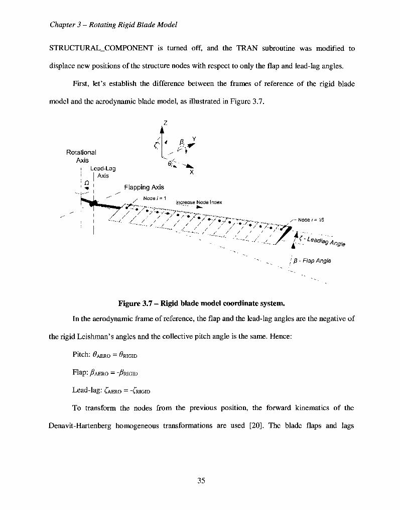
First, let's establish the difference between the frames of reference of the rigid blade
model and the aerodynamic blade model, as illustrated in Figure 3.7.
Rotational Axis
I Lead-Lag ! I Axis ! fl
c
9v
Flapping Axis
v Node i - 1 y Increase Node Index
/ / / / * / » / - • / „ ? Node/ =16
/ / / / / / ^--Lead,a9Angle
I ft - Flap Angle
Figure 3.7 - Rigid blade model coordinate system.
In the aerodynamic frame of reference, the flap and the lead-lag angles are the negative of
the rigid Leishman's angles and the collective pitch angle is the same. Hence:
Pitch: #AERO - FRIGID
Flap: /?AERO = -/FRIGID
Lead-lag: CAERO = -CRIGID
To transform the nodes from the previous position, the forward kinematics of the
Denavit-Hartenberg homogeneous transformations are used [20]. The blade flaps and lags
35
Chapter 3 - Rotating Rigid Blade Model
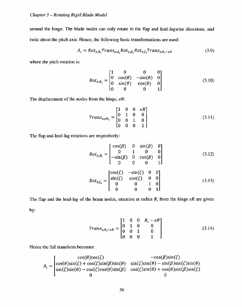
around the hinge. The blade nodes can only rotate in the flap and lead-lagwise directions, and
twist about the pitch axis. Hence, the following basic transformations are used:
At = RotxeTransx>dRotySRotz><;TransZiRi_eR (3.9)
where the pitch rotation is:
Rotx>6i =
1 0 0 0 0 cos(0) -sin(0) 0 0 sin(0) cos(0) 0 0 0 0 1.
(3.10)
The displacement of the nodes from the hinge, eR:
TransXi6Ri
1 0 0 eR 0 1 0 0 0 0 1 0 0 0 0 1
(3.11)
The flap and lead-lag rotations are respectively:
Rot y.Px
Rot*Ax =
cos(/?) 0 sin(/?) 0 0 1 0 0
-sin(/?) 0 cos(/?) 0 0 0 0 1.
cos(0 - s i n ( 0 0 0 sin(0 cos(<") 0 0
0 0 1 0 0 0 0 1
(3.12)
(3.13)
The flap and the lead-lag of the beam nodes, situation at radius R, from the hinge eR are given
by:
TranszRi-eR —
1 0 0 Rt-eR 0 1 0 0 0 0 1 0
L0 0 0 1
(3.14)
Hence the full transform becomes:
A =
cos(0)cos«") -cos(/?)sin(0 cos(0)sin(O + cos(<")sin(^)sin(0) sin(Ocos(0) - sin()S)sin(Osin(0) sin(Osin(0) - cos«")cos(0)sin(/5) cos(Osin(0) + cos(0)sin(/?)sin(O
0 0
36
Chapter 3 - Rotating Rigid Blade Model
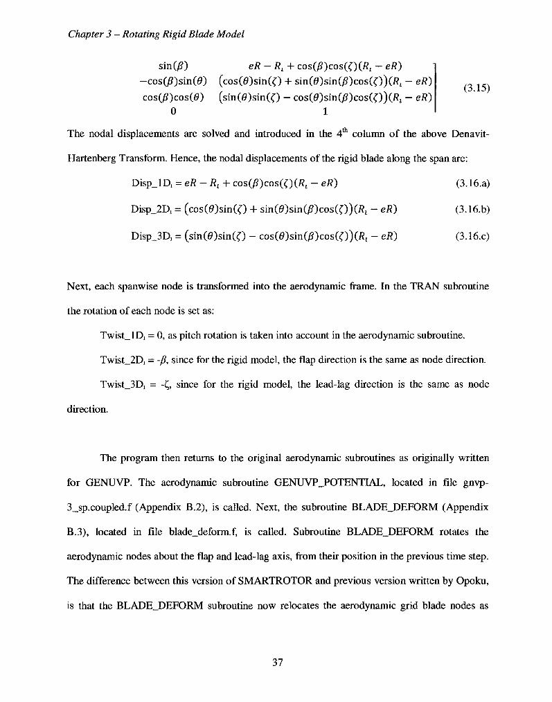
sinQ?) eR-Rl + cos(/?)cos(0(/?t - eJ?)
-cos(/?)sin(0) (cos(0)sin(O + sin(0)sin(/?)cos(O)(#i - eR)
cos(/?)cos(0) (sin(0)sin(O - cos(0)sinO3)cos(O)(#t - eR) 0 1
The nodal displacements are solved and introduced in the 4th column of the above Denavit-
Hartenberg Transform. Hence, the nodal displacements of the rigid blade along the span are:
Disp_lD1 = eR - Rt + cos(/?)cos(0(/?l - eR) (3.16.a)
Disp_2D, = (cos(e)sin(O + sin(0)sin(/?)cos(O)(fli - eR) (3.16.b)
Disp_3D, = (sin(0)sin(O - cos(0)sin(/?)cos«'))(^l - eR) (3.16.c)
Next, each spanwise node is transformed into the aerodynamic frame. In the TRAN subroutine
the rotation of each node is set as:
Twist_lD, = 0, as pitch rotation is taken into account in the aerodynamic subroutine.
Twist_2Di = -/?, since for the rigid model, the flap direction is the same as node direction.
TwisOD; = -£, since for the rigid model, the lead-lag direction is the same as node
direction.
The program then returns to the original aerodynamic subroutines as originally written
for GENUVP. The aerodynamic subroutine GENUVP_POTENTIAL, located in file gnvp-
3_sp.coupled.f (Appendix B.2), is called. Next, the subroutine BLADE_DEFORM (Appendix
B.3), located in file blade_deform.f, is called. Subroutine BLADE_DEFORM rotates the
aerodynamic nodes about the flap and lead-lag axis, from their position in the previous time step.
The difference between this version of SMARTROTOR and previous version written by Opoku,
is that the BLADE_DEFORM subroutine now relocates the aerodynamic grid blade nodes as
37
Chapter 3 - Rotating Rigid Blade Model
defined by the new flap and lead-lag angles, while the previous version relocated the blade nodes
as per the deformed structure of the hingeless blade.
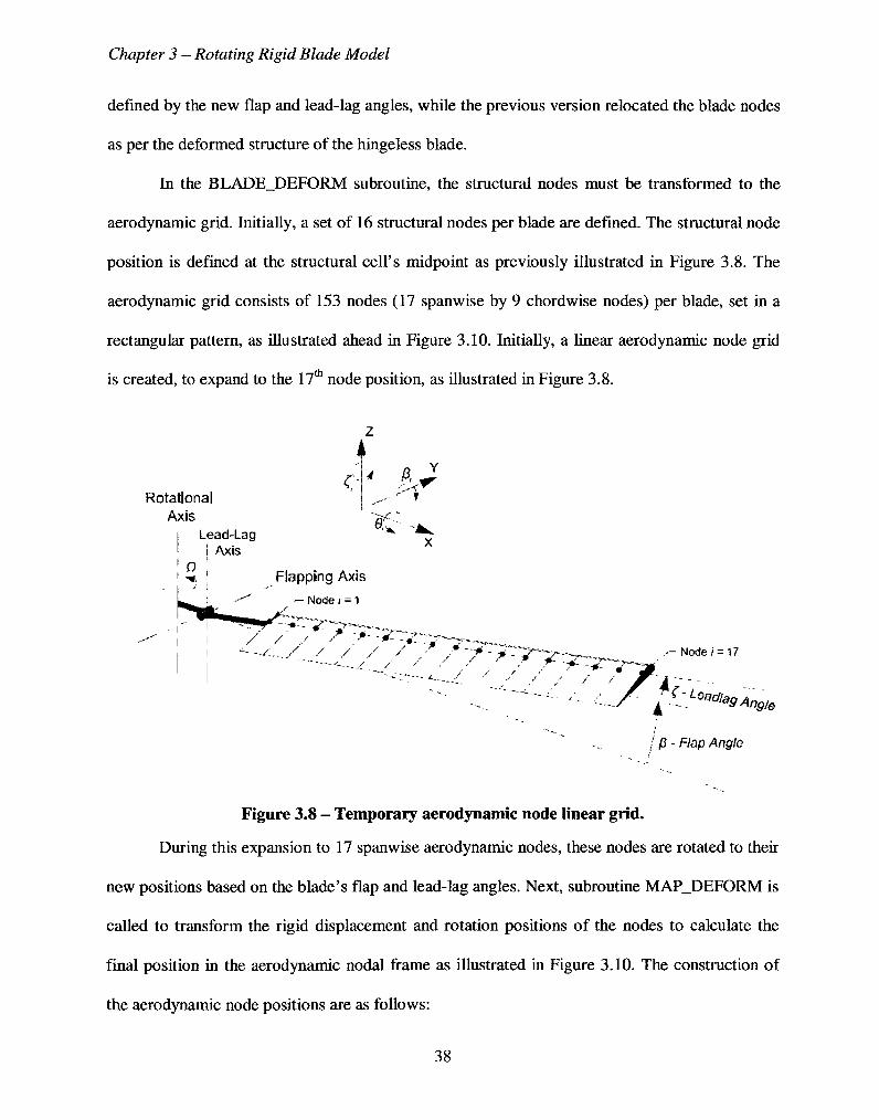
In the BLADE_DEFORM subroutine, the structural nodes must be transformed to the
aerodynamic grid. Initially, a set of 16 structural nodes per blade are defined. The structural node
position is defined at the structural cell's midpoint as previously illustrated in Figure 3.8. The
aerodynamic grid consists of 153 nodes (17 spanwise by 9 chordwise nodes) per blade, set in a
rectangular pattern, as illustrated ahead in Figure 3.10. Initially, a linear aerodynamic node grid
is created, to expand to the 17th node position, as illustrated in Figure 3.8.
Z
C Rotational
4 A J ' T
Axis x . Lead-Lag ' ^
Axis
Flapping Axis
N o d e i = 1
I I •"—-'— / / / / / - / ~~?-~*^r~T~-~~.— r-Node/ = 17
I p - Flap Angle
Figure 3.8 - Temporary aerodynamic node linear grid.
During this expansion to 17 spanwise aerodynamic nodes, these nodes are rotated to their
new positions based on the blade's flap and lead-lag angles. Next, subroutine MAP_DEFORM is
called to transform the rigid displacement and rotation positions of the nodes to calculate the
final position in the aerodynamic nodal frame as illustrated in Figure 3.10. The construction of
the aerodynamic node positions are as follows:
38
Chapter 3 - Rotating Rigid Blade Model
DISP(xaero)i = -i(DISP(y s t r u c t)i + DISP(ystruct)i+1) (3.17.a)
DISP(yaero)i = \ (DISP(xstruct)i + DISP(xstruct)i+1) (3.17.b)
DISP(zaero)i = ^(DISPCzstraOi + DISPCzstrat)^) (3.17.C)
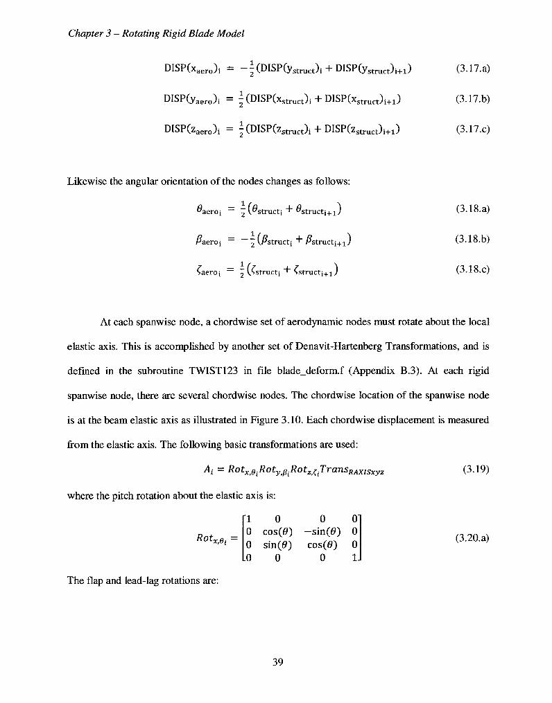
Likewise the angular orientation of the nodes changes as follows:
^aeroj = 2 V^struct; + ^structj+iJ (3.18.a)
Paeroj = — ^ IPstructj + Pstructj+1J (3.18.b)
Caeroi = 2 v^structj + Sstructj+1J (3.18.C)
At each spanwise node, a chordwise set of aerodynamic nodes must rotate about the local
elastic axis. This is accomplished by another set of Denavit-Hartenberg Transformations, and is
defined in the subroutine TWIST123 in file blade_deform.f (Appendix B.3). At each rigid
spanwise node, there are several chordwise nodes. The chordwise location of the spanwise node
is at the beam elastic axis as illustrated in Figure 3.10. Each chordwise displacement is measured
from the elastic axis. The following basic transformations are used:
At =RotXie.RotyMp.RotZf.TransRAXISXyZ (3.19)
where the pitch rotation about the elastic axis is:
RotXi0. =
The flap and lead-lag rotations are:
1 0 0 0 0 cos(0) -sin(0) 0 0 sin(0) cos(0) 0 0 0 0 1
(3.20.a)
39

Chapter 3 - Rotating Rigid Blade Model
RotyA =
RotZi<i =
cos(jg) 0 sin(/?) 0 0 1 0 0
-sinQS) 0 cos(/?) 0 0 0 0 1
cos«") - s i n ( 0 0 0 sin(<") cos(0 0 0
0 0 1 0 0 0 0 1
(3.20.a)
(3.20.a)
The displacements of the spanwise nodes, at (x,y,z) distance from the elastic axis are given by
" 1 0 0 RAXIS
TransRAX]Sxyz 0 1 0 RAXIS, 0 0 1 RAXISZ
L0 0 0 1
(3.20.d)
The nodes' final positions are likewise solved and introduced in the 4th column of the Denavit-
Hartenberg Transform, as follows:
XROTATECx^j = cos(/?) cos(0 RAXIS(x),
- cos(/?) s in(0 RAXIS(y), (3.21.a)
+sin(£)RAXIS(z),
XROTATE(y)10 = (sm(6>)sinQ?)cos(0 + cos(0) sin«'))RAXIS(x)I
+(-sin(0) sin(/?) s in(0 + cos(0) cos(0)RAXIS(y), (3.21.b)
-sin(6»)cosOS)RAXIS(z),
XROTATE(z)ld = ( - cos(0) sin(/?) cos(0 + sin(0) sin(0)RAXIS(x),
+(cos(0) sinQ?) s in(0 + sin(0) cos(0)RAXIS(y), (3.21.c)
+cos(0) cos(/?) RAXISCz)!
The linear displacements of the nodes are given by:
DELTAX(x\, = XR0TATE(x)1J - RAXIS(x), (3.22.a)
DELTAXO),,, = XROTATECyXj - RAXIS(y), (3.22.b)
40
Chapter 3 - Rotating Rigid Blade Model
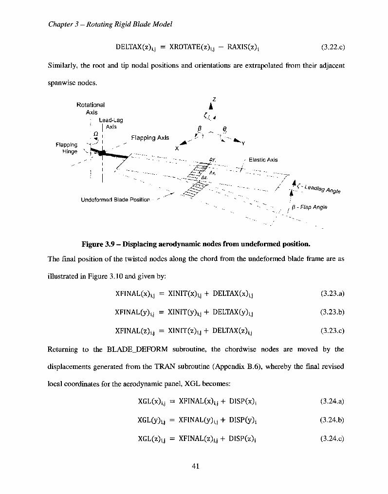
DELTAX(z)i;j = XROTATE(z\j - RAXIS(z)t (3.22.c)
Similarly, the root and tip nodal positions and orientations are extrapolated from their adjacent
spanwise nodes.
Rotational
Flapping Hinge
Axis : Lead-Lag ] 1 Axis
:5l rxli •-' v^f-, _ . ,' 1 l---7
'
Flapping
s .
• . .
Undeformed Blade Position -
Axis
-—-
--
X
---—..
"~ ~-.--*i
»-~- ...<<:
Z A
< ( . <
A ^ ^ T
&•
j£r—>f Ax,
~^AZ-
•^$?~~L -
~F~ • •
e, x ^
—---
• Ak. . Y
r-
-i-_.
- — •
-
Elastic Axis
*""""- -'? /
- •- r
--.. " -.
4 r ,V
C:Lea^9Ang/e
- Flap Angle
Figure 3.9 - Displacing aerodynamic nodes from undeformed position.
The final position of the twisted nodes along the chord from the undeformed blade frame are as
illustrated in Figure 3.10 and given by:
XFINAL(x)y = XINIT(x)jj + DELTAX(x)jj (3.23.a)
XFINAL(y)jj = XINIT(y)y + DELTAX(y)y (3.23.b)
XFINAL(z)i.j = XINIT(z)y + DELTAX(z)jj (3.23.c)
Returning to the BLADE_DEFORM subroutine, the chordwise nodes are moved by the
displacements generated from the TRAN subroutine (Appendix B.6), whereby the final revised
local coordinates for the aerodynamic panel, XGL becomes:
XGL(x)ij = XFINAL(x)jj + DISP(x)j (3.24.a)
XGL(y)ij = XFINALGOij + DISP(y)i (3.24.b)
XGL(z)y = XFINAL(z)i;j + DISP(z)j (3.24.c)
41
Chapter 3 - Rotating Rigid Blade Model
&je*G Spanwl&e Lines x17 Aero Chordwise Lines x9
Ic ls l Intersects 1 t>j
Noam «145
<--^-LeadlagAngh
Node S163 I = 17 / = S )
j8 - Flap Angle
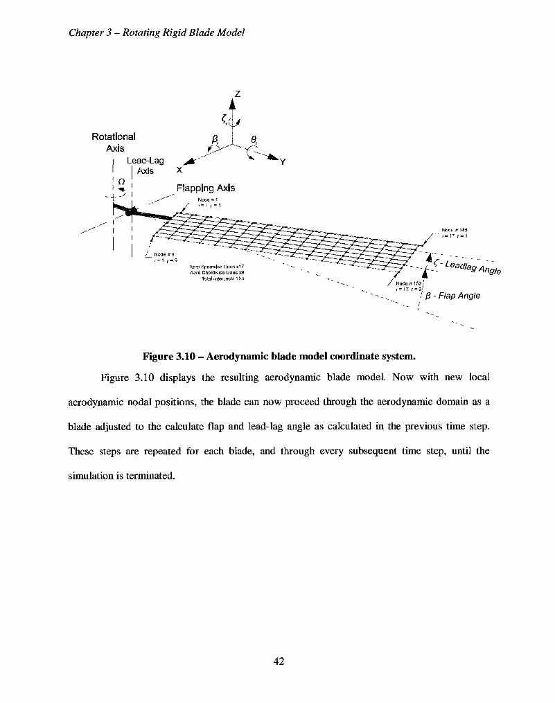
Figure 3.10 - Aerodynamic blade model coordinate system.
Figure 3.10 displays the resulting aerodynamic blade model. Now with new local
aerodynamic nodal positions, the blade can now proceed through the aerodynamic domain as a
blade adjusted to the calculate flap and lead-lag angle as calculated in the previous time step.
These steps are repeated for each blade, and through every subsequent time step, until the
simulation is terminated.
42
Chapter 4 - CH-47C Rotor Blade Flapping Motion Analysis
Chapter 4 CH-47C Rotor Blade Flapping Motion Analysis
In 1972, an experiment on blade motion characteristics was conducted. The results of the
experiment were presented in Harris' paper entitled "Articulated Rotor Blade Flapping Motion at
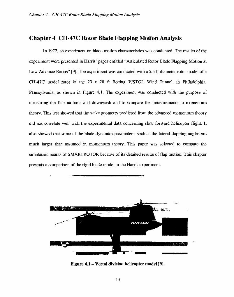
Low Advance Ratios" [9]. The experiment was conducted with a 5.5 ft diameter rotor model of a
CH-47C model rotor in the 20 x 20 ft Boeing V/STOL Wind Tunnel, in Philadelphia,
Pennsylvania, as shown in Figure 4.1. The experiment was conducted with the purpose of
measuring the flap motions and downwash and to compare the measurements to momentum
theory. This test showed that the wake geometry predicted from the advanced momentum theory
did not correlate well with the experimental data concerning slow forward helicopter flight. It
also showed that some of the blade dynamics parameters, such as the lateral flapping angles are
much larger than assumed in momentum theory. This paper was selected to compare the
simulation results of SMARTROTOR because of its detailed results of flap motion. This chapter
presents a comparison of the rigid blade model to the Harris experiment.
Figure 4.1 - Vertol division helicopter model [9].
43
Chapter 4 - CH-47C Rotor Blade Flapping Motion Analysis
4.1 Harris Articulated Blade Flapping Motion Overview
Harris [9] conducted three experiments to measure the flapping motions due to the
influence of advance ratios, collective pitch, and shaft tilt. Simulations with SMARTROTOR's
rigid blade model reproduced Harris' three experiments. The original experiment removed the
forward rotor blades of the tandem helicopter as a means to isolate the aft rotor blades to allow
for clean undisturbed oncoming air stream. The data collected was taken through increasing
incoming velocities or advance ratios of 0 to 0.24. The results showed that the maximum
amplitude of flapping motion of 3.4° occurred at 0.08 advance ratio. The blade motion was
recorded with a Rotary Variable Displacement Transformer. The rotor rotated at a tip speed of
137.16 m/s or a rotational speed of 164.8 rad/s (26.2 Hz). The rotor geometry is described in
Table 4.1 below:
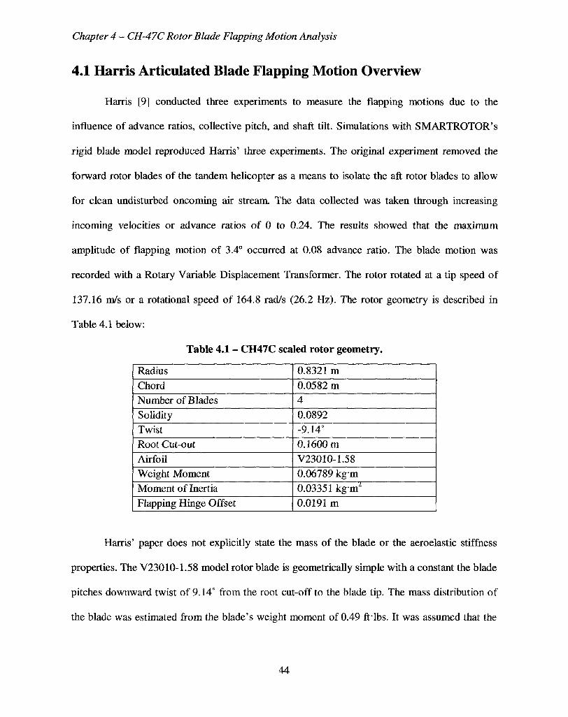
Table 4.1 - CH47C scaled rotor geometry.
Radius Chord Number of Blades Solidity Twist Root Cut-out Airfoil Weight Moment Moment of Inertia Flapping Hinge Offset
0.8321 m 0.0582 m 4 0.0892 -9.14° 0.1600 m V23010-1.58 0.06789 kgm 0.03351 kg-m2
0.0191 m
Harris' paper does not explicitly state the mass of the blade or the aeroelastic stiffness
properties. The V23010-1.58 model rotor blade is geometrically simple with a constant the blade
pitches downward twist of 9.14° from the root cut-off to the blade tip. The mass distribution of
the blade was estimated from the blade's weight moment of 0.49 fHbs. It was assumed that the
44
Chapter 4 - CH-47C Rotor Blade Flapping Motion Analysis
blade has a near-uniform mass distribution form the root cut to the tip, as there is no significant
variance in blade geometry. For a beam with a fixed end, the bending moment is:
A f = = £ (4.1)
and the blade length L from hinge point to blade tip is 0.813 m, so the distributed mass m is
estimated to be 0.205 kg/m.
To comply with the equations of motion (Eqs. 3.7 and 3.8), it is assumed that the blade is
rigid. In reality the blade will experience flexing, but with a hinged blade the magnitude of the
flexing should be small relative to the amplitudes of the flap and lead-lag motion.
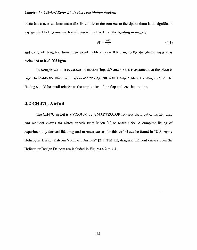
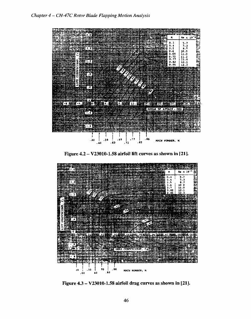
4.2 CH47C Airfoil
The CH47C airfoil is a V2301O-1.58. SMARTROTOR requires the input of the lift, drag
and moment curves for airfoil speeds from Mach 0.0 to Mach 0.95. A complete listing of
experimentally derived lift, drag and moment curves for this airfoil can be found in "U.S. Army
Helicopter Design Datcom Volume 1 Airfoils" [21]. The lift, drag and moment curves from the
Helicopter Design Datcom are included in Figures 4.2 to 4.4.
45
Chapter 4 - CH-47C Rotor Blade Flapping Motion Analysis
MACS tfUHi£ft. K
Figure 4.2 - V23010-1.58 airfoil Uft curves as shown in [21].
Figure 4.3 - V23010-1.58 airfoil drag curves as shown in [21].
46
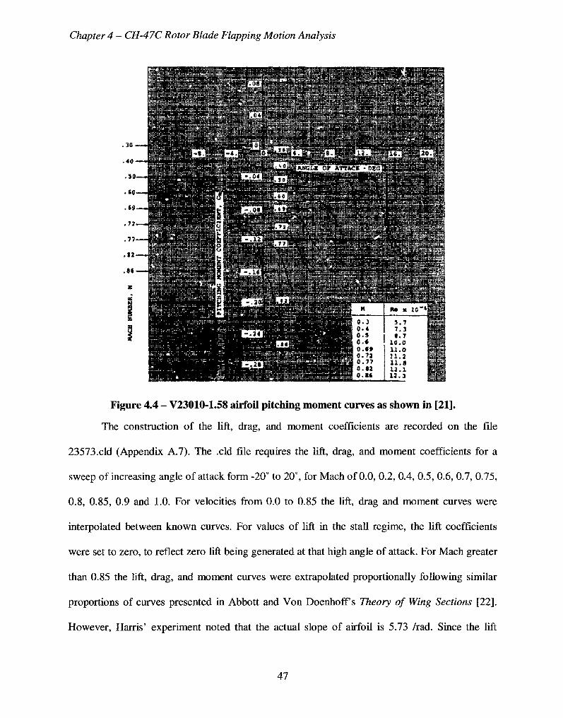
Chapter 4 - CH-47C Rotor Blade Flapping Motion Analysis
Figure 4.4 - V23010-1.58 airfoil pitching moment curves as shown in [21].
The construction of the lift, drag, and moment coefficients are recorded on the file
23573.cld (Appendix A.7). The .eld file requires the lift, drag, and moment coefficients for a
sweep of increasing angle of attack form -20° to 20°, for Mach of 0.0, 0.2, 0.4, 0.5, 0.6, 0.7, 0.75,
0.8, 0.85, 0.9 and 1.0. For velocities from 0.0 to 0.85 the lift, drag and moment curves were
interpolated between known curves. For values of lift in the stall regime, the lift coefficients
were set to zero, to reflect zero lift being generated at that high angle of attack. For Mach greater
than 0.85 the lift, drag, and moment curves were extrapolated proportionally following similar
proportions of curves presented in Abbott and Von Doenhoff s Theory of Wing Sections [22].
However, Harris' experiment noted that the actual slope of airfoil is 5.73 /rad. Since the lift
47
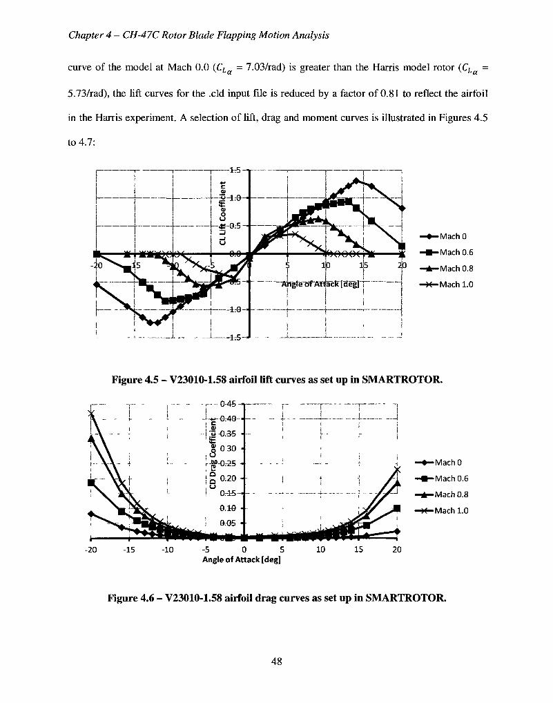
Chapter 4 - CH-47C Rotor Blade Flapping Motion Analysis
curve of the model at Mach 0.0 (CLa = 7.03/rad) is greater than the Harris model rotor (CL =
5.73/rad), the lift curves for the .eld input file is reduced by a factor of 0.81 to reflect the airfoil
in the Harris experiment. A selection of lift, drag and moment curves is illustrated in Figures 4.5
to 4.7:
•MachO
•Mach 0.6
•Mach 0.8
•Mach 1.0
Figure 4.5 - V23010-1.58 airfoil lift curves as set up in SMARTROTOR.
0-45
-5 0 5 Angle of Attack [deg]
•MachO
•Mach 0.6
•Mach 0.8
•Mach 1.0
Figure 4.6 - V23010-1.58 airfoil drag curves as set up in SMARTROTOR.
48
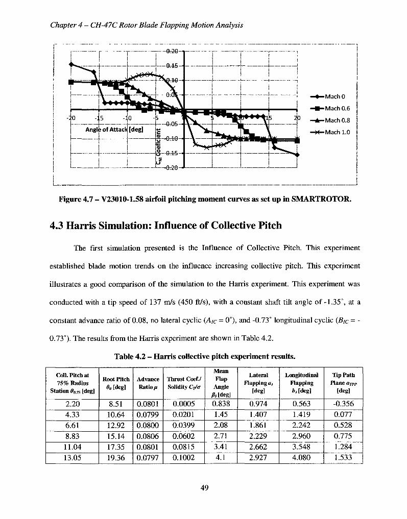
Chapter 4 - CH-47C Rotor Blade Flapping Motion Analysis
Figure 4.7 - V23010-1.58 airfoil pitching moment curves as set up in SMARTROTOR.
4.3 Harris Simulation: Influence of Collective Pitch
The first simulation presented is the Influence of Collective Pitch. This experiment
established blade motion trends on the influence increasing collective pitch. This experiment
illustrates a good comparison of the simulation to the Harris experiment. This experiment was
conducted with a tip speed of 137 m/s (450 ft/s), with a constant shaft tilt angle of -1.35°, at a
constant advance ratio of 0.08, no lateral cyclic (AJC - 0°), and -0.73° longitudinal cyclic (Bic = -
0.73°). The results from the Harris experiment are shown in Table 4.2.
Table 4.2 - Harris collective pitch experiment results.
Coll. Pitch at 75% Radius
Station 0Oj5 [deg]
2.20 4.33 6.61 8.83 11.04 13.05
Root Pitch 0o [deg]
8.51 10.64 12.92 15.14 17.35 19.36
Advance Ratio/*
0.0801 0.0799 0.0800 0.0806 0.0801 0.0797
Thrust CoefJ Solidity Cj/a
0.0005 0.0201 0.0399 0.0602 0.0815 0.1002
Mean Flap
Angle Mdeg]
0.838 1.45 2.08 2.71 3.41 4.1
Lateral Flapping a?
[deg]
0.974 1.407 1.861 2.229 2.662 2.927
Longitudinal Flapping Mdeg]
0.563 1.419 2.242 2.960 3.548 4.080
Tip Path Plane aTpp
[deg]
-0.356 0.077 0.528 0.775 1.284 1.533
49
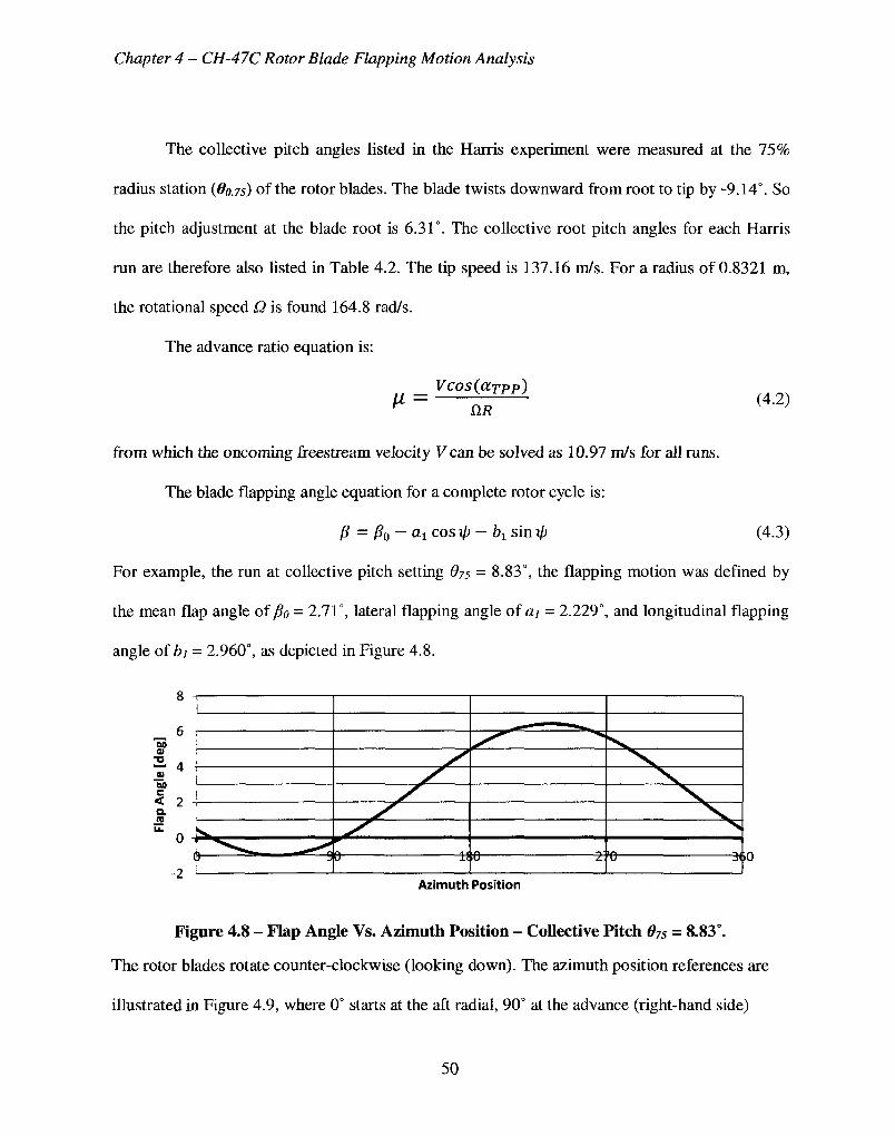
Chapter 4 - CH-47C Rotor Blade Flapping Motion Analysis
The collective pitch angles listed in the Harris experiment were measured at the 75%
radius station {do.75) of the rotor blades. The blade twists downward from root to tip by -9.14°. So
the pitch adjustment at the blade root is 6.31°. The collective root pitch angles for each Harris
run are therefore also listed in Table 4.2. The tip speed is 137.16 m/s. For a radius of 0.8321 m,
the rotational speed Q is found 164.8 rad/s.
The advance ratio equation is:
VCOS(CCTPP) l* = Q.R
(4.2)
from which the oncoming freestream velocity V can be solved as 10.97 m/s for all runs.
The blade flapping angle equation for a complete rotor cycle is:
/? = /?0 — ax cos i/> — bx sin ip (4.3)
For example, the run at collective pitch setting 675 = 8.83°, the flapping motion was defined by
the mean flap angle of /?o = 2.71°, lateral flapping angle of ai = 2.229°, and longitudinal flapping
angle of bi = 2.960°, as depicted in Figure 4.8.
3( i0
Azimuth Position
Figure 4.8 - Flap Angle Vs. Azimuth Position - Collective Pitch 075 = 8.83°.
The rotor blades rotate counter-clockwise (looking down). The azimuth position references are
illustrated in Figure 4.9, where 0° starts at the aft radial, 90° at the advance (right-hand side)
50
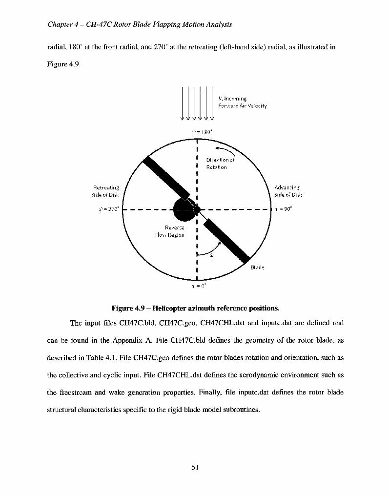
Chapter 4 - CH-47C Rotor Blade Flapping Motion Analysis
radial, 180° at the front radial, and 270° at the retreating (left-hand side) radial, as illustrated in
Figure 4.9.
v, Incoming Forward Air Velocity
Retreating Side of Disk
a'' = 270'
Advancing Side of Disk
.']• = 90°
.•;• = 0'
Figure 4.9 - Helicopter azimuth reference positions.
The input files CH47C.bld, CH47C.geo, CH47CHL.dat and inputc.dat are defined and
can be found in the Appendix A. File CH47C.bld defines the geometry of the rotor blade, as
described in Table 4.1. File CH47C.geo defines the rotor blades rotation and orientation, such as
the collective and cyclic input. File CH47CHL.dat defines the aerodynamic environment such as
the freestream and wake generation properties. Finally, file inputc.dat defines the rotor blade
structural characteristics specific to the rigid blade model subroutines.
51
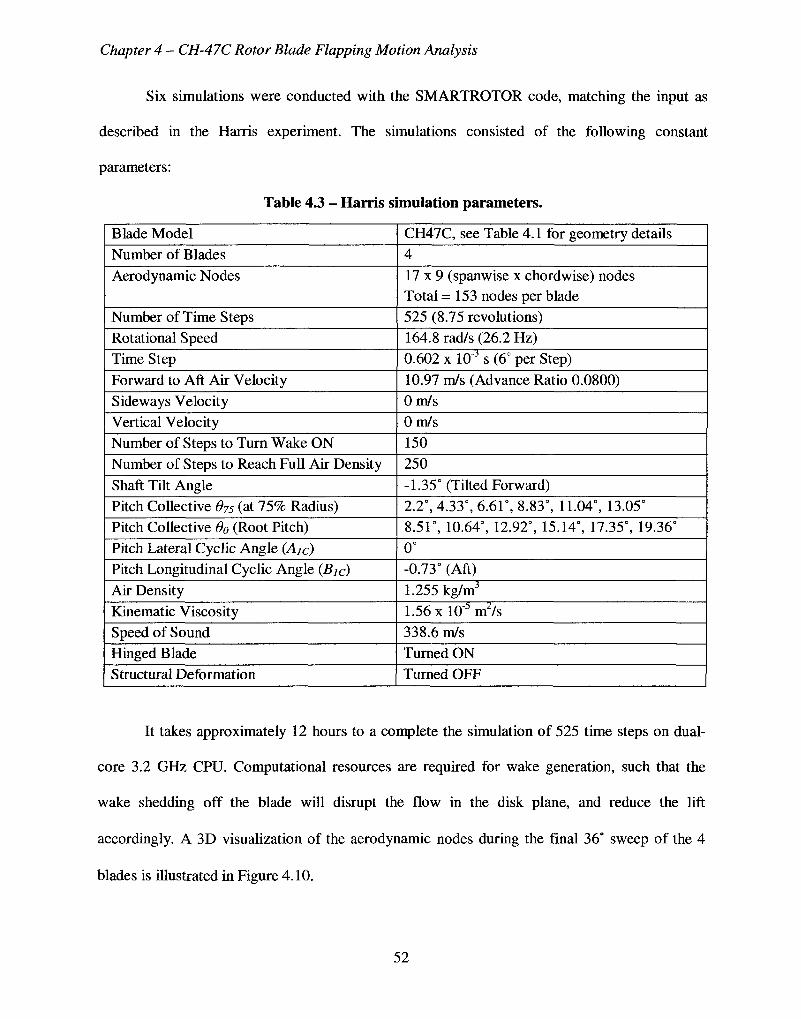
Chapter 4 - CH-47C Rotor Blade Flapping Motion Analysis
Six simulations were conducted with the SMARTROTOR code, matching the input as
described in the Harris experiment. The simulations consisted of the following constant
parameters:
Table 4.3 - Harris simulation parameters.
Blade Model
Number of Blades
Aerodynamic Nodes
Number of Time Steps
Rotational Speed
Time Step
Forward to Aft Air Velocity
Sideways Velocity
Vertical Velocity
Number of Steps to Turn Wake ON
Number of Steps to Reach Full Air Density
Shaft Tilt Angle
Pitch Collective 6>75 (at 75% Radius)
Pitch Collective 60 (Root Pitch)
Pitch Lateral Cyclic Angle (A1C)
Pitch Longitudinal Cyclic Angle (B1C)
Air Density
Kinematic Viscosity
Speed of Sound
Hinged Blade
Structural Deformation
CH47C, see Table 4.1 for geometry details
4
1 7 x 9 (spanwise x chordwise) nodes
Total =153 nodes per blade
525 (8.75 revolutions)
164.8 rad/s (26.2 Hz)
0.602 x 10"3 s (6° per Step)
10.97 m/s (Advance Ratio 0.0800)
Om/s
Om/s
150
250
-1.35° (Tilted Forward)
2.2°, 4.33°, 6.61°, 8.83°, 11.04°, 13.05°
8.51°, 10.64°, 12.92°, 15.14°, 17.35°, 19.36°
0°
-0.73° (Aft)
1.255 kg/m"
1.56 x lO"3 m7/s
338.6 m/s
Turned ON
Turned OFF
It takes approximately 12 hours to a complete the simulation of 525 time steps on dual-
core 3.2 GHz CPU. Computational resources are required for wake generation, such that the
wake shedding off the blade will disrupt the flow in the disk plane, and reduce the lift
accordingly. A 3D visualization of the aerodynamic nodes during the final 36° sweep of the 4
blades is illustrated in Figure 4.10.
52
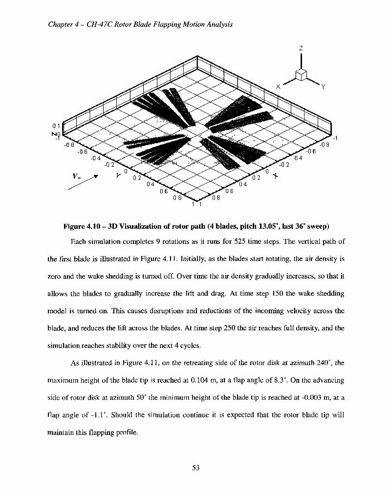
Chapter 4 - CH-47C Rotor Blade Flapping Motion Analysis
Figure 4.10 - 3D Visualization of rotor path (4 blades, pitch 13.05°, last 36° sweep)
Each simulation completes 9 rotations as it runs for 525 time steps. The vertical path of
the first blade is illustrated in Figure 4.11. Initially, as the blades start rotating, the air density is
zero and the wake shedding is turned off. Over time the air density gradually increases, so that it
allows the blades to gradually increase the lift and drag. At time step 150 the wake shedding
model is turned on. This causes disruptions and reductions of the incoming velocity across the
blade, and reduces the lift across the blades. At time step 250 the air reaches full density, and the
simulation reaches stability over the next 4 cycles.
As illustrated in Figure 4.11, on the retreating side of the rotor disk at azimuth 240°, the
maximum height of the blade tip is reached at 0.104 m, at a flap angle of 8.3°. On the advancing
side of rotor disk at azimuth 50° the minimum height of the blade tip is reached at -0.003 m, at a
flap angle of -1.1°. Should the simulation continue it is expected that the rotor blade tip will
maintain this flapping profile.
53
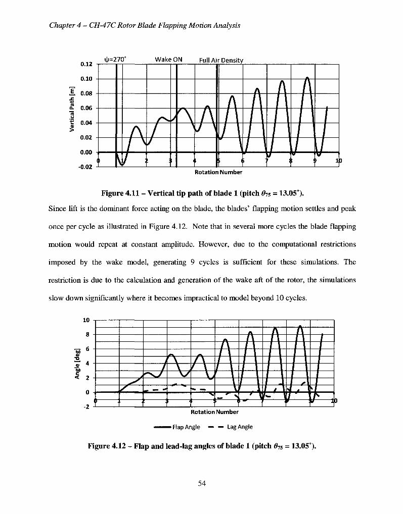
Chapter 4 - CH-47C Rotor Blade Flapping Motion Analysis
0.12
0.10
J . 0.08
S. 0.06
il)=270° Wake ON Full Air Density
01 >
0.04
0.02
0.00
-0.02 0
t
__zy _. : :i
. A
\A >y \
4
A / \
\
\ ; i
A
A /
/
A A I
i f : 1 ! 1 10
Rotation Number
Figure 4.11 - Vertical tip path of blade 1 (pitch 9-JS = 13.05°).
Since lift is the dominant force acting on the blade, the blades' flapping motion settles and peak
once per cycle as illustrated in Figure 4.12. Note that in several more cycles the blade flapping
motion would repeat at constant amplitude. However, due to the computational restrictions
imposed by the wake model, generating 9 cycles is sufficient for these simulations. The
restriction is due to the calculation and generation of the wake aft of the rotor, the simulations
slow down significantly where it becomes impractical to model beyond 10 cycles.
10
DO 01
< 2
II :
•
< '
« . _ »
1 !
I t \ l*~ \
1 f\ *m. » \
• b «*• i w a / J b Rotation Number
•Flap Angle — — Lag Angle
Figure 4.12 - Flap and lead-lag angles of blade 1 (pitch 07S = 13.05°).
54
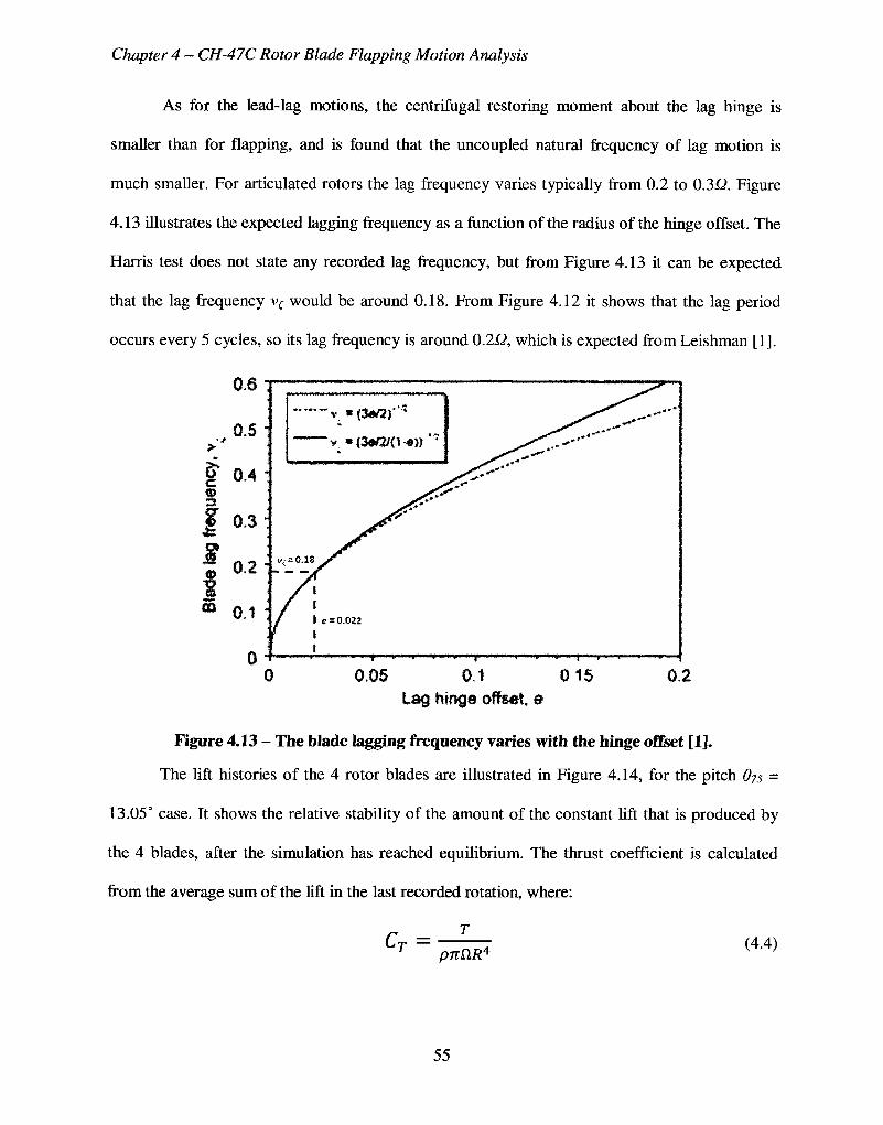
Chapter 4 - CH-47C Rotor Blade Flapping Motion Analysis
As for the lead-lag motions, the centrifugal restoring moment about the lag hinge is
smaller than for flapping, and is found that the uncoupled natural frequency of lag motion is
much smaller. For articulated rotors the lag frequency varies typically from 0.2 to 0.342. Figure
4.13 illustrates the expected lagging frequency as a function of the radius of the hinge offset. The
Harris test does not state any recorded lag frequency, but from Figure 4.13 it can be expected
that the lag frequency vf would be around 0.18. From Figure 4.12 it shows that the lag period
occurs every 5 cycles, so its lag frequency is around 0.2,0, which is expected from Leishman [1].
0.6 l
0.5
f 0.4
f 0.3 '
CO
0.2"
0.1:
v,-s0.1S
e = 0.022
wf^mmm^mmmx^mfmmt-mmm^m !' " •
0,05 0.1 015 Lag hinge offset, &
0.2
Figure 4.13 - The blade lagging frequency varies with the hinge offset [1].
The lift histories of the 4 rotor blades are illustrated in Figure 4.14, for the pitch 675 =
13.05° case. It shows the relative stability of the amount of the constant lift that is produced by
the 4 blades, after the simulation has reached equilibrium. The thrust coefficient is calculated
from the average sum of the lift in the last recorded rotation, where:
T pnClR4 (4.4)
55
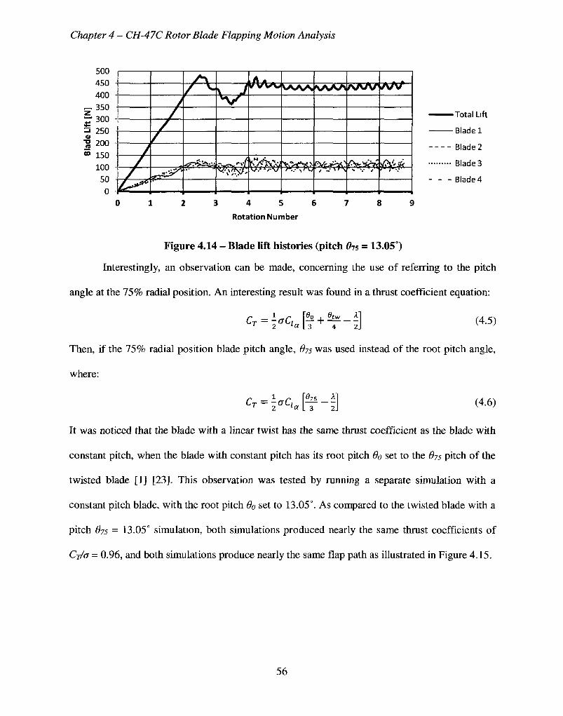
Chapter 4 - CH-47C Rotor Blade Flapping Motion Analysis
- Total Lift
Blade 1
Blade 2
Blade 3
Blade 4
0 1 2 3 4 5 6 7 8 9
Rotation Number
Figure 4.14 - Blade lift histories (pitch d7S = 13.05°)
Interestingly, an observation can be made, concerning the use of referring to the pitch
angle at the 75% radial position. An interesting result was found in a thrust coefficient equation:
^- i '< i 1 ,&+ s f - j | («)
Then, if the 75% radial position blade pitch angle, 675 was used instead of the root pitch angle,
where:
It was noticed that the blade with a linear twist has the same thrust coefficient as the blade with
constant pitch, when the blade with constant pitch has its root pitch do set to the 875 pitch of the
twisted blade [1] [23]. This observation was tested by running a separate simulation with a
constant pitch blade, with the root pitch 60 set to 13.05°. As compared to the twisted blade with a
pitch 675 = 13.05° simulation, both simulations produced nearly the same thrust coefficients of
Crh = 0.96, and both simulations produce nearly the same flap path as illustrated in Figure 4.15.
56
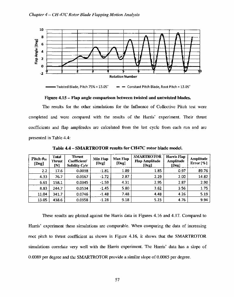
Chapter 4 - CH-47C Rotor Blade Flapping Motion Analysis
bo CD
CD
BO
c < Q. (0
10
8
6
4
2
0
-2
\ * j
o :: :i n :. (> f y i Rotation Number
Twisted Blade, Pitch 75% = 13.05° — — Constant Pitch Blade, Root Pitch = 13.05"
Figure 4.15 - Flap angle comparison between twisted and untwisted blades.
The results for the other simulations for the Influence of Collective Pitch test were
completed and were compared with the results of the Harris' experiment. Their thrust
coefficients and flap amplitudes are calculated from the last cycle from each run and are
presented in Table 4.4:
Table 4.4 - SMARTROTOR results for CH47C rotor blade model.
Pitch 07s [Deg]
2.2
4.33
6.61
8.83
11.04
13.05
Total Thrust
[N] 17.6
76.7
158.1
244.7
341.7
438.6
Thrust Coefficient/
Solidity Cj/tr
0.0038
0.0167
0.0345
0.0534
0.0746
0.0958
Min Flap [Deg]
-1.81
-1.72
-1.59
-1.45
-1.48
-1.28
Max Flap [Deg]
1.89
2.87
4.31
5.80
7.48
9.18
SMARTROTOR Flap Amplitude
[Deg]
1.85
2.29
2.95
3.62
4.48
5.23
Harris Flap Amplitude
[Deg] 0.97
2.00
2.87
3.56
4.26
4.76
Amplitude Error [%]
89.76
14.82
2.90
1.75
5.19
9.94
These results are plotted against the Harris data in Figures 4.16 and 4.17. Compared to
Harris' experiment these simulations are comparable. When comparing the data of increasing
root pitch to thrust coefficient as shown in Figure 4.16, it shows that the SMARTROTOR
simulations correlate very well with the Harris experiment. The Harris' data has a slope of
0.0089 per degree and the SMARTROTOR provide a similar slope of 0.0085 per degree.
57
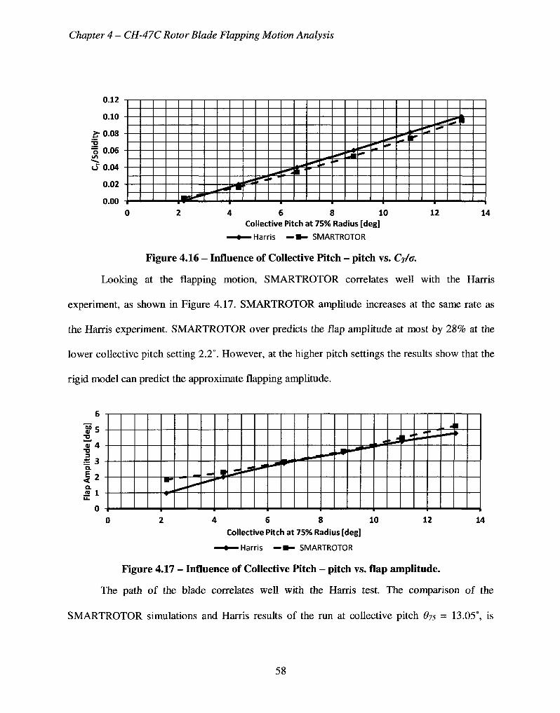
Chapter 4 - CH-47C Rotor Blade Flapping Motion Analysis
0.12 -|
"D
o u.uo -
0.00
mi TS_ • «" *•
^ 5 ^ '
4 6 8 10 Collective Pitch at 75% Radius [deg]
> Harris — • - SMARTROTOR
12 14
Figure 4.16 - Influence of Collective Pitch - pitch vs. Cj/a.
Looking at the flapping motion, SMARTROTOR correlates well with the Harris
experiment, as shown in Figure 4.17. SMARTROTOR amplitude increases at the same rate as
the Harris experiment. SMARTROTOR over predicts the flap amplitude at most by 28% at the
lower collective pitch setting 2.2°. However, at the higher pitch settings the results show that the
rigid model can predict the approximate flapping amplitude.
ai 4 •o 3 £ 3 Q. | 2 Q.
JS 1
0 4 0
' ' ' i ' ' ' i ' ' ' i ' ' ' i ' ' ' i ' '
4 6 8 10 Collective Pitch at 75% Radius [deg]
> Harris — • - SMARTROTOR
12 14
Figure 4.17 - Influence of Collective Pitch - pitch vs. flap amplitude.
The path of the blade correlates well with the Harris test. The comparison of the
SMARTROTOR simulations and Harris results of the run at collective pitch 675 = 13.05°, is
58
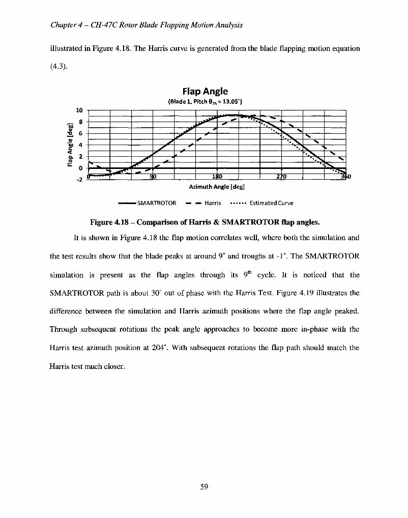
Chapter 4 - CH-47C Rotor Blade Flapping Motion Analysis
illustrated in Figure 4.18. The Harris curve is generated from the blade flapping motion equation
(4.3).
Flap Angle (Blade 1, Pitch 675= 13.05°)
^
- - • £
y *
0
^
** *
180
"*?> ^ • • > V
«.N ^
w X • - \ w
• ^ k
2'0
N N
"V ' '
*.
s. V
"••S* 31
Azimuth Angle [deg]
SMARTROTOR — — Harris Estimated Curve
Figure 4.18 - Comparison of Harris & SMARTROTOR flap angles.
It is shown in Figure 4.18 the flap motion correlates well, where both the simulation and
the test results show that the blade peaks at around 9° and troughs at -1°. The SMARTROTOR
simulation is present as the flap angles through its 9th cycle. It is noticed that the
SMARTROTOR path is about 30° out of phase with the Harris Test. Figure 4.19 illustrates the
difference between the simulation and Harris azimuth positions where the flap angle peaked.
Through subsequent rotations the peak angle approaches to become more in-phase with the
Harris test azimuth position at 204°. With subsequent rotations the flap path should match the
Harris test much closer.
59
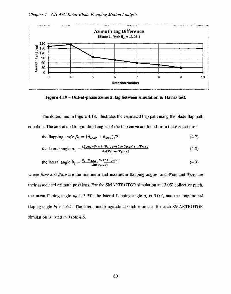
Chapter 4 - CH-47C Rotor Blade Flapping Motion Analysis
BO
a> BO <0
180 150
E
3
120 f 90
60
30
Azimuth Lag Difference (Blade 1, Pitch 875= 13.05°)
~ -O
6 7
Rotation Number
10
Figure 4.19 - Out-of-phase azimuth lag between simulation & Harris test.
The dotted line in Figure 4.18, illustrates the estimated flap path using the blade flap path
equation. The lateral and longitudinal angles of the flap curve are found from these equations:
the flapping angle /?0 = {PMAX + / W ) / 2 (4-7)
(PMiN-Msin "VMAXHPO-PMAX) sin V>MAX the lateral angle ax =
the lateral angle bt
smQVMIN-'VMAx)
PO-PMAX-^I COS^MAX
(4.8)
(4.9) sinOFjvMx)
where 0MIN and PMAX are the minimum and maximum flapping angles, and WMIN and WMAX are
their associated azimuth positions. For the SMARTROTOR simulation at 13.05° collective pitch,
the mean flaping angle fi0 is 3.95°, the lateral flapping angle at is 5.00°, and the longitudinal
flaping angle bi is 1.62°. The lateral and longitudinal pitch estimates for each SMARTROTOR
simulation is listed in Table 4.5.
60
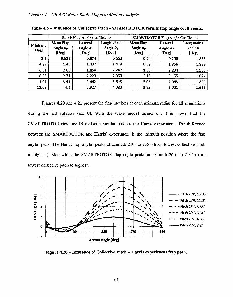
Chapter 4 - CH-47C Rotor Blade Flapping Motion Analysis
Table 4.5 - Influence of Collective Pitch - SMARTROTOR results flap angle coefficients.
Pitch 075
[Deg]
2.2
4.33
6.61
8.83
11.04
13.05
Harris Flap Angle Coefficients Mean Flap Angle Po
[Deg]
0.838
1.45
2.08
2.71
3.41
4.1
Lateral Angle ai
[Deg] 0.974
1.407
1.864
2.229
2.662
2.927
Longitudinal Angle bj
[Deg]
0.563
1.419
2.242
2.960
3.548
4.080
SMARTROTOR Flap Angle Coefficients Mean Flap Angle Po
[Deg]
0.04
0.58
1.36
2.18
3.06
3.95
Lateral Angle ai
[Deg]
0.258
1.356
2.204
3.155
4.063
5.001
Longitudinal Angle bj
[Deg]
1.833
1.866
1.985
1.822
1.809
1.625
Figures 4.20 and 4.21 present the flap motions at each azimuth radial for all simulations
during the last rotation (no. 9). With the wake model turned on, it is shown that the
SMARTROTOR rigid model makes a similar path as the Harris experiment. The difference
between the SMARTROTOR and Harris' experiment is the azimuth position where the flap
angles peak. The Harris flap angles peaks at azimuth 210° to 235° (from lowest collective pitch
to highest). Meanwhile the SMARTROTOR flap angle peaks at azimuth 260° to 210° (from
lowest collective pitch to highest).
J .U •*
<u c < Q .
t i
ll " L̂ •.
i^flJflff^l^H T
> • /
A* &£
Azi
/4
/ /
' , \
> '
1'
mthAi
/ *
' '
^
tn
igle [c
•
. • "
eg]
•
>>
^
" ^
•v
•h
\N • v *
• " - .
'11
L
. . A s \ \ N > \
•>t
-Pitch75%, 13.05
— — Pitch 75%, 11.04
— • - Pitch 75%, 8.83°
- - - Pitch 75%, 6.61°
Pitch 75%, 4.33°
— — Pitch 75%, 2.2°
in
Figure 4.20 - Influence of Collective Pitch - Harris experiment flap path.
61
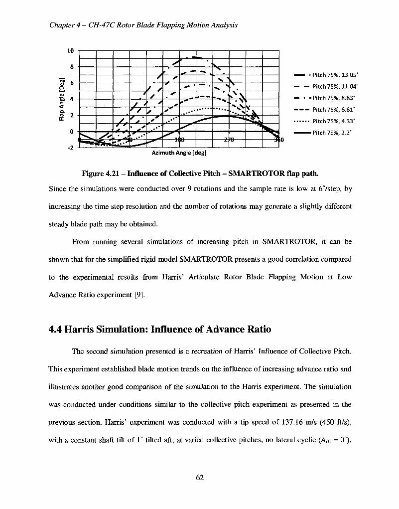
Chapter 4 - CH-47C Rotor Blade Flapping Motion Analysis
— • Pitch 75%, 13.05°
Pitch 75%, 11.04°
— • - Pitch 75%, 8.83°
- - - Pitch 75%, 6.61°
Pitch 75%, 4.33°
Pitch 75%, 2.2° iO
Azimuth Angle [deg]
Figure 4.21 - Influence of Collective Pitch - SMARTROTOR flap path.
Since the simulations were conducted over 9 rotations and the sample rate is low at 67step, by
increasing the time step resolution and the number of rotations may generate a slightly different
steady blade path may be obtained.
From running several simulations of increasing pitch in SMARTROTOR, it can be
shown that for the simplified rigid model SMARTROTOR presents a good correlation compared
to the experimental results from Harris' Articulate Rotor Blade Flapping Motion at Low
Advance Ratio experiment [9].
4.4 Harris Simulation: Influence of Advance Ratio
The second simulation presented is a recreation of Harris' Influence of Collective Pitch.
This experiment established blade motion trends on the influence of increasing advance ratio and
illustrates another good comparison of the simulation to the Harris experiment. The simulation
was conducted under conditions similar to the collective pitch experiment as presented in the
previous section. Harris' experiment was conducted with a tip speed of 137.16 m/s (450 ft/s),
with a constant shaft tilt of 1° tilted aft, at varied collective pitches, no lateral cyclic (AIC = 0°),
J . U
bo
a tu DO c < Q.
_re
6
4
2
^ ^^f*^BJ
/ , r S
s' t"
• * / *
• • *' '
' / * • • •
, - lr ••• •?..*> If-
• t * *
" , . -
r
*
'
. . .-•• '
.*• ""
- * > •
^ —
, - • •
' s_ X
N \ m*
» ——
. . • • • •
- > .
, \ \
"̂̂ ••.. •* - *
1
It *SA
Jl
62
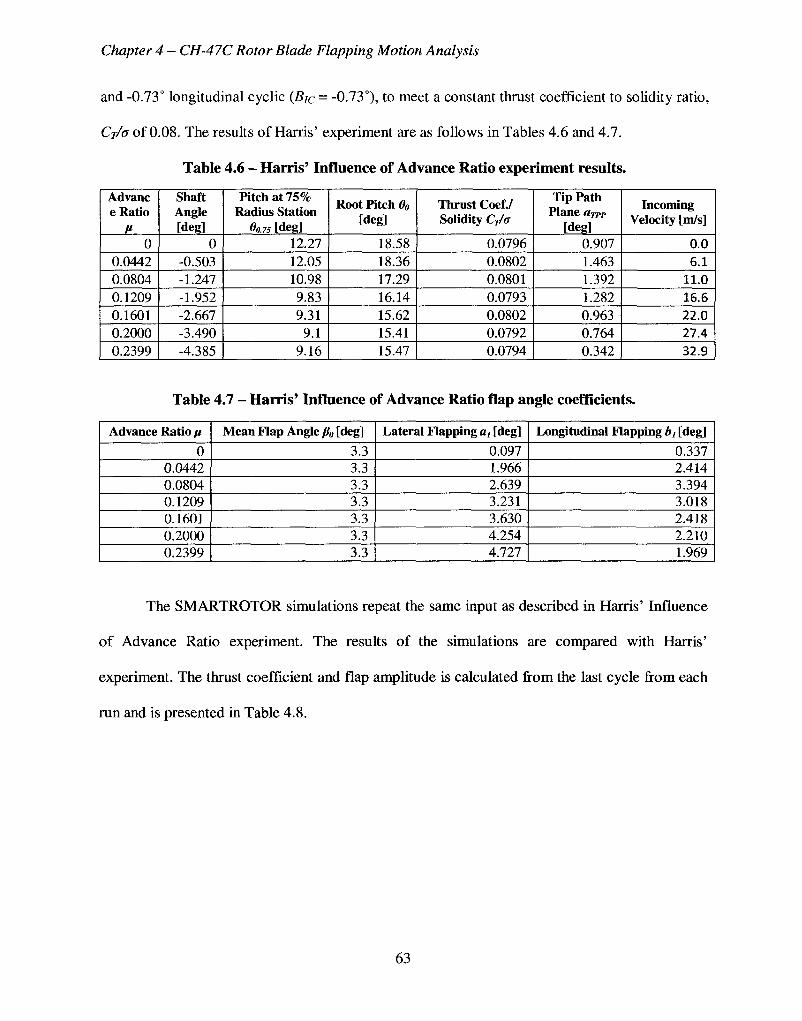
Chapter 4 - CH-47C Rotor Blade Flapping Motion Analysis
and -0.73° longitudinal cyclic {BjC = -0.73°), to meet a constant thrust coefficient to solidity ratio,
Ci/cr of 0.08. The results of Harris' experiment are as follows in Tables 4.6 and 4.7.
Table 4.6 - Harris' Influence of Advance Ratio experiment results.
Advanc e Ratio
0 0.0442 0.0804 0.1209 0.1601 0.2000 0.2399
Shaft Angle [deg]
0 -0.503 -1.247 -1.952 -2.667 -3.490 -4.385
Pitch at 75% Radius Station
OOJS [deg]
12.27 12.05 10.98 9.83 9.31
9.1 9.16
Root Pitch 0O
[deg]
18.58 18.36 17.29 16.14 15.62 15.41 15.47
Thrust Coef./ Solidity Cjlo
0.0796 0.0802 0.0801 0.0793 0.0802 0.0792 0.0794
Tip Path Plane aTPP
[deg] 0.907 1.463 1.392 1.282 0.963 0.764 0.342
Incoming Velocity [m/s]
0.0 6.1
11.0 16.6 22.0 27.4 32.9
Table 4.7 - Harris' Influence of Advance Ratio flap angle coefficients.
Advance Ratio /i
0 0.0442 0.0804 0.1209 0.1601 0.2000 0.2399
Mean Flap Angle /?»[deg]
3.3 3.3 3.3 3.3 3.3 3.3 3.3
Lateral Flapping a, [deg]
0.097 1.966 2.639 3.231 3.630 4.254 4.727
Longitudinal Flapping b, [deg]
0.337 2.414 3.394 3.018 2.418 2.210 1.969
The SMARTROTOR simulations repeat the same input as described in Harris' Influence
of Advance Ratio experiment. The results of the simulations are compared with Harris'
experiment. The thrust coefficient and flap amplitude is calculated from the last cycle from each
run and is presented in Table 4.8.
63
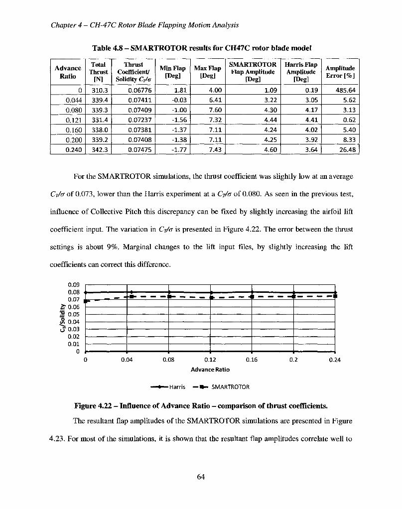
Chapter 4 - CH-47C Rotor Blade Flapping Motion Analysis
Table 4.8 - SMARTROTOR results for CH47C rotor blade model
Advance Ratio
0
0.044
0.080
0.121
0.160
0.200
0.240
Total Thrust
[N]
310.3
339.4
339.3
331.4
338.0
339.2
342.3
Thrust Coefficient/ Solidity Cj/a
0.06776
0.07411
0.07409
0.07237
0.07381
0.07408
0.07475
Min Flap [Deg]
1.81
-0.03
-1.00
-1.56
-1.37
-1.38
-1.77
Max Flap [Deg]
4.00
6.41
7.60
7.32
7.11
7.11
7.43
SMARTROTOR Flap Amplitude
[Deg]
1.09
3.22
4.30
4.44
4.24
4.25
4.60
Harris Flap Amplitude
[Deg]
0.19
3.05
4.17
4.41
4.02
3.92
3.64
Amplitude Error [%]
485.64
5.62
3.13
0.62
5.40
8.33
26.48
For the SMARTROTOR simulations, the thrust coefficient was slightly low at an average
Ci/o of 0.073, lower than the Harris experiment at a C-j/a of 0.080. As seen in the previous test,
influence of Collective Pitch this discrepancy can be fixed by slightly increasing the airfoil lift
coefficient input. The variation in Cj/a is presented in Figure 4.22. The error between the thrust
settings is about 9%. Marginal changes to the lift input files, by slightly increasing the lift
coefficients can correct this difference.
0.09 0.08 0.07
2" 0.06 i f 0.05 5 0.04 t f 0.03
0.02 0.01
• ^ ^ - • ^ ^ ^^——mmm— —~—^—^—m— - • " — > ^ ^ — — " ^ — • " ^ ^ ^ — p
0.04 0.08 0.12
Advance Ratio
0.16 0.2 0.24
•Harris — I SMARTROTOR
Figure 4.22 - Influence of Advance Ratio - comparison of thrust coefficients.
The resultant flap amplitudes of the SMARTROTOR simulations are presented in Figure
4.23. For most of the simulations, it is shown that the resultant flap amplitudes correlate well to
64
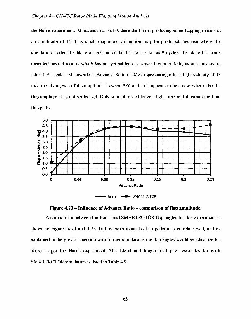
Chapter 4 - CH-47C Rotor Blade Flapping Motion Analysis
the Harris experiment. At advance ratio of 0, there the flap is producing some flapping motion at
an amplitude of 1°. This small magnitude of motion may be produced, because where the
simulation started the blade at rest and so far has ran as far as 9 cycles, the blade has some
unsettled inertial motion which has not yet settled at a lower flap amplitude, as one may see at
later flight cycles. Meanwhile at Advance Ratio of 0.24, representing a fast flight velocity of 33
m/s, the divergence of the amplitude between 3.6° and 4.6°, appears to be a case where also the
flap amplitude has not settled yet. Only simulations of longer flight time will illustrate the final
flap paths.
BO 01
2, •o 3 4 -
Q. F < a. to
LU
5.0 4.5 4.0
a.s 3.0
2.5 2.0 l.b 1.0 0.5 0.0
vtly.
I I I ' ' ' —^—•— I I I I —I—J—I—I— —1—L— I I I I
0.04 0.08 0.12
Advance Ratio
0.16 0.2 0.24
•Harris —I SMARTROTOR
Figure 4.23 - Influence of Advance Ratio - comparison of flap amplitude.
A comparison between the Harris and SMARTROTOR flap angles for this experiment is
shown in Figures 4.24 and 4.25. In this experiment the flap paths also correlate well, and as
explained in the previous section with further simulations the flap angles would synchronize in-
phase as per the Harris experiment. The lateral and longitudinal pitch estimates for each
SMARTROTOR simulation is listed in Table 4.9.
65
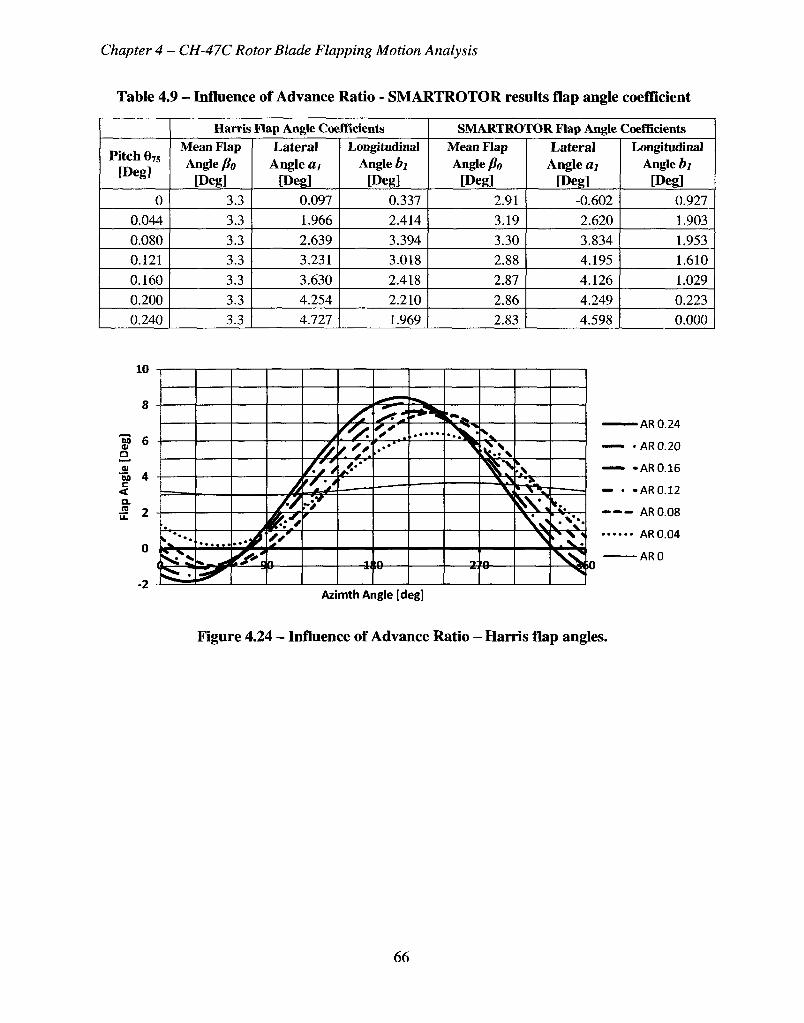
Chapter 4 - CH-47C Rotor Blade Flapping Motion Analysis
Table 4.9 - Influence of Advance Ratio - SMARTROTOR results flap angle coefficient
Pitch 875
[Deg]
0
0.044
0.080
0.121
0.160
0.200
0.240
Harris Flap Angle Coefficients Mean Flap Angle Po
[Deg]
3.3
3.3
3.3
3.3
3.3
3.3
3.3
Lateral Angle ai
[Deg]
0.097
1.966
2.639
3.231
3.630
4.254
4.727
Longitudinal Angle bi
[Deg]
0.337
2.414
3.394
3.018
2.418
2.210
1.969
SMARTROTOR Flap Angle Coefficients Mean Flap Angle po
[Deg]
2.91
3.19
3.30
2.88
2.87
2.86
2.83
Lateral Angle aj
[Deg]
-0.602
2.620
3.834
4.195
4.126
4.249
4.598
Longitudinal Angle bi
[Deg]
0.927
1.903
1.953
1.610
1.029
0.223
0.000
Azimth Angle [deg]
Figure 4.24 - Influence of Advance Ratio - Harris flap angles.
66
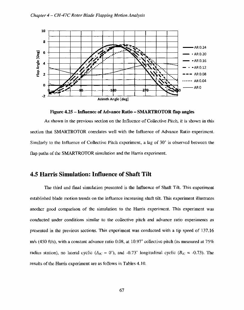
Chapter 4 - CH-47C Rotor Blade Flapping Motion Analysis
10
8
Azimth Angle [cleg]
Figure 4.25 - Influence of Advance Ratio - SMARTROTOR flap angles
As shown in the previous section on the Influence of Collective Pitch, it is shown in this
section that SMARTROTOR correlates well with the Influence of Advance Ratio experiment.
Similarly to the Influence of Collective Pitch experiment, a lag of 30° is observed between the
flap paths of the SMARTROTOR simulation and the Harris experiment.
4.5 Harris Simulation: Influence of Shaft Tilt
The third and final simulation presented is the Influence of Shaft Tilt. This experiment
established blade motion trends on the influence increasing shaft tilt. This experiment illustrates
another good comparison of the simulation to the Harris experiment. This experiment was
conducted under conditions similar to the collective pitch and advance ratio experiments as
presented in the previous sections. This experiment was conducted with a tip speed of 137.16
m/s (450 ft/s), with a constant advance ratio 0.08, at 10.97° collective pitch (as measured at 75%
radius station), no lateral cyclic (A/C = 0°), and -0.73° longitudinal cyclic (BIC = -0.73). The
results of the Harris experiment are as follows in Tables 4.10.
67
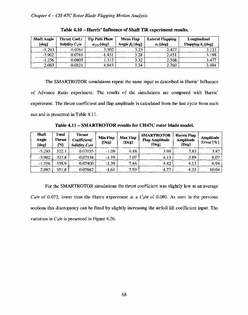
Chapter 4 - CH-47C Rotor Blade Flapping Motion Analysis
Table 4.10 - Harris' Influence of Shaft Tilt experiment results.
Shaft Angle tdegl
-5.293 -3.902 -1.256 2.083
Thrust Coef./ Solidity Cjla
0.0761 0.0781 0.0805 0.0821
Tip Path Plane aTpp [deg]
3.502 -1.451 1.312 4.843
Mean Flap Angle p0 [deg]
3.23 3.28 3.32 3.34
Lateral Flapping a, [deg]
2.427 2.451 2.568 2.760
Longitudinal Flapping bt [deg]
3.123 3.198 3.477 3.494
The SMARTROTOR simulations repeat the same input as described in Harris' Influence
of Advance Ratio experiment. The results of the simulations are compared with Harris'
experiment. The thrust coefficient and flap amplitude is calculated from the last cycle from each
run and is presented in Table 4.11.
Table 4.11 - SMARTROTOR results for CH47C rotor blade model.
Shaft Angle [deg]
-5.293
-3.902
-1.256
2.083
Total Thrust
[N]
322.1
327.8
338.9
351.8
Thrust Coefficient/ Solidity Cj/a
0.07035
0.07158
0.07400
0.07682
MinFlap [Deg]
-1.09
-1.19
-1.39
-1.61
Max Flap [Deg]
6.88
7.07
7.44
7.93
SMARTROTOR Flap Amplitude
[Deg]
3.98
4.13
4.42
4.77
Harris Flap Amplitude
[Deg]
3.83
3.89
4.13
4.33
Amplitude Error [%]
3.87
6.07
6.94
10.04
For the SMARTROTOR simulations the thrust coefficient was slightly low at an average
Cj/a of 0.072, lower than the Harris experiment at a Cj/a of 0.080. As seen in the previous
sections this discrepancy can be fixed by slightly increasing the airfoil lift coefficient input. The
variation in Cj/a is presented in Figure 4.26.
68

Chapter 4 - CH-47C Rotor Blade Flapping Motion Analysis
00
2 , > K5 o
<J
|t*H
n* .
- A -
•
-5 -4 -3 -2 -1 0
Shaft Tilt Angle [deg]
» Harris — • > SMARTROTOR
Figure 4.26 - Influence of Shaft Tilt - comparison of thrust coefficients.
The resultant flap amplitudes of the SMARTROTOR simulations are presented in Figure
.26. It is shown that the resultant flap amplitudes correlate well together.
v _ . - | s s s ^ - P « —— •D
"5. <
u_
• ' i
-6 -5 - 4 - 3 - 2 - 1 0 1 2 3
Shaft Tilt Angle [deg]
» Harris — » - SMARTROTOR
Figure 4.27 - Influence of Shaft Tilt - comparison of flap amplitude.
A comparison between the Harris and SMARTROTOR flap angles for this experiment is
shown in Figures 4.28 and 4.29. In this experiment, the flap paths also correlate well, and as
explained in the previous section with further simulations the flap angles would synchronize in-
phase as per the Harris experiment. The lateral and longitudinal pitch estimates for each
SMARTROTOR simulation is listed in Table 4.12.
69
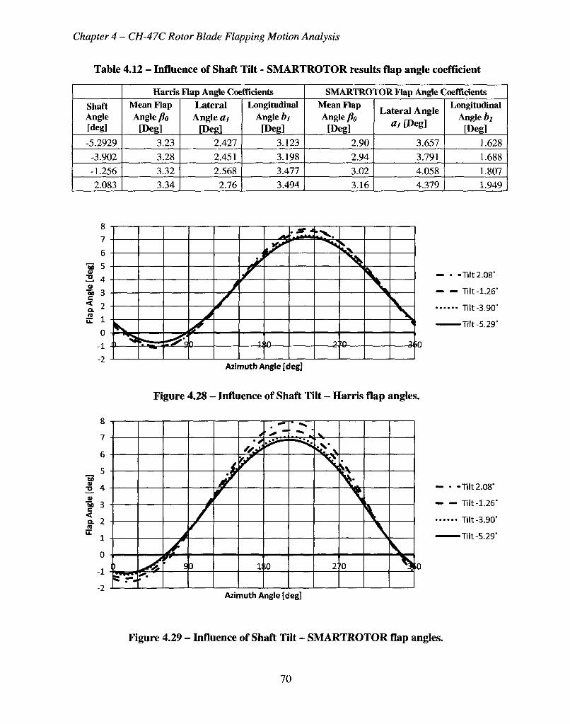
Chapter 4 - CH-47C Rotor Blade Flapping Motion Analysis
Table 4.12 - Influence of Shaft Tilt - SMARTROTOR results flap angle coefficient
Shaft Angle [deg]
-5.2929
-3.902
-1.256
2.083
Harris Flap Angle Coefficients Mean Flap Angle po
[Deg]
3.23
3.28
3.32
3.34
Lateral Angle ai
[Deg]
2.427
2.451
2.568
2.76
Longitudinal Angle bi
[Deg]
3.123
3.198
3.477
3.494
SMARTROTOR Flap Angle Coefficients Mean Flap Angle Po
[Deg]
2.90
2.94
3.02
3.16
Lateral Angle «i [Deg]
3.657
3.791
4.058
4.379
Longitudinal Angle bi
[Deg]
1.628
1.688
1.807
1.949
— • -Tilt 2.08°
— — Tilt-1.26"
Tilt-3.90°
Tilt-5.29°
Azimuth Angle [deg]
Figure 4.28 - Influence of Shaft Tilt - Harris flap angles.
— • -Tilt 2.08°
— — Tilt-1.26°
Tilt-3.90°
— T i l t -5.29°
.0
Azimuth Angle [deg]
Figure 4.29 - Influence of Shaft Tilt - SMARTROTOR flap angles.
70
eo c < a. to
s, 0
T ^ 3 11
-x>
f V
10
. 9 * ; > .
"*S<
^ >
T'f)
V \
^
\ >
31
M T3 _0J DO C < Q.
()
ft r*-t^f s 0
J
4
Y
I:
• >• T • > J > -
!0
V
< * ^ v
2
•
'0

Chapter 4 - CH-47C Rotor Blade Flapping Motion Analysis
As shown in the previous sections, it is shown in this section that SMARTROTOR
correlates well with the Influence of Shaft Tilt experiment. Similarly to the Influence of
Collective Pitch and Influence of Advance Ratio experiments, a lag of 30° is observed between
the flap paths of the SMARTROTOR simulation and the Harris experiment.
71
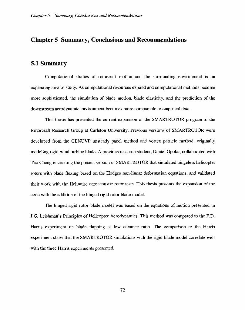
Chapter 5 - Summary, Conclusions and Recommendations
Chapter 5 Summary, Conclusions and Recommendations
5.1 Summary
Computational studies of rotorcraft motion and the surrounding environment is an
expanding area of study. As computational resources expand and computational methods become
more sophisticated, the simulation of blade motion, blade elasticity, and the prediction of the
downstream aerodynamic environment becomes more comparable to empirical data.
This thesis has presented the current expansion of the SMARTROTOR program of the
Rotorcraft Research Group at Carleton University. Previous versions of SMARTROTOR were
developed from the GENUVP unsteady panel method and vortex particle method, originally
modeling rigid wind turbine blade. A previous research student, Daniel Opoku, collaborated with
Tao Cheng in creating the present version of SMARTROTOR that simulated hingeless helicopter
rotors with blade flexing based on the Hodges non-linear deformation equations, and validated
their work with the Helinoise aeroacoustic rotor tests. This thesis presents the expansion of the
code with the addition of the hinged rigid rotor blade model.
The hinged rigid rotor blade model was based on the equations of motion presented in
J.G. Leishman's Principles of Helicopter Aerodynamics. This method was compared to the F.D.
Harris experiment on blade flapping at low advance ratio. The comparison to the Harris
experiment show that the SMARTROTOR simulations with the rigid blade model correlate well
with the three Harris experiments presented.
72
Chapter 5 - Summary, Conclusions and Recommendations
5.2 Conclusions
The hinged rigid blade model appears to work well as tested for forward flight helicopter
configurations. The comparison of the simulations to the three Harris experiments illustrated a
fair correlation between of flapping motions in forward flight at low advance ratios. The
comparison of the thrust data compared well, as did the flapping motion. The lead-lag frequency
was found to be at 20% the rotational velocity, which is consistent with the literature.
Since the thrust data compared well between the simulations and the Harris experiment, it
showed that the aerodynamics model worked well. The lift, drag and pitching moment data were
derived from their coefficient charts for speeds from Mach 0 to Mach 0.95. Adjustments to the
lift, drag and pitching moment input would be minor to correlate better with the Harris
experiment.
It remains to be seen if running the simulations longer, constructing a higher resolution of
blade aerodynamic grid nodes, and increasing the time step resolution would improve the
predictability of the simulation. Discrepancies between the flap amplitudes of the simulations
and the Harris experiment will need to be clarified when these simulations are re-run for longer
duration to ensure that the flap motion has settled. The assumption that the blade acts as rigid
blade appears to work well, since blade deformations will be small, and are suitable for the rigid
blade articulated hub model.
5.3 Recommendations
The SMARTROTOR program can continue to be amended and expanded upon. The
SMARTROTOR program, written in Fortran 77 is a challenging program to amend. It is the
intention of this author to provide some guidance to future users by providing a brief guide to
73
Chapter 5 - Summary, Conclusions and Recommendations
how to operate the SMARTROTOR program in Appendix A of this Thesis. Comment lines by
this author and previous authors embedded throughout the SMARTROTOR source code will
guide one through the workings of this program.
One challenging area of the code that may require some corrections is the wake model.
One should amend the aerodynamic section of the code so that if one is only concerned with the
aerodynamic effects occurring within the zone of the rotor blades, and one can turn off the wake
being generated downstream of the blade. This would reduce the computational time required to
run these simulations as their wake aft of the rotor blades would not be infinitely increasing in
complexity over time. It may appear that there are existing variables in the aerodynamic input
finals that can be adjusted to accomplish this.
Once it is determined that the simulations can be run with the wake model for longer
flight time, re-simulation of the Harris experiment may be in order. This will confirm or illustrate
any other problems regarding whether the flap motions of simulations will settle in-phase with
the Harris experiment. A comparison with other models and existing data would be useful to
further illustrate the validation of the rigid blade model based on the equations of motion
presented in Leishman.
With further study of both the rigid code based on the equations of motion presented by
Leishman, and the hingeless Hodges equations, one may be able to couple both models together
properly to have a hinged rotor blade model with blade deformation. Based on the methods or
rearranging the SMARTROTOR code listed in this Thesis, there are opportunities for the
addition of other structural blade model codes to couple with the GENUVP aerodynamics model.
74
References
References
[1] J.G. Leishman, Principles of Helicopter Aerodynamics, Cambridge University Press, New
York, NY, 2000.
[2] Bartha, M. and Madzer, J. 1913. "Schraubenflugelanordnung fur Luftschraubenpaare," Patent
No. 249,702.
[3] J.R. Chiles, The God Machine, Bantam Dell, A Division of Random House, Inc., New York,
New York, 2007.
[4] Domke, B. 2011, Aviation Images - Aircraft in Detail - Helicopter Rotorhead Gallery,
http://www.b-domke.de/AviationImages/Rotorhead.html (current August 2011).
[5] Bauchau O.A., Bottasso C.L. and Nikishkov Y.G.: "Modeling Rotorcraft Dynamics with
Finite Element Multibody Procedures." Mathematical and Computer Modeling, 33, pp 1113 —
1137,2001.
[6] Johnson, W. "Rotorcraft Aerodynamic Models for a Comprehensive Analysis." American
Helicopter Society 54th Annual Forum, Washington, D.C., May 1998.
[7] D.A. Wachspress, T.R. Quackenbush, and A.H. Boschitsch, "Rotorcraft Interactional
Aerodynamics Calculations with Fast Vortex / Fast Panel Methods", American Helicopter
Society 56th Annual Forum, Virginia Beach, VA, May 2-4, 2000.
[8] D. Opoku, "Aeroelastic and aeroacoustic modeling of rotorcraft," Master's thesis, Carleton
University, 2002.
[9] F.D. Harris, "Articulated Rotor Blade Flapping Motion at Low Advance Ratios", Journal of
the American Helicopter Society, 17(1), pp. 41-48, 1972.
75
References
[10] T. Cheng, "Structural Dynamics Modeling of Helicopter Blades for Computational
Aeroelasticity," Master's thesis, Massachusetts Institute of Technology, May 2002.
[11] S.G. Voutsinas, A GENeralized Unsteady Vortex Particle Method for Solving the Unsteady
Flow around Multi-component Configurations, Fluids Section - Dept. of Mechanical
Engineering, National Technical University of Athens, Greece, 1990.
[12] D.G. Triantor, Aerodynamic and Aeroacoustic Analysis of Helicopter Rotors, PhD
dissertation, Fluids Section - Dept. of Mechanical Engineering, National Technical University of
Athens, Greece, 2002.
[13] S.G. Voutsinas, "Vortex methods in aeronautics: how to make things work", International
Journal of Computational Fluid Dynamics, Vol. 20 No. 1 pp. 3-18, January 2006.
[14] D.H. Hodges, "A Mixed Variational Formulation based on Exact Intrinsic Equations for
Dynamics of Moving Beam", International Journal of Solids and Structures, vol. 26, no. 11, pp.
1253-1273, 1990.
[15] P.P. Friedmann and F.X. Bagnoud, "Rotary Wing Aeroelasticity - A Historical Perspective
and Some Current Trends", Journal of Aircraft, vol 40, no. 6, pp. 1019-1046, 2003.
[16] X. Shang, Aeroelastic Stability of Composite Hingeless Rotors with Finite-State Unsteady
Aerodynamics, PhD dissertation, School of Aerospace Engineering, Georgia Institute of
Technology, Atlanta, Georgia, 1995.
[17] W.R. Splettstoesser et al. 'The HELINOISE Aeroacoustic Rotor Test in the NDW - Test
Documentation and Representative Results", DLR-Mitt. 93-09, DLR, Braunschweig, Germany,
1993.
[18] M. Ghorashi, Dynamics of Elastic Nonlinear Rotating Composite Beams with Embedded
Actuators, PhD dissertation, Carleton University, 2009.
76
References
[19] Alan Hindmarsh, ODEPACK, a Systematized Collection of ODE Solvers, in Scientific
Computing, Elsevier, 1983. Program code available at http://people.sc.fsu.edu/~jburkardt/
f77_src/odepack/odepack.html (Current August 2011).
[20] Mark W. Spong et al, Robot Modeling and Control, John Wiley & Sons, Inc., 2006.
[21] Dadone, L.U. "U.S. Army Helicopter Design Datcom Volume 1 Airfoils", U.S. Army Air
Mobility Research and Development Laboratory, Aviations Systems Command, September
1976.
[22] Abbott, I.H. and Von Doenhoff, Theory of Wing Sections Including a Summary of Airfoil
Data, Dover Publications, Inc. 1949.
[23] Gessow, A. and Myers, G.C., Jr. 1952, Aerodynamics of the Helicopter, Macmillon Co.,
Republished by Frederick Ungar Publishing, New York, NY, 1967.
77
Appendix A SMARTROTOR User's Guide and Input Files
Appendix A SMARTROTOR User's Guide and Input Files
The Appendix summarizes how to use and operate SMARTROTOR. This is a
preliminary guide to set-up and ran the most basic helicopter simulations. SMARTROTOR has
other capabilities regarding simulating helicopter noise, and activating the Active Twist Control.
This guide should allow users to ran hingeless deformed, hinged rigid, and deformed hinged
simulations.
A.1 SMARTROTOR Operators Guide
The program SMARTROTOR consists of several files to run. The home folder for the
SMARTROTOR code is located in a folder entitled "SMARTROTOR". This directory contains
the following important files:
• the Fortran 77 sources files entitled with suffix ".f"
• the Fortran 77 object files entitled with suffix ".o"
• the executable program SMARTROTOR.exe
• the make file entitled "makefile", contains the list of source and objects files used for
compliling.
• The Input/Output file Directories
o HARRIS_CH47 - contains the input and output files related to the Harris
experiment simulations.
o BO_105_FTNAL.70 - contains the input and output files related to the Helioise
experiment simulations.
78
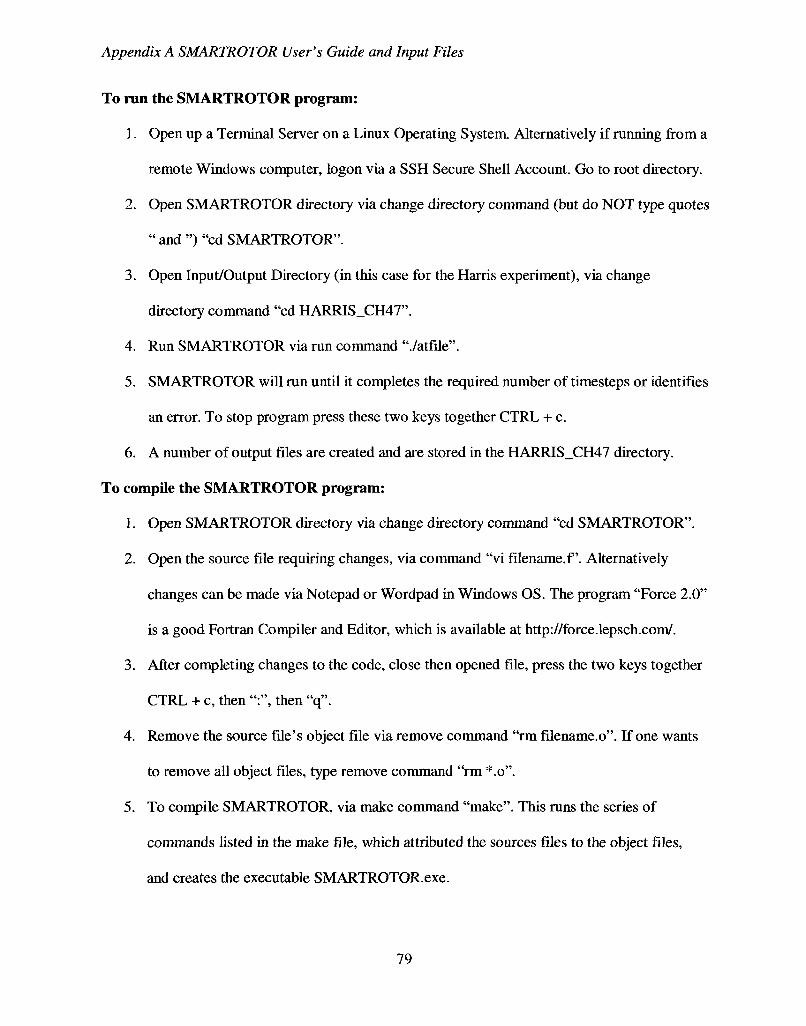
Appendix A SMARTROTOR User's Guide and Input Files
To ran the SMARTROTOR program:
1. Open up a Terminal Server on a Linux Operating System. Alternatively if running from a
remote Windows computer, logon via a SSH Secure Shell Account. Go to root directory.
2. Open SMARTROTOR directory via change directory command (but do NOT type quotes
" and ") "cd SMARTROTOR".
3. Open Input/Output Directory (in this case for the Harris experiment), via change
directory command "cd HARRIS_CH47".
4. Run SMARTROTOR via run command "./atfile".
5. SMARTROTOR will run until it completes the required number of timesteps or identifies
an error. To stop program press these two keys together CTRL + c.
6. A number of output files are created and are stored in the HARRIS_CH47 directory.
To compile the SMARTROTOR program:
1. Open SMARTROTOR directory via change directory command "cd SMARTROTOR".
2. Open the source file requiring changes, via command "vi filename.f'. Alternatively
changes can be made via Notepad or Wordpad in Windows OS. The program "Force 2.0"
is a good Fortran Compiler and Editor, which is available at http://force.lepsch.com/.
3. After completing changes to the code, close then opened file, press the two keys together
CTRL + c, then ":", then "q".
4. Remove the source file's object file via remove command "rm filename.o". If one wants
to remove all object files, type remove command "rm *.o".
5. To compile SMARTROTOR, via make command "make". This runs the series of
commands listed in the make file, which attributed the sources files to the object files,
and creates the executable SMARTROTOR.exe.
79
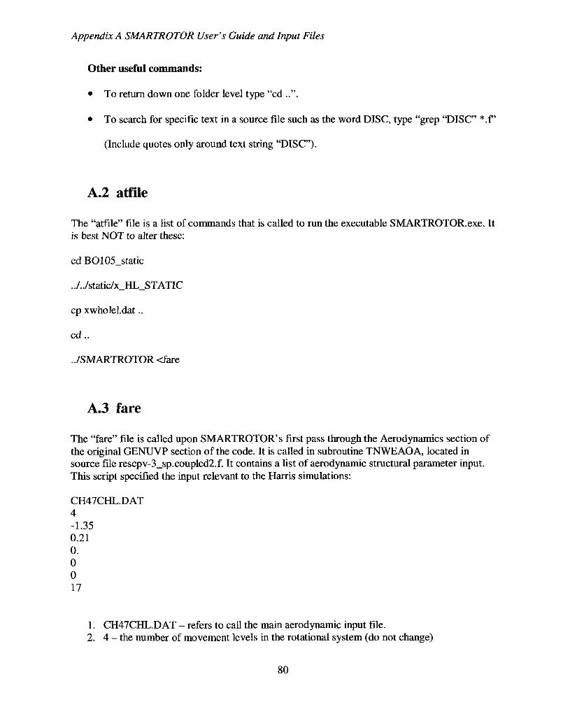
Appendix A SMARTROTOR User's Guide and Input Files
Other useful commands:
• To return down one folder level type "cd ..".
• To search for specific text in a source file such as the word DISC, type "grep "DISC" *.f
(Include quotes only around text string "DISC").
A.2 atfile
The "atfile" file is a list of commands that is called to run the executable SMARTROTOR.exe. It is best NOT to alter these:
cd BO105_static
../../static/x_HL_STATIC
cp xwholel.dat..
cd..
../SMARTROTOR <fare
A.3 fare
The "fare" file is called upon SMARTROTOR's first pass through the Aerodynamics section of the original GENUVP section of the code. It is called in subroutine TNWEAOA, located in source file rescpv-3_sp.coupled2.f. It contains a list of aerodynamic structural parameter input. This script specified the input relevant to the Harris simulations:
CH47CHL.DAT 4 -1.35 0.21 0. 0 0 17
1. CH47CHL.DAT - refers to call the main aerodynamic input file. 2. 4 - the number of movement levels in the rotational system (do not change)
80
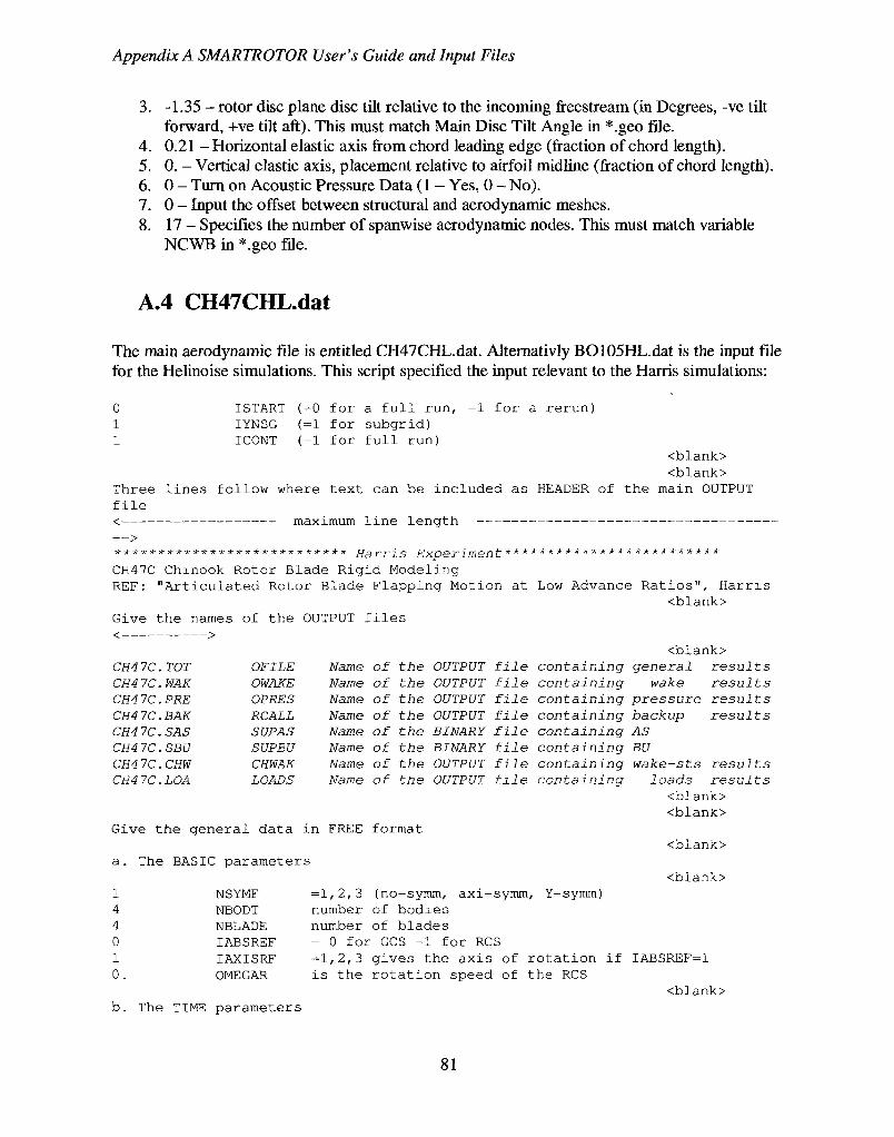
Appendix A SMARTROTOR User's Guide and Input Files
3. -1.35 - rotor disc plane disc tilt relative to the incoming freestream (in Degrees, -ve tilt forward, +ve tilt aft). This must match Main Disc Tilt Angle in *.geo file.
4. 0.21 - Horizontal elastic axis from chord leading edge (fraction of chord length). 5. 0. - Vertical elastic axis, placement relative to airfoil midline (fraction of chord length). 6. 0 - Turn on Acoustic Pressure Data (1 - Yes, 0 - No). 7. 0 - Input the offset between structural and aerodynamic meshes. 8. 17 - Specifies the number of spanwise aerodynamic nodes. This must match variable
NCWB in *.geo file.
A.4 CH47CHL.dat
The main aerodynamic file is entitled CH47CHL.dat. Alternativly BO105HL.dat is the input file for the Helinoise simulations. This script specified the input relevant to the Harris simulations:
0 ISTART (=0 for a full run, =1 for a rerun) 1 IYNSG (=1 for subgrid) 1 ICONT (=1 for full run)
<blank> <blank>
Three lines follow where text can be included as HEADER of the main OUTPUT file < maximum line length — > *************************** Harris Experiment ************************* CH47C Chinook Rotor Blade Rigid Modeling REF: "Articulated Rotor Blade Flapping Motion at Low Advance Ratios", Harris
<blank> Give the names of the OUTPUT files
<blank> Name of the OUTPUT file containing general results Name of the OUTPUT file containing wake results Name of the OUTPUT file containing pressure results Name of the OUTPUT file containing backup results Name of the BINARY file containing AS Name of the BINARY file containing BU Name of the OUTPUT file containing wake-sts results Name of the OUTPUT file containing loads results
<blank>
CH4 7C. CH4 7C. CH4 7C. CH4 7C. CH4 7C. CH4 7C. CH4 7C. CH4 7C.
.TOT ,WAK .PRE .BAR SAS
.SBU ,CHW .LOA
OFILE OWAKE OPRES RCALL SUP AS SUPBU CHWAK LOADS
Give the general data in FREE format
a. The BASIC parameters
=1,2,3
<blank>
<blank>
<blank> 1 4 4 0 1 0.
NSYMF NBODT NBLADE IABSREF IAXISRF OMEGAR
(no-symm, axi-symm, Y-symm) number of bodies number of blades = 0 for GCS =1 for RCS =1,2,3 gives the axis of rotation if IABSREF=1 is the rotation speed of the RCS
<blank> b. The TIME parameters
81
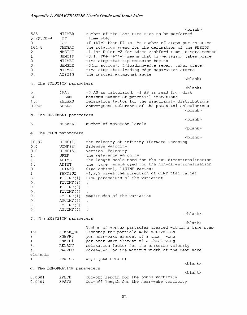
Appendix A SMARTROTOR User's Guide and Input Files
525 5.2952E-4 0 164.8 2 1 0 0 0 0.
NTIMER DT IDT OMEGAT NMETHT NEMTIP NTIMET NEMSLE NTIMEL AZIMIN
<blank> number of the last time step to be performed time step if IDT=1 then DT is the number of steps per rotation the rotation speed for the definition of the PERIOD =1 for Euler =2 for Adams Bashford time Integra scheme =0,1. The latter means that tip-emission takes place time step that tip-emission begins =0 (no action), 1(leading-edge separ. takes place) time step that leading-edge separation starts the initial azimuthal angle
<blank> The SOLUTION parameters
<blank> =0 AS is calculated, =1 AS is read from disk maximum number of potential iterations relaxation factor for the singularity distributions convergence tolerance of the potential calculations
<blank> The MOVEMENT parameters
<blank> number of movement levels
<blank>
0 50 1.0 0.005
I MAT I TERM RELAXS EPSDS
NLEVELT
e. The FLOW parameters
10.97 0.0 0.0 1. 1. 1. 0 1 0. 0. 0. 0. 0. 0. 0. 0.
UINF(l) UINF(2) UINF(3) UREF ADIML ADIMT IUINFC IAXISUI TIUINF(l) TIUINF(2) TIUINF(3) TIUINF(4) AMUINF(l) AMUINF(2) AMUINF(3) AMUINF(4)
<blank> the velocity at infinity (Forward incoming Sideways Velocity Vertical Velocity the reference velocity the length scale used for the non-dimentionalisation the time scale used for the non-dimentionalisation 0(no action), 1(UINF varies) =1,2,3 gives the direction of UINF that varies time parameters of the variation
amplitudes of the variation
<blank> f. The EMISSION parameters
150 1
1 i
1. elements 1
N_WAK_ON NNEVP0 NNEVP1 RELAXU PARVEC
NEMISS
<blank> Number of vortex particles created within a time step Timestep for particle wake activation per near-wake element of a thin wing per near-wake element of a thick wing relaxation factor for the emission velocity parameter for the minimum width of the near-wake
<blank> =0,1 (See CREATE)
g. The DEFORMATION parameters <blank>
0.0001 EPSFB Cut-off length for the bound vorticity C.0001 EPSFW Cut-off length for the near-wake vorticity
82
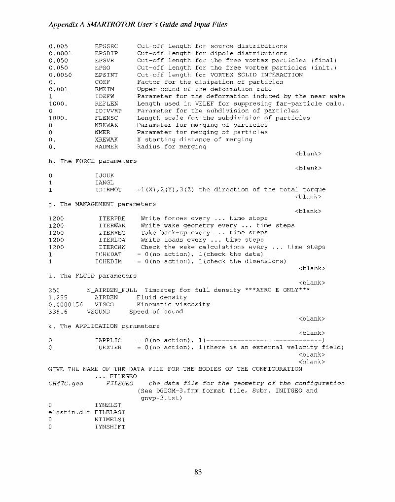
Appendix A SMARTROTOR User's Guide and Input Files
0.005 0.0001 0.050 0.050 0.0050 0. 0.001 1 1000. 0 1000. 0 0 0. 0.
EPSSRC EPSDIP EPSVR EPSO EPSINT COEF RMETM IDEFW REFLEN IDIWRP FLENSC NREWAK NMER XREWAK RADMER
Cut-off length for source distributions Cut-off length for dipole distributions Cut-off length for the free vortex particles (final) Cut-off length for the free vortex particles (init.) Cut-off length for VORTEX SOLID INTERACTION Factor for the disipation of particles Upper bound of the deformation rate Parameter for the deformation induced by the near wake Length used in VELEF for suppresing far-particle calc. Parameter for the subdivision of particles Length scale for the subdivision of particles Parameter for merging of particles Parameter for merging of particles X starting distance of merging Radius for merging
<blank> h. The FORCE parameters
<blank> IJOUK IANGL IDIRMOT =1(X),2(Y),3(Z) the direction of the total torque
<blank> The MANAGEMENT parameters
<blank> 1200 1200 1200 1200 1200 1 1
ITERPRE ITERWAK ITERREC ITERLOA ITERCHW ICHEDAT ICHEDIM
Write forces every ... time steps Write wake geometry every ... time steps Take back-up every ... time steps Write loads every ... time steps Check the wake calculations every ... = 0(no action), 1(check the data) = 0(no action), 1(check the dimensions)
time steps
<blank> i. The FLUID parameters
<blank> 250 N_AIRDEN_FULL Timestep for full density ***AERO-E ONLY*** 1.255 AIRDEN Fluid density 0.0000156 VISCO Kinematic viscosity 338.6 VSOUND Speed of sound
k. The APPLICATION parameters <blank>
<blank> IAPPLIC IUEXTER
= 0(no action), = 0(no action),
K-1(there is an external velocity field)
<blank> <blank>
GIVE THE NAME OF THE DATA FILE FOR THE BODIES OF THE CONFIGURATION ... FILEGEO
CH47C.geo FILEGEO the data file for the geometry of the configuration (See DGEOM-3.frm format file, Subr. INITGEO and gnvp-3.txt)
0 IYNELST elastin.dlr FILELAST
NTIMELST IYNSHIFT
83
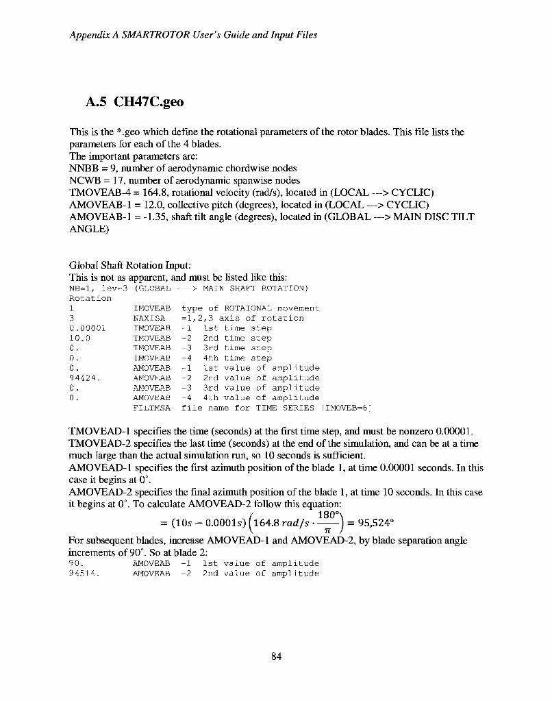
Appendix A SMARTROTOR User's Guide and Input Files
A.5 CH47C.geo
This is the *.geo which define the rotational parameters of the rotor blades. This file lists the parameters for each of the 4 blades. The important parameters are: NNBB = 9, number of aerodynamic chordwise nodes NCWB = 17, number of aerodynamic spanwise nodes TMOVEAB-4 = 164.8, rotational velocity (rad/s), located in (LOCAL — > CYCLIC) AMOVEAB-1 = 12.0, collective pitch (degrees), located in (LOCAL —> CYCLIC) AMOVEAB-1 = -1.35, shaft tilt angle (degrees), located in (GLOBAL —> MAIN DISC TILT ANGLE)
Global Shaft Rotation Input: This is not as apparent, and must be listed like this:
MAIN SHAFT ROTATION)
t y p e of ROTAIONAL movement 1 , 2 , 3 a x i s o f r o t a t i o n
1 s t t i m e s t e p 2nd t i m e s t e p 3 r d t i m e s t e p 4 t h t i m e s t e p 1 s t v a l u e o f a m p l i t u d e 2nd v a l u e of a m p l i t u d e 3 r d v a l u e o f a m p l i t u d e 4 t h v a l u e o f a m p l i t u d e
name f o r TIME SERIES [IMOVEB=6]
TMOVEAD-1 specifies the time (seconds) at the first time step, and must be nonzero 0.00001. TMOVEAD-2 specifies the last time (seconds) at the end of the simulation, and can be at a time much large than the actual simulation run, so 10 seconds is sufficient. AMOVEAD-1 specifies the first azimuth position of the blade 1, at time 0.00001 seconds. In this case it begins at 0°. AMOVEAD-2 specifies the final azimuth position of the blade 1, at time 10 seconds. In this case it begins at 0°. To calculate AMOVEAD-2 follow this equation:
. / 180°\ = (10s - 0.0001s) f 164.8 rad/s J = 95,524°
For subsequent blades, increase AMOVEAD-1 and AMOVEAD-2, by blade separation angle increments of 90°. So at blade 2: 90. AMOVEAB -1 1st value of amplitude 94514. AMOVEAB -2 2nd value of amplitude
NB=1, lev=3 Rotation 1 3 0.00001 10.0 0. 0. 0. 94424. 0. 0.
(GLOBAL
IMOVEAB NAXISA TMOVEAB TMOVEAB TMOVEAB TMOVEAB AMOVEAB AMOVEAB AMOVEAB AMOVEAB FILTMSA
>
type =1,2 -1 -2 -3 -4 -1 -2 -3 -4 file
84

Appendix A SMARTROTOR User's Guide and Input Files
***CH47C bl ***LEVEL 5
Body Number
2 9 17 0 0 2 2 3 1 0 0 3
ade, THIN WING, *** MOVEMENT,
<blank> NB = 1-<blank>
NLIFT (nb=l) NNBB (nb=l) NCWB (nb=l) NNBBTHL NCWBTHL active for thick wings only
Number of Chordwise Nodes Number of Spanwise Nodes
active for thick wings only
Give data NB=1, lev=2 Rotation 13 2 0.00001 0. 0. 164.8 19.36 0.0 -0.73 90.
Translation 1 \ 0.00001 10.0
NB=1, lev Rotation 1 3 0.00001 10.0 0. 0. 0.
IYNTIPS (nb=l) IYNLES (nb=l) NELES (nb=l) IDIRMOB (nb=l) direction for the torque calculation
<blank> LEVEL (nb=l) the level of movement (MAIN ROTOR, CYCLIC,TILT)
<blank> for every level (LOCAL > CYCLIC)
IMOVEAB NAXISA TMOVEAB TMOVEAB TMOVEAB TMOVEAB AMOVEAB AMOVEAB AMOVEAB AMOVEAB FILTMSA (N/A) IMOVEUB NAXISU TMOVEUB TMOVEUB TMOVEUB TMOVEUB AMOVEUB AMOVEUB AMOVEUB AMOVEUB FILTMSU —> ROOT
IMOVEAB NAXISA TMOVEAB TMOVEAB TMOVEAB TMOVEAB AMOVEAB
type of ROTAIONAL movement =1,2,3 axis of rotation -1 1st time step -2 2nd time step -3 3rd time step -4 4th time step -1 1st value of amplitude COLLECTIVE -2 2nd value of amplitude COS CYCLIC -3 3rd value of amplitude SIN CYCLIC -4 4th value of amplitude file name for TIME SERIES [IMOVEB=6]
type of TRANSLATIONAL movement =1,2,3 axis of translation -1 1st time step
2nd time step 3rd time step 4th time step 1st value of amplitude 2nd value of amplitude 3rd value of amplitude 4th value of amplitude
file name for TIME SERIES [IMOVEB=6] CUTOUT
type of ROTAIONAL movement =1,2,3 axis of rotation -1 1st time step -2 2nd time step -3 3rd time step -4 4th time step -1 1st value of amplitude
-2 -3 -4 -1 -2 _3 -4
85
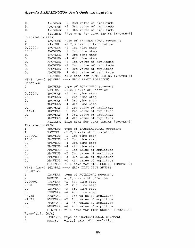
Appendix A SMARTROTOR User's Guide and Input Files
0. 0 . 0 .
Translation 1 2 0.00001 10.0 0. 0. 0. 0. 0. 0.
NB=1, lev=3 Rotation 1 3 0.00001 10.0 0. 0. 0. 94424. 0. 0.
Translation 1 1 0.00001 10.0 0. 0. 0. 0. 0. 0.
NB=1, lev=4 Rotation 1 2 0.00001 10.0 0. 0 . -1.35 -1.35 0.
Translation 1
AMOVEAB AMOVEAB AMOVEAB FILTMSA (N/A) IMOVEUB NAXISU TMOVEUB TMOVEUB TMOVEUB TMOVEUB AMOVEUB AMOVEUB AMOVEUB AMOVEUB FILTMSU (GLOBAL
IMOVEAB NAXISA TMOVEAB TMOVEAB TMOVEAB TMOVEAB AMOVEAB AMOVEAB AMOVEAB AMOVEAB FILTMSA (N/A) IMOVEUB NAXISU TMOVEUB TMOVEUB TMOVEUB TMOVEUB AMOVEUB AMOVEUB AMOVEUB AMOVEUB FILTMSU (GLOBAL
IMOVEAB NAXISA TMOVEAB TMOVEAB TMOVEAB TMOVEAB AMOVEAB AMOVEAB AMOVEAB AMOVEAB FILTMSA (N/A) IMOVEUB NAXISU
-2 2nd value of amplitude -3 3rd value of amplitude -4 4th value of amplitude file name for TIME SERIES [IMOVEB=6]
type of TRANSLATIONAL movement =1,2,3 axis of translation -1 1st time step -2 2nd time step -3 3rd time step -4 4th time step -1 1st value of amplitude -2 2nd value of amplitude -3 3rd value of amplitude -4 4th value of amplitude file name for TIME SERIES [IMOVEB=6] > MAIN SHAFT ROTATION)
type of ROTAIONAL movement =1,2,3 axis of rotation -1 1st time step -2 2nd time step -3 3rd time step -4 4th time step -1 1st value of amplitude -2 2nd value of amplitude -3 3rd value of amplitude -4 4th value of amplitude file name for TIME SERIES [IMOVEB=6]
type of TRANSLATIONAL movement =1,2,3 axis of translation -1 1st time step -2 2nd time step -3 3rd time step -4 4th time step -1 1st value of amplitude -2 2nd value of amplitude -3 3rd value of amplitude -4 4th value of amplitude file name for TIME SERIES [IMOVEB=6] > MAIN DISC TILT ANGLE)
type of ROTAIONAL movement =1,2,j axis of rotation -1 1st time step -2 2nd time step -3 3rd time step -4 4th time step -1 1st value of amplitude -2 2nd value of amplitude -3 3rd value of amplitude -4 4th value of amplitude file name for TIME SERIES [IMOVEB=6]
type of TRANSLATIONAL movement =1,2,3 axis of translation
86
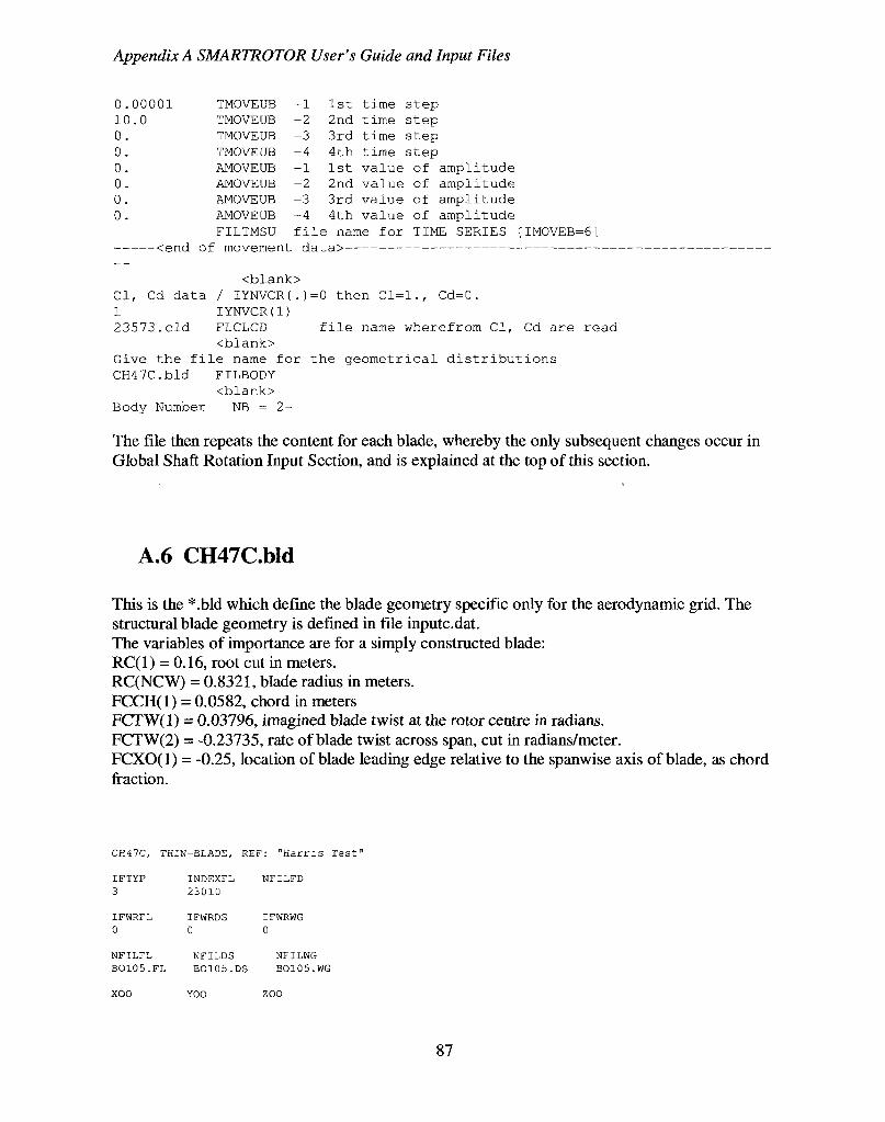
Appendix A SMARTROTOR User's Guide and Input Files
0 . 0 0 0 0 1 1 0 . 0 0 . 0 . 0 . 0 . 0 . 0 .
< p n d
TMOVEUB TMOVEUB TMOVEUB
TMOVEUB AMOVEUB AMOVEUB AMOVEUB AMOVEUB
FILTMSU o f m o v e m e n
- 1 - 2 - 3 - 4 - 1 - 2 - 3 - 4
f i t d
1st time step 2nd time step 3rd time step 4th time step 1st value of amplitude 2nd value of amplitude 3rd value of amplitude 4th value of amplitude
file name for TIME SERIES [IMOVEB=6]
<blank> CI, Cd data / IYNVCR(.)=0 then Cl=l., Cd=0. 1 IYNVCR(1) 23573.eld FLCLCD file name wherefrom CI, Cd are read
<blank> Give the file name for the geometrical distributions CH4 7C.bld FILBODY
<blank> Body Number NB = 2-
The file then repeats the content for each blade, whereby the only subsequent changes occur in Global Shaft Rotation Input Section, and is explained at the top of this section.
A.6 CH47C.bld
This is the *.bld which define the blade geometry specific only for the aerodynamic grid. The structural blade geometry is defined in file inputc.dat. The variables of importance are for a simply constructed blade: RC(1) = 0.16, root cut in meters. RC(NCW) = 0.8321, blade radius in meters. FCCH(l) = 0.0582, chord in meters FCTW(l) = 0.03796, imagined blade twist at the rotor centre in radians. FCTW(2) = -0.23735, rate of blade twist across span, cut in radians/meter. FCXO(l) = -0.25, location of blade leading edge relative to the spanwise axis of blade, as chord fraction.
CH47C, THIN-BLADE, REF: "Harris Test"
IFTYP 3
IFWRFL 0
NFILFL B O 1 0 5 . F L
INDEXFL 2 3 0 1 0
IFWRDS 0
NFILDS BO105.DS
NFILFD
IFWRWG 0
NFILWG BO105.WG
xoo YOO ZOO
87
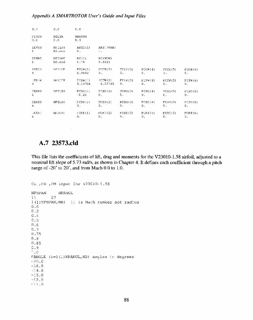
Appendix A SMARTROTOR User's Guide and Input Files
o.o 0 .0 0 .0
PITCH 0.0
IEXKS 1
IEXRC 1
IEXCH 4
IEXTW 4
IEXXO 4
IEXZO 4
IEXRT 4
DELTA 0.0
NFILKS KS.nod
NFILRC BO.nod
NFILCH
NFILTW
NFILXO
NFILZO
NFILRT
WNGANG 0.0
AKSI(l) 0.
RC(1) 0.16
FCCH(l) 0.0582
FCTW(l) 0.03796
FCXO(1) -0.25
FCZO(l) 0.
FCRT(l) 0.
AKSI(NNB) 1.
RC(NCW) 0.8321
FCCH(2) 0.
FCTW(2) -0.23735
FCXO(2) 0.
FCZO(2) 0.
FCRT(2) 0.
FCCH(3) 0.
FCTW(3) 0.
FCXO(3) 0.
FCZO(3) 0.
FCRT(3) 0.
FCCH(4) 0.
FCTW(4) 0.
FCXO(4) 0.
FCZO(4) 0.
FCRT(4) 0.
FCCH(5) 0.
FCTW(5) 0.
FCXO(5) 0.
FCZO(5) 0.
FCRT(5) 0.
FCCH(6) 0.
FCTW(6) 0.
FCXO(6) 0.
FCZO(6) 0.
FCRT(6) 0.
A.7 23573.cld
This file lists the coefficients of lift, drag and moments for the V23010-1.58 airfoil, adjusted to a nominal lift slope of 5.73 rad/s, as shown in Chapter 4. It defines each coefficient through a pitch range of-20° to 20°, and from Mach 0.0 to 1.0.
CL ,CD ,CM input for V23010-1.58
NPSPAN NPANGL 11 27 1(1)NPSPAN,NB) it is Mach number not radius 0.0 0.2 0.4 0.5 0.6 0.7 0.75 0.8 0.85 C.9 1 .0 PANGLE (I=1(1)NPANGL,NB) angles in degrees -20.0 -16.0 -14.0 -13.0 -12.0
88
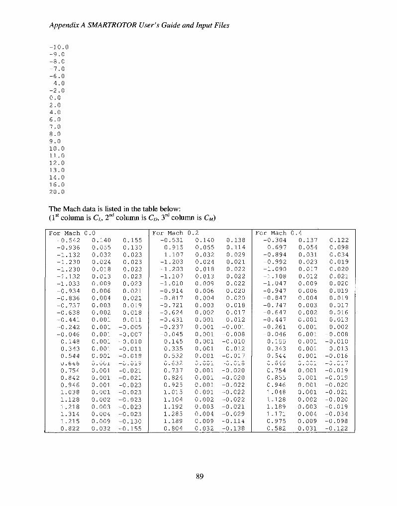
Appendix A SMARTROTOR User's Guide and Input Files
- 1 0 . 0 - 9 . 0 - 8 . 0 - 7 . 0 - 6 . 0 - 4 . 0 - 2 . 0 0 . 0 2 . 0 4 . 0 6 . 0 7 . 0 8 . 0 9 . 0 1 0 . 0 1 1 . 0 1 2 . 0 13 .0 1 4 . 0 16 .0 20 .0
The Mach data is listed in the table below: (1st column is Cu 2nd column is CD, 3rd column is CM)
F o r Mach - 0 . 5 4 2 - 0 . 9 3 6 - 1 . 1 3 2 - 1 . 2 3 0 - 1 . 2 3 0 - 1 . 1 3 2 - 1 . 0 3 3 - 0 . 9 3 4 - 0 . 8 3 6 - 0 . 7 3 7 - 0 . 6 3 8 - 0 . 4 4 1 - 0 . 2 4 2 - 0 . 0 4 6
0 . 1 4 8 0 . 3 4 3 0 . 5 4 4 u . 6^6 0 . 7 5 4 0 . 8 4 2 0 . 9 4 6 1 . 0 3 8 1 . 1 2 8 1 . 2 1 8 1 . 3 1 4 1 . 2 1 5 0 . 8 2 2
0 . 0 0 . 1 4 0 0 . 0 5 5 0 . 0 3 2 0 . 0 2 4 0 . 0 1 8 0 . 0 1 3 0 . 0 0 9 0 . 0 0 6 0 . 0 0 4 0 . 0 0 3 0 . 0 0 2 0 . 0 0 1 0 . 0 0 1 0 . 0 0 1 0 . 0 0 1 0 . 0 0 1 0 . 0 0 1 0 . Oux 0 . 0 0 1 0 . 0 0 1 0 . 0 0 1 0 . 0 0 1 0 . 0 0 2 0 . 0 0 3 0 . 0 0 4 0 . 0 0 9 0 . 0 3 2
0 . 1 5 5 0 . 1 3 0 0 . 0 2 3 0 . 0 2 3 0 . 0 2 3 0 . 0 2 3 0 . 0 2 3 0 . 0 2 1 0 . 0 2 1 0 . 0 1 9 0 . 0 1 8 0 . 0 1 1
- 0 . 0 0 5 - 0 . 0 0 7 - 0 . 0 1 0 - 0 . 0 1 1 - 0 . 0 1 8 —0.013 - 0 . 0 2 1 - 0 . 0 2 1 - 0 . 0 2 3 - 0 . 0 2 3 - 0 . 0 2 3 - 0 . 0 2 3 - 0 . 0 2 3 - 0 . 1 3 0 - 0 . 1 5 5
F o r Mach - 0 . 5 3 1 - 0 . 9 1 5 - 1 . 1 0 7 - 1 . 2 0 3 - 1 . 2 0 3 - 1 . 1 0 7 - 1 . 0 1 0 - 0 . 9 1 4 - 0 . 8 1 7 - 0 . 7 2 1 - 0 . 6 2 4 - 0 . 4 3 1 - 0 . 2 3 7 - 0 . 0 4 5
0 . 1 4 5 0 . 3 3 5 0 . 5 3 2 0 . 6 3 2 0 . 7 3 7 0 . 8 2 4 0 . 9 2 5 1 . 0 1 5 1 . 1 0 4 1 . 1 9 2 1 . 2 8 5 1 . 1 8 9 0 . 8 0 4
0 . 2 0 . 1 4 0 0 . 0 5 5 0 . 0 3 2 0 . 0 2 4 0 . 0 1 8 0 . 0 1 3 0 . 0 0 9 0 . 0 0 6 0 . 0 0 4 0 . 0 0 3 0 . 0 0 2 0 . 0 0 1 0 . 0 0 1 0 . 0 0 1 0 . 0 0 1 0 . 0 0 1 0 . 0 0 1 U . U U J-
0 . 0 0 1 0 . 0 0 1 0 . 0 0 1 0 . 0 0 1 0 . 0 0 2 0 . 0 0 3 0 . 0 0 4 0 . 0 0 9 0 . 0 3 2
0 . 1 3 8 0 . 1 1 4 0 . 0 2 9 0 . 0 2 1 0 . 0 2 2 0 . 0 2 2 0 . 0 2 2 0 . 0 2 0 0 . 0 2 0 0 . 0 1 8 0 . 0 1 7 0 . 0 1 2
- 0 . 0 0 1 - 0 . 0 0 8 - 0 . 0 1 0 - 0 . 0 1 2 - 0 . 0 1 7 ~\j . u J . O
- 0 . 0 2 0 - 0 . 0 2 0 - 0 . 0 2 2 - 0 . 0 2 2 - 0 . 0 2 2 - 0 . 0 2 1 - 0 . 0 2 9 - 0 . 1 1 4 - 0 . 1 3 8
F o r Mach - 0 . 3 0 4 - 0 . 6 9 7 - 0 . 8 9 4 - 0 . 9 9 2 - 1 . 0 9 0 - 1 . 1 0 8 - 1 . 0 4 7 - 0 . 9 4 7 - 0 . 8 4 7 - 0 . 7 4 7 - 0 . 6 4 7 - 0 . 4 4 7 - 0 . 2 6 1 - 0 . 0 4 6
0 . 1 5 5 0 . 3 4 3 0 . 5 4 4 C. 645 0 . 7 5 4 0 . 8 5 5 0 . 9 4 6 1 . 0 4 8 1 . 1 2 8 1 . 1 8 9 1 . 1 7 1 0 . 9 7 5 0 . 5 8 2
0 . 4 0 . 1 3 7 0 . 0 5 4 0 . 0 3 1 0 . 0 2 3 0 . 0 1 7 0 . 0 1 2 0 . 0 0 9 0 . 0 0 6 0 . 0 0 4 0 . 0 0 3 0 . 0 0 2 C.OOl 0 . 0 0 1 0 . 0 0 1 0 . 0 0 1 0 . 0 0 1 0 . 0 0 1 U . U U x
0 . 0 0 1 C.OOl 0 . 0 0 1 0 . 0 0 1 0 . 0 0 2 0 . 0 0 3 0 . 0 0 4 0 . 0 0 9 0 . 0 3 1
0 . 1 2 2 0 . 0 9 8 0 . 0 3 4 0 . 0 1 9 0 . 0 2 0 0 . 0 2 1 0 . 0 2 0 0 . 0 1 9 0 . 0 1 9 0 . 0 1 7 0 . 0 1 6 0 . 0 1 3 0 . 0 0 2
- 0 . 0 0 8 - 0 . 0 1 0 - 0 . 0 1 3 - 0 . 0 1 6 - C . 0 1 7 - 0 . 0 1 9 - C . 0 1 9 - 0 . 0 2 0 - 0 . 0 2 1 - 0 . 0 2 0 - 0 . 0 1 9 - 0 . 0 3 4 - 0 . 0 9 8 - 0 . 1 2 2
89

Appendix A SMARTROTOR User's Guide and Input Files
F o r Mach 0 . 5 - 0 . 1 3 5 0 . 1 6 2 0 . 1 0 0 - 0 . 5 5 4 0 . 0 7 2 0 . 0 9 7 - 0 . 7 6 4 0 . 0 4 4 0 . 0 8 3 - 0 . 8 6 8 0 . 0 3 4 0 . 0 6 9 - 0 . 9 7 3 0 . 0 2 6 0 . 0 5 0 - 0 . 9 8 0 0 . 0 1 9 0 . 0 2 3 - 0 . 9 7 0 0 . 0 1 4 0 . 0 0 5 - 0 . 9 2 3 0 . 0 1 0 0 . 0 0 8 - 0 . 8 8 4 0 . 0 0 7 0 . 0 1 0 - 0 . 7 7 9 0 . 0 0 5 0 . 0 1 2 - 0 . 6 7 5 0 . 0 0 3 0 . 0 1 3 - 0 . 4 6 5 0 . 0 0 1 0 . 0 1 1 - 0 . 2 5 3 0 . 0 0 1 - 0 . 0 0 6 - 0 . 0 4 6 0 . 0 0 1 - 0 . 0 0 6
0 . 1 6 7 0 . 0 0 1 - 0 . 0 0 9 0 . 3 6 2 0 . 0 0 1 - 0 . 0 1 1 0 . 5 8 2 0 . 0 0 1 - 0 . 0 1 3 0 . 6 7 8 0 . 0 0 1 - 0 . 0 1 2 0 . 7 9 7 0 . 0 0 1 - 0 . 0 1 0 0 . 8 9 8 0 . 0 0 1 - 0 . 0 0 8 0 . 9 7 1 0 . 0 0 2 - 0 . 0 0 5 1 .010 0 . 0 0 3 - 0 . 0 2 3 1 .056 0 . 0 0 5 - 0 . 0 5 0 1 . 0 6 7 0 . 0 0 7 - 0 . 0 6 9 1 . 0 6 0 0 . 0 1 0 - 0 . 0 8 3 0 . 8 5 0 0 . 0 1 9 - 0 . 0 9 7 0 . 4 3 1 0 . 0 5 7 - 0 . 1 0 0
F o r Mach 0 . 7 5 0 . 0 0 0 0 . 2 9 5 0 . 0 9 4 0 . 0 0 0 0 . 1 3 2 0 . 0 9 4 0 . 0 0 0 0 . 0 8 4 0 . 0 9 4
- 0 . 0 5 0 0 . 0 6 6 0 . 0 9 4 - 0 . 1 2 8 0 . 0 5 1 0 . 0 9 3 - 0 . 2 4 3 0 . 0 4 0 0 . 0 8 7 - 0 . 3 5 8 0 . 0 3 0 0 . 0 7 5 - 0 . 4 7 3 0 . 0 2 3 0 . 0 5 8 - 0 . 5 8 8 0 . 0 1 7 0 . 0 4 0 - 0 . 6 3 5 0 . 0 1 3 0 . 0 2 0 - 0 . 6 1 6 0 . 0 1 0 0 . 0 0 1 - 0 . 5 9 8 0 . 0 0 6 - 0 . 0 1 3 - 0 . 3 9 2 0 . 0 0 3 - 0 . 0 2 2 - 0 . 0 7 2 0 . 0 0 1 - 0 . 0 1 0
0 . 2 5 2 0 . 0 0 3 - 0 . 0 1 2 0 . 5 1 2 0 . 0 0 3 - 0 . 0 4 3 0 . 6 1 8 0 . 0 0 5 - 0 . 0 7 0 0 . 6 4 1 0 . 0 0 6 - 0 . 0 7 6 0 . 6 7 1 0 . 0 0 8 - 0 . 0 8 2 0 . 6 8 9 0 . 0 1 0 - 0 . 0 8 7 0 . 7 0 7 0 . 0 1 3 - 0 . 0 9 3 0 . 6 6 1 0 . 0 1 7 - 0 . 0 9 6 0 . 5 4 6 0 . 0 2 3 - 0 . 0 9 8 0 . 4 3 1 0 . 0 3 0 - 0 . 1 0 0 0 . 3 1 6 0 . 0 4 0 - 0 . 1 0 0 0 . 0 8 8 0 . 0 6 6 - 0 . 1 0 0 0 . 0 0 0 0 . 1 6 4 - 0 . 1 0 0
F o r Mach 0 . 6 0 . 0 0 0 0 . 1 8 7 0 . 0 9 4
- 0 . 2 7 4 0 . 0 9 0 0 . 0 9 4 - 0 . 5 0 2 0 . 0 6 0 0 . 0 9 0 - 0 . 6 1 5 0 . 0 4 8 0 . 0 8 7 - 0 . 7 2 9 0 . 0 3 8 0 . 0 7 6 - 0 . 8 4 3 0 . 0 3 0 0 . 0 6 2 - 0 . 8 3 2 0 . 0 2 3 0 . 0 4 4 - 0 . 8 0 7 0 . 0 1 7 0 . 0 2 2 - 0 . 7 8 1 0 . 0 1 3 0 . 0 0 7 - 0 . 7 5 6 0 . 0 1 0 - 0 . 0 0 2 - 0 . 7 1 4 0 . 0 0 7 0 . 0 0 3 - 0 . 4 3 4 0 . 0 0 4 - 0 . 0 0 5 - 0 . 2 4 8 0 . 0 0 2 - 0 . 0 0 8 - 0 . 0 3 0 0 . 0 0 1 - 0 . 0 0 8
0 . 2 0 5 0 . 0 0 1 - 0 . 0 1 0 0 . 4 2 6 0 . 0 0 1 - 0 . 0 1 1 0 . 6 5 3 0 . 0 0 2 - 0 . 0 0 8 0 . 7 4 2 0 . 0 0 3 - 0 . 0 1 1 0 . 8 0 9 0 . 0 0 4 - 0 . 0 2 0 0 . 8 5 0 0 . 0 0 6 - 0 . 0 3 6 0 . 8 7 5 0 . 0 0 8 - 0 . 0 5 7 0 . 9 0 1 0 . 0 1 1 - 0 . 0 7 6 0 . 9 2 7 0 . 0 1 5 - 0 . 0 9 0 0 . 9 3 8 0 . 0 2 0 - 0 . 1 0 1 0 . 8 2 4 0 . 0 2 6 - 0 . 1 0 4 0 . 5 9 6 0 . 0 4 3 - 0 . 1 0 7 0 . 1 4 1 0 . 1 0 0 - 0 . 1 0 7
F o r Mach 0 . 8 0 . 0 0 0 0 . 3 3 6 0 . 0 9 4 0 . 0 0 0 0 . 1 4 9 0 . 0 9 4 0 . 0 0 0 0 . 0 9 4 0 . 0 9 4 0 . 0 0 0 0 . 0 7 4 0 . 0 9 4
- 0 . 0 2 1 0 . 0 5 7 0 . 0 9 4 - 0 . 1 1 7 0 . 0 4 4 0 . 0 9 2 - 0 . 2 2 2 0 . 0 3 4 0 . 0 8 6 - 0 . 3 2 7 0 . 0 2 6 0 . 0 7 6 - 0 . 4 3 1 0 . 0 1 9 0 . 0 6 5 - 0 . 5 3 6 0 . 0 1 5 0 . 0 5 3 - 0 . 5 7 5 0 . 0 1 2 0 . 0 3 9 - 0 . 5 5 4 0 . 0 0 7 0 . 0 2 5 - 0 . 4 4 9 0 . 0 0 4 0 . 0 0 6 - 0 . 0 7 9 0 . 0 0 2 - 0 . 0 1 5
0 . 3 0 7 0 . 0 0 4 - 0 . 0 4 4 0 . 4 5 6 0 . 0 0 5 - 0 . 0 / 2 0 . 5 4 9 0 . 0 0 6 - 0 . 0 8 3 0 . 5 7 8 0 . 0 0 7 - 0 . 0 8 9 0 . 6 0 8 0 . 0 0 9 - 0 . 0 9 4 0 . 6 2 9 C .012 - 0 . 0 9 7 0 . 5 9 0 0 . 0 1 5 - 0 . 1 0 0 0 . 4 8 5 0 . 0 1 9 - 0 . 1 0 0 0 . 3 8 0 0 . 0 2 6 - 0 . 1 0 0 0 . 2 7 6 0 . 0 3 4 - 0 . 1 0 0 0 . 1 7 1 0 . 0 4 4 - 0 . 1 0 0 0 . 0 0 0 0 . 0 7 4 - 0 . 1 0 0 0 . 0 0 0 0 . 1 8 5 - 0 . 1 0 0
F o r Mach 0 . 7 0 . 0 0 0 0 . 2 5 4 0 . 0 9 4
- 0 . 0 3 7 0 . 1 1 6 0 . 0 9 4 - 0 . 2 6 8 0 . 0 7 4 0 . 0 9 4 - 0 . 3 8 3 0 . 0 5 8 0 . 0 9 1 - 0 . 4 9 8 0 . 0 4 5 0 . 0 8 2 - 0 . 6 1 4 0 . 0 3 5 0 . 0 7 0 - 0 . 7 2 9 0 . 0 2 7 0 . 0 5 6 - 0 . 7 1 8 0 . 0 2 0 0 . 0 4 2 - 0 . 6 9 2 0 . 0 1 5 0 . 0 2 3 - 0 . 6 6 7 0 . 0 1 1 0 . 0 0 2 - 0 . 6 4 2 0 . 0 0 9 - 0 . 0 1 4 - 0 . 5 7 2 0 . 0 0 5 - 0 . 0 2 6 - 0 . 3 0 2 0 . 0 0 2 - 0 . 0 1 4 - 0 . 0 4 2 0 . 0 0 1 - 0 . 0 0 7
0 . 2 2 2 0 . 0 0 1 - 0 . 0 0 5 0 . 4 7 5 0 . 0 0 2 - 0 . 0 0 7 0 . 6 5 0 0 . 0 0 3 - 0 . 0 3 9 0 . 6 7 8 0 . 0 0 5 - 0 . 0 5 2 0 . 7 1 9 0 . 0 0 6 - 0 . 0 6 1 0 . 7 4 4 0 . 0 0 9 - 0 . 0 7 1 0 . 7 7 0 0 . 0 1 1 - 0 . 0 7 8 0 . 7 9 6 0 . 0 1 5 - 0 . 0 8 5 0 . 8 0 7 0 . 0 2 0 - 0 . 0 9 2 0 . 6 9 1 0 . 0 2 7 - 0 . 0 9 7 0 . 5 7 6 0 . 0 3 5 - 0 . 1 0 0 0 . 3 4 5 0 . 0 5 8 - 0 . 1 0 0 0 . 0 0 0 0 . 1 4 2 - 0 . 1 0 0
F o r Mach 0 . 8 5 0 . 0 0 0 0 . 4 1 8 0 . 0 9 4 0 . 0 0 0 0 . 1 8 3 0 . 0 9 4 0 . 0 0 0 0 . 1 1 5 0 . 0 9 4 0 . 0 0 0 0 . 0 8 9 0 . 0 9 4 0 . 0 0 0 0 . 0 6 9 0 . 0 9 4 0 . 0 0 0 0 . 0 5 3 0 . 0 9 4
- 0 . 0 1 0 0 . 0 4 0 0 . 0 9 4 - 0 . 0 9 3 0 . 0 3 1 0 . 0 9 4 - 0 . 1 7 6 0 . 0 2 3 0 . 0 9 6 - 0 . 2 5 9 0 . 0 1 8 0 . 0 9 8 - 0 . 3 4 2 0 . 0 1 4 0 . 0 9 9 - 0 . 4 2 5 0 . 0 0 5 0 . 0 9 1 - 0 . 3 6 4 0 . 0 0 4 0 . 0 5 8 - 0 . 0 9 5 0 . 0 0 2 - 0 . 0 0 7
0 . 2 8 6 0 . 0 0 5 - 0 . 1 0 0 0 . 3 J 0 0 .0U6 - u . ± 0 9 0 . 4 0 3 0 . 0 0 8 - 0 . 1 0 2 0 . 4 3 4 0 . 0 1 0 - 0 . 1 0 1 0 . 4 6 1 0 . 0 1 2 - 0 . 1 0 1 0 . 3 7 8 0 . 0 1 4 - 0 . 1 0 1 0 . 2 9 5 0 . 0 1 8 - 0 . 1 0 0 0 . 2 1 2 0 . 0 2 3 - 0 . 1 0 0 0 . 1 2 9 0 . 0 3 1 - 0 . 1 0 0 0 . 0 4 6 0 . 0 4 0 - 0 . 1 0 0 0 . 0 0 0 0 . 0 5 3 - 0 . 1 0 0 0 . 0 0 0 0 . 0 8 9 - 0 . 1 0 0 0 . 0 0 0 0 . 2 2 8 - 0 . 1 0 0
90
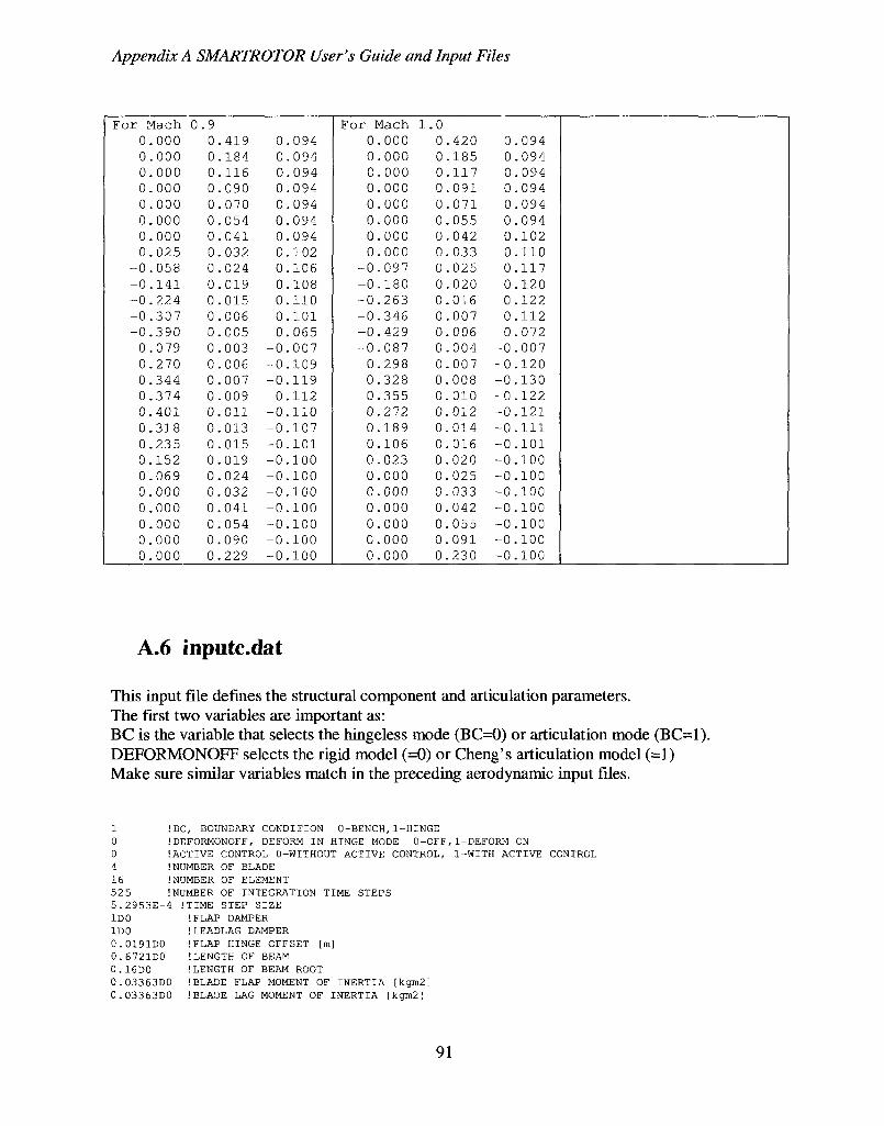
Appendix A SMARTROTOR User's Guide and Input Files
F o r Mach 0 . 0 0 0 0 . 0 0 0 0 . 0 0 0 0 . 0 0 0 0 . 0 0 0 0 . 0 0 0 0 . 0 0 0 0 . 0 2 5
- 0 . 0 5 8 - 0 . 1 4 1 - 0 . 2 2 4 - 0 . 3 0 7 - 0 . 3 9 0 - 0 . 0 7 9
0 . 2 7 0 0 . 3 4 4 0 . 3 7 4 0 . 4 0 1 0 . 3 1 8 0 . 2 3 5 0 . 1 5 2 0 . 0 6 9 0 . 0 0 0 0 . 0 0 0 0 . 0 0 0 0 . 0 0 0 0 . 0 0 0
0 . 9 0 . 4 1 9 0 . 1 8 4 0 . 1 1 6 0 . 0 9 0 0 . 0 7 0 0 . 0 5 4 0 . 0 4 1 0 . 0 3 2 0 . 0 2 4 0 . 0 1 9 0 . 0 1 5 0 . 0 0 6 0 . 0 0 5 0 . 0 0 3 0 . 0 0 6 0 . 0 0 7 0 . 0 0 9 0 . 0 1 1 0 . 0 1 3 0 . 0 1 5 0 . 0 1 9 0 . 0 2 4 0 . 0 3 2 0 . 0 4 1 0 . 0 5 4 0 . 0 9 0 0 . 2 2 9
0 . 0 9 4 0 . 0 9 4 0 . 0 9 4 0 . 0 9 4 0 . 0 9 4 0 . 0 9 4 0 . 0 9 4 0 . 1 0 2 0 . 1 0 6 0 . 1 0 8 0 . 1 1 0 0 . 1 0 1 0 . 0 6 5
- 0 . 0 0 7 - 0 . 1 0 9 - 0 . 1 1 9 - 0 . 1 1 2 - 0 . 1 1 0 - 0 . 1 0 7 - 0 . 1 0 1 - 0 . 1 0 0 - 0 . 1 0 0 - 0 . 1 0 0 - 0 . 1 0 0 - 0 . 1 0 0 - 0 . 1 0 0 - 0 . 1 0 0
F o r Mach 0 . 0 0 0 0 . 0 0 0 0 . 0 0 0 0 . 0 0 0 0 . 0 0 0 0 . 0 0 0 0 . 0 0 0 0 . 0 0 0
- 0 . 0 9 7 - 0 . 1 8 0 - 0 . 2 6 3 - 0 . 3 4 6 - 0 . 4 2 9 - 0 . 0 8 7
0 . 2 9 8 0 . 3 2 8 0 . 3 5 5 0 . 2 7 2 0 . 1 8 9 0 . 1 0 6 0 . 0 2 3 0 . 0 0 0 0 . 0 0 0 0 . 0 0 0 0 . 0 0 0 0 . 0 0 0 0 . 0 0 0
1 .0 0 . 4 2 0 0 . 1 8 5 0 . 1 1 7 0 . 0 9 1 0 . 0 7 1 0 . 0 5 5 0 . 0 4 2 0 . 0 3 3 0 . 0 2 5 0 . 0 2 0 0 . 0 1 6 0 . 0 0 7 0 . 0 0 6 0 . 0 0 4 0 . 0 0 7 0 . 0 0 8 0 . 0 1 0 0 . 0 1 2 0 . 0 1 4 0 . 0 1 6 0 . 0 2 0 0 . 0 2 5 0 . 0 3 3 0 . 0 4 2 0 . 0 5 5 0 . 0 9 1 0 . 2 3 0
0 . 0 9 4 0 . 0 9 4 0 . 0 9 4 0 . 0 9 4 0 . 0 9 4 0 . 0 9 4 0 . 1 0 2 0 . 1 1 0 0 . 1 1 7 0 . 1 2 0 0 . 1 2 2 0 . 1 1 2 0 . 0 7 2
- 0 . 0 0 7 - 0 . 1 2 0 - 0 . 1 3 0 - 0 . 1 2 2 - 0 . 1 2 1 - 0 . 1 1 1 - 0 . 1 0 1 - 0 . 1 0 0 - 0 . 1 0 0 - 0 . 1 0 0 - 0 . 1 0 0 - 0 . 1 0 0 - 0 . 1 0 0 - 0 . 1 0 0
A.6 inputc.dat
This input file defines the structural component and articulation parameters. The first two variables are important as: BC is the variable that selects the hingeless mode (BC=0) or articulation mode (BC=1). DEFORMONOFF selects the rigid model (=0) or Cheng's articulation model (=1) Make sure similar variables match in the preceding aerodynamic input files.
1 !BC, BOUNDARY CONDITION 0-BENCH,1-HINGE 0 !DEFORMONOFF, DEFORM IN HINGE MODE 0-OFF,1-DEFORM ON 0 !ACTIVE CONTROL 0-WITHOUT ACTIVE CONTROL, 1-WITH ACTIVE CONTROL 4 !NUMBER OF BLADE 16 !NUMBER OF ELEMENT 525 iNUMBER OF INTEGRATION TIME STEPS 5.2953E-4 !TIME STEP SIZE 1D0 !FLAP DAMPER ID0 iLEADLAG DAMPER 0.0191D0 !FLAP HINGE OFFSET [m] 0.6721D0 ILENGTH OF BEAM 0.16DO ILENGTH OF BEAM ROOT 0.03363D0 1BLADE FLAP MOMENT OF INERTIA [kgm2] 0.03363D0 !BLADE LAG MOMENT OF INERTIA [kgm2]
91
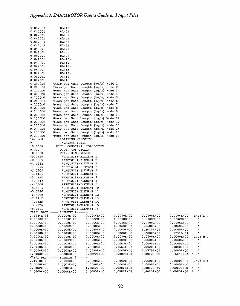
Appendix A SMARTROTOR User's Guide and Input Files
0.042001 0.042001 0.042001 0.042001 0.042001 0.042001 0.042001 0.042001 0.042001 0.042001 0.042001 0.042001 0.042001 0.042001 0.042001 0.042001 0.2000DO 0.2000DO 0.2000D0 0.2000D0 0.2000D0 0.2000D0 0.2000DO 0.2000D0 0.2000D0 0.2000DO 0.2000DO 0.2000D0 0.2000D0 0.2O0OD0 0.2000D0 0.2000D0 164.8d0 0 19.36D0 0.0D0 -0.73D0 -0.2856 -0.8569 -1.4282 -1.9995 -2 5708 -3.1421 -3.7134 -4.2847 -4.8560 -5.4273 -5.9986 -6.5699 -7.1412 -7.7125 -8.2838 -8.8551 MAT'L DATA — 2.1910E-08 O.OOOOE+OO 0.0O00E+O0 0.00O0E+O0 O.OOOOE+OO O.OOOOE+00 5.0000E+00 O.OOOOE+OO O.OOOOE+00 O.OOOOE+00 O.OOOOE+OO O.OOOOE+00 MAT'L DATA — 2.1910E-08 O.OOOOE+OO O.OOOOE+00 O.OOOOE+OO
'DL(l) 'DL(2) 'DL(3) 'DL(4> 'DL(5) 'DL(6) 'DL(7) 1DL(8) 'DL<9) 'DL(IO) 'DL(ll) 'DL(12) 'DL(13) 'DL(14) 'DL(15) 'DL(16)
Mass per Unit Mass per Unit Mass per Unit Mass per Unit Mass per Unit Mass per Unit Mass per Unit Mass per Unit Mass per Unit Mass per Unit Mass per Unit Mass per Unit Mass per Unit Mass per Unit Mass per Unit Mass per Unit
Length Length Length Length Length Length Length Length Length Length Length Length Length Length Length Length
'ROTATING VELOCITY 1 INCREASE SPEED
[kg/m] [kg/m] [kg/m] [kg/m] [kg/m] [kg/m] [kg/m] [kg/m] [kg/m] [kg/m] [kg/m] [kg/m] [kg/m] [kg/m] [kg/m] [kg/m]
'PITCH CONSTANT, COLLECTIVE 'PCOS, COS CYCLIC 'PSIN, SIN CYCLIC 'PRETWIST-'PRETWIST-'PRETWIST-'PRETWIST-I PRE TWIST-'PRETWIST-'PRETWIST-'PRETWIST-'PRETWIST-'PRETWIST-'PRETWIST-'PRETWIST-'PRETWIST-'PRETWIST-'PRETWIST-'PRETWIST-
-— ELEMENT 1 — 0.0000E+00 1.0000E-20 O.OOOOE+00 O.OOOOE+00 O.00OOE+O0 O.OOOOE+00 O.OOOOE+00 5.0000E+00 O.00O0E+00 0.0000E+00 0.0000E+00 O.OOOOE+00
— ELEMENT 2--0.OOO0E+00 1.0000E-20 0.00O0E+O0 O.OOOOE+00
-ELEMENT -ELEMENT -ELEMENT -ELEMENT -ELEMENT -ELEMENT -ELEMENT -ELEMENT -ELEMENT -ELEMENT -ELEMENT -ELEMENT -ELEMENT -ELEMENT -ELEMENT -ELEMENT
1 2 3 4 5 6 7 8 9 10 11 12 13 14 15 16
0.0000E+00 0.O000E+0O 1.0000E-20 0.0000E+00 0.0000E+00 O.OOOOE+00 0.O000E+0O 0.0000E+00 5.0000E+00 0.0000E+00 0.0000E+00 O.OOOOE+00
0.0000E+00 O.OOOOE+00 1.0000E-20 O.OOOOE+00
Node 1 Node 2 Node 3 Node 4 Node 5 Node 6 Node 7 Node 8 Node 9 Node 10 Node 11 Node 12 Node 13 Node 14 Node 15 Node 16
0.0000E+00 0.000OE+0O 0.0000E+00 4.0000E-03 0.0000E+00 0.0000E+00 0.0000E+00 0.0000E+00 0.0000E+00 2.1664E+03 0.0000E+00 0.0000E+00
0.0000E+00 0.0000E+00 0.0000E+00 4.0000E-03
0 0 0 0 5 0 0 0 0 0 1 0
0 0 0 0
0000E+00 O000E+OO 00O0E+OO 0000E+00 2630E-03 0000E+00 0000E+OO 0000E+O0 0000E+O0 0O00E+O0 1779E+05 0000E+00
0000E+0O 00O0E+O0 0000E+00 00OOE+O0
0 0 0 0 0 2 0 0 0 0 0 2
0 0 0 0
0O0OE+00 'inv([K]) 0000E+00 ' " 0000E+00 ' " 0000E+00 ' " OOOOE+00 ' " 1231E-04 ' " 0000E+00 'inv([M]) 0000E+00 ' " 0O00E+0O ' " 0000E+00 ' " 0000E+00 ' 1664E+03 ' "
0000E+0O 'inv([K]) 0000E+00 ' " 0000E+00 ' 0000E+00 ' "
92
Appendix A SMARTROTOR User's Guide and Input Files
O.OOOOE+OO 0.0000E+00 0.0000E+00 0.0000E+00 5.2630E-03 O.OOOOE+00 0.O00OE+00 0.0000E+00 O.OOOOE+00 0.0000E+00 0.0000E+00 2.1231E-04 5.0000E+00 O.OOOOE+00 O.OOOOE+OO O.OOOOE+OO 0.0000E+00 O.OOOOE+OO O.OOOOE+00 5.0000E+00 O.OOOOE+00 O.OOOOE+00 O.OOOOE+00 O.OOOOE+00 O.OOOOE+OO O.OOOOE+00 5.0000E+00 O.OOOOE+00 O.OOOOE+OO O.OOOOE+OO O.OOOOE+00 O.OOOOE+OO O.OOOOE+00 2.1664E+03 O.OOOOE+OO O.OOOOE+OO O.OOOOE+OO O.OOOOE+OO O.OOOOE+OO O.OOOOE+OO 1.1779E+05 O.OOOOE+OO O.OOOOE+OO O.OOOOE+OO O.OOOOE+OO O.OOOOE+OO O.OOOOE+OO 2.1664E+03
The MAT'L DATA — ELEMENT #- repeats up to node 16. These are the inverted stiffness and mass matricies only used for the Opoku/Cheng's hingeless model, and not for the rigid model.
93
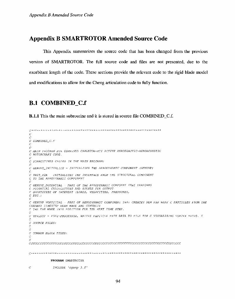
Appendix B Amended Source Code
Appendix B SMARTROTOR Amended Source Code
This Appendix summarizes the source code that has been changed from the previous
version of SMARTROTOR. The full source code and files are not presented, due to the
exorbitant length of the code. These sections provide the relevant code to the rigid blade model
and modifications to allow for the Cheng articulation code to fully function.
B.l COMBINED_C.f
B.l.l This the main subroutine and it is stored in source file COMBINED_C.f.
c c C COMBINED_C.F C C C MAIN PROGRAM FOR COMBINED CARLETON-MIT ACTIVE AEROELASTIC-AEROACOUSTIC C ROTORCRAFT CODE. C C SUBROUTINES CALLED IN THE MAIN PROGRAM: C C GENUVP_INITIALIZE - INITIALIZES THE AERODYNAMIC COMPONENT (GENUVP) C C INIT_S2A - INITIALIZES THE INTERFACE FROM THE STRUCTURAL COMPONENT C TO THE AERODYNAMIC COMPONENT C C GENUVP_POTENTIAL - PART OF THE AERODYNAMIC COMPOENT THAT PERFORMS C POTENTIAL CALCULATIONS AND SOLVES FOR OUTPUT C QUANTITIES OF INTEREST (LOADS, VELOCITIES, PRESSURES, C ETC.) C C GENUVP_VORTICIAL - PART OF AERODYNAMIC COMPONENT THAT CREATES NEW FAR WAKE C PARTICLES FROM THE CURRENT TIMESTEP NEAR WAKE AND CONVECTS C THE FAR WAKE INTO POSITION FOR THE NEXT TIME STEP. C C VPVISTP - POST-PROCESSOR. WRITES PARTICLE PATH DATA TO FILE FOR C VISUALIZING VORTEX PATHS. C C C SOURCE FILES: C C C COMMON BLOCK FILES: C C CCCCCCCCCCCCCCCCCCCCCCCCCCCCCCCCCCCCCCCCCCCCCCCCCCCCCCCCCCCCCCCCCCCCCCCCCCCCCCCCCCC
PROGRAM SMARTROTOR
C INCLUDE 'cgnvp-3.f
94
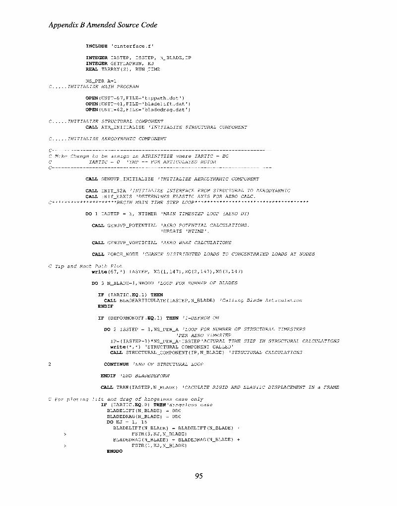
Appendix B Amended Source Code
INCLUDE *cinterface.f'
INTEGER IASTEP, ISSTEP, N_BLADE,IP INTEGER GETFLAPRUN, KJ REAL TARRAY(2), RUN_TIME
NS_PER_A=1 C INITIALIZE MAIN PROGRAM
OPEN(UNIT=6 7,FILE='tippath.dat') OPEN(UNIT=41,FILE='bladelift.dat') OPEN(UNIT=42,FILE='bladedrag.dat')
C INITIALIZE STRUCTURAL COMPONENT CALL ATR_INITIALIZE 'INITIALIZE STRUCTURAL COMPONENT
C INITIALIZE AERODYNAMIC COMPONENT
c C Mike Change to be assign m ATRINITIZE where IARTIC = BC C IARTIC = 0 'IMP — FOR ARTICULATED ROTOR
c
CALL GENUVP_INITIALIZE 'INITIALIZE AERODYNAMIC COMPONENT
CALL INIT_S2A ' INITIALIZE INTERFACE FROM STRUCTURAL TO AERODYANMIC CALL INIT_EAXIS 'DETERMINES ELASTIC AXIS FOR AERO CALC.
C*********************BEGIN MAIN TIME STEP LOOP*************************************
DO 1 IASTEP = 1, NTIMER 'MAIN TIMESTEP LOOP (AERO DT)
CALL GENUVP_POTENTIAL 'AERO POTENTIAL CALCULATIONS. 'UPDATE 'NTIME'.
CALL GENUVP_VORTICIAL 'AERO WAKE CALCULATIONS
CALL F0RCE_NODE 'CHANGE DISTRIBUTED LOADS TO CONCENTRATED LOADS AT NODES
C Tip and Root Path Plot write(67,*) IASTEP, XG(1,147),XG(2,147),XG(3,147)
DO 3 N_BLADE=1,NB0DD 'LOOP FOR NUMBER OF BLADES
IF (IARTIC.EQ.1) THEN CALL BLADEARTICULATE(IASTEP,N_BLADE) 'Calling Blade Articulation
ENDIF
IF (DEFORMONOFF.EQ.l) THEN 'l=DEFROM ON
DO 2 ISSTEP = 1,NS_PER_A 'LOOP FOR NUMBER OF STRUCTURAL TIMESTEPS 'PER AERO TIMESTEP
IP=(IASTEP-1)*NS_PER_A+ISSTEP 'ACTURAL TIME STEP IN STRUCTURAL CALCULATIONS write(*,*) 'STRUCTURAL COMPONENT CALLED' CALL STRUCTURAL_COMPONENT(IP,N_BLADE) 'STRUCTURAL CALCULATIONS
2 CONTINUE 'END OF STRUCTURAL LOOP
ENDIF 'END BLADEDEFORM
CALL TRAN(IASTEP,N_BLADE) 'CACULATE RIGID AND ELASTIC DISPLACEMENT IN a FRAME
C For plotmg lift and drag of hmgeless case only IF (IARTIC.EQ.O) THEN 'Hmgeless case BLADELIFT(N_BLADE) = ODD BLADEDRAG(N_BLADE) = 0D0 DO KJ = 1, 16
BLADELIFT(N_BLADE) = BLADELIFT(N_BLADE) + > FSTR(3,KJ,N_BLADE)
BLADEDRAG(N_BLADE) = BLADEDRAG(N_BLADE) + > FSTR(1,KJ,N_BLADE)
ENDDO
95
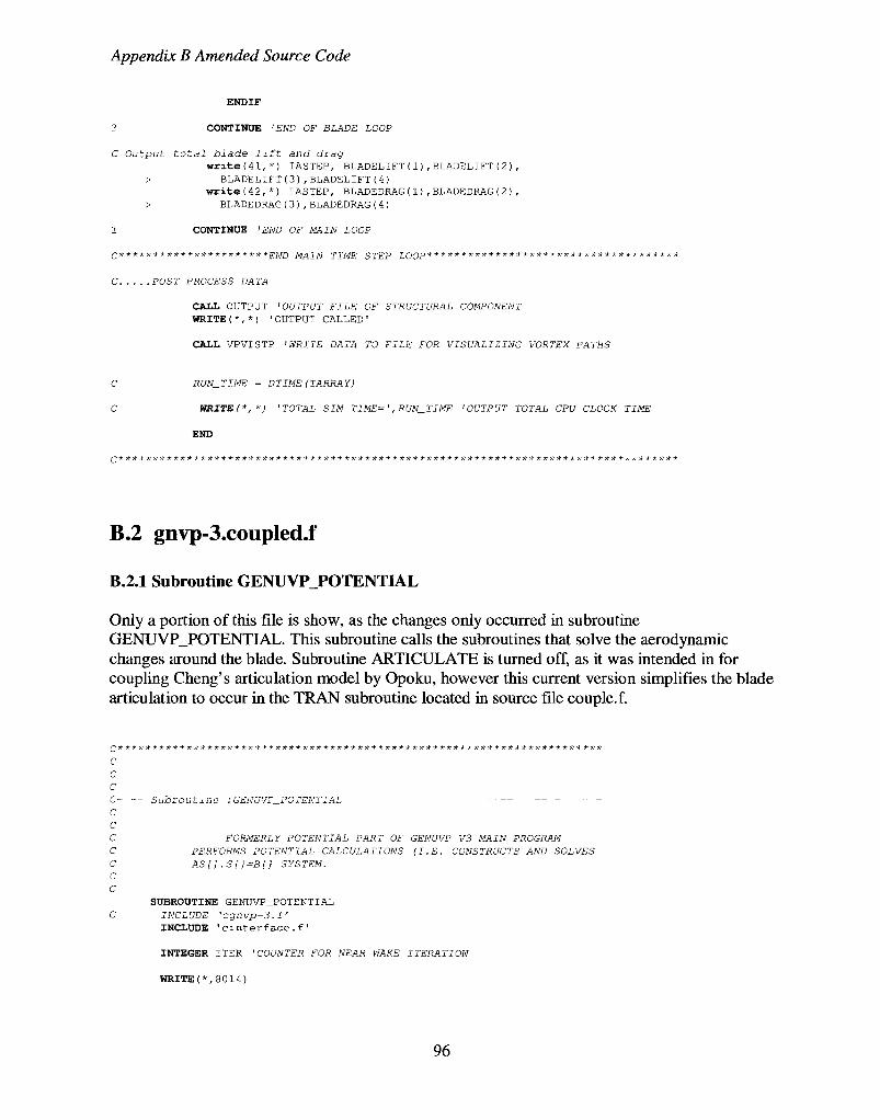
Appendix B Amended Source Code
ENDIF
3 CONTINUE 'END OF BLADE LOOP
C Output total blade lift and drag
write(41,*) IASTEP, BLADELIFT(1),BLADELIFT(2), > BLADELIFT(3),BLADELIFT(4)
write(42,*) IASTEP, BLADEDRAG(1),BLADEDRAG(2),
> BLADEDRAG(3),BLADEDRAG(4)
1 CONTINUE 'END OF MAIN LOOP
C**********************Eiii) MAIN TIME STEP LOOP*************************************
C POST PROCESS DATA
CALL OUTPUT 'OUTPUT FILE OF STRUCTURAL COMPONENT WRITE!* ,*) 'OUTPUT CALLED'
CALL VPVISTP 'WRITE DATA TO FILE FOR VISUALIZING VORTEX PATHS
C RUN_TIME = DTIME(TARRAY)
C WRITE (*,*) 'TOTAL SIM T1ME= ', RUN_TIME 'OUTPUT TOTAL CPU CLOCK TIME
END
B.2 gnvp-3.coupled.f
B.2.1 Subroutine GENUVP_POTENTIAL
Only a portion of this file is show, as the changes only occurred in subroutine GENUVP_POTENTIAL. This subroutine calls the subroutines that solve the aerodynamic changes around the blade. Subroutine ARTICULATE is turned off, as it was intended in for coupling Cheng's articulation model by Opoku, however this current version simplifies the blade articulation to occur in the TRAN subroutine located in source file couple, f.
c
c C - — Subroutj.no : GENUVr_POTENTIAL — - — -C C C FORMERLY POTENTIAL PART OF GENUVP V3 MAIN PROGRAM C PERFORMS POTENTIAL CALCULATIONS (I.E. CONSTRUCTS AND SOLVES C AS[] .S{}=B(} SYSTEM. C C
SUBROUTINE GENUVP_POTENTIAL C INCLUDE 'cgnvp-3.f
INCLUDE 'C3 tit erf ace. f
INTEGER ITER 'COUNTER FOR NEAR WAKE ITERATION
WRITE(*,8014)
96
Appendix B Amended Source Code
c C + AERODYNAMIC COMPONENT TIME STEPS + + + •* + C
2000 NTIME = NTIME + 1 if (NTIME.gt.NTIMER) THEN
WRITE (*,*) 'NTIMER has been reached ...<AERO-COMP-POTEN>' RETURN
END IF
TTIME = TTIME + DT write (* ,8001) NTIME write (IFILEOG,8001) NTIME
C- Part B THE POTENTIAL PART C C C B.l: Fulfill the boundary and emission conditions C C a. Initialize the proccedure C
C DETERMINE THE INFLOW CONDITIONS write (*,8002) call INFLOW
C APPLY ELASTIC DEFORMATION TO THE BLADE CALL BLADE_DEFORM CALL ELAST_BC
C MIKE, ARTICULATE SUBROUTINE SILENCE AS NOT NEEDED, AS CHANGES WERE MADE C IN TRAN subroutine, located m couple.f C MOVE BODIES TO NEXT POSITION C CALL ARTICULATE
write (*,8003) c a l l MOVEBOD
C IF NON-SUBGRID, UPDATE AS [] MATRIX IF REQUIRED write (*,8004) if (IYNSG.eq.0) call MATRIXC
C CALCULATE NORMAL FLOW BOUNDARY CONDITION VECTOR B{) write (*,8005) call BOONDC0
C START POTENTIAL ITERATIONS FOR NEAR WAKE GEOMETRY ITER = 0
C b. Start iterations to define the near-wake contribution C
21 ITER = ITER + 1 C C - Complete the boundary conditions C
write(*,*) 'ITER= * ,ITER
call BOUNDC1 (ITER)
C C - Solve the kinematic part C
if (IYNSG.eq.0) then call POTENTC (ITER)
else call GAOSS_SEIDEL(40,0.0001,itr,err) write(*,*)'GAUSS_SEIDEL ',itr,err
C wot ready for thick endif
97
Appendix B Amended Source Code
if (ITER.eq.l) go to 23 C C CHECK FOR CONVERGENCE
call CONVERG (ITER,ICHECK) C CONVERGECE ACHIEVED
if (ICHECK.eq.l) go to 22
C CONVERGENCE NOT ACHIEVED - PREPARE FOR NEXT ITERATION C * Calculate the emission velocities C 23 IVEMISC = 2
if ( (RELAXU.eq.l.).or.(ITER.eq.l) ) IVEMISC=1 call VEMISC ( IVEMISC )
RELAXF = RELAXU if (IVEMISC.eq.l) RELAXF = 1.
C REDEFINE NEAR WAKE GEOMETRY AND PANELLING call CORRECW (RELAXF)
C * Correct the singularity approximation C
do 24 I=1,NDFT 24 PRES(I) = RELAXS*S(I) + (1.-RELAXS)*PRES(I)
go to 21 C C ***** END OF POTENTIAL ITERATIONS ***** C 22 continue
C CALCULATE DIPOLE ELEMENT INTENSITIES call CONCLUD
C READY FOR C write (*,8010) C
C C B.2: Calculate the force and velocity distribution on the bodies C C
C CALCULATE LOADS, VELOCITIES, PRESSURES, ETC. call RESCPV
C WRITE LOADS AND VISUALIZATION DATA TO FILE CALL WRTCPVTP CALL TPANIM
C CALL ACOUSTIC COMPONENT CALL ACOUSTIC_DATA
C C B.3: TIME DEPENDENT APPLICATION 'FORMER CALL TO ELASTIC CODE C
C call APPLICT
C END OF AERODYNAMIC POTENTIAL CALCULATIONS C CONTINUE WITH VORTICIAL CALCULATIONS AND STRUCTURAL CALCULATIONS
RETURN
8001 format ( // ' '/ ' Time step NTIME = ',i3,4x,'has started'/ . . )
8002 format ( 8003 format ( 8 004 format ( 8 005 format ( 8006 format ( 8007 format (
INFLOW called ' ) MOVEBOD called ' ) MATRIXC called ' ) BOUNDC0 called ' ) ITER=',i2,2x, ' BOUNDC1 called' )
POTENTC called' )
98
Appendix B Amended Source Code
8009 format ( ' CORRECW called' ) 8010 format ( /' Succesful termination of time step'/
. . ) 8011 format ( ' RESCPV called' ) 8012 format ( ' CREATE called' ) 8013 format ( ' DEFORM called' ) 8014 format ( ' GENUVP_POTENTIAL called' )
C C 9999 format (3el4.5) 1234 format (I4,13el5.5)
END
B.3 blade deform.f
B.3.1 Subroutine BLADE DEFORM
This subroutine was changed to call TWIST 123 to allow for full articulated displacement of the aerodynamic grid nodes.
************
C PART 2/4: BLADE ELASTIC DEFORMATION C — » APPLIES STRUCTURAL FEEDBACK TO DEFORM AERODYNAMIC BODIES
C C Subroutine :BLADE_DEFORM C C C APPLIES ELASTIC DEFORMATION TO BLADE MESH BASED ON FEEDBACK FROM C STRUCTURAL CODE. C C
SUBROUTINE BLADE_DEFORM INCLUDE 'cinterfacp.f'
REAL DIS_1, DIS_2, DIS_3, TORS_ANG INTEGER K, N, NB, ISECT, ICHORD, NBA, ND
REALXI(J), XF(3), R_AXIS(o)
C Articulated Variables REAL TORS_X, TORS_Y, TORS_Z
W R I T E ( * , 8 0 1 3 )
ITIALIZE SUBROUTINE DIS 1 = 0 . DIS 2 = 0 . DIS 3 = 0 . TORS_ANG =
DO K = l , 3 XI XF
E0 E0 E0
= 0 . E 0
(K) (K)
VARIABLES
0 : 0
.E0
.E0
99
Appendix B Amended Source Code
R_AXIS(K) = O.EO ENDDO
C INITIALIZE SUBROUTINE (STORE LOCAL COORDINATES AND FIND ELASTIC AXIS VECTOR C FOR EACH NODE)
IF (I_BLD_DEFORM.NE.l) THEN 'First Call of Blade Deform
DO N=1,NNT 'STORE UNDEFORMED LOCAL GEOMETRY
XGL_RIGID(1,N) = XGL(1,N) XGL_RIGID(2,N) = XGL(2,N) XGL_RIGID(3,N) = XGL(3,N)
ENDDO
DO 1 NB=l,NBODELT 'FOR EACH ELASTIC BODY NBA = NBODA(NB) 'AERO BODY NUMBER
DO 11 ISECT = 1,NCWB(NBA) 'SPANWISE NODAL SECTION DO 12 ICHORD = 1,NNBB(NBA) 'CHORDWISE NODAL SECTION
'NODE NUMBER 'ND' ND = NNTBACC(NBA-l) + (ISECT-1)*NNBB(NBA) + ICHORD 'VECTOR FROM SECTION ELASTIC AXIS POINT TO NODE • ND ' R_E_AXIS(1,ND)= XGL_RIGID(1,ND) - E_AXIS(1,NBA,ISECT) R_E_AXIS(2,ND)= XGL_RIGID(2,ND) - E_AXIS(2,NBA,ISECT) R_E_AXIS(3,ND)= XGL_RIGID(3,ND) - E_AXIS(3,NBA,ISECT)
12 CONTINUE
11 CONTINUE
1 CONTINUE
I_BLD_DEFORM = 1
ENDIF
C USE LINEAR INTERPOLATION TO MAP ELASTIC DEFORMATION
C TO AERODYNAMIC SPANWISE NODAL SECTIONS
CALL MAP_DEFORM
C APPLY ELASTIC DEFORMATION TO EACH ELASTIC BODY
DO 2 NB=l,NBODELT 'LOOP FOR EACH ELASTIC BODY NBA = NBODA(NB) 'AERO BODY NUMBER DO 21 ISECT = 1,NCWB(NBA) 'LOOP FOR EACH SPANWISE NODAL SECTION
DO 22 ICHORD = 1,NNBB(NBA) 'CHORDWISE NODAL SECTION
'NODE NUMBER 'ND' ND = NNTBACC(NBA-l) + (ISECT-1)*NNBB(NBA) + ICHORD
DO K=I,3 XI (K) = XGL_RIGID(K,ND) XF (K) = O.EO R_AXIS(K) = R_E_AXIS(K,ND)
ENDDO IF (IARTIC.EQ.O) THEN 'Hmgeless
'CALCULATE ELASTIC TORSIONAL TWIST TORS_ANG = TWIST_2 (NTIME, NBA, ISECT) 'MUST BE IN RADIANS CALL TWISTPT(2,TORS_ANG,R_AXIS, XI, XF)
ELSE 'Articulated Version TORS_X = TWIST_1(NTIME,NBA, ISECT) 'MUST BE IN RADIANS TORS_Y = TWIST_2(NTIME,NBA,ISECT) 'MUST BE IN RADIANS TORS_Z = TWIST_3 (NTIME, NBA, ISECT) 'MUST BE IN RADIANS CALL TWIST123(TORS_X,TORS_Y,TORS_Z,R_AXIS,XI,XF)
100
Appendix B Amended Source Code
ENDIF
•APPLY ELASTIC TORSIONAL TWIST DO K=l,3
XGL (K,ND) = XF(K) ENDDO
'.ELASTIC DISPLACEMENT DIS_1 = DISP_1(NTIME,NBA,ISECT) DIS_2 = DISP_2(NTIME,NBA,ISECT) DIS_3 = DISP_3(NTIME,NBA,ISECT)
'.APPLY ELASTIC DISPLACEMENT XGL (1,ND) = XGL(1,ND) + DIS_1 XGL (2,ND) = XGL(2,ND) + DIS_2 XGL (3,ND) = XGL(3,ND) + DIS_3
C Mike XGL Check Last Span node, chord nodes IF (ISECT.EQ.NCWB(NBA)) THEN write(*,*) 'XGL + DIS', NBA, ND, XGL(1,ND),XGL(2, ND) , XGL(3,ND)
ENDIF
22 CONTINUE ! END CHORDWISE NODAL SECTION LOOP
21 CONTINUE .'END SPANWISE NOCAL SECTION LOOP
2 CONTINUE '.END ELASTIC BODY LOOP
C RECALCULATE BODY PANEL GEOMETRY DATA IN LOCAL COORDINATES
CALL GBEMBODL_MOD
RETURN
8013 format ( ' BLADE_DEFORM called' )
END
B.3.2 Subroutine TWISTPT
This is the unchanged subroutine that rotates the aerodynamic chordwise nodes only pitchwise in the hingeless mode.
C Subroutine : TWISTPT C C C BASED ON ROTATEP (LIBRAR-3. F) . ROTATES XINIT (3), AT A RADIUS OF C RAXIS (3) FROM THE ELASTIC AXIS, THROUGH ANGLE THETA_ANG C (RADIANS). RETURNS XFINAL(3). C C C
SUBROUTINE TWISTPT (I_AXIS, THETA_ANG, RAXIS, XINIT, XFINAL)
IMPLICIT NONE
REAL COSTH, SINTH, THETA_ANG, RAXIS REAL XINIT, XFINAL, DELTAX, XROTATE
dimension XINIT(3), XFINAL(3) dimension XROTATE(3), DELTAX(3), RAXIS(3)
INTEGER I_AXIS
C COS & SIN OF TWIST ANGLE
101
Appendix B Amended Source Code
COSTH = COS (THETA_ANG) SINTH = SIN (THETA_ANG)
go to (1,2,3), I_AXIS
C Rotation about X axis - CROSS SECTION WARPING
1 WRITE(*,*) 'Rotation about XI not defined in TWISTPT'
XFINAL(1) = XINIT(1) XFINAL(2) = XINIT(2) XFINAL(3) = XINIT(3)
return
C Rotation about Y axis - CROSS SECTION TWISTING
C ROTATE R_E_AXIS VECTOR 2 XROTATE(l) = RAXIS(1)*COSTH + RAXIS(3)*SINTH
XR0TATE(3) = - RAXIS(1)*SINTH + RAXIS(3)*COSTH C FIND XI & X3 DISPLACEMENTS
DELTAX(l) = XROTATE(l) - RAXIS(1) DELTAX(3) = XR0TATE(3) - RAXIS(3)
C ADD DISPLACEMENTS TO INITIAL COORDINATES XFINAL(1) = XINIT(l) + DELTAX(l) XFINAL(2) = XINIT(2) XFINAL(3) = XINIT(3) + DELTAX(3)
return
C Rotation about Z axis - CROSS SECTION WARPING
3 WRITE(*,*) 'Rotation about X3 not defined in TWISTPT'
XFINAL(1) = XINIT(1) XFINAL(2) = XINIT(2) XFINAL(3) = XINIT(3)
return END
B.3.3 Subroutine TWIST123
This is the subroutine, based from TWISTPT that rotates and displaces the aerodynamic chordwise nodes from the hinge, in the articulation mode.
C Subrout ine .-TWIST123 CMike Added Subroutine C C BASED ON ROBOTICS ROTATION. C RETURNS XFINAL(3). C C C
SUBROUTINE TWIST123 (THETA_X,THETA_Y,THETA_Z,RAXIS,XINIT,XFINAL)
IMPLICIT NONE
REAL THETA_X,THETA_Y,THETA_Z, RAXIS REAL XINIT, XFINAL, DELTAX, XROTATE
dimension XINIT(3), XFINAL(3) dimension XROTATE(3), DELTAX(3), RAXIS(3)
102
Appendix B Amended Source Code
C ROTATE R__E_AXIS VECTOR XROTATE(l) = COS(THETA_Y)*COS(THETA_Z)*RAXIS(1) -
> COS(THETA_Y)*SIN(THETA_Z)*RAXIS(2) + > SIN(THETA_Y)*RAXIS(3)
XROTATE(2) = (SIN(THETA_X)*SIN(THETA_Y)*COS(THETA_Z) + > COS(THETA_X)*SIN(THETA_Z))*RAXIS(1) + > (-SIN(THETA__X) *SIN(THETA_Y) *SIN(THETA_Z) + > COS(THETA_X)*COS(THETA_Z))*RAXIS(2) -> SIN(THETA_X)*COS(THETA_Y)*RAXIS(3)
C (sPitch*sFlap*cLag+cPitch*sLag) *dx+ (~sPitch*sFlap*sLag+cPitch*cLag) *dy-sPitch*cFlap*dz
XROTATEO) = (-COS(THETA_X)*SIN(THETA_Y)*COS(THETA_Z) + > SIN(THETA_X)*SIN(THETA_Z))*RAXIS(1) + > (COS(THETA_X)*SIN(THETA_Y)*SIN(THETA_Z) + > SIN(THETA_X)*COS(THETA_Z))*RAXIS(2) + > COS(THETA_X)*COS(THETA_Y)*RAXIS(3)
C(-cPitch*sFlap*cLag+sPitch*sLag) *dx+ (cPitch*sFlap*sLag+sPitch*cLag) *dy+cPitch*cFlap*dz
C FIND XI & X3 DISPLACEMENTS DELTAX(l) = XROTATE(l) - RAXIS(l) DELTAX(2) = XROTATE(2) - RAXIS(2) DELTAX(3) = XROTATEO) - RAXIS(3)
C ADD DISPLACEMENTS TO INITIAL COORDINATES XFINAL(l) = XINIT(l) + DELTAX(1) XFINAL(2) = XINIT(2) + DELTAX(2) XFINAL(3) = XINIT(3) + DELTAX(3)
return
B.3.4 Subroutine MAP_DEFORM
This subroutine was modified to allow the aerodynamic nodes to be extrapolated and interpolated to their new positions in the articulate mode.
Subroutine :MAP_DEFORM
USES LINEAR INTERPOLATION TO MAP STRUCTURAL DEFORMATION TO AERODYNAMIC MESH.
SUBROUTINE MAP_DEFORM INCLUDE 'cinterface.f'
INTEGER NBA >.AERO BODY NUMBER
INTEGER NBE '.ELASTIC BODY NUMBER INTEGER NDE !ELASTIC NODE NUMBER INTEGER ILAST !LAST ARRAY ELEMENT OF ELASTIC DATA INTEGER K ! COUNTER INTEGER ISECT !COUNTER FOR AERODYNAMIC NODAL SECTION
REAL U_(3,NNTEBM+1) REAL THETA_(3,NNTEBM+1)
!ELASTIC DISPLACEMENT 'ELASTIC ROTATION
. INITIALIZE SUBROUTINE VARIABLES
DO K = 1 , 3 DO L=1,NNTEBM+1
103
Appendix B Amended Source Code
U_(K,L) = 0. THETA_(K,L) = 0.
ENDDO ENDDO
C CONVERT ELASTIC DISPLACEMENTS AND ROTATIONS FROM STRUCTURAL 'a' COORD. SYS.
C TO AERO 'X-LOCAL ' COORD. SYS.
DO 2 NBE=l,NBODELT 'FOR EACH ELASTIC BODY
NBA=NBODA(NBE) 'CORRESPONDING AERO BODY NUMBER
C Mikes Modified Code at 1st node root
'ROOT VALUES. . . .1ST ARRAY ELEMENT IF (IARTIC.EQ.O) THEN 'HINGELESS U_ (1, 1) = 0 . U_ ( 2, 1) = 0 . U_ (3, 1) = 0 . THETA_(1,1) = 0. THEIA_(2,1) = 0 . THETA_(3,1) = 0.
ELSE ' HINGED C Assuming delx equally spaces C Linear extrapolation from DISP nodes 2 & 1 to zero root
U_(l,l) = 2.*(-l.*DISP_2D(NTIME-l,NBA,1)) -> (-l.*DISP_2D(NTIME-l,NBA,2))
U_(2,l) = 2.*(+l.*DISP_lD(NTIME-l,NBA,1)) -> (+1.*DISP_1D(NTIME-1,NBA,2))
U_(3,l) = 2.*(+l.*DISP_3D(NTIME-l,NBA,l)) -> (+1.*DISP_3D(NTIME-1,NBA,2))
THETA_(1,1) = 2.*TWIST_2D(NTIME-1,NBA, 1) -> TWIST_2D(NTIME-1,NBA,2)
THETA_(2,1) = 2.*TWIST_1D(NTIME-1,NBA,1) -> TWIST_1D(NTIME-1, NBA,2)
THETA_(3,1) = 2.*TWIST_3D(NTIME-1,NBA,1) -> TWIST_3D(NTIME-1, NBA,2)
ENDIF 'End of ROOT NODE CASES
'TIP VALUES . . . N_NDSTRB+1 ARRAY ELEMENT ' (I.E. LAST ARRAY ELEMENT) ILAST = N_NDSTRB + 1
IF(NTIME.GT.l) THEN 'FIRST USE OF ELASTIC FEEDBACK
U_(l,ILAST) = -l.*DISP_2DTIP(NTIME-l,NBA) U_(2,ILAST) = +1.*DISP_1DTIP(NTIME-1,NBA) U_(3,ILAST) = +1.*DISP_3DTIP(NTIME-1,NBA) THETA_(1,ILAST) = -1.*TWIST_2DTIP(NTIME-1,NBA) THETA_{2,ILAST) = +i.*TWIST_1DTIP(NTIME-1, NBA) THETA_{3,ILAST) = +1.*TWIST_3DTIP(NTIME-1,NBA)
DO 21 NDE=1,N_NDSTRB -1 'LOOP FOR EACH STR. ELEMENT
U_(1,NDE+1) = -l.*DISP_2D(NTIME-1,NBA,NDE) U_(2,NDE+1) = +1.*DISP_1D(NTIME-1,NBA,NDE) U_(3,NDE+1) = +1.*DISP_3D(NTIME-1,NBA,NDE)
IF (IARTIC.EQ.O) THEN 'HINGELESS THETA_(1,NDE+1) = 0. THETA_(2,NDE+1) = TWIST_1D(NTIME-1,NBA,NDE) THETA_(3,NDE+1) = 0.
ELSE 'Articulated Version: THETA_(1,NDE+1) = -TWIST_2D(NTIME-1,NBA,NDE) THETA_(2,NDE+1) = TWIST_1D(NTIME-1,NBA,NDE) THETA_(3,NDE+1) = TWIST_3D(NTIME-1,NBA,NDE)
ENDIF
21 CONTINUE 'END ELEMENT LOOP
104
Appendix B Amended Source Code
ENDIF 'FIRST USE FO ELASTIC FEEDBACK
DO 23 ISECT=1,NCWB(NBA) 'LOOP FOR EACH AERO SPANWISE •NODAL SECTION
i INDEX AND STORE INTERPOLATED ELASTIC DISPLACEMENTS AND ROTATIONS
IF(ND_STR(ISECT).EQ.l) THEN 'ROOT END NODAL SECTION
DISP_1 (NTIME,NBA,ISECT) = U_(l,l) DISP_2 (NTIME,NBA,ISECT) = U_(2,l) DISP_3 (NTIME,NBA,ISECT) = U_(3,l)
TWIST_1 (NTIME,NBA,ISECT) = THETA_(1,1) TWIST_2 (NTIME,NBA,ISECT) = THETA_(2,1) TWIST_3 (NTIME,NBA,ISECT) = THETA_(3,1)
ELSEIF(ND_STR(ISECT).EQ.N_NDSTRB) THEN 'TIP END NODAL SECTION
DISP_1 (NTIME,NBA,ISECT) = U_(1,ILAST) DISP_2 (NTIME,NBA,ISECT) = U_(2,ILAST) DISP_3 (NTIME,NBA,ISECT) = U_(3,ILAST)
TWIST_1 (NTIME,NBA,ISECT) = THETA_(1,ILAST) TWIST_2 (NTIME,NBA,ISECT) = THETA_(2,ILAST) TWIST_3 (NTIME,NBA,ISECT) = THETA_(3,ILAST)
ELSE ' INTERMEDIATE NODAL SECTIONS
DISP_1(NTIME,NBA,ISECT)= 0.5 * ( U_ (1,ND_STR(ISECT)+1) + U_(1,ND_STR(ISECT)) )
DISP_2(NTIME,NBA,ISECT)= 0.5 * ( U_(2,ND_STR(ISECT)+1) + U_(2,ND_STR(ISECT)) )
DISP_3(NTIME,NBA,ISECT)= 0.5 * ( U_(3,ND_STR(ISECT)+1) + U_(3,ND_STR(ISECT)) )
TWIST_1(NTIME,NBA, ISECT) = 0.5 * ( THETA_(1,ND_STR(ISECT)+1) + THETA_(1,ND_STR(ISECT)) )
TWIST_2(NTIME,NBA,ISECT)= 0.5 * ( THETA_(2, ND_STR(ISECT)+1) + THETA_(2,ND_STR(ISECT)) )
TWIST_3(NTIME,NBA, ISECT)= 0.5 * ( THETA_(3, ND_STR(ISECT)+1)
+ THETA_(3,ND_STR(ISECT)) )
ENDIF
23 CONTINUE 'END AERO SPANWISE NODAL SECTION LOOP
2 CONTINUE 'END ELASTIC BODY LOOP
1121 format (300E12.4)
return END
B.4 bladearticf
B.4.1 Subroutine BLADEARTICULATE
This subroutine is the structural model for the rigid model.
105
Appendix B Amended Source Code
SUBROUTINE BLADEARTICULATE(IASTEP,N_BLADE)
INCLUDE •cATRc.f• INCLUDE 'chinge.f DOUBLE PRECISION YBLADESPAN,MASSMOMSUM,LIFTSUM,DRAGSUM DOUBLE PRECISION GRAVITYACL DOUBLE PRECISION G_FORCE '.Variable Force Parameter INTEGER IASTEP, I,J,N_BLADE
C Ordinary Differential Equation subroutine variables EXTERNAL FEX INTEGER IOPT, ISTATE, ITASK, ITOL, IWORK(20), LIW, LRW, * MF, NEQ DOUBLE PRECISION ATOL(4),RTOL, RWORK(84), TIN, TOUT, Y(4)
LIFTMOMSUM = 0D0 DRAGMOMSUM = 0D0 MASSMOMSUM = 0D0 LIFTSUM = 0D0 DRAGSUM = 0D0 YBLADESPAN = BEAMROOT + DL(1)/2D0 !Y pos at node 1 GRAVITYACL = 9.81D0 !m/s~2
DO I = 1, NES C RECHECK INTEGRAL TO SUM m Excel C RESET UP ACCORDINGLY
LIFTMOMSUM = LIFTMOMSUM + (ARTICLIFT(I,N_BLADE)-> GRAVITYACL*MASSPERUL(I)*DL(I))*(YBLADESPAN-FLAPOFFSET)
DRAGMOMSUM = DRAGMOMSUM + ARTICDRAG(I,N_BLADE)*(YBLADESPAN-> FLAPOFFSET)
MASSMOMSUM = MASSMOMSUM + MASSPERUL(I)*DL(I)*(YBLADESPAN-> FLAPOFFSET)
YBLADESPAN = YBLADESPAN + DL(I)/2D0 + DL(I+1)/2D0 LIFTSUM = LIFTSUM + ARTICLIFT(I,N_BLADE) DRAGSUM = DRAGSUM + ARTICDRAG (I, N_BLADE)
ENDDO UPSILONSQFLAP = IDO + (FLAPOFFSET*MASSMOMSUM)/BLADEIFLAP UPSILONSQLAG = (FLAPOFFSET*MASSMOMSUM)/BLADEILAG
C Write output in COMBINED^C.f BLADELIFT(N_BLADE) = LIFTSUM BLADEDRAG(N_BLADE) = DRAGSUM
IF (IASTEP.EQ.l) THEN C Setting Y to zero as not articulated during the first Timesteps
Y(l) = 0D0 Y(2) = 0D0 Y(3) = 0D0 Y(4) = 0D0
ELSE Y(l) = YFLAPANG(N_BLADE,IASTEP-1) Y(2) = YFLAPVEL(N_BLADE,IASTEP-1) Y(3) = YLLAGANG(N_BLADE,IASTEP-1) Y(4) = YLLAGVEL(N_BLADE,IASTEP-1)
ENDIF
NEQ = 4 ITOL = 1 il sets precision to RTOL ATOL(l) = l.D-9 ATOL(2) = l.D-9 ATOL(3) = l.D-9 ATOL(4) = l.D-9 RTOL = 1D-6 '.Precision Setting
ITASK = 1 !ODE Subroutine Coefficient ISTATE = 1 !ODE Subroutine Coefficient IOPT = 0 '.ODE Subroutine Coefficient
106
Appendix B Amended Source Code
LRW = 84 'Described m ode subroutine instructions LIW = 20 'Described in ode subroutine instructions MF = 10 'Described in ode subroutine instructions TIN = DBLE(IASTEP 1)*DTS TOUT = DBLE(IASTEP)*DTS
write!*,*) 'Tin', TIN, ' TOUT', TOUT, ' DTS', DTS C Additional Input Variables as listed m odemout f C INITIAL VELOCITY
IF (IASTEP LT.IS) THEN DO J=1,NES
0MEGODE=IASTEP*W/IS ' t imestep*OMEGA/INCREASESPEED ENDDO
ELSE DO J=1,NES
OMEGODE = W ENDDO
END IF
ODECOUNT = 0
CALL DLSODE (FEX, NEQ, Y, TIN, TOUT, ITOL, RTOL, ATOL, ITASK, > ISTATE, IOPT, RWORK, LRW, IWORK, LIW, ajm, MF) WRITE(*,*) 'Angles', N_BLADE, IASTEP, (Y(1)*180DO/PiPi), > (Y(2)*180D0/PiPi),(Y(3)*180D0/PiPi),(Y(4)*180D0/PiPi)
C This allocates the flap lag variables per time step YFLAPANG(N_BLADE,IASTEP) = Y(l) 'Flap Angle YFLAPVEL(N_BLADE,IASTEP) = Y(2) 'Flap Angle Velocity YLLAGANG(N_BLADE, IASTEP) = Y(3) 'Lag Angle YLLAGVEL(N_BLADE,IASTEP) = Y(4) 'Lag Angle Velocity
FLAPANGLE(N_BLADE,IASTEP) = YFLAPANG(N_BLADE, IASTEP) LAGANGLE(N_BLADE,IASTEP) = YLLAGANG(N_BLADE,IASTEP)
END 'End of BLADEARTICULATE
B.5 odeblade.f
B.5.1 Subroutine FEX
This subroutine contains the Leishman equations of motions that are solved using the ordinary differential equation solver ODEPACK.
SUBROUTINE FEX (NEQ, T,Y, YDOT) INCLUDE 'chinqe f INTEGER NEQ DOUBLE PRECISION T, Y(4), YDOT(4)
ODECOUNT = ODECOUNT+1 YDOT(1)=Y(2)*FLAPDAMPER YDOT(2)=(LIFTMOMSUM/BLADEIFLAP)-UPSILONSQFLAP* (OMEGODE**2D0) *YU)-> 2D0*OMEGODE*Y(l)*Y(4) YDOT(3)=Y(4)* LEADLAGDAMPER YDOT(4)=(DRAGMOMSUM/BLADEILAG)-UPSIL0NSQLAG*(OMEGODE**2D0)*Y(3)-> 2D0*OMEGODE*Y(l)*Y(2)
ODEFLAPACL = YDOT(2) 'Flap Acceleration Saved ODELLAGACL = YDOT(4) 'Leadlag Acceleration Saved
RETURN END
107

Appendix B Amended Source Code
Subroutines DLSODE, DLSODES, DLSODA, DLSODAR, DLSODPK, DLSODKR, DLSODI, DLSOIBT, DLSODIS omitted for clarity, but located in odeblade.f. Other ODEPAK Subroutines located in files odepack_subl.f and odepack_sub2.f Refer to: Alan Hindmarsh, ODEPACK, a Systematized Collection of ODE Solvers, in Scientific Computing, Elsevier, 1983. Located at Website: http://people.sc.fsu.edu/~jburkardt/f77_src/odepack/odepack.html
B.6 couplcf
B.6.1 Subroutine TRAN
This subroutine contains prepares the displacements and orientations of the structural nodes that were solved in the STRUCTURAL_COMPONENT subroutine. This information is sent to subroutine BLADE_DEFORM, in source code file blade_deform.f, as listed in Appendix B.3.
c C THE INPUT/OUTPUT FILES C C COMMON BLOCKS FILES 'cATRc.f' C ATR_INITIALIZE INITIALIZE ALL THE VARIABLES C STRUCTURAL_C0MPONENT MAIN PROGRAM FOR THE STRUCTURE CODE C equations Caculate Fx C Jacobi Calculate Jacobi matrix C unknows Calculat each variable from vector X C ludcmp2 LU decomposition C lubksb2 Back substitution C t Convert a vector to its dual matrix C ctlyb Calculate transpose of C matrix from theta C CTd Calculate dCT/dt, dP/dt,dH/dt, du/dt,dtheta/dt using C finite difference method C dif Calculate dCTdot/dtheta C mm Multiply of two matrices C mv Multiply of matrix and vector C vv Multiply of two vectors C m_m Plus of two matrices C v__v Plus of two vectors C cross Convert a column vector to its dual matrix C OUTPUT Output unknown variables to different files for plot C
SUBROUTINE TRAN(IASTEP,N_BLADE) C IMPLICIT NONE
INCLUDE 'cATRc.f INTEGER IASTEP,N_BLADE,NELE,I,J,K DOUBLE PRECISION TH_R0DR(3), 'RODRIGUES PARAMETERS
T_0_ANG(3) 'SPACE 1-2-3 ORIENTATION ANGLES
DOUBLE PRECISION PTCANG, FLPANG, LAGANG 'TEMPORARY PITCH, FLAP, LAG ANGLE. DOUBLE PRECISION OMEGEAPITCH 'Temporary OMEGA FOR PITCH CALC DOUBLE PRECISION FIANGLEPITCH 'Temporary FIANGLE FOR PITCH CALC
C Articulate ON & Deform OFF IF(BC.EQ.l.AND.DEFORMONOFF.EQ.O) THEN 'ARTICULATED & Deform Off
108
Appendix B Amended Source Code
IF (IASTEP.EQ.l.AND.N_BLADE.EQ.l) THEN '.OPEN FLAPLAGPLOT OPEN(UNIT=79,FILE='pflangle.dat' ) '.Pitch, Flap, Lag Plot OPEN(UNIT=45,FILE='bdistip.dat') .Tip Path Plot OPEN(UNIT=68,FILE='bladecurve.dat' ) '.Blade Curve Plot
ENDIF C INITIAL VELOCITY
IF (IASTEP.LT.IS) THEN OMEGEAPITCH=IASTEP*W/IS FIANGLEPITCH=0.5*0MEGEAPITCH*(IASTEP*DTS)
ELSE OMEGEAPITCH=W FIANGLEPITCH=0.5*0MEGEAPITCH*(IS*DTS)
$ +OMEGEAPITCH*(IASTEP-IS)*DTS ENDIF
C CACULATE PITCH ANGLE PITCHANGLE(IASTEP, N_BLADE) = (PCON $ +PC0S*C0S(FIANGLEPITCH+N_BLADE*PlPl/2) $ +PSIN*SIN(FIANGLEPITCH+N_BLADE*PiPl/2))*PiPi/180
C Temporarily assign Pitch, Flap and Lag to reduce equation text length PTCANG = PITCHANGLE(IASTEP,N_BLADE) FLPANG = -FLAPANGLE(N_BLADE,IASTEP) LAGANG = -LAGANGLE(N_BLADE,IASTEP)
C Output Pitch, Flap, and Lag Angles IF (N_BLADE.EQ.1) THEN .'Plot only Bladel write(79,*) IASTEP,-FLPANG*180D0/PiPi, LAGANG*180D0/PiPi
ENDIF
write(*,*) 'DEG ANGLES', FLPANG*180D0/PiPi, LAGANG*180DO/PiPi write(*,*) 'FLAPOFFSET', FLAPOFFSET
c
C Changing BEAMROOT to FLAPOFFSET DO NELE=1, NES
C Set Deform DISPLACEMENTS TO Zero For now 'ASSIGN Pitch, Flap/Lag ANGLES
C Pitch Twist Already Taken Into Account in movebod TWIST_1D(IASTEP, N_BLADE,NELE)=0D0 TWIST_2D(IASTEP,N_BLADE,NELE)=-FLAPANGLE(N_BLADE,IASTEP) TWIST_3D(IASTEP,N_BLADE, NELE ) =-LAGANGLE (N_BLADE,IASTEP)
DISP_1D(IASTEP, N_BLADE,NELE) = COS(FLPANG)*COS(LAGANG)* > (RADIUS(NELE)-FLAPOFFSET) + FLAPOFFSET - RADIUS(NELE)
DISP_2D(IASTEP,N_BLADE,NELE) = (SIN(PTCANG)*SIN(FLPANG)* > COS(LAGANG)+COS(PTCANG)*SIN(LAGANG))*(RADIUS(NELE)-FLAPOFFSET)
DISP_3D(IASTEP,N_BLADE,NELE) = (-COS(PTCANG)*SIN(FLPANG)* > COS(LAGANG)+SIN(PTCANG)*SIN(LAGANG))*(RADIUS(NELE)-FLAPOFFSET)
writef*,*) 'DISP', N_BLADE, NELE, DISP_1D(IASTEP,N_BLADE,NELE), > DISP_2D(IASTEP,N_BLADE,NELE), DISP_3D(IASTEP,N_BLADE,NELE)
ENDDO !End spanwise nodes NES
DISP_1DTIP(IASTEP,N_BLADE) = COS(FLPANG)*COS(LAGANG)* > (RADIUS(NES+i)-FLAPOFFSET) + FLAPOFFSET - RADIUS(NES+1)
DISP_2DTIP(IASTEP,N_BLADE) = (SIN(PTCANG)*SIN(FLPANG)* > COS(LAGANG)+COS(PTCANG)*SIN(LAGANG))*(RADIUS(NES+1)-FLAPOFFSET)
DISP_3DTIP(IASTEP,N_BLADE) = (-COS(PTCANG)*SIN(FLPANG)* > COS(LAGANG)+SIN(PTCANG)*SIN(LAGANG))*(RADIUS(NES+1)-FLAPOFFSET)
C Plot Total Tip Path IF (N_BLADE.EQ.l) THEN write(45,*) IASTEP, DISP_1DTIP(IASTEP,N_BLADE),
> DISP_2DTIP(IASTEP,N_BLADE),DISP_3DTIP(IASTEP,N_BLADE) write(68,*) IASTEP,' X ',
109
Appendix B Amended Source Code
> DISP_1D(lASTEP,1,1),DISP_1D(lASTEP,1,2) , > DISP_1D(IASTEP,1,3),DISP_1D(lASTEP,1,4),DISP_1D(lASTEP,1,5), > DISP_1D(IASTEP,1,6),DISP_1D(lASTEP,1,7) ,DISP_1D(lASTEP, 1,8), > DISP_1D(lASTEP,1,9),DISP_1D(lASTEP,1,10),DISP_1D(lASTEP,1,11), > DISP_1D(lASTEP,1,12) ,DISP_1D(lASTEP,1,13),DISP_1D(lASTEP, 1, 14) , > DISP_1D(lASTEP,1,15),DISP_1D(lASTEP,1,16),DISP_1DTIP(lASTEP,1)
write(68,*) lASTEP,' Y ', > DISP_2D(lASTEP,1,1),DISP_2D(lASTEP,1,2), > DISP_2D(lASTEP,1,3),DISP_2D(lASTEP,1,4),DISP_2D(lASTEP, 1, 5) , > DISP_2D(lASTEP,1,6),DISP_2D(lASTEP,1,7),DISP_2D(lASTEP,1,8), > DISP_2D(lASTEP,1,9),DISP_2D(lASTEP,1,10),DISP_2D(lASTEP, 1,11), > DISP_2D(lASTEP,1,12),DISP_2D(lASTEP,1,13),DISP_2D(lASTEP,1,14) , > DISP_2D(lASTEP,1,15),DISP_2D(lASTEP,1,16),DISP_2DTIP(lASTEP,1)
write(68,*) lASTEP,' Z ', > DISP_3D(lASTEP,1,1) , DISP_3D(lASTEP,1,2), > DISP_3D(lASTEP,1,3),DISP_3D(lASTEP,1,4),DISP_3D(lASTEP,1,5), > DISP_3D(IASTEP,1,6),DISP_3D(lASTEP,1,7),DISP_3D(lASTEP,1,8), > DISP_3D(lASTEP,1,9) , DISP_3D(lASTEP,1,10),DISP_3D(lASTEP,1,11), > DISP_3D(lASTEP,1,12),DISP_3D(IASTEP,1,13),DISP_3D(lASTEP,1,14), > DISP_3D(lASTEP,1,15),DISP_3D(lASTEP,1,16),DISP_3DTIP(lASTEP, 1)
END IF ENDIF 'End Articulated & Deform OFF
C Cheng Articulate IF(BC.EQ.1.AND.DEFORMONOFF.EQ.1) THEN
IF (IASTEP.EQ.l.AND.N_BLADE.EQ.l) THEN 'OPEN FLAPLAGPLOT OPEN(UNIT=79,FILE='pflangle.dat')
C Tip Plotting Files OPEN(UNIT=43,FILE=•bartdisroot.dat') OPEN(UNIT=44,FILE='bartrotroot.dat') OPEN(UNIT=45,FILE='bartdistip.dat') OPEN(UNIT=46,FILE='bartrottip.dat') OPEN(UNIT=68,FILE='bladecurve.dat') 'Blade Curve Plot
ENDIF
C Removed as Articulate subroutune not used C RIGID FEEDBACK DATA (ROTATION AT THE HINGE)
A_PITCHD(lASTEP,N_BLADE)=THETA0(1) A_FLAPD(lASTEP,N_BLADE)=-THETA0(2) A_LLAGD(lASTEP,N_BLADE)=THETA0(3)
C Output Pitch, Flap, and Lag Angles IF (N_BLADE.EQ.1) THEN 'Plot only Bladel
C Cheng Plot write(79,*) lASTEP, ' THETAO (1) *180D0/PiPi,
> THETAO(2)*180D0/PiPi, THETAO(3)*180DO/PiPi ENDIF
C ELASTIC FEEDBACK DATA AT THE MIDDLE OF EACH ELEMENT C (=TOTAL DEFORMATION - RIGID DEFORMATION)
DO NELE=1,NES
TWIST_1D(lASTEP,N_BLADE,NELE)=THETA(3*(NELE-1)+1) TWIST_2D(lASTEP,N_BLADE,NELE)=THETA(J*(NELE-i)+2) TWIST_3D(lASTEP,N_BLADE,NELE)=THETA(3*(NELE-1)+3) DISP_1D(lASTEP,N_BLADE,NELE)=U(3*(NELE-1)+1) DISP_2D(lASTEP,N_BLADE,NELE)=U(3 *(NELE-1)+2) DISP_3D(lASTEP,N_BLADE,NELE)=U(3 *(NELE-1)+3)
C Plot T__0_Angles And Blade Frame Ref DISPS IF (N_BLADE.EQ.LAND.NELE.EQ. 1) THEN
C Blade Root Rotation write(44,*) lASTEP, TWIST_1D(lASTEP,N_BLADE, NELE) ,
> TWIST_2D(IASTEP,N_BLADE,NELE),TWIST_3D(lASTEP,N_BLADE,NELE) C Blade Root Pos
write(43,*) lASTEP,DISP_1D(lASTEP,N_BLADE, NELE) , > DISP_2D(IASTEP,N_BLADE,NELE), DISP_3D(lASTEP, N_BLADE, NELE)
ENDIF ENDDO
110
Appendix B Amended Source Code
C DEFORMATION AT THE BLADE TIP POINT C Remove Cheng Twist and DISP equation as no longer using Articulate.f C TWIST_1DTIP (lASTEP, N_BLADE) = THETAN1 (1) -THETAO (1) C TWIST_2DTIP (lASTEP, N^BLADE) = THETAN1 (2) -THETAO (2) C TWIST__3DTIP (lASTEP, N__BLADE) =THETAN1 (3) -THETAO (3) C DISP_1DTIP (lASTEP, N_BLADE) =uNl (1) -C > (RADIUS (NES+D-BEAMROOT) * (2-COS (THETAO (2) ) -COS (THETAO (3) ) ) C DISP__2DTIP (lASTEP, N_BLADE) =uNl (2) -C > (RADIUS (NES+D-BEAMROOT) *SIN (THETAO (3) ) C DISP__3DTIP (lASTEP, N_BLADE)=uNl (3) -C > (RADIUS (NES+1) -BEAMROOT) * SIN (THETAO (2) )
TWIST_1DTIP(lASTEP,N_BLADE)=THETAN1(1) TWIST_2DTIP(lASTEP, N_BLADE)=THETAN1(2) TWIST_3DTIP(lASTEP,N_BLADE)=THETAN1(3) DISP_1DTIP(lASTEP,N_BLADE)=uNl(1) DISP_2DTIP(lASTEP,N_BLADE)=uNl(2) DISP_3DTIP(lASTEP,N_BLADE)=uNl(3)
IF (N_BLADE.EQ.l) THEN C Blade Tip Rotation
write(46,*) lASTEP, TWIST_1DTIP(lASTEP,N_BLADE) , > TWIST_2DTIP(lASTEP,N_BLADE), TWIST_3DTIP(lASTEP,N_BLADE)
C Blade Tip Pos write(45,*) lASTEP,DISP_1DTIP(lASTEP,N_BLADE),
> DISP_2DTIP( lASTEP, N__BLADE) , DISP_3DTIP(lASTEP,N_BLADE) C Plot Z Blade Curve
write(68,*) lASTEP,' X ', > DISP_1D(lASTEP,1,1),DISP_1D(lASTEP,1,2), > DISP_1D(lASTEP, 1,3) ,DISP_1D(lASTEP,1,4) ,DISP_1D(lASTEP, 1,5), > DISP_1D(lASTEP,1,6),DISP_1D(lASTEP,1,7),DISP_1D(lASTEP,1,8), > DISP_1D(lASTEP,1,9),DISP_1D(lASTEP,1,10),DISP_1D(lASTEP,1,11), > DISP_1D(lASTEP,1,12),DISP_1D(lASTEP, 1,13),DISP_1D(lASTEP, 1, 14) , > DISP_1D(lASTEP,1,15),DISP_1D(lASTEP,1,16),DISP_1DTIP(lASTEP,1)
write(68,*) lASTEP,' Y ', > DISP_2D(lASTEP,1,1),DISP_2D(lASTEP,1,2), > DISP_2D(lASTEP,1,3),DISP_2D(lASTEP,1,4),DISP_2D(lASTEP,1,5), > DISP_2D<lASTEP,1,6) ,DISP_2D(lASTEP,1,7),DISP_2D(lASTEP,1,8), > DISP_2D(lASTEP,1,9),DISP_2D(lASTEP,1,10),DISP_2D(lASTEP,1,11), > DISP_2D(lASTEP,1,12),DISP_2D(lASTEP,1,13),DISP_2D(lASTEP,1,14), > DISP_2D(lASTEP,1,15),DISP_2D(lASTEP,1,16),DISP_2DTIP(lASTEP, 1)
write(68,*) lASTEP,' Z ', > DISP_3D(lASTEP,1,1),DISP_3D(lASTEP,1,2), > DISP_3D(lASTEP,1,3),DISP_3D(lASTEP, 1,4) , DISP_3D(lASTEP, 1, 5) , > DISP_3D(IASTEP,1,6),DISP_3D(lASTEP,1,7),DISP_3D(lASTEP,1,8), > DISP_3D(lASTEP, 1,9) ,DISP_3D(lASTEP,1,10),DISP_3D(lASTEP,1,11), > DISP_3D(lASTEP,1,12),DISP_3D(lASTEP,1,13),DISP_3D(lASTEP, 1, 14) , > DISP_3D(IASTEP,1,15),DISP_3D(IASTEP,1,16),DISP_3DTIP(lASTEP,1)
ENDIF
ENDIF iEnd Cheng Version
C*****HINGELESS CASE
IF(BC.EQ.0) THEN 'HINGELESS
IF (lASTEP.EQ.l.AND.N_BLADE.EQ.l) THEN 'OPEN FLAPLAGPLOT C Tip and Root Plotting Files
OPEN(UNIT=43,FILE='bartdisroot.dat') OPEN(UNIT=44,FILE='bartrotroot.dat') OPEN(UNIT=45,FILE='bartdistip.dat') OPEN(UNIT=46,FILE='bartrottip.dat') OPEN(UNIT=68,FILE='bzcurve.dat') 'Blade Curve Plot
ENDIF
'RIGID FEEDBACK DATA A_PITCHD(lASTEP,N_BLADE)=PITCHANGLE(lASTEP, N_BLADE)
111
Appendix B Amended Source Code
'ELASTIC FEEDBACK DATA
DO NELE=1,NES
DO K = l , 3 'INITIALIZE TH_RODR(K) = 0 .
T_0_ANG(K) = 0 . ENDDO
DO K=l,3 TH_RODR(K) = THETA(3*(NELE-1)+K) 1RODRIGUES PARAM' s
ENDDO
'DETERMINE ORIENTATION ANGLES FOR [CBb] = b->B CALL SPACE123(TH_RODR,NELE,N_BLADE,T_0_ANG)
'ASSIGN ORIENTATION ANGLES AS ELASTIC ROTATION TWIST_1D(IASTEP,N_BLADE,NELE)=TJD_ANG(1) TWIST_2D(IASTEP,NJBLADE,NELE)=T_0_ANG(2) TWIST_3D(IASTEP,N_BLADE,NELE)=T_0_ANG(3)
'ASSIGN ELASTIC DISPLACEMENT
Q* ************************** * TEST TEMP ***************************
DISP_1D(IASTEP,N_BLADE,NELE)=0(3*(NELE-1)+1)
DISP_2D(IASTEP,N_BLADE,NELE) = . U(3*(NELE-1)+2)*COS( PITCHANGLE(IASTEP, N_BLADE) ) + . U(3* (NELE-D+3) *SIN( PITCHANGLE(IASTEP,N_BLADE) )
DISP_3D(IASTEP,N_BLADE,NELE) = . -U(3*(NELE-l)+2)*SIN( PITCHANGLE(IASTEP,N_BLADE) ) + . U(3* (NELE-D+3) *C0S( PITCHANGLE (IASTEP, N_BLADE) )
C Write Blade Root Disp and Rot IF (N_BLADE.EQ.1.AND.NELE.EQ.1) THEN
write(44,*) IASTEP, T_0_ANG(1),T_0_ANG(2),T_0_ANG(3) write(43,*) IASTEP,DISP_1D(IASTEP,N_BLADE,NELE) ,
> DISP_2D(IASTEP,N_BLADE,NELE) , DISP_3D(IASTEP,N_BLADE,NELE) ENDIF
£******#*•******************** TES T TEMP ***************************
END DO 'END ELEMENT LOOP
I TIP DEFORMATION AND ROTATION Q***** ************************* "£]££ j" TEMP ***************'
DISP_1DTIP(IASTEP,N_BLADE)=uNl(1)
DISP_2DTIP(IASTEP,N_BLADE)= . uNl(2)*COS( PITCHANGLE(IASTEP,NJ3LADE) ) + . uNl(3)*SIN( PITCHANGLE(IASTEP,N_BLADE) )
C C Mike Typo corrects bizarre tip deflections m model
DISP_3DTIP(IASTEP, N_BLADE) = . -uNl(2)*SIN( PITCHANGLE(IASTEP,N_BLADE) ) + . uNl(3)*COS( PITCHANGLE(IASTEP,N_BLADE) )
COpoku Original with uNl (3) typo: C DISP_3DTIP (IASTEP, N_BLADE) =uNl (3) C . -uNl (2) *SIN( PITCHANGLE (IASTEP, N_BLADE) ) + C . uNl (3) *COS( PITCHANGLE tIASTEP, N_BLADE) )
c
Q****************************XEST TEMP ****************
DO K = l , 3 '.INITIALIZE TH_RODR(K) = 0 .
112
Appendix B Amended Source Code
T_G_ANG(K) = 0. ENDDO
TH_RODR(l) = THETANl(l) TH_RODR(2) = THETAN1(2) TH_RODR(3) = THETAN1(3) CALL SPACE123 (TH_RODR, NES, N_BLADE, T_0_ANG)
C Write Tip Rotations IF (N_BLADE.EQ.1) THEN
C Blade Tip Rotation write(46,*) lASTEP, T_0_ANG(1),T_0_ANG(2),T_0_ANG(3)
C Blade Tip Pos write(45,*) lASTEP,DISP_1DTIP(lASTEP,N_BLADE) ,
> DISP_2DTIP(lASTEP,N_BLADE),DISP_3DTIP(lASTEP, N_BLADE) C Plot Z Blade Curve
write(68,*) lASTEP,' X ', > DISP_1D(lASTEP,1,1),DISP_1D(lASTEP,1,2), > DISP_1D(IASTEP,1,3),DISP_1D(IASTEP,1,4),DISP_1D(lASTEP,1,5), > DISP_1D(lASTEP,1,6),DISP_1D(lASTEP,1,7),DISP_1D(lASTEP,1,8), > DISP_1D(lASTEP,1,9) ,DISP_1D(lASTEP,1,10) ,DISP_1D(lASTEP,1, 11) , > DISP_1D(lASTEP,1,12),DISP_1D(lASTEP,1,13),DISP_1D(lASTEP, 1, 14) , > DISP_1D(lASTEP,1, 15) ,DISP_1D(lASTEP, 1, 16),DISP_1DTIP(lASTEP, 1)
write(68,*) lASTEP,' Y ', > DISP_2D(lASTEP,1,1),DISP_2D(IASTEP,1,2), > DISP_2D(lASTEP,1,3),DISP_2D(IASTEP,1,4),DISP_2D(lASTEP, 1,5) , > DISP_2D(lASTEP,1,6),DISP_2D(lASTEP,1,7),DISP_2D(lASTEP,1,8), > DISP_2D(lASTEP,1,9),DISP_2D(lASTEP,1,10),DISP_2D(lASTEP,1, 11), > DISP„2D(lASTEP,1,12),DISP_2D(lASTEP,1,13),DISP_2D(lASTEP,1,14), > DISP_2D(lASTEP,1,15) ,DISP_2D(lASTEP, 1,16),DISP_2DTIP(lASTEP, 1)
write(68,*) lASTEP,' Z ', > DISP_3D(IASTEP,1,1) ,DISP_3D(IASTEP,1,2) , > DISP_3D(lASTEP,1,3) , DISP_3D(lASTEP,1,4) , DISP_3D(lASTEP, 1,5), > DISP_3D(lASTEP,1,6),DISP_3D(lASTEP,1,7),DISP_3D(lASTEP,1,8) , > DISP_3D(lASTEP,1,9),DISP_3D(lASTEP,1,10),DISP_3D(lASTEP,1,11), > DISP_3D(lASTEP,1,12),DISP_3D(lASTEP,1,13),DISP_3D(lASTEP,1,14), > DISP_3D(lASTEP,1,15),DISP_3D(IASTEP,1,16),DISP_3DTIP(lASTEP,1)
ENDIF
TWIST_1DTIP(lASTEP,N_BLADE)=T_0_ANG(1) TWIST_2DTIP(lASTEP,N_BLADE)=T_0_ANG(2) TWIST_3DTIP(lASTEP,N_BLADE)=T_0_ANG(3)
Q*************************** *TEST TEMP***************************
OPEN (37, FILE = 'T_0_ANG.DAT')
write(37,111) NTIME,T_0_ANG(1),T_0_ANG(2), T_0_ANG(3)
111 format (15,24E12.4) C****************************XEST TEMP ***************************
ENDIF !HINGELESS CASE
END
B.6.2 Subroutine ATRJNITIALIZE
This subroutine receives the initial geometric and aerodynamic input specified in the inputc.dat file, and also sets many variables to the zero function.
subroutine ATR_INITIALIZE include 'cATRc.f' include 'chinge.f' integer i,j,k,N_BLADE
113
Appendix B Amended Source Code
DOUBLE PRECISION L,anglerad do i=l,3 do :i=l,3 e(i,j)=0.0d0 end do end do
do 2 i=l,3 2 e(i,i)=1.0d0 C Constants
OPEN(UNIT=4,FILE='inputc.dat') write(*,*) 'inputc Open' READ(4, *)BC
C Mike Add DEFORM ON OFF READ(4,*)DEFORMONOFF
READ(4,*)ACT READ(4,*)NOB READ(4,*)NES READ (4, *) INT READ(4,*)DTs READ(4,*)FLAPDAMPER READ(4,*)LEADLAGDAMPER READ(4,*)FLAPOFFSET READ(4,*)L READ(4,*)BEAMROOT READ (4, *) BLADE IFLAP 'BLADE TOTAL MOMENT OF INERTIA ABOUT FLAP AXIS READ (4, *) BLADE I LAG 'BLADE TOTAL MOMENT OF INERTIA ABOUT LAG AXIS DO 1=1,NES
READ(4, *)DL(I) END DO
C Mike, Mass per unit length at each spanwise node DO 1=1,NES READ(4,*)MASSPERUL(I)
ENDDO
C ROTATE VELOCITY Read(4,*)w Read(4,*)is
C CONSTANTS OF CONTROL PITCH READ(4,*)PCON READ(4,*)PCOS READ(4,*)PSIN
C READ PRETWIST+ANGLE OF ATTACK DO 1=1,NES READ(4,*)anglerad PRETWIST(I)=anglerad*PiPi/180 END DO
C Read Material Properties READ(4,*) 'SPACE BEFORE MAT ' L DATA DO 2071 J=1,NES 'LOOP FOR EACH ELEMENT
do 20 4 1=1,3 Read!4,*)dgamadF(I,i,J),dgamadF(i,2,J),
$dgamadF(l,3,J), $dgamadM(i, 1, J), dgamadMfi, 2, J), dgamadMd, 3, J)
204 continue do 205 1=1,3
Read (4,*)dkapadF(I,1,J), dkapadF(I , 2, J), $dkapadF(i, 3, J), $dkapadM(i,1,J),dkapadM(i,2,J),dkapadM(i, 3, J)
205 continue do 206 i=l,3
Read(4,*)dVdP(i,1,J),dVdP(l,2,J),dVdP(i,3,J), $ dVdHd, 1, J),dVdH(i,2, J),dVdH(i,3, J)
206 continue do 207 i=l,3 Read(4, *)dOmegadP d, 1, J), dOmegadP d, 2, J),
$ dOmegadP(i,3,J),
114
Appendix B Amended Source Code
$dOmegadH(i, 1, J), dOmegadHd, 2, J) ,dOmegadH(i, 3, J) ?07 continue
READ(4,*) 'SPACE BTW ELEMENT DATA 20 71 CONTINUE 'END ELEMENT LOOP
do N_BLADE=l,NOB C INITIALIZE Cab
DO k=l,NES DO 1=1,3 DO ]=1,3
Cab(],i,k,N_BLADE)=0.0D0 dCab_dt(3,l,k,N_BLADE) = 0.0D0 'DGO INITIALIZE
ENDDO ENDDO
ENDDO C Initial Condition
open (unit=35, file='xwholel .dat' ) do i=l,18*NES+12
read (35,*)xwhole(I,0,N_BLADE) enddo close(35) do 1=1,18*NES+12
X(i,N_BLADE)=Xwhole(l,0, N_BLADE) enddo
C Mike Setting Displacements to Zero DO l= 1, NES
X(18*(l-l)+6+l,N_BLADE) = 0D0 X(18*(l-l)+6+2,N_BLADE) = 0D0 X(18*(l-l)+6+3,N_BLADE) = 0D0
ENDDO
c
do 202 i=l,3*NES va(l,N_BLADE)=0.OdO wa(l,N_BLADE)=0.OdO
202 continue C Initialize Forces
do 203 i=l,3*NES+3 fa(l,N_BLADE)=0.OdO ma(l,N_BLADE)=0.OdO
203 continue do i=l,3*NES Factive(i,N_BLADE)=0.OdO Mactive(l,N_BLADE)=0.OdO end do
C Mike Zeroing Flap and Lag Velocity and rot vel FLAPBLADE(N_BLADE) = ODO LAGBLADE(N_BLADE) = ODO dtheta2(N_BLADE) = ODO dtheta3(N_BLADE) = ODO end do
close(4)
'CALCULATE RADIUS AT MIDDLE OF EACH ELEMENT DO 1=1,NES RADIUS(I)=0.ODO DO J=l,I
RADIUS(I)=RADIUS(I)+DL(J) ENDDO RADIOS (I) =RADIUS (I) -DL (I) / 2 . 0D0+BEAMROOT
ENDDO RADIUS(NES+l)=L+BEAMROOT
C C Mike add stating that IARTIC EQ BC, so no need to assign m COMBINDED_C. f
IARTIC = BC write (*,*) 'IARTIC EQ B C , IARTIC
115
Appendix B Amended Source Code
e n d
B.7 chingcf
This file lists some of the added variables used to for the additional subroutines.
C List of variables for Hinged Cases C
PARAMETER) NDMAX = 25, 'Max number of Aero spanwise nodes > NCMAX = 10, 'Max number of Aero chordwise nodes > NBMAX = 5, 'Max number of blades > ITnum = 5000) 'structural time node
DOUBLE PRECISION YFLAPANG(NBMAX, ITnum) 'Flap Angle DOUBLE PRECISION YFLAPVEL(NBMAX,ITnum) 'Flap Velocity DOUBLE PRECISION YFLAPACL(NBMAX,ITnum) 'Flap Acceleration DOUBLE PRECISION YLLAGANG(NBMAX, ITnum) 'Lag Angle DOUBLE PRECISION YLLAGVEL(NBMAX, ITnum) 'Lag Velocity DOUBLE PRECISION YLLAGACL(NBMAX,ITnum) 'Lag Acceleration
DOUBLE PRECISION YREF(NDMAX) 'Referee Postion of each node along spanwise y-axis
DOUBLE PRECISION BLADEIFLAP, BLADEILAG, LIFTMOMSUM, DRAGMOMSUM DOUBLE PRECISION OMEGODE, UPSILONSQFLAP, UPSILONSQLAG
C Flap and Lag node Forces to reduce blade deformation
DOUBLE PRECISION FLAPFORCE(NDMAX,NBMAX) , LLAGFORCE(NDMAX, NBMAX)
INTEGER ODECOUNT
COMMON / ARTIC2 / YFLAPANG,YFLAPVEL,YFLAPACL,
> YLLAGANG,YLLAGVEL,YLLAGACL, > YREF, BLADEIFLAP, BLADEILAG, LIFTMOMSUM, > DRAGMOMSUM, OMEGODE, ODECOUNT, UPSILONSQFLAP, UPSILONSQLAG, > FLAPFORCE, LLAGFORCE
C FLAP & LAG DAMPING COEFFICIENT DOUBLE PRECISION FLAPDAMPER, LEADLAGDAMPER common /DAMPCOEFS/ FLAPDAMPER, LEADLAGDAMPER
C FLAP Accel Correction Coefs DOUBLE PRECISION ODEFLAPACL, ODELLAGACL COMMON /ODEACCEL/ ODEFLAPACL, ODELLAGACL
C Flap and Lag Angular Speeds DOUBLE PRECISION dtheta2(NBMAX), dtheta3(NBMAX) ,
> FLAPBLADE(NBMAX),LAGBLADE(NBMAX) COMMON /FLAPLAGVELS/ dtheta2, dtheta3,FLAPBLADE,LAGBLADE
116