Kulce et al. Light: Science & Applications _#####################_ Official journal of the CIOMP 2047-7538https://doi.org/10.1038/s41377-020-00439-9 www.nature.com/lsa

ART ICLE Open Ac ce s s

All-optical information-processing capacity ofdiffractive surfacesOnur Kulce1,2,3, Deniz Mengu1,2,3, Yair Rivenson1,2,3 and Aydogan Ozcan 1,2,3

AbstractThe precise engineering of materials and surfaces has been at the heart of some of the recent advances in optics andphotonics. These advances related to the engineering of materials with new functionalities have also opened upexciting avenues for designing trainable surfaces that can perform computation and machine-learning tasks throughlight–matter interactions and diffraction. Here, we analyze the information-processing capacity of coherent opticalnetworks formed by diffractive surfaces that are trained to perform an all-optical computational task between a giveninput and output field-of-view. We show that the dimensionality of the all-optical solution space covering thecomplex-valued transformations between the input and output fields-of-view is linearly proportional to the number ofdiffractive surfaces within the optical network, up to a limit that is dictated by the extent of the input and outputfields-of-view. Deeper diffractive networks that are composed of larger numbers of trainable surfaces can cover ahigher-dimensional subspace of the complex-valued linear transformations between a larger input field-of-view and alarger output field-of-view and exhibit depth advantages in terms of their statistical inference, learning, andgeneralization capabilities for different image classification tasks when compared with a single trainable diffractivesurface. These analyses and conclusions are broadly applicable to various forms of diffractive surfaces, including, e.g.,plasmonic and/or dielectric-based metasurfaces and flat optics, which can be used to form all-optical processors.

IntroductionThe ever-growing area of engineered materials has

empowered the design of novel components and devicesthat can interact with and harness electromagnetic wavesin unprecedented and unique ways, offering various newfunctionalities1–14. Owing to the precise control of mate-rial structure and properties, as well as the associatedlight–matter interaction at different scales, these engi-neered material systems, including, e.g., plasmonics,metamaterials/metasurfaces, and flat optics, have led tofundamentally new capabilities in the imaging and sensingfields, among others15–24. Optical computing and infor-mation processing constitute yet another area that has

harnessed engineered light–matter interactions to performcomputational tasks using wave optics and the propaga-tion of light through specially devised materials25–38.These approaches and many others highlight the emerginguses of trained materials and surfaces as the workhorse ofoptical computation.Here, we investigate the information-processing capa-

city of trainable diffractive surfaces to shed light on theircomputational power and limits. An all-optical diffractivenetwork is physically formed by a number of diffractivelayers/surfaces and the free-space propagation betweenthem (see Fig. 1a). Individual transmission and/or reflec-tion coefficients (i.e., neurons) of diffractive surfaces areadjusted or trained to perform a desired input–outputtransformation task as the light diffracts through theselayers. Trained with deep-learning-based error back-propagation methods, these diffractive networks havebeen shown to perform machine-learning tasks such asimage classification and deterministic optical tasks,

© The Author(s) 2021OpenAccessThis article is licensedunder aCreativeCommonsAttribution 4.0 International License,whichpermits use, sharing, adaptation, distribution and reproductionin any medium or format, as long as you give appropriate credit to the original author(s) and the source, provide a link to the Creative Commons license, and indicate if

changesweremade. The images or other third partymaterial in this article are included in the article’s Creative Commons license, unless indicated otherwise in a credit line to thematerial. Ifmaterial is not included in the article’s Creative Commons license and your intended use is not permitted by statutory regulation or exceeds the permitted use, you will need to obtainpermission directly from the copyright holder. To view a copy of this license, visit http://creativecommons.org/licenses/by/4.0/.

Correspondence: Aydogan Ozcan (ozcan@ucla.edu)1Electrical and Computer Engineering Department, University of California, LosAngeles, CA 90095, USA2Bioengineering Department, University of California, Los Angeles, CA 90095,USAFull list of author information is available at the end of the articleThese authors contributed equally: Onur Kulce, Deniz Mengu

1234

5678

90():,;

1234

5678

90():,;

1234567890():,;

1234

5678

90():,;

including, e.g., wavelength demultiplexing, pulse shaping,and imaging38–44.The forward model of a diffractive optical network can

be mathematically formulated as a complex-valued matrix

operator that multiplies an input field vector to create anoutput field vector at the detector plane/aperture. Thisoperator is designed/trained using, e.g., deep learning totransform a set of complex fields (forming, e.g., the inputdata classes) at the input aperture of the optical networkinto another set of corresponding fields at the outputaperture (forming, e.g., the data classification signals) andis physically created through the interaction of the inputlight with the designed diffractive surfaces as well as free-space propagation within the network (Fig. 1a).In this paper, we investigate the dimensionality of the

all-optical solution space that is covered by a diffractivenetwork design as a function of the number of diffractivesurfaces, the number of neurons per surface, and the sizeof the input and output fields-of-view (FOVs). With ourtheoretical and numerical analysis, we show that thedimensionality of the transformation solution space thatcan be accessed through the task-specific design of adiffractive network is linearly proportional to the numberof diffractive surfaces, up to a limit that is governed by theextent of the input and output FOVs. Stated differently,adding new diffractive surfaces into a given networkdesign increases the dimensionality of the solution spacethat can be all-optically processed by the diffractive net-work, until it reaches the linear transformation capacitydictated by the input and output apertures (Fig. 1a).Beyond this limit, the addition of new trainable diffractivesurfaces into the optical network can cover a higher-dimensional solution space over larger input and outputFOVs, extending the space-bandwidth product of the all-optical processor.Our theoretical analysis further reveals that, in addition

to increasing the number of diffractive surfaces within anetwork, another strategy to increase the all-optical pro-cessing capacity of a diffractive network is to increase thenumber of trainable neurons per diffractive surface.However, our numerical analysis involving different imageclassification tasks demonstrates that this strategy ofcreating a higher-numerical-aperture (NA) optical net-work for all-optical processing of the input information isnot as effective as increasing the number of diffractivesurfaces in terms of the blind inference and generalizationperformance of the network. Overall, our theoretical andnumerical analyses support each other, revealing thatdeeper diffractive networks with larger numbers oftrainable diffractive surfaces exhibit depth advantages interms of their statistical inference and learning capabilitiescompared with a single trainable diffractive surface.The presented analyses and conclusions are generally

applicable to the design and investigation of variouscoherent all-optical processors formed by diffractivesurfaces, such as, e.g., metamaterials, plasmonic ordielectric-based metasurfaces, and flat-optics-baseddesigner surfaces that can form information-processing

Output plane(No)

Input plane(Ni)

dK+1

dK

d3

d2

d1

Td (M)

T (N)

H*

d ≥ ≥ �

H

M f

eatu

res/

laye

rN

neu

ron

s/la

yer

Diffractive optical network

(K layers, N neurons/layer)

M features/layer, K layersNumber of modulation parameters : K × M

Dimensionality of solution space: K × N – (K–1)Limit of dimensionality: Ni × No

a

b

�

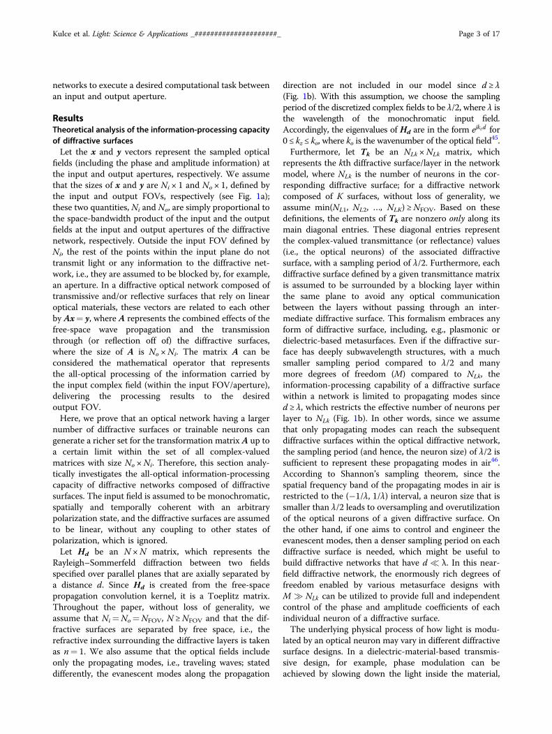
Fig. 1 Schematic of a multisurface diffractive network. aSchematic of a diffractive optical network that connects an input field-of-view (aperture) composed of Ni points to a desired region-of-interest at the output plane/aperture covering No points, throughK-diffractive surfaces with N neurons per surface, sampled at a periodof λ/2n, where λ and n represent the illumination wavelength and therefractive index of the medium between the surfaces, respectively.Without loss of generality, n= 1 was assumed in this paper. b Thecommunication between two successive diffractive surfaces occursthrough propagating waves when the axial separation (d) betweenthese layers is larger than λ. Even if the diffractive surface has deeplysubwavelength structures, as in the case of, e.g., metasurfaces, with amuch smaller sampling period compared to λ/2 and many moredegrees of freedom (M) compared to N, the information-processingcapability of a diffractive surface within a network is limited topropagating modes since d ≥ λ; this limits the effective number ofneurons per layer to N, even for a surface with M >> N. H and H* referto the forward- and backward-wave propagation, respectively

Kulce et al. Light: Science & Applications _#####################_ Page 2 of 17

networks to execute a desired computational task betweenan input and output aperture.

ResultsTheoretical analysis of the information-processing capacityof diffractive surfacesLet the x and y vectors represent the sampled optical

fields (including the phase and amplitude information) atthe input and output apertures, respectively. We assumethat the sizes of x and y are Ni × 1 and No × 1, defined bythe input and output FOVs, respectively (see Fig. 1a);these two quantities, Ni and No, are simply proportional tothe space-bandwidth product of the input and the outputfields at the input and output apertures of the diffractivenetwork, respectively. Outside the input FOV defined byNi, the rest of the points within the input plane do nottransmit light or any information to the diffractive net-work, i.e., they are assumed to be blocked by, for example,an aperture. In a diffractive optical network composed oftransmissive and/or reflective surfaces that rely on linearoptical materials, these vectors are related to each otherby Ax= y, where A represents the combined effects of thefree-space wave propagation and the transmissionthrough (or reflection off of) the diffractive surfaces,where the size of A is No ×Ni. The matrix A can beconsidered the mathematical operator that representsthe all-optical processing of the information carried bythe input complex field (within the input FOV/aperture),delivering the processing results to the desiredoutput FOV.Here, we prove that an optical network having a larger

number of diffractive surfaces or trainable neurons cangenerate a richer set for the transformation matrix A up toa certain limit within the set of all complex-valuedmatrices with size No ×Ni. Therefore, this section analy-tically investigates the all-optical information-processingcapacity of diffractive networks composed of diffractivesurfaces. The input field is assumed to be monochromatic,spatially and temporally coherent with an arbitrarypolarization state, and the diffractive surfaces are assumedto be linear, without any coupling to other states ofpolarization, which is ignored.Let Hd be an N ×N matrix, which represents the

Rayleigh–Sommerfeld diffraction between two fieldsspecified over parallel planes that are axially separated bya distance d. Since Hd is created from the free-spacepropagation convolution kernel, it is a Toeplitz matrix.Throughout the paper, without loss of generality, weassume that Ni=No=NFOV, N ≥NFOV and that the dif-fractive surfaces are separated by free space, i.e., therefractive index surrounding the diffractive layers is takenas n= 1. We also assume that the optical fields includeonly the propagating modes, i.e., traveling waves; stateddifferently, the evanescent modes along the propagation

direction are not included in our model since d ≥ λ(Fig. 1b). With this assumption, we choose the samplingperiod of the discretized complex fields to be λ/2, where λ isthe wavelength of the monochromatic input field.Accordingly, the eigenvalues of Hd are in the form ejkzd for0 ≤ kz ≤ ko, where ko is the wavenumber of the optical field45.Furthermore, let Tk be an NLk ×NLk matrix, which

represents the kth diffractive surface/layer in the networkmodel, where NLk is the number of neurons in the cor-responding diffractive surface; for a diffractive networkcomposed of K surfaces, without loss of generality, weassume min(NL1, NL2, …, NLK) ≥NFOV. Based on thesedefinitions, the elements of Tk are nonzero only along itsmain diagonal entries. These diagonal entries representthe complex-valued transmittance (or reflectance) values(i.e., the optical neurons) of the associated diffractivesurface, with a sampling period of λ/2. Furthermore, eachdiffractive surface defined by a given transmittance matrixis assumed to be surrounded by a blocking layer withinthe same plane to avoid any optical communicationbetween the layers without passing through an inter-mediate diffractive surface. This formalism embraces anyform of diffractive surface, including, e.g., plasmonic ordielectric-based metasurfaces. Even if the diffractive sur-face has deeply subwavelength structures, with a muchsmaller sampling period compared to λ/2 and manymore degrees of freedom (M) compared to NLk, theinformation-processing capability of a diffractive surfacewithin a network is limited to propagating modes sinced ≥ λ, which restricts the effective number of neurons perlayer to NLk (Fig. 1b). In other words, since we assumethat only propagating modes can reach the subsequentdiffractive surfaces within the optical diffractive network,the sampling period (and hence, the neuron size) of λ/2 issufficient to represent these propagating modes in air46.According to Shannon’s sampling theorem, since thespatial frequency band of the propagating modes in air isrestricted to the (−1/λ, 1/λ) interval, a neuron size that issmaller than λ/2 leads to oversampling and overutilizationof the optical neurons of a given diffractive surface. Onthe other hand, if one aims to control and engineer theevanescent modes, then a denser sampling period on eachdiffractive surface is needed, which might be useful tobuild diffractive networks that have d � λ. In this near-field diffractive network, the enormously rich degrees offreedom enabled by various metasurface designs withM � NLk can be utilized to provide full and independentcontrol of the phase and amplitude coefficients of eachindividual neuron of a diffractive surface.The underlying physical process of how light is modu-

lated by an optical neuron may vary in different diffractivesurface designs. In a dielectric-material-based transmis-sive design, for example, phase modulation can beachieved by slowing down the light inside the material,

Kulce et al. Light: Science & Applications _#####################_ Page 3 of 17

where the thickness of an optical neuron determines theamount of phase shift that the light beam undergoes.Alternatively, liquid-crystal-based spatial light modulatorsor flat-optics-based metasurfaces can also be employed aspart of a diffractive network to generate the desired phaseand/or amplitude modulation on the transmitted orreflected light9,47.Starting from “Analysis of a single diffractive surface”, we

investigate the physical properties of A, generated by differ-ent numbers of diffractive surfaces and trainable neurons. Inthis analysis, without loss of generality, each diffractive sur-face is assumed to be transmissive, following the schematicsshown in Fig. 1a, and its extension to reflective surfaces isstraightforward and does not change our conclusions. Finally,multiple (back-and-forth) reflections within a diffractivenetwork composed of different layers are ignored in ouranalysis, as these are much weaker processes compared tothe forward-propagating modes.

Analysis of a single diffractive surfaceThe input–output relationship for a single diffractive

surface that is placed between an input and an outputFOV (Fig. 1a) can be written as

y ¼ H 0d2T1H

0d1x ¼ A1x ð1Þ

where d1 ≥ λ and d2 ≥ λ represent the axial distance betweenthe input plane and the diffractive surface, and the axialdistance between the diffractive surface and the outputplane, respectively. Here we also assume that d1 ≠ d2; theSupplementary Information, Section S5 discusses the specialcase of d1= d2. Since there is only one diffractive surface inthe network, we denote the transmittance matrix as T1, thesize of which is NL1 ×NL1, where L1 represents the diffractivesurface. Here, H 0

d1is an NL1 ×NFOV matrix that is generated

from the NL1 ×NL1 propagation matrix Hd1 by deleting theappropriately chosen NL1−NFOV-many columns. The posi-tions of the deleted columns correspond to the zero-transmission values at the input plane that lie outside theinput FOV or aperture defined by Ni=NFOV (Fig. 1a), i.e.,not included in x. Similarly,H 0

d2is anNFOV ×NL1 matrix that

is generated from the NL1 ×NL1 propagation matrix Hd2 bydeleting the appropriately chosen NL1−NFOV-many rows,which correspond to the locations outside the output FOV oraperture defined by No=NFOV in Fig. 1a; this means that theoutput field is calculated only within the desired outputaperture. As a result, H 0

d1and H 0

d2have a rank of NFOV.

To investigate the information-processing capacity ofA1 based on a single diffractive surface, we vectorizethis matrix in the column order and denote it as vec(A1)= a1

48. Next, we show that the set of possible a1vectors forms a min NL1;N2

FOV

� �-dimensional subset of

the N2FOV-dimensional complex-valued vector space.

The vector, a1, can be written as

vec A1ð Þ ¼ a1 ¼ vec H 0d2T1H 0

d1

� �¼ H 0T

d1�H 0

d2

� �vec T1ð Þ

¼ H 0Td1

�H 0d2

� �t1

ð2Þ

where the superscript T and ⊗ denote the transposeoperation and Kronecker product, respectively48. Here,the size of H 0T

d1�H 0

d2is N2

FOV ´N2L1, and it is a full-rank

matrix with rank N2FOV. In Eq. (2), vec(T1)= t1 has at most

NL1 controllable/adjustable complex-valued entries,which physically represent the neurons of the diffractivesurface, and the rest of its entries are all zero. Thesetransmission coefficients lead to a linear combination ofNL1-many vectors of H 0T

d1�H 0

d2, where d1 ≠ d2 ≠ 0. If

NL1 � N2FOV, these vectors subject to the linear combina-

tion are linearly independent (see the SupplementaryInformation Section S4.1 and Supplementary Fig. S1).Hence, the set of the resulting a1 vectors generated byEq. (2) forms an NL1-dimensional subspace of theN2

FOV-dimensional complex-valued vector space. On theother hand, the vectors in the linear combination start tobecome dependent on each other in the case ofNL1 >N2

FOV and therefore, the dimensionality of the setof possible vector fields is limited to N2

FOV (also seeSupplementary Fig. S1).This analysis demonstrates that the set of complex field

transformation vectors that can be generated by a singlediffractive surface that connects a given input and outputFOV constitutes a min NL1;N2

FOV

� �-dimensional subspace

of the N2FOV-dimensional complex-valued vector space.

These results are based on our earlier assumption thatd1 ≥ λ, d2 ≥ λ, and d1 ≠ d2. For the special case of d1=d2 ≥ λ, the upper limit of the dimensionality of the solu-tion space that can be generated by a single diffractivesurface (K= 1) is reduced from N2

FOV to ðN2FOV þ

NFOVÞ=2 due to the combinatorial symmetries that existin the optical path for d1= d2 (see the SupplementaryInformation, Section S5).

Analysis of an optical network formed by two diffractivesurfacesHere, we consider an optical network with two different

(trainable) diffractive surfaces (K= 2), where theinput–output relation can be written as:

y ¼ H 0d3T2Hd2T1H

0d1x ¼ A2x ð3Þ

Nx ¼ max NL1;NL2ð Þ determines the sizes of the matri-ces in Eq. (3), where NL1 and NL2 represent the number ofneurons in the first and second diffractive surfaces,respectively; d1, d2, and d3 represent the axial distances

Kulce et al. Light: Science & Applications _#####################_ Page 4 of 17

between the diffractive surfaces (see Fig. 1a). Accordingly,the sizes of H 0

d1, Hd2 , and H 0

d3become Nx ×NFOV, Nx ×

Nx, and NFOV ×Nx, respectively. Since we have alreadyassumed that min NL1;NL2ð Þ � NFOV, H 0

d1, and H 0

d3can be

generated from the corresponding Nx ×Nx propagationmatrices by deleting the appropriate columns and rows, asdescribed in “Analysis of a single diffractive surface”.Because Hd2 has a size of Nx ×Nx, there is no need todelete any rows or columns from the associated propa-gation matrix. Although both T1 and T2 have a size ofNx ×Nx, the one corresponding to the diffractive surfacethat contains the smaller number of neurons has somezero values along its main diagonal indices. The numberof these zeros is Nx �min NL1;NL2ð Þ.Similar to the analysis reported in “Analysis of a single

diffractive surface,” the vectorization of A2 reveals

vec A2ð Þ ¼ a2 ¼ vec H 0d3T2Hd2T1H 0

d1

� �¼ H 0T

d1�H 0

d3

� �vec T2Hd2T1ð Þ

¼ H 0Td1

�H 0d3

� �TT

1 � T2� �

vec Hd2ð Þ

¼ H 0Td1

�H 0d3

� �T1 � T2ð Þvec Hd2ð Þ

¼ H 0Td1

�H 0d3

� �T1 � T2ð Þhd2

¼ H 0Td1

�H 0d3

� �Hd2diag T1 � T2ð Þ

¼ H 0Td1

�H 0d3

� �Hd2t12

ð4Þ

where Hd2 is an N2x ´N

2x matrix that has nonzero entries

only along its main diagonal locations. These entriesare generated from vec Hd2ð Þ ¼ hd2 such thatHd2 ½i; i� ¼ hd2 ½i�. Since the diag(·) operator forms a vectorfrom the main diagonal entries of its input matrix, thevector t12 ¼ diag T1 � T2ð Þ is generated such thatt12½i� ¼ T1 � T2ð Þ½i; i�. The equality T1 � T2ð Þhd2 ¼Hd2t12 stems from the fact that the nonzero elements ofT1⊗ T2 are located only along its main diagonal entries.In Eq. (4), H 0T

d1�H 0

d3has rank N2

FOV. Since all thediagonal elements of Hd2 are nonzero, it has rank N

2x . As a

result, HTd1

�Hd3

� �Hd2 is a full-rank matrix with rank

N2FOV. In addition, the nonzero elements of t12 take the

form tij= t1,it2,j, where t1,i and t2,j are the trainable/adjustable complex transmittance values of the ith neuronof the 1st diffractive surface and the jth neuron of the 2nddiffractive surface, respectively, for i∈ {1, 2,…,NL1} andj∈ {1, 2,…, NL2}. Then, the set of possible a2 vectors(Eq. (4)) can be written as

a2 ¼Xi;j

tijhij ð5Þwhere hij is the corresponding column vector ofðH 0T

d1�H 0

d3ÞHd2 .

Equation (5) is in the form of a complex-valued linearcombination of NL1NL2-many complex-valued vectors,hij. Since we assume min(NL1, NL2) ≥NFOV, these vec-tors necessarily form a linearly dependent set of vectorsand this restricts the dimensionality of the vector spaceto N2

FOV. Moreover, due to the coupling of the complex-valued transmittance values of the two diffractive sur-faces (tij= t1,it2,j) in Eq. (5), the dimensionality of theresulting set of a2 vectors can even go below N2

FOV,despite NL1NL2 � N2

FOV. In fact, in “Materials andmethods,” we show that the set of a2 vectors canform an NL1+NL2− 1-dimensional subspace of theN2

FOV-dimensional complex-valued vector space and canbe written as

a2 ¼XNL1þNL2�1

k¼1

ckbk ð6Þ

where bk represents length-N2FOV linearly independent

vectors and ck represents complex-valued coefficients,generated through the coupling of the transmittancevalues of the two independent diffractive surfaces. Therelationship between Eqs. (5) and (6) is also presented as apseudocode in Table 1; see also Supplementary TablesS1–S3 and Supplementary Fig. S2.These analyses reveal that by using a diffractive optical

network composed of two different trainable diffractivesurfaces (with neurons NL1, NL2), it is possible to generatean all-optical solution that spans an NL1+NL2− 1-dimensional subspace of the N2

FOV-dimensional complex-valued vector space. As a special case, if we assumeN ¼ NL1 ¼ NL2 ¼ Ni ¼ No ¼ NFOV, the resulting set ofcomplex-valued linear transformation vectors forms a2N− 1-dimensional subspace of an N2-dimensional vec-tor field. The Supplementary Information (Section S1 andTable S1) also provides a coefficient and basis vectorgeneration algorithm, independently reaching the sameconclusion that this special case forms a 2N− 1-dimen-sional subspace of an N2-dimensional vector field. Theupper limit of the solution space dimensionality that canbe achieved by a two-layered diffractive network is N2

FOV,which is dictated by the input and output FOVs betweenwhich the diffractive network is positioned.In summary, these analyses show that the dimen-

sionality of the all-optical solution space covered bytwo trainable diffractive surfaces (K= 2) positionedbetween a given set of input–output FOV is given bymin N2

FOV;NL1 þNL2 � 1� �

. Different from K= 1 archi-tecture, which revealed a restricted solution space whend1= d2 (see the Supplementary Information, SectionS5), diffractive optical networks with K= 2 do notexhibit a similar restriction related to the axial distancesd1, d2, and d3 (see Supplementary Fig. S2).

Kulce et al. Light: Science & Applications _#####################_ Page 5 of 17

Analysis of an optical network formed by three or morediffractive surfacesNext, we consider an optical network formed by

more than two diffractive surfaces, with neurons of(NL1;NL2; ¼ NLK ) for each layer, where K is the numberof diffractive surfaces and NLk represents the number ofneurons in the kth layer. In the previous section, weshowed that a two-layered network with (NL1, NL2) neu-rons has the same solution space dimensionality as that ofa single-layered, larger diffractive network having NL1+NL2− 1 individual neurons. If we assume that a thirddiffractive surface (NL3) is added to this single-layer net-work with NL1+NL2− 1 neurons, this becomes equiva-lent to a two-layered network with (NL1 þ NL2 � 1;NL3)neurons. Based on “Analysis of an optical network formedby two diffractive surfaces”, the dimensionality of the all-optical solution space covered by this diffractive networkpositioned between a set of input–output FOVs is givenby min N2

FOV;NL1 þ NL2 þ NL3 � 2� �

; also see Supple-mentary Fig. S3 and Supplementary Information SectionS4.3. For the special case of NL1 ¼ NL2 ¼ NL3 ¼Ni ¼ No ¼ N , Supplementary Information Section S2 andTable S2 independently illustrate that the resulting vector

field is indeed a 3N− 2-dimensional subspace of anN2-dimensional vector field.The above arguments can be extended to a network

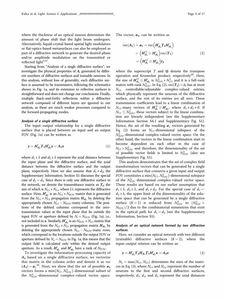
that has K-diffractive surfaces. That is, for a multisurfacediffractive network with a neuron distribution ofðNL1;NL2; ¼ ;NLK Þ, the dimensionality of the solutionspace (see Fig. 2) created by this diffractive network isgiven by

min N2FOV;

XKk¼1

NLk

" #� K � 1ð Þ

!ð7Þ

which forms a subspace of an N2FOV-dimensional vector

space that covers all the complex-valued linear transfor-mations between the input and output FOVs.The upper bound on the dimensionality of the solution

space, i.e., the N2FOV term in Eq. (7), is heuristically

imposed by the number of possible ray interactionsbetween the input and output FOVs. That is, if we con-sider the diffractive optical network as a black box(Fig. 1a), its operation can be intuitively understood ascontrolling the phase and/or amplitude of the light raysthat are collected from the input, to be guided to theoutput, following a lateral grid of λ/2 at the input/outputFOVs, determined by the diffraction limit of light. Thesecond term in Eq. (7), on the other hand, reflects thetotal space-bandwidth product of K-successive diffractivesurfaces, one following another. To intuitively understandthe (K− 1) subtraction term in Eq. (7), one can hypo-thetically consider the simple case of NLk=NFOV= 1for all K-diffractive layers; in this case,½PK

k¼1 NLk � � K � 1ð Þ ¼ 1, which simply indicates that K-successive diffractive surfaces (each with NLk= 1) areequivalent, as physically expected, to a single controllablediffractive surface with NL= 1.Without loss of generality, if we assume N=Nk for all

the diffractive surfaces, then the dimensionality of thelinear transformation solution space created by this dif-fractive network will be KN− (K− 1), provided thatKN � ðK � 1Þ � N2

FOV. The Supplementary Information(Section S3 and Table S3) also provides the same con-clusion. This means that for a fixed design choice of Nneurons per diffractive surface (determined by, e.g., thelimitations of the fabrication methods or other practicalconsiderations), adding new diffractive surfaces to thesame diffractive network linearly increases the dimen-sionality of the solution space that can be all-opticallyprocessed by the diffractive network between the input/output FOVs. As we further increase K such thatKN � ðK � 1Þ � N2

FOV, the diffractive network reaches itslinear transformation capacity, and adding more layers ormore neurons to the network does not further contributeto its processing power for the desired input–outputFOVs (see Fig. 2). However, these deeper diffractive

Table 1 Coefficient (ck) and basis vector (bk) generationalgorithm pseudocode for an optical network that has twodiffractive surfaces

1 Randomly choose t1,i from the set C1,1 and t2,j from the set C2,1, and

assign desired values to the chosen t1,i and t2,j

2 c1b1 ¼ t1;it2;jhij

3 k= 2

4 Randomly choose T1 or T2 if C1;k ≠ ; and C2;k ≠ ;Choose T1 if C1;k ≠ ; and C2;k ¼ ;Choose T2 if C1;k ¼ ; and C2;k ≠ ;

5 If T1 is chosen in Step 4:

6 Randomly choose t1,i from the set C1,k, and assign a desired value to

the chosen t1,i

7 ckbk ¼ t1;iP

t2;j=2C2;kt2;jhij

� �8 else:

9 Randomly choose t2,j from the set C2,k, and assign a desired value to

the chosen t2,j

10 ckbk ¼ t2;jP

t1;i=2C1;kt1;ihij

� �11 k= k+ 1

12 If C1;k ≠ ; or C2;k ≠ ;:13 Return to Step 4

14 else:

15 Exit

See the theoretical analysis and Eq. (6) of the main text. See also SupplementaryTables S1–S3

Kulce et al. Light: Science & Applications _#####################_ Page 6 of 17

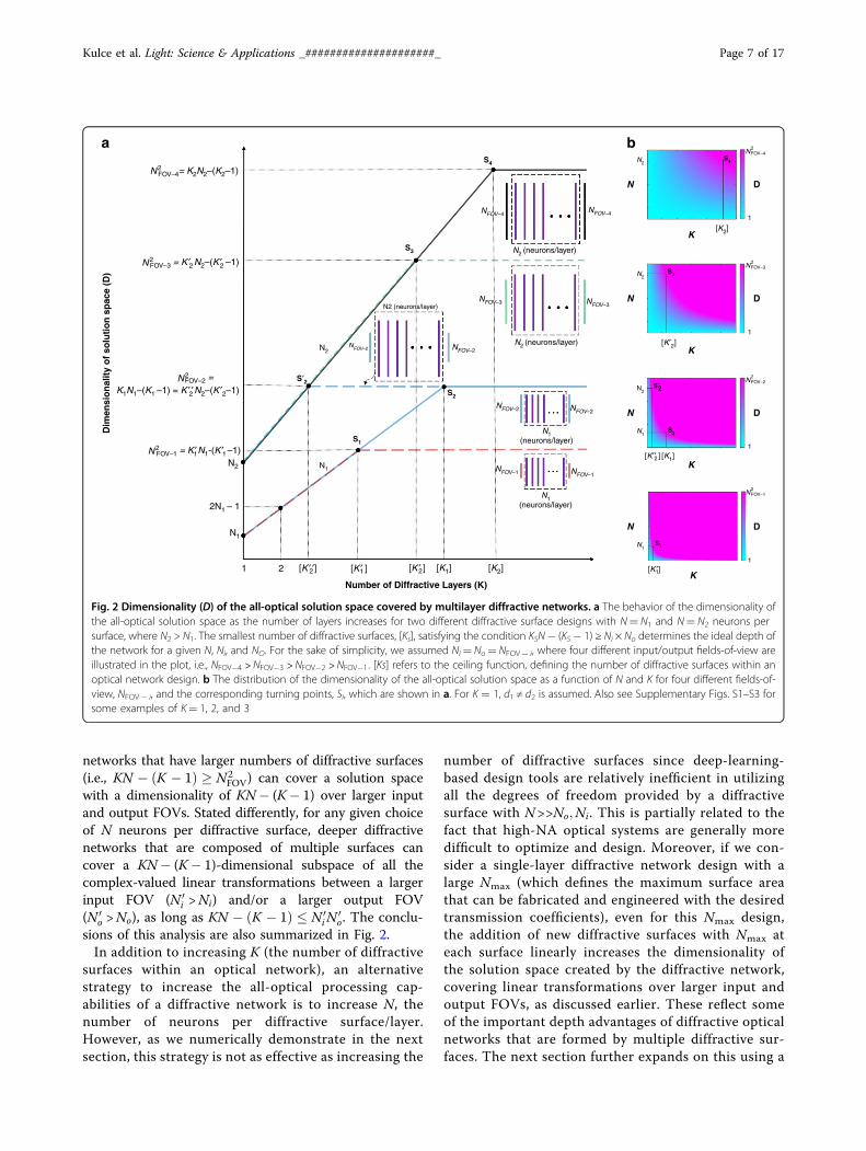
networks that have larger numbers of diffractive surfaces(i.e., KN � ðK � 1Þ � N2

FOV) can cover a solution spacewith a dimensionality of KN− (K− 1) over larger inputand output FOVs. Stated differently, for any given choiceof N neurons per diffractive surface, deeper diffractivenetworks that are composed of multiple surfaces cancover a KN− (K− 1)-dimensional subspace of all thecomplex-valued linear transformations between a largerinput FOV (N 0

i >Ni) and/or a larger output FOV(N 0

o >No), as long as KN � ðK � 1Þ � N 0iN

0o. The conclu-

sions of this analysis are also summarized in Fig. 2.In addition to increasing K (the number of diffractive

surfaces within an optical network), an alternativestrategy to increase the all-optical processing cap-abilities of a diffractive network is to increase N, thenumber of neurons per diffractive surface/layer.However, as we numerically demonstrate in the nextsection, this strategy is not as effective as increasing the

number of diffractive surfaces since deep-learning-based design tools are relatively inefficient in utilizingall the degrees of freedom provided by a diffractivesurface with N>>No;Ni. This is partially related to thefact that high-NA optical systems are generally moredifficult to optimize and design. Moreover, if we con-sider a single-layer diffractive network design with alarge Nmax (which defines the maximum surface areathat can be fabricated and engineered with the desiredtransmission coefficients), even for this Nmax design,the addition of new diffractive surfaces with Nmax ateach surface linearly increases the dimensionality ofthe solution space created by the diffractive network,covering linear transformations over larger input andoutput FOVs, as discussed earlier. These reflect someof the important depth advantages of diffractive opticalnetworks that are formed by multiple diffractive sur-faces. The next section further expands on this using a

N2

[K2]1

DN

K

N2

[K′2]1

DN

K

S4S4

S3

S2

S1

S2

S3

S2

S′2

S1

N1

N2

N2

N1

N1(neurons/layer)

N1(neurons/layer)

N2 (neurons/layer)

N2 (neurons/layer)

[K1][K′′ ]1

DN

K2

[K ′ ′]2 [K ′ ]1 [K ′ ]2 [K1] [K2]

N2

N1

[K ′]

FOV–1

N2FOV–2

N2FOV–3

N2FOV–4

1

DN

K1

NFOV–4NFOV–4

NFOV–3

NFOV–2NFOV–2

NFOV–2

NFOV–1

NFOV–3

NFOV–2

NFOV–1

N2 (neurons/layer)

1 2

Number of Diffractive Layers (K)

N1

2N1 – 1

N2

N2

N2

FOV–1 = K ′N1-(K ′ –1)1 1

K1N1–(K1 –1) = K ′ ′N2–(K ′ –1)2 2

FOV–3 = K ′ N2–(K ′ –1)2 2

FOV–2 =

N2

FOV–4= K2N2–(K2–1)N2

Dim

ensi

on

alit

y o

f so

luti

on

sp

ace

(D)

a b

Fig. 2 Dimensionality (D) of the all-optical solution space covered by multilayer diffractive networks. a The behavior of the dimensionality ofthe all-optical solution space as the number of layers increases for two different diffractive surface designs with N= N1 and N= N2 neurons persurface, where N2 > N1. The smallest number of diffractive surfaces, [Ks], satisfying the condition KSN− (KS− 1) ≥ Ni × No determines the ideal depth ofthe network for a given N, Ni, and NO. For the sake of simplicity, we assumed Ni= No= NFOV− i, where four different input/output fields-of-view areillustrated in the plot, i.e., NFOV�4 >NFOV�3 >NFOV�2 >NFOV�1. [Ks] refers to the ceiling function, defining the number of diffractive surfaces within anoptical network design. b The distribution of the dimensionality of the all-optical solution space as a function of N and K for four different fields-of-view, NFOV− i, and the corresponding turning points, Si, which are shown in a. For K = 1, d1 ≠ d2 is assumed. Also see Supplementary Figs. S1–S3 forsome examples of K= 1, 2, and 3

Kulce et al. Light: Science & Applications _#####################_ Page 7 of 17

numerical analysis of diffractive optical networks thatare designed for image classification.

Numerical analysis of diffractive networksThe previous section showed that the dimensionality of

the all-optical solution space covered by K-diffractivesurfaces, forming an optical network positioned betweenan input and output FOV, is determined byminðN2

FOV; ½PK

k¼1 NLk � � K � 1ð ÞÞ. However, this mathe-matical analysis does not shed light on the selection oroptimization of the complex transmittance (or reflec-tance) values of each neuron of a diffractive network thatis assigned for a given computational task. Here, wenumerically investigate the function approximation powerof multiple diffractive surfaces in the (N, K) space usingimage classification as a computational goal for the designof each diffractive network. Since NFOV and N are largenumbers in practice, an iterative optimization procedurebased on error back-propagation and deep learning with adesired loss function was used to design diffractive net-works and compare their performances as a functionof (N, K).For the first image classification task that was used as a

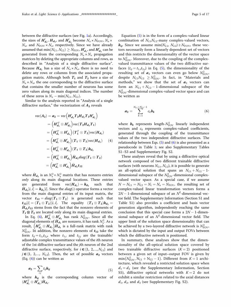
test bed, we formed nine different image data classes,where the input FOV (aperture) was randomly dividedinto nine different groups of pixels, each group definingone image class (Fig. 3a). Images of a given data class canhave pixels only within the corresponding group, emittinglight at arbitrary intensities toward the diffractive net-work. The computational task of each diffractive networkis to blindly classify the input images from one of thesenine different classes using only nine large-area detectorsat the output FOV (Fig. 3b), where the classificationdecision is made based on the maximum of the opticalsignal collected by these nine detectors, each assigned toone particular image class. For deep-learning-basedtraining of each diffractive network for this image classi-fication task, we employed a cross-entropy loss function(see “Materials and methods”).Before we report the results of our analysis using a more

standard image classification dataset such as CIFAR-1049,we initially selected this image classification problemdefined in Fig. 3 as it provides a well-defined lineartransformation between the input and output FOVs. Italso has various implications for designing new imagingsystems with unique functionalities that cannot be cov-ered by standard lens design principles.Based on the diffractive network configuration and the

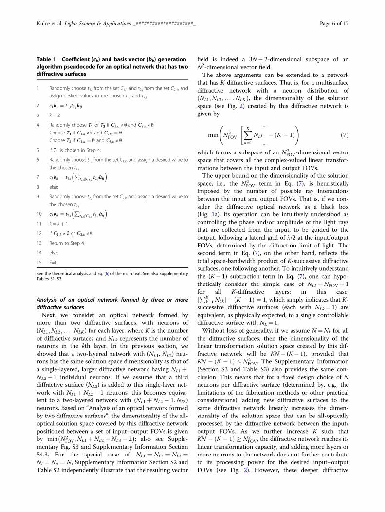
image classification problem depicted in Fig. 3, we com-pared the training and blind-testing accuracies providedby different diffractive networks composed of 1, 2, and 3diffractive surfaces (each surface having N= 40K= 200 ×200 neurons) under different training and testing condi-tions (see Figs. 4 and 5). Our analysis also included the

performance of a wider single-layer diffractive networkwith N= 122.5K > 3 × 40K neurons. For the training ofthese diffractive systems, we created two different trainingimage sets (Tr1 and Tr2) to test the learning capabilitiesof different network architectures. In the first case, thetraining samples were selected such that approximately1% of the point sources defining each image data classwere simultaneously on and emitting light at variouspower levels. For this training set, 200K images werecreated, forming Tr1. In the second case, the trainingimage dataset was constructed to include only a singlepoint source (per image) located at different coordinatesrepresenting different data classes inside the input FOV,providing us with a total of 6.4K training images (whichformed Tr2). For the quantification of the blind-testingaccuracies of the trained diffractive models, three differenttest image datasets (never used during the training) werecreated, with each dataset containing 100K images. Thesethree distinct test datasets (named Te1, Te50, and Te90)contain image samples that take contributions from 1%(Te1), 50% (Te50), and 90% (Te90) of the points definingeach image data class (see Fig. 3).Figure 4 illustrates the blind classification accuracies

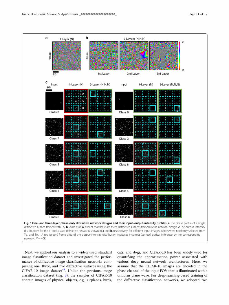
achieved by the different diffractive network models thatwe trained. We see that as the number of diffractivesurfaces in the network increases, the testing accuraciesachieved by the final diffractive design improve sig-nificantly, meaning that the linear transformation spacecovered by the diffractive network expands with theaddition of new trainable diffractive surfaces, in line withour former theoretical analysis. For instance, while a dif-fractive image classification network with a single phase-only (complex) modulation surface can achieve 24.48%(27.00%) for the test image set Te1, the three-layer ver-sions of the same architectures attain 85.2% (100.00%)blind-testing accuracies, respectively (see Fig. 4a, b).Figure 5 shows the phase-only diffractive layers com-prising the 1- and 3-layer diffractive optical networks thatare compared in Fig. 4a; Fig. 5 also reports someexemplary test images selected from Te1 and Te50, alongwith the corresponding intensity distributions at theoutput planes of the diffractive networks. The comparisonbetween two- and three-layer diffractive systems alsoindicates a similar conclusion for the test image set, Te1.However, as we increase the number of point sourcescontributing to the test images, e.g., for the case of Te90,the blind-testing classification accuracies of both the two-and three-layer networks saturate at nearly 100%, indi-cating that the solution space of the two-layer networkalready covers the optical transformation required toaddress this relatively easier image classification problemset by Te90.A direct comparison between the classification

accuracies reported in Fig. 4a–d further reveals that the

Kulce et al. Light: Science & Applications _#####################_ Page 8 of 17

InputData class 0Data class 1Data class 2Data class 3Data class 4Data class 5Data class 6Data class 7Data class 8

Output

0 1 2

3 4 5

6 7 8

Inpu

t

Output

Data class 2Data class 1Data class 0

Data class 4Data class 5

Dat

a cl

ass

3

Data class 7

Data class 6

Data class 8

20�20�

a

d

b c

Fig. 3 Spatially encoded image classification dataset. a Nine image data classes are shown (presented in different colors), defined inside the inputfield-of-view (80λ × 80λ). Each λ × λ area inside the field-of-view is randomly assigned to one image data class. An image belongs to a given data classif and only if all of its nonzero entries belong to the pixels that are assigned to that particular data class. b The layout of the nine class detectorspositioned at the output plane. Each detector has an active area of 25λ × 25λ, and for a given input image, the decision on class assignment is madebased on the maximum optical signal among these nine detectors. c Side view of the schematic of the diffractive network layers, as well as the inputand output fields-of-view. d Example images for nine different data classes. Three samples for each image data class are illustrated here, randomlydrawn from the three test datasets (Te1, Te50, and Te90) that were used to quantify the blind inference accuracies of our diffractive network models(see Fig. 4)

Kulce et al. Light: Science & Applications _#####################_ Page 9 of 17

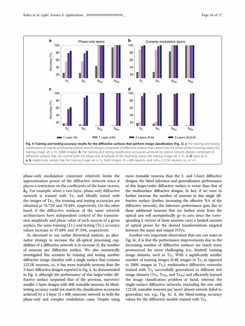
phase-only modulation constraint relatively limits theapproximation power of the diffractive network since itplaces a restriction on the coefficients of the basis vectors,hij. For example, when a two-layer, phase-only diffractivenetwork is trained with Tr1 and blindly tested withthe images of Te1, the training and testing accuracies areobtained as 78.72% and 78.44%, respectively. On the otherhand, if the diffractive surfaces of the same networkarchitectures have independent control of the transmis-sion amplitude and phase value of each neuron of a givensurface, the same training (Tr1) and testing (Te1) accuracyvalues increase to 97.68% and 97.39%, respectively.As discussed in our earlier theoretical analysis, an alter-

native strategy to increase the all-optical processing cap-abilities of a diffractive network is to increase N, the numberof neurons per diffractive surface. We also numericallyinvestigated this scenario by training and testing anotherdiffractive image classifier with a single surface that contains122.5K neurons, i.e., it has more trainable neurons than the3-layer diffractive designs reported in Fig. 4. As demonstratedin Fig. 4, although the performance of this larger/wider dif-fractive surface surpassed that of the previous, narrower/smaller 1-layer designs with 40K trainable neurons, its blind-testing accuracy could not match the classification accuraciesachieved by a 2-layer (2 × 40K neurons) network in both thephase-only and complex modulation cases. Despite using

more trainable neurons than the 2- and 3-layer diffractivedesigns, the blind inference and generalization performanceof this larger/wider diffractive surface is worse than that ofthe multisurface diffractive designs. In fact, if we were tofurther increase the number of neurons in this single dif-fractive surface (further increasing the effective NA of thediffractive network), the inference performance gain due tothese additional neurons that are farther away from theoptical axis will asymptotically go to zero since the corre-sponding k vectors of these neurons carry a limited amountof optical power for the desired transformations targetedbetween the input and output FOVs.Another very important observation that one can make in

Fig. 4c, d is that the performance improvements due to theincreasing number of diffractive surfaces are much morepronounced for more challenging (i.e., limited) trainingimage datasets, such as Tr2. With a significantly smallernumber of training images (6.4K images in Tr2 as opposedto 200K images in Tr1), multisurface diffractive networkstrained with Tr2 successfully generalized to different testimage datasets (Te1, Te50, and Te90) and efficiently learnedthe image classification problem at hand, whereas thesingle-surface diffractive networks (including the one with122.5K trainable neurons per layer) almost entirely failed togeneralize; see, e.g., Fig. 4c, d, the blind-testing accuracyvalues for the diffractive models trained with Tr2.

Phase-only layers Complex modulation layers100

80

60

40

20

100

80

60

40

20

Acc

urac

y (%

)

100

80

60

40

20

100

80

60

40

20

Acc

urac

y (%

)

Tr1 Te1 Te50 Te90 Tr1 Te1 Te50 Te90

Tr2 Te1 Te50 Te90 Tr2 Te1 Te50 Te90

1 Layer (N) 1 Layer (mN) 2 Layers (N,N) 3 Layers (N,N,N)

a b

c d

Fig. 4 Training and testing accuracy results for the diffractive surfaces that perform image classification (Fig. 3). a The training and testingclassification accuracies achieved by optical network designs composed of diffractive surfaces that control only the phase of the incoming waves; thetraining image set is Tr1 (200K images). b The training and testing classification accuracies achieved by optical network designs composed ofdiffractive surfaces that can control both the phase and amplitude of the incoming waves; the training image set is Tr1. c, d Same as ina, b, respectively, except that the training image set is Tr2 (6.4K images). N= 40K neurons, and mN= 122.5K neurons, i.e., m > 3

Kulce et al. Light: Science & Applications _#####################_ Page 10 of 17

Next, we applied our analysis to a widely used, standardimage classification dataset and investigated the perfor-mance of diffractive image classification networks com-prising one, three, and five diffractive surfaces using theCIFAR-10 image dataset49. Unlike the previous imageclassification dataset (Fig. 3), the samples of CIFAR-10contain images of physical objects, e.g., airplanes, birds,

cats, and dogs, and CIFAR-10 has been widely used forquantifying the approximation power associated withvarious deep neural network architectures. Here, weassume that the CIFAR-10 images are encoded in thephase channel of the input FOV that is illuminated with auniform plane wave. For deep-learning-based training ofthe diffractive classification networks, we adopted two

1 Layer (N) 3 Layers (N,N,N)

Pha

se

Pha

se

20�

20�

1st Layer 2nd Layer 3rd Layer

�

–�

Input 1-Layer (N) 3-Layer (N,N,N) Input 1-Layer (N) 3-Layer (N,N,N)

Class 0

Class 7

Class 3

Class 1

Class 5 Class 6

Class 4

Class 8

Class 2

Class 8

0 1 2

3 4 5

6 7 8

a

c

b

Fig. 5 One- and three-layer phase-only diffractive network designs and their input–output-intensity profiles. a The phase profile of a singlediffractive surface trained with Tr1. b Same as in a, except that there are three diffractive surfaces trained in the network design. c The output-intensitydistributions for the 1- and 3-layer diffractive networks shown in a and b, respectively, for different input images, which were randomly selected fromTe1 and Te50. A red (green) frame around the output-intensity distribution indicates incorrect (correct) optical inference by the correspondingnetwork. N= 40K.

Kulce et al. Light: Science & Applications _#####################_ Page 11 of 17

different loss functions. The first loss function is based onthe mean-squared error (MSE), which essentially for-mulates the design of the all-optical object classificationsystem as an image transformation/projection problem,and the second one is based on the cross-entropy loss,which is commonly used to solve the multiclass separa-tion problems in the deep-learning literature (refer to“Materials and methods” for details).The results of our analysis are summarized in Fig. 6a, b,

which report the average blind inference accuracies alongwith the corresponding standard deviations observed overthe testing of three different diffractive network modelstrained independently to classify the CIFAR-10 test ima-ges using phase-only and complex-valued diffractive sur-faces, respectively. The 1-, 3-, and 5-layer phase-only(complex-valued) diffractive network architectures canattain blind classification accuracies of 40.55∓ 0.10%(41.52∓ 0.09%), 44.47∓ 0.14% (45.88∓ 0.28%), and45.53∓ 0.30% (46.84∓ 0.46%), respectively, when they aretrained based on the cross-entropy loss detailed in“Materials and methods”. On the other hand, with the use

of the MSE loss, these classification accuracies arereduced to 16.25 ∓ 0.48% (14.92∓ 0.26%), 29.08∓ 0.14%(33.52∓ 0.40%), and 33.67 ∓ 0.57% (34.69∓ 0.11%),respectively. In agreement with the conclusions of ourprevious results and the presented theoretical analysis, theblind-testing accuracies achieved by the all-optical dif-fractive classifiers improve with increasing the number ofdiffractive layers, K, independent of the loss function usedand the modulation constraints imposed on the trainedsurfaces (see Fig. 6).Different from electronic neural networks, however,

diffractive networks are physical machine-learning plat-forms with their own optical hardware; hence, practicaldesign merits such as the signal-to-noise ratio (SNR) andthe contrast-to-noise ratio (CNR) should also be con-sidered, as these features can be critical for the success ofthese networks in various applications. Therefore, inaddition to the blind-testing accuracies, the performanceevaluation and comparison of these all-optical diffractiveclassification systems involve two additional metrics thatare analogous to the SNR and CNR. The first is the

Phase-only layers Complex modulation layers

Cross-entropy

MSE

50

40

30

20

10

30

20

102

101

100

46

44

42

40

15

14

15

11

Test

ing

accu

racy

(%

)

Test

ing

accu

racy

(%

)Testing accuracy (%)

Cla

ssifi

catio

n ef

ficie

ncy

(%)

Opt

ical

sig

nal c

ontr

ast (

%)

15

41

43

45

47

14

15

11

Cla

ssifi

catio

n ef

ficie

ncy

(%)

Opt

ical

sig

nal c

ontr

ast (

%)

Classification efficiency (%

)O

ptical signal contrast (%)

50

40

30

20

10

30

20

102

101

100

Testing accuracy (%)

Classification efficiency (%

)O

ptical signal contrast (%)

1 3 5

Numbar of diffractive layers

1 3 5

Numbar of diffractive layers

a b

Fig. 6 Comparison of the 1-, 3-, and 5-layer diffractive networks trained for CIFAR-10 image classification using the MSE and cross-entropyloss functions. a Results for diffractive surfaces that modulate only the phase information of the incoming wave. b Results for diffractive surfaces thatmodulate both the phase and amplitude information of the incoming wave. The increase in the dimensionality of the all-optical solution space withadditional diffractive surfaces of a network brings significant advantages in terms of generalization, blind-testing accuracy, classification efficiency,and optical signal contrast. The classification efficiency denotes the ratio of the optical power detected by the correct class detector with respect tothe total detected optical power by all the class detectors at the output plane. Optical signal contrast refers to the normalized difference between theoptical signals measured by the ground-truth (correct) detector and its strongest competitor detector at the output plane

Kulce et al. Light: Science & Applications _#####################_ Page 12 of 17

classification efficiency, which we define as the ratio of theoptical signal collected by the target, ground-truth classdetector, Igt, with respect to the total power collected byall class detectors located at the output plane. The secondperformance metric refers to the normalized differencebetween the optical signals measured by the ground-truth/correct detector, Igt, and its strongest competitor,Isc, i.e., ðIgt � IscÞ=Igt ; this optical signal contrast metric is,in general, important since the relative level of detectionnoise with respect to this difference is critical for trans-lating the accuracies achieved by the numerical forwardmodels to the performance of the physically fabricateddiffractive networks. Figure 6 reveals that the improve-ments observed in the blind-testing accuracies as afunction of the number of diffractive surfaces also apply tothese two important diffractive network performancemetrics, resulting from the increased dimensionality ofthe all-optical solution space of the diffractive networkwith increasing K. For instance, the diffractive networkmodels presented in Fig. 6b, trained with the cross-entropy (or MSE) loss function, provide classificationefficiencies of 13.72∓ 0.03% (13.98∓ 0.12%), 15.10∓0.08% (31.74∓ 0.41%), and 15.46∓ 0.08% (34.43∓ 0.28%)using complex-valued 1, 3, and 5 layers, respectively.Furthermore, the optical signal contrast attained by thesame diffractive network designs can be calculated as10.83∓ 0.17% (9.25∓ 0.13%), 13.92∓ 0.28% (35.23∓1.02%), and 14.88∓ 0.28% (38.67∓ 0.13%), respectively.Similar improvements are also observed for the phase-only diffractive optical network models that are reportedin Fig. 6a. These results indicate that the increaseddimensionality of the solution space with increasing Kimproves the inference capacity as well as the robustnessof the diffractive network models by enhancing theiroptical efficiency and signal contrast.Apart from the results and analyses reported in this sec-

tion, the depth advantage of diffractive networks has beenempirically shown in the literature for some other applica-tions and datasets, such as, e.g., image classification38,40 andoptical spectral filter design42.

DiscussionIn a diffractive optical design problem, it is not

guaranteed that the diffractive surface profiles willconverge to the optimum solution for a given (N, K)configuration. Furthermore, for most applications ofinterest, such as image classification, the optimumtransformation matrix that the diffractive surfaces needto approximate is unknown; for example, what definesall the images of cats versus dogs (such as in theCIFAR-10 image dataset) is not known analytically tocreate a target transformation. Nonetheless, it can beargued that as the dimensionality of the all-opticalsolution space, and thus the approximation power of

the diffractive surfaces, increases, the probability ofconverging to a solution satisfying the desired designcriteria also increases. In other words, even if theoptimization of the diffractive surfaces becomes trap-ped in a local minimum, which is practically always thecase, there is a greater chance that this state will becloser to the globally optimal solution(s) for deeperdiffractive networks with multiple trainable surfaces.Although not considered in our analysis thus far, an

interesting future direction to investigate is the case wherethe axial distance between two successive diffractive sur-faces is made much smaller than the wavelength of light,i.e., d≪ λ. In this case, all the evanescent waves and thesurface modes of each diffractive layer will need to becarefully taken into account to analyze the all-opticalprocessing capabilities of the resulting diffractive network.This would significantly increase the space-bandwidthproduct of the optical processor as the effective neuronsize per diffractive surface/layer can be deeply sub-wavelength if the near-field is taken into account. Fur-thermore, due to the presence of near-field couplingbetween diffractive surfaces/layers, the effective transmis-sion or reflection coefficient of each neuron of a surfacewill no longer be an independent parameter, as it willdepend on the configuration/design of the other surfaces. Ifall of these near-field-related coupling effects are carefullytaken into consideration during the design of a diffractiveoptical network with d≪ λ, it can significantly enrich thesolution space of multilayer coherent optical processors,assuming that the surface fabrication resolution and theSNR as well as the dynamic range at the detector plane areall sufficient. Despite the theoretical richness of near-field-based diffractive optical networks, the design and imple-mentation of these systems bring substantial challenges interms of their 3D fabrication and alignment, as well as theaccuracy of the computational modeling of the associatedphysics within the diffractive network, including multiplereflections and boundary conditions. While various elec-tromagnetic wave solvers can handle the numerical analysisof near-field diffractive systems, practical aspects of a fab-ricated near-field diffractive neural network will presentvarious sources of imperfections and errors that mightforce the physical forward model to significantly deviatefrom the numerical simulations.In summary, we presented a theoretical and numerical

analysis of the information-processing capacity and functionapproximation power of diffractive surfaces that can com-pute a given task using temporally and spatially coherentlight. In our analysis, we assumed that the polarization stateof the propagating light is preserved by the optical modula-tion on the diffractive surfaces, and that the axial distancebetween successive layers is kept large enough to ensure thatthe near-field coupling and related effects can be ignored inthe optical forward model. Based on these assumptions, our

Kulce et al. Light: Science & Applications _#####################_ Page 13 of 17

analysis shows that the dimensionality of the all-opticalsolution space provided by multilayer diffractive networksexpands linearly as a function of the number of trainablesurfaces, K, until it reaches the limit defined by the targetinput and output FOVs, i.e., minðN2

FOV; ½PK

k¼1 NLk ��K � 1ð ÞÞ, as depicted in Eq. (7) and Fig. 2. To numericallyvalidate these conclusions, we adopted a deep-learning-basedtraining strategy to design diffractive image classificationsystems for two distinct datasets (Figs. 3–6) and investigatedtheir performance in terms of blind inference accuracy,learning and generalization performance, classification effi-ciency, and optical signal contrast, confirming the depthadvantages provided by multiple diffractive surfaces com-pared to a single diffractive layer.These results and conclusions, along with the underlying

analyses, broadly cover various types of diffractive surfaces,including, e.g., metamaterials/metasurfaces, nanoantennaarrays, plasmonics, and flat-optics-based designer surfaces.We believe that the deeply subwavelength design features of,e.g., diffractive metasurfaces, can open up new avenues in thedesign of coherent optical processers by enabling indepen-dent control over the amplitude and phase modulation ofneurons of a diffractive layer, also providing unique oppor-tunities to engineer the material dispersion properties asneeded for a given computational task.

Materials and methodsCoefficient and basis vector generation for an opticalnetwork formed by two diffractive surfacesHere, we present the details of the coefficient and basis

vector generation algorithm for a network having two dif-fractive surfaces with the neurons (NL1,NL2) to show that it iscapable of forming a vectorized transformation matrix in anNL1+NL2− 1-dimensional subspace of an N2

FOV-dimen-sional complex-valued vector space. The algorithm dependson the consumption of the transmittance values from thefirst or the second diffractive layer, i.e., T1 or T2, at each stepafter its initialization. A random neuron is first chosen fromT1 or T2, and then a new basis vector is formed. The chosenneuron becomes the coefficient of this new basis vector,which is generated by using the previously chosen trans-mittance values and appropriate vectors from hij (Eq. (5)).The algorithm continues until all the transmittance valuesare assigned to an arbitrary complex-valued coefficient anduses all the vectors of hij in forming the basis vectors.In Table 1, a pseudocode of the algorithm is also presented.

In this table, C1,k and C2,k represent the sets of transmittancevalues that include t1,i and t2,j, which were not chosen before(at time step k), from the first and second diffractive surfaces,respectively. In addition, ck= t1,i in Step 7 and ck= t2,j in Step10 are the complex-valued coefficients that can be inde-pendently determined. Similarly, bk ¼Pt2;j=2C2;k

t2;jhij andbk ¼Pt1;i=2C1;k

t1;ihij are the basis vectors generated at eachstep, where t1;i=2C1;k and t2;j=2C2;k represent the sets of

coefficients that are chosen before. The basis vectors in Steps7 and 10 are formed through the linear combinations of thecorresponding hij vectors.By examining the algorithm in Table 1, it is straightfor-

ward to show that the total number of generated basisvectors is NL1+NL2− 1. That is, at each time step k, onlyone coefficient either from the first or the second layer ischosen, and only one basis vector is created. Since there areNL1+NL2-many transmittance values where two of themare chosen together in Step 1, the total number of time steps(coefficient and basis vectors) becomes NL1+NL2− 1. Onthe other hand, showing that all the NL1NL2-many hij vectorsare used in the algorithm requires further analysis. Withoutloss of generality, let T1 be chosen n1 times starting from thetime step k= 2, and then T2 is chosen n2 times. Similarly, T1

and T2 are chosen n3 and n4 times in the following cycles,respectively. This pattern continues until allNL1+NL2-manytransmittance values are consumed. Here, we show thepartition of the selection of the transmittance values from T1

and T2 for each time step k into s-many chunks, i.e.,

k ¼ 2; 3; ¼|fflfflfflffl{zfflfflfflffl}n1

; ¼|{z}n2

; ¼|{z}n3

; ¼|{z}n4

; ¼ ; ¼NL1 þ NL2 � 2;NL1 þ NL2 � 1|fflfflfflfflfflfflfflfflfflfflfflfflfflfflfflfflfflfflfflfflfflfflfflfflfflfflfflfflffl{zfflfflfflfflfflfflfflfflfflfflfflfflfflfflfflfflfflfflfflfflfflfflfflfflfflfflfflfflffl}ns

8<:

9=;ð8Þ

To show that NL1NL2-many hij vectors are used in thealgorithm regardless of the values of s and ni, we first define

pi ¼ ni þ pi�2 for even values of i � 2

qi ¼ ni þ qi�2 for odd values of i � 1

where p0= 0 and q−1= 1. Based on this, the total numberof consumed basis vectors inside each summation inTable 1 (Steps 7 and 10) can be written as

nh ¼ 1þ Pq1k¼2

1þ Pp2þq1

k¼q1þ1q1 þ

Pq3þp2

k¼p2þq1þ1ðp2 þ 1Þ þ Pp4þq3

k¼q3þp2þ1q3

þ Pq5þp4

k¼p4þq3þ1ðp4 þ 1Þ þ Pp6þq5

k¼q5þp4þ1q5 þ

Pq7þp6

k¼p6þq5þ1ðp6 þ 1Þ

þ¼ þ PNL1þps�2

k¼ps�2þqs�3þ1ðps�2 þ 1Þ þ PNL1þNL2�1

k¼NL1þps�2þ1NL1

ð9Þwhere each summation gives the number of consumed hijvectors in the corresponding chunk. Please note thatbased on the partition given by Eq. (8), qs−1 and psbecome equal to NL1 and NL2− 1, respectively. One canshow, by carrying out this summation, that all the termsexcept NL1NL2 cancel each other out, and therefore, nh=NL1NL2, demonstrating that all the NL1NL2-many hijvectors are used in the algorithm. Here, we assumed thatthe transmittance values from the first diffractive layer areconsumed first. However, even if it were assumed that the

Kulce et al. Light: Science & Applications _#####################_ Page 14 of 17

transmittance values from the second diffractive layer areconsumed first, the result does not change (also seeSupplementary Information Section S4.2 and Fig. S2).The Supplementary Information and Table S1 also report

an independent analysis of the special case for NL1 ¼ NL2 ¼Ni ¼ No ¼ N and Table S3 reports the special case of NL2 ¼Ni ¼ No ¼ N and NL1 ¼ ðK � 1ÞN � ðK � 2Þ, all of whichconfirm the conclusions reported here. The SupplementaryInformation also includes an analysis of the coefficient andbasis vector generation algorithm for a network formed bythree diffractive surfaces (K= 3) when NL1 ¼ NL2 ¼ NL3 ¼Ni ¼ No ¼ N (see Table S2); also see SupplementaryInformation Section S4.3 and Supplementary Fig. S3 foradditional numerical analysis of K= 3 case, further con-firming the same conclusions.

Optical forward modelIn a coherent optical processor composed of diffractive

surfaces, the optical transformation between a given pairof input/output FOVs is established through the mod-ulation of light by a series of diffractive surfaces, which wemodeled as two-dimensional, thin, multiplicative ele-ments. According to our formulation, the complex-valuedtransmittance of a diffractive surface, k, is defined as

t x; y; zkð Þ ¼ a x; yð Þ exp j2πϕ x; yð Þð Þ ð10Þ

where a(x, y) and ϕ(x, y) denote the trainable amplitudeand the phase modulation functions of diffractive layer k.The values of a(x, y), in general, lie in the interval (0, 1),i.e., there is no optical gain over these surfaces, and thedynamic range of the phase modulation is between (0,2π). In the case of phase-only modulation restriction,however, a(x, y) is kept as 1 (nontrainable) for all theneurons. The parameter zk defines the axial location ofthe diffractive layer k between the input FOV at z= 0and the output plane. Based on these assumptions, theRayleigh–Sommerfeld formulation expresses the lightdiffraction by modeling each diffractive unit on layer k at(xq, yq, zk) as the source of a secondary wave

wkq x; y; zð Þ ¼ z � zk

r21

2πrþ 1jλ

� �exp

j2πrλ

� �ð11Þ

where r ¼ffiffiffiffiffiffiffiffiffiffiffiffiffiffiffiffiffiffiffiffiffiffiffiffiffiffiffiffiffiffiffiffiffiffiffiffiffiffiffiffiffiffiffiffiffiffiffiffiffiffiffiffiffiffiffiffiffiffiffiffiffiffiffix� xq� �2þ y� xq

� �2þ z � zkð Þ2q

. CombiningEqs. (10) and (11), we can write the light field exiting theqth diffractive unit of layer k+ 1 as

ukþ1q x; y; zð Þ ¼ t xq; yq; zkþ1

� �wkþ1q x; y; zð ÞX

p2 Sk

ukp xq; yq; zkþ1� � ð12Þ

where Sk denotes the set of diffractive units of layer k.From Eq. (12), the complex wave field at the output plane

can be written as

uKþ1 x; y; zð Þ ¼ Pq2 SK

t xq; yq; zK� �

wKq x; y; zð Þ P

p2 SK�1

uK�1p xq; yq; zK� �" #

ð13Þwhere the optical field immediately after the object isassumed to be u0(x, y, z). In Eq. (13), SK and SK− 1 denotethe set of features at the Kth and (K− 1)th diffractivelayers, respectively.

Image classification datasets and diffractive networkparametersThere are a total of nine image classes in the dataset

defined in Fig. 3, corresponding to nine different sets ofcoordinates inside the input FOV, which covers a regionof 80λ × 80λ. Each point source lies inside a region of λ ×λ, resulting in 6.4K coordinates, divided into nine imageclasses. Nine classification detectors were placed at theoutput plane, each representing a data class, as depicted inFig. 3b. The sensitive area of each detector was set to25λ × 25λ. In this design, the classification decision wasmade based on the maximum of the optical signal col-lected by these nine detectors. According to our systemarchitecture, the image in the FOV and the class detectorsat the output plane were connected through diffractivesurfaces of size 100λ × 100λ, and for the multilayer (K > 1)configurations, the axial distance, d, between twosuccessive diffractive surfaces was taken as 40λ. With aneuron size of λ/2, we obtained N= 40K (200 × 200),Ni= 25.6K (160 × 160), and No= 22.5K (9 × 50 × 50).For the classification of the CIFAR-10 image dataset, the

size of the diffractive surfaces was taken to be ~106.6λ ×106.6λ, and the edge length of the input FOV containingthe input image was set to be ~53.3λ in both lateraldirections. Unlike the amplitude-encoded images of theprevious dataset (Fig. 3), the information of the CIFAR-10images was encoded in the phase channel of the inputfield, i.e., a given input image was assumed to define aphase-only object with the gray levels corresponding tothe delays experienced by the incident wavefront withinthe range [0, λ). To form the phase-only object inputsbased on the CIFAR-10 dataset, we converted the RGBsamples to grayscale by computing their YCrCb repre-sentations. Then, unsigned 8-bit integer values in the Ychannel were converted into float32 values and normal-ized to the range [0, 1]. These normalized grayscaleimages were then mapped to phase values between [0, 2π).The original CIFAR-10 dataset49 has 50K training and10K test images. In the diffractive optical network designspresented here, we used all 50K and 10K images duringthe training and testing stages, respectively. Therefore, theblind classification accuracy, efficiency, and optical signalcontrast values depicted in Fig. 6 were computed over the

Kulce et al. Light: Science & Applications _#####################_ Page 15 of 17

entire 10K test set. Supplementary Fig. S4 and S5demonstrate 600 examples of the grayscale CIFAR-10images used in the training and testing phases of thepresented diffractive network models, respectively.The responsivity of the 10 class detectors placed at the

output plane (each representing one CIFAR-10 data class,e.g., automobile, ship, and truck) was assumed to beidentical and uniform over an area of 6.4λ × 6.4λ. Theaxial distance between two successive diffractive surfacesin the design was assumed to be 40λ. Similarly, the inputand output FOVs were placed 40λ away from the first andlast diffractive layers, respectively.

Loss functions and training detailsFor a given dataset with C classes, one way of designing

an all-optical diffractive classification network is to placeC-class detectors at the output plane, establishing a one-to-one correspondence between data classes and theoptoelectronic detectors. Accordingly, the training ofthese systems aims to find/optimize the diffractive sur-faces that can route most of the input photons, thus theoptical signal power, to the corresponding detectorrepresenting the data class of a given input object.The first loss function that we used for the training of

diffractive optical networks is the cross-entropy loss,which is frequently used in machine learning for multi-class image classification. This loss function acts on theoptical intensities collected by the class detectors at theoutput plane and is defined as

L ¼ �Xc2C

gc log ðocÞ ð14Þ

where gc and oc denote the entry in the one-hot labelvector and the class score of class c, respectively. The classscore oc, on the other hand, is defined as a function of thenormalized optical signals, I′′

oc ¼exp I 0c� �P

c2C expðI 0cÞð15Þ

Equation (15) is the well-known softmax function. Thenormalized optical signals I′ are defined as I

maxfIg ´T , whereI is the vector of the detected optical signals for each classdetector and T is a constant parameter that induces a virtualcontrast, helping to increase the efficacy of training.Alternatively, the all-optical classification design achieved

using a diffractive network can be cast as a coherent imageprojection problem by defining a ground-truth spatialintensity profile at the output plane for each data class and anassociated loss function that acts over the synthesized opticalsignals at the output plane. Accordingly, the MSE lossfunction used in Fig. 6 computes the difference between aground-truth-intensity profile, Icg ðx; yÞ, devised for class c and

the intensity of the complex wave field at the output plane,i.e., uKþ1 x; yð Þj j2. We defined Icgðx; yÞ as

Icgðx; yÞ ¼1 if x2Dc

x and y2Dcy

0 otherwise

ð16Þ

where Dcx and Dc

y represent the sensitive/active area of theclass detector corresponding to class c. The related MSEloss function, Lmse, can then be defined as

Lmse ¼Z Z

uKþ1 x; yð Þ�� ��2�Icg x; yð Þ��� ���2dxdy ð17Þ

All network models used in this work were trainedusing Python (v3.6.5) and TensorFlow (v1.15.0, GoogleInc.). We selected the Adam50 optimizer during thetraining of all the models, and its parameters were takenas the default values used in TensorFlow and kept iden-tical in each model. The learning rate of the diffractiveoptical networks was set to 0.001.

AcknowledgementsThe Ozcan Lab at UCLA acknowledges the support of Fujikura (Japan). O.K.acknowledges the support of the Fulbright Commission of Turkey.

Author details1Electrical and Computer Engineering Department, University of California, LosAngeles, CA 90095, USA. 2Bioengineering Department, University of California,Los Angeles, CA 90095, USA. 3California NanoSystems Institute, University ofCalifornia, Los Angeles, CA 90095, USA

Author contributionsAll the authors contributed to the reported analyses and prepared the paper.

Data availabilityThe deep-learning models reported in this work used standard libraries andscripts that are publicly available in TensorFlow. All the data and methodsneeded to evaluate the conclusions of this work are presented in the maintext. Additional data can be requested from the corresponding author.

Conflict of interestThe authors declare that they have no conflict of interest.

Supplementary information is available for this paper at https://doi.org/10.1038/s41377-020-00439-9.

Received: 11 August 2020 Revised: 16 November 2020 Accepted: 17November 2020

References1. Pendry, J. B. Negative refraction makes a perfect lens. Phys. Rev. Lett. 85,

3966–3969 (2000).2. Cubukcu, E., Aydin, K., Ozbay, E., Foteinopoulo, S. & Soukoulis, C. M. Negative

refraction by photonic crystals. Nature 423, 604–605 (2003).3. Fang, N. Sub-diffraction-limited optical imaging with a silver superlens. Science

308, 534–537 (2005).4. Jacob, Z., Alekseyev, L. V. & Narimanov, E. Optical hyperlens: far-field imaging

beyond the diffraction limit. Opt. Express 14, 8247–8256 (2006).5. Engheta, N. Circuits with light at nanoscales: optical nanocircuits inspired by

metamaterials. Science 317, 1698–1702 (2017).

Kulce et al. Light: Science & Applications _#####################_ Page 16 of 17

6. Liu, Z., Lee, H., Xiong, Y., Sun, C. & Zhang, X. Far-field optical hyperlensmagnifying sub-diffraction-limited objects. Science 315, 1686–1686(2007).

7. MacDonald, K. F., Sámson, Z. L., Stockman, M. I. & Zheludev, N. I. Ultrafast activeplasmonics. Nat. Photon. 3, 55–58 (2009).

8. Lin, D., Fan, P., Hasman, E. & Brongersma, M. L. Dielectric gradient metasurfaceoptical elements. Science 345, 298–302 (2014).

9. Yu, N. & Capasso, F. Flat optics with designer metasurfaces. Nat. Mater. 13,139–150 (2014).

10. Kuznetsov, A. I., Miroshnichenko, A. E., Brongersma, M. L., Kivshar, Y. S. &Luk’yanchuk, B. Optically resonant dielectric nanostructures. Science 354,aag2472 (2016).

11. Shalaev, V. M. Optical negative-index metamaterials. Nat. Photon. 1, 41–48(2007).

12. Chen, H.-T., Taylor, A. J. & Yu, N. A review of metasurfaces: physics andapplications. Rep. Prog. Phys. 79, 076401 (2016).

13. Smith, D. R. Metamaterials and negative refractive index. Science 305, 788–792(2004).

14. Yu, N. et al. Flat optics: controlling wavefronts with optical antenna meta-surfaces. IEEE J. Sel. Top. Quantum Electron. 19, 4700423 (2013).

15. Maier, S. A. et al. Local detection of electromagnetic energy transport belowthe diffraction limit in metal nanoparticle plasmon waveguides. Nat. Mater. 2,229–232 (2003).

16. Alù, A. & Engheta, N. Achieving transparency with plasmonic and metama-terial coatings. Phys. Rev. E 72, 016623 (2005).

17. Schurig, D. et al. Metamaterial electromagnetic cloak at microwave fre-quencies. Science 314, 977–980 (2006).

18. Pendry, J. B. Controlling electromagnetic fields. Science 312, 1780–1782 (2006).19. Cai, W., Chettiar, U. K., Kildishev, A. V. & Shalaev, V. M. Optical cloaking with

metamaterials. Nat. Photon. 1, 224–227 (2007).20. Valentine, J., Li, J., Zentgraf, T., Bartal, G. & Zhang, X. An optical cloak made of

dielectrics. Nat. Mater. 8, 568–571 (2009).21. Narimanov, E. E. & Kildishev, A. V. Optical black hole: broadband omnidirec-

tional light absorber. Appl. Phys. Lett. 95, 041106 (2009).22. Oulton, R. F. et al. Plasmon lasers at deep subwavelength scale. Nature 461,

629–632 (2009).23. Zhao, Y., Belkin, M. A. & Alù, A. Twisted optical metamaterials for

planarized ultrathin broadband circular polarizers. Nat. Commun. 3,870 (2012).

24. Watts, C. M. et al. Terahertz compressive imaging with metamaterial spatiallight modulators. Nat. Photon. 8, 605–609 (2014).

25. Estakhri, N. M., Edwards, B. & Engheta, N. Inverse-designed metastructures thatsolve equations. Science 363, 1333–1338 (2019).

26. Hughes, T. W., Williamson, I. A. D., Minkov, M. & Fan, S. Wave physics as ananalog recurrent neural network. Sci. Adv. 5, eaay6946 (2019).

27. Qian, C. et al. Performing optical logic operations by a diffractive neural net-work. Light. Sci. Appl. 9, 59 (2020).

28. Psaltis, D., Brady, D., Gu, X.-G. & Lin, S. Holography in artificial neural networks.Nature 343, 325–330 (1990).

29. Shen, Y. et al. Deep learning with coherent nanophotonic circuits. Nat. Photon.11, 441–446 (2017).

30. Shastri, B. J. et al. Neuromorphic photonics, principles of. In Encyclopedia ofComplexity and Systems Science (eds Meyers, R. A.) 1–37 (Springer, BerlinHeidelberg, 2018). https://doi.org/10.1007/978-3-642-27737-5_702-1.

31. Bueno, J. et al. Reinforcement learning in a large-scale photonic recurrentneural network. Optica 5, 756 (2018).

32. Feldmann, J., Youngblood, N., Wright, C. D., Bhaskaran, H. & Pernice, W. H. P.All-optical spiking neurosynaptic networks with self-learning capabilities.Nature 569, 208–214 (2019).

33. Miscuglio, M. et al. All-optical nonlinear activation function for photonic neuralnetworks [Invited]. Opt. Mater. Express 8, 3851 (2018).

34. Tait, A. N. et al. Neuromorphic photonic networks using silicon photonicweight banks. Sci. Rep. 7, 7430 (2017).

35. George, J. et al. Electrooptic nonlinear activation functions for vector matrixmultiplications in optical neural networks. in Advanced Photonics 2018 (BGPP,IPR, NP, NOMA, Sensors, Networks, SPPCom, SOF) SpW4G.3 (OSA, 2018). https://doi.org/10.1364/SPPCOM.2018.SpW4G.3.

36. Mehrabian, A., Al-Kabani, Y., Sorger, V. J. & El-Ghazawi, T. PCNNA: a photonicconvolutional neural network accelerator. In Proc. 31st IEEE InternationalSystem-on-Chip Conference (SOCC) 169–173 (2018). https://doi.org/10.1109/SOCC.2018.8618542.

37. Sande, G. V., der, Brunner, D. & Soriano, M. C. Advances in photonic reservoircomputing. Nanophotonics 6, 561–576 (2017).

38. Lin, X. et al. All-optical machine learning using diffractive deep neural net-works. Science 361, 1004–1008 (2018).

39. Li, J., Mengu, D., Luo, Y., Rivenson, Y. & Ozcan, A. Class-specific differentialdetection in diffractive optical neural networks improves inference accuracy.AP 1, 046001 (2019).

40. Mengu, D., Luo, Y., Rivenson, Y. & Ozcan, A. Analysis of diffractive optical neuralnetworks and their integration with electronic neural networks. IEEE J. Select.Top. Quantum Electron. 26, 1–14 (2020).

41. Veli, M. et al. Terahertz pulse shaping using diffractive surfaces. Nat. Commun.https://doi.org/10.1038/s41467-020-20268-z (2021).

42. Luo, Y. et al. Design of task-specific optical systems using broadband dif-fractive neural networks. Light Sci. Appl. 8, 112 (2019).

43. Mengu, D. et al. Misalignment resilient diffractive optical networks. Nano-photonics 9, 4207–4219 (2020).

44. Li, J. et al. Machine vision using diffractive spectral encoding. https://arxiv.org/abs/2005.11387 (2020). [cs, eess, physics]

45. Esmer, G. B., Uzunov, V., Onural, L., Ozaktas, H. M. & Gotchev, A. Diffraction fieldcomputation from arbitrarily distributed data points in space. Signal Process.:Image Commun. 22, 178–187 (2007).

46. Goodman, J. W. in Introduction to Fourier Optics. (Roberts and CompanyPublishers, Englewood, CO, 2005).

47. Zhang, Z., You, Z. & Chu, D. Fundamentals of phase-only liquid crystal onsilicon (LCOS) devices. Light: Sci. Appl. 3, e213 (2014).

48. Moon, T. K. & Sterling, W. C. in Mathematical methods and algorithms for signalprocessing (Prentice Hall, Upper Saddle River, NJ, 2000).

49. CIFAR-10 and CIFAR-100 datasets. https://www.cs.toronto.edu/~kriz/cifar.html(2009).

50. Kingma, D. P. & Ba, J. Adam: a method for stochastic optimization. https://arxiv.org/abs/1412.6980 (2014).

Kulce et al. Light: Science & Applications _#####################_ Page 17 of 17

1

Supplementary Information for

All-Optical Information Processing Capacity of Diffractive Surfaces

Onur Kulce1,2,3,§, Deniz Mengu1,2,3,§, Yair Rivenson1,2,3 , Aydogan Ozcan1,2,3,*

1 Electrical and Computer Engineering Department, University of California, Los Angeles, CA, 90095, USA

2 Bioengineering Department, University of California, Los Angeles, CA, 90095, USA

3 California NanoSystems Institute, University of California, Los Angeles, CA, 90095, USA

§ Equal contribution

* Corresponding author: ozcan@ucla.edu

S1. Coefficient and basis vector generation algorithm for an optical network formed by two

diffractive surfaces: Special case for 𝑁𝐿1 = 𝑁𝐿2 = 𝑁𝑖 = 𝑁𝑜 = 𝑁

Here we present a coefficient and basis vector generation algorithm, which is given by Table S1,

specific for an optical network formed by two equally-sized diffractive surfaces and input/output

fields-of-view, i.e., 𝑁𝐿1 = 𝑁𝐿2 = 𝑁𝑖 = 𝑁𝑜 = 𝑁. The presented algorithm is a special case of the

algorithm reported in Table 1 of the main text, when the chunk partition is 𝑛1 = 𝑛2 = ⋯ = 𝑛𝑠 =1. So, this analysis further confirms the fact that the solution space created by a 2-layered

diffractive network forms a (2𝑁 − 1)-dimensional subspace of an 𝑁𝑖𝑁𝑜 = 𝑁2-dimensional vector

space.

For the special case of 𝑁𝐿1 = 𝑁𝐿2 = 𝑁𝑖 = 𝑁𝑜 = 𝑁, 𝒂𝟐, given by Equation 6 of the main text, can

be written as:

where 𝑐𝑖 and 𝒃𝒊 are an arbitrary complex-valued coefficient and the corresponding basis vector,

respectively. These are reported in the last column of Table S1 such that 𝒃𝒊 is the term that remains

inside the parenthesis and 𝑐𝑖 is the associated coefficient. As can be seen from Table S1, the

coefficient, 𝑡1,𝑖 or 𝑡2,𝑗 for 𝑖, 𝑗 ∈ {1,2, … , 𝑁}, can be chosen independently in each step. It is also

straightforward to show that all the 𝑁2-many 𝒉𝒊𝒋 vectors are consumed in the generation of new

basis functions by computing the summations of the used 𝒉𝒊𝒋 vectors at each step. Also, without

loss of generality, the chosen transmittance index and the corresponding 𝒉𝒊𝒋 in each step may

change. This ends up with a different basis vector 𝒃𝒊, but the dimensionality of the solution space

does not change.

𝒂𝟐 = ∑ 𝑐𝑖𝒃𝒊

2𝑁−1

𝑖=1

S1

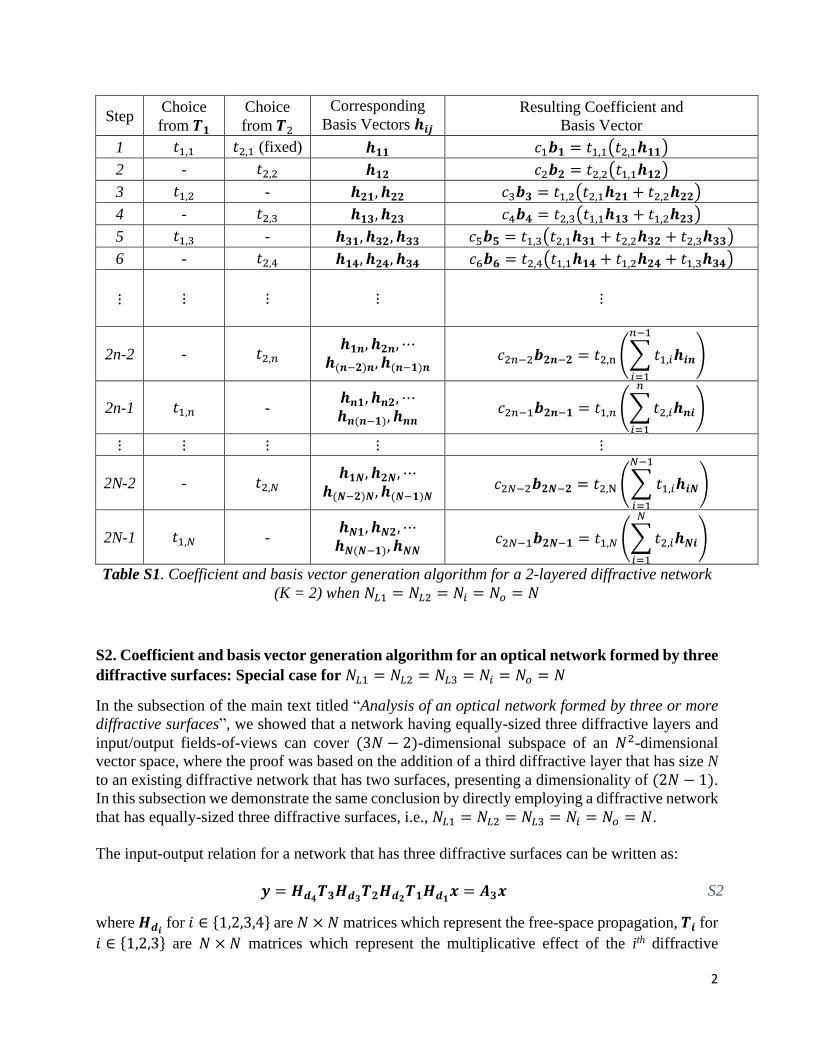
2

Step Choice

from 𝑻𝟏

Choice

from 𝑻2

Corresponding

Basis Vectors 𝒉𝒊𝒋 Resulting Coefficient and

Basis Vector

1 𝑡1,1 𝑡2,1 (fixed) 𝒉𝟏𝟏 𝑐1𝒃𝟏 = 𝑡1,1(𝑡2,1𝒉𝟏𝟏)

2 - 𝑡2,2 𝒉𝟏𝟐 𝑐2𝒃𝟐 = 𝑡2,2(𝑡1,1𝒉𝟏𝟐)

3 𝑡1,2 - 𝒉𝟐𝟏, 𝒉𝟐𝟐 𝑐3𝒃𝟑 = 𝑡1,2(𝑡2,1𝒉𝟐𝟏 + 𝑡2,2𝒉𝟐𝟐)

4 - 𝑡2,3 𝒉𝟏𝟑, 𝒉𝟐𝟑 𝑐4𝒃𝟒 = 𝑡2,3(𝑡1,1𝒉𝟏𝟑 + 𝑡1,2𝒉𝟐𝟑)

5 𝑡1,3 - 𝒉𝟑𝟏, 𝒉𝟑𝟐, 𝒉𝟑𝟑 𝑐5𝒃𝟓 = 𝑡1,3(𝑡2,1𝒉𝟑𝟏 + 𝑡2,2𝒉𝟑𝟐 + 𝑡2,3𝒉𝟑𝟑)

6 - 𝑡2,4 𝒉𝟏𝟒, 𝒉𝟐𝟒, 𝒉𝟑𝟒 𝑐6𝒃𝟔 = 𝑡2,4(𝑡1,1𝒉𝟏𝟒 + 𝑡1,2𝒉𝟐𝟒 + 𝑡1,3𝒉𝟑𝟒)

⋮

⋮ ⋮ ⋮ ⋮

2n-2 - 𝑡2,𝑛 𝒉𝟏𝒏, 𝒉𝟐𝒏, ⋯

𝒉(𝒏−𝟐)𝒏, 𝒉(𝒏−𝟏)𝒏 𝑐2𝑛−2𝒃𝟐𝒏−𝟐 = 𝑡2,n (∑ 𝑡1,𝑖𝒉𝒊𝒏

𝑛−1

𝑖=1

)

2n-1 𝑡1,𝑛 - 𝒉𝒏𝟏, 𝒉𝒏𝟐, ⋯

𝒉𝒏(𝒏−𝟏), 𝒉𝒏𝒏 𝑐2𝑛−1𝒃𝟐𝒏−𝟏 = 𝑡1,𝑛 (∑𝑡2,𝑖𝒉𝒏𝒊

𝑛

𝑖=1

)

⋮ ⋮ ⋮ ⋮ ⋮

2N-2 - 𝑡2,𝑁 𝒉𝟏𝑵, 𝒉𝟐𝑵, ⋯

𝒉(𝑵−𝟐)𝑵, 𝒉(𝑵−𝟏)𝑵 𝑐2𝑁−2𝒃𝟐𝑵−𝟐 = 𝑡2,N (∑ 𝑡1,𝑖𝒉𝒊𝑵

𝑁−1

𝑖=1

)

2N-1 𝑡1,𝑁 - 𝒉𝑵𝟏, 𝒉𝑵𝟐, ⋯

𝒉𝑵(𝑵−𝟏), 𝒉𝑵𝑵 𝑐2𝑁−1𝒃𝟐𝑵−𝟏 = 𝑡1,𝑁 (∑𝑡2,𝑖𝒉𝑵𝒊

𝑁

𝑖=1

)

Table S1. Coefficient and basis vector generation algorithm for a 2-layered diffractive network

(K = 2) when 𝑁𝐿1 = 𝑁𝐿2 = 𝑁𝑖 = 𝑁𝑜 = 𝑁

S2. Coefficient and basis vector generation algorithm for an optical network formed by three

diffractive surfaces: Special case for 𝑁𝐿1 = 𝑁𝐿2 = 𝑁𝐿3 = 𝑁𝑖 = 𝑁𝑜 = 𝑁

In the subsection of the main text titled “Analysis of an optical network formed by three or more

diffractive surfaces”, we showed that a network having equally-sized three diffractive layers and

input/output fields-of-views can cover (3𝑁 − 2)-dimensional subspace of an 𝑁2-dimensional

vector space, where the proof was based on the addition of a third diffractive layer that has size N

to an existing diffractive network that has two surfaces, presenting a dimensionality of (2𝑁 − 1).

In this subsection we demonstrate the same conclusion by directly employing a diffractive network

that has equally-sized three diffractive surfaces, i.e., 𝑁𝐿1 = 𝑁𝐿2 = 𝑁𝐿3 = 𝑁𝑖 = 𝑁𝑜 = 𝑁.

The input-output relation for a network that has three diffractive surfaces can be written as:

where 𝑯𝒅𝒊 for 𝑖 ∈ {1,2,3,4} are 𝑁 × 𝑁 matrices which represent the free-space propagation, 𝑻𝒊 for

𝑖 ∈ {1,2,3} are 𝑁 × 𝑁 matrices which represent the multiplicative effect of the ith diffractive

𝒚 = 𝑯𝒅𝟒𝑻𝟑𝑯𝒅𝟑

𝑻𝟐𝑯𝒅𝟐𝑻𝟏𝑯𝒅𝟏

𝒙 = 𝑨𝟑𝒙 S2

3

surface, and 𝒙 and 𝒚 are length-N vectors which represent the input and output fields-of-view,

respectively. Details of these matrices and vectors can be found in “Theoretical analysis of the

information-processing capacity of diffractive surfaces” subsection of the main text. In this

subsection, we show that 𝑣𝑒𝑐(𝑨𝟑) = 𝒂𝟑 can be written as:

where 𝑐𝑖 and 𝒃𝒊 are an arbitrary complex-valued coefficient and the corresponding basis vector,

respectively. We first perform the vectorization of 𝑨𝟑 as:

In order to uncouple the transmittance and free-space propagation parts in Equation S4, we define

a matrix ��𝒅𝟐𝟑 having size 𝑁2 × 𝑁4 from 𝑯𝒅𝟐

𝑇 ⊗ 𝑯𝒅𝟑 as:

where 𝒓𝒊 is the 𝑖th row of 𝑯𝒅𝟐

𝑇 ⊗ 𝑯𝒅𝟑 and 𝟎 is an all-zero row vector with size 1 × 𝑁2. Therefore,

in each row of ��𝒅𝟐𝟑, there are 𝑁4 − 𝑁2 many zeros. Also, let 𝒕𝟏𝟐𝟑 be a size 𝑁4 × 1 vector that is

generated as:

where 𝑡𝑖 = (𝑻𝟏 ⊗ 𝑻3)[𝑖, 𝑖]. Then, Equation S4 can be written as:

where (𝑯𝒅𝟏

𝑇 ⊗ 𝑯𝒅𝟒)��𝒅𝟐𝟑

has rank 𝑁2 since both 𝑯𝒅𝟏

𝑇 ⊗ 𝑯𝒅𝟒 and ��𝒅𝟐𝟑

have rank 𝑁2.

There are also 𝑁3-many nonzero elements of 𝒕𝟏𝟐𝟑, each of which takes the form 𝑡𝑖𝑗𝑘 = 𝑡1,𝑖𝑡2,𝑗𝑡3,𝑘

for 𝑖, 𝑗, 𝑘 ∈ {1,2, … ,𝑁}. Therefore 𝒂𝟑 can be written in the form:

where, 𝒉𝒊𝒋𝒌 represents the corresponding column vector of (𝑯𝒅𝟏

𝑇 ⊗ 𝑯𝒅𝟒)��𝒅𝟐𝟑

. Analogous to the

2-layer case, all 𝑡𝑖𝑗𝑘 in Equation S8 cannot be chosen arbitrarily since it includes multiplicative

terms of 𝑡1,𝑖 , 𝑡2,𝑗 𝑎𝑛𝑑 𝑡3,𝑘. However, by extending the algorithm detailed in Section S1 for the

𝒂𝟑 = ∑ 𝑐𝑖𝒃𝒊

3𝑁−2

𝑖=1

S3

𝑣𝑒𝑐(𝑨𝟑) = 𝒂𝟑 = 𝑣𝑒𝑐(𝑯𝒅𝟒𝑻𝟑𝑯𝒅𝟑

𝑻𝟐𝑯𝒅𝟐𝑻𝟏𝑯𝒅𝟏

)

= (𝑯𝒅𝟏

𝑇 ⊗ 𝑯𝒅𝟒)(𝑻𝟏

𝑇 ⊗ 𝑻3)(𝑯𝒅𝟐

𝑇 ⊗ 𝑯𝒅𝟑)𝑣𝑒𝑐(𝑻𝟐)

= (𝑯𝒅𝟏

𝑇 ⊗ 𝑯𝒅𝟒)(𝑻𝟏 ⊗ 𝑻3)(𝑯𝒅𝟐

𝑇 ⊗ 𝑯𝒅𝟑)𝑣𝑒𝑐(𝑻𝟐)

S4

��𝒅𝟐𝟑=

[ 𝒓𝟏 𝟎 𝟎 ⋯ 𝟎𝟎 𝒓𝟐 𝟎 ⋯ 𝟎𝟎 𝟎 𝒓𝟑 ⋯ 𝟎⋮ ⋮ ⋮ ⋮ ⋮𝟎 𝟎 𝟎 ⋯ 𝒓𝑵𝟐]

S5

𝒕𝟏𝟐𝟑 = [

𝑡1𝑣𝑒𝑐(𝑻𝟐)

𝑡2𝑣𝑒𝑐(𝑻𝟐)⋮

𝑡𝑁2𝑣𝑒𝑐(𝑻𝟐)

]

S6

𝑣𝑒𝑐(𝑨𝟑) = 𝒂𝟑 = (𝑯𝒅𝟏

𝑇 ⊗ 𝑯𝒅𝟒)��𝒅𝟐𝟑

𝒕𝟏𝟐𝟑 S7

𝒂𝟑 = ∑ 𝑡𝑖𝑗𝑘𝒉𝒊𝒋𝒌

𝑖,𝑗,𝑘

S8

4

current 3-layered network case, we can show that 𝒂𝟑 can be formed as:

where 𝑐𝑖 and 𝒃𝒊 are generated by following an algorithm which is the counterpart of the layer and

neuron selection algorithm presented for the 2-layer case in Table 1 of the main text. Based on this

algorithm, we randomly select a diffractive layer and a neuron on that selected layer at each step

of the algorithm to form 𝑐𝑖 and 𝒃𝒊 in Equation S9. We also present a special case of this algorithm

in Table S2, where the layers are chosen in a regular, pre-determined order. By summing the used

𝒉𝒊𝒋𝒌 vectors in the 5th column of Table S2, it can be shown that 𝑁3-many coefficients and vectors

are used to generate the new coefficients. As a result, a set of 𝒂𝟑 vectors can be generated from a

(3𝑁 − 2)-dimensional subspace of 𝑁2-dimensional vector space. Also see Supplementary Section

S4.3 and Supplementary Figure S3 for further analyses on K=3 case.

Step Choice

from 𝑻𝟏

Choice

from 𝑻2

Choice

from 𝑻3

Resulting Coefficient and

Basis Vector

1 𝑡1,1 𝑡2,1

(fixed)

𝑡3,1

(fixed) 𝑐1𝒃𝟏 = 𝑡1,1(𝑡2,1𝑡3,1𝒉𝟏𝟏𝟏)

2 - - 𝑡3,2 𝑐2𝒃𝟐 = 𝑡3,2(𝑡1,1𝑡2,1𝒉𝟏𝟏𝟐)

3 - 𝑡2,2 - 𝑐3𝒃𝟑 = 𝑡2,2(𝑡1,1𝑡3,1𝒉𝟏𝟐𝟏 + 𝑡1,1𝑡3,2𝒉𝟏𝟐𝟐)

4 𝑡1,2 - - 𝑐4𝒃𝟒 = 𝑡1,2(𝑡2,1𝑡3,1𝒉𝟐𝟏𝟏 + 𝑡2,1𝑡3,2𝒉𝟐𝟏𝟐 + 𝑡2,2𝑡3,1𝒉𝟐𝟐𝟏

+ 𝑡2,2𝑡3,2𝒉𝟐𝟐𝟐)

5 - - 𝑡3,3 𝑐5𝒃𝟓 = 𝑡3,3(𝑡1,1𝑡2,1𝒉𝟏𝟏𝟑 + 𝑡1,1𝑡2,2𝒉𝟏𝟐𝟑 + 𝑡1,2𝑡2,1𝒉𝟐𝟏𝟑

+ 𝑡1,2𝑡2,2𝒉𝟐𝟐𝟑)

6 - 𝑡2,3 - 𝑐6𝒃𝟔 = 𝑡2,3(𝑡1,1𝑡3,1𝒉𝟏𝟑𝟏 + 𝑡1,1𝑡3,2𝒉𝟏𝟑𝟐 + 𝑡1,1𝑡3,3𝒉𝟏𝟑𝟑

+ 𝑡1,2𝑡3,1𝒉𝟐𝟑𝟏 + +𝑡1,2𝑡3,2𝒉𝟐𝟑𝟐 + 𝑡1,2𝑡3,3𝒉𝟐𝟑𝟑)

7 𝑡1,3 - -

𝑐7𝒃𝟕 = 𝑡1,3(𝑡2,1𝑡3,1𝒉𝟑𝟏𝟏 + 𝑡2,1𝑡3,2𝒉𝟑𝟏𝟐 + 𝑡2,1𝑡3,3𝒉𝟑𝟏𝟑

+ 𝑡2,2𝑡3,1𝒉𝟑𝟐𝟏 + 𝑡2,2𝑡3,2𝒉𝟑𝟐𝟐 + 𝑡2,2𝑡3,3𝒉𝟑𝟐𝟑

+ 𝑡2,3𝑡3,1𝒉𝟑𝟑𝟏 + 𝑡2,3𝑡3,2𝒉𝟑𝟑𝟐 + 𝑡2,3𝑡3,3𝒉𝟑𝟑𝟑)

⋮ ⋮ ⋮ ⋮ ⋮

3n-4 - - 𝑡3,𝑛 𝑐3𝑛−4𝒃𝟑𝒏−𝟒 = 𝑡3,𝑛 (∑ ∑ 𝑡1,𝑖𝑡2,𝑗𝒉𝒊𝒋𝒏

𝑛−1

𝑗=1

𝑛−1

𝑖=1

)

3n-3 - 𝑡2,𝑛 - 𝑐3𝑛−3𝒃𝟑𝒏−𝟑 = 𝑡2,𝑛 (∑ ∑ 𝑡1,𝑖𝑡3,𝑘𝒉𝒊𝒏𝒌

𝑛

𝑘=1

𝑛−1

𝑖=1

)

3n-2 𝑡1,𝑛 - - 𝑐3𝑛−2𝒃𝟑𝒏−𝟐 = 𝑡1,𝑛 (∑ ∑ 𝑡2,𝑗𝑡3,𝑘𝒉𝒏𝒋𝒌

𝑛

𝑘=1

𝑛

𝑗=1

)

⋮ ⋮ ⋮ ⋮ ⋮

𝒂𝟑 = ∑ 𝑐𝑖𝒃𝒊

3𝑁−2

𝑖=1

S9

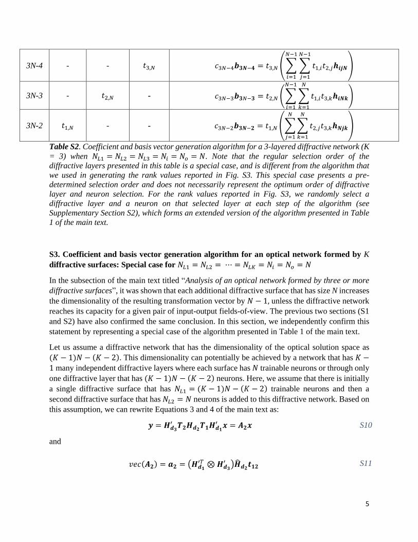
5

3N-4 - - 𝑡3,𝑁 𝑐3𝑁−4𝒃𝟑𝑵−𝟒 = 𝑡3,𝑁 (∑ ∑ 𝑡1,𝑖𝑡2,𝑗𝒉𝒊𝒋𝑵

𝑁−1

𝑗=1

𝑁−1

𝑖=1

)

3N-3 - 𝑡2,𝑁 - 𝑐3𝑁−3𝒃𝟑𝑁−𝟑 = 𝑡2,𝑁 (∑ ∑ 𝑡1,𝑖𝑡3,𝑘𝒉𝒊𝑵𝒌

𝑁

𝑘=1

𝑁−1

𝑖=1

)

3N-2 𝑡1,𝑁 - - 𝑐3𝑁−2𝒃𝟑𝑵−𝟐 = 𝑡1,𝑁 (∑ ∑ 𝑡2,𝑗𝑡3,𝑘𝒉𝑵𝒋𝒌

𝑁

𝑘=1

𝑁

𝑗=1

)

Table S2. Coefficient and basis vector generation algorithm for a 3-layered diffractive network (K

= 3) when 𝑁𝐿1 = 𝑁𝐿2 = 𝑁𝐿3 = 𝑁𝑖 = 𝑁𝑜 = 𝑁. Note that the regular selection order of the

diffractive layers presented in this table is a special case, and is different from the algorithm that

we used in generating the rank values reported in Fig. S3. This special case presents a pre-

determined selection order and does not necessarily represent the optimum order of diffractive

layer and neuron selection. For the rank values reported in Fig. S3, we randomly select a

diffractive layer and a neuron on that selected layer at each step of the algorithm (see

Supplementary Section S2), which forms an extended version of the algorithm presented in Table

1 of the main text.

S3. Coefficient and basis vector generation algorithm for an optical network formed by K

diffractive surfaces: Special case for 𝑁𝐿1 = 𝑁𝐿2 = ⋯ = 𝑁𝐿𝐾 = 𝑁𝑖 = 𝑁𝑜 = 𝑁

In the subsection of the main text titled “Analysis of an optical network formed by three or more

diffractive surfaces”, it was shown that each additional diffractive surface that has size N increases

the dimensionality of the resulting transformation vector by 𝑁 − 1, unless the diffractive network

reaches its capacity for a given pair of input-output fields-of-view. The previous two sections (S1

and S2) have also confirmed the same conclusion. In this section, we independently confirm this

statement by representing a special case of the algorithm presented in Table 1 of the main text.

Let us assume a diffractive network that has the dimensionality of the optical solution space as

(𝐾 − 1)𝑁 − (𝐾 − 2). This dimensionality can potentially be achieved by a network that has 𝐾 −

1 many independent diffractive layers where each surface has 𝑁 trainable neurons or through only

one diffractive layer that has (𝐾 − 1)𝑁 − (𝐾 − 2) neurons. Here, we assume that there is initially

a single diffractive surface that has 𝑁𝐿1 = (𝐾 − 1)𝑁 − (𝐾 − 2) trainable neurons and then a

second diffractive surface that has 𝑁𝐿2 = 𝑁 neurons is added to this diffractive network. Based on

this assumption, we can rewrite Equations 3 and 4 of the main text as:

and

𝒚 = 𝑯𝒅𝟑

′ 𝑻𝟐𝑯𝒅𝟐𝑻𝟏𝑯𝒅𝟏

′ 𝒙 = 𝑨𝟐𝒙 S10

𝑣𝑒𝑐(𝑨𝟐) = 𝒂𝟐 = (𝑯𝒅𝟏

′𝑇 ⊗ 𝑯𝒅𝟑

′ )��𝒅𝟐𝒕𝟏𝟐 S11

6

where, in this case, 𝑁𝐿1 = (𝐾 − 1)𝑁 − (𝐾 − 2) and 𝑁𝐿2 = 𝑁. Therefore, 𝒂𝟐 can be written as:

where 𝒉𝒊𝒋 is the corresponding column vector of (𝑯𝒅𝟏

′𝑇 ⊗ 𝑯𝒅𝟑

′ )��𝒅𝟐 which has rank 𝑁2 and 𝑡𝑖𝑗 =

𝑡1,𝑖𝑡2,𝑗, where 𝑡1,𝑖 and 𝑡2,𝑗 are the trainable complex-valued transmission coefficients of the 𝑖th

neuron of the 1st diffractive surface and the 𝑗th neuron of the 2nd diffractive surface, respectively,

for 𝑖 ∈ {1,2, … , (𝐾 − 1)𝑁 − (𝐾 − 2)} and 𝑗 ∈ {1,2, … , 𝑁}. Hence, we can show that 𝒂𝟐 can be

written as:

where 𝑐𝑖 and 𝒃𝒊 are an arbitrary complex-valued coefficient and the corresponding basis vector,

respectively. The algorithm that we use here is a special case of the algorithm given in the

subsection of the main text titled “Coefficient and basis vector generation for an optical network

formed by two diffractive surfaces” for the chunk partition 𝑛1 = 𝑛3 = ⋯ = 𝑛2𝑖−1 = ⋯ = 𝑛𝑠−1 =1 and 𝑛2 = 𝑛4 = ⋯ = 𝑛2𝑖 = ⋯ = 𝑛𝑠 = 𝐾. That is, after choosing one coefficient from 𝑡1,𝑖 and

𝑡2,𝑗 at the initialization step, we choose one coefficient from 𝑡2,𝑗 in the second step and one

coefficient from 𝑡1,𝑖 in each of the following K steps. In each step, we use the previously chosen

coefficients and the corresponding 𝒉𝒊𝒋 vectors in order to create the next basis vector. Then, this

procedure continues until all the coefficients have been used.

We summarized these steps of the coefficient and basis generation algorithm in Table S3, in the

next page. It can be shown that, all 𝑁[(𝐾 − 1)𝑁 − (𝐾 − 2)] nonzero coefficients (𝑡𝑖𝑗’s) are used

to generate 𝐾𝑁 − (𝐾 − 1) basis vectors. This analysis confirms that if there are (𝐾 − 1)𝑁 −(𝐾 − 2) neurons in a single layered network, the addition of a second diffractive layer with N

independent neurons can expand the dimensionality of the possible input-output transformations

by 𝑁 − 1, assuming the capacity limit (𝑁2) has not been reached.

𝒂𝟐 = ∑𝑡𝑖𝑗𝒉𝒊𝒋

𝑖,𝑗

, S12

𝒂𝟐 = ∑ 𝑐𝑖𝒃𝒊

𝐾𝑁−(𝐾−1)

𝑖=1

,

S13

7

Table S3. Coefficient and basis vector generation algorithm for a 2-layered diffractive network

when 𝑁𝐿1 = (𝐾 − 1)𝑁 − (𝐾 − 2) 𝑎𝑛𝑑 𝑁𝐿2 = 𝑁𝑖 = 𝑁𝑜 = 𝑁

Step Choice from 𝑻𝟏 Choice from 𝑻2 Resulting Coefficient and

Basis Vector

1 𝑡1,1 𝑡2,1 (fixed) 𝑐1𝒃𝟏 = 𝑡1,1(𝑡2,1𝒉𝟏𝟏)

2 - 𝑡2,2 𝑐2𝒃𝟐 = 𝑡2,2(𝑡1,1𝒉𝟏𝟐)

3 𝑡1,2 - 𝑐𝑖+1𝒃𝒊+𝟏 = 𝑡1,𝑖(𝑡2,1𝒉𝒊𝟏 + 𝑡2,2𝒉𝒊𝟐) ,

for

𝑖 ∈ {2,3, … , 𝐾}

4 𝑡1,3 -

⋮ ⋮ ⋮

K+1 𝑡1,𝐾 -

K+2 - 𝑡2,3 𝑐𝐾+2𝒃𝐾+𝟐 = 𝑡2,3 ( ∑𝑡1,𝑖𝒉𝒊𝟏

𝐾

𝑖=2

)

K+3 𝑡1,𝐾+1 - 𝑐𝑖+2𝒃𝒊+𝟐 = 𝑡1,𝑖(𝑡2,1𝒉𝒊𝟏 + 𝑡2,2𝒉𝒊𝟐 + 𝑡2,3𝒉𝒊𝟑) ,

for

𝑖 ∈ {𝐾 + 1,𝐾 + 2,… ,2𝐾 − 1}

K+4 𝑡1,𝐾+2 -

⋮ ⋮ ⋮

2K+1 𝑡1,2𝐾−1 -

⋮ ⋮ ⋮ ⋮

qK+2 - 𝑡2,𝑞+2 𝑐𝑞𝐾+2𝒃𝒒𝑲+𝟐 = 𝑡2,𝑞+2 ( ∑ 𝑡1,𝑖𝒉𝒊(𝒒+𝟐)

𝑞𝐾−(𝑞−1)

𝑖=1

)

qK+3 𝑡1,𝑞(𝐾−1)+2 -

𝑐𝑖+1𝒃𝒊+𝟏 = 𝑡1,𝑖−𝑞 ( ∑ 𝑡2,𝑗𝒉(𝒊−𝒒)𝒋

𝑞+2

𝑗=1

) ,

for

𝑖 ∈ {𝑞𝐾 + 2, 𝑞𝐾 + 3,… , 𝑞𝐾 + 𝐾}

qK+4 𝑡1,𝑞(𝐾−1)+3 -

⋮ ⋮ ⋮

(q+1)K+1 𝑡1,(𝑞+1)𝐾−𝑞 -

⋮ ⋮ ⋮ ⋮

(N-2)K+2 - 𝑡2,𝑁 𝑐(𝑁−2)𝐾+2𝒃(𝑵−𝟐)𝑲+𝟐 = 𝑡2,𝑁 ( ∑ 𝑡1,𝑖𝒉𝒊𝑵

(𝑁−2)𝐾−(𝑁−1)

𝑖=1

)

(N-2)K+3 𝑡1,(𝑁−2)(𝐾−1)+2 -

𝑐𝑖+𝑁−1𝒃𝒊+𝑵−𝟏 = 𝑡1,𝑖 ( ∑𝑡2,𝑗𝒉𝒊𝒋

𝑁

𝑗=1

) ,

for

𝑖 ∈ {(𝑁 − 2)(𝐾 − 1) + 2, (𝑁 − 2)(𝐾 − 1) + 3,… , (𝑁− 1)𝐾 − (𝑁 − 2)}

(N-2)K+4 𝑡1,(𝑁−2)(𝐾−1)+3 -

⋮ ⋮ ⋮

KN-(K-1) 𝑡1,(𝑁−1)𝐾−(𝑁−2) -

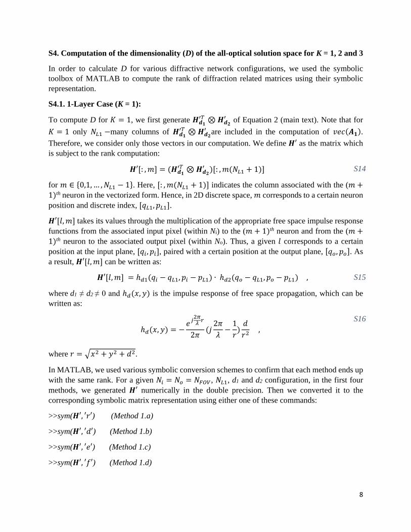
8

S4. Computation of the dimensionality (D) of the all-optical solution space for K = 1, 2 and 3

In order to calculate D for various diffractive network configurations, we used the symbolic

toolbox of MATLAB to compute the rank of diffraction related matrices using their symbolic

representation.

S4.1. 1-Layer Case (K = 1):

To compute D for 𝐾 = 1, we first generate 𝑯𝒅𝟏

′𝑇 ⊗ 𝑯𝒅𝟐

′ of Equation 2 (main text). Note that for

𝐾 = 1 only 𝑁𝐿1 −many columns of 𝑯𝒅𝟏

′𝑇 ⊗ 𝑯𝒅𝟐

′ are included in the computation of 𝑣𝑒𝑐(𝑨𝟏).

Therefore, we consider only those vectors in our computation. We define 𝑯′ as the matrix which

is subject to the rank computation:

for 𝑚 ∈ {0,1, … ,𝑁𝐿1 − 1}. Here, [: , 𝑚(𝑁𝐿1 + 1)] indicates the column associated with the (𝑚 +

1)th neuron in the vectorized form. Hence, in 2D discrete space, 𝑚 corresponds to a certain neuron

position and discrete index, [𝑞𝐿1, 𝑝𝐿1].

𝑯′[𝑙,𝑚] takes its values through the multiplication of the appropriate free space impulse response

functions from the associated input pixel (within Ni) to the (𝑚 + 1)th neuron and from the (𝑚 +

1)th neuron to the associated output pixel (within No). Thus, a given 𝑙 corresponds to a certain

position at the input plane, [𝑞𝑖 , 𝑝𝑖], paired with a certain position at the output plane, [𝑞𝑜, 𝑝𝑜]. As

a result, 𝑯′[𝑙,𝑚] can be written as:

where d1 ≠ d2 ≠ 0 and ℎ𝑑(𝑥, 𝑦) is the impulse response of free space propagation, which can be

written as:

where 𝑟 = √𝑥2 + 𝑦2 + 𝑑2.

In MATLAB, we used various symbolic conversion schemes to confirm that each method ends up

with the same rank. For a given 𝑁𝑖 = 𝑁𝑜 = 𝑁𝐹𝑂𝑉, 𝑁𝐿1, d1 and d2 configuration, in the first four

methods, we generated 𝑯′ numerically in the double precision. Then we converted it to the

corresponding symbolic matrix representation using either one of these commands:

>>sym(𝑯′, ′𝑟′) (Method 1.a)

>>sym(𝑯′, ′𝑑′) (Method 1.b)

>>sym(𝑯′, ′𝑒′) (Method 1.c)

>>sym(𝑯′, ′𝑓′) (Method 1.d)

𝑯′[: , 𝑚] = (𝑯𝒅𝟏

′𝑇 ⊗ 𝑯𝒅𝟐

′ )[: ,𝑚(𝑁𝐿1 + 1)] S14

𝑯′[𝑙,𝑚] = ℎ𝑑1(𝑞𝑖 − 𝑞𝐿1, 𝑝𝑖 − 𝑝𝐿1) ∙ ℎ𝑑2(𝑞𝑜 − 𝑞𝐿1, 𝑝𝑜 − 𝑝𝐿1) , S15

ℎ𝑑(𝑥, 𝑦) = −𝑒𝑗

2𝜋𝜆

𝑟

2𝜋(𝑗

2𝜋

𝜆−

1

𝑟)

𝑑

𝑟2 ,

S16

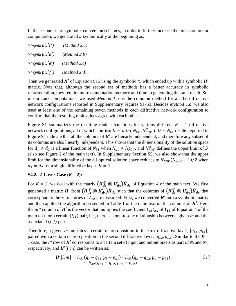
9

In the second set of symbolic conversion schemes, in order to further increase the precision in our

computation, we generated 𝜋 symbolically at the beginning as:

>>sym(𝑝𝑖, ′𝑟′) (Method 2.a)

>>sym(𝑝𝑖, ′𝑑′) (Method 2.b)

>>sym(𝑝𝑖, ′𝑒′) (Method 2.c)

>>sym(𝑝𝑖, ′𝑓′) (Method 2.d)

Then we generated 𝑯′ of Equation S15 using the symbolic 𝜋, which ended up with a symbolic 𝑯′ matrix. Note that, although the second set of methods has a better accuracy in symbolic

representation, they require more computation memory and time in generating the rank result. So,

in our rank computations, we used Method 1.a as the common method for all the diffractive

network configurations reported in Supplementary Figures S1-S3. Besides Method 1.a, we also

used at least one of the remaining seven methods in each diffractive network configuration to

confirm that the resulting rank values agree with each other.

Figure S1 summarizes the resulting rank calculations for various different K = 1 diffractive

network configurations, all of which confirm 𝐷 = 𝑚𝑖𝑛( 𝑁𝐿1 , 𝑁𝐹𝑂𝑉2 ). 𝐷 = 𝑁𝐿1 results reported in

Figure S1 indicate that all the columns of 𝑯′ are linearly independent, and therefore any subset of

its columns are also linearly independent. This shows that the dimensionality of the solution space

for 𝑑1 ≠ 𝑑2 is a linear function of 𝑁𝐿1 when 𝑁𝐿1 ≤ 𝑁𝐹𝑂𝑉2 , and 𝑁𝐹𝑂𝑉

2 defines the upper limit of 𝐷

(also see Figure 2 of the main text). In Supplementary Section S5, we also show that the upper

limit for the dimensionality of the all-optical solution space reduces to 𝑁𝐹𝑂𝑉(𝑁𝐹𝑂𝑉 + 1) 2⁄ when

𝑑1 = 𝑑2 for a single diffractive layer, 𝐾 = 1.

S4.2. 2-Layer Case (K = 2):

For K = 2, we deal with the matrix (𝑯𝒅𝟏

′𝑇 ⊗ 𝑯𝒅𝟑

′ )��𝒅𝟐 of Equation 4 of the main text. We first

generated a matrix 𝑯′ from (𝑯𝒅𝟏

′𝑇 ⊗ 𝑯𝒅𝟑

′ )��𝒅𝟐 such that the columns of (𝑯𝒅𝟏

′𝑇 ⊗ 𝑯𝒅𝟑

′ )��𝒅𝟐 that

correspond to the zero entries of 𝒕𝟏𝟐 are discarded. First, we converted 𝑯′ into a symbolic matrix

and then applied the algorithm presented in Table 1 of the main text on the columns of 𝑯′. Here

the 𝑚th column of 𝑯′ is the vector that multiplies the coefficient 𝑡1,𝑖𝑡2,𝑗 of 𝒕𝟏𝟐 of Equation 4 of the

main text for a certain (𝑖, 𝑗) pair, i.e., there is a one-to-one relationship between a given 𝑚 and the

associated (𝑖, 𝑗) pair.

Therefore, a given 𝑚 indicates a certain neuron position in the first diffractive layer, [𝑞𝐿1, 𝑝𝐿1],

paired with a certain neuron position in the second diffractive layer, [𝑞𝐿2, 𝑝𝐿2]. Similar to the K =

1 case, the lth row of 𝑯′ corresponds to a certain set of input and output pixels as part of Ni and No,

respectively, and 𝑯′[𝑙,𝑚] can be written as:

𝑯′[𝑙,𝑚] = ℎ𝑑1(𝑞𝑖 − 𝑞𝐿1, 𝑝𝑖 − 𝑝𝐿1) ∙ ℎ𝑑3(𝑞𝑜 − 𝑞𝐿2, 𝑝𝑜 − 𝑝𝐿2)

∙ ℎ𝑑2(𝑞𝐿1 − 𝑞𝐿2, 𝑝𝐿1 − 𝑝𝐿2)

S17

10

After generating 𝑯′ based on Equation S17, we converted it into the symbolic matrix

representation as described earlier for the 1-layer case, K = 1. Then, we applied the algorithm

presented in Table 1 of the main text to generate the basis vectors and their coefficients. Note that,

for each diffractive network configuration that we selected, we independently ran the same

algorithm three times with different random initializations, random selection of the neurons and

random generation of complex-valued transmission coefficients. In all of the rank results that are

reported in Figure S2, these repeated simulations agreed with each other and gave the same rank,

confirming 𝐷 = 𝑚𝑖𝑛( 𝑁𝐿1 + 𝑁𝐿2 − 1,𝑁𝐹𝑂𝑉2 ). Also note that, unlike the d1 = d2 case for K = 1

(Section S5), different combinations of d1, d2 and d3 values for K = 2 do not change the results or

the upper bound of D, as also confirmed in Figure S2.

S4.3. 3-Layer Case (K = 3):

For K = 3 case, we start with (𝑯𝒅𝟏

𝑇 ⊗ 𝑯𝒅𝟒)��𝒅𝟐𝟑

of Equation S7. Then, we generate the matrix 𝑯′

by discarding the columns of (𝑯𝒅𝟏

𝑇 ⊗ 𝑯𝒅𝟒)��𝒅𝟐𝟑

that correspond to the zero entries of 𝒕𝟏𝟐𝟑 of

Equation S7. Here, the 𝑚th column of 𝑯′ is the vector that multiplies the coefficient 𝑡1,𝑖𝑡2,𝑗𝑡3,𝑘 for

a certain (𝑖, 𝑗, 𝑘) triplet. Hence, there is a one-to-one relationship between a given m and the

pixel/neuron locations from the first, second and third diffractive layers, which are represented by

[𝑞𝐿1, 𝑝𝐿1], [𝑞𝐿2, 𝑝𝐿2] and [𝑞𝐿3, 𝑝𝐿3], respectively. Similar to the K = 1 and K = 2 cases discussed in

earlier sections, a given row, l, corresponds to a certain set of input (from Ni) and output (from No)

pixels, [𝑞𝑖 , 𝑝𝑖] and [𝑞𝑜, 𝑝𝑜], respectively. Accordingly, 𝑯′[𝑙,𝑚] can be written as:

Then, we applied a coefficient and basis generation algorithm that is similar to Table 1 of the main

text, where we randomly select the diffractive layer and the neuron in each step of the algorithm

to obtain the resulting coefficients and the basis vectors. Then we converted the resulting vectors

into their symbolic representations as discussed earlier for the K = 1 case and computed the rank

of the resulting symbolic matrix. For K = 3 the selection order of the 1st, 2nd and 3rd diffractive

layers in consecutive steps and the location/value of the chosen neuron at each step may affect the

computed rank. Especially, when 𝑁𝐿1 + 𝑁𝐿2 + 𝑁𝐿3 is close to 𝑁𝐹𝑂𝑉2 , the probability of repeatedly

achieving the upper-bound of the dimensionality of the solution space, i.e., 𝑚𝑖𝑛( 𝑁𝐿1 + 𝑁𝐿2 +

𝑁𝐿3 − 2,𝑁𝐹𝑂𝑉2 ), using random orders of selection decreases. On the other hand, when 𝑁𝐿1 +

𝑁𝐿2 + 𝑁𝐿3 is considerably larger than 𝑁𝐹𝑂𝑉2 , due to the additional degrees of freedom in the

diffractive system, the probability of repeatedly achieving the upper-bound of the dimensionality

using random orders of selection significantly increases. In Figure S3, we present the computed

ranks for different K=3 diffractive network configurations; for each one of these configurations

that we considered in our simulations, we obtained at least one random selection of the diffractive

layers and neurons that attained full rank, numerically confirming 𝐷 = 𝑚𝑖𝑛( 𝑁𝐿1 + 𝑁𝐿2 + 𝑁𝐿3 −

2,𝑁𝐹𝑂𝑉2 ).

𝑯′[𝑙,𝑚] = ℎ𝑑1(𝑞𝑖 − 𝑞𝐿1, 𝑝𝑖 − 𝑝𝐿1) ∙ ℎ𝑑4(𝑞𝑜 − 𝑞𝐿3, 𝑝𝑜 − 𝑝𝐿3)

∙ ℎ𝑑2(𝑞𝐿1 − 𝑞𝐿2, 𝑝𝐿1 − 𝑝𝐿2) ∙ ℎ𝑑3(𝑞𝐿2 − 𝑞𝐿3, 𝑝𝐿2 − 𝑝𝐿3)

S18

11

S5. The Upper Bound of the Dimensionality (D) of the Solution Space Reduces to

(𝑵𝑭𝑶𝑽𝟐 + 𝑵𝑭𝑶𝑽) 𝟐⁄ when 𝒅𝟏 = 𝒅𝟐 for 𝑲 = 𝟏

For K = 1 and the special case of 𝑑1 = 𝑑2 = 𝑑, we can rewrite 𝑯′[𝑙, 𝑚] given by Equation S15 as:

To quantify the reduction in rank due to 𝑑1 = 𝑑2, among 𝑁𝐹𝑂𝑉2 entries of 𝑯′′[: , 𝑚], let us first

consider the cases where (𝑞𝑖 , 𝑝𝑖) ≠ (𝑞𝑜, 𝑝𝑜). For a given neuron or 𝑚, assuming that (𝑞𝑖 , 𝑝𝑖) ≠

(𝑞𝑜, 𝑝𝑜), the number of different entries that can be produced by Equation S19 becomes 𝐶(𝑁𝐹𝑂𝑉2

),

where 𝐶(∙∙) indicates the combination operation and 𝑁𝐹𝑂𝑉 = 𝑁𝑖 = 𝑁𝑜. Stated differently, since

ℎ𝑑1 = ℎ𝑑2 the order of the selections from (𝑞𝑖 , 𝑝𝑖) and (𝑞𝑜, 𝑝𝑜) does not matter, making the

selection defined by a combination operation, i.e., 𝐶(𝑁𝐹𝑂𝑉2

). In addition to these combinatorial

entries, there are 𝑁𝐹𝑂𝑉 additional entries that represent (𝑞𝑖 , 𝑝𝑖) = (𝑞𝑜, 𝑝𝑜). Therefore, the total

number of unique entries in a column, 𝑯′′[: , 𝑚], becomes:

This analysis proves that, for K = 1, the upper limit of the dimensionality (D) of the all-optical

solution space for 𝑑1 = 𝑑2 reduces from 𝑁𝐹𝑂𝑉2 to (𝑁𝐹𝑂𝑉

2 + 𝑁𝐹𝑂𝑉) 2⁄ due to the fact that ℎ𝑑1 =

ℎ𝑑2 = ℎ𝑑 in Equation S19.

Note that, when 𝑑1 ≠ 𝑑2, we have ℎ𝑑1 ≠ ℎ𝑑2, which directly implies that the combination

operation in Equation S20 must be replaced with the permutation operation, 𝑃(∙∙), since the order

of selections from (𝑞𝑖 , 𝑝𝑖) and (𝑞𝑜, 𝑝𝑜) matters (see Equation S15). Therefore, when 𝑑1 ≠ 𝑑2, Equation S20 is replaced with:

which confirms our analyses in the main text, reported in the subsection “Analysis of a single

diffractive surface” as well as the results reported in Figure S1.

𝑯′′[𝑙,𝑚] = ℎ𝑑(𝑞𝑖 − 𝑞𝐿1, 𝑝𝑖 − 𝑝𝐿1) ℎ𝑑(𝑞𝑜 − 𝑞𝐿1, 𝑝𝑜 − 𝑝𝐿1). S19

𝐶 (

𝑁𝐹𝑂𝑉

2) + 𝑁𝐹𝑂𝑉 = (𝑁𝐹𝑂𝑉

2 + 𝑁𝐹𝑂𝑉) 2⁄ . S20

𝑃 (𝑁𝐹𝑂𝑉

2) + 𝑁𝐹𝑂𝑉 = 𝑁𝐹𝑂𝑉

2 S21

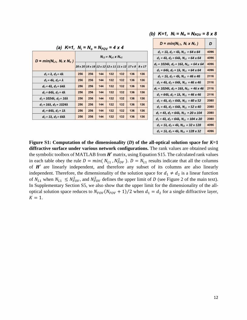
12

Figure S1: Computation of the dimensionality (D) of the all-optical solution space for K=1

diffractive surface under various network configurations. The rank values are obtained using

the symbolic toolbox of MATLAB from 𝑯′ matrix, using Equation S15. The calculated rank values

in each table obey the rule 𝐷 = 𝑚𝑖𝑛( 𝑁𝐿1 , 𝑁𝐹𝑂𝑉2 ). 𝐷 = 𝑁𝐿1 results indicate that all the columns

of 𝑯′ are linearly independent, and therefore any subset of its columns are also linearly

independent. Therefore, the dimensionality of the solution space for 𝑑1 ≠ 𝑑2 is a linear function

of 𝑁𝐿1 when 𝑁𝐿1 ≤ 𝑁𝐹𝑂𝑉2 , and 𝑁𝐹𝑂𝑉

2 defines the upper limit of 𝐷 (see Figure 2 of the main text).

In Supplementary Section S5, we also show that the upper limit for the dimensionality of the all-

optical solution space reduces to 𝑁𝐹𝑂𝑉(𝑁𝐹𝑂𝑉 + 1) 2⁄ when 𝑑1 = 𝑑2 for a single diffractive layer,

𝐾 = 1.

13

Figure S2: Computation of the dimensionality (D) of the all-optical solution space for K=2

diffractive surfaces under various network configurations. The rank values are obtained using

the symbolic toolbox of MATLAB from 𝑯′ matrix, based on Equation S17 and Table 1 of the

main text. Each result in the presented tables is confirmed through three independent runs of the

same algorithm with different random initializations, random selection of the neurons and random

generation of complex-valued transmission coefficients. All the presented rank results numerically

confirm 𝐷 = 𝑚𝑖𝑛( 𝑁𝐿1 + 𝑁𝐿2 − 1 , 𝑁𝐹𝑂𝑉2 ).

14

Figure S3: Computation of the dimensionality (D) of the all-optical solution space for K=3

diffractive surfaces under various network configurations. The rank values are obtained using

the symbolic toolbox of MATLAB from 𝑯′ matrix, based on Equation S18 and the algorithm

discussed in Section S2 (also see the supplementary text, Section S4.3, for details). The presented

results indicate that it is possible to obtain the maximum dimensionality of the solution space,

numerically confirming that 𝐷 = 𝑚𝑖𝑛( 𝑁𝐿1 + 𝑁𝐿2 + 𝑁𝐿3 − 2,𝑁𝐹𝑂𝑉2 ).

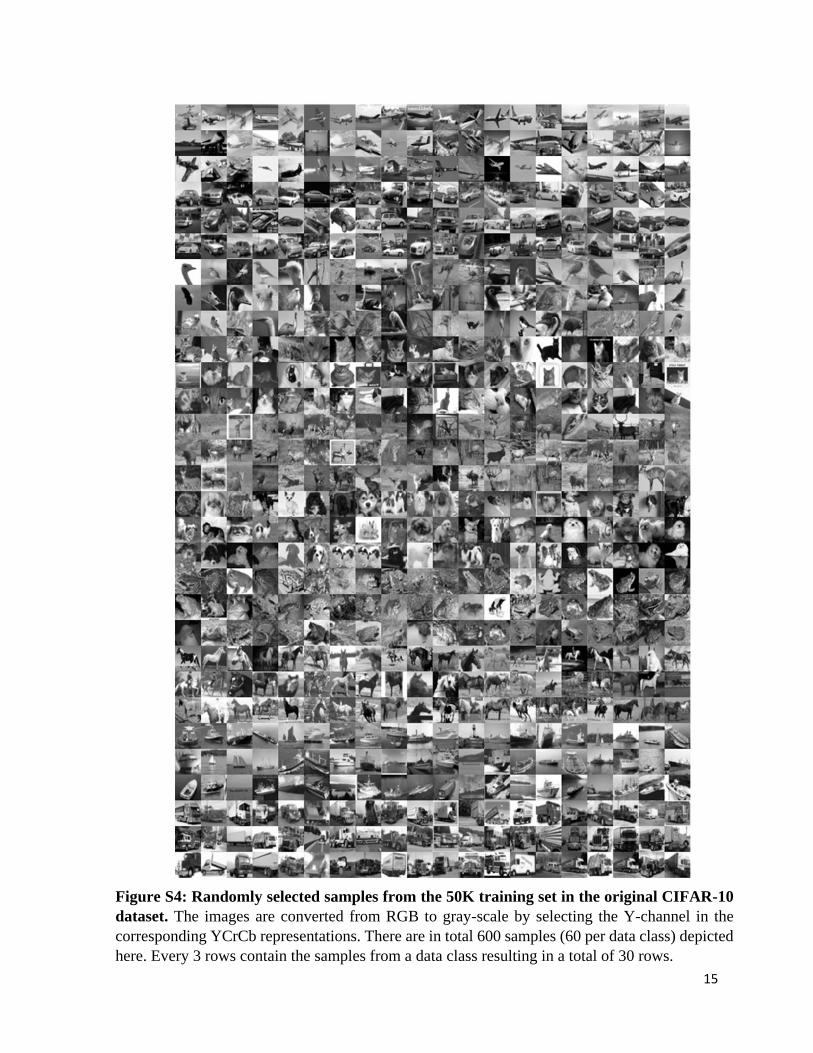
15

Figure S4: Randomly selected samples from the 50K training set in the original CIFAR-10

dataset. The images are converted from RGB to gray-scale by selecting the Y-channel in the

corresponding YCrCb representations. There are in total 600 samples (60 per data class) depicted

here. Every 3 rows contain the samples from a data class resulting in a total of 30 rows.

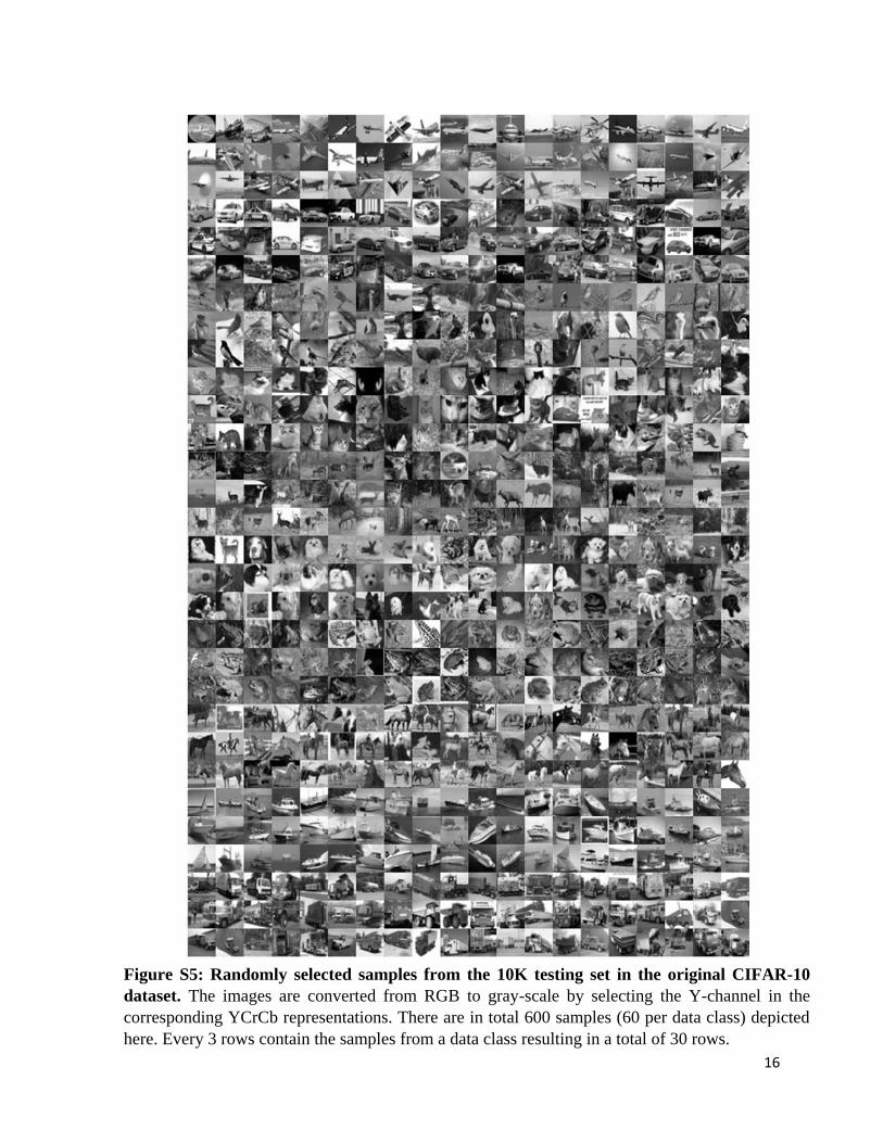
16

Figure S5: Randomly selected samples from the 10K testing set in the original CIFAR-10

dataset. The images are converted from RGB to gray-scale by selecting the Y-channel in the

corresponding YCrCb representations. There are in total 600 samples (60 per data class) depicted

here. Every 3 rows contain the samples from a data class resulting in a total of 30 rows.