article - Ibis bioinformatics

Chapter 13

Network Dynamics

Herbert M. Sauro

Abstract

Probably one of the most characteristic features of a living system is its continual propensity to change as itjuggles the demands of survival with the need to replicate. Internally these adjustments are manifest aschanges in metabolite, protein, and gene activities. Such changes have become increasingly obvious toexperimentalists, with the advent of high-throughput technologies. In this chapter we highlight some ofthe quantitative approaches used to rationalize the study of cellular dynamics. The chapter focusesattention on the analysis of quantitative models based on differential equations using biochemical controltheory. Basic pathway motifs are discussed, including straight chain, branched, and cyclic systems. Inaddition, some of the properties conferred by positive and negative feedback loops are discussed, particu-larly in relation to bistability and oscillatory dynamics.

Key words: Motifs, control analysis, stability, dynamic models.

1. Introduction

Probably, one of the most characteristic features of a living systemis its continual propensity to change even though it is also arguablythe one characteristic that, as molecular biologists, we oftenignore. Part of the reason for this neglect is the difficulty in makingtime-dependent quantitative measurements of proteins and othermolecules although that is rapidly changing with advances intechnology. The dynamics of cellular processes, and in particularcellular networks, is one of the defining attributes of the livingstate and deserves special attention.

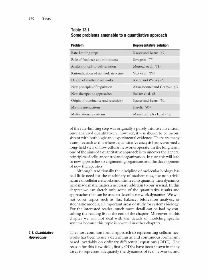
Before proceeding to the main discussion, it is worth brieflylisting the kinds of questions that can and have been answered by aquantitative approach (See Table 13.1). For example, the notion

Jason McDermott et al. (eds.), Computational Systems Biology, vol. 541ª Humana Press, a part of Springer Science+Business Media, LLC 2009DOI 10.1007/978-1-59745-243-4_13

269

of the rate-limiting step was originally a purely intuitive invention;once analyzed quantitatively, however, it was shown to be incon-sistent with both logic and experimental evidence. There are manyexamples such as this where a quantitative analysis has overturned along-held view of how cellular networks operate. In the long term,one of the aims of a quantitative approach is to uncover the generalprinciples of cellular control and organization. In turn this will leadto new approaches to engineering organisms and the developmentof new therapeutics.

Although traditionally the discipline of molecular biology hashad little need for the machinery of mathematics, the non-trivialnature of cellular networks and the need to quantify their dynamicshave made mathematics a necessary addition to our arsenal. In thischapter we can sketch only some of the quantitative results andapproaches that can be used to describe network dynamics. We willnot cover topics such as flux balance, bifurcation analysis, orstochastic models, all important areas of study for systems biology.For the interested reader, much more detail can be had by con-sulting the reading list at the end of the chapter. Moreover, in thischapter we will not deal with the details of modeling specificsystems because this topic is covered in other chapters.

1.1. Quantitative

Approaches

The most common formal approach to representing cellular net-works has been to use a deterministic and continuous formalism,based invariably on ordinary differential equations (ODE). Thereason for this is twofold, firstly ODEs have been shown in manycases to represent adequately the dynamics of real networks, and

Table 13.1Some problems amenable to a quantitative approach

Problem Representative solution

Rate-limiting steps Kacser and Burns (49)

Role of feedback and robustness Savageau (77)

Analysis of cell-to-cell variation Mettetal et al. (61)

Rationalization of network structure Voit et al. (87)

Design of synthetic networks Kaern and Weiss (51)

New principles of regulation Altan-Bonnet and Germain (1)

New therapeutic approaches Bakker et al. (5)

Origin of dominance and recessivity Kacser and Burns (50)

Missing interactions Ingolia (46)

Multistationary systems Many Examples Exist (52)

270 Sauro

secondly, there is a huge range of analytical results on the ODE-based models one can draw upon. Such analytical results arecrucial to enabling a deeper understanding of the networkunder study.

An alternative approach to describing cellular networks is touse a discrete, stochastic approach, based usually on the solution ofthe master equation via the Gillespie method (27,28). Thisapproach takes into account the fact that at the molecular level,species concentrations are whole numbers and change in discrete,integer amounts. In addition, changes in molecular amounts areassumed to be brought about by the inherent random nature ofmicroscopic molecular collisions. In principle, many researchersview the stochastic approach to be a superior representationbecause it directly attempts to describe the molecular milieu ofthe cellular space. However, the approach has two severe limita-tions, the first is that the method does not scale, that is, whensimulating large systems, particularly where the number of mole-cules is large (>200), it is computationally very expensive. Sec-ondly, there are few analytical results available to analyze stochasticmodels, which means that analysis is largely confined to numericalstudies from which it is difficult to generalize. One of the great andexciting challenges for the future is to develop the stochasticapproach to a point where it is as powerful a description as thecontinuous, deterministic approach. Without doubt, there is agrowing body of work, such as studies on measuring gene expres-sion in single cells, which depends very much on a stochasticrepresentation. Unfortunately, the theory required to interpretand analyze stochastic models is still immature though rapidlychanging (66, 78). The reader may consider the companion chap-ter by Resat et al. for the latest developments in stochasticdynamics.

In this chapter we will concentrate on some properties ofnetwork structures using a deterministic, continuous approach.

2. StoichiometricNetworks

The analysis of any biochemical network starts by considering thenetwork’s topology. This information is embodied in the stoichio-metry matrix, N (Note 1). In the following description we willfollow the standard formalism introduced by Reder (70). Thecolumns of the stoichiometry matrix correspond to the distinctchemical reactions in the network, the rows to the molecularspecies, one row per species. Thus the intersection of a row andcolumn in the matrix indicates whether a certain species takes partin a particular reaction or not, and, according to the sign of the

Network Dynamics 271

element, whether it is a reactant or product, and by the magnitude,the relative quantity of substance that takes part in that reaction.Stoichiometry thus concerns the relative mole amounts of chemi-cal species that react in a particular reaction; it does not concernitself with the rate of reaction.

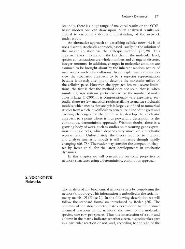
If a given network is composed of m molecular speciesinvolved in n reactions, then the stoichiometry matrix is an m �n matrix. Only those molecular species that evolve through thedynamics of the system are included in this count. Any source andsink species needed to sustain a steady state (non-equilibrium inthe thermodynamic sense) are set at a constant level and thereforedo not have corresponding entries in the stoichiometry matrix(Fig. 13.1).

2.1. The System

Equation

To fully characterize a system one also needs to consider thekinetics of the individual reactions as well as the network’s topol-ogy. Modeling the reactions by differential equations, we arrive ata system equation that involves both the stoichiometry matrix andthe rate vector, thus:

dS

dt¼ Nv; ½1�

where N is the m � n stoichiometry matrix and v is the n dimen-sional rate vector, whose ith component gives the rate of reaction ias a function of the species concentrations.

2.2. Conservation Laws In many models of real systems, there will be mass constraints onone or more sets of species. Such species are termed conservedmoieties (71). A recent review of conservation analysis, which alsohighlights the history of stoichiometric analysis, can be found in(73). In this section only the main results will be given.

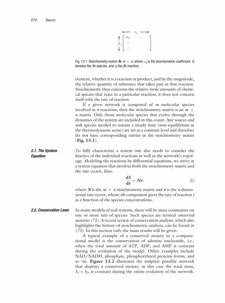
A typical example of a conserved moiety in a computa-tional model is the conservation of adenine nucleotide, i.e.,when the total amount of ATP, ADP, and AMP is constantduring the evolution of the model. Other examples includeNAD/NADH, phosphate, phosphorylated proteins forms, andso on. Figure 13.2 illustrates the simplest possible networkthat displays a conserved moiety; in this case the total mass,S1 + S2, is constant during the entire evolution of the network.

Si

vj⎡⎢⎣

αij ... .........

⎤⎥⎦

Fig. 13.1. Stoichiometry matrix: N: m � n, where �ij is the stoichiometric coefficient. Si

denotes the ith species, and vj the jth reaction.

272 Sauro

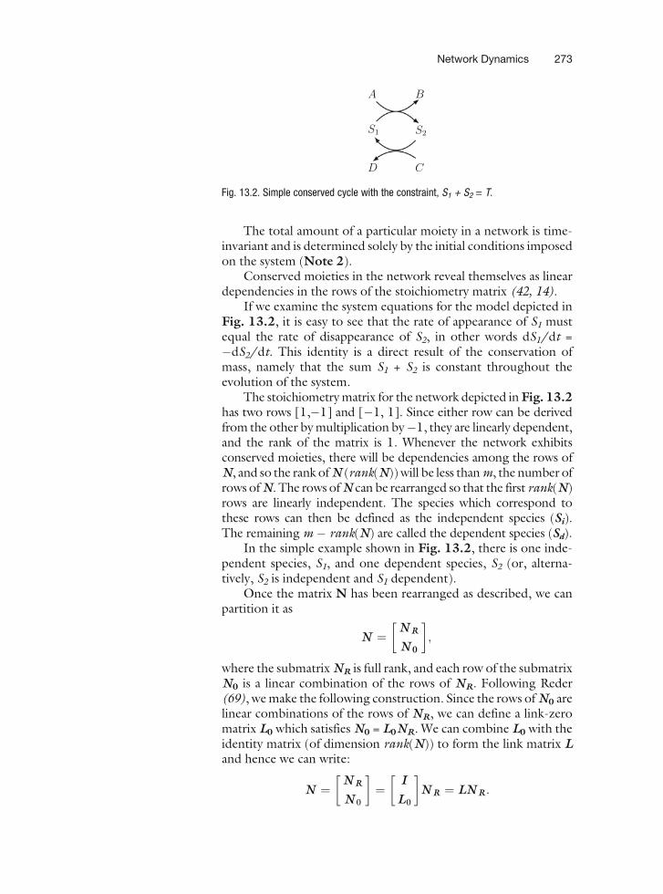
The total amount of a particular moiety in a network is time-invariant and is determined solely by the initial conditions imposedon the system (Note 2).

Conserved moieties in the network reveal themselves as lineardependencies in the rows of the stoichiometry matrix (42, 14).

If we examine the system equations for the model depicted inFig. 13.2, it is easy to see that the rate of appearance of S1 mustequal the rate of disappearance of S2, in other words dS1/dt =�dS2/dt. This identity is a direct result of the conservation ofmass, namely that the sum S1 + S2 is constant throughout theevolution of the system.

The stoichiometry matrix for the network depicted in Fig. 13.2has two rows [1,�1] and [�1, 1]. Since either row can be derivedfrom the other by multiplication by�1, they are linearly dependent,and the rank of the matrix is 1. Whenever the network exhibitsconserved moieties, there will be dependencies among the rows ofN, and so the rank of N (rank(N)) will be less than m, the number ofrows of N. The rows of N can be rearranged so that the first rank(N)rows are linearly independent. The species which correspond tothese rows can then be defined as the independent species (Si).The remaining m � rank(N) are called the dependent species (Sd).

In the simple example shown in Fig. 13.2, there is one inde-pendent species, S1, and one dependent species, S2 (or, alterna-tively, S2 is independent and S1 dependent).

Once the matrix N has been rearranged as described, we canpartition it as

N ¼N R

N 0

� �;

where the submatrix NR is full rank, and each row of the submatrixN0 is a linear combination of the rows of NR. Following Reder(69), we make the following construction. Since the rows of N0 arelinear combinations of the rows of NR, we can define a link-zeromatrix L0 which satisfies N0 = L0NR. We can combine L0 with theidentity matrix (of dimension rank(N)) to form the link matrix Land hence we can write:

N ¼N R

N 0

� �¼

I

L0

� �N R ¼ LN R:

S1 S2

A B

D C

Fig. 13.2. Simple conserved cycle with the constraint, S1 + S2 = T.


By partitioning the stoichiometry matrix into dependent andindependent sets, we also partition the system equation. The fullsystem equation, which describes the dynamics of the network, isthus:

I

L0

� �N Rv ¼ dS

dt¼

dSi=dt

dSd=dt

� �;

where the terms dSi/dt and dSd/dt refer to the independent anddependent rates of change, respectively. From the above equation,it can be shown that the relationship between the dependent andthe independent species is given by: Sd(t) � Sd(0) ¼ L0 [Si(t) �Si(0)] for all time t. Introducing the constant vector T ¼ Sd(0) �L0Si(0), and recalling that S ¼ (Si, Sd), we can introduce G ¼[�L0, I], and write the vector T concisely as

GS ¼ T :

G is called the conservation matrix.In the example shown in Fig. 13.2, the conservation matrix G

can be shown to be

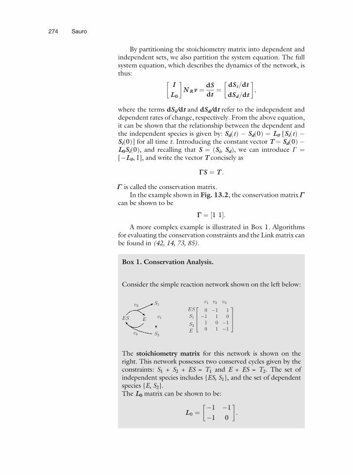
G ¼ 1 1½ �:A more complex example is illustrated in Box 1. Algorithms

for evaluating the conservation constraints and the Link matrix canbe found in (42, 14, 73, 85).

Box 1. Conservation Analysis.

Consider the simple reaction network shown on the left below:

v2

v3

ES E

S1

S2

v1

ES

S1

S2

E

v1 v2 v3⎡⎢⎢⎣

0 −1 1−1 1 0

1 0 −10 1 −1

⎤⎥⎥⎦

The stoichiometry matrix for this network is shown on theright. This network possesses two conserved cycles given by theconstraints: S1 + S2 + ES = T1 and E + ES = T2. The set ofindependent species includes {ES, S1}, and the set of dependentspecies {E, S2}.The L0 matrix can be shown to be:

L0 ¼�1 �1

�1 0

� �:

274 Sauro

The complete set of equations for this model is therefore:

S2

E

� �¼�1 �1

�1 0

� �ES

S1

� �þ

T1

T2

� �

dES=dt

dS1=dt

� �¼

0 �1 1

�1 1 0

� � v1

v2

v3

264

375:

Note that even though there appears to be four variables in thissystem, there are in fact only two independent variables, {ES,S1}, and hence only two differential equations and two linearconstraints.

An excellent source of material related to the analysis of thestoichiometry matrix can be found in the text book by Heinrichand Schuster (37) and more recently (53).

3. BiochemicalControl Theory

The system Eq. [1] describes the time evolution of the network.This evolution can be characterized in three ways: thermodynamicequilibrium where all net flows are zero and no concentrationschange in time; steady state where net flows of mass traverse theboundaries of the network and no concentrations change in time;and finally the transient state where flows and concentrations areboth changing in time. Only the steady state and transients states areof real interest in biology. Steady states can be further characterizedas stable or unstable, which will be discussed in a later section.

The steady-state solution for a network is obtained by settingthe left-hand side of the system Eq. [1] to zero, Nv = 0, and solvingfor the concentrations. Consider the simplest possible model:

Xo ! S1 ! X1; ½2�

where we will assume that Xo and X1 are boundary species that donot change in time and that each reaction is governed by simplemass-action kinetics. With these assumptions we can write downthe system equation for the rate of change of S1 as:

dS1=dt ¼ k1Xo � k2S1:

We can solve for the transient behavior of this system by integratingthe system equation and setting an initial condition, S1(0) = Ao, to yield:

S1ðtÞ ¼ Aoe�k2t þ k1X0

k21� e�k2t� �

:


This equation describes how the concentration of S1 changes intime. The steady state can be determined either by letting t go toinfinity or by setting the system equation to zero and solving for S1;either way, the steady-state concentration of S1 can be shown to be:

S1 ¼k1X0

k2:

Although simple systems such as this can be solved analyticallyfor both the time course evolution and the steady state, the methodrapidly becomes unworkable for larger systems. The problembecomes particulary acute when, instead of simple mass-actionkinetics, we begin to use enzyme kinetic rate laws that introducenonlinearities into the equations. For all intent and purposes, ana-lytical solutions for biologically interesting systems are unattainable.Instead one must turn to numerical solutions; however, numericalsolutions are particular solutions, not general, which an analyticalapproach would yield. As a result, to obtain a thorough under-standing of a model, many numerical simulations may need to becarried out. In view of these limitations many researchers apply smallperturbation theory (linearization) around some operating point,usually the steady state. By analyzing the behavior of the systemusing small perturbations, only the linear modes of the model arestimulated and therefore the mathematics becomes tractable. This isa tried and tested approach that has been used extensively in manyfields, particularly engineering, to deal with systems where themathematics makes analysis difficult.

Probably, the first person to consider the linearization of bio-chemical models was Joseph Higgins at the University of Pennsylvaniain the 1950s. Higgins introduced the idea of a ‘‘reflection coefficient’’(40, 38), which described the relative change of one variable toanother for small perturbations. In his Ph.D. thesis, Higgins describesmany properties of the reflection coefficients and in later work, threegroups, Savageau (75, 77), Heinrich and Rapoport (36, 35), andKacser and Burns (9, 49) independently and simultaneously devel-oped this work into what is now called Metabolic Control Analysis orBiochemical Systems Theory. These developments extended Higgins’original ideas significantly and the formalism is now the theoreticalfoundation for describing deterministic, continuous models of bio-chemical networks. The theory has, in the past 20 years or so, beenfurther developed with the most recent important advances by Ingalls(45) and Rao (68). In this chapter we will call this approach Biochem-ical Control Theory, or BCT.

3.1. Linear Perturbation

Analysis

3.1.1. Elementary

Processes

The fundamental unit in biological networks is the chemical trans-formation. Such transformations vary, ranging from simple bind-ing processes, transport processes, to more elaborate aggregatedkinetics such as Michaelis-Menten and complex cooperativekinetics.

276 Sauro

Traditionally, chemical transformations are described using arate law. For example, the rate law for a simple irreversible Michae-lis-Menten reaction is often given as

v ¼ V max S

Kmþ S; ½3�

where S is the substrate and the Vmax and Km kinetic constants.Such rate laws form the basis of larger pathway models.

A fundamental property of any rate law is the so-called kineticorder, sometimes also called the reaction order. In simple mass-action chemical kinetics, the kinetic order is the power to which aspecies is raised in the kinetic rate law. Reactions with zero-order,first-order, and second-order are the common types of reactionsfound in chemistry, and in each case the kinetic order is zero, one,and two, respectively. It is possible to generalize the kinetic orderas the scaled derivative of the reaction rate with respect to thespecies concentration, thus

Elasticity Coefficient: evS ¼

@v

@S

S

v¼ @ ln v

@ ln S� v%=S%:

When expressed this way, the kinetic order in biochemistry iscalled the elasticity coefficient. Applied to a simple mass-action ratelaw such as v = kS, we can see that ev

S ¼ 1. For a generalized mass-action law such as

v ¼ kY

Sni

i ;

the elasticity for the ith species is simply ni, that is, it equals thekinetic order. For aggregate rate laws such as the Michaelis-Men-ten rate law, the elasticity is more complex, for example, theelasticity for the rate law Eq. [3] is:

evS ¼

Km

S þKm:

This equation illustrates that the kinetic order, though a con-stant for simple rate laws, is a variable for complex rate laws. In thisparticular case, the elasticity approaches unity at low substrateconcentrations (first-order) and zero at high substrate concentra-tions (zero-order).

Elasticity coefficients can be defined for any effector moleculethat might influence the rate of reaction, this includes substrates,products, inhibitors, activators, and so on. Elasticities are positive forsubstrates and activators, but negative for products and inhibitors.

At this point, elasticities might seem like curiosities and of nogreat value; left on their own, this might well be true. The realvalue of elasticities is that they can be combined into expressionsthat describe how the whole pathway responds collectively topertubations. To explain this statement one must consider anadditional measure, the control coefficient.


3.1.2. Control Coefficients Unlike an elasticity coefficient, which describes the response of asingle reaction to perturbations in its immediate environment, acontrol coefficient describes the response of a whole pathway toperturbations in the pathway’s environment.

At steady state, a reaction network will sustain a steady ratecalled the flux, often denoted by the symbol, J. The flux describesthe rate of mass transfer through the pathway. In a linear chain ofreactions, the steady-state flux has the same value at every reaction.In a branched pathway, the flux divides at the branch points. Theflux through a pathway can be influenced by a number of externalfactors, such as enzyme activities, rate constants, and boundaryspecies. Thus, changing the gene expression that codes for anenzyme in a metabolic pathway will have some influence on thesteady-state flux through the pathway. The amount by which theflux changes is expressed by the flux control coefficient.

CJEi¼ dJ

dEi

Ei

J¼ d ln J

d ln Ei� J %=Ei%: ½4�

In the expression above, J is the flux through the pathway andEi the enzyme activity of the ith step. The flux control coefficientmeasures the fractional change in flux brought about by a givenfractional change in enzyme activity. Note that the coefficient aswell as the elasticity coefficients are defined for small changes.

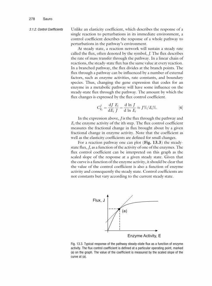
For a reaction pathway one can plot (Fig. 13.3) the steady-state flux, J, as a function of the activity of one of the enzymes. Theflux control coefficient can be interpreted on this graph as thescaled slope of the response at a given steady state. Given thatthe curve is a function of the enzyme activity, it should be clear thatthe value of the control coefficient is also a function of enzymeactivity and consequently the steady state. Control coefficients arenot constants but vary according to the current steady state.

Fig. 13.3. Typical response of the pathway steady-state flux as a function of enzymeactivity. The flux control coefficient is defined at a particular operating point, marked(a) on the graph. The value of the coefficient is measured by the scaled slope of thecurve at (a).

278 Sauro

One can also define a similar coefficient, the concentrationcontrol coefficient, with respect to species concentrations, thus:

CSEi¼ dS

dEi

Ei

S¼ d ln S

d ln Ei� S%=Ei%: ½5�

3.1.3. Relationship

Between Elasticities and

Control Coefficients

One of the most significant discoveries made early on in the devel-opment of BCT (Biochemical Control Theory) was the existence of arelationship between the elasticities and the control coefficients. Thisenabled one, for the first time, to describe in a general way, howproperties of individual enzymes could contribute to pathway beha-vior. More importantly, this relationship could be studied withoutthe need to solve, analytically, the system Eq. [1]. Particular exam-ples of these relationships will be given in the subsequent sections;here we will concentrate on the general relationship.

There are two related ways to derive the relationship betweenelasticities and control coefficients, the first is via the differentia-tion of the system Eq. [1] at steady state and the second by theconnectivity theorem.

System Equation Derivation. The system equation can bewritten more explicitly to show its dependence on the enzymeactivities (or any parameter set) of the system: Nv(s(E),E) = 0.By differentiating this expression with respect to E, we obtain

ds

dE¼ � N R

@v

@sL

� ��1

N R@v

@E: ½6�

The terms @v/@s and @v/@E are unscaled elasticities [See (69,37, 43, 53) for details of the derivation]. By scaling the equationwith the species concentration and enzyme activity, the left-handside becomes the concentration control coefficient expressed interms of scaled elasticities. The flux control coefficients can also bederived by differentiating the expression: J = v [s(p), p] to yield:

dJ

dE¼ I � @v

@sN R

@v

@sL

� ��1

N R

" #@v

@E: ½7�

Again, the flux expression can be scaled by E and J to yield thescaled flux control coefficients. These expressions, thoughunwieldy to some degree, are very useful for deriving symbolicexpressions relating the control coefficients to the elasticities. Avery thorough treatment together with the derivations of theseequations and much more can be found in Hofmeyr 2001.

Theorems. Examination of expressions [6] and [7] yields someadditional and unexpected relationships between the control coeffi-cients and the elasticities, called the summation and connectivitytheorems. These theorems were originally discovered by modelingsmall networks using an analog computer (Jim Burns, personalcommunication), but have since been derived by other means.


The flux summation theorem states that the sum of all the fluxcontrol coefficients in any pathway is equal to unity.

Xn

i¼1

CJi ¼ 1

It is also possible to derive a similar relationship with respect tospecies concentrations, namely

Xn

i¼1

CSk

i ¼ 0

In both relationships, n, is the number of reaction steps in thepathway. The flux summation theorem indicates that there is afinite amount of ‘‘control’’(or sensitivity) in a pathway and impliesthat control is shared between all steps. In addition, it states that ifone step were to gain control, then one or more other steps mustlose control.

Arguably, the most important relationship is between thecontrol coefficients and the elasticities.X

CJi e

iS ¼ 0

This theorem, and its relatives (88, 19, 20), is called the con-nectivity theorem and is probably the most significant relation-ship in computational systems biology because it relates twodifferent levels of description, the local level, in the form of elasti-cities, and the system level, in the form of control coefficients.Given the summation and connectivity theorems, it is possible tocombine them and solve for the control coefficients in terms of theelasticities. For small networks this approach is a viable way toderive the relationships (19), especially when combined with soft-ware such as MetaCon (81), which can compute the relationshipsalgebraically. Box 2 illustrates a simple example of this method.

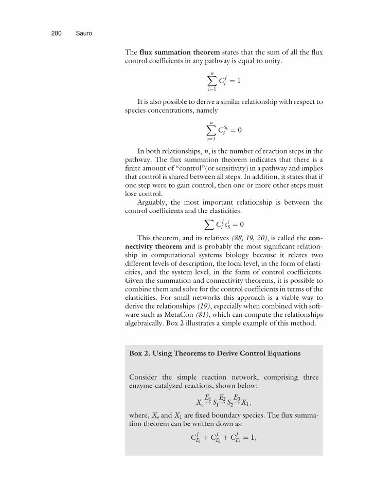
Box 2. Using Theorems to Derive Control Equations

Consider the simple reaction network, comprising threeenzyme-catalyzed reactions, shown below:

XE1

o! SE2

1! SE3

2!X1;

where, Xo and X1 are fixed boundary species. The flux summa-tion theorem can be written down as:

CJE1þ CJ

E2þ CJ

E3¼ 1;

280 Sauro

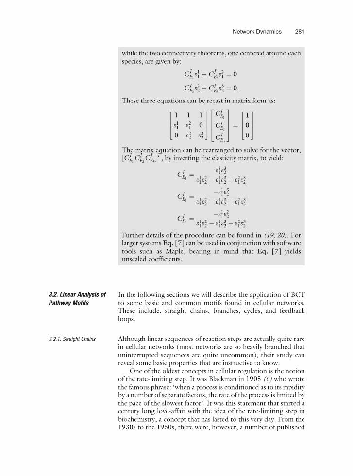
while the two connectivity theorems, one centered around eachspecies, are given by:

CJE1e11 þ CJ

E2e21 ¼ 0

CJE2e22 þ CJ

E3e32 ¼ 0:

These three equations can be recast in matrix form as:

1 1 1

e11 e2

1 0

0 e22 e3

2

264

375

CJE1

CJE2

CJE3

2664

3775 ¼

1

0

0

264375

The matrix equation can be rearranged to solve for the vector,½CJ

E1CJ

E2CJ

E3�T , by inverting the elasticity matrix, to yield:

CJE1¼ e2

1e32

e11e

22 � e1

1e32 þ e2

1e32

CJE2¼ �e1

1e32

e11e

22 � e1

1e32 þ e2

1e32

CJE3¼ �e1

1e22

e11e

22 � e1

1e32 þ e2

1e32

Further details of the procedure can be found in (19, 20). Forlarger systems Eq. [7] can be used in conjunction with softwaretools such as Maple, bearing in mind that Eq. [7] yieldsunscaled coefficients.

3.2. Linear Analysis of

Pathway MotifsIn the following sections we will describe the application of BCTto some basic and common motifs found in cellular networks.These include, straight chains, branches, cycles, and feedbackloops.

3.2.1. Straight Chains Although linear sequences of reaction steps are actually quite rarein cellular networks (most networks are so heavily branched thatuninterrupted sequences are quite uncommon), their study canreveal some basic properties that are instructive to know.

One of the oldest concepts in cellular regulation is the notionof the rate-limiting step. It was Blackman in 1905 (6) who wrotethe famous phrase: ‘when a process is conditioned as to its rapidityby a number of separate factors, the rate of the process is limited bythe pace of the slowest factor’. It was this statement that started acentury long love-affair with the idea of the rate-limiting step inbiochemistry, a concept that has lasted to this very day. From the1930s to the 1950s, there were, however, a number of published


papers which were highly critical of the concept, most notablyBurton (11), Morales (62) and Hearon (33) in particular. Unfor-tunately, much of this work did not find its way into the rapidlyexpanding fields of biochemistry and molecular biology after thesecond world war, and instead the intuitive idea first pronouncedby Blackman still remains today one of the basic but erroneousconcepts in cellular regulation. This is more surprising because asimple quantitative analysis shows that it cannot be true, and thereis ample experimental evidence (34, 10) to support the alternativenotion, that of shared control.

The confusion over the existence of rate-limiting steps stemsfrom a failure to realize that rates in cellular networks are governedby the law of mass-action, that is, if a concentration changes, thenso does its rate of reaction. Many researchers try to draw analogiesbetween cellular pathways and human experiences such as trafficcongestion on freeways or customer lines at shopping store check-outs. In each of these analogies, the rate of traffic and the rate ofcustomer checkouts does not depend on how many cars are in thetraffic line or how many customers are waiting. Such situationswarrant the correct use of the phrase rate-limiting step. Trafficcongestion and the customer line are rate-limiting because theonly way to increase the flow is to either widen the road or increasethe number of cash tills, that is, there is a single factor whichdetermines the rate of flow. In reaction networks, flow is governedby many factors, including the capacity of the reaction (Vmax) andsubstrate/ product/effector concentrations. In biological path-ways, rate-limiting steps are therefore the exception rather thanthe rule. Many hundreds of measurements of control coefficientshave born out this prediction. A simple quantitative study will alsomake this clear.

Consider a simple linear sequence of reactions governed byreversible mass-action rate laws:

Xo Ð S1 Ð S2 . . . Sn Ð Sn�1 ! Xn;

where Xo and Xn are fixed boundary species so that the pathwaycan sustain a steady state. If we assume the reaction rates to havethe simple form:

vj ¼ kj Sj �Sjþ1

qj

� �;

where qj is the thermodynamic equilibrium constant and kj theforward rate constant, we can compute the steady state flux, J, tobe (37):

J ¼Xo

Qnj¼1 qj �X1

Snl¼11=kl

Qnj¼l qj

:

282 Sauro

By modifying the rate laws to include an enzyme factor, such as:vj ¼ Ej kj Sj � Sjþ1

qj

� , we can also compute the flux control coeffi-

cients as (37):

CJi ¼

1=ki

Qnj¼i qj

Snl¼11=kl

Qnj¼l qj

:

Both equations show that the ability of a particular stepto limit the flux is governed not only by the particular stepitself but also by all other steps. Prior to the 1960s, this was awell-known result (62, 33), but was subsequently forgottenwith the rapid expansion of biochemistry and molecular biol-ogy. The control coefficient equation also puts limits on thevalues for the control coefficients in a linear chain, namely0 � CJ

i � 1 and

Xn

i¼1

CJi ¼ 1;

which is the flux control coefficient summation theorem. In alinear pathway the control of flux is therefore most likely to bedistributed among all steps in the pathway. This simple studyshows that the notion of the rate-limiting step is too simplisticand a better way to describe a reaction’s ability to limit flux is tostate its flux control coefficient.

Although a linear chain puts bounds on the values of the fluxcontrol coefficients, branched systems offer no such limits. It ispossible that increases in enzyme activity in one limb can decreasethe flux through another, hence the flux control coefficient can benegative. In addition, it is possible for the flux control coefficientto be greater than unity (Note 3).

3.2.2. Branched Systems Branching structures in metabolism are probably one of the mostcommon metabolic patterns. Even a pathway such as glycolysis,often depicted as a straight chain in textbooks, is in fact a highlybranched pathway.

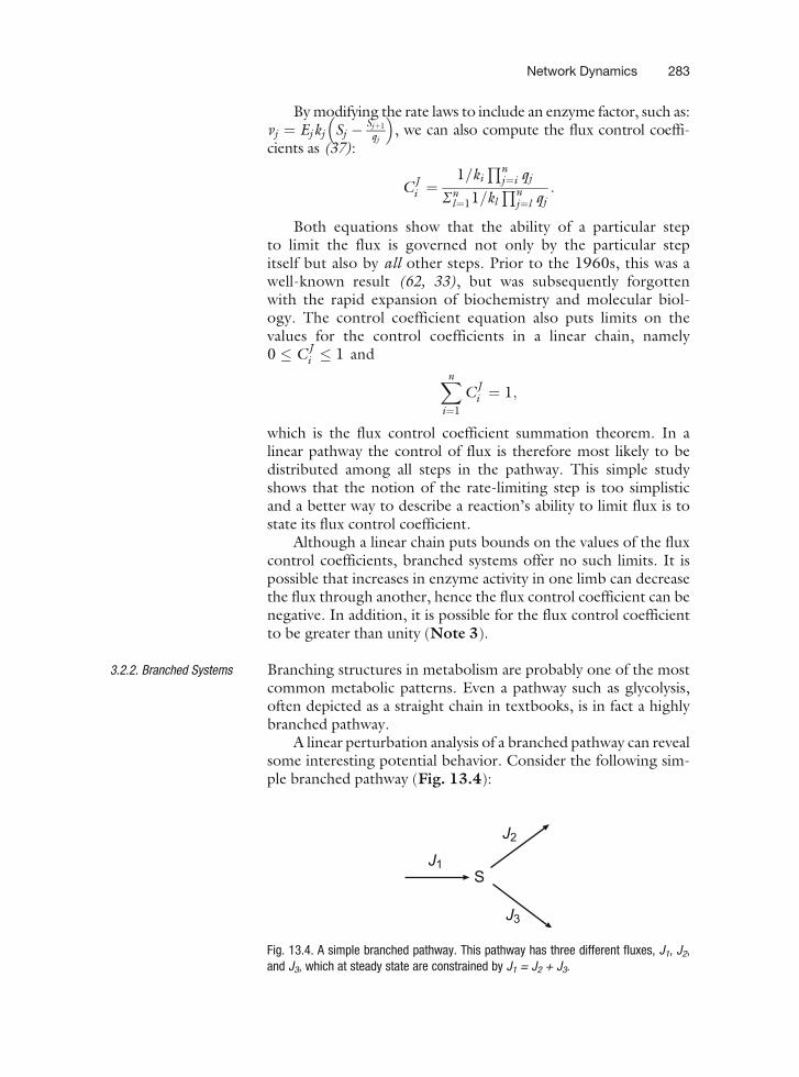
A linear perturbation analysis of a branched pathway can revealsome interesting potential behavior. Consider the following sim-ple branched pathway (Fig. 13.4):

Fig. 13.4. A simple branched pathway. This pathway has three different fluxes, J1, J2,and J3, which at steady state are constrained by J1 = J2 + J3.


where Ji are the steady state fluxes. By the law of conservation ofmass, at steady state, the fluxes in each limb are governed by therelationship:

J1 � ðJ2 þ J3Þ ¼ 0:

In terms of control theory, there will be four sets of controlcoefficients, one concerned with changes in the intermediate, S,and three sets corresponding to each of the individual fluxes.

Let the fraction of flux through J2 be given by a = J2/J1 and thefraction of flux through J3 be 1 � a = J3/J1. The flux controlcoefficients for step two and three can be derived and shown tobe equal to (19):

CJ2

E2¼ e1 � e3ð1� aÞ

e1 � e2a� e3ð1� aÞ40 CJ2

E3¼ e2ð1� aÞ

e1 � e2a� e3ð1� aÞ50:

Note that the flux control coefficient CJ2

E3is negative, indicating

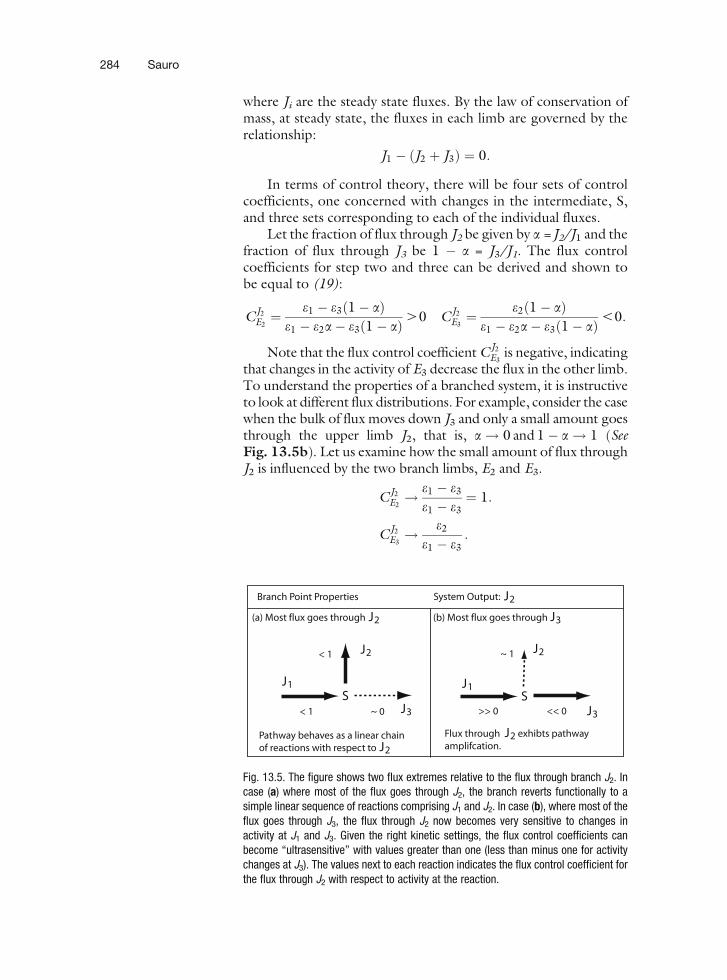
that changes in the activity of E3 decrease the flux in the other limb.To understand the properties of a branched system, it is instructiveto look at different flux distributions. For example, consider the casewhen the bulk of flux moves down J3 and only a small amount goesthrough the upper limb J2, that is, a! 0 and 1� a! 1 (SeeFig. 13.5b). Let us examine how the small amount of flux throughJ2 is influenced by the two branch limbs, E2 and E3.

CJ2

E2! e1 � e3

e1 � e3¼ 1:

CJ2

E3! e2

e1 � e3:

Branch Point Properties System Output:

S~ 0< 1

< 1

(a) Most flux goes through

Pathway behaves as a linear chain of reactions with respect to

J2

J2

S

J2

>> 0 << 0

~ 1

(b) Most flux goes through

Flux through exhibts pathwayamplifcation.

J3

J3

J2

J2

J2

J1 J1

J3

Fig. 13.5. The figure shows two flux extremes relative to the flux through branch J2. Incase (a) where most of the flux goes through J2, the branch reverts functionally to asimple linear sequence of reactions comprising J1 and J2. In case (b), where most of theflux goes through J3, the flux through J2 now becomes very sensitive to changes inactivity at J1 and J3. Given the right kinetic settings, the flux control coefficients canbecome ‘‘ultrasensitive’’ with values greater than one (less than minus one for activitychanges at J3). The values next to each reaction indicates the flux control coefficient forthe flux through J2 with respect to activity at the reaction.

284 Sauro

The first thing to note is that E2 tends to have proportionalinfluence over its own flux. Since J2 carries only a very smallamount of flux, any changes in E2 will have little effect on S,hence the flux through E2 is almost entirely governed by theactivity of E2. Because of the flux summation theorem and thefact that CJ2

E2¼ 1, the remaining two coefficients must be equal

and opposite in value. Since CJ2

E3is negative, CJ2

E1must be positive.

Unlike a linear chain, the values for CJ2

E2and CJ2

E1are not bounded

between zero and one and depending on the values of the elasti-cities it is possible for the control coefficients to greatly exceed one(48, 55). It is conceivable to arrange the kinetic constants so thatevery step in the branch has a control coefficient of unity (one ofwhich must be–1). Using the old terminology, we would concludefrom this that every step in the pathway is the rate-limiting step.

Let us now consider the other extreme, when most of the fluxis through J2, that is a! 0 and 1� a! 0 (See Fig. 13.5a). Underthese conditions the control coefficients yield:

CJ2

E2! e1

e1 � e2

CJ2

E3! 0

In this situation the pathway has effectively become a simplelinear chain. The influence of E3 on J2 is negligible. Figure 13.5summarizes the changes in sensitivities at a branch point.

3.2.3. Cyclic Systems Cyclic systems are extremely common in biochemical networks;they can be found in metabolic, genetic, and particularly signalingpathways. The functional role of cycles is not however fully under-stood, although in some cases their operational function is begin-ning to become clear. We can use linear perturbation analysis touncover some of the main properties of cycles.

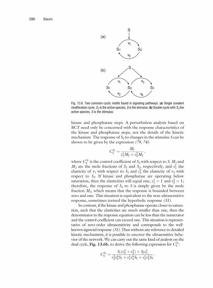
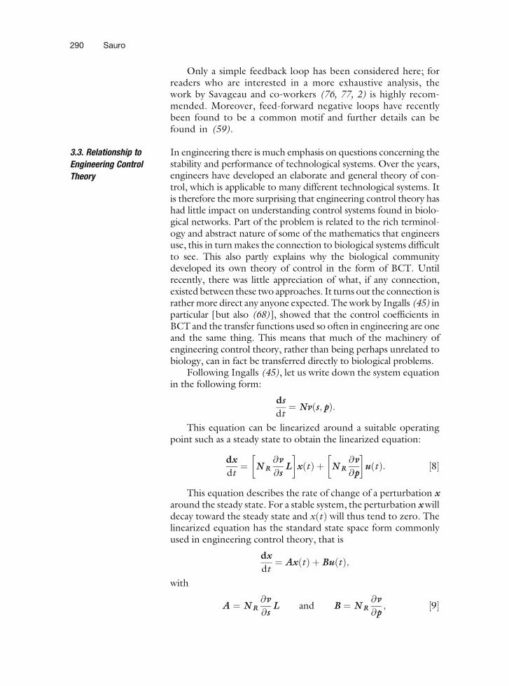
Figure 13.6 illustrates two common cyclic structures found insignaling pathways. Such cycles are often formed by a combinationof a kinase and a phosphatase. In many cases only one of themolecular species is active. For example, in Fig. 13.6a, let us assumethat S2 is the active (output) species, while in Fig. 13.6b, S3 is theactive (output) species. In a number of cases one observes multiplecycles formed by multi-site phosphorylation. Figure 13.6b shows acommon two-stage multi-site cycle. Note that in each case, the cyclesteady-state is maintained by the turnover of ATP. One questionthat can be addressed is how the steady-state output of each cycle, S2

and S3, depends on the input stimulus, S. This stimulus is assumedto be a stimulus of the kinase activity.

One approach to this is to build a detailed kinetic model andsolve for the steady-state concentration of S2 and S3 as a function ofS. This has been done analytically in a few cases (30, 31), butrequires the modeler to choose a particular kinetic model for the


kinase and phosphatase steps. A perturbation analysis based onBCT need only be concerned with the response characteristics ofthe kinase and phosphatase steps, not the details of the kineticmechanism. The response of S2 to changes in the stimulus S can beshown to be given by the expression (79, 74):

CS2

S ¼M1

e11M2 þ e2

2M1;

where CS2

S is the control coefficient of S2 with respect to S. M1 andM2 are the mole fractions of S1 and S2, respectively, and e1

1 theelasticity of v1 with respect to S1 and e2

2 the elasticity of v2 withrespect to S2. If kinase and phosphatase are operating belowsaturation, then the elasticities will equal one, e1

1 ¼ 1 and e22 ¼ 1;

therefore, the response of S2 to S is simply given by the molefraction M1, which means that the response is bounded betweenzero and one. This situation is equivalent to the non-ultrasensitiveresponse, sometimes termed the hyperbolic response (31).

In contrast, if the kinase and phosphatase operate closer to satura-tion, such that the elasticities are much smaller than one, then thedenominator in the response equation can be less than the numeratorand the control coefficient can exceed one. This situation is represen-tative of zero-order ultrasensitivity and corresponds to the well-known sigmoid response (31). Thus without any reference to detailedkinetic mechanisms, it is possible to uncover the ultrasensitive beha-vior of the network. We can carry out the same kind of analysis on thedual cycle, Fig. 13.6b, to derive the following expression for CS3

S :

CS3

S ¼S1ðe3

2 þ e22Þ þ S2e1

1

e32e

43S1 þ e1

1e43S2 þ e1

1e33S3

:

Fig. 13.6. Two common cyclic motifs found in signaling pathways. (a) Single covalentmodification cycle, S2 is the active species, S is the stimulus; (b) Double cycle with S3 theactive species, S is the stimulus.

286 Sauro

If we assume linear kinetics on each reaction such that all theelasticities equal one, the equation simplifies to

CS3

S ¼2S1 þ S2

S1 þ S2 þ S3:

This shows that given the right ratios for S1, S2, and S3, it ispossible for CS3

S4 1. Therefore, unlike the case of a single cycle

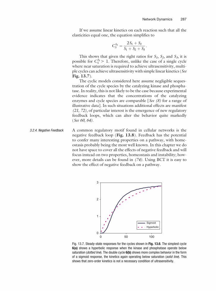
where near saturation is required to achieve ultrasensitivity, multi-ple cycles can achieve ultrasensitivity with simple linear kinetics (SeeFig. 13.7).

The cyclic models considered here assume negligible seques-tration of the cycle species by the catalyzing kinase and phospha-tase. In reality, this is not likely to be the case because experimentalevidence indicates that the concentrations of the catalyzingenzymes and cycle species are comparable [See (8) for a range ofillustrative data]. In such situations additional effects are manifest(21, 72), of particular interest is the emergence of new regulatoryfeedback loops, which can alter the behavior quite markedly(See 60, 64).

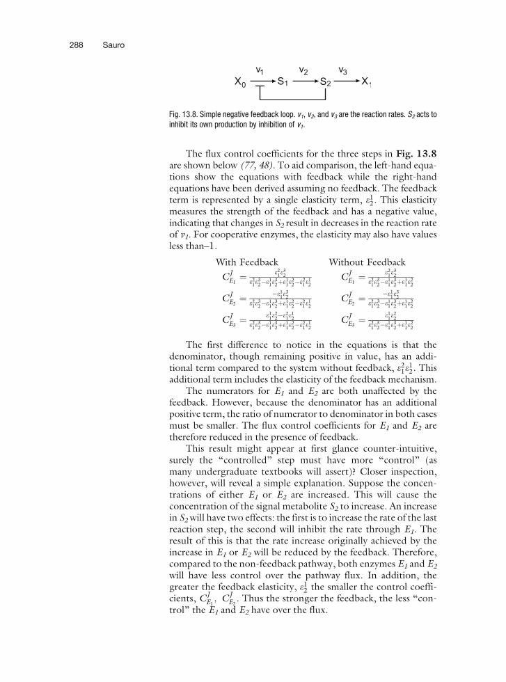
3.2.4. Negative Feedback A common regulatory motif found in cellular networks is thenegative feedback loop (Fig. 13.8). Feedback has the potentialto confer many interesting properties on a pathway, with home-ostasis probably being the most well known. In this chapter we donot have space to cover all the effects of negative feedback and willfocus instead on two properties, homeostasis and instability; how-ever, more details can be found in (74). Using BCT it is easy toshow the effect of negative feedback on a pathway.

Fig. 13.7. Steady-state responses for the cycles shown in Fig. 13.6. The simplest cycle6(a) shows a hyperbolic response when the kinase and phosphatase operate belowsaturation (dotted line). The double cycle 6(b) shows more complex behavior in the formof a sigmoid response, the kinetics again operating below saturation (solid line). Thisshows that zero-order kinetics is not a necessary condition of ultrasensitivity.


The flux control coefficients for the three steps in Fig. 13.8are shown below (77, 48). To aid comparison, the left-hand equa-tions show the equations with feedback while the right-handequations have been derived assuming no feedback. The feedbackterm is represented by a single elasticity term, e1

2. This elasticitymeasures the strength of the feedback and has a negative value,indicating that changes in S2 result in decreases in the reaction rateof v1. For cooperative enzymes, the elasticity may also have valuesless than–1.

With Feedback Without Feedback

CJE1¼ e2

1e32

e21e32�e1

1e32þe1

1e22�e2

1e12

CJE1¼ e2

1e32

e21e32�e1

1e32þe1

1e22

CJE2¼ �e1

1e32

e21e32�e1

1e32þe1

1e22�e2

1e12

CJE2¼ �e1

1e32

e21e32�e1

1e32þe1

1e22

CJE3¼ e1

1e22�e2

1e12

e21e32�e1

1e32þe1

1e22�e2

1e12

CJE3¼ e1

1e22

e21e32�e1

1e32þe1

1e22

The first difference to notice in the equations is that thedenominator, though remaining positive in value, has an addi-tional term compared to the system without feedback, e2

1e12. This

additional term includes the elasticity of the feedback mechanism.The numerators for E1 and E2 are both unaffected by the

feedback. However, because the denominator has an additionalpositive term, the ratio of numerator to denominator in both casesmust be smaller. The flux control coefficients for E1 and E2 aretherefore reduced in the presence of feedback.

This result might appear at first glance counter-intuitive,surely the ‘‘controlled’’ step must have more ‘‘control’’ (asmany undergraduate textbooks will assert)? Closer inspection,however, will reveal a simple explanation. Suppose the concen-trations of either E1 or E2 are increased. This will cause theconcentration of the signal metabolite S2 to increase. An increasein S2 will have two effects: the first is to increase the rate of the lastreaction step, the second will inhibit the rate through E1. Theresult of this is that the rate increase originally achieved by theincrease in E1 or E2 will be reduced by the feedback. Therefore,compared to the non-feedback pathway, both enzymes E1 and E2

will have less control over the pathway flux. In addition, thegreater the feedback elasticity, e1

2 the smaller the control coeffi-cients, CJ

E1; CJ

E2. Thus the stronger the feedback, the less ‘‘con-

trol’’ the E1 and E2 have over the flux.

Fig. 13.8. Simple negative feedback loop. v1, v2, and v3 are the reaction rates. S2 acts toinhibit its own production by inhibition of v1.

288 Sauro

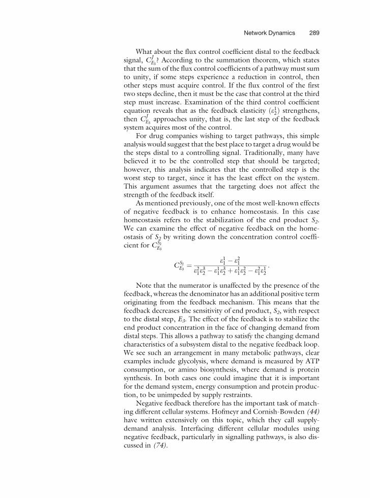
What about the flux control coefficient distal to the feedbacksignal, CJ

E3? According to the summation theorem, which states

that the sum of the flux control coefficients of a pathway must sumto unity, if some steps experience a reduction in control, thenother steps must acquire control. If the flux control of the firsttwo steps decline, then it must be the case that control at the thirdstep must increase. Examination of the third control coefficientequation reveals that as the feedback elasticity ðe1

2Þ strengthens,then CJ

E3approaches unity, that is, the last step of the feedback

system acquires most of the control.For drug companies wishing to target pathways, this simple

analysis would suggest that the best place to target a drug would bethe steps distal to a controlling signal. Traditionally, many havebelieved it to be the controlled step that should be targeted;however, this analysis indicates that the controlled step is theworst step to target, since it has the least effect on the system.This argument assumes that the targeting does not affect thestrength of the feedback itself.

As mentioned previously, one of the most well-known effectsof negative feedback is to enhance homeostasis. In this casehomeostasis refers to the stabilization of the end product S2.We can examine the effect of negative feedback on the home-ostasis of S2 by writing down the concentration control coeffi-cient for CS2

E3

CS2

E3¼ e1

1 � e21

e21e

32 � e1

1e32 þ e1

1e22 � e2

1e12

:

Note that the numerator is unaffected by the presence of thefeedback, whereas the denominator has an additional positive termoriginating from the feedback mechanism. This means that thefeedback decreases the sensitivity of end product, S2, with respectto the distal step, E3. The effect of the feedback is to stabilize theend product concentration in the face of changing demand fromdistal steps. This allows a pathway to satisfy the changing demandcharacteristics of a subsystem distal to the negative feedback loop.We see such an arrangement in many metabolic pathways, clearexamples include glycolysis, where demand is measured by ATPconsumption, or amino biosynthesis, where demand is proteinsynthesis. In both cases one could imagine that it is importantfor the demand system, energy consumption and protein produc-tion, to be unimpeded by supply restraints.

Negative feedback therefore has the important task of match-ing different cellular systems. Hofmeyr and Cornish-Bowden (44)have written extensively on this topic, which they call supply-demand analysis. Interfacing different cellular modules usingnegative feedback, particularly in signalling pathways, is also dis-cussed in (74).


Only a simple feedback loop has been considered here; forreaders who are interested in a more exhaustive analysis, thework by Savageau and co-workers (76, 77, 2) is highly recom-mended. Moreover, feed-forward negative loops have recentlybeen found to be a common motif and further details can befound in (59).

3.3. Relationship to

Engineering Control

Theory

In engineering there is much emphasis on questions concerning thestability and performance of technological systems. Over the years,engineers have developed an elaborate and general theory of con-trol, which is applicable to many different technological systems. Itis therefore the more surprising that engineering control theory hashad little impact on understanding control systems found in biolo-gical networks. Part of the problem is related to the rich terminol-ogy and abstract nature of some of the mathematics that engineersuse, this in turn makes the connection to biological systems difficultto see. This also partly explains why the biological communitydeveloped its own theory of control in the form of BCT. Untilrecently, there was little appreciation of what, if any connection,existed between these two approaches. It turns out the connection israther more direct any anyone expected. The work by Ingalls (45) inparticular [but also (68)], showed that the control coefficients inBCT and the transfer functions used so often in engineering are oneand the same thing. This means that much of the machinery ofengineering control theory, rather than being perhaps unrelated tobiology, can in fact be transferred directly to biological problems.

Following Ingalls (45), let us write down the system equationin the following form:

ds

dt¼ Nvðs; pÞ:

This equation can be linearized around a suitable operatingpoint such as a steady state to obtain the linearized equation:

dx

dt¼ N R

@v

@sL

� �xðtÞ þ N R

@v

@p

� �uðtÞ: ½8�

This equation describes the rate of change of a perturbation xaround the steady state. For a stable system, the perturbation x willdecay toward the steady state and xðtÞ will thus tend to zero. Thelinearized equation has the standard state space form commonlyused in engineering control theory, that is

dx

dt¼ AxðtÞ þ BuðtÞ;

with

A ¼ N R@v

@sL and B ¼ N R

@v

@p; ½9�

290 Sauro

u(t) is the input vector to the system, and may represent a set ofperturbations in boundary conditions, kinetic constants, ordepending on the particular model, gene expression changes.

Because of its equivalence to the state space form, Eq. [8]marks the entry point for describing biological control systemsusing the machinery of engineering control theory. In the follow-ing sections two applications, frequency analysis and stability ana-lysis, will be presented, which apply engineering control theory,rephrased using BCT, to biological problems.

3.3.1. Frequency Response It has been noted previously (3) that chemical networks can act assignal filters, that is, amplify or attenuate specific varying inputs. Itmay be the case that the ability to filter out specific frequencies hasbiological significance; for example, a cell may receive many dif-ferent varying inputs that enter a common signaling pathway;signals that have different frequencies could be identified. In addi-tion, multiple signals could be embedded in a single chemicalspecies (such as Ca2+) and demultiplexed by different target sys-tems. Finally, gene networks tend to be sources of noisy signalsthat may interfere with normal functioning; one could imaginespecific control systems that reduce the noise using high frequencyfiltering (15).

In steady state, sinusoidal inputs to a linear or linearizedsystem generate sinusoidal responses of the same frequency butof differing amplitude and phase. These differences are a functionsof frequency. For a more detailed explanation, Ingalls (45) pro-vides a readable introduction to concept of the frequency responseof a system in a biological context.

Whereas the linearized Eq. [8] describes the evolution of thesystem in the time domain, the frequency response must bedetermined in the frequency domain. Mathematically there is astandard approach, called the Laplace transform, to moving atime domain representation into the frequency representation.By taking the ratio of the Laplace transform of the output to thetransform of the input, one can derive the transfer function,which is a complex expression describing the relationshipbetween the input and the output in the frequency domain.The change in the amplitude between the input and output iscalculated by taking the absolute magnitude of the transfer func-tion. The phase shift that indicates how much the output signalhas been delayed can be computed by computing the phase angle.Note that under a linear treatment, the frequency does notchange.

In biological systems the outputs are often the species con-centrations or fluxes while the inputs are parameters such as kineticconstants, boundary conditions, or gene expression levels. By


taking the Laplace transform of Eq. [8] one can generate itstransfer function (45, 68) The transfer function for the speciesvector s with respect to a set of parameters p is given by:

RspðwÞ ¼ iwI �N R

@v

@sL

� ��1

N R@v

@p: ½10�

The response at zero frequency is given by

Rspð0Þ ¼ � N R

@v

@sL

� ��1

N R@v

@p:

Comparison of the above equation with the concentrationcontrol coefficient Equation [6] shows they are equivalent. Thisis the most important result because it links classical control theorydirectly with BCT. Moreover, it gives a biological interpretation tothe transfer functions so familiar to engineers. The transfer func-tions can be interpreted as a sensitivity of the amplitude and phaseof a signal to perturbations in the input signal. The control coeffi-cients of BCT are the transfer functions computed at zero fre-quency. Moreover, the denominator term in the transfer functionscan be used to ascertain the stability of the system, a topic that willbe covered in a later section.

Frequency Analysis of Simple Linear Reaction Chains. Thesimplest example to consider for a frequency analysis is a two-steppathway, that can be represented as a single gene expressing aprotein that undergoes degradation (Fig. 13.9). This simple sys-tem has been considered previously by Arkin (3) who used a con-ventional approach to compute the response. Here we will use theBCT approach, which allows us to express the frequency response interms of elasticities. Using Eq. [10] and assuming that the proteinconcentration has no effect on its synthesis, we can derive thefollowing expression:

CPG ¼

1

eDp þ iw

;

where eDP is the elasticity for protein degradation with respect to

the protein concentration. i is the complex number and w, thefrequency input. At zero frequency ðw ¼ 0Þ the equation reducesto the traditional control coefficient.

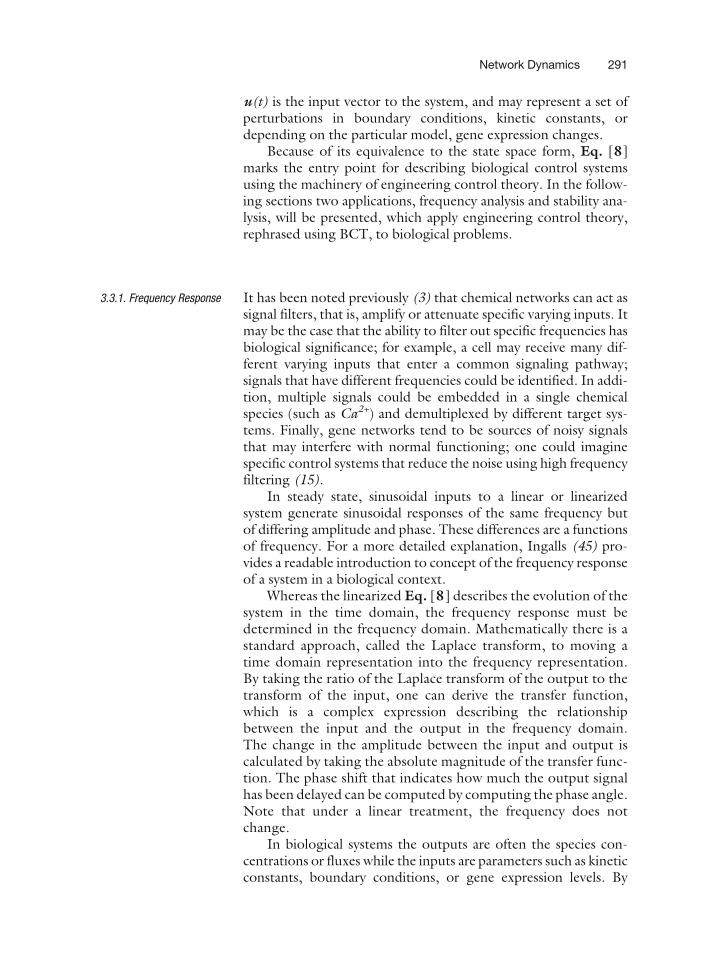
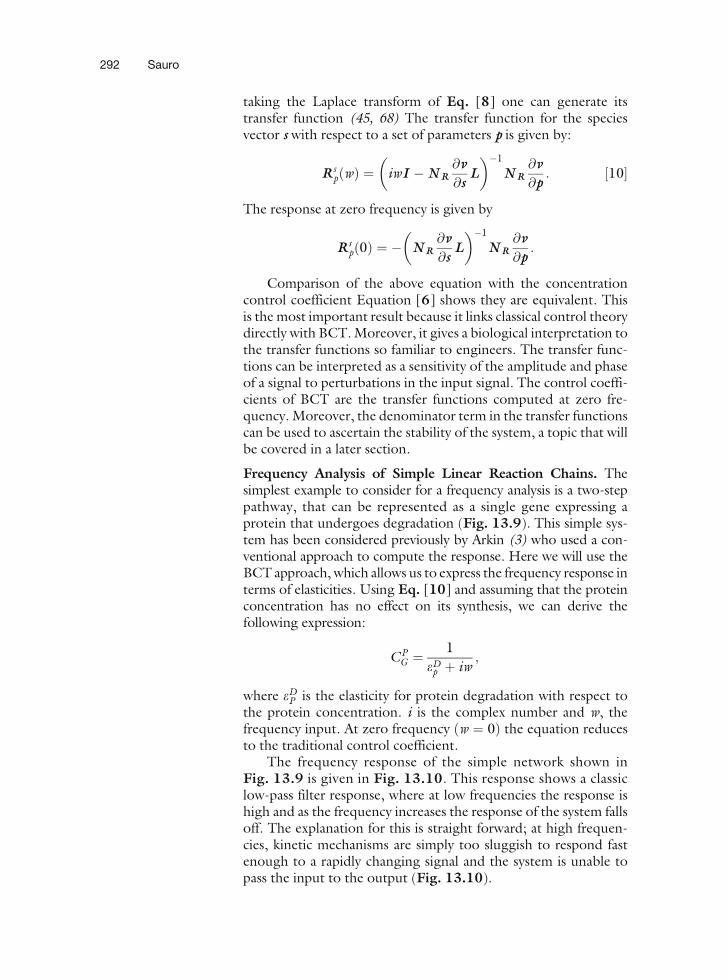
The frequency response of the simple network shown inFig. 13.9 is given in Fig. 13.10. This response shows a classiclow-pass filter response, where at low frequencies the response ishigh and as the frequency increases the response of the system fallsoff. The explanation for this is straight forward; at high frequen-cies, kinetic mechanisms are simply too sluggish to respond fastenough to a rapidly changing signal and the system is unable topass the input to the output (Fig. 13.10).

292 Sauro

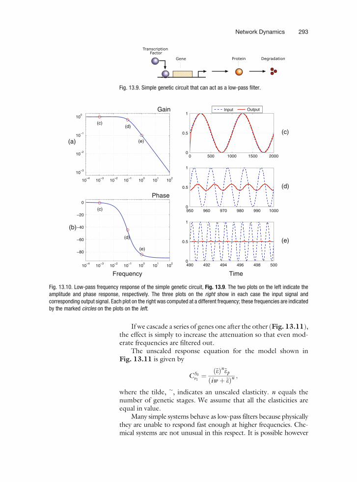
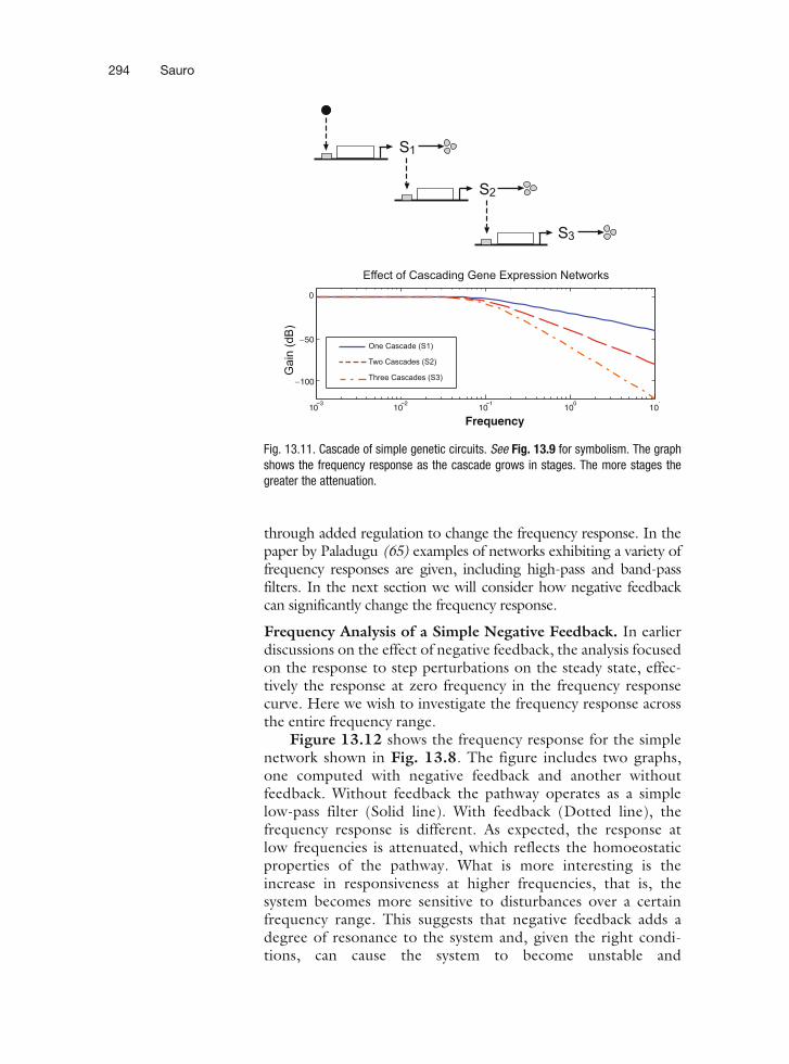
If we cascade a series of genes one after the other (Fig. 13.11),the effect is simply to increase the attenuation so that even mod-erate frequencies are filtered out.

The unscaled response equation for the model shown inFig. 13.11 is given by

CS3v1¼ ð~eÞn~ep

ðiw þ ~eÞn ;

where the tilde, �, indicates an unscaled elasticity. n equals thenumber of genetic stages. We assume that all the elasticities areequal in value.

Many simple systems behave as low-pass filters because physicallythey are unable to respond fast enough at higher frequencies. Che-mical systems are not unusual in this respect. It is possible however

10−4

10−3

10−2

10−1

100

101

102

10−3

10−2

10−1

100

(a)

10−4

10−3

10−2

10−1

100

101

102

−80

−60

−40

−20

0

(b)

0 500 1000 1500 20000

0.5

1

(c)

950 960 970 980 990 10000

0.5

1

(d)

490 492 494 496 498 5000

0.5

1

(e)

Gain

Phase

emiTycneuqerF

Input Output

(c)

(c)

(d)

(e)

(d)

(e)

Fig. 13.10. Low-pass frequency response of the simple genetic circuit, Fig. 13.9. The two plots on the left indicate theamplitude and phase response, respectively. The three plots on the right show in each case the input signal andcorresponding output signal. Each plot on the right was computed at a different frequency; these frequencies are indicatedby the marked circles on the plots on the left.

Fig. 13.9. Simple genetic circuit that can act as a low-pass filter.


through added regulation to change the frequency response. In thepaper by Paladugu (65) examples of networks exhibiting a variety offrequency responses are given, including high-pass and band-passfilters. In the next section we will consider how negative feedbackcan significantly change the frequency response.

Frequency Analysis of a Simple Negative Feedback. In earlierdiscussions on the effect of negative feedback, the analysis focusedon the response to step perturbations on the steady state, effec-tively the response at zero frequency in the frequency responsecurve. Here we wish to investigate the frequency response acrossthe entire frequency range.

Figure 13.12 shows the frequency response for the simplenetwork shown in Fig. 13.8. The figure includes two graphs,one computed with negative feedback and another withoutfeedback. Without feedback the pathway operates as a simplelow-pass filter (Solid line). With feedback (Dotted line), thefrequency response is different. As expected, the response atlow frequencies is attenuated, which reflects the homoeostaticproperties of the pathway. What is more interesting is theincrease in responsiveness at higher frequencies, that is, thesystem becomes more sensitive to disturbances over a certainfrequency range. This suggests that negative feedback adds adegree of resonance to the system and, given the right condi-tions, can cause the system to become unstable and

Fig. 13.11. Cascade of simple genetic circuits. See Fig. 13.9 for symbolism. The graphshows the frequency response as the cascade grows in stages. The more stages thegreater the attenuation.

294 Sauro

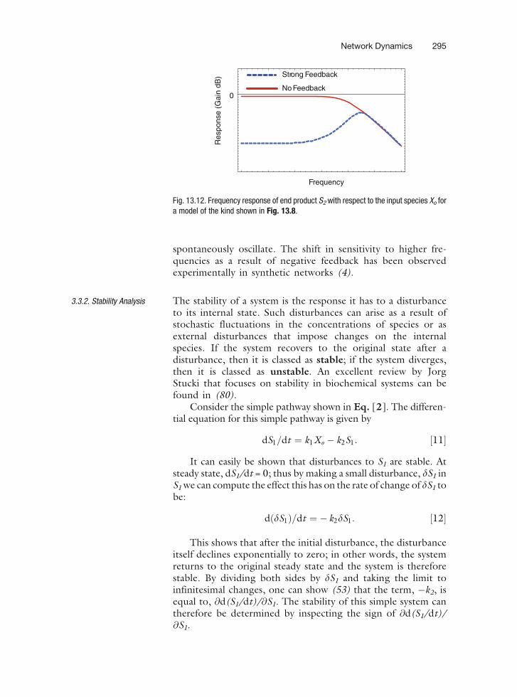
spontaneously oscillate. The shift in sensitivity to higher fre-quencies as a result of negative feedback has been observedexperimentally in synthetic networks (4).

3.3.2. Stability Analysis The stability of a system is the response it has to a disturbanceto its internal state. Such disturbances can arise as a result ofstochastic fluctuations in the concentrations of species or asexternal disturbances that impose changes on the internalspecies. If the system recovers to the original state after adisturbance, then it is classed as stable; if the system diverges,then it is classed as unstable. An excellent review by JorgStucki that focuses on stability in biochemical systems can befound in (80).

Consider the simple pathway shown in Eq. [2]. The differen-tial equation for this simple pathway is given by

dS1=dt ¼ k1Xo � k2S1: ½11�

It can easily be shown that disturbances to S1 are stable. Atsteady state, dS1/dt = 0; thus by making a small disturbance, dS1 inS1 we can compute the effect this has on the rate of change of dS1 tobe:

dðdS1Þ=dt ¼ � k2dS1: ½12�

This shows that after the initial disturbance, the disturbanceitself declines exponentially to zero; in other words, the systemreturns to the original steady state and the system is thereforestable. By dividing both sides by dS1 and taking the limit toinfinitesimal changes, one can show (53) that the term, �k2, isequal to, @d(S1/dt)/@S1. The stability of this simple system cantherefore be determined by inspecting the sign of @d(S1/dt)/@S1.

Frequency

Res

pons

e (G

ain

dB)

No Feedback

Strong Feedback

0

Fig. 13.12. Frequency response of end product S2 with respect to the input species Xo fora model of the kind shown in Fig. 13.8.


Now consider a change to the kinetic law, k1Xo, governing thefirst reaction. Instead of simple linear kinetics let us use a coopera-tive enzyme which is activated by the product S1. The rate law forthe first reaction is now given by:

v1 ¼k1XoðXo þ 1ÞðS1 þ 1Þ2

ðS1 þ 1Þ2ðXo þ 1Þ2 þ 80000:

Setting Xo = 1, k1 = 100, k2 = 0.14, a steady-state concentra-tion of S1 can be determined to be 66.9. Evaluating the derivative@d(S1/dt)/@S1 at this steady state yields a value of 0.084, which isclearly a positive value. This means that any disturbance to S1 at thisparticular steady state will cause S1 to increase; in other words, thissteady state is unstable.

For single variable systems the question of stability reduces todetermining the sign of the @d(S1/dt)/@S1 derivative. For largersystems the stability of a system can be determined by looking at allthe terms @d(Si/dt)/@Si which are given collectively by theexpression:

dðds=dtÞds

¼ J ; ½13�

where J is called the Jacobian matrix containing elements of theform @d(Si/dt)/@Si. Equation [12] can be generalized to:

dðdsÞdt¼ J ds:

Analysis shows that solutions to the disturbance equations[12] and [13] are sums of exponentials where the exponents ofthe exponentials are given by the eigenvalues of the Jacobianmatrix, J (53). If the eigenvalues are negative then the exponentsdecay (stable), whereas if they are positive then the exponentsgrow (unstable).

Another way to obtain the eigenvalues is to look at the roots(often called the poles in engineering) of the characteristic equa-tion, which can be found in the denominator of the transferfunction, Eq. [10]. For stability, the real parts of all the polesof the transfer function should be negative. If any pole is positive,then the system is unstable. The characteristic equation can bewritten as a polynomial, where the order of the polynomialreflects the size of the model.

ansn þ an�1sn�1 þ . . .þ a1s þ ao ¼ 0

A test for stability is that all the coefficients of the poly-nomial must have the same sign if all the poles are to havenegative real parts. Also it is necessary for all the coefficients

296 Sauro

to be nonzero for stability. A technique called the Routh-Hurwitzcriterion can be used to determine the stability. This proce-dure involves the construction of a ‘‘Routh Array’’ shown inTable 13.2. The third and fourth rows of the table are computedusing the relations:

b1 ¼an�1an�2 � anan�3

an�1b2 ¼

an�1an�4 � anan�5

an�1etc:

c1 ¼b1an�3 � b2an�1

b1c2 ¼

b1an�5 � b3an�1

b1etc:

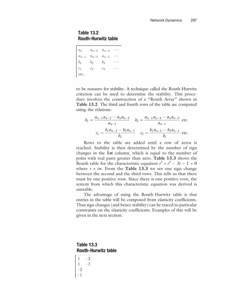
Rows to the table are added until a row of zeros isreached. Stability is then determined by the number of signchanges in the 1st column, which is equal to the number ofpoles with real parts greater than zero. Table 13.3 shows theRouth table for the characteristic equation s3 + s2 � 3s � 1 = 0where s = iw. From the Table 13.3 we see one sign changebetween the second and the third rows. This tells us that theremust be one positive root. Since there is one positive root, thesystem from which this characteristic equation was derived isunstable.

The advantage of using the Routh-Hurwitz table is thatentries in the table will be composed from elasticity coefficients.Thus sign changes (and hence stability) can be traced to particularconstraints on the elasticity coefficients. Examples of this will begiven in the next section.

Table 13.2Routh-Hurwitz table

an an−2 an−4 · · ·an−1 an−3 an−5 · · ·b1 b2 b3 · · ·c1 c2 c3 · · ·etc.

1 –31 –1–2–1

Table 13.3Routh-Hurwitz table


3.4. Dynamic Motifs

3.4.1. Bistable Systems

The question of stability leads on to the study of systems with non-trivial behaviors. In the previous section a model was considered,which was shown to be unstable. This model was described by thefollowing set of rate equations:

v1 ¼k1XoðXo þ 1ÞðS1 þ 1Þ2

ðS1 þ 1Þ2ðXo þ 1Þ2 þ 80000;

v2 ¼ k2S1:

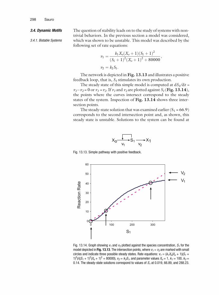
The network is depicted in Fig. 13.13 and illustrates a positivefeedback loop, that is, S1 stimulates its own production.

The steady state of this simple model is computed at dS1/dt =v1�v2 = 0 or v1 = v2. If v1 and v2 are plotted against S1 (Fig. 13.14),the points where the curves intersect correspond to the steadystates of the system. Inspection of Fig. 13.14 shows three inter-section points.

The steady-state solution that was examined earlier (S1 = 66.9)corresponds to the second intersection point and, as shown, thissteady state is unstable. Solutions to the system can be found at

Fig. 13.14. Graph showing v1 and v2 plotted against the species concentration, S1 for themodel depicted in Fig. 13.13. The intersection points, where v1 = v2 are marked with smallcircles and indicate three possible steady states. Rate equations: v1 = (k1Xo(Xo + 1)(S1 +1)2)/((S1 + 1)2(Xo + 1)2 + 80000), v2 = k2S1, and parameter values Xo = 1, k1 = 100, k2 =0.14. The steady-state solutions correspond to values of S1 at 0.019, 66.89, and 288.23.

Fig. 13.13. Simple pathway with positive feedback.

298 Sauro

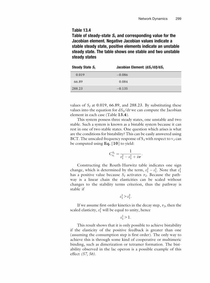
values of S1 at 0.019, 66.89, and 288.23. By substituting thesevalues into the equation for dS1/dt we can compute the Jacobianelement in each case (Table 13.4).

This system possess three steady states, one unstable and twostable. Such a system is known as a bistable system because it canrest in one of two stable states. One question which arises is whatare the conditions for bistability? This can be easily answered usingBCT. The unscaled frequency response of S1 with respect to v1 canbe computed using Eq. [10] to yield:

CS1v1¼ 1

e21 � e1

1 þ iw:

Constructing the Routh-Hurwitz table indicates one signchange, which is determined by the term, e2

1 � e11. Note that e1

1

has a positive value because S1 activates v1. Because the path-way is a linear chain the elasticities can be scaled withoutchanges to the stability terms criterion, thus the pathway isstable if

e114e2

1:

If we assume first-order kinetics in the decay step, v2, then thescaled elasticity, e2

1 will be equal to unity, hence

e1141:

This result shows that it is only possible to achieve bistabilityif the elasticity of the positive feedback is greater than one(assuming the consumption step is first order). The only way toachieve this is through some kind of cooperative or multimericbinding, such as dimerization or tetramer formation. The bist-ability observed in the lac operon is a possible example of thiseffect (57, 56).

Table 13.4Table of steady-state S1 and corresponding value for theJacobian element. Negative Jacobian values indicate astable steady state, positive elements indicate an unstablesteady state. The table shows one stable and two unstablesteady states

Steady State S1 Jacobian Element: (dS1/dt)/dS1

0.019 �0.086

66.89 0.084

288.23 �0.135


3.4.2. Feedback and

Oscillatory Systems

The study of oscillatory systems in biochemistry has a long historydating back to at least the 1950s. Until recently, however, therewas very little interest in the topic from mainstream molecularbiology. In fact, one suspects that the concept of oscillatory beha-vior in cellular networks was considered more a curiosity, and arare one at that, than anything serious. With the advent of newmeasurement technologies, particulary high-quality microscopy,and the ability to monitor specific protein levels using GFP andother fluorescence techniques, a whole new world has opened upto many experimentalists. Of particular note is the recent discoveryof oscillatory dynamics in the p53/Mdm2 couple (54, 26) and Nf-kB (41) signaling; thus rather than being a mere curiosity, oscilla-tory behavior is in fact an important, though largely unexplained,phenomenon in cells.

Basic Oscillatory Designs. There are two basic kinds of oscillatorydesigns, one based on negative feedback and a second based on acombination of negative and positive feedback. Both kinds of oscilla-tory design have been found in biological systems. An excellent reviewof these oscillators and specific biological examples can be found in (84,18). A more technical discussion can be found in (83, 82).

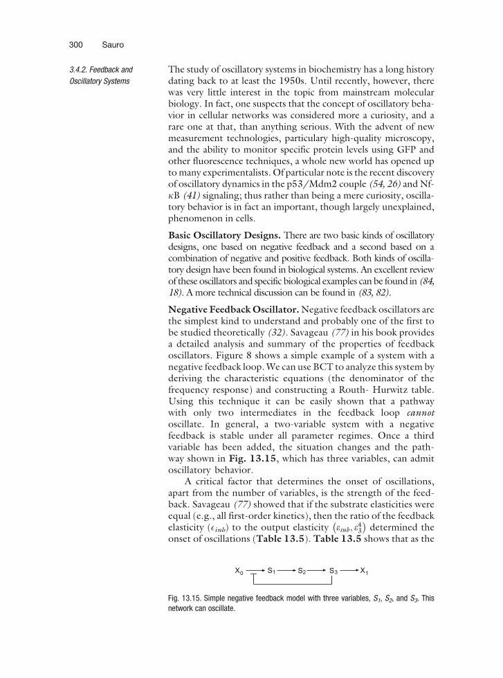
Negative Feedback Oscillator. Negative feedback oscillators arethe simplest kind to understand and probably one of the first tobe studied theoretically (32). Savageau (77) in his book providesa detailed analysis and summary of the properties of feedbackoscillators. Figure 8 shows a simple example of a system with anegative feedback loop. We can use BCT to analyze this system byderiving the characteristic equations (the denominator of thefrequency response) and constructing a Routh- Hurwitz table.Using this technique it can be easily shown that a pathwaywith only two intermediates in the feedback loop cannotoscillate. In general, a two-variable system with a negativefeedback is stable under all parameter regimes. Once a thirdvariable has been added, the situation changes and the path-way shown in Fig. 13.15, which has three variables, can admitoscillatory behavior.

A critical factor that determines the onset of oscillations,apart from the number of variables, is the strength of the feed-back. Savageau (77) showed that if the substrate elasticities wereequal (e.g., all first-order kinetics), then the ratio of the feedbackelasticity (Einh) to the output elasticity esub ; e4

3

� �determined the

onset of oscillations (Table 13.5). Table 13.5 shows that as the

Fig. 13.15. Simple negative feedback model with three variables, S1, S2, and S3. Thisnetwork can oscillate.

300 Sauro

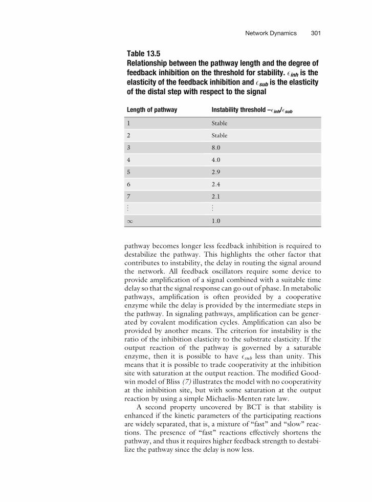
pathway becomes longer less feedback inhibition is required todestabilize the pathway. This highlights the other factor thatcontributes to instability, the delay in routing the signal aroundthe network. All feedback oscillators require some device toprovide amplification of a signal combined with a suitable timedelay so that the signal response can go out of phase. In metabolicpathways, amplification is often provided by a cooperativeenzyme while the delay is provided by the intermediate steps inthe pathway. In signaling pathways, amplification can be gener-ated by covalent modification cycles. Amplification can also beprovided by another means. The criterion for instability is theratio of the inhibition elasticity to the substrate elasticity. If theoutput reaction of the pathway is governed by a saturableenzyme, then it is possible to have Esub less than unity. Thismeans that it is possible to trade cooperativity at the inhibitionsite with saturation at the output reaction. The modified Good-win model of Bliss (7) illustrates the model with no cooperativityat the inhibition site, but with some saturation at the outputreaction by using a simple Michaelis-Menten rate law.

A second property uncovered by BCT is that stability isenhanced if the kinetic parameters of the participating reactionsare widely separated, that is, a mixture of ‘‘fast’’ and ‘‘slow’’ reac-tions. The presence of ‘‘fast’’ reactions effectively shortens thepathway, and thus it requires higher feedback strength to destabi-lize the pathway since the delay is now less.

Table 13.5Relationship between the pathway length and the degree offeedback inhibition on the threshold for stability. Einh is theelasticity of the feedback inhibition and Esub is the elasticityof the distal step with respect to the signal

Length of pathway Instability threshold –�inh/�sub

1 Stable

2 Stable

3 8.0

4 4.0

5 2.9

6 2.4

7 2.1

..

. ...

1 1.0


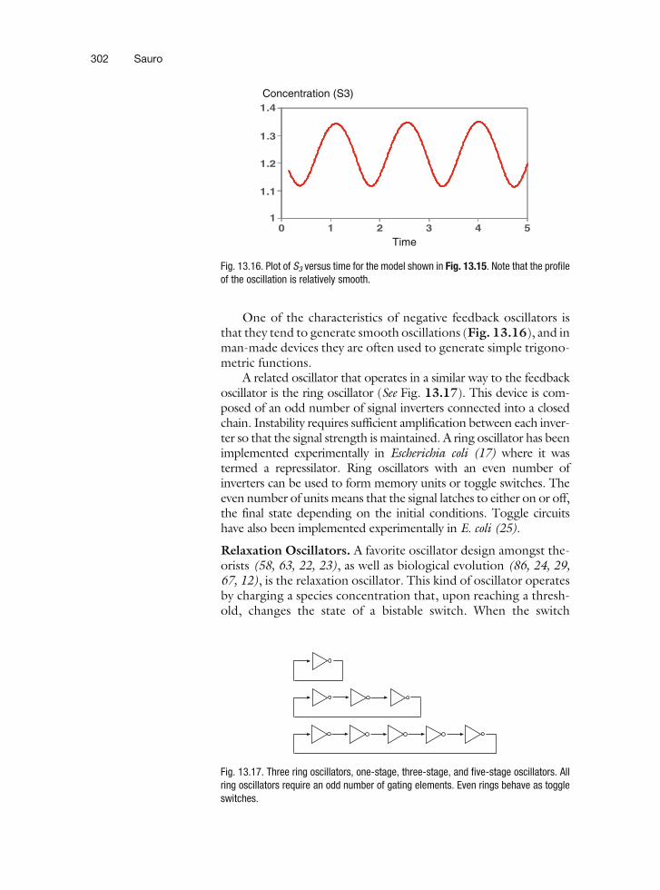
One of the characteristics of negative feedback oscillators isthat they tend to generate smooth oscillations (Fig. 13.16), and inman-made devices they are often used to generate simple trigono-metric functions.

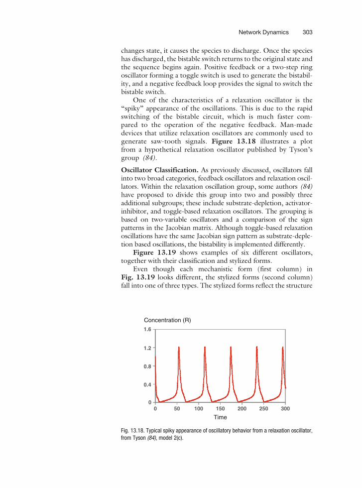
A related oscillator that operates in a similar way to the feedbackoscillator is the ring oscillator (See Fig. 13.17). This device is com-posed of an odd number of signal inverters connected into a closedchain. Instability requires sufficient amplification between each inver-ter so that the signal strength is maintained. A ring oscillator has beenimplemented experimentally in Escherichia coli (17) where it wastermed a repressilator. Ring oscillators with an even number ofinverters can be used to form memory units or toggle switches. Theeven number of units means that the signal latches to either on or off,the final state depending on the initial conditions. Toggle circuitshave also been implemented experimentally in E. coli (25).

Relaxation Oscillators. A favorite oscillator design amongst the-orists (58, 63, 22, 23), as well as biological evolution (86, 24, 29,67, 12), is the relaxation oscillator. This kind of oscillator operatesby charging a species concentration that, upon reaching a thresh-old, changes the state of a bistable switch. When the switch

Fig. 13.17. Three ring oscillators, one-stage, three-stage, and five-stage oscillators. Allring oscillators require an odd number of gating elements. Even rings behave as toggleswitches.

Concentration (S3)

Time

1

1.1

1.2

1.3

1.4

0 1 2 3 4 5

Fig. 13.16. Plot of S3 versus time for the model shown in Fig. 13.15. Note that the profileof the oscillation is relatively smooth.

302 Sauro

changes state, it causes the species to discharge. Once the specieshas discharged, the bistable switch returns to the original state andthe sequence begins again. Positive feedback or a two-step ringoscillator forming a toggle switch is used to generate the bistabil-ity, and a negative feedback loop provides the signal to switch thebistable switch.

One of the characteristics of a relaxation oscillator is the‘‘spiky’’ appearance of the oscillations. This is due to the rapidswitching of the bistable circuit, which is much faster com-pared to the operation of the negative feedback. Man-madedevices that utilize relaxation oscillators are commonly used togenerate saw-tooth signals. Figure 13.18 illustrates a plotfrom a hypothetical relaxation oscillator published by Tyson’sgroup (84).

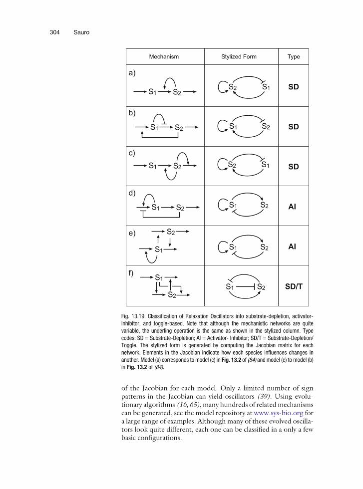
Oscillator Classification. As previously discussed, oscillators fallinto two broad categories, feedback oscillators and relaxation oscil-lators. Within the relaxation oscillation group, some authors (84)have proposed to divide this group into two and possibly threeadditional subgroups; these include substrate-depletion, activator-inhibitor, and toggle-based relaxation oscillators. The grouping isbased on two-variable oscillators and a comparison of the signpatterns in the Jacobian matrix. Although toggle-based relaxationoscillations have the same Jacobian sign pattern as substrate-deple-tion based oscillations, the bistability is implemented differently.

Figure 13.19 shows examples of six different oscillators,together with their classification and stylized forms.

Even though each mechanistic form (first column) inFig. 13.19 looks different, the stylized forms (second column)fall into one of three types. The stylized forms reflect the structure

0

0.4

0.8

1.2

1.6

0 50 100 150 200 250 300

Time

Concentration (R)

Fig. 13.18. Typical spiky appearance of oscillatory behavior from a relaxation oscillator,from Tyson (84), model 2(c).


of the Jacobian for each model. Only a limited number of signpatterns in the Jacobian can yield oscillators (39). Using evolu-tionary algorithms (16, 65), many hundreds of related mechanismscan be generated, see the model repository at www.sys-bio.org fora large range of examples. Although many of these evolved oscilla-tors look quite different, each one can be classified in a only a fewbasic configurations.

Fig. 13.19. Classification of Relaxation Oscillators into substrate-depletion, activator-inhibitor, and toggle-based. Note that although the mechanistic networks are quitevariable, the underling operation is the same as shown in the stylized column. Typecodes: SD = Substrate-Depletion; AI = Activator- Inhibitor; SD/T = Substrate-Depletion/Toggle. The stylized form is generated by computing the Jacobian matrix for eachnetwork. Elements in the Jacobian indicate how each species influences changes inanother. Model (a) corresponds to model (c) in Fig. 13.2 of (84) and model (e) to model (b)in Fig. 13.2 of (84).

304 Sauro

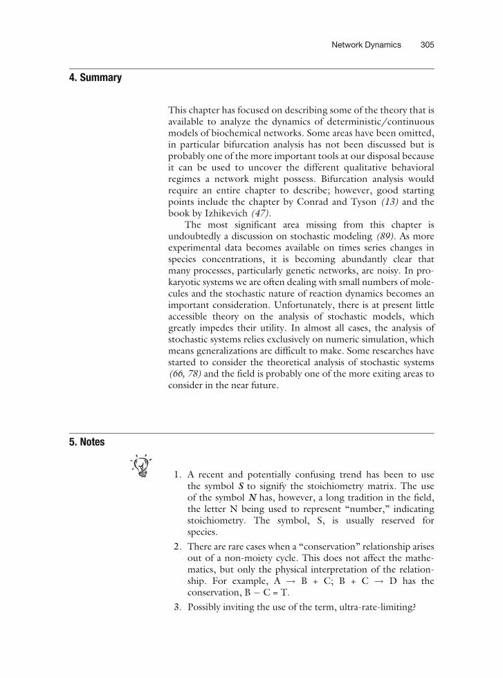
4. Summary

This chapter has focused on describing some of the theory that isavailable to analyze the dynamics of deterministic/continuousmodels of biochemical networks. Some areas have been omitted,in particular bifurcation analysis has not been discussed but isprobably one of the more important tools at our disposal becauseit can be used to uncover the different qualitative behavioralregimes a network might possess. Bifurcation analysis wouldrequire an entire chapter to describe; however, good startingpoints include the chapter by Conrad and Tyson (13) and thebook by Izhikevich (47).

The most significant area missing from this chapter isundoubtedly a discussion on stochastic modeling (89). As moreexperimental data becomes available on times series changes inspecies concentrations, it is becoming abundantly clear thatmany processes, particularly genetic networks, are noisy. In pro-karyotic systems we are often dealing with small numbers of mole-cules and the stochastic nature of reaction dynamics becomes animportant consideration. Unfortunately, there is at present littleaccessible theory on the analysis of stochastic models, whichgreatly impedes their utility. In almost all cases, the analysis ofstochastic systems relies exclusively on numeric simulation, whichmeans generalizations are difficult to make. Some researches havestarted to consider the theoretical analysis of stochastic systems(66, 78) and the field is probably one of the more exiting areas toconsider in the near future.

5. Notes

1. A recent and potentially confusing trend has been to usethe symbol S to signify the stoichiometry matrix. The useof the symbol N has, however, a long tradition in the field,the letter N being used to represent ‘‘number,’’ indicatingstoichiometry. The symbol, S, is usually reserved forspecies.

2. There are rare cases when a ‘‘conservation’’ relationship arisesout of a non-moiety cycle. This does not affect the mathe-matics, but only the physical interpretation of the relation-ship. For example, A ! B + C; B + C ! D has theconservation, B � C = T.

3. Possibly inviting the use of the term, ultra-rate-limiting?


6. Reading List

The following lists books and articles that cover the material in thischapter in much more depth.

Introductory and

Advanced Texts on

Systems Analysis

Fell, D (1996) Understanding the Control of Metabolism,Ashgate Publishing, ISBN: 185578047X

Heinrich R, Schuster S (1996) The Regulation of CellularSystems. Chapman and Hall, ISBN: 0412032619

Klipp E, et al. (2005) Systems Biology in Practice, Concepts,Implementation and Application. Wiley-VCH Verlag, ISBN:3527310789

Izhikevich, E. M. (2007) Dynamical Systems in Neuroscience:The Geometry of Excitability and Bursting, MIT Press, ISBN:0262090430

Control Theory Ingalls, B. P. (2004) A frequency domain approach to sensitivityanalysis of biochemical systems, Journal of Physical Chemistry B,108, 1143–1152

Bistablilty and

Oscillations

Tyson J, et al. (2003) Sniffers, buzzers, toggles and blinkers:dynamics of regulatory and signaling pathways in the cell. CurrentOpinion in Cell Biology, 15, 221–231

Stochastic Modeling Wilkinson D. J. (2006) Stochastic Modeling for Systems Biology.Chapman and Hall, ISBN: 1584885408

Acknowledgments

I wish to acknowledge Ravishankar R. Vallabhajosyula for assis-tance in preparing the simulation data and figures for the genecascade circuits. This work was support by a generous grant fromthe NSF (award number CCF- 0432190).

References

1. Altan-Bonnet G, Germain RN (2005).Modeling T cell antigen discriminationbased on feedback control of digital ERKresponses. PLoS Biol 3(11):1925–1938.

2. Alves R, Savageau MA (2000). Effect ofoverall feedback inhibition in unbranchedbiosynthetic pathways. Biophys J 79:2290–2304.

3. Arkin AP (2000). Signal Processing by Bio-chemical Reaction Networks. In J. Walleczek(Ed.), Self-Organized Biological Dynamicsand Nonlinear Control, pp. 112–114. Cam-bridge University Press.

4. Austin DW, Allen MS, McCollum JM, DarRD, Wilgus JR, Sayler GS, Samatova NF,et al. (2006). Gene network shaping of

306 Sauro

inherent noise spectra. Nature 439(7076):608–611.

5. Bakker BM, Westerhoff HV, Opperdoes FR,Michels PAM (2000). Metabolic controlanalysis of glycolysis in trypanosomes as anapproach to improve selectivity and effec-tiveness of drugs. Mol Biochem Parasitology106:1–10.

6. Blackman FF (1905). Optima and limitingfactors. Ann Botany 19:281–295.

7. Bliss RD, Painter PR, Marr AG (1982). Roleof feedback inhibition in stabilizing the clas-sical operon. J Theor Biol 97(2):177–193.

8. Bluthgen N, Bruggeman FJ, Legewie S,Herzel H, Westerhoff HV, KholodenkoBN (2006). Effects of sequestration on sig-nal transduction cascades. FEBS J 273(5):895–906.

9. Burns JA (1971). Studies on ComplexEnzyme Systems. Ph. D. thesis, Universityof Edinburgh. http://www.cds.caltech.edu/hsauro/Burns/jimBurns.pdf

10. Burrell MM, Mooney PJ, Blundy M,Carter D, Wilson F, Green J, Blundy KS,et al. (1994). Genetic manipulation of 6-phosphofructokinase in potato tubers. Planta194:95–101.

11. Burton AC (1936). The basis of the princi-ple of the master reaction in biology. J CellComp Physiol 9(1):1–14.

12. Chen KC, Calzone L, Csikasz-Nagy A,Cross FR, Novak B, Tyson JJ (2004).Integrative analysis of cell cycle controlin budding yeast. Mol Biol Cell 15(8):3841–3862.

13. Conrad ED, Tyson JJ (2006). ModelingMoelcular Interaction Networks with Non-linear Ordinary Differential Equations. InJ. S. Zoltan Szallasi and V. Periwal (Eds.),System Modeling in Cellular Biology FromConcepts to Nuts and Bolts, Chapter 6, pp.97–123. MIT Press.

14. Cornish-Bowden A, Hofmeyr JHS (2002).The Role of Stoichiometric Analysis in Stu-dies of Metabolism: An Example J TheorBiol 216:179–191.

15. Cox C, McCollum J, Austin D, Allen M,Dar R, Simpson M (2006). Frequencydomain analysis of noise in simple gene cir-cuits. Chaos 16(2):26102–26102.

16. Deckard A, Sauro HM (2004). Preliminarystudies on the in silico evolution of biochem-ical networks. Chembiochem 5:1423–31.

17. Elowitz MB, Leibler S (2000). A syntheticoscillatory network of transcriptional regu-lators. Nature 403:335–338.

18. Fall CP, Marland ES, Wagner JM, Tyson JJ(2002). Computational Cell Biology.Springer-Verlag.

19. Fell DA, Sauro HM (1985a). Metaboliccontrol analysis: additional relationshipsbetween elasticities and control coefficients.Eur J Biochem 148:555–561.

20. Fell DA, Sauro HM (1985b) Substratecycles: do they really cause amplification?Biochem Soc Trans 13:762–763.

21. Fell DA, Sauro HM (1990). Metaboliccontrol analysis: the effects of high en-zyme concentrations. Eur J Biochem 192:183–187.

22. Field RJ, Koros E, Noyes RM (1972). Oscil-lations in chemical systems, Part 2. Thor-ough analysis of temporal oscillations in thebromateceriummalonic acid system. J AmChem Soc 94:8649–8664.

23. Field RJ, Noyes RM (1974). Oscillations inchemical systems. IV. Limit cycle behaviorin a model of a real chemical reaction. JChem Phys 60(5):1877–1884.

24. FitzHugh R (1955). Mathematical modelsof threshold phenomena in the nerve mem-brane. Bull Math Biophys 17:257–278.

25. Gardner TS, Cantor CR, Collins JJ (2000).Construction of a genetic toggle switch inEscherichia coli. Nature 403:339–342.

26. Geva-Zatorsky N, Rosenfeld N, Itzkovitz S,Milo R, Sigal A, Dekel E, Yarnitzky T, et al.(2006). Oscillations and variability in thep53 system. Mol Syst Biol 2:2006–2006.

27. Gillespie DT (1976). A general method fornumerically simulating the stochastic timeevolution of coupled chemical reactions.J Comp Phys 22:403–434.

28. Gillespie DT Exact stochastic simulation ofcoupled chemical reactions. J Phys Chem81:2340–2361.

29. Goldbeter A (1997). Biochemical Oscilla-tions and Cellular Rhythms: The MolecularBases of Periodic and Chaotic Behaviour.Cambridge University Press;.

30. Goldbeter A, Koshland DE (1981). Anamplified sensitivity arising from covalentmodification in biological systems. ProcNatl Acad Sci 78:6840–6844.

31. Goldbeter A, Koshland DE (1984). Ultra-sensitivity in biochemical systems controlledby covalent modification. Interplay betweenzero-order and multistep effects. J Biol Chem259:14441–14447.

32. Goodwin B (1965). Oscillatory behaviourin enzymatic control processes. Adv EnzymeRegul 3:425–438.


33. Hearon JZ (1952). Rate behavior of meta-bolic reactions. Physiol Rev 32:499–523.

34. Heinisch J (1986). Isolation and character-isation of the two structural genes coding forphosphofructokinase in yeast. Mol GenGenet 202:75–82.

35. Heinrich R, Rapoport TA (1974a). A linearsteady state treatment of enzymatic chains.Critique of the crossover theorem and ageneral procedure to identify interactionsites with an effector. Eur J Biochem42:97–105.

36. Heinrich R, Rapoport TA (1974b). A linearsteady-state treatment of enzymatic chains;general properties, control and effectorstrength. Eur J Biochem 42:89–95.

37. Heinrich R, Schuster S (1996). The Regula-tion of Cellular Systems. Chapman and Hall.

38. Higgins J (1965). Dynamics and control incellular systems. In B. Chance, R. W. Estab-rook, and J. R. Williamson (Eds.), Control ofEnergy Metabolism, pp. 13–46. AcademicPress.

39. Higgins J (1967). The Theory of OscillatingReactions. Ind Eng Chem 59(5):18–62.

40. Higgins JJ (1959). Ph. D. thesis: A theoreticalstudy of the kinetic properties of sequentialenzyme reactions, Univ. Pennsylvania.

41. Hoffmann A, Levchenko A, Scott ML,Baltimore D (2002). The Ikappa B-NF-kappa B signaling module: temporal con-trol and selective gene activation. Science298:1241–1245.

42. Hofmeyr JHS (1986). Steady state modellingof metabolic pathways: a guide for the pre-spective simulator. Comp Appl Biosci 2:5–11.

43. Hofmeyr JHS (2001). Metabolic ControlAnalysis in a Nutshell. In Proceedings of theSecond International Conference on SystemsBiology. Caltech.

44. Hofmeyr JS, Cornish-Bowden A (2000).Regulating the cellular economy of supplyand demand. FEBS Lett 476(1–2):47–51.

45. Ingalls BP (2004). A frequency domain app-roach to sensitivity analysis of biochemicalsystems. J Phys Chem B 108:1143–1152.

46. Ingolia NT (2004). Topology and robust-ness in the Drosophila segment polarity net-work. PLoS Biol 2(6):805–815.

47. Izhikevich EM (2007). Dynamical systemsin neuroscience: the geometry of excitabilityand bursting. MIT Press.

48. Kacser H (1983). The control of enzymesystems in vivo: elasticity of the steadystate. Biochem Soc Trans 11:35–40.

49. Kacser H, Burns JA (1973). The Control ofFlux. In D. D. Davies (Ed.), Rate Control ofBiological Processes, Volume 27 of Symp SocExp Biol, pp. 65–104. Cambridge Univer-sity Press.

50. Kacser H, Burns JA (1981). The molecularbasis of dominance. Genetics 97(3-4):639–666.

51. Kaern M, Weiss R (2006). Synthetic GeneRegulatory Systems. In J. S. Zoltan Szallasiand V. Periwal (Eds.), System Modeling inCellular Biology From Concepts to Nuts andBolts, Chapter 13, pp. 269–298. MIT Press.

52. Kholodenko BN (2006). Cell-signallingdynamics in time and space. Nat Rev MolCell Biol 7(3):165–176.

53. Klipp E, Herwig R, Kowald A, Wierling C,Lehrach H (2005). Systems Biology in Prac-tice. Wiley-VCH Verlag.

54. Lahav G, Rosenfeld N, Sigal A, Geva-Zatorsky N, Levine AJ, Elowitz MB, AlonU (2004). Dynamics of the p53-Mdm2feedback loop in individual cells. Nat Gen36(2):147–150.

55. LaPorte DC, Walsh K, Koshland DE(1984). The branch point effect. Ultrasensi-tivity and subsensitivity to metabolic con-trol. J Biol Chem 259(22):14068–14075.

56. Laurent M, Kellershohn N (1999). Multi-stability: a major means of differentiationand evolution in biological systems. TIBS24:418–422.

57. Levandoski MM, Tsodikov OV, Frank DE,Melcher SE, Saecker RM, Record MT,Jr (1996). Cooperative and anticooperativeeffects in binding of the first and secondplasmid Osym operators to a LacI tetramer:evidence for contributions of non-operatorDNA binding by wrapping and looping.J Mol Biol 260(5):698–717.

58. Lotka AJ (1920). Undamped oscillationsderived from the law of mass action. J AmChem Soc 42:1595–1599.

59. Mangan S, Alon U Structure and function ofthe feed-forward loop network motif. ProcNatl Acad Sci USA 100(21):11980–11985.

60. Markevich NI, Hoek JB, Kholodenko BN(2004). Signaling switches and bistabilityarising from multisite phosphorylationin protein kinase cascades. J Cell Biol164:353–359.

61. Mettetal JT, Muzzey D, Pedraza JM, Ozbu-dak EM, van Oudenaarden A (2006). Pre-dicting stochastic gene expression dynamicsin single cells. Proc Natl Acad Sci USA103(19):7304–7309.

308 Sauro

62. Morales MF (1921). A note on limiting reac-tions and tempertature coefficients. J CellComp Physiol 30:303–313.

63. Nicolis G (1971). Stability and dissipativestructures in open systems far from equili-brium. Adv Chem Phys 19:209–324.

64. Ortega F, Garces JL, Mas F, KholodenkoBN, Cascante M (2006). Bistability fromdouble phosphorylation in signal transduc-tion. FEBS J 273(17):3915–3926.

65. Paladugu S, Chickarmane V, Deckard A,Frumkin J, McCormack M, Sauro H(2006). In silico evolution of functionalmodules in biochemical networks. IEEProc–Systems Biol 153:223–235.

66. Paulsson J, Elf J (2006). Stochastic Model-ing of Intracellular Kinetics. In J. S. ZoltanSzallasi and V. Periwal (Eds.), System Modelingin Cellular Biology From Concepts to Nuts andBolts, Chapter 8, pp. 149–175. MIT Press.

67. Pomerening JR, Sontag ED, Ferrell JE(2003). Building a cell cycle oscillator: hys-teresis and bistability in the activation ofCdc2. Nat Cell Biol 5(4):346–351.

68. Rao CV, Sauro HM, Arkin AP (2004). Put-ting the ‘Control’ in Metabolic ControlAnalysis. 7th International Symposium onDynamics and Control of Process Systems,DYCOPS, 7.

69. Reder C (1988). Metabolic control theory: astructural approach. J Theor Biol135:175–201.

70. Reder C, Mazat JP (1988). Aspects geome-triques de la theorie du controle du metabo-lisme in: Le controle du metabolisme.Master’s thesis, Bordeaux.

71. Reich JG, Selkov EE (1981). Energy meta-bolism of the cell. Academic Press.

72. Sauro HM (1994). Moiety-conserved cyclesand metabolic control analysis: problems insequestration and metabolic channelling.BioSystems 33:15–28.

73. Sauro HM, Ingalls B (2004). Conservationanalysis in biochemical networks: computa-tional issues for software writers. BiophysChem 109(1):1–15.

74. Sauro HM, Kholodenko BN (2004). Quan-titative analysis of signaling networks. ProgBiophys Mol Biol 86:5–43.

75. Savageau MA (1972). The behaviour ofintact biochemical control systems. CurrTopics Cell Reg 6:63–130.

76. Savageau MA (1974). Optimal design offeedback control by inhibition: steady-stateconsiderations. J Mol Evol 4:139–156.

77. Savageau MA (1976). Biochemical systemsanalysis: a study of function and design inmolecular biology. Addison-Wesley.

78. Scott M, Ingalls B, Kærn M (2006). Estima-tions of intrinsic and extrinsic noise in mod-els of nonlinear genetic networks. Chaos16(2):26107–26107.

79. Small JR, Fell DA (1990). Covalent modifi-cation and metabolic control analysis: modi-fication to the theorems and their applicationto metabolic systems containing covalently-modified enzymes. Eur J Biochem 191:405–411.

80. Stucki JW (1978). Stability analysis of bio-chemical systems – a practical guide. ProgBiophys Mol Biol 33:99–187.

81. Thomas S, Fell DA (1994). MetaCon – aprogram for the algebraic evaluation ofcontrol coefficients of arbitary metabolicnetworks. In H. V. Westerhoff (Ed.),Biothermokinetics, pp. 225–229. InterceptLtd.

82. Tyson J, Othmer HG (1978). The dynamicsof feedback control circuits in biochemicalpathways. In R. Rosen and F. M. Snell (Eds.),Progress in Theoretical Biology, 5:1–62.

83. Tyson JJ (1975). Classification of instabil-ities in chemical reaction systems. J ChemPhys 62:1010–1015.

84. Tyson JJ, Chen KC, Novak B (2003). Snif-fers, buzzers, toggles and blinkers: dynamicsof regulatory and signaling pathways in thecell. Curr Opin Cell Biol 15:221–231.

85. Vallabhajosyula RR, Chickarmane V, SauroHM (2006). Conservation analysis of largebiochemical networks. Bioinformatics22(3):346–353.

86. van der Pol B, van der Mark J (1928). Theheartbeat considered as a relaxation oscilla-tion, and an electrical model of the heart.Philos Mag Suppl 6:763–775.

87. Voit E, Neves AR, Santos H (2006). Theintricate side of systems biology. Proc NatlAcad Sci USA 103(25):9452–9457.

88. Westerhoff HV, Chen YD (1984). How doenzyme activities control metabolite con-centrations? Eur J Biochem 142:425–430.

89. Wilkinson DJ (2006). Stochastic Modellingfor Systems Biology. Chapman and Hall.


article - Ibis bioinformatics

Documents

Transcript of article - Ibis bioinformatics