Supporting Information

Comprehensive performance assessment of a continuous

solar-driven biomass gasifier

Srirat Chuayboona,b, Stéphane Abanadesa,*, Sylvain Rodatc,d

a Processes, Materials and Solar Energy Laboratory, PROMES-CNRS, 7 Rue du Four Solaire, 66120 Font-

Romeu, France

b Department of Mechanical Engineering, King Mongkut’s Institute of Technology Ladkrabang, Prince of

Chumphon Campus, Chumphon 86160, Thailand

c Univ. Grenoble Alpes, INES, BP 332, 50 Avenue du Lac Léman, F-73375 Le-Bourget-du-lac, France,

d CEA-LITEN Laboratoire des Systèmes Solaires et Thermodynamiques (L2ST), F-38054 Grenoble, France

*Corresponding author: Tel +33 (0)4 68 30 77 30

E-mail address: stephane.abanades@promes.cnrs.fr

1

1. Types of biomass feedstocks

Fig. S1. Photographs of the different biomass feedstocks. Types A and B are beech wood

while types C, D and E are resinous mix wood (the unit scale on the ruler is 1 cm)

2. Typical measurements during a solar gasification experiment

2

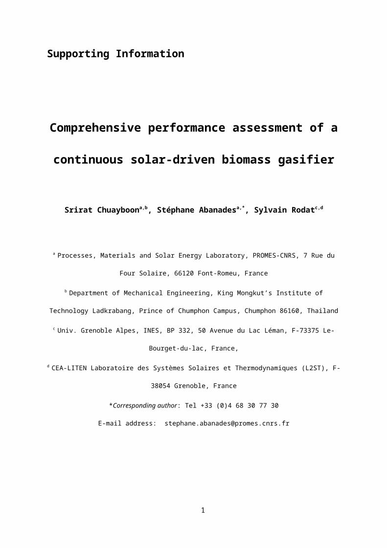
Fig. S2 shows the evolution of temperatures during heating phase and during biomass

injection.The homogeneous temperature and low gradient in the reaction zone is confirmed

by a small gap between T1 and T3, while Tpyrometer is lower as a result of the selected slightly

over-estimated emissivity (=1) for the cavity (Fig.S2a). A small temperature decrease is

observed after biomass injection due to the endothermal reaction while the cavity pressure

slightly increases because of the gas production (chemical expansion) due to the gasification

reaction. The syngas species production rates are continuously measured in the outlet gas.

During biomass injection (Fig.S2b), the solar power input was decreased step by step by

closing the shutter after 2, 5 and 15 min for stabilizing the operating temperature at 1300 °C

throughout the test, while the DNI remained constant at ~1000 W/m2.

3

Fig. S2. (a) Pressure, temperatures and syngas species evolution during heating phase and

feedstock injection, (b) solar power input and DNI evolution during feedstock injection

period (Run No.12)

4

3. Typical evolution of syngas production rates during continuous biomass injection

Fig. S3 presents a representative experiment of steam gasification with continuous biomass

injection. For this experiment, a total of 30 g of biomass type A was introduced at a biomass

feeding rate of ~2.2 g/min (~15 minutes of injection time) while the steam was set at 300

mg/min throughout the test, resulting in a H2O/biomass molar ratio of 2.1 (slightly over-

stoichiometric ratio). The experiment was carried out at a temperature of 1300 °C. The GC

measurements at different sampling times are also plotted (dots) to confirm and compare the

consistency of experimental results obtained from the online gas analyzer. The resulting

syngas production rates measured by the two techniques matched well. Stable patterns in the

flow-rates of H2 and CO were achieved during biomass injection, while CO2 and CH4 flow-

rates were also stable throughout the experiment, thus confirming stable biomass feeding rate

injection. The production rates of secondary hydrocarbons (CnHm) measured by GC include

the C2H2, C2H4, and C2H6 (the latter being in negligible amounts) (Fig. S4).

5

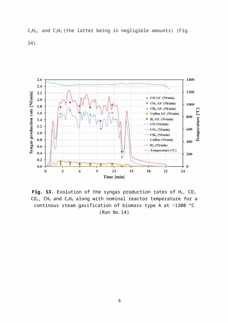
Fig. S3. Evolution of the syngas production rates of H2, CO, CO2, CH4 and CnHm along with nominal reactor temperature for a continous steam gasification of biomass type A at ~1300

°C (Run No.14)

Fig. S4. Evolution of C2H2, C2H4, and C2H6 production rates from GC measurements for a continuous steam gasification of biomass type A at 1300 °C (Run No.14).

6

4. Operating conditions and solar reactor performances assessment

A summary of the operating conditions and experimental results for 64 experimental runs of

the continuously-fed solar reactor are shown in Table S1. Solar-driven experiments were

carried out with five biomass feedstocks in a continuous process. The solar reactor was

operated under the following range of parameters: biomass feeding rates: 0.6-2.7 g/min,

H2O/biomass molar ratio: 1.6-7 (accounting for the initial moisture content in the biomass

feedstocks), carrier gas flow rate: 2-3.3 Nl/min, reactor temperature: 1100-1300 °C and solar

power input: 0.86-1.44 kW in order to optimize the synthesis gas production and assess the

performances of the solar biomass gasifier.

In this table, the different solar reactor performances are also highlighted related to the

energy upgrade factor (U), thermochemical reactor efficiency (reactor), solar-to-fuel energy

conversion efficiency (solar-to-fuel), and carbon conversion (XC) whether or not accounting for

the calorific value of C2H2 and C2H4 (total amount noted as C2Hm) in the produced syngas

obtained from GC measurements. If accounting for C2Hm, the values of U, solar-to-fuel and XC

are consistently increased.

Table S1. Operating conditions and experimentally measured performances of the solar reactor during continuous operation

Run #

Biomasstype

mfeedstock(g/min)

mH 2 O(mg/min)

H 2Ofeedstock

mAr(Nl/min)

T3

(°C)Qsolar

(kW)

ηreactor(%)

τ(sec)

Not accounting for C2H2 and C2H4

Accounting for C2H2 and C2H4

U ηsolar−¿− fuel(%)

Xc

(%) U ηsolar−¿− fuel(%)

Xc

(%)

1 Type A 1.2 200 2.3 3.3 1100 0.89 18.2 0.83 0.9

1 13.3 79.2

1.03 15.1 83.

7

2 Type A 1.5 200 2.1 3.3 1100 0.93 24.1 0.77 0.9

5 20.4 79.8

1.05 22.4 83.

1

3 Type A 1.2 200 2.3 2.7 1200 1.08 20.2 0.98 0.9

7 18.1 78.8

1.04 19.5 81.

5

4 Type A 1.5 200 2.1 2.7 1200 1.09 20.6 0.61 1.0

1 19.3 80.0

1.10 20.9 83.

2

5 Type A 1.5 200 2.1 3.3 1200 1.16 17.9 0.85 1.0

1 15.7 83.8

1.11 17.3 87.

4

6 Type A 1.8 300 2.3 2.7 1200 1.15 21.7 0.63 1.0

3 20.6 82.7

1.12 22.4 85.

8

7 Type A 0.8 200 3 2.7 1300 1.20 15.3 0.96 0.9

4 12.4 75.0

0.99 13.0 77.

0

8 Type A 1.2 200 2.3 2.7 1300 1.22 18.3 0.76 1.0

4 17.3 80.4

1.08 18.0 82.

59 Type A 1.5 200 2.1 2 130 1.22 17.3 0.95 1.1 19.4 86. 1.1 19.9 87.

7

0 4 2 7 7

10 Type A 1.5 200 2.1 2.3 1300 1.27 18.5 0.79 1.0

8 18.9 85.0

1.14 20.0 87.

3

11 Type A 1.5 200 2.1 3.3 1300 1.22 17.7 0.74 1.0

5 15.5 84.8

1.14 16.9 88.

2

12 Type A 1.8 200 1.8 2.7 1300 1.28 20.1 0.59 1.1

0 20.8 84.2

1.15 21.8 86.

4

13 Type A 2.2 200 1.6 2.7 1300 1.25 20.1 0.59 1.0

3 19.4 80.3

1.13 21.2 83.

9

14 Type A 2.2 300 2.1 2.7 1300 1.34 23.9 0.54 1.1

2 25.1 85.7

1.17 26.1 87.

7

15 Type A 2.2 500 2.8 2.7 1300 1.33 24.9 0.53 1.1

0 24.6 85.4

1.17 26.3 88.

3

16 Type A 2.5 400 2.2 2.7 1300 1.43 24.7 0.48 1.1

3 25.1 88.3

1.18 26.3 90.

2

17 Type A 2.7 450 2.3 2.7 1300 1.44 25.3 0.47 1.1

4 26.6 88.6

1.19 27.8 90.

4

18 Type B 1.2 200 2.3 2.7 1100 1.03 16.1 0.83 0.9

3 13.6 78.5

1.01 14.7 81.

2

19 Type B 1.2 500 4.5 2.7 1100 1.01 23.1 0.84 0.9

6 18.9 80.6

1.09 21.5 85.

2

20 Type B 0.8 500 6.4 2.7 1200 1.13 19.4 0.85 1.0

0 15.9 81.1

1.07 17.0 83.

8

21 Type B 1.2 163 2 2.7 1200 1.13 18.2 0.74 0.9

9 16.8 78.4

1.09 18.5 82.

0

22 Type B 1.2 200 2.3 2 1200 1.12 17.4 0.87 1.0

6 17.8 84.1

1.10 18.5 85.

9

23 Type B 1.2 200 2.3 2.7 1200 1.16 18.6 0.68 1.0

1 17.7 81.0

1.07 18.7 83.

3

24 Type B 1.2 200 2.3 3.2 1200 1.16 20.3 0.67 0.9

8 18.1 78.6

1.08 19.9 82.

3

25 Type B 1.2 500 4.5 2.7 1200 1.18 21.0 0.74 1.0

1 18.1 81.3

1.08 19.4 83.

8

26 Type B 1.5 500 3.8 2.7 1200 1.20 24.5 0.71 1.0

2 22.3 81.4

1.08 23.7 83.

6

27 Type B 1.8 500 3.3 2.7 1200 1.20 24.9 0.69 1.0

2 22.8 81.8

1.11 24.6 84.

7

28 Type B 0.8 140 2.4 2.7 1300 1.17 17.3 0.78 0.9

9 15.7 78.7

1.03 16.3 80.

3

29 Type B 1.2 200 2.3 2.7 1300 1.23 17.5 0.67 1.0

3 17.5 78.6

1.08 18.3 80.

8

30 Type B 1.2 500 4.5 2.7 1300 1.22 20.7 0.70 1.0

3 20.4 81.5

1.07 21.2 83.

4

31 Type B 1.8 250 2 2.7 1300 1.24 23.6 0.58 1.0

9 24.0 83.1 1.1 25.0 85.

1

32 Type B 2.2 300 2 2.7 1300 1.29 24.2 0.52 1.1

0 25.0 84.2

1.15 26.0 86.

1

33 Type C 1.2 200 2.1 2.7 1100 0.86 17.5 0.85 0.9

1 16.1 71.7

1.05 18.5 76.

3

34 Type C 1.2 200 2.1 2.7 1200 1.08 18.7 0.78 1.0

1 16.6 75.8

1.09 17.9 78.

6

35 Type C 1.5 250 2.1 2.7 1200 1.09 19.6 0.73 1.0

3 17.5 79.2

1.10 18.7 81.

6

36 Type C 1.8 300 2.1 2.7 1200 1.10 26.5 0.61 1.1

0 26.5 81.5

1.17 28.2 83.

7

37 Type C 2.2 350 2.1 2.7 1200 1.15 27.1 0.55 1.1

1 26.8 82.3

1.21 29.2 85.

6

38 Type C 1.2 200 2.1 2.7 1300 1.21 17.9 0.71 1.0

4 16.2 75.4

1.09 17.0 77.

5

39 Type C 1.5 200 1.8 2.7 1300 1.22 20.0 0.54 1.1

2 19.8 79.1

1.17 20.8 81.

4

40 Type C 1.8 300 2.1 2.7 1300 1.25 22.4 0.57 1.1

3 22.4 80.7

1.19 23.6 83.

0

41 Type C 2.2 350 2.1 2.7 1300 1.26 26.5 0.54 1.1

4 26.7 81.1

1.20 28.1 83.

3

42 Type C 2.5 450 2.2 2.7 1300 1.30 27.0 0.51 1.1

6 27.6 84.0

1.22 29.0 86.

1

43 Type C 2.7 500 2.3 2.7 1300 1.43 24.2 0.51 1.1

4 24.3 84.3

1.24 26.4 87.

6

44 Type D 0.8 200 3.3 2.7 1100 0.89 16.4 0.95 0.9

7 14.0 77.5

1.06 15.2 80.

3

45 Type D 1.2 200 2.5 3.3 1100 0.87 17.5 0.76 0.9

7 13.1 75.5

1.06 14.3 78.

9

46 Type D 0.8 200 3.3 2.7 1200 1.03 15.8 0.92 1.0

2 13.6 78.5

1.07 14.2 80.

5

47 Type D 1.2 200 2.5 2.7 1200 1.18 20.3 0.65 1.0

6 20.4 79.5

1.11 21.4 81.

3

48 Type D 1.2 200 2.5 3.3 1200 1.15 14.9 0.66 0.9

9 11.8 77.0

1.04 12.4 79.

0

49 Type D 1.8 450 3.3 2.7 1200 1.15 26.5 0.64 1.0

7 25.4 79.2

1.13 26.8 81.

2

50 Type D 0.8 200 3.3 2.7 1300 1.17 16.1 0.81 1.0

7 14.8 76.4

1.12 15.5 78.

6

8

51 Type D 1.2 360 3.8 2.7 1300 1.29 19.9 0.66 1.1

3 20.0 80.6

1.18 20.8 82.

4

52 Type D 1.2 200 2.5 3.3 1300 1.20 16.9 0.68 1.0

2 17.5 73.3

1.06 18.3 75.

1

53 Type D 1.5 450 3.8 2.7 1300 1.27 22.3 0.61 1.1

4 22.4 80.3

1.20 23.6 82.

4

54 Type D 1.8 500 3.6 2.7 1300 1.30 22.6 0.60 1.2

0 23.4 84.9

1.24 24.3 86.

7

55 Type D 2.2 500 3.1 2.7 1300 1.43 24.0 0.58 1.1

6 25.3 82.7

1.20 26.3 84.

3

56 Type E 0.8 500 7 2.7 1100 0.98 19.4 0.95 1.0

0 15.4 72.9

1.10 17.0 76.

2

57 Type E 1.2 300 3.3 2.7 1100 0.99 17.4 0.86 1.0

3 14.6 74.8

1.14 16.2 78.

3

58 Type E 0.6 200 4.1 2.7 1200 1.07 15.0 1.02 0.9

8 11.8 69.9

1.02 12.3 71.

7

59 Type E 0.8 200 3.3 2.7 1200 1.08 16.0 0.88 1.0

0 13.7 70.6

1.05 14.4 72.

6

60 Type E 1.2 300 3.3 2.7 1200 1.12 19.5 0.81 1.1

1 18.7 76.3

1.15 19.4 78.

0

61 Type E 1.5 350 3.2 2.7 1200 1.13 20.4 0.70 1.1

5 20.0 80.6

1.20 20.8 82.

4

62 Type E 0.8 200 3.3 2.7 1300 1.19 15.7 0.82 1.1

3 15.0 77.0

1.16 15.4 78.

3

63 Type E 1.2 300 3.3 2.7 1300 1.28 19.0 0.80 1.1

2 16.6 76.1

1.14 16.9 77.

4

64 Type E 1.5 350 3.2 2.7 1300 1.24 21.2 0.67 1.1

5 21.2 76.7

1.19 21.8 78.

2

The U values were in the ranges of 0.91-1.14, 0.93-1.10, 0.91-1.16, 0.97-1.20 and 0.98-1.15

for biomass types A, B, C, D and E, respectively. When accounting for C2Hm, the U (C2Hm)

values were in the ranges of 1-1.19, 1.01-1.15, 1.05-1.24, 1.04-1.24 and 1.02-1.20 for

biomass types A, B, C, D and E, respectively. A few experiments show the value of U below

one, especially at both the lowest operating temperature or at the lowest biomass feeding

rates due to low reaction kinetics. However, when accounting for the calorific value of C2Hm,

all of the U values are above one. On the one hand, the values of U lower than one mean that

the solar energy was not stored efficiently in the chemical form and the upgrading of the

calorific value of the feedstock was not successful. On the other hand, the values of U higher

than one indicate that the solar energy was successfully stored in chemical form and the

calorific value of the feedstock was upgraded by the solar gasification process.

Table S2 compares the highest energy upgrade factor at 1300 °C to the theoretical maximum

values attained at the thermodynamic equilibrium reached above 1000 °C when assuming

complete biomass conversion into H2 and CO species. Considering the U values when

accounting for C2Hm, biomass type A shows the highest percentage of U achieved as

compared to equilibrium (93%).

9

Table S2. Comparison of highest energy upgrade factor to theoretical one based on equilibrium

Type Run No. mfeedstock(g/min)

T3

(°C)

Energy upgrade factor (U)

Theoretical U U

U(accounting for C2Hm)

% of maximum achievable

valueType A 17 2.7 1300 1.28 1.14 1.19 93Type B 32 2.2 1300 1.28 1.10 1.15 90Type C 42 2.5* 1300 1.40 1.16 1.22 87Type D 54 1.8* 1300 1.44 1.20 1.24 86Type E 64 1.5 1300 1.44 1.15 1.19 83

*at optimal biomass feeding rate

Note that the conventional autothermal gasification achieves the U value of approximately

0.7 depending on feedstock (Wieckert et al., 2013)1, as a result of a significant portion of the

feedstock being combusted for supplying process heat to the endothermic reaction. The

calorific value of the produced syngas was solar upgraded by 15-24% with respect to the

feedstock, thus highly outperforming the U obtained from conventional autothermal

gasification process.

The solar-to-fuel varies in the ranges of 12.4-26.6%, 13.6-25.0%, 16.1-27.6%, 11.8-25.4% and

11.8-21.2% for biomass types A, B, C, D and E, respectively. When accounting for C2Hm, the

values in the ranges of 13.0-27.8%, 14.7-26.0%, 17.0-29.2%, 12.4-26.8% and 12.3-21.8%

were achieved. The lowest solar-to-fuel were found at low biomass feeding rates as a result of

inefficient utilization of the solar energy and limited syngas production, at the expense of

higher heat losses. Obviously, increasing biomass feeding rate significantly enhanced the

solar-to-fuel. Conversely, excessively high biomass feeding rate reduced the solar-to-fuel. Thus,

optimal biomass feeding rate was evidenced for achieving maximum reactor performance as

well as syngas production.

1 Wieckert, C., Obrist, A., Zedtwitz, P. von, Maag, G., Steinfeld, A., 2013. Syngas Production by Thermochemical Gasification of Carbonaceous Waste Materials in a 150 kW th Packed-Bed Solar Reactor. Energy & Fuels 27, 4770–4776.

10

Likewise, the reactor increased with biomass feeding rate ranging between 15.3-25.3

%, 16.1-24.9%, 17.5-27.1%, 14.9-26.5% and 15-21.2% for biomass types A, B, C, D and E,

respectively. The lowest reactor values were observed at the lowest biomass feeding rate,

meaning that high heat losses occurred because of the extended biomass injection duration

(for the same amount of feedstock injected). Increasing the biomass feeding rate inherently

reduced the processing duration (for a given amount of biomass) and thus the amount of solar

energy absorbed by the reactor, which in turn drastically enhanced the reactor efficiency with

maximum values typically above 25%. Based on all of the experimental results, the peak

values of the performance indicators achieved were: U=1.24 obtained for biomass types C

and D, solar-to-fuel = 29.2 % obtained for biomass type C, XC= 90.4% obtained for biomass type

A, reactor = 27.1% obtained for biomass type C.

11

5. Steam mass flow-rate chart for a stoichiometric H2O/biomass molar ratio

Fig.S5 displays the relative mass flow rates of steam and biomass feedstock for a

stoichiometric ratio (accounting for the moisture content in the feedstock). These curves were

used for determining the required steam flow rate when either adjusting biomass feeding rate

or changing biomass type.

Fig. S5. Relation between the mass flow rates of steam and biomass feedstocks for a

stoichiometric ratio (H2O/biomass molar ratios of 2 for biomass types A, B and C and 3 for

biomass types D and E)

12

6. Window deposit due to the presence of smoke at low temperature

Fig.S6 shows the dirt on the window as a result of smoke release during gasification process

at 1100 °C.

Fig. S6. Dirt deposits on the window observed at low temperature (1100°C)

7. Effect of temperature on syngas yield and energy upgrade factor

Additional experiments (Fig.S7) were carried out to validate the effect of temperature (1100-

1300 ºC) on syngas production and energy upgrade factor (U). The biomass feeding rates

were 1.5 g/min for biomass type A (Fig.S7a) and 1.2 g/min for biomass types B (Fig.S7b)

and D (Fig.S7c). Ar and steam flow rates were fixed (3.3 Nl/min and 200 mg/min for

biomass types A and D, 2.7 Nl/min and 500 g/min for biomass type B, respectively).

The results confirm that an increase in the temperature promoted total syngas yield,

regardless of operating conditions and biomass types (Fig.S7). H2 and CO yields increased

while C2Hm, CH4, and CO2 yields decreased with increasing temperature. Moreover, a

substantial enhancement of the syngas yield consistent with temperature led to an increase in

U. It can be noticed that a higher C2Hm production occurred when reducing temperature,

which in turn increased U(C2Hm) because of the high calorific value of C2Hm.

13

Fig. S7. Temperature influence on syngas yields and energy upgrade factors for biomass types A (a), B (b), and D (c)

14

8. Kinetic study

The Arrhenius plot is generally utilized to evaluate the influence of temperature on the rates

of chemical reactions.

k=A ∙exp (−Ea/ RT ) (S1)

Where k is the reaction rate constant, A is the pre-exponential factor, Ea is the

activation energy, R is the gas constant and T is the absolute temperature.

In this study, the reaction rate constants (k) were obtained for each biomass type and

temperatures from the average nominal syngas production rates of H2 and CO at steady state,

which are the main gaseous species contained in the produced syngas during continuous

biomass feeding. The logarithm evolution of the reaction rates versus inverse temperature

(Eq.S1) was subsequently plotted from 1100 to 1300 °C, and the values of activation energy

(Ea) for each biomass type were consequently obtained as presented in Fig. S8. A significant

effect of the temperature on the production rates of H2 and CO was observed. The Ea for

different biomass types were determined to be in the ranges of 23.7-28.8 kJ/mol based on H2

and 24.3-29.5 kJ/mol based on CO, according to Table S3. Thus, the Ea values obtained from

H2 and CO production rates are very similar, and they increased consistently with biomass

particle size (larger particles size implies higher Ea).

15

Fig.S8. Arrhenius plot based on H2 and CO production rates for biomass types A (a), B (b), C

(c), D (d) and E (e) at 1100-1300 °C (biomass feeding rate of 1.2 g/min)

16

Table S3. Activation energy related to the H2 and CO production rates obtained by Arrhenius plot

Biomass type Gaseous Specie Ea

(kJ/ mol)Type A(1 mm)

H2 26.5±3CO 27.5±3

Type B(4 mm)

H2 28.8±4CO 29.5±4

Type C(0.55 mm)

H2 25.6±3CO 27.3±3

Type D(0.30 mm)

H2 23.7±4CO 24.3±4

Type E(2 mm)

H2 25.9±5CO 26.1±5

9. Ashes remaining in the reactor cavity

Fig.S9 shows the presence of ashes remaining inside the reactor cavity (brown color particles

covering the black SiC particles), which decreased when increasing the temperature from

1100 °C to 1300 °C. This indicates that ashes were presumably melted when the temperature

increased, which may in turn favor the corrosion of the cavity walls (because of the presence

of alkali metal chlorides) in accordance with the black circles on the wall surface (note that

the cavity bottom was filled with SiC particles to avoid the trickling of melted ashes that may

clog the gas inlet).

Fig.S9. Ashes remaining inside the reactor cavity for biomass type A at (a) 1100 °C, (b) 1200

°C, and (c) 1300 °C (same amount of biomass injected, 30 g)

17

10. Effect of biomass feeding rate for each biomass type at 1200 °C

The results of biomass feeding rate influence at 1200 °C on syngas production are presented

separately according to the different biomass types.

Concerning biomass type A (Fig. S10), the C2Hm, CH4 and CO2 mole fractions increased, the

CO mole fraction decreased, and the H2 mole fraction appeared to be stable when increasing

biomass feeding rate (Fig. S10a). The CO quantity decreased slightly while the H2, C2Hm,

CH4 and CO2 quantities increased with biomass feeding rate (Fig. S10b), which resulted in

the increase of the total syngas yield, from 64.8 mmol/gbiomass at 1.2 g/min to 68.6 mmol/gbiomass

at 1.8 g/min. Thus, increasing biomass feeding rate hastens the gasification rate and improves

the syngas production. However, the increase of biomass feeding rate has an adverse effect

on the residence time that is reduced from 0.98 s at 1.2 g/min to 0.63 s at 1.8 g/min, which

promotes the increase of C2Hm, CH4 and CO2. In comparison to 1300 °C (biomass type A), H2

and CO yields were lower while the C2Hm, CH4 and CO2 yields were higher at 1200 °C,

because of the lower gasification kinetics. U increased with biomass feeding rate with the

highest value of 1.03 (1.12 when accounting for C2Hm) at 1.8 g/min.

18

Fig. S10. Influence of biomass feeding rate for biomass type A on (a) average syngas

composition, (b) syngas yield and energy upgrade factor at 1200 °C

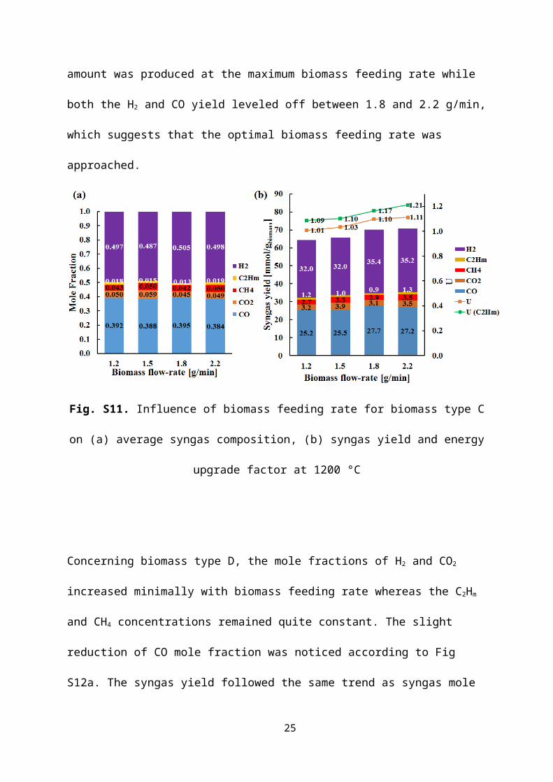
Regarding biomass type C (Fig. S11a), the H2 mole fraction shows no biomass feeding rate

dependency similarly to biomass type A. The reduction of CO mole fraction and the increase

of C2Hm and CH4 mole fractions with biomass feeding rate is also explained by the decline of

the gas residence time. According to Fig.S11b, the syngas yields increased with biomass

feeding rate indicating that increasing biomass feeding rate led to higher biomass

consumption rate and higher syngas yield, thereby leading to the improvement of U ranging

between 1.01 and 1.11 (1.09-1.21 when accounting for C2Hm). The maximum C2Hm amount

was produced at the maximum biomass feeding rate while both the H2 and CO yield leveled

off between 1.8 and 2.2 g/min, which suggests that the optimal biomass feeding rate was

approached.

19

Fig. S11. Influence of biomass feeding rate for biomass type C on (a) average syngas

composition, (b) syngas yield and energy upgrade factor at 1200 °C

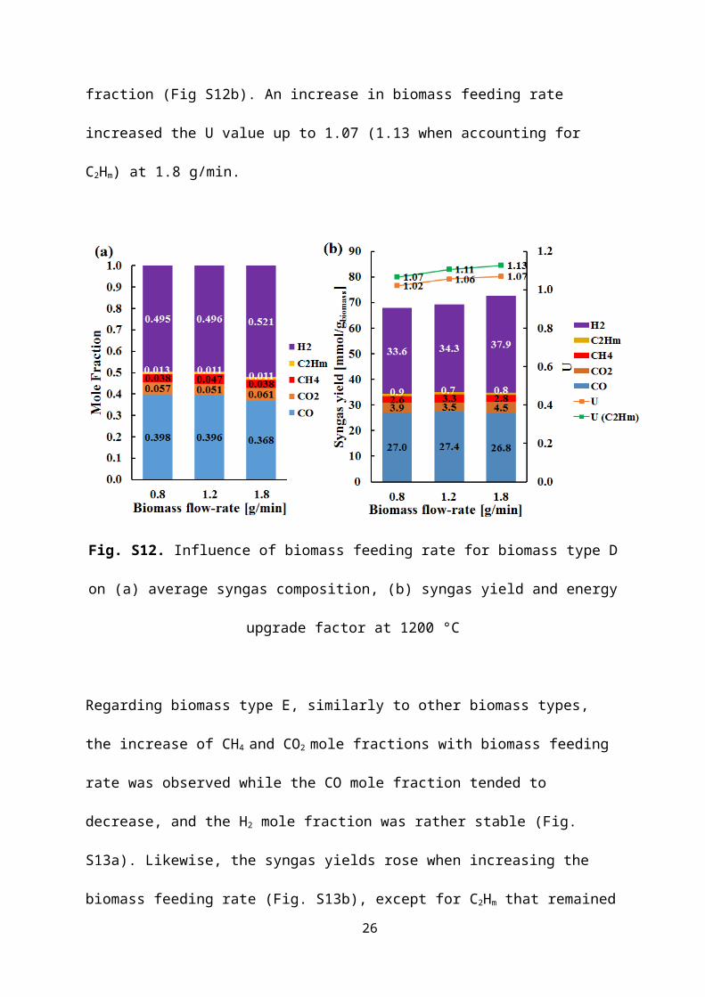
Concerning biomass type D, the mole fractions of H2 and CO2 increased minimally with

biomass feeding rate whereas the C2Hm and CH4 concentrations remained quite constant. The

slight reduction of CO mole fraction was noticed according to Fig S12a. The syngas yield

followed the same trend as syngas mole fraction (Fig S12b). An increase in biomass feeding

rate increased the U value up to 1.07 (1.13 when accounting for C2Hm) at 1.8 g/min.

20

Fig. S12. Influence of biomass feeding rate for biomass type D on (a) average syngas

composition, (b) syngas yield and energy upgrade factor at 1200 °C

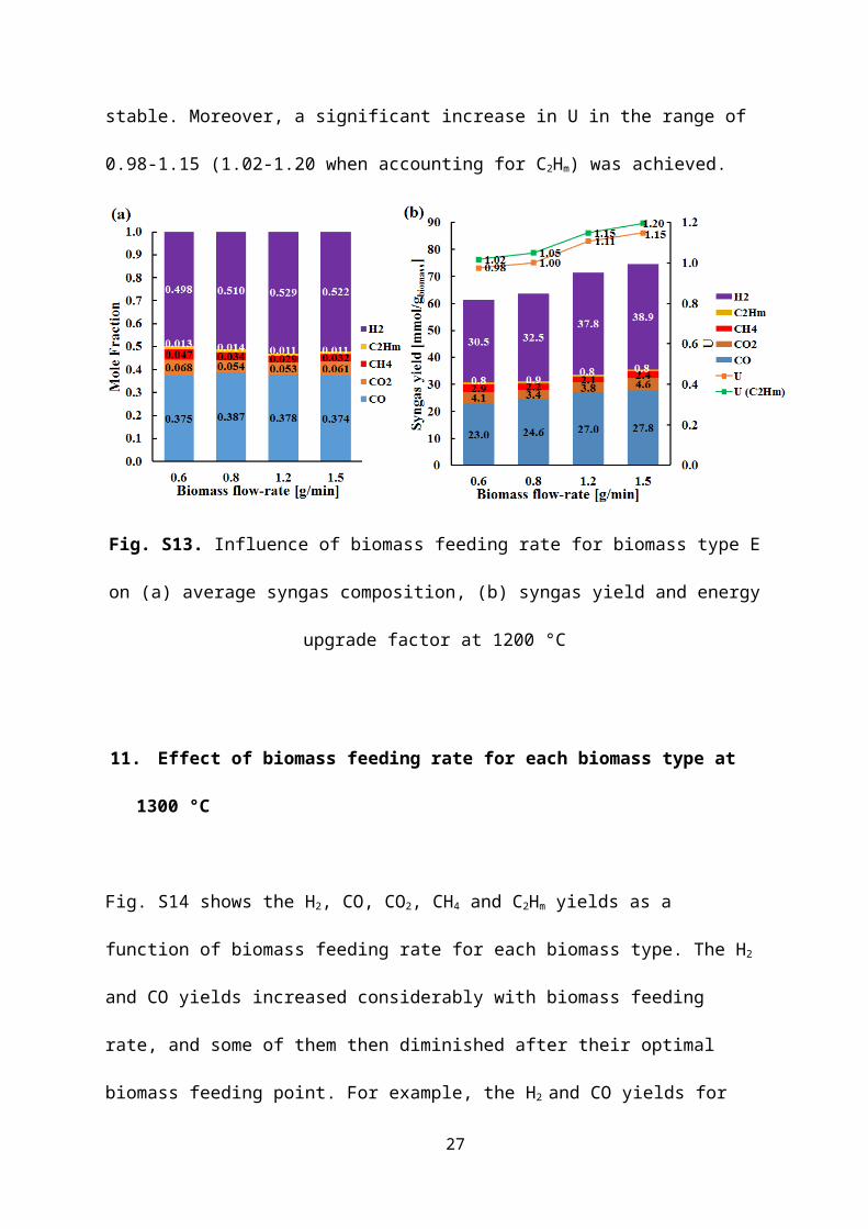
Regarding biomass type E, similarly to other biomass types, the increase of CH4 and CO2

mole fractions with biomass feeding rate was observed while the CO mole fraction tended to

decrease, and the H2 mole fraction was rather stable (Fig. S13a). Likewise, the syngas yields

rose when increasing the biomass feeding rate (Fig. S13b), except for C2Hm that remained

stable. Moreover, a significant increase in U in the range of 0.98-1.15 (1.02-1.20 when

accounting for C2Hm) was achieved.

21

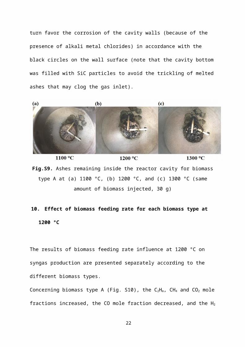
Fig. S13. Influence of biomass feeding rate for biomass type E on (a) average syngas

composition, (b) syngas yield and energy upgrade factor at 1200 °C

11. Effect of biomass feeding rate for each biomass type at 1300 °C

Fig. S14 shows the H2, CO, CO2, CH4 and C2Hm yields as a function of biomass feeding rate

for each biomass type. The H2 and CO yields increased considerably with biomass feeding

rate, and some of them then diminished after their optimal biomass feeding point. For

example, the H2 and CO yields for biomass type C reached the maximum value of 39.2 and

29.1 mmol/gbiomass at 2.5 g/min and then reduced to 37.6 and 27.9 mmol/gbiomass, respectively,

at 2.7 g/min. Similarly, with the increase of biomass feeding rate, the amounts of CO2 and

CH4 for biomass type C increased in the ranges of 2.5-4.0 and 1.7-3.2 mmol/gbiomass,

respectively, while the C2Hm yields increased slightly in the range of 0.9-1.4 mmol/gbiomass.

Increasing the biomass feeding rate promoted syngas yield; however, an increase in CO2, CH4

and C2Hm yields due to a lowered gas residence time led to a negative impact on syngas

quality. Small fluctuation in the CO2 yields (Fig. S14c) is attributed to temporal changes in

22

the H2O/biomass ratio, which influences water-gas shift reaction (CO+H2O→CO2+H2),

because of transient variations in feedstock delivery. Similar trends of H2 yield between

biomass types A and B and between biomass types D and E were observed thanks to their

similar initial chemical composition. The H2 yields for biomass types D and E were higher

than the other types owing to their higher initial hydrogen content in the feedstock.

Fig. S14. Influence of biomass feeding rate on syngas yield for different biomass feestocks at 1300 °C

23

12. Influence of biomass feeding rate on syngas production rates evolution

The biomass feeding rate influence on syngas production rates evolution at 1300 °C are

presented in Fig. S15 (biomass type A). It is clear that increasing biomass feeding rate both

increased syngas production rates and decreased the operating duration time, thus improving

both syngas yield and reactor performances (reduced heat losses). For instance, the biomass

injection duration decreased significantly from 40-45 min at ~0.8 g/min to 11-18 min at ~2.7

g/min, while the nominal H2 and CO production rates were 0.6 and 0.5 Nl/min at 0.8 g/min

compared to 2.4 and 2 Nl/min at 2.7 g/min respectively.

Fig. S15. Biomasss feeding rate influence on (a) H2, (b) CO, (c) CH4 and (d) CO2 production rates during gasification at 1300 °C (Biomass type A)

24

13. Energy balance

Fig. S16 shows the solar power consumption as a function of biomass feeding rate for

biomass type E at 1200 °C. An increase in biomass feeding rate led to the growth of solar

power consumption devoted to chemical reaction (Qreaction), steam heating (Qwater) and

biomass heating (Qbiomass) from 0.077, 0.016 and 0.018 kW at 0.6 g/min to 0.125, 0.026 and

0.030 kW at 1.5 g/min respectively, thus increasing the total solar power consumption from

0.160 kW at 0.6 g/min to 0.231 kW at 1.5 g/min. The solar power input was thus increased in

the range 1.07-1.13 kW to stabilize the temperature at 1200 °C. The amount of solar power

devoted to inert gas heating (QAr) remained stable (~0.050 kW) as its flow rate was kept

constant at 2.7 Nl/min throughout the tests. Thus, the sensible heat losses associated with the

energy for inert gas heating were considerably reduced when increasing biomass feeding rate

as a result of a shortened processing duration.

Fig. S16. Solar power consumption for biomass type E at 1200 °C

The energy partition for the solar reactor given as percentage of the average solar power input

throughout the experimental tests for biomass type E at 1200 °C is presented in Fig. S17.

25

Obviously, increasing the biomass feeding rate decreased the heat losses from 85.0% at 0.6

g/min to 79.6% at 1.5 g/min, thereby enhancing the utilization of solar energy input.

Fig. S17. Energy partition for the solar reactor given as percentage of the solar power input

averaged over the entire experimental test at 1200 °C (biomass type E)

14. Comparison of the carbon consumption rate at different temperatures as a function

of biomass feeding rate

Fig.S18 shows the carbon consumption rate as a function of the carbon feeding rate at 1100,

1200, and 1300 °C for biomass types A, C and D compared to the ideal carbon consumption

rate for each biomass type (equal to the carbon feeding rate, i.e. the carbon contained in the

fed biomass). The carbon consumption rate increased with the biomass feeding rate. It was

quantified by the summation of the nominal rates of CO, CO2, and CH4 production contained

in the produced syngas (assuming that C consumption rate and the summation of production

rates of carbon-containing gas species are equivalent) and achieved during continuous

26

biomass injection (at steady state). Typically, the carbon consumption rate closely followed

the carbon feeding rate at low feeding rates, which means that the reactant feeding rate

closely matched the rate of the gasification reaction. From a threshold value of carbon

feeding rate (at 1300°C), the carbon consumption rate became lower than the carbon feeding

rate (e.g., 0.8 g/min for biomass type A), which means that the gasification rate is not high

enough to convert totally the injected biomass. In other words, from this point, carbon

accumulation in the reactor (due to incomplete biomass gasification) may occur if the feeding

rate is too high with respect to the reactor capacity. An optimal value was observed for

biomass type C at a carbon feeding rate of 1.16 g/min (1300 °C). Both the carbon

consumption rates and carbon feeding ranges at 1300 °C were higher and closer to the ideal

carbon consumption rates for any biomass type compared to those obtained at 1100 and 1200

°C. This is because the higher gasification kinetics at 1300 °C resulted in both higher carbon

consumption rate and carbon feeding range. The impact of biomass feeding rate on syngas

production capacity and reactor performances was thus evidenced. The carbon consumption

rate at 1300°C matched closely the carbon feeding rate (provided the feeding rate was below

a threshold value regardless of the biomass type). This means that 1300°C is a suitable

temperature to operate reliably the solar biomass gasifier in a continuous mode with a

biomass conversion rate equal to the feeding rate.

27

Fig. S18. Comparison of the effect of biomass feeding rate and temperature on carbon consumption rate for biomass types A (a), C (b) and D (c) at 1100, 1200, and 1300 °C

28