AROUND THE BOUNDARY OF COMPLEX DYNAMICS.

AROUND THE BOUNDARY OF COMPLEX DYNAMICS.

ROLAND K.W. ROEDER

Abstract. We introduce the exciting field of complex dynamics atan undergraduate level while reviewing, reinforcing, and extending theideas learned in an typical first course on complex analysis. Julia setsand the famous Mandelbrot set will be introduced and interesting prop-erties of their boundaries will be described. We will conclude with adiscussion of problems at the boundary between complex dynamics andother areas, including a nice application of the material we have learnedto a problem in astrophysics.

Preface

These notes were written for the 2015 Thematic Program on Boundariesand Dynamics held at Notre Dame University. They are intended for anadvanced undergraduate student who is majoring in mathematics. In anideal world, a student reading these notes will have already taken under-graduate level courses in complex variables, real analysis, and topology. Asthe world is far from ideal, we will also review the needed material.

There are many fantastic places to learn complex dynamics, including thebooks by Beardon [3], Carleson-Gamelin [10], Devaney [11, 12], Milnor [37],and Steinmetz [46], as well as the Orsay Notes [13] by Douady and Hubbard,the surveys by Blanchard [5] and Lyubich [32, 31], and the invitation totranscendental dynamics by Shen and Rempe-Gillen [44]. The books byDevaney and the article by Shen and Rempe-Gillen are especially accessibleto undergraduates. We will take a complementary approach, following asomewhat different path through some of the same material as presentedin these sources. We will also present modern connections at the boundarybetween complex dynamics and other areas.

None of the results presented here are new. In fact, I learned most ofthem from the aforementioned textbooks and from courses and informaldiscussions with John Hubbard and Mikhail Lyubich.

Our approach is both informal and naive. We make no effort to providea comprehensive or historically complete introduction to the subject. Manyimportant results will be omitted. Rather, we will simply have fun doingmathematics.

1

arX

iv:1

506.

0711

3v2

[m

ath.

DS]

15

Aug

201

5

2 ROLAND K.W. ROEDER

Dedicated to Emile and Eli.

Acknowledgments I am grateful to Notre Dame University for their hos-pitality during the thematic program on boundaries and dynamics. IvanChio, Youkow Homma, Lyndon Ji, Scott Kaschner, Dmitry Khavinson,Seung-Yeop Lee, Rodrigo Perez, and Mitsuhiro Shishikura provided manyhelpful comments. All of the computer-drawn images of basins of attrac-tion, filled Julia sets, and the Mandelbrot set were created using the Frac-talstream software [19] that was written by Matthew Noonan. This workwas partially supported by NSF grant DMS-1348589.

Lecture 1: “Warm up”

Let us start at the very beginning:

1.1. Complex Numbers. Recall that a complex number has the formz = x + iy, where x, y ∈ R and i satisfies i2 = −1. One adds, subtracts,multiplies, and divides complex numbers using the following rules:

(a+ bi)± (c+ di) = (a± c) + (b± d)i,

(a+ bi)(c+ di) = ac+ adi+ bci+ bdi2 = (ac− bd) + (ad+ bc)i, and

a+ bi

c+ di=a+ bi

c+ di

c− dic− di

=(ac+ bd) + (bc− ad)i

c2 + d2.

The set of complex numbers forms a field C under the operations of additionand multiplication.

The real part of z = x + iy is Re(z) = x and the imaginary part ofz = x + iy is Im(z) = y. One typically depicts a complex number in thecomplex plane using the horizontal axis to measure the real part and thevertical axis to measure the imaginary part; See Figure 1. One can also takethe real or imaginary part of more complicated expressions. For example,Re(z2) = x2 − y2 and Im(z2) = 2xy.

The complex conjugate of z = x+ iy is z = x− iy and the modulus

of z is |z| =√x2 + y2 =

√zz. In the complex plane, z is obtained by

reflecting z across the real axis and |z| is the distance from z to the origin0 = 0 + 0i. The argument of z 6= 0 is the angle counterclockwise from thepositive real axis to z.

A helpful tool is the:

Triangle Inequality. For every z, w ∈ C we have

|z| − |w| ≤ |z + w| ≤ |z|+ |w|.

A complex polynomial p(z) of degree d is an expression of the form

p(z) = adzd + ad−1z

d−1 + · · ·+ a1z + a0

AROUND THE BOUNDARY OF COMPLEX DYNAMICS. 3

1

|z|

arg(z)

Im(z)

z = x− iy

z = x+ iy

x = Re(z)Re(z)

y = Im(z)

0

i

Figure 1. The complex plane.

where ad, . . . , a0 are some given complex numbers with ad 6= 0. Historically,complex numbers were introduced so that the following theorem holds:

Fundamental Theorem of Algebra. A polynomial p(z) of degree d hasd complex zeros z1, . . . , zd, counted with multiplicity.

In other words, a complex polynomial p(z) can be factored over thecomplex numbers as

p(z) = c(z − z1)(z − z2) · · · (z − zd),(1)

where c 6= 0 and some of the roots zj may be repeated. (The number oftimes zj is repeated in (1) is the multiplicity of zj as a root of p.)

Multiplying and dividing complex numbers is often simpler in polarform. Euler’s Formula states

eiθ = cos θ + i sin θ for any θ ∈ R.

We can therefore represent any complex number z = x + iy by z = reiθ

where r = |z| and θ = arg(z). Suppose z = reiθ and w = seiφ and n ∈ N.The simple formulae

zw = rsei(θ+φ), zn = rneinθ, andz

w=r

sei(θ−φ).(2)

follow from the rules of exponentiation. Multiplication and taking powersof complex numbers in polar form are depicted geometrically in Figure 2.


i

z = reiθ

z2 = r2ei2θ

0Re(z)

θ

Im(z)

1

z3 = r3ei3θ

θθ

θ

i

z4 = r4ei4θ

0

φθ

Re(z)

θ

zw = rsei(θ+φ)Im(z)

z = reiθ

1

w = seiφ

Figure 2. Multiplication and taking powers in polar form.

1.2. Iterating Linear Maps. A linear map L : C → C is a mappingof the form L(z) = az, where a ∈ C \ {0}. Suppose we take some initialcondition z0 ∈ C and repeatedly apply L:

z0// L(z0) // L(L(z0)) // L(L(L(z0))) // · · · .(3)

For any natural number n ≥ 1 let L◦n : C → C denote the composition ofL with itself n times. We will often also use the notation

zn := L◦n(z0).

The sequence {zn}∞n=0 ≡ {L◦n(z0)}∞n=0 is called the sequence of iterates ofz0 under L. It is also called the orbit of z0 under L.

Remark. The notion of linear used above is from your course on linearalgebra: a linear map must satisfy L(z +w) = L(z) +L(w) for all z, w ∈ Cand L(cz) = cL(z) for all z, c ∈ C. For this reason, mappings of the formz 7→ az + b are not considered linear. Instead, they are called affine.(See Exercise 1.)

The number a is called a parameter of the system. We think of it asdescribing the overall state of the system (think, for example, temperatureor barometric pressure) that is fixed for all iterates n. One can change theparameter to see how it affects the behavior of sequences of iterates (forexample, if the temperature is higher, does the orbit move farther in eachstep?).

Our rules for products and powers in polar form (2) allow us to under-stand the sequence of iterates (3). Suppose z0 = reiθ and a = seiθ withr, s > 0. Then, the behavior of the iterates depends on s = |a|, as shown inFigure 3.


|a| > 1 implies 0 is unstable

i

φφ

z3 = az2

i

Im(z)

a = seiφ

φ

z0 = reiθ

z3 = rs3ei(θ+3φ)

z4

z5

φ

φ

φ

1

z2 = rs2ei(θ+2φ)

z1 = rsei(θ+φ)

φφ

|a| < 1 implies 0 is stable

Re(z)

Re(z)

Im(z)

z4

1

z5

z0

φ

φ

z1 = az0

z2 = az1

a = seiφ

z7

z6

φφ

φ

φ

Figure 3. Iterating the linear map L(z) = az. Above:|a| < 1 implies orbits spiral into 0. Below: |a| > 0 implies sspiral away from 0. Not Shown: |a| = 1 implies orbits rotatearound 0 at constant modulus.

Remark. For a linear map L(z) = az with |a| 6= 1 the orbits {zn} and {wn}for any two non-zero initial conditions z0 and w0 have the same dynamicalbehavior. If |a| < 1 then

limn→∞

zn = 0 = limn→∞

wn

and if |a| > 1 then

limn→∞

zn =∞ = limn→∞

wn.


This is atypical for dynamical systems—the long term behavior of theorbit usually depends greatly on the initial condition. For example, we willsoon see that when iterating the quadratic mapping p(z) = z2 + i

4 thereare many initial conditions whose orbits remain bounded and many whoseorbit escapes to ∞. There will also be many initial conditions whose orbitshave completely different behavior! Linear maps are just too simple to haveinteresting dynamical properties.

Exercise 1. An affine mapping A : C → C is a mapping given by A(z) =az + b, where a, b ∈ C and a 6= 0. Show that iteration of affine mappingsproduces no dynamical behavior that was not seen when iterating linearmappings.

1.3. Iterating quadratic polynomials. Matters become far more inter-esting if one iterates quadratic mappings pc : C→ C given by pc(z) = z2+c.Here, c is a parameter, which we sometimes include in the notation by meansof a subscript, writing pc(z), and sometimes omit, writing simply p(z).

Remark. Like in Exercise 1, one can show that quadratic mappings ofthe form pc(z) = z2 + c actually capture all of the types of dynamicalbehavior that can arise when iterating a more general quadratic mappingq(z) = az2 + bz + c.

Applying the mapping pc can be understood geometrically in two steps:one first squares z using the geometric interpretation provided in polarcoordinates (2). One then translates (shifts) the result by c. This two-stepprocess is illustrated in Figure 4.

iθ

θ

pc

Re(z)

Im(z)

1

z = reiθz2 = r2ei2θ

c

pc(z) = z2 + c

Figure 4. Geometric interpretation of applying pc(z) =z2 + c.


Remark. Solving the exercises in this subsection may require some of thebasic complex analysis from the following subsection. They are presentedhere for better flow of the material.

Example 1. Exploring the dynamics of pc : C→ C for c = i4 . In Fig-

ure 5 we show the first few iterates under p(z) = z2+ i4 of two different orbits:

{zn} of initial condition z0 = i and {wn} of initial condition w0 = 1.1i.Note that orbit {zn} seems to converge to a point z ≈ −0.05 + .228i whileorbit {wn} seems to escape to ∞.

w1 = −1.2 + 0.3i

1Re

Im

z0 = i

z1 = −1 + i4

z3 = 0.8− 0.2i

z6 = 0.1 + 0.3i

z4 = 0.6− 0.1i

z5 = 0.4 + 0.1i

w0 = 1.1i

z2 = 1516− i

4

w2 = 1.4− 0.4i

z7 = −0.1 + 0.3i

Figure 5. Orbits {zn} for initial condition z0 = i and {wn}for w0 = 1.1i under p(z) = z2 + i

4 .

Exercise 2. Use the quadratic formula to prove that there exists z• ∈ Cthat is close to −0.05 + .228i and satisfies

p(z•) = z•.

Such a point is called a fixed point for p(z) because if you use z• as initialcondition the orbit is a constant sequence {z•, z•, z•, . . .}.

Show that there is a second fixed point z∗ for p(z) with z∗ ≈ 1.05− .228i.Compute |p′(z•)| and |p′(z∗)|, where p′(z) = 2z is the derivative of

p(z) = z2 + i4 . Use the behavior of linear maps, as shown in Figure 3, to


make a prediction about the behavior of orbits for p(z) near each of thesefixed points.

Exercise 3. Let z• be the fixed point for p(z) discovered in Exercise 2.Prove that for any point z0 sufficiently close to z• the orbit {zn} underp(z) = z2 + i

4 converges to z•. (I.e., prove that there exists δ > 0 such thatfor any z0 satisfying |z0 − z•| < δ and any ε > 0 there exists N ∈ N suchthat for all n ≥ N we have |zn − z•| < ε.)

Why does your proof fail if you replace the fixed point z• with z∗?Now, prove that the orbit of z0 = i converges to z•.

Exercise 4. Prove that there exists r > 0 such that for any initial conditionz0 with |z0| > r the orbit {zn} of z0 under p(z) = z2 + i

4 escapes to infinity.(I.e., prove that there exists r > 0 such that for any z0 satisfying |z0| > rand any R > 0 there exists N ∈ N such that for all n ≥ N we have |zn| > R.)

Now prove that the orbit of w0 = 1.1i escapes to infinity.

Example 2. Exploring the dynamics of pc : C → C for c = −1.In Figure 6 we show the first few iterates under p(z) = z2 − 1 of twodifferent orbits: {zn} of initial condition z0 ≈ 0.08 + 0.66i and {wn} of

initial condition w0 =√

22 (1+ i). Orbit {zn} seems to converge to a periodic

behavior (‘periodic orbit’) while {wn} seems to escape to ∞.In fact, the periodic orbit that {zn} seems to converge to is easy to find

for this mapping. If we use initial condition u0 = 0 we have

u1 = p−1(u0) = 02 − 1 = −1.

Then,

u2 = p(u1) = p(−1) = (−1)2 − 1 = 0 = u0.

We conclude that the orbit of u0 = 0 is periodic with period two:

0p−1 // −1

p−1

^^

(Subsequently, this periodic orbit will be denoted 0↔ 1.)The following two exercises are in the context of Example 2.

Exercise 5. Make precise the statement that if z0 is an initial conditionsufficiently close to 0, then its orbit “converges to the periodic orbit 0↔ 1”.Prove the statement.

Now, suppose z0 ≈ 0.08 + 0.66i and prove that its orbit converges to theperiodic orbit 0↔ 1.

Exercise 6. Find an initial condition z0 ∈ C such that for any ε > 0 thereare


z4 ≈ −1.39 + 0.04i

w2 = − 74i

z2 ≈ 1.03− 0.30i

i

1

Im

Re

z0 ≈ 0.08 + 0.66i

z5 ≈ 0.93− 0.11i

z7 ≈ −1.02 + 0.06i

z8 ≈ 0.04− 0.12i

z10 ≈ 0

z6 ≈ −0.15− 0.20i

z9 ≈ −1

z1 ≈ −1.43 + 0.11i

z3 ≈ −.03− 0.62i

w0 =√22

+√2

2i

w1 = −1 + i

Figure 6. Orbits {zn} of z0 ≈ 0.08 + 0.66i and {wn} of

w0 =√

22 (1 + i) under the quadratic polynomial p−1(z) =

z2 − 1.

(1) infinitely many initial conditions w0 with |w0− z0| < ε having orbit{wn} under p−1 that remains bounded, and

(2) infinitely many initial conditions u0 with |u0 − z0| < ε having orbit{un} under p−1 that escapes to infinity.

Hint: work within R and consider the graph of p(x) = x2 − 1.

Example 3. Exploring the dynamics of pc : C → C for c = 12 .

As in the previous two examples, we will try a couple of arbitrary initialconditions. Figure 7 shows the orbits of initial conditions z0 = 0 andw0 ≈ 0.4 + 0.6i under p(z) = z2 + 1

2 . Both orbits seem to escape to ∞.

Exercise 7. Prove that for any real initial condition z0 ∈ R the orbit {zn}under p(z) = z2 + 1

2 escapes to infinity.

Exercise 8. Determine whether there is any initial condition z0 for whichthe orbit under p1/2 remains bounded.


w4 ≈ 0.7 + 0.2i

w6 ≈ 1.4 + 0.7i

w3 ≈ 0.5 + 0.2i

w2 ≈ 0.4 + 0.3i

i

Im

Re

z0 = 0 z1 = 12

z2 = 34

z3 = 1716

1

w0 ≈ 0.4 + 0.6i

w1 ≈ 0.3 + 0.5i

w5 ≈ 1 + 0.3i

Figure 7. Orbits {zn} of z0 = 0 and {wn} of w0 ≈ 0.4+0.6iunder the quadratic polynomial p 1

2(z) = z2 + 1

2 .

Exercise 9. Repeat the type of exploration done in Examples 1 - 3 for

c = 0, c = −2, c = i, and c = −0.1 + 0.75i.

Try other values of c.

1.4. Questions. During our explorations we’ve discovered several ques-tions. Some of them were answered in the exercises, but several of themare still open, including:

(1) Does every quadratic map have some initial condition z0 whose orbitescapes to ∞?

(2) Does every quadratic map have some periodic orbit

z0 7→ z1 7→ z2 7→ · · · 7→ zn 7→ z0

which attracts the orbits of nearby initial conditions?(

Perhaps we

didn’t look hard enough for one when c = 12?)

(3) Can a map pc(z) have more than one such attracting periodic orbit?(4) For any m ≥ 1 does there exist a parameter c such that pc(z) has

an attracting periodic orbit of period m?

Exercise 10. Answer Question 1 by showing that for any c there is a radiusR(c) such that for any initial condition z0 with |z0| > R(c) the orbit {zn}escapes to ∞.


Generalize your result to prove that for any polynomial q(z) of degree atleast 2 there is some R > 0 so that any initial condition z0 with |z0| > Rhas orbit {zn} that escapes to ∞.

1.5. Crash course in complex analysis. In order to answer the ques-tions posed in the previous subsection and explore the material more deeply,we will need some basic tools from complex analysis. We have slightlyadapted the follows results from the textbook by Saff and Snider [43]. Wepresent at most sketches of the proofs and leave many of the details to thereader.

This subsection is rather terse. The reader may want to initially skimover it and then move forward to see how the material is used in the laterlectures.

We begin with some topological properties of C. The open disc of radiusr > 0 centered at z0 is D(z0, r) := {z ∈ C : |z − z0| < r}.

Definition 1. A set S ⊂ C is open if for every z ∈ S there exists r > 0such that D(z, r) ⊂ S. A set S ⊂ C is closed if its complement C \ S isopen.

Exercise 11. Prove that for any z0 ∈ C and any r > 0 the “open disc”D(z0, r) is actually open. Then prove that the set

D(z0, r) := {z ∈ C : |z − z0| ≤ r}

is closed. It is called the closed disc of radius r centered at z0.

Definition 2. The boundary of S ⊂ C is

∂S := {z ∈ C : D(z, r) contains points in S and in C \ S for every r > 0}.

Definition 3. A set S ⊂ C is disconnected if there exist open sets U andV with

(i) S ⊂ U ∪ V ,(ii) S ∩ U 6= ∅ and S ∩ V 6= ∅, and(iii) U ∩ V = ∅.

A set S ⊂ C is connected if it is not disconnected.

An open connected U ⊂ C is called a domain. Any set denoted U in thissubsection will be assumed to be a domain. If z0 ∈ U , a neighborhood ofz0 will be another domain V ⊂ U with z0 ∈ V . (A round disc D(z0, r) forsome r > 0 sufficiently small will always suffice.)

Definition 4. A contour γ ⊂ U is a piecewise smooth function γ : [0, 1]→ U .(Here, the notation implicitly identifies the function γ : [0, 1]→ U with itsimage γ[0, 1] ≡ γ ⊂ U .)


A contour γ is closed if γ(0) = γ(1). A closed contour γ is simple ifγ(s) 6= γ(t) for t 6= s unless t = 0 and s = 1 or vice-versa. (Informally, asimple closed contour as a loop that does not cross itself.)

A simple closed contour is positively oriented if as you follow thecontour, the region it encloses is on your left. (Informally, this means thatit goes counterclockwise.)

Remark. An open set S is connected if and only if for every two pointsz, w ∈ S there is a contour γ ⊂ S with γ(0) = z and γ(1) = w.

Definition 5. A domain U ⊂ C is simply connected if any closed con-tour γ ⊂ U can be continuously deformed within U to some point z0 ∈ U .

We refer the reader to [43, Section 4.4, Definition 5] for the formal definitionof continuously deformed. In these notes, we will only need that the discD(z0, r) is simply connected. It follows from the fact that any closed contourγ ⊂ D(z0, r) can be affinely scaled within D(z0, r) down to the center z0.

Remark. You have seen Definition 5 in your multivariable calculus class,where it was used in the statement of Green’s Theorem.

Definition 6. A set K ⊂ C is compact if for any collection {Wλ}λ∈Λ ofopen sets with

K ⊂⋃λ∈Λ

Wλ

there are a finite number of sets Wλ1 , . . . ,Wλn so that

K ⊂Wλ1 ∪ · · · ∪Wλn .

Heine-Borel Theorem. A set S ⊂ C is compact if and only if it is closedand bounded.

Exercise 12. Suppose K1 ⊃ K2 ⊃ K3 ⊃ · · · is a nested sequence of non-empty connected compact sets in C. Prove that

⋂n≥1Kn is non-empty and

connected.

We are now ready to start doing complex calculus. The notion of limitis defined in exactly the same as in calculus, except that modulus | · | takesthe place of absolute value.

Definition 7. Let z0 ∈ U and let f : U \ {z0} → C be a function. We saythat limz→z0 f(z) = L for some L ∈ C if for every ε > 0 there is a δ > 0such that 0 < |z − z0| < δ implies |f(z)− L| < ε.

If we write

f(z) = u(x, y) + iv(x, y)


with u : R2 → R and v : R2 → R, then limz→z0 f(z) = L if and only if

lim(x,y)→(x0,y0)

u(x, y) = Re(L) and lim(x,y)→(x0,y0)

v(x, y) = Im(L).

(The limits on the right hand side are taken as in the sense of your multi-variable calculus class.)

Definition 8. f : U → C is continuous if for every z0 ∈ U we havelimz→z0 f(z) = f(z0).

Definition 9. f : U → C is differentiable at z0 ∈ U if

f ′(z0) := limh→0

f(z0 + h)− f(z0)

h

exists.

Remark. The usual rules for differentiating sums, products, and quotients,as well as the chain rule hold for complex derivatives. They are proved inthe same way as in your calculus class.

Remark. It is crucial in Definition 9 that one allows h to approach 0 fromany direction and that the resulting limit is independent of that direction.

Now for the most important definition in this whole set of notes:

Definition 10. f : U → C is analytic (or holomorphic) if it is differ-entiable at every z0 ∈ U .

We will see that analytic functions have marvelous properties! It will bethe reason why studying the iteration of analytic functions is so fruitful.

Exercise 13. Show that f(z) = z is analytic on all of C and that g(z) = zis not analytic in a neighborhood of any point of C. (In fact, it is “anti-analytic”.)

Exercise 14. Show that any complex polynomial

p(z) = adzd + ad−1z

d−1 + · · ·+ a1z + a0

gives an analytic function p : C→ C.

Definition 11. Suppose U and V are domains. A mapping f : U → V iscalled conformal if it is analytic and has an analytic inverse f−1 : V → U .

Cauchy-Riemann Equations. Let f : U → C be given by

f(z) = u(x, y) + iv(x, y)

with ∂u∂x ,

∂u∂y ,

∂v∂x , and ∂v

∂y continuous on U . Then

f is analytic on U ⇔ ∂u

∂x=∂v

∂yand

∂u

∂y= −∂v

∂xfor all (x, y) ∈ U.


Inverse Function Theorem. Suppose f : U → C is analytic and f ′(z0) 6= 0.Then, there is an open neighborhood V of f(z0) in C and an analytic func-tion g : V → U such that g(f(z0)) = z0 and for all w ∈ V we havef(g(w)) = w and all z ∈ g(V ) we have g(f(z)) = z. Moreover,

g′(f(z0)) =1

f ′(z0).

Exercise 15. Show that f(z) = z2−1 satisfies the hypotheses of the inversefunction theorem for any z 6= 0. Use the quadratic equation to explicitlyfind the function g(z) whose existence is asserted by the Inverse FunctionTheorem. What goes wrong with g at −1 = f(0)?

Exponential and Logarithm. According to Euler’s Formula, if z = x+iywith x, y ∈ R then

ez = ex+iy = ex (cos y + i sin y) ,

which can be verified to be analytic on all of C by using the Cauchy-RiemannEquations. It satisfies (ez)′ = ez, which is never 0.

Let S := {z ∈ C : −π < Im(z) < π} and C† := C \ (−∞, 0]. Then, theexponential function maps the strip S bijectively onto C†. Therefore, it hasan inverse function

Log(z) : C† → S,

which is analytic by the inverse function theorem. (This function is calledthe Principal Branch of the Logarithm. One can define other branchesthat are analytic on domains other than C†; see [43, Section 3.3].)

Definition 12. Suppose f : U → C is an analytic function. A point z ∈ Uwith f ′(z) = 0 is called a critical point of f . A point w ∈ C with w = f(z)for some critical point z is called a critical value.

The neighborhood V provided by the inverse function theorem could bevery small. When combined with the Monodromy Theorem [1, p. 295-297],one can control the size of the domain, so long as it is simply connected:

Simply-Connected Inverse Function Theorem. Suppose f : U → Cis an analytic function and V ⊂ f(U) is a simply connected domain thatdoesn’t contain any of the critical values of f .

Given any w• ∈ V and any z• ∈ f−1(w•) there is a unique analyticfunction g : V → C with g(w•) = z•, f(g(w)) = w for all w ∈ V , andg(f(z)) = z for all z ∈ g(V ).

Remark. Our name for the previous result is not standard. Use it withcaution!


If f : U → C is continuous and γ ⊂ U is a contour, then the integral∫γf(z)dz

is defined in terms of a suitable complex version of Riemann sums; see [43,Section 4.2]. For our purposes, we can take as definition∫

γf(z)dz :=

∫ 1

0f(γ(t))γ′(t)dt,

which is stated as Theorem 4 from [43, Section 4.2].

Exercise 16. Let γ be the positively oriented unit circle in C. Show that∫γ

dz

z= 2πi,(4)

which is perhaps “the most important contour integral”.

Cauchy’s Theorem. If f : U → C is analytic and U is simply connected,then for any closed contour γ ⊂ D we have∫

γf(z)dz = 0.

Sketch of proof: The following is “cribbed” directly from [43, p. 192-193].Write

f(z) = u(x, y) + iv(x, y) and γ(t) = (x(t), y(t)).

Then, ∫γf(z)dz =

∫ 1

0f(γ(t))γ′(t)dt

=

∫ 1

0

(u(x(t), y(t)) + iv(x(t), y(t))

)(dxdt

+ idy

dt

)dt

=

∫ 1

0

(u(x(t), y(t))

dx

dt− v(x(t), y(t))

dy

dt

)dt

+ i

∫ 1

0

(v(x(t), y(t))

dx

dt+ u(x(t), y(t))

dy

dt

)dt.

The real and imaginary parts above are just the parameterized versions ofthe real contour integrals∫

γu(x, y)dx− v(x, y)dy and

∫γv(x, y)dx+ u(x, y)dy


considered in your multivariable calculus class. Since U is simply connected,Green’s Theorem [47] gives∫

γu(x, y)dx− v(x, y)dy =

∫ ∫D

(−∂v∂x− ∂u

∂y

)dxdy and∫

γv(x, y)dx+ u(x, y)dy =

∫ ∫D

(∂u

∂x− ∂v

∂y

)dxdy.

Since f is analytic, the Cauchy-Riemann Equations imply that both inte-grands are 0. Thus,

∫γ f(z)dz = 0. �

Remark. In the proof we have used the additional assumption that thepartial derivatives ∂u

∂x ,∂u∂y ,

∂v∂x , and ∂v

∂y are all continuous functions of (x, y).

This was needed in order for us to apply Green’s Theorem. This hypothesisis not needed, but the general proof of Cauchy’s Theorem is more compli-cated; see, for example, [1, Section 4.4].

There is also an amazing “converse” to Cauchy’s Theorem

Morera’s Theorem. If f : U → C is continuous and if∫γf(z)dz = 0.

for any closed contour γ ⊂ U , then f is analytic in U .

Cauchy Integral Formula. Let γ be a simple closed positively orientedcontour. If f is analytic in some simply connected domain U containing γand z0 is any point inside of γ, then

f(z0) =1

2πi

∫γ

f(z)

z − z0dz

Sketch of proof: Refer to Figure 8 throughout the proof. For any ε > 0 wecan apply Cauchy’s Theorem to the contour η proving that∫

γ

f(z)

z − z0dz =

∫γ′

f(z)

z − z0dz,

where γ′ is the positively oriented circle |z − z0| = ε. Since f(z) is ana-lytic it is continuous, implying that if we choose ε > 0 sufficiently small,f(z) ≈ f(z0) on γ′. Then,∫

γ′

f(z)

z − z0dz ≈ f(z0)

∫γ′

1

z − z0dz = 2πif(z0),

with the last equality coming from (4).�


γ′

z0η

γ

Figure 8. Illustration of the proof of the Cauchy IntegralFormula.

Exercise 17. Use the fact that if |f(z)− g(z)| < ε for all z on a contour γthen ∣∣∣∣∫

γf(z)dz −

∫γg(z)dz

∣∣∣∣ < ε length(γ)

to make rigorous the estimates ≈ in the proof of the Cauchy Integral For-mula.

Let us write the Cauchy Integral Formula slightly differently:

f(z) =1

2πi

∫γ

f(ζ)

ζ − zdζ,(5)

where z is any point inside of γ. (This makes it more clear that we thinkof z as an independent variable.) By differentiating under the integral sign(after checking that it’s allowed) we obtain:

Cauchy Integral Formula For Higher Derivative. Let γ be a simpleclosed positively oriented contour. If f is analytic in some simply connecteddomain U containing γ and z is any point inside of γ, then

f (n)(z) =n!

2πi

∫γ

f(ζ)

(ζ − z)n+1dz.(6)

In particular, an analytic function is infinitely differentiable!

Cauchy Estimates. Suppose f(z) is analytic on a domain containing thedisc D(z0, r) and suppose |f(z)| < M on the boundary ∂D(z0, r) = {z ∈C : |z − z0| = r}. Then, for any n ∈ N we have∣∣∣f (n)(z0)

∣∣∣ ≤ n!M

rn.

Exercise 18. Prove the Cauchy Estimates, supposing (6).


Suppose D(z0, r) ⊂ U and f : U → C is analytic. If we parameterize∂D(0, r) by γ(t) = z0 + reit, then the Cauchy Integral Formula becomes

f(z0) =1

2π

∫ 2π

0f(z0 + reit)dt.

From this, one sees that it is impossible to have |f(z0)| ≥ |f(z0 + reit)| forall t ∈ [0, 2π] without the inequality actually being an equality for all t.From this, it is straightforward to prove:

Maximum Modulus Principle. Suppose f(z) is analytic in a domain Uand |f(z)| achieves its maximum at a point z0 ∈ U . Then f(z) is constanton U .

If, moreover, U is compact and f extends continuously to U , then fachieves its maximum modulus on the boundary of U .

Meanwhile, by using the geometric series to write

1

ζ − z=

1

ζ· 1

1− zζ

=1

ζ

∞∑n=0

(z

ζ

)n,

for any∣∣∣ zζ ∣∣∣ < 1, the Cauchy Integral Formula (5) implies:

Existence of Power Series. Let f be analytic on a domain U and supposethe disc D(z0, r) is contained in U . Then, we can write f(z) as a powerseries

f(z) =

∞∑n=0

an(z − z0)n

that converges on D(z0, r).

The multiplicity of a zero z0 for an analytic function f(z) is definedas the order of the smallest non-zero term in the power series expansion off(z) around z0.

Argument Principle. Suppose f : U → C is analytic and γ ⊂ U is apositively oriented simple closed contour such that all points inside of γ arein U . Then, the number of zeros of f (counted with multiplicities) is equalto the change in arg(f(z)) as z traverses γ once in the counter-clockwisedirection.

Definition 13. Let fn : U → C be a sequence of functions and f : U → Cbe another function. Let K ⊂ U be a compact set. The sequence {fn}converges to f uniformly on K if for every ε > 0 there is a δ > 0 suchthat for every z ∈ K |fn(z)− f(z)| < ε.


Note that the order of quantifiers in Definition 13 is crucial. If δ wasallowed to depend on z, we would have the weaker notion of pointwiseconvergence.

Uniform Limits Theorem. Suppose fn : U → C is a sequence of analyticfunctions and f : U → C is another (potentially non-analytic) function. Iffor any compact K ⊂ U we have that {fn} converges uniformly to f on K,then f : U → C is also analytic.

Moreover, for any k ≥ 1, the k-th derivatives f(k)n (z) converge uniformly

to f (k)(z) on any compact K ⊂ U .

Sketch of the proof: By restricting to a smaller domain, we can supposeU is simply connected. For any contour γ ⊂ U , Cauchy’s Theorem gives∫γ fn(z)dz = 0. Since the convergence is uniform on the compact set γ ⊂ U ,

we have ∫γf(z)dz =

∫γ

limn→∞

fn(z)dz = limn→∞

∫γfn(z)dz = 0.

Thus, Morera’s Theorem gives that f(z) is analytic.Convergence of the derivatives follows from the Cauchy Integral Formula

For Higher Derivatives. �

The following exercises illustrate the power of the Uniform Limits The-orem.

Exercise 19. Suppose that for some R > 0 the power series

∞∑n=0

an(z − z0)n(7)

converges for each z ∈ D(z0, R). Prove that for any 0 < r < R the power

series converges uniformly on the closed disc D(z0, r). Use Exercise 14 andthe Uniform Limits Theorem to conclude that power series (7) defines ananalytic function f : D(z0, R)→ C.

Exercise 20. Suppose we have a sequence of polynomials pn : [0, 1] → Rand that pn(x) converges uniformly on [0, 1] to some function f : [0, 1]→ R.Does f even have to be differentiable?

We close this section with the following famous result:

Schwarz Lemma. Let D := D(0, 1) be the unit disc and suppose f : D→ Dis analytic with f(0) = 0. Then

(a) |f ′(0)| ≤ 1, and(b) |f ′(0)| = 1 if and only if f(z) = eiθz for some θ ∈ R.


Sketch of the proof. By the Existence of Power Series Theorem we can writef as a power series converging on D:

f(z) = a1z + a2z2 + a3z

3 · · · ,

where the constant term is 0 because f(0) = 0. Therefore,

F (z) :=f(z)

z= a1 + a2z + a3z

3 · · ·

is also analytic on D, by Exercise 19. Applying the Maximum ModulusPrinciple to F (z) we see that for any 0 < r < 1 and any ζ satisfying |ζ| < r

|F (ζ)| ≤max{|z|=r}|f(z)|

r≤ 1

r.

Since this holds for any 0 ≤ r ≤ 1, we find that |F (ζ)| ≤ 1 for any ζ ∈ D.Part (a) follows because F (0) = f ′(0).

If |f ′(0)| = 1, then |F (0)| = 1, implying that F attains its maximum at apoint of D. The Maximum Modulus Principle implies that F (z) is constant,i.e. F (z) = c for some c with |c| = 1. Any such c is of the form eiθ for someθ ∈ R, so by the definition of F , we have f(z) = eiθz for all z ∈ D.

�

Remark. There was nothing special about radius 1. If f : D(0, r)→ D(0, r)for some r > 0 and f(0) = 0, then (a) and (b) still hold.

Lecture 2: “Mandelbrot set from the inside out”

We will work our way to the famous Mandelbrot set from an unusualperspective.

2.1. Attracting periodic orbits. In Section 1.3 we saw that the qua-dratic maps pc(z) = z2 + c for c = i

4 ,−1, and −0.1 + 0.75i seemed tohave attracting periodic orbits of periods 1, 2, and 3, respectively. In thissubsection we will make that notion precise and prove two results aboutattracting periodic orbits. We will also see that the set of initial conditionswhose orbits converge to an attracting periodic orbit can be phenomenallycomplicated.

While we are primarily interested in iterating quadratic polynomialspc(z) = z2 + c, it will also be helpful to consider iteration of higher de-gree polynomials q(z).

Definition 14. A sequence

z0q−→ z1

q−→ z2q−→ · · · q−→ zm = z0

is called a periodic orbit of period m for q if zn 6= z0 for each 1 ≤n ≤ m− 1. The members of such a periodic orbit for q are called periodic


points of period m for q. A periodic point of period 1 is called a fixedpoint of q.

If z0 is a periodic point of period m for q, then it is a fixed point for thepolynomial s(z) = q◦m(z). Meanwhile, if z0 is a fixed point for s(z), then itis a periodic point of period j for q, where j divides m. Thus, we can oftenreduce the study of periodic points to that of fixed points.

Definition 15. A fixed point z∗ of q is called attracting if there is somer > 0 such that such q

(D(z∗, r)

)⊂ D(z∗, r) and for any initial condition

z0 ∈ D(z∗, r) the orbit {zn} under q satisfies lim zn = z∗.A periodic orbit z0 → z1 → · · · → zm = z0 is attracting if for each

n = 0, . . . ,m− 1 the point zn is an attracting fixed point for s(z) = q◦m(z).

Definition 16. The multiplier of a periodic orbit z0 → z1 → · · · → zm =z0 is

λ = q′(z0) · q′(z1) · · · q′(zm−1).

Note that if s(z) = q◦m(z), then the chain rule gives that

s′(zj) = q′(z0) · q′(z1) · · · q′(zm−1) = λ for each 0 ≤ j ≤ m− 1.

Thus the multiplier of the periodic orbit z0 → z1 → · · · → zm = z0 underq is the same as the multiplier of each point zj , when considered as a fixedpoint of s(z).

The next lemma tells us that the same criterion we had in Section 1.3 for0 being attracting under a linear map applies to fixed points of non-linearmaps.

Attracting Periodic Orbit Lemma. A periodic orbit

z0 → z1 → · · · → zm = z0

of q is attracting if and only if its multiplier satisfies |λ| < 1.

Proof. Replacing q by a suitable iterate we can suppose the periodic orbitis a fixed point z∗ of q. If z∗ 6= 0 then we can consider the new polynomialq(z+ z∗)− z∗ for which 0 replaces z∗ as the fixed point of interest. (We callthis a shift of coordinates .)

Suppose 0 is an attracting fixed point for q. Then, there exists r > 0 sothat q

(D(0, r)

)⊂ D(0, r) and so that the orbit {zn} of any initial condition

z0 ∈ D(0, r) satisfies limn→∞ zn = 0. Since q(0) = 0, the Schwarz Lemmaimplies that |q′(0)| ≤ 1. If |q′(0)| = 1, then the Schwarz Lemma impliesthat q is a rigid rotation z 7→ eiθz. This would violate that the orbit of anyinitial condition z0 ∈ D(0, r) converges to 0. Therefore, |q′(0)| < 1.

Now, suppose 0 is a fixed point for q with multiplier λ = q′(0) of modulusless than one. We will consider the case λ 6= 0, leaving the case λ = 0 as


Exercise 23, below. We have

q(z) = λz + a2z2 + · · ·+ adz

d = λ(

1 +a2

λz + · · ·+ ad

λzd−1

)z.

Since limz→0 1 + a2λ z + · · · + ad

λ zd−1 = 1 and |λ| < 1 there exists ε > 0 so

that if |z| < ε then∣∣∣1 +a2

λz + · · ·+ ad

λzd−1

∣∣∣ < 1 +1− |λ|

2|λ|.

Thus, for any |z| < ε we have

|q(z)| =∣∣∣λ(1 +

a2

λz + · · ·+ ad

λzd−1

)∣∣∣ |z| ≤ 1 + |λ|2|z|.(8)

In particular, q (D(0, r)) ⊂ D(0, r) and (8) implies that for any z0 ∈ D(0, r)

the orbit satisfies |zn| ≤(

1+|λ|2

)nr → 0. We conclude that 0 is an attracting

fixed point for q. �

Exercise 21. Use the Attracting Periodic Orbit Lemma to verify that

(a) z∗ = 12 −

√1−i2 is an attracting fixed point for p(z) = z2 + i

4 ,

(b) 0 ↔ 1 is an attracting periodic orbit of period 2 for p(z) = z2 − 1,and

(c) If c satisfies c3 + 2c2 + c + 1 = 0, then 0 → c → c2 + c → 0 is anattracting periodic orbit of period 3. (One of the solutions for c isthe parameter c ≈ −0.12 + 0.75i studied in Exercise 9.)

Exercise 22. Verify that there exists r > 0 such that for any initial con-dition z0 ∈ R with |z0| < r the orbit under q(z) = z − z3 converges to 0.Why is 0 not attracting as a complex fixed point?

Exercise 23. Prove that if z∗ is a fixed point for a polynomial q havingmultiplier λ = 0, then z∗ is attracting.

Definition 17. Suppose O = z0 → z1 → · · · → zm = z0 is an attractingperiodic orbit. The basin of attraction A(O) is

A(O) := {z ∈ C : s◦n(z)→ zj as n→∞ for some 0 ≤ j ≤ m− 1},

where s(z) = q◦m(z). The immediate basin A0(O) is the union of theconnected components of A(O) containing the points z0, . . . , zm−1.

Computer generated images of the basins of attraction for the attract-ing periodic orbits discussed in Exercise 21 are shown in Figures 9 - 11.Notice the remarkable complexity of the boundaries of the basins of attrac-tion, something we would never have guessed during our experimentationin Section 1.3.


Remark on computer graphics: We used Fractalstream [19] to createFigures 9-12, 16-20, and 22-23. Other useful programs include DynamicsExplorer [16] and the Boston University Java Applets [9].

Im(z)

32i

32

Re(z)

Figure 9. Basin of attraction of the fixed point

z∗ = 12 −

√1−i2 for p(z) = z2 + i

4 .

It is natural to ask how complicated the dynamics for iteration of q can benear an attracting fixed point. The answer is provided by Kœnig’s Theoremand Bottcher’s Theorem.

Kœnig’s Theorem. Suppose z• is an attracting fixed point for q withmultiplier λ 6= 0. Then, there exists a neighborhood U of z• and a conformalmap

φ : U → φ(U) ⊂ C

so that for any w ∈ φ(U) we have

φ ◦ q ◦ φ−1(w) = λw.(9)

In other words, Theorem 2.1 gives that there is a neighborhood U ofz• in which there is a coordinate system w = φ(z) in which the non-linearmapping q becomes linear! This explains why the the same geometric spiralsshown on the top of Figure 3 for the linear map appear sufficiently close


2

i

Re(z)

Im(z)

Figure 10. Basin of attraction of the period two cycle0↔ −1 for p(z) = z2 − 1.

to an attracting fixed point z• for a non-linear map. This is illustrated inFigure 12.

Proof. Shifting the coordinates if necessary, we can suppose z• = 0. TheAttracting Periodic Orbit Lemma gives that the multiplier of 0 satisfies|λ| < 1. Therefore, as in the second half of the proof of the AttractingPeriodic Orbit Lemma, we can find some r > 0 and |λ| < a < 1 so that

for any z ∈ D(0, r) we have |zn| ≤ anr,(10)

where zn := q◦n(z).Since q(0) = 0 we have

q(z) = λz + s(z),(11)

where s(z) = a2z2 +a3z

3 + · · · adzd. In particular, there exists b > 0 so that

|s(z)| ≤ b|z|2.(12)

for all z ∈ D(0, r).Let

φn : D(0, r)→ C be given by φn(z) :=znλn,

which satisfies φn(0) = 0, since 0 is a fixed point. Notice that

φn(q(z)) =zn+1

λn= λ · zn+1

λn+1= λφn+1(z).(13)

Suppose we can prove that φn converges uniformly on D(0, r) to some func-tion φ : D(0, r) → C. Then, φ will be analytic by the Uniform Limits


Im(z)

32i

1Re(z)

Figure 11. Top: basin of attraction of the attracting pe-riod 3 cycle 0→ c→ c2 + c for c ≈ −0.12 + 0.75i. Bottom:zoomed-in view of the boxed region from the left.


Figure 12. An orbit converging to the attracting fixedpoint for p(z) = z2 + i

4 . Here, λ = 1−√

1− 2 i ≈ 0.8e1.9i.

Theorem. Meanwhile, the left and right sides of (13) converge to φ(q(z))and λφ(z), respectively, implying

φ(q(z)) = λφ(z).(14)

Since φn(0) = 0 for each φn we will also have φ(0) = 0.To see that the φn converge uniformly on D(0, r), let us rewrite it as

φn(z) =znλn

= z0 ·z1

λz0· z2

λz1· z3

λz2· · · zn

λzn−1.

By (11), the general term of the product becomes

zkλzk−1

=q(zk−1)

λzk−1=λzk−1 + s(zk−1)

λzk−1= 1 +

s(zk−1)

λzk−1.

By the estimates (12) and (10) on |zn| we have∣∣∣∣s(zk−1)

λzk−1

∣∣∣∣ ≤ b |zk|λ ≤ bakr

λ.(15)

We will now make r smaller, if necessary, to ensure that the right hand sideof (15) is less than 1

2 .


To show that the φn converge uniformly on D(0, r), it is sufficient toshow that the infinite product

z1

λz0· z2

λz1· z3

λz2· · · zn

λzn−1· · ·

does. Such a product converges if and only if logarithms of the finite partialproducts converge, i.e. if and only if the infinite sum

Logφ(z) =

∞∑k=1

Log

(1 +

s(zk−1)

λzk−1

)(16)

converges. (We can take the logarithms on the right hand side of (16)

because our bound of (15) by 12 implies that 1 +

s(zk−1)λzk−1

∈ C \ (−∞, 0].)

Using the estimate

|Log(1 + w)| ≤ 2|w| for any |w| < 1

2

and (15) we see that the k-th term is geometrically small:∣∣∣∣Log

(1 +

s(zk−1)

λzk−1

)∣∣∣∣ ≤ 2bakr

λ.

This proves convergence of (16)It remains to show that φ is conformal when restricted to a small enough

neighborhood U ⊂ D(0, r) of 0. By the chain rule, each φn satisfiesφ′n(0) = 1. Since the φn converge uniformly to φ in a neighborhoodof 0, the Cauchy Integral Formula (6) implies that φ′n(0) → φ′(0). Thusφ′(0) = 1.

By the Inverse Function Theorem, there is a neighborhood V of 0 = φ(0)and an analytic function g : V → D(0, r) so that φ(g(w)) = w for everyw ∈ V . If we let U = g(V ), then φ : U → V is conformal.

To obtain (9), precompose (14) with φ−1 = g on V . �

Extended Exercise 1. Adapt the proof of Kœnig’s Theorem to prove:

Bottcher’s Theorem. Suppose p(z) has a fixed point z• of multiplier λ = 0and thus is of the form

p(z) = z• + ak(z − z•)k + ak+1(z − z•)k+1 + · · ·+ ad(z − z•)d

for some 2 ≤ k < d. Then, there exists a neighborhood U of z• and aconformal map

φ : U → φ(U) ⊂ C

so that for any w ∈ φ(U) we have φ ◦ p ◦ φ−1(w) = wk.


2.2. First Exploration of the Parameter Space: The Set M0. Letus try to understand the space of parameters c ∈ C for the quadratic poly-nomial maps pc(z) = z2 + c. Consider

M0 := {c ∈ C : pc(z) has an attracting periodic orbit}.

We have already seen in Section 1.3 that c = i4 and c = −1 are in M0 and

that c = 12 is probably not in M0. We will now use the Attracting Periodic

Orbit Lemma to find some regions that are in M0.The fixed points of pc(z) = z2 + c are

z∗ =1

2+

√1− 4c

2and z• =

1

2−√

1− 4c

2

and, since p′c(z) = 2z, their multipliers are

λ∗ = 1 +√

1− 4c and λ• = 1−√

1− 4c.

If |λ∗| = 1, then

1 +√

1− 4c = eiθ

for some θ ∈ R. Solving for c, we find

c =eiθ

2− ei2θ

4.

The resulting curve C is a “Cardiod”, shown in Figure 13.

Im(z)

are repelling

Re(z)

pc has an attractingfixed point

both fixed points of pc

Figure 13. pc(z) = z2 + c has an attracting fixed point if

and only if c lies inside the Cardiod c = eiθ

2 −ei2θ

4 , where0 ≤ θ ≤ 2π, depicted here.


In each of the two regions of C \C we choose the points c = 0 and c = 1,which result in λ∗ = 2 and λ∗ = 1 +

√3i, respectively. Thus, neither of the

regions from C\C corresponds to parameters c for which z∗ is an attractingfixed point. Thus, we conclude that the smallest |λ∗| can be is 1, occurringexactly on the Cardiod C.

Doing the same computations with the multiplier λ• of the second fixedpoint z•, we also find that |λ•| = 1 if and only if c is on the Cardiod C.However, at c = 0 we have λ• = 0 and at c = 1 we have λ• = 1 −

√3i,

which is of modulus greater than 1. Therefore, according to the AttractingPeriodic Orbit Lemma, fixed point z• is attracting if and only if c is insideof the Cardiod C. We summarize the past three paragraphs with:

Lemma 1. pc(z) = z2 + c has an attracting fixed point if and only if c lies

inside the Cardiod curve C :={c = eiθ

2 −ei2θ

4 : 0 ≤ θ ≤ 2π}

.

To find periodic orbits of period two, we solve p◦2c (z) =(z2 + c

)2+c = z.

In addition to the two fixed points z∗ and z•, we find

z0 = −1

2+

√−3− 4 c

2and z1 = −1

2−√−3− 4 c

2.

One can check that pc(z0) = z1 and pc(z1) = z0. These points are equal ifc = −3

4 , otherwise, they are indeed a periodic orbit of period 2.The multiplier of this periodic orbit is

λ =(−1 +

√−3− 4 c

) (−1−

√−3− 4 c

)= 4 + 4c,

which has modulus 1 if and only if |c + 1| = 14 . Since λ = 0 for c = −1

(inside the circle) and λ = 4 for c = 0 (outside the circle) we find:

Lemma 2. pc(z) = z2 + c has an periodic orbit of period 2 if and only if clies inside the circle |c+ 1| = 1

4 .

In Figure 14 we show the regions of M0 that we have discovered.

Exercise 24. If possible, determine the region of parameters c for whichpc(z) = z2 + c has an attracting periodic orbit of period 3.

As n increases, this approach becomes impossible. We need a differentapproach, which requires a deeper study of attracting periodic orbits.

2.3. Second Exploration of the Parameter Space: The Mandelbrotset M .

Fatou-Julia Lemma. Let q be a polynomial of degree d ≥ 2. Then, theimmediate basin of attraction for any attracting periodic orbit contains atleast one critical point of q. In particular, since q has d − 1 critical points(counted with multiplicity), q can have no more than d−1 distinct attractingperiodic orbits.


fixed pointpc has anattractingperiod two orbit

pc has an attracting

Im(z)

Re(z)

Figure 14. The regions in the parameter plane wherepc(z) = z2 + c has an attracting fixed point and where pchas an attracting periodic orbit of period 2. Combined, theyform a subset of M0.

The following proof is illustrated in Figure 15.

Proof. Replacing q by an iterate, we can suppose that the attracting pe-riodic orbit is a fixed point z• of q. Performing a shift of coordinates, wesuppose z• = 0.

If 0 has multiplier λ = 0, then 0 is already a critical point in the imme-diate basin A0(0). We therefore suppose 0 has multiplier λ 6= 0. By theAttracting Periodic Orbit Lemma, |λ| < 1.

Suppose for contradiction that there is no critical point for q in A0(0).According to Exercise 10 there is some R > 0 so that any initial condition

z0 with |z0| > R has orbit {zn} that escapes to ∞. In particular,

A0(0) ⊂ D(0, R).(17)

We claim that q(A0(0)) = A0(0). Since A(0) is forward invariant,q(A0(0)) ⊂ A(0). Because A0(0) is connected, so is q(A0(0)), which istherefore contained in one of the connected components of A(0). Since0 = q(0) ∈ q(A0(0)), we have q(A0(0)) ⊂ A0(0).


gn

A0(0)

2r

gn(D(0, 2r))

R

r 0

Figure 15. Illustration of the proof of the Fatou-JuliaLemma.

Conversely, suppose z∗ ∈ A0(0). Let γ be a simple contour in A0(0)connecting z∗ to 0 and avoiding any critical values of q. (By hypothesis,such critical values would be images of critical points that are not in A0(0).)Then, q−1(γ) is a union of several simple contours. Since q−1(0) = 0, oneof them is a simple contour ending at 0. The other end is a point z#, whichis therefore in A0(0). By construction q(z#) = z∗.

To simplify notation, let f := q|A0(0) : A0(0)→ A0(0), which satisfies

(1) f(A0(0)) = A0(0) and(2) f has no critical points.

These properties persists under iteration, giving that fn(A0(0)) = A0(0)and fn has no critical points for every n ≥ 1. (The latter uses the ChainRule.)

Let r > 0 be chosen sufficiently small so that D(0, 2r) ⊂ A0(0). SinceD(0, 2r) is simply connected, the Simply-Connected Inverse Function The-orem gives for each n ≥ 1 an analytic function

gn : D(0, 2r)→ A0(0) ⊂ D(0, R)


with gn(0) = 0 and f◦n(gn(w)) = w for all w ∈ (0, 2r). Its derivativesatisfies

g′n(0) =1

(fn)′(0)=

1

λn,(18)

which can be made arbitrarily large by choosing n sufficiently large, since|λ| < 1.

Meanwhile, we can apply the Cauchy Estimates 1.5 to the closed discD(0, r) ⊂ D(0, 2r). They assert that

|g′n(0)| ≤ R

r,

where R is the bound on the radius of A0(0) given in (17). This is acontradiction to (18). We conclude that the immediate basin A0(0) containsa critical point of q. �

Exercise 25. Use the Fatou-Julia Lemma and the result of Exercise 7 to(finally) prove that p(z) = z2 + 1

2 does not have any attracting periodicorbit. This answers Question 2 from Section 1.4 in the negative.

Remark. The Fatou-Julia Lemma also answers our Question 3 from Sec-tion 1.4 by telling us that a quadratic polynomial can have at most oneattracting periodic orbit.

In Section 2.2 we were interested in the set

M0 := {c ∈ C : pc(z) has an attracting periodic orbit}.Using the Attracting Periodic Orbit Lemma to find regions in the complexplane for which pc(z) = z2 + c has an attracting periodic point of period nbecame hopeless once n is large. The results for n = 1 and 2 are shown inFigure 14.

If we decide to lose control over what period the attracting periodic pointhas, the Fatou-Julia Lemma gives us some very interesting information:

Corollary. (Consequence of Fatou-Julia Lemma) If pc(z) has an at-tracting periodic orbit, then the orbit {p◦nc (0)} of the critical point 0 remainsbounded.

This motivates one to define another set:

Definition 18. The Mandelbrot set is

M := {c ∈ C : p◦nc (0) remains bounded for all n ≥ 0}.(19)

A computer image of the Mandelbrot set is depicted in Figure 16. One seessmall “dots” at the left end and top and bottom of the figure. They are inM , but it is not at all clear if they are connected to the main cardiod andperiod two disc of M that are shown in Figure 14. If one looks closer, one


sees many more such “dots”. In Section 2.3 we will use a smart coloringof C \M to better understand this issue. We will then state a theorem ofDouady and Hubbard, which clears up this mystery.

The Mandelbrot set was initially discovered around 1980, but the histor-ical details are a bit controversial. We refer the reader to Appendix G from[37] for an unbiased account. (The reader who seeks out controversy mayenjoy [23].)

Figure 16. The Mandelbrot set M , shown in black. Theregion shown is approximately −2.4 ≤ Re(z) ≤ 1 and−1.6 ≤ Im(z) ≤ 1.6.

The corollary to the Fatou-Julia Lemma implies that M0 ⊂M . In otherwords, the Mandelbrot set is an “outer approximation” to our set M0. Thereader should compare Figure 16 with Figure 14 for a better appreciationof much progress we’ve made!

Exercise 26. Prove that M0 6= M by exhibiting a parameter c for whichp◦nc (0) remains bounded but with pc having no attracting periodic orbit.

Density of Hyperbolicity Conjecture. M0 = M .


Although this conjecture is currently unsolved, the corresponding result forreal polynomials pc(x) = x2 + c with x, c ∈ R was proved by Lyubich [33]

and by Graczyk-Swiatek [21]. Both proofs use complex techniques to solvethe real problem.

We have approached the definition of M from an unusual perspective,i.e. “from the inside out”. In the next section we will use the fixed pointat ∞ for pc to study M again, but “from the outside in”. It is the moretraditional way of introducing M .

Lecture 3: “Complex Dynamics from the Outside In”

Definition 19. The filled Julia set of pc(z) = z2 + c is

Kc := {z ∈ C : p◦nc (z) remains bounded for all n ≥ 0}.

If pc has an attracting periodic orbit O, then the basin of attraction A(O)is contained in Kc. However, Kc is defined for any c ∈ C, even if pc has noattracting periodic orbit in C.

There is a natural way to extend pc as a function

pc : C ∪ {∞} → C ∪ {∞}.(More formally, the space C ∪ {∞} is called the Riemann Sphere; see [43,Section 1.7].) This extension satisfies pc(∞) =∞ and, by your solution toExercise 10, ∞ always has a non-empty basin of attraction:

A(∞) := {z ∈ C : p◦nc (z)→∞} = C \Kc.

Thus, ∞ is an attracting fixed point of pc for any parameter c ∈ C. Inthis way, the definition of Kc is always related to basin of attraction foran attracting fixed point, even if pc has no attracting periodic point in C.A detailed study of A(∞) will help us to prove nice theorems later in thissubsection.

Remark. The Fatou-Julia Lemma still applies to the extended functionpc : C ∪ {∞} → C ∪ {∞}. If you follow through the details of how thisextension is done, you find that ∞ is a critical point of pc for every c.

Definition 20. The Julia set of pc(z) = z2 +c is Jc := ∂Kc, the boundaryof Kc.

Exercise 27. Check that for any c ∈ C the sets Kc and Jc are totallyinvariant meaning that z ∈ Kc ⇔ pc(z) ∈ Kc and z ∈ Jc ⇔ pc(z) ∈ Jc.

Exercise 28. Use the Cauchy Estimates and invariance of Jc to prove thatany repelling periodic point for pc is in Jc.

Before drawing some computer images of Julia sets, it will be helpful tostudy A(∞) a bit more.


Definition 21. A harmonic function h : C → R is a function withcontinuous second partial derivatives h(x+ iy) ≡ h(x, y) satisfying

∂2h

∂x2+∂2h

∂y2= 0.

One can use the Cauchy-Riemann Equations to verify that the real orimaginary part of an analytic function is harmonic and also that any har-monic function can be written (locally) as the real or imaginary part ofsome analytic function. Thus, there is a close parallel between the theoryof analytic functions and of harmonic functions. We will only need twofacts which follow directly from their analytic counterparts:

Maximum Principle. Suppose h(z) is harmonic in a domain U and h(z)achieves its maximum or minimum at a point z0 ∈ U . Then h(z) is constanton U .

If, moreover, U is compact and h extends continuously to U , then hachieves its maximum and minimum on the boundary of U .

Uniform Limits of Harmonic Functions. Suppose hk : U → R is asequence of harmonic functions and h : U → R is some other function. Iffor any compact K ⊂ U we have that {hk} converges uniformly to h on K,then h is harmonic on U .

Moreover, any (repeated) partial derivative of hk converges uniformly tothe corresponding partial derivative of h on any compact K ⊂ U .

Lemma 3. The following limit exists

Gc(z) := limn→∞

1

2nlog+ |p◦nc (z)| where log+(x) = max(log(x), 0)

for any parameter c ∈ C and any z ∈ C. For each c the resulting functionGc : C→ R is called the Green function associated to pc. It satisfies:

(i) Gc is continuous on C and harmonic on A(∞),(ii) Gc(pc(z)) = 2Gc(z),(iii) G(z) ≈ log |z| for |z| sufficiently large, and(iv) G(z) = 0 iff z ∈ Kc.

The Green Function Gc is interpreted as describing the rate at which theorbit of initial condition z0 = z escapes to infinity under iteration of pc.(The proof of Lemma 3 is quite similar to the proofs of Kœnig’s Theoremand Bottcher’s Theorem, so we will omit it.)

It is customary when drawing filled Julia sets on the computer to colorA(∞) = C \Kc according to the values of Gc(z). This is especially helpfulfor parameters c at which pc has no attracting periodic orbit. Using howthe colors cycle one can “view” where Kc should be. In Figure 17 we show


the filled Julia sets for four different values of c. (Among these is c = 12 ,

from Example 3. We can now see where the bounded orbits are.)For the parameter values c = i

4 ,−1, and c ≈ −0.12 + 0.75i, the filledJulia set is the closure of the basin of attracting periodic orbit. Thus,Figures 9-11 also depict the filled Julia sets for these parameter values.

Remark. Like the ancient people who named the constellations, peopledoing complex dynamics also have active imaginations. They have namedthe filled Julia sets for c = −1 the “basilica” and the filled Julia set forc ≈ −0.12 + 0.75i “Douady’s Rabbit”.

The Green function also helps us to make better computer pictures of theMandelbrot set. The value Gc(0) expresses the rate at which the criticalpoint 0 of pc escapes to ∞ under iteration of pc. Thus, points c with largervalues of Gc(0) should be farther away from M . Therefore, it is customaryto color C \ M according to the values of Gc(0), as in Figure 18. It isinteresting to compare Figures 18 and 16. It now looks more plausible thatthe black “dots” in Figure 16 might be connected to the “main part” of M .

The Green function is not only useful for making nice pictures. It alsoplays a key role in the proof of:

Topological Characterization of the Mandelbrot Set. Kc is con-nected if and only if c ∈ M .

We illustrate this theorem with Figure 19. The reader may also enjoycomparing the parameter values shown in Figure 18 with their Filled JuliaSets shown in previous figures.

According to the definition (19) of M , this statement is equivalent to

Topological Characterization of the Mandelbrot Set’. Kc is con-nected if and only if the orbit {p◦nc (0)} of the critical point 0 of pc remainsbounded.

Although the Mandelbrot set was not defined at the time of Fatou andJulia’s work (they lived from 1878-1929 and 1893-1978, respectively), theproof of the ’Topological Characterization of the Mandelbrot Set’ is due tothem.

Sketch of the proof: We will consistently identify C with R2 whentaking partial derivatives and gradients of Gc : C → R. We claim thatGc(z) has a critical point at z0 ∈ A(∞) if and only if p◦n(z0) = 0 for somen ≥ 0. Consider the finite approximates

Gc,n(z) :=1

2nlog+ |p◦nc (z)|,

which one can check converge uniformly to Gc(z) on any compact subsetof C. For points z ∈ A(∞) we can drop the subscript + and use that log |z|


c = −0.8 + 0.3ic ≈ −0.92 + 0.25i

c = ic = 12

Figure 17. Filled Julia sets for four values of c. The basinof attraction for∞ is colored according to the value of Gc(z).

is differentiable on C \ {0}. Combined with the chain rule, we see that∂∂xGc,n(z) = ∂

∂yGc,n(z) = 0 if and only if (p◦n)′(z) = 0. This holds if and

only if p◦m(z) = 0 for some 0 ≤ m ≤ n − 1. The claim then follows fromthe Uniform Limits of Harmonic Functions Theorem.

Suppose that the critical point 0 has bounded orbit under pc. Then,according to the previous paragraph, Gc has no critical points in A(∞).For any t > 0 let

Lt := {z ∈ C : Gc(z) ≤ t}.


−0.8 + 0.3i

−1

i

i4

12

−0.12 + 0.75i

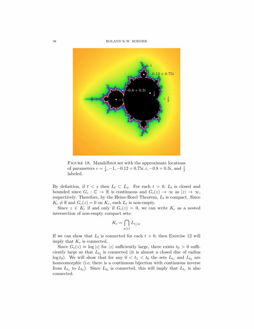
Figure 18. Mandelbrot set with the approximate locationsof parameters c = i

4 ,−1,−0.12 + 0.75i, i,−0.8 + 0.3i, and 12

labeled.

By definition, if t < s then Lt ⊂ Ls. For each t > 0, Lt is closed andbounded since Gc : C → R is continuous and Gc(z) → ∞ as |z| → ∞,respectively. Therefore, by the Heine-Borel Theorem, Lt is compact. SinceKc 6= ∅ and Gc(z) = 0 on Kc, each Lt is non-empty.

Since z ∈ Kc if and only if Gc(z) = 0, we can write Kc as a nestedintersection of non-empty compact sets:

Kc =⋂n≥1

L1/n.

If we can show that Lt is connected for each t > 0, then Exercise 12 willimply that Kc is connected.

Since Gc(z) ≈ log |z| for |z| sufficiently large, there exists t0 > 0 suffi-ciently large so that Lt0 is connected (it is almost a closed disc of radiuslog t0). We will show that for any 0 < t1 < t0 the sets Lt1 and Lt0 arehomeomorphic (i.e, there is a continuous bijection with continuous inversefrom Lt1 to Lt0). Since Lt0 is connected, this will imply that Lt1 is alsoconnected.


Mandelbrot set Julia Sets

Figure 19. Left: Zoomed-in view of the Mandelbrot setnear the cusp at c = 1

4 . Right: two filled Julia sets corre-sponding to points inside M and outside of M .

The following is a standard construction from Morse Theory; see [36,Theorem 3.1]. Because Gc is harmonic and has no critical points on A(∞),−∇Gc is a non-vanishing smooth vector field on A(∞). It is a relativelystandard smoothing construction to define a new vector field V : R2 → R2

that is smooth on all of C ≡ R2 and equals −∇Gc‖∇Gc‖2 for z ∈ C \ Lt1/2.

For any t ∈ [0,∞) let Φt : R2 → R2 denote the flow obtained by inte-grating V . According to the existence and uniqueness theorem for ordinarydifferential equations (see, e.g., [38]), Φt : R2 → R2 is a homeomorphismfor each t ∈ [0,∞). (We’re using that V “points inward” from ∞ so thatthe solutions exist for all time.)

For any z0 ∈ C \ Lt1/2 and any 0 ≤ t ≤ Gc(z0)− t1/2 we have

d

dtGc(Φt(z0)) = ∇Gc(Φt(z0)) · d

dtΦt(z0) = ∇Gc(Φt(z0)) · V (Φt(z0))

= ∇Gc(Φt(z0)) · −∇Gc(Φt(z0))

‖∇Gc(Φt(z0))‖2= −1.

In particular, Φt0−t1(Lt0) = Lt1 , implying that Lt0 is homeomorphic to Lt1 .


Now suppose that 0 has unbounded orbit under pc. In this case, 0 andall of its iterated preimages under pc are critical points of Gc. Since pchas a simple critical point at 0, one can check that these critical points ofGc are all “simple” in that the Hessian matrix of second derivatives hasnon-zero determinant. Moreover, by the Maximum Principle, they cannotbe local minima or local maxima. They are therefore saddle points. Fromthe property Gc(p(z)) = 2Gc(z), the saddle point at z = 0 is the one withthe largest value of Gc.

There are two paths along which we can start at 0 and walk uphill in thesteepest way possible—call them γ1 and γ2. Since 0 is the highest criticalpoint, they lead all the way from 0 out to ∞. Together with 0, these twopaths divide C into two domains U1 and U2. Meanwhile, there are twodirections that one can walk downhill from a saddle point. Walking thefastest way downhill leads to two paths η1 and η2 which lead to points inU1 and in U2 along which Gc(z) < Gc(0).

To make this idea rigorous, one considers the flow associated to the vectorfield −∇Gc. The saddle point 0 becomes a saddle type fixed point for theflow with the paths γ1 and γ2 being the stable manifold of this fixed point.The paths η1 and η2 are the unstable manifolds of this fixed point. (Seeagain [38].)

The union γ1 ∪ γ2 ∪ {0} divides the complex plane into two domains U1

and U2 with η1 ⊂ U1 and η2 ⊂ U2. We claim that both of these domainscontain points of Kc. Suppose for contradiction that one of them (sayU1) does not. Then, U1 ⊂ A(∞) and hence Gc would be harmonic onU1. However, Gc(z) ∼ log |z| for |z| large and Gc(z) > Gc(0) for pointsz ∈ γ1 ∪ γ2. Since Gc(z) < Gc(0) for points on η1, this would violate theMaximum Principle.

�

Remark. A stronger statement actually holds: if Kc is disconnected, thenit is a Cantor Set. (See [17] for the definition of Cantor Set.) In particular, itis totally disconnected: for any z, w ∈ Kc there exist open sets U, V ⊂ Csuch that Kc ⊂ U ∪ V , z ∈ U , w ∈ V , and U ∩ V = ∅. This follows fromthe fact that once Gc has the critical point 0 ∈ A(∞) then it actually hasinfinitely many critical points in A(∞). These additional critical points ofGc are the iterated preimages of 0 under pc.

For a somewhat different proof from the one presented above, includinga proof of this stronger statement, see [11, 12].

Exercise 29. Prove that if c 6= 0 then log |z2 + c| has a saddle-type criticalpoint at z = 0.


γ1

γ2

η10

η2

U1

U2

Figure 20. Stable and unstable trajectories of −∇Gc forthe critical point 0.

Hint: Write z = x+ iy and c = a+ bi and use that

log |z2 + c| = 1

2log(z2 + c

)(z2 + c

).

We will now state (without proofs) several interesting properties of theMandelbrot set:

Theorem. (Douady-Hubbard [14]) The Mandelbrot set M is connected.

(Nessim Sibony gave an alternate proof around the same time.) This theo-rem clears up the mystery about the black “dots” in Figure 16.

The following very challenging extended exercise leads the reader througha proof that M is connected that is related to the coloring of C\M accordingto the value of Gc(0). (It will be somewhat more convenient to considerGc(c) = Gc(pc(0)) = 2Gc(0).)

Extended Exercise 2. Let H : C→ R be given by H(c) = Gc(c). Provethat

(1) H is continuous,(2) H is harmonic on C \M ,(3) H is identically 0 on M ,(4) lim|c|→∞H(c) =∞, and(5) H has no critical points in C \M .

(Step 5 is the hardest part.) Use these facts to adapt the proof of the topo-logical characterization of the Mandelbrot Set to prove that M is connected.


Hausdorff Dimension extends the classical notion of dimension fromlines and planes to more general metric spaces. As the formal definition is abit complicated, we instead illustrate the notion with a few examples. A linehas Hausdorff dimension equal to 1 and the plane has Hausdorff dimensionequal to 2. A contour has Hausdorff dimension equal to 1 because, if youzoom in sufficiently far near any of the smooth points, the contour appearsmore and more like a straight line. However, sets of a “fractal nature” canhave non-integer Hausdorff Dimension. One example is the Koch Curve,which a simple closed curve in the plane that is obtained as the limit ofthe iterative process shown in Figure 21. No matter how far you zoom in,the Koch Curve looks the same as a larger copy of itself, and not like aline! This results in the Koch Curve having Hausdorff dimension equal tolog(4)/ log(3) ≈ 1.26. We refer the reader to [17] for a gentle introductionto Hausdorff Dimension.

Figure 21. The Koch Curve.

If S ⊂ C contains an open subset of C, then it is easy to see that it hasHausdorff Dimension equal to 2. It is much harder to imagine a subset of Cthat contains no such open set having Hausdorff Dimension 2. Therefore,the following theorem shows that the boundary ∂M of the Mandelbrot setM has amazing complexity. It also shows that for many parameters c from∂M the Julia set Jc has amazing complexity.

Theorem. (Shishikura [45]) The boundary of the Mandelbrot set ∂M hasHausdorff dimension equal to 2. Moreover, for a dense set of parametersc from the boundary of M the Julia set Jc has Hausdorff Dimension equalto 2.

Another interesting property of the Mandelbrot set is the appearance of“small copies” within itself. (Some of these were the “dots” from Figure 16.)Figure 22 shows a zoomed in view of M , where several small copies of M arevisible. These copies are explained by the renormalization theory [15, 34].

It would be remiss to not include one of the most famous conjecturesabout the Mandelbrot set. We first need


Figure 22. Zoomed-in view of part of the Mandelbrot setshowing two smaller copies. The approximate location wherewe have zoomed in is marked by the tip of the arrow in theinset figure.

Definition 22. A topological space X is locally connected if for everypoint x ∈ X and any open set V ⊂ X that contains x there is anotherconnected open set U with x ∈ U ⊂ V .

MLC Conjecture. The Mandelbrot set M is locally connected.

According to the Orsay Notes [13] of Douady and Hubbard, if this werethe case, then one could have a very nice combinatorial description of M .Given a proposed way that pc acts on the Julia set Jc (described by meansof the so called Hubbard Tree) one can use this combinatorial descriptionof M to find the desired value of c.

To better appreciate the difficulty in proving the MLC Conjecture, weinclude one more zoomed-in image of the Mandelbrot set in Figure 23.


Figure 23. Another zoomed-in view of part of the Mandel-brot set.

Let us finish the section, and our discussion of iterating quadratic poly-nomials, by returning to mathematics that can be done by undergraduates.The reader is now ready to answer Question 4 from Section 1.4:

Extended Exercise 3. Prove that for every m ≥ 1 there exists a pa-rameter c ∈ C such that pc(z) has an attracting periodic orbit of periodexactly m.

Hint: prove that there is a parameter c such that p◦mc (0) = 0 and p◦jc (0) 6= 0for each 0 ≤ j < m.

Lecture 4: “Complex dynamics and astrophysics.”

Most of the results discussed in Sections 1-3 of these notes are now quiteclassical. Let us finish our lectures with a beautiful and quite modernapplication of the Fatou-Julia Lemma to a problem in astrophysics [26, 24].We also mention that there are connections between complex dynamics andthe Ising model from statistical physics (see [7, 6] and the references therein)and the study of droplets in a Coulomb gas [30, 29].


4.1. Gravitational Lensing. Einstein’s Theory of General Relativity pre-dicts that if a point mass is placed directly between an observer and a lightsource, then the observer will see a ring of light, called an “Einstein Ring”.The Hubble Space Telescope has sufficient power to see these rings—onesuch image is shown in Figure 24. If the point mass is moved slightly, theobserver will see two different images of the same light source. With morecomplicated distributions of mass, like n point masses, the observer can seemore complicated images, resulting from a single point light source. Suchan image is shown in Figure 25. (Thanks to NASA for these images andtheir interpretations.)

There are many excellent surveys on gravitational lensing that are writ-ten for the mathematically inclined reader, including [25, 39, 48], as wellas the book [40]. We will be far more brief, with the goal of this lecturebeing to explain how Rhie [42] and Khavinson-Neumann [24] answered thequestion:

What is the maximum number of images that a single light source can havewhen lensed by n point masses?

We will tell some of the history of how this problem was solved and thenfocus on the role played by the Fatou-Julia Lemma.

Figure 24. An Einstein Ring. For more information, seehttp://apod.nasa.gov/apod/ap111221.html.

http://apod.nasa.gov/apod/ap111221.html


Figure 25. Five images of the same quasar(boxed) and three images of the same galaxy (cir-cled). The middle image of the quasar (boxed) isbehind the small galaxy that does the lensing. Formore information, see http://www.nasa.gov/multimedia/

imagegallery/image_feature_575.html

Suppose that n point masses lie on a plane that is nearly perpendicularto the line of sight between the observer and the light source and that theylie relatively close to the line of sight. If we describe their positions relativeto the line of sight to the light source by complex numbers zj and theirnormalized masses by σj > 0 for 1 ≤ j ≤ n, then the images of the lightsource seen by the observer are given by solutions z to the Lens Equation:

(20) z =

n∑j=1

σjz − zj

.

The “mysterious” appearance of complex conjugates on the right hand sideof this equation makes it difficult to study. It will be explained in Sec-tion 4.3, where we derive (20).

Exercise 30. Verify that (20) gives a full circle of solutions (Einstein Ring)when there is just one mass at z1 = 0. Then, verify that when z1 6= 0 thereare two solutions. Can you find a configuration of two masses so that (20)has five solutions?

http://www.nasa.gov/multimedia/imagegallery/image_feature_575.html

http://www.nasa.gov/multimedia/imagegallery/image_feature_575.html


Remark. Techniques from complex analysis extend nicely to lensing bymass distributions more complicated than finitely many points, includingelliptical [18] and spiral [4] galaxies.

The right hand side of (20) is of the form r(z), where r(z) is a rational

function r(z) = p(z)q(z) of degree n. (The degree of a rational function is

the maximum of the degrees of its numerator and denominator.) Thus, ourphysical question becomes the problem of bounding the number of solutionsto an equation of the form

z = r(z)(21)

in terms of n = deg(r(z)). Sadly, the Fundamental Theorem of Algebracannot be applied to

zq(z)− p(z) = 0(22)

because the resulting equation is a polynomial in both z and z. If onewrites z = x+ iy with x, y ∈ R, one can change (22) to a system of two realpolynomial equations

a(x, y) := Re(z q(z)− p(z)

)= 0 and

b(x, y) := Im(z q(z)− p(z)

)= 0,

each of which has degree n+ 1. So long as there are no curves of commonzeros for a(x, y) and b(x, y), Bezout’s Theorem (see, e.g., [27]) gives a boundon the number of solutions by (n+ 1)2.

In 1997, Mao, Petters, and Witt [35] exhibited configurations of n pointmasses at the vertices of a regular polygon in such a way that 3n+1 solutionswere found. They conjectured a linear bound for the number of solutionsto (20). For large n this would be significantly better than the bound givenby Bezout’s Theorem.

In 2003, Rhie [42] showed that if one takes the configuration of massesconsidered by Mao, Petters, and Witt and places a sufficiently small masscentered at the origin, then one finds 5n−5 solutions to (20). (We refer thereader also to [8, Section 5] for an another exposition on Rhie’s examples.)

In order to address a problem on harmonic mappings C → C posed byWilmshurst in [50], in 2003 Khavinson and Swiatek studied the number of

solutions to z = p(z) where p(z) is a complex polynomial. They proved

Theorem. (Khavinson-Swiatek [26]) Let p(z) be a complex polynomial

of degree n ≥ 2. Then, z = p(z) has at most 3n− 2 solutions.

Khavinson and Neumann later adapted the techniques from [26] to prove


Theorem. (Khavinson-Neumann [24]) Let r(z) be a rational function

of degree n ≥ 2. Then, z = r(z) has at most 5n− 5 solutions.

Apparently, Khavinson and Neumann solved this problem because of itsmathematical interest and only later were informed that they had actuallycompleted the solution to our main question of this lecture:

When lensed by n point masses, a single light source can have at most 5n−5images.

Remark. Geyer [20] used a powerful theorem of Thurston to show that

for every n ≥ 2 there is a polynomial p(z) for which z = p(z) has 3n − 2solutions, thus showing that Theorem 4.1 is sharp. It would be interestingto see an “elementary” proof.

4.2. Sketching the proof of the 5n−5 bound. We provide a brief sketchof the proof of the Khavinson-Neumann upper bound in the special casethat

r(z) =n∑j=1

σjz − zj

,(23)

with each σj > 0. It is the case arising in the Lens Equation (20). Thelocations {z1, . . . , zn} of the masses are called poles of r(z). They satisfylimz→zj |r(z)| =∞ for any 1 ≤ j ≤ n.

The function

f : C \ {z1, . . . , zn} → C given by f(z) = z − r(z)(24)

is an example of a harmonic mapping with poles since its real andimaginary parts are harmonic. It is orientation preserving near a pointz• with |r′(z•)| < 1 and orientation reversing (like a reflection z 7→ z)near points with |r′(z•)| > 1. A zero z• of f is simple if |r′(z•)| 6= 1 and asimple zero is called sense preserving if |r′(z•)| < 1 and sense-reversingif |r′(z•)| > 1.

Step 1: Reduction to Simple Zeros. Suppose r(z) is of the form (23)

and f(z) = z−r(z) has k zeros, some of which are not simple. Then, one canshow that there is an arbitrarily small perturbation of the locations of themasses so that the resulting rational function s(z) produces g(z) = z− s(z)having at least as many zeros as f(z) all of which are simple.

Therefore, it suffices to consider rational functions r(z) of the form (23)

such that each zero of f(z) = z − r(z) is simple.


Step 2: Argument Principle for Harmonic Mappings. Suffridge andThompson [49] adapted the Argument Principle to harmonic mappings withpoles f : C \ {z1, . . . , zk} → C.

Since r(z) has the form (23), limz→∞ |r(z)| = 0. Therefore, we can chooseR > 0 sufficiently large so that all of the poles of r(z) lie in D(0, R) andthe change of argument for f(z) while traversing γ = ∂D(0, R) counterclockwise is 1. This variant of the argument principle then gives

(m+ −m−) + n = 1(25)

where m+ is the number of sense preserving zeros, m− is the number ofsense reversing zeros, and n is the number of poles. (We are using that allof the zeros and poles are simple so that they do not need to be countedwith multiplicities.)

Step 3: Fatou-Julia Lemma Bound on m+: Zeros of f(z) correspondto fixed points for the anti-analytic mapping

z 7→ r(z).

Moreover, sense preserving zeros correspond to attracting fixed points (thosewith |r′(z•)| < 1).

Since the coefficients of r(z) are real, taking the second iterate yields

Q(z) = r(r(z)

)= r(r(z)),

which is an analytic rational mapping of degree n2. Such a mapping has2n2−2 critical points and an adaptation of the Fatou-Julia Lemma impliesthat each attracting fixed point of Q attracts a critical point.

However, the chain rule gives that critical points of Q(z) = r(r(z)) arethe critical points of r(z) and their inverse images under r(z). Since ageneric point has n inverse images under r, this can be used to show thateach attracting fixed point of Q(z) actually attracts n + 1 critical pointsof Q. Therefore, Q(z) has at most 2n− 2 attracting fixed points.

Since any sense preserving zero for f(z) is an attracting fixed point for Q,we conclude that m+ ≤ 2n− 2.

Step 4: Completing the proof: Since m+ ≤ 2n − 2, Equation (25)implies m− ≤ 3n− 3. Therefore, the total number of zeros is

m+ +m− ≤ 5n− 5.

The reader is encouraged to see [24] for the full details, including how toprove the bound for general rational functions r(z).


PL

S I

DLS

DL

DS

θ

β

O

α

α

PS

L ξ

Figure 26. S is the light source, I is an image, O is theobserver, L is a point mass, PL is the lens plane, PS is thesource plane.

4.3. Derivation of the Lens Equation. This derivation is a synthesisof ideas from [2] and [41, Section 3.1] that was written jointly with Ble-her, Homma, and Ji when preparing [8]. Since it was not included in thepublished version of [8], we present it here.

We will first derive the Lens Equation for one point mass using Figure 26,and then adapt it to N point masses. Suppose the observer is located atpoint O, the light source at a point S, and a mass M at point L. Also,suppose PL is the plane perpendicular to OL that contains L, and PS isthe plane perpendicular to OL that contains S. Due to the point mass, animage, I, will be created at angle α with respect to S.

Einstein derived using General Relativity that the bending angle is

α =4GM

c2ξ,(26)

where G is the universal gravitational constant and c is the speed of light,see [2].

The observer O describes the location S of the light source using anangle β and the perceived location I using another angle θ (see Figure 26).By a small angle approximation, ξ = DLθ, which we substitute into (26)


obtaining

α(θ) =4GM

c2DLθ.(27)

A small angle approximation also gives that DSI = DLSα(θ) = DSα(θ).Substituting this into β = θ − α(θ) gives

(28) β = θ − DLS

DSDL· 4GM

c2θ.

For β 6= 0, exactly two images are produced. When β = 0, the systemis rotationally symmetric about OL, thereby producing an Einstein Ring,whose angular radius is given by Equation (28).

In order to describe systems of two or more masses, we need to describelocations in the source plane PS and the lens plane PL using two-dimensionalvectors of angles (polar and azimuthal angles) as observed from O. Complexnumbers will be a good way to do this:

α = α(1) + iα(2), α = α(1) + iα(2), β = β(1) + iβ(2), and θ = θ(1) + iθ(2).

When there is only one mass, the whole configuration must still lie in oneplane, as in Figure 26. In particular, all four complex numbers have thesame argument, forcing us to replace the θ on the right hand side of (27)with θ:

α(θ) =4GM

c2DLθand hence β = θ − DLS

DSDL· 4GM

c2θ.(29)

This is why the complex conjugate arises in the Lens Equation (20).

We now generalize to n point masses. Let L be the center of mass ofthe n masses, and redefine SL as the plane that is perpendicular to OL andcontains L. We assume that the distance between L and the individual pointmasses is extremely small with respect to the pairwise distances betweenO, PL, and PS . Now consider the projection of the n point masses onto SL.We continue to let β ∈ C describe the location of the center of mass and

we describe the location of the jth point mass by εj = ε(1)j + iε

(2)j ∈ C. It

has mass Mj .In general, the bending angle is expressed as an integral expressed linearly

in terms of the mass distribution, see [41, Equation 3.57]. In particular, withpoint masses, the bending angle decomposes to a sum of bending angles,one for each point mass. Each is computed as in the one mass system:

αj =4GMj

c2DLθjwhere θj = θ − εj .


We obtain

β = θ −n∑j=1

αj = θ − DLS

DSDL

n∑j=1

4GMj

c2(θ − εj

) .Letting

w = β, z = θ, zj = εj , and σj =DLS

DSDL· 4GMj

c2

gives

(30) w = z −n∑j=1

σjz − zj

.

Equation (30) requires the assumption that the center of mass is the origin,i.e.

∑σjzj = 0. A translation by w allows us to fix the position of the

light source at the origin and vary the location of the center of mass. Thissimplifies Equation (30) to Equation (20).

4.4. Wilmshurst’s Conjecture. Let us finish our notes with an openproblem that can be explored by undergraduates. In [50], Wilmshurst con-sidered equations of the form

p(z) = q(z)(31)

where p(z) and q(z) are polynomials of degree n and m, respectively. Byconjugating the equation, if necessary, one may suppose n ≥ m. If m = n,then one can have infinitely many solutions (e.g. p(z) = zn = q(z)), butonce n > m Wilmshurst showed that there are finitely many solutions. Heconjectured that the number of solutions to (31) is at most 3n−2+m(m−1).

Unfortunately, this conjecture is false! Counterexamples were foundwhen m = n− 3 by Lee, Lerario, and Lundberg [28]. They propose:

Conjecture. (Lee, Lerario, Lundberg) If deg(p(z)) = n, deg(q(z)) = m,

and n > m, then the number of solutions to p(z) = q(z) is bounded by2m(n− 1) + n.

Note that this conjectured bound is not intended to be sharp. For example,Wilmshurst proved his conjecture in the case that m = n − 1, providing astronger bound in that case [50].

This problem was further studied using certified numerics by Hauenstein,Lerario, Lundberg, and Mehta [22]. Their work provides further evidencefor this conjecture.

Question. Can techniques from complex dynamics be used to prove thisconjecture?


References

[1] Lars V. Ahlfors. Complex analysis. McGraw-Hill Book Co., New York, third edition,1978. An introduction to the theory of analytic functions of one complex variable,International Series in Pure and Applied Mathematics.

[2] H. Asada. Perturbation theory of n point mass gravitational lens. Monthly Noticesof the Royal Astronomical Society, 394(2):818–830.

[3] Alan F. Beardon. Iteration of rational functions, volume 132 of Graduate Texts inMathematics. Springer-Verlag, New York, 1991. Complex analytic dynamical sys-tems.

[4] Steven R. Bell, Brett Ernst, Sean Fancher, Charles R. Keeton, Abi Komanduru, andErik Lundberg. Spiral galaxy lensing: a model with twist. Math. Phys. Anal. Geom.,17(3-4):305–322, 2014.

[5] Paul Blanchard. Complex analytic dynamics on the Riemann sphere. Bull. Amer.Math. Soc. (N.S.), 11(1):85–141, 1984.

[6] Pavel Bleher, Mikhail Lyubich, and Roland Roeder. Lee-Yang-Fisher zeros for DHLand 2D Rational Dynamics, II. Global Pluripotential Interpretation. Preprint availi-ble at: http://arxiv.org/abs/1107.5764.

[7] Pavel Bleher, Mikhail Lyubich, and Roland Roeder. Lee-Yang zeros for DHL and2D Rational Dynamics, I. Foliation of the Physical Cylinder. Preprint availible at:http://arxiv.org/abs/1009.4691.

[8] Pavel M. Bleher, Youkow Homma, Lyndon L. Ji, and Roland K. W. Roeder. Countingzeros of harmonic rational functions and its application to gravitational lensing. Int.Math. Res. Not. IMRN, (8):2245–2264, 2014.

[9] Boston University Java Applets for Dynamical Systems. http://math.bu.edu/

DYSYS/applets/

[10] Lennart Carleson and Theodore W. Gamelin. Complex dynamics. Universitext:Tracts in Mathematics. Springer-Verlag, New York, 1993.

[11] Robert L. Devaney. A first course in chaotic dynamical systems. Addison-WesleyStudies in Nonlinearity. Addison-Wesley Publishing Company, Advanced Book Pro-gram, Reading, MA, 1992. Theory and experiment, With a separately availablecomputer disk.

[12] Robert L. Devaney. An introduction to chaotic dynamical systems. Studies in Non-linearity. Westview Press, Boulder, CO, 2003. Reprint of the second (1989) edition.

[13] A. Douady and J. H. Hubbard. Etude dynamique des polynomes complexes. PartieI, volume 84 of Publications Mathematiques d’Orsay [Mathematical Publications ofOrsay]. Universite de Paris-Sud, Departement de Mathematiques, Orsay, 1984.

[14] Adrien Douady and John Hamal Hubbard. Iteration des polynomes quadratiquescomplexes. C. R. Acad. Sci. Paris Ser. I Math., 294(3):123–126, 1982.

[15] Adrien Douady and John Hamal Hubbard. On the dynamics of polynomial-like map-

pings. Ann. Sci. Ecole Norm. Sup. (4), 18(2):287–343, 1985.[16] Dynamics Explorer software. Written by Brian and Suzanne Boyd. http://

sourceforge.net/projects/detool/

[17] Gerald A. Edgar. Measure, topology, and fractal geometry. Undergraduate Texts inMathematics. Springer-Verlag, New York, 1990.

[18] C. D. Fassnacht, C. R. Keeton, and D. Khavinson. Gravitational lensing by ellipticalgalaxies, and the Schwarz function. In Analysis and mathematical physics, TrendsMath., pages 115–129. Birkhauser, Basel, 2009.

[19] Fractalstream dynamical systems software. Written by Matthew Noonan. https:

//code.google.com/p/fractalstream/downloads/list.

http://arxiv.org/abs/1107.5764


http://math.bu.edu/DYSYS/applets/

http://math.bu.edu/DYSYS/applets/

http://sourceforge.net/projects/detool/

http://sourceforge.net/projects/detool/

https://code.google.com/p/fractalstream/downloads/list

https://code.google.com/p/fractalstream/downloads/list


[20] Lukas Geyer. Sharp bounds for the valence of certain harmonic polynomials. Proc.Amer. Math. Soc., 136(2):549–555, 2008.

[21] Jacek Graczyk and Grzegorz Swiatek. Generic hyperbolicity in the logistic family.Ann. of Math. (2), 146(1):1–52, 1997.

[22] Jonathan Hauenstein, Antonio Lerario, Erik Lundberg, and Dhagash Mehta. Exper-iments on the zeros of harmonic polynomials using certified counting. To appear inExperimental Mathematics. See also http://arxiv.org/pdf/1406.5523.pdf.

[23] John Horgan. Mandelbrot set-to: Did the father of fractals “discover” his namesakeset? Scientific American, 262:30–34.

[24] Dmitry Khavinson and Genevra Neumann. On the number of zeros of certain rationalharmonic functions. Proc. Amer. Math. Soc., 134(4):1077–1085 (electronic), 2006.

[25] Dmitry Khavinson and Genevra Neumann. From the fundamental theorem of algebrato astrophysics: a “harmonious” path. Notices Amer. Math. Soc., 55(6):666–675,2008.

[26] Dmitry Khavinson and Grzegorz Swiatek. On the number of zeros of certain har-monic polynomials. Proc. Amer. Math. Soc., 131(2):409–414, 2003.

[27] Frances Kirwan. Complex algebraic curves, volume 23 of London Mathematical So-ciety Student Texts. Cambridge University Press, Cambridge, 1992.

[28] Seung-Yeop Lee, Antonio Lerario, and Lundberg Erik. Remarks on wilmshurst’stheorem. To appear in the Indiana University Math Journal. See also http://arxiv.

org/pdf/1308.6474.pdf.[29] Seung-Yeop Lee and Nikolai Makarov. Sharpness of connectivity bounds for quadra-

ture domains. Preprint: http://arxiv.org/abs/1411.3415.[30] Seung-Yeop Lee and Nikolai Makarov. Topology of quadrature domains. To appear

in the Journal of the AMS; see also http://arxiv.org/abs/1009.4691.[31] Mikhail Lyubich. Six Lectures on Real and Complex Dynamics (based on European

Lectures given in Barcelona, Copenhagen and St Petersburg in May-June 1999). Seehttp://www.math.sunysb.edu/~mlyubich/papers/lectures.ps.

[32] Mikhail Lyubich. Dynamics of rational transformations: topological picture. UspekhiMat. Nauk, 41(4(250)):35–95, 239, 1986.

[33] Mikhail Lyubich. Dynamics of quadratic polynomials. I, II. Acta Math., 178(2):185–247, 247–297, 1997.

[34] Mikhail Lyubich. Baby Mandelbrot sets, renormalization and MLC. Gaz. Math.,(113):45–50, 2007.

[35] S. Mao, A. O. Petters, and H. J. Witt. Properties of point mass lenses on a regularpolygon and the problem of maximum number of images. In The Eighth MarcelGrossmann Meeting, Part A, B (Jerusalem, 1997), pages 1494–1496. World Sci.Publ., River Edge, NJ, 1999.

[36] J. Milnor. Morse theory. Based on lecture notes by M. Spivak and R. Wells. Annalsof Mathematics Studies, No. 51. Princeton University Press, Princeton, N.J., 1963.

[37] John Milnor. Dynamics in one complex variable, volume 160 of Annals of Mathe-matics Studies. Princeton University Press, Princeton, NJ, third edition, 2006.

[38] Lawrence Perko. Differential equations and dynamical systems, volume 7. SpringerScience & Business Media, 2001.

[39] A. O. Petters. Gravity’s action on light. Notices Amer. Math. Soc., 57(11):1392–1409,2010.

[40] Arlie O. Petters, Harold Levine, and Joachim Wambsganss. Singularity theory andgravitational lensing, volume 21 of Progress in Mathematical Physics. BirkhauserBoston, Inc., Boston, MA, 2001. With a foreword by David Spergel.

http://arxiv.org/pdf/1406.5523.pdf





http://www.math.sunysb.edu/~mlyubich/papers/lectures.ps


[41] Arlie O. Petters, Harold Levine, and Joachim Wambsganss. Singularity theory andgravitational lensing, volume 21 of Progress in Mathematical Physics. BirkhauserBoston, Inc., Boston, MA, 2001. With a foreword by David Spergel.

[42] S. H. Rhie. n-point gravitational lenses with 5(n − 1) images. Preprint. arXiv:

astro-ph/0305166.[43] E.B. Saff and A.D. Snider. Fundamentals of Complex Analysis with Applications to

Engineering and Science, Third Edition. Prentice Hall, 2003.[44] Zhaiming Shen and Lasse Rempe-Gillen. The exponential map is chaotic: An invi-

tation to transcendental dynamics. To appear in American Mathematical Monthly.See also http://arxiv.org/pdf/1408.1129v2.pdf.

[45] Mitsuhiro Shishikura. The Hausdorff dimension of the boundary of the Mandelbrotset and Julia sets. Ann. of Math. (2), 147(2):225–267, 1998.

[46] Norbert Steinmetz. Rational iteration, volume 16 of de Gruyter Studies in Mathe-matics. Walter de Gruyter & Co., Berlin, 1993. Complex analytic dynamical systems.

[47] James Stewart. Calculus, 7th Edition. Cengage Learning, 2012.[48] Norbert Straumann. Complex Formulation of Lensing Theory and Applications. Hel-

vetica Physica Acta., 70(6):894-908, 1997.[49] T. J. Suffridge and J. W. Thompson. Local behavior of harmonic mappings. Complex

Variables Theory Appl., 41(1):63–80, 2000.[50] A. S. Wilmshurst. The valence of harmonic polynomials. Proc. Amer. Math. Soc.,

126(7):2077–2081, 1998.

arXiv:astro-ph/0305166

arXiv:astro-ph/0305166

http://arxiv.org/pdf/1408.1129v2.pdf

Index

analytic, 13–19, 26, 27, 31, 34, 48anti-analytic, 13, 48Argument Principle, 18, 48Attracting Periodic Orbit Lemma, 21,

22, 25, 27, 28, 30, 32

Bottcher’s Theorem, 22, 27Bezout’s Theorem, 46boundary, 11, 17, 18, 34, 41, 42

Cauchy Estimates, 17, 31, 34Cauchy Integral Formula, 16–18, 27Cauchy Integral Formula For Higher

Derivatives, 17, 19Cauchy’s Theorem, 15, 16, 19Cauchy-Riemann Equations, 13–15, 34closed disc, 11, 19, 31, 38compact, 12, 18, 19, 34, 37, 38complex polynomial, 2, 3, 13, 47conformal, 13, 22, 27connected, 11, 12, 22, 31, 32, 35, 38, 40,

42locally connected, 42

continuous, 12–14, 16, 34, 35, 37, 38contour, 11, 12, 14–19, 31, 41

closed, 11continuously deformed, 12positively oriented, 11simple, 11

critical point, 14, 30–32, 35–40, 48critical value, 14, 31

Density of Hyperbolicity Conjecture, 32differentiable, 13, 17, 19, 37disconnected, 11, 40domain, 11–14, 17–19, 34, 39

simply connected, 12, 14–17, 19, 31Douady, 1, 32, 35, 40, 42

Fatou-Julia Lemma, 30–32, 44, 48filled Julia set, 33, 35, 38fixed point, 7, 8, 20–23, 25–30, 33, 39,

48Fundamental Theorem of Algebra, 3, 45

Graczyk, 32Green function, 34, 35

harmonic function, 34

harmonic mapping, 47, 48Hauenstein, 52Hausdorff Dimension, 41Heine-Borel Theorem, 12, 38holomorphic, 13Hubbard, 1, 32, 40, 42

initial condition, 3–10, 20–22, 31Inverse Function Theorem, 13, 14, 27

Julia set, 34, 41–43

Kœnig’s Theorem, 22Khavinson, 44, 47

Lee, 51Lens Equation, 44, 47, 49, 50Lerario, 51Lundberg, 51Lyubich, 1, 32

Mandelbrot set, 20, 30, 32, 33, 35–38,40–43

Maximum Modulus Principle, 18–20Maximum Principle, 34, 39Mehta, 52MLC Conjecture, 42

neighborhood, 11, 13, 14, 22, 23, 27Neumann, 44, 47

orbit, 4–10, 20–22, 25, 30Orsay Notes, 1, 42

parameter, 4, 6, 10, 22, 27–29, 32, 34,35, 37, 41–43

periodic orbit, 20attracting, 10, 20–22, 24, 25, 27–33,

35, 43, 48basin of attraction, 22immediate basin, 22multiplier, 21, 22, 25, 27–30

periodic points, 20, 28

Rhie, 44, 46

Swiatek, 32, 47Schwarz Lemma, 19, 21shift of coordinates, 21, 25, 30Shishikura, 42

56


Simply-Connected Inverse FunctionTheorem, 14, 31

Topological Characterization of theMandelbrot Set, 35

Uniform Limits of Harmonic Functions,34, 37

Uniform Limits Theorem, 18, 19, 26

Wilmshurst’s Conjecture, 51

AROUND THE BOUNDARY OF COMPLEX DYNAMICS.

Documents

Transcript of AROUND THE BOUNDARY OF COMPLEX DYNAMICS.