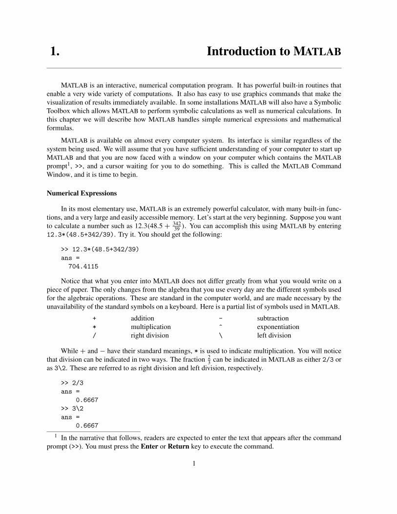
1. Introduction to MATLAB

MATLAB is an interactive, numerical computation program. It has powerful built-in routines thatenable a very wide variety of computations. It also has easy to use graphics commands that make thevisualization of results immediately available. In some installations MATLAB will also have a SymbolicToolbox which allows MATLAB to perform symbolic calculations as well as numerical calculations. Inthis chapter we will describe how MATLAB handles simple numerical expressions and mathematicalformulas.

MATLAB is available on almost every computer system. Its interface is similar regardless of thesystem being used. We will assume that you have sufficient understanding of your computer to start upMATLAB and that you are now faced with a window on your computer which contains the MATLABprompt1, >>, and a cursor waiting for you to do something. This is called the MATLAB CommandWindow, and it is time to begin.

Numerical Expressions

In its most elementary use, MATLAB is an extremely powerful calculator, with many built-in func-tions, and a very large and easily accessible memory. Let’s start at the very beginning. Suppose you wantto calculate a number such as 12.3(48.5 + 342

39 ). You can accomplish this using MATLAB by entering12.3*(48.5+342/39). Try it. You should get the following:

>> 12.3*(48.5+342/39)ans =704.4115

Notice that what you enter into MATLAB does not differ greatly from what you would write on apiece of paper. The only changes from the algebra that you use every day are the different symbols usedfor the algebraic operations. These are standard in the computer world, and are made necessary by theunavailability of the standard symbols on a keyboard. Here is a partial list of symbols used in MATLAB.

+ addition - subtraction* multiplication ^ exponentiation/ right division \ left division

While + and − have their standard meanings, * is used to indicate multiplication. You will noticethat division can be indicated in two ways. The fraction 2

3 can be indicated in MATLAB as either 2/3 oras 3\2. These are referred to as right division and left division, respectively.

>> 2/3ans =

0.6667>> 3\2ans =

0.6667

1 In the narrative that follows, readers are expected to enter the text that appears after the commandprompt (>>). You must press the Enter or Return key to execute the command.

1

Exponentiation is quite different in MATLAB; it has to be, since MATLAB has no way of enteringsuperscripts. Consequently, the power 43 must be entered as 4^3.

>> 4^3ans =

64

The order in which MATLAB performs arithmetic operations is exactly that taught in high schoolalgebra courses. Exponentiations are done first, followed by multiplications and divisions, and finally byadditions and subtractions. The standard order of precedence of arithmetic operations can be changedby inserting parentheses. For example, the result of 12.3*(48.5+342)/39 is quite different than thesimilar expression we computed earlier, as you will discover if you try it.

MATLAB allows the assignment of numerical values to variable names. For example, if you enter

>> x = 3x =

3

then MATLAB will remember that x stands for 3 in subsequent computations. Therefore, computing2.5*x will result in

>> 2.5*xans =

7.5000

You can also assign names to the results of computations. For example,

>> y = (x+2)^3y =

125

will result in y being given the value (3 + 2)3 = 125.

You will have noticed that if you do not assign a name for a computation, MATLAB will assign thedefault name ans to the result. This name can always be used to refer to the results of the previouscomputation. For example:

>> 2+3ans =

5

>> ans/5ans =

1

MATLAB has a few preassigned variables or constants. The constant π = 3.14159... is given thename pi.

>> pians =

3.1416

2

The square root of −1 is i.

>> sqrt(-1)ans =

0 + 1.0000i

Engineers and physicists frequently use i to represent current, so they prefer to use j for the square rootof −1. MATLAB is well aware of this preference.

>> jans =

0 + 1.0000i

There is no symbol for e, the base of the natural logarithms, but this can be easily computed as exp(1).

>> exp(1)ans =

2.7183

Mathematical Functions

There is a long list of mathematical functions that are built into MATLAB. Included are all of thefunctions that are standard in calculus courses.

Elementary Functions

abs(x) The absolute value of x, i.e. |x|.sqrt(x) The square root of x, i.e.

√x.

sign(x) The signum of x, i.e. 0 if x = 0, −1 if x < 0, and +1 if x > 0.

The Trigonometric Functions

sin(x) The sine of x, i.e. sin(x).cos(x) The cosine of x, i.e. cos(x).tan(x) The tangent of x, i.e. tan(x).cot(x) The cotangent of x, i.e. cot(x).sec(x) The secant of x, i.e. sec(x).csc(x) The cosecant of x, i.e. csc(x).

The Inverse Trigonometric Functions

asin(x) The inverse sine of x, i.e. arcsin(x) or sin−1(x).acos(x) The inverse cosine of x, i.e. arccos(x) or cos−1(x).atan(x) The inverse tangent of x, i.e. arctan(x) or tan−1(x).acot(x) The inverse cotangent of x, i.e. arccot(x) or cot−1(x).asec(x) The inverse secant of x, i.e. arcsec(x) or sec−1(x).acsc(x) The inverse cosecant of x, i.e. arccsc(x) or csc−1(x).

3

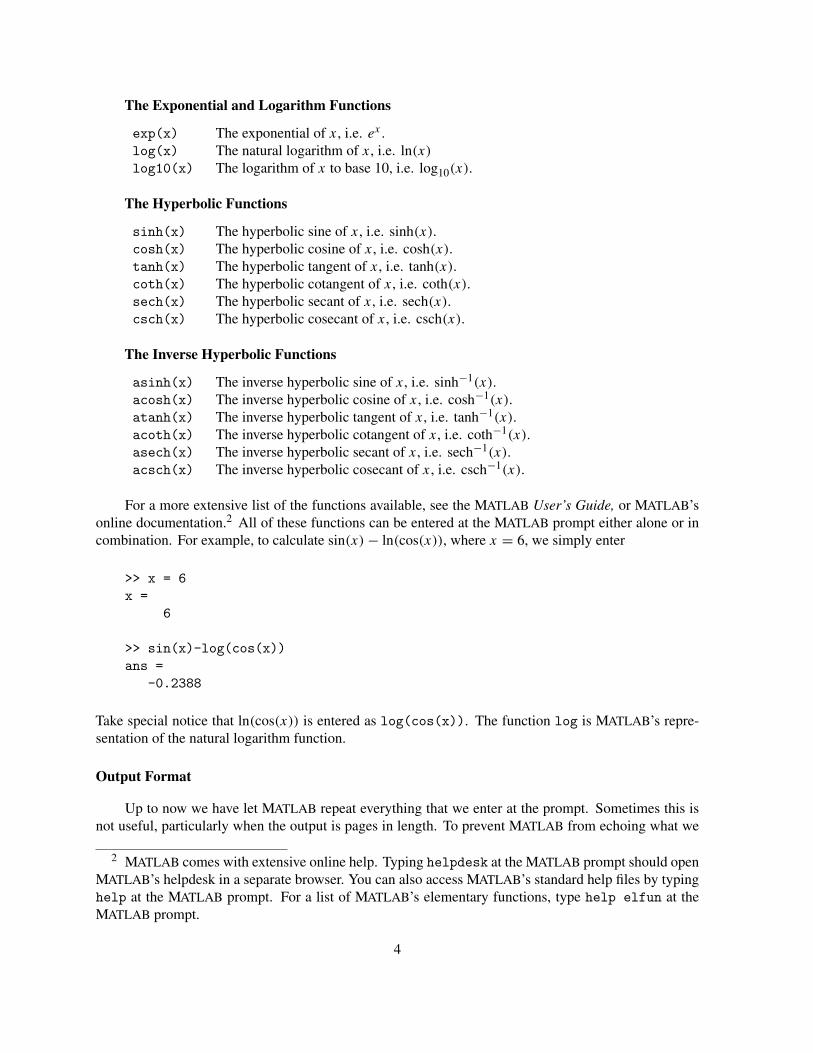
The Exponential and Logarithm Functions

exp(x) The exponential of x, i.e. ex .log(x) The natural logarithm of x, i.e. ln(x)

log10(x) The logarithm of x to base 10, i.e. log10(x).

The Hyperbolic Functions

sinh(x) The hyperbolic sine of x, i.e. sinh(x).cosh(x) The hyperbolic cosine of x, i.e. cosh(x).tanh(x) The hyperbolic tangent of x, i.e. tanh(x).coth(x) The hyperbolic cotangent of x, i.e. coth(x).sech(x) The hyperbolic secant of x, i.e. sech(x).csch(x) The hyperbolic cosecant of x, i.e. csch(x).

The Inverse Hyperbolic Functions

asinh(x) The inverse hyperbolic sine of x, i.e. sinh−1(x).acosh(x) The inverse hyperbolic cosine of x, i.e. cosh−1(x).atanh(x) The inverse hyperbolic tangent of x, i.e. tanh−1(x).acoth(x) The inverse hyperbolic cotangent of x, i.e. coth−1(x).asech(x) The inverse hyperbolic secant of x, i.e. sech−1(x).acsch(x) The inverse hyperbolic cosecant of x, i.e. csch−1(x).

For a more extensive list of the functions available, see the MATLAB User’s Guide, or MATLAB’sonline documentation.2 All of these functions can be entered at the MATLAB prompt either alone or incombination. For example, to calculate sin(x) − ln(cos(x)), where x = 6, we simply enter

>> x = 6x =

6

>> sin(x)-log(cos(x))ans =

-0.2388

Take special notice that ln(cos(x)) is entered as log(cos(x)). The function log is MATLAB’s repre-sentation of the natural logarithm function.

Output Format

Up to now we have let MATLAB repeat everything that we enter at the prompt. Sometimes this isnot useful, particularly when the output is pages in length. To prevent MATLAB from echoing what we

2 MATLAB comes with extensive online help. Typing helpdesk at the MATLAB prompt should openMATLAB’s helpdesk in a separate browser. You can also access MATLAB’s standard help files by typinghelp at the MATLAB prompt. For a list of MATLAB’s elementary functions, type help elfun at theMATLAB prompt.

4

tell it, simply enter a semicolon at the end of a command. For example, enter

>> q=7;

and then ask MATLAB what it thinks q is by entering

>> qq =

7

If you use MATLAB to compute cos(π), you get

>> cos(pi)ans =

-1

In this case MATLAB is smart enough to realize that the answer is an integer and it displays the answerin that form. However, cos(3) is not an integer, and MATLAB gives us -0.9900 as its value. Thus, ifMATLAB is not sure that a number is an integer, it displays five significant figures in its answer. Asanother example, 1.57 is very close to π/2, and cos(π/2) = 0. MATLAB gives us

>> cos(1.57)ans =

7.9633e-004

This is an example of MATLAB’s exponential, or scientific notation. It stands for 7.9633 × 10−4, or0.00079633. In this case MATLAB again displays five significant digits in its answer. All of theseillustrate the default format, which is called the short format. It is important to realize that althoughMATLAB only displays five significant digits in the default format, it is computing the answer to anaccuracy of sixteen significant figures.

There are several other formats. We will discuss two of them. If it is necessary or desirable tohave more significant digits displayed, enter format long at the MATLAB prompt. MATLAB will thendisplay about sixteen significant digits. For example,

>> format long>> cos(1.57)ans =

7.963267107332634e-004

There is another output format which we will find useful. If you enter format rat, then all numberswill be shown as rational numbers. This is called the rational format. If the numbers are actually irrational,MATLAB will find a very close rational approximation to the number.

>> cos(1.57)ans =

47/59021

The rational format is most useful when you are working with numbers you know to be rational. Afterusing a different format, you can return to the standard, short format by entering format short.

5

Complex Arithmetic

One of the nicest features of MATLAB is that it works as easily with complex numbers as it doeswith real numbers. The complex number z = 2 − 3i is entered exactly as it is written.

>> z = 2-3iz =

2.0000 - 3.0000i

Then if we enter w = 3 + 5i, we can calculate sums, products, and quotients of these numbers in exactlythe same way we do for real numbers. For example,

>> w = 3+5i;>> z*wans =21.0000 + 1.0000i

and

>> z/wans =-0.2647 - 0.5588i

Any of the arithmetic functions listed earlier can be applied to complex numbers. For example,

>> y = sqrt(w)y =

2.1013 + 1.1897i

and

>> y*yans =

3.0000 + 5.0000i

Since y2 = w, it is a square root of the complex number w. The reader might try cos(w) and exp(w).In particular, the reader might wish to verify Euler’s formula

eiθ = cos(θ) + i sin(θ)

for several values of θ , including θ = 2π, π, π/2.

>> theta = pi; exp(i*theta), cos(theta) + i*sin(theta)ans =-1.0000 + 0.0000i

ans =-1.0000 + 0.0000i

6

Note that several MATLAB commands can be placed on a single line, separated by commas, or semicolons,should you desire to suppress the output.

The ease with which MATLAB handles complex numbers has one drawback. There is at least onecase where the answer is not the one we expect. Use MATLAB to calculate (−1)1/3. Most people wouldexpect the answer −1, but MATLAB gives us

>> (-1)^(1/3)ans =

0.5000 + 0.8660i

At first glance this may seem strange, but if you cube this complex number you do get −1. ConsequentlyMATLAB is finding a complex cube root of −1, while we would expect a real root. The situation is evenworse, since in most of the cases where this will arise in this manual, it is not the complex cube root wewant. We will want the cube root of −1 to be −1.

However, this is a price we have to pay for other benefits. For MATLAB to be so flexible that it cancalculate roots of arbitrary order of arbitrary complex numbers, it is necessary that it should give whatseems like a strange answer for the cube root of negative numbers. In fact the same applies to any oddroot of negative numbers. What we need is a way to work around the problem.

Notice that if x < 0, then x = −1 × |x|, and we can find a negative cube root as −1 × |x|1/3.Here we are taking the real cube root of the positive number |x|, and MATLAB does that the way wewant it done. But suppose the situation arises where we do not know beforehand whether x is positiveor negative. What we want is

x1/3 =⎧

⎨

⎩

|x|1/3, if x > 0;0, if x = 0;−1 × |x|1/3, if x < 0.

To write this more succinctly we use the signum function sgn(x) (in MATLAB it is denoted by sign(x)).This function is defined to be

sgn(x) ={ 1, if x > 0;

0, if x = 0;−1, if x < 0.

Thus, in all cases we have x = sgn(x) |x|, and the real cube root is

x1/3 = sgn(x) |x|1/3.

In MATLAB, we would enter sign(x)*abs(x)^(1/3).

Recording Your Work

It is frequently useful to be able to record what happens in a MATLAB session. For example, in theprocess of preparing a homework submission, it should not be necessary to copy all of the output from thecomputer screen. You ought to be able to do this automatically. The MATLAB diary command makesthis possible.

For example, suppose you are doing your first homework assignment and you want to record whatyou are doing in MATLAB. To do this, choose a name, perhaps hw1, for the file in which you wish torecord the output. Then enter diary hw1 at the MATLAB prompt. From this point on, everything that

7

appears in the Command Window will also be recorded in the file hw1. When you want to stop recordingenter diary off. If you want to start recording again, enter diary on.

The file that is created is a simple text file. It can be opened by an editor or a word processingprogram and edited to remove extraneous material, or to add your comments. You can use the MATLABeditor for this process. To access it, first be sure you have stopped the editing process by executing diaryoff. Next, either click on the open file in the Toolbar, or select Open file from the Edit menu. The fileselection window that opens is set to display only MATLAB files, so the text diary file will not be visible.Click on the Files of type: popup menu and select All Files. Then select the name of your diary file. Youwill now be able to make any changes you want in the file. You will also be able to print the file to get ahard copy.

To open your diary file, or any other file you create with MATLAB, you will have to know where itis stored on your computer. This means that you will have to understand the directory structure on yourcomputer. (We are using directory as a synonym of file folder.) Your diary file is saved in the currentdirectory. In MATLAB 6, the current directory is displayed in a small box at the top of the commandwindow. Next to it there is a button with three dots (an ellipsis) on it. Clicking this button will opena new window containing the directory tree of your computer. You can make any directory the currentdirectory by selecting it from the directory tree.

Different operating systems provide different ways of handling files and directories. However, it ispossible to do a lot of file handling entirely within MATLAB. For this purpose MATLAB uses a combinationof UNIX and DOS commands. You can find the name of the current directory by using the command pwd.The response will be the full address of the current directory in the language of your operating system.You can obtain a list of the files in the current directory with the commands ls or dir. You can changedirectories with the commands cd or chdir. You can make a new directory with the command mkdir.We suggest that you use the help command3 to find out more, and experiment with these commands tolearn what they do in your system.

Exercises

1. Use the standard procedure on your computer system to create a folder named mywork. In MATLAB changeto this folder either by using the command cd at the MATLAB prompt or by clicking the ellipsis (. . . )button next to the Current Directory edit box on your MATLAB toolbar and browsing to the folder mywork.Look at the Current Directory edit box to be sure that mywork is the current directory. You can also use thecommand pwd at the MATLAB prompt. Clear the command window with the command clc, then clear yourworkspace of all variables with the command clear. Start a diary session with diary hmwk1. Read Chapter1 (Introduction to Matlab) of this manual again, but this time enter each of the commands in the narrativeat the MATLAB prompt as you read. When you are finished, enter the command diary off. Open the filehmwk1 in your favorite editor or word processor (or open it in Matlab’s editor by typing edit hmwk1 at theMATLAB prompt). Edit and correct any mistakes that you made. Save and print the edited file and submitthe result to your instructor.

3 For example, type help cd to obtain help on using the command cd.

8

2. Plotting in MATLAB

MATLAB provides several methods for plotting the graphs of functions and more general curves.The easiest to use is what we will call EZ plotting, since it uses the command ezplot and its variants.While it is easy to use it lacks flexibility. We will briefly explain EZ plotting in the first section. Thesecond method we will describe uses the commands plot and plot3. It provides more flexibility atthe cost of some ease of use. It is the principal method used in this manual, so we will explain it insome detail. At the end of this chapter we will introduce MATLAB’s handle graphics. The use of handlegraphics gives the user complete control over the graphic, but it is not so easily used.

EZ plotting

To plot the sine function in MATLAB, simply execute the command

>> ezplot('sin(x)')

The result is shown in Figure 2.1. You will notice that ezplot produces the plot of sin(x) over the interval[−2π, 2π ]. Next execute

>> ezplot('x*exp(-x^2)')

This time the plot, shown in Figure 2.2, is over an interval slightly bigger than [−2.5, 2.5].

−6 −4 −2 0 2 4 6

−1

−0.5

0

0.5

1

x

sin(x)

−2.5 −2 −1.5 −1 −0.5 0 0.5 1 1.5 2 2.5−0.5

−0.4

−0.3

−0.2

−0.1

0

0.1

0.2

0.3

0.4

0.5

x

x exp(−x2)

Figure 2.1. Plot of sin x. Figure 2.2. Plot of xe−x2.

Notice that you did not have to specify a plot interval. The command ezplot uses [−2π, 2π ] asthe default interval over which to produce a plot. If the function is almost constant near the endpoints of

9

the interval [−2π, 2π ], as is xe−x2, then ezplot chooses a smaller interval. If the default interval does

not please you, you can choose your own. For example, execute

>> ezplot('sin(x)',[0,8*pi])

to plot the sine function over the interval [0, 8π ].

Example 1. The initial value problem y′ = y + t with y(0) = 0 has the solution y(t) = et − t − 1. Plotthis solution over the interval 0 ≤ t ≤ 2.

This can be done with the single command ezplot('exp(t)-t-1',[0,2]).

The command ezplot can also plot curves that are defined implicitly or parametrically. To learnabout these features execute help ezplot. This command also illustrates the use of the command help.Whenever you run across a command you do not understand, use the help command. It will provideyou with the information you need.

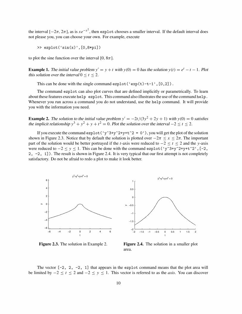
Example 2. The solution to the initial value problem y′ = −2t/(3y2 + 2y + 1) with y(0) = 0 satisfiesthe implicit relationship y3 + y2 + y + t2 = 0. Plot the solution over the interval −2 ≤ t ≤ 2.

If you execute the command ezplot('y^3+y^2+y+t^2 = 0'), you will get the plot of the solutionshown in Figure 2.3. Notice that by default the solution is plotted over −2π ≤ x ≤ 2π. The importantpart of the solution would be better portrayed if the t-axis were reduced to −2 ≤ t ≤ 2 and the y-axiswere reduced to −2 ≤ y ≤ 1. This can be done with the command ezplot('y^3+y^2+y+t^2',[-2,2, -2, 1]). The result is shown in Figure 2.4. It is very typical that our first attempt is not completelysatisfactory. Do not be afraid to redo a plot to make it look better.

−6 −4 −2 0 2 4 6

−6

−4

−2

0

2

4

6

t

y

y3+y2+y+t2 = 0

−2 −1.5 −1 −0.5 0 0.5 1 1.5 2−2

−1.5

−1

−0.5

0

0.5

1

t

y

y3+y2+y+t2 = 0

Figure 2.3. The solution in Example 2. Figure 2.4. The solution in a smaller plotarea.

The vector [-2, 2, -2, 1] that appears in the ezplot command means that the plot area willbe limited by −2 ≤ t ≤ 2 and −2 ≤ y ≤ 1. This vector is referred to as the axis. You can discover

10

the axis of the current plot by executing axis on the command line. Execute help axis to learn moreabout this versatile command. For example, the same reduction of plot area can be accomplished withthe command axis([-2, 2, -2, 1]) after the plot in Figure 2.3 was done.

If you own the Symbolic Toolbox, an add-on product to MATLAB, the command ezplot providesan excellent way to get a quick plot of the solution of an initial value problem.

Example 3. Graph the solution of y′ − y = e−t cos 3t, with y(0) = 1.

Enter the command

>> dsolve('Dy - y = exp(-t)*cos(3*t)','y(0) = 1')ans =-2/13*exp(-t)*cos(3*t)+3/13*sin(3*t)*exp(-t)+15/13*exp(t)

Then the command

>> ezplot(ans)

will provide a plot of the solution. We discuss the Symbolic Toolbox in Chapter 10.

Matrices and Vectors in MATLAB

To use the plot command effectively it is necessary to know a little about how MATLAB works.A powerful feature of MATLAB is that every numerical quantity is considered to be a complex matrix!1

For those of you who do not already know, a matrix is a rectangular array of numbers. For example,

A =[

1 π√−1√

2 4 0

]

is a matrix with 2 rows and 3 columns.

If you want to enter the matrix A into MATLAB proceed as follows:

>> A = [1,pi,sqrt(-1);sqrt(2),4,0]A =

1.0000 3.1416 0 + 1.0000i1.4142 4.0000 0

Note that commas are used to separate the individual elements in a row, and semicolons are used toseparate the rows of the matrix. You can also use spaces to separate (delimit) the entries in a row. Thus,the command A = [1 pi sqrt(-1);sqrt(2) 4 0] can be used to enter A into MATLAB.

The size of a matrix is the number of rows and columns. For example,

>> size(A)ans =

2 3

1 A matrix whose entries are complex numbers.

11

verifies that A has 2 rows and 3 columns. Two matrices are said to have the same size if they have thesame number of rows and the same number of columns.

Even single numbers in MATLAB are matrices. For example,

>> a = 5;>> size(a)ans =

1 1

shows that MATLAB thinks that 5, or any other complex number, is a matrix with one row and one column.

A vector is a list of numbers.2 It can be a vertical list, in which case it is called a column vector, orit can be a horizontal list, in which case it is called a row vector. Vectors are special cases of matrices, soyou can enter the row vector v = [1, −5, π,

√−1] into MATLAB using the command

v = [1,-5,pi,sqrt(-1)]

or v = [1 -5 pi sqrt(-1)]. On the other hand, we can define a column vector with the command u =[1;2;3;4]. It is important to remember that MATLAB distinquishes between row and column vectors.

In MATLAB, the length of a vector is the number of elements in the list. For example, the MATLABlength of each of the vectors u and v defined in the previous paragraph is 4. The MATLAB commandlength will disclose the length of any vector. Try length(u) and length(v). Notice that u and v havethe same length, but not the same size, since u is a column vector and v is a row vector.

This notion of length is not to be confused with the geometric length of a vector, defined to be thesquare root of the sum of the squares of the absolute values of the entries. MATLAB’s command forfinding the geometric length of a vector is norm. For example,

>> norm(v)ans =

6.0720

Addition, Subtraction, and Multiplication by Scalars

If A and B are matrices of the same size, then they can be added together. For example,

2 The word vector is one of the most over used terms in mathematics and its applications. To aphysicist or a geometer, a vector is a directed line segment. To an algebraist or to many engineers, avector is a list of numbers. To users of more advanced parts of linear algebra, a vector is an element of avector space. In this latter, most general case, a vector could be any of the above examples, a polynomial,a more general function, or an example of, quite literally, any class of mathematical objects which canbe added together and scaled by multiplication.

All too often the meaning in any particular situation is not explained. The result is very confusingto the student. When the word vector appears, a student should make a concerted effort to discover themeaning that is used in the current setting.

When using MATLAB, the situation is clear. A vector is a list of numbers, which may be complex.

12

>> A = [1 2;3 4], B = [5,6;7,8], C = A + BA =

1 23 4

B =5 67 8

C =6 8

10 12

You will notice that each element of the matrix C is sum of the corresponding elements in the matrices A

and B. The same is true for the difference of two matrices. Try C-A, and see what you get (you shouldget B).

You can multiply or divide any matrix by a scalar.

>> v = ones(1,5); w = 4*v, z = v/2w =

4 4 4 4 4z =

0.5000 0.5000 0.5000 0.5000 0.5000

While multiplication and division by scalars are standard parts of matrix algebra, the addition of ascalar to, or the subtraction of a scalar from a matrix are not standard algebra. However, they are allowedin MATLAB. Try

>> m = v - 3, a = v + 4m =

-2 -2 -2 -2 -2a =

5 5 5 5 5

MATLAB’s transpose operator (a single apostrophe) changes a column vector into a row vector (andvice-versa).

>> u = [1;2], v = u'u =

12

v =1 2

Actually, .' is MATLAB’s transpose operator and ' is MATLAB’s conjugate transpose operator. Enter A= [1+i,-2;3i,2-i], then type A' and view the results. Note that rows of A have become columns, buteach entry has been replaced with its complex conjugate. Type A.' to appreciate the difference. If eachentry of a matrix is a real number, then it doesn’t matter whether you use ' or .'.

13

Array Operations and Array Smart Functions

MATLAB has built-in, element-by-element, operations for other mathematical operations on matricesFor example, should you need to multiply two vectors on an element-by-element basis, use MATLAB’s.* operator.

>> v = [1,2,3,4], w = [5,6,7,8], u = v.*wv =

1 2 3 4w =

5 6 7 8u =

5 12 21 32

If you look closely, you will see that u is a vector of the same size as v and w, and that each element in u isthe product of the corresponding elements in v and w. This operation is called array multiplication, andMATLAB’s symbol for it is .*, not *. MATLAB uses * for matrix multiplication, which is quite differentfrom array multiplication. Try entering v*w and see what happens. We will explain matrix multiplicationin Chapter 11.

There are other array operations. All of them act element-by-element. Try v./w and w./v. Thisis array right division. Then try v.\w and w.\v, and compare the results. This is called array leftdivision. There is one other array operation — array exponentiation. This is also an element-by-elementoperation. The operation A.^2 results in every element of the matrix A being raised to the second power.For example, if A = [1,2;3,4], the command

>> A = [1,2;3,4], B = A.^2A =

1 23 4

B =1 49 16

raises each entry in A to the second power. The command A^2 is equivalent to A*A, which gives an entirelydifferent result. Try it and see. For all array operations it is required that the matrices have exactly thesame size. You might try [1,2;3,4].*[1;1] to see what happens when they are not.

The built-in MATLAB functions, which we discussed briefly in Chapter 1, are all designed to bearray smart. This means that if you apply them to a matrix, the result will be the matrix obtained byapplying the function to each individual element. For example:

>> theta = [0,pi/2,pi,3*pi/2,2*pi], y = cos(theta)theta =

0 1.5708 3.1416 4.7124 6.2832y =

1.0000 0.0000 -1.0000 0.0000 1.0000

This is an extremely important feature of MATLAB, as you will discover in the next section.

14

Plotting in MATLAB Using the plot Command

None of these array operations would be important if it were not so easy to create and use vectorsand matrices in MATLAB. Here is a typical situation. Suppose we want to define a vector that containsa large number of equally spaced points in an interval [a, b]. MATLAB’s start:increment:finishconstruct allows you to generate equally spaced points with ease. For example, the command

>> t = 0:0.2:1t =

0 0.2000 0.4000 0.6000 0.8000 1.0000

generates numbers from 0 to 1 in increments of 0.2.3 The command y = t.^3 will produce a vector ywith 6 entries, each the cube of the corresponding entry in the vector t.

>> y = t.^3y =

0 0.0080 0.0640 0.2160 0.5120 1.0000

We can get a rudimentary plot of the function y = t3 by plotting the entries of y versus the entriesof t. MATLAB will do this for us. The command

>> plot(t,y)

will produce a plot of y versus t in the current figure window. If no figure window exists, then thecommand plot will create one for you. MATLAB plots the 6 ordered pairs (t, y) generated by the vectorst and y, connecting consecutive ordered pairs with line segments, to produce an plot similar to the thatshown in Figure 2.5.

0 0.1 0.2 0.3 0.4 0.5 0.6 0.7 0.8 0.9 10

0.1

0.2

0.3

0.4

0.5

0.6

0.7

0.8

0.9

1

0 0.1 0.2 0.3 0.4 0.5 0.6 0.7 0.8 0.9 10

0.1

0.2

0.3

0.4

0.5

0.6

0.7

0.8

0.9

1

Figure 2.5. A simple plot Figure 2.6. A simple plot with refined data.

3 If you omit theincrement, as in t = 0:10, MATLAB automatically increments by 1. For example,try q = 0:10.

15

Notice that the plot in Figure 2.5 is kinky. This is because we plotted too few points before MATLABconnected the dots with straight lines. If we use enough points we get a smooth looking curve. Forexample, the commands

>> t = 0:0.05:1; y = t.^3; plot(t,y), shg

produced the graph in Figure 2.6. This time there are 21 points, and the curve appears smooth. Notice thatmultiple commands can be entered on a single command line if they are separated with commas and/orsemicolons. The command shg stands for “show the graph,” and it brings the current figure window 4 tothe front. It is a good idea to add shg to plot commands on the command window.

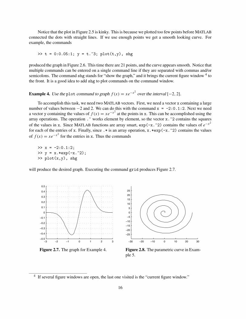
Example 4. Use the plot command to graph f (x) = xe−x2over the interval [−2, 2].

To accomplish this task, we need two MATLAB vectors. First, we need a vector x containing a largenumber of values between −2 and 2. We can do this with the command x = -2:0.1:2. Next we needa vector y containing the values of f (x) = xe−x2

at the points in x. This can be accomplished using thearray operations. The operation .^ works element by element, so the vector x.^2 contains the squaresof the values in x. Since MATLAB functions are array smart, exp(-x.^2) contains the values of e−x2

for each of the entries of x. Finally, since .* is an array operation, x.*exp(-x.^2) contains the valuesof f (x) = xe−x2

for the entries in x. Thus the commands

>> x = -2:0.1:2;>> y = x.*exp(-x.^2);>> plot(x,y), shg

will produce the desired graph. Executing the command grid produces Figure 2.7.

−3 −2 −1 0 1 2 3−0.5

−0.4

−0.3

−0.2

−0.1

0

0.1

0.2

0.3

0.4

0.5

−30 −20 −10 0 10 20 30

−25

−20

−15

−10

−5

0

5

10

15

20

25

Figure 2.7. The graph for Example 4. Figure 2.8. The parametric curve in Exam-ple 5.

4 If several figure windows are open, the last one visited is the “current figure window.”

16

Parametric plots. Notice that in Example 4 we used the command plot(x,y), where x and y werevectors of the same size. This command all by itself cares not where the two vectors came from. For anytwo vectors of the same size, the command will plot the (x, y) pairs and connect them with line segments.We can utilize this to produce parametric plots.

Example 5. Plot the parametric curve defined by t → (t cos t, t sin t) for 0 ≤ t ≤ 8π .

We start with the command t = linspace(0,8*pi,200), which produces 200 equally spacedpoints5 between 0 and 8π . Then x = t.*cos(t), and y = t.*sin(t) produce the corresponding valuesof the components of the desired curve. Finally, plot(x,y), shg produces the plot. To summarize, weuse the commands

>> t = linspace(0,8*pi,200);>> x = t.*cos(t);>> y = t.*sin(t);>> plot(x,y), shg

Curves in Three Dimensions. Three dimensional plots require the use of plot3 instead of plot, butotherwise the method is unchanged. The commands

>> t = linspace(0,20);>> x = cos(t); y = sin(t); z = t;>> plot3(x,y,z), shg>> xlabel('x = cos t'); ylabel('y = sin t'); zlabel('t')

produce the helix in Figure 2.9. By default, the command linspace(a,b) produces a vector of 100evenly spaced point between a and b.

−1−0.5

00.5

1

−1−0.5

00.5

10

5

10

15

20

x = cox ty = sin t

t

0 1 2 3 4 5 6 7 8 9 10−1

−0.8

−0.6

−0.4

−0.2

0

0.2

0.4

yy

s

Figure 2.9. The spiral curve with x =cos t , y = sin t , and z = t.

Figure 2.10. Plots of y and ys.

5 Type help linspace for more information on using this command

17

Colors, markers, and line styles. Execute help plot at the MATLAB prompt and read the resultinghelp file. Pay particular attention to the various line styles, markers, and colors that can be used withMATLAB’s plot command. You can produce strikingly different plots by varying the choice of thesethree attributes. Try the command plot(t,y,'rx:'), shg, and examine its affect on your plot. Thisplot command has the third argument 'rx:'. The three symbols between the single quotes select, inorder, a color, a marker, and a line style. Experiment with other combinations, such as plot(t,y,'s'),plot(t,y,'md'), and plot(t,y,'k--'). Use the shg command to view the results of each command.

Multiple graphs in a figure. There are several ways of doing this in MATLAB.

Example 6. The initial value problem

y′′ + 2y′ + 2y = cos 2t, with y(0) = −1 and y′(0) = 2

has the solution y(t) = yt(t) + ys(t), where

yt(t) = e−t

(

7

10sin t − 9

10cos t

)

, and ys(t) = 1

5sin 2t − 1

10cos 2t

are the transient response and the steady-state solution, respectively. Plot the graphs of y and ys over theinterval [0, 3π ] on the same figure. Use a solid line for y and a dashed line for ys. Use a legend to labelthe graphs.

We can use t = linspace(0,3*pi) to get 100 equally spaced t-values between 0 and 3π . Thecommands

>> y_t = exp(-t).*((7/10)*sin(t) -(9/10)*cos(t));>> y_s = (1/5)*sin(2*t) - (1/10)*cos(2*t);>> y = y_t + y_s;

compute the steady-state solution, the transient response, and the total response. A naive first try atplotting y and ys together might be

>> plot(t,y)>> plot(t,y_s,'--'), shg

However, MATLAB erases the first plot when the second plot command is executed. The commands

>> plot(t,y,t,y_s,'--')>> grid on>> legend('y','y_s')

will produce an image similar to that in Figure 2.10, with the graphs of both y and ys on the same figure.

Notice that the parameters of the plot command come in groups. The first group consists of t and y,which is the data for the first curve. The second group has three entries, t, y_s, and '--'. This is the datafor the the second curve plus a designation of a line style. The command grid on does just what it says— it adds a grid to the figure. Type grid off if you want to remove the grid. The legend command

18

produces the legend. It is only necessary to list the names in the order the graphs were produced. Noticethat although entered as y_s, the label in the legend is subscripted.

A second solution to the problem of adding graphs to a figure involves the commands hold onand hold off. The command hold on tells MATLAB to add subsequent plots to the existing figure,without erasing what is already there. The command hold off tells MATLAB to return to the standardprocedure of erasing everything before the next plot. This means that hold on is in effect until a holdoff command is executed. Thus, we could have used the commands

>> plot(t,y)>> hold on>> plot(t,y_s,'--'), shg>> hold off

to produce the plot in Figure 2.10.

A third way to plot two curves is to put the two sets of y-data into a matrix. The single command

>> plot(t,[y;y_s])

will cause the two curves to be plotted. The command [y;y_s] puts the two row vectors y and y_s intoa matrix with two rows and as many columns as t. If A is a matrix with as many columns as t, thenplot(t,A) will graph each row of A against t. A different color is automatically chosen for each curve.

Editing Graphics

MATLAB has extensive figure editing features. To use these make sure that the Figure Toolbar isvisible by selecting View→Figure Toolbar.6

To change the appearance of a curve, click on the selection tool (the arrow pointing up and to theleft in the Toolbar). Then click on the curve to select it. Now right-click7 on the curve to bring up acontext menu. There are several choices, but the ones we are most interested in allow us to change theline-width, line-style, and color of the curve. The use of these is amply clear once you try them once. Ifyou select Properties, you are provided with a Property Editor window that gives complete control overthe line properties, including adding markers to the data points and all of the available marker properties.

The Property Editor can also be accessed through the Edit menu. To edit the properties of a curve,first make that curve the current object by clicking on it. Then select Edit→Current Object Properties.... There are also Property Editors for the Figure (the area around the graph) and the Axes (the axis linesand labels, together with the background of the graph). In each case selection opens a new window whichgives you complete control over the appearance of the object chosen.

For more information about editing your graphs, select Help→Formatting Graphs in any figurewindow.

6 The notation View→Figure Toolbar means you should choose Figure Toolbar from the Viewmenu located on the current figure window.

7 Here we are assuming you have a mouse with two or more buttons. If you use a Macintosh and haveonly one button, use a control-click instead of a right-click.

19

Saving, Printing, and Exporting Your Plot

After learning how to plot graphs, you will want to print them. Simply use the print command inthe File menu, or the print icon in the toolbar. Edit→Print Setup allows you to choose a printer and itsproperties and to choose between landscape or portrait output. Edit→Page Setup allows you to changemany aspects of the printout.

To save a MATLAB figure to the clipboard, use the Edit→Copy Figure command. You will thenbe able to paste the figure into another document.

If you need to save a copy of a MATLAB figure to a graphics file, use the File→Export command.You will be given the opportunity to choose from a large variety of graphics formats. The choices madeusing Edit→Page Setup affect the exported file, so some flexibility is available.

It is possible to print what appears in the current figure window8 to the default printer by simplyentering print at the MATLAB prompt. In fact the print command provides many possibilities. Executehelp print to explore them. For example, it is possible to export a figure to a graphics file using theprint command at the command line. The command

>> print -deps junk.eps

will save the current figure as the encapsulated postscript file junk.eps in the current directory.

Script M-files

You will have noticed that producing a finished graphic in MATLAB requires the use of severalcommands entered at the command line. A finished graphic often requires several passes through thesecommands in order to get everything just right. Fortunately there is a way to get around the need torepeatedly enter a large list of commands as you improve on a graphic. It is possible to enter thesecommands into a text file, and execute all of them with one command.

Such files are called M-files. M-files come in two types, each with its own features. The type to usein building a complicated graphic is a script M-file, and we will describe them in this chapter. In additionthere are function M-files, which can be used, for example, to extend MATLAB’s library of functions. Wewill discuss function M-files in Chapter 4.

Let’s start with a complicated graphing problem.

Example 7. In one figure, plot the solutions to the differential equation y′ = y + t with initial conditionsy(0) = −2, −1, 0, 1, 2 over the interval 0 ≤ t ≤ 2.

The general solution to the differential equation is y(t) = Cet − t − 1. The initial condition isy(0) = C − 1, so the constant satisfies C = y(0) + 1. The graphs can be drawn using the techniques wehave already discussed, but it is easy to make mistakes in executing all of the commands needed. Insteadwe will create a script M-file. To see how this is done, choose the menu item File–>New–>M-file. Thebuilt-in MATLAB editor9 will open at a blank page. You can also call up the editor by executing the

8 MATLAB’s figure command allows you to create multiple figure windows. If you have severalfigure windows open, click any figure window with your mouse to make it the current figure window.

9 Starting with version 5.2, MATLAB has built-in editor on every platform. Of course, it is not

20

command edit. We will let MATLAB perform the simple arithmetic to compute the constant in additionto plotting the solutions. Enter the following list of commands into the blank editor page:

t = 0:0.05:2;C = -2+1; plot(t,C*exp(t) - t - 1,'-')hold onC = -1+1; plot(t,C*exp(t) - t - 1,'-.')C = 0+1; plot(t,C*exp(t) - t - 1,'--')C = 1+1; plot(t,C*exp(t) - t - 1,'.')C = 2+1; plot(t,C*exp(t) - t - 1,':')grid onxlabel('t')ylabel('y')title('Solutions to y'' = y + t.')legend('y(0) = -2','y(0) = -1','y(0) = 0','y(0) = 1','y(0) = 2')shg, hold off

Finally, save the file with a meaningful name such as ch2examp7.m. Now whenever you execute thecommand ch2examp7 at the command line, all of these commands are executed and the figure appears.The figure is shown in Figure 2.11.

0 0.2 0.4 0.6 0.8 1 1.2 1.4 1.6 1.8 2−15

−10

−5

0

5

10

15

20

t

y

Solutions to y’ = y + t.

y(0) = −2y(0) = −1y(0) = 0y(0) = 1y(0) = 2

Figure 2.11. The family of solutions to a differential equation.

The commands xlabel, ylabel, and title at the end of the file ch2examp7.m are easily under-stood. You can get more information about them using the help command.

necessary to use the built-in editor. Any text editor will do. It is even possible to use a word processor,but if you do it is absolutely essential that you save the file as a text file.

21

Text strings in MATLAB

Notice that the labeling commands in ch2examp7.m accept strings of text as inputs. In MATLAB astring is any list of symbols entered between single quotes. This raises a question. How do we enter astring that contains a single quote, such as the title of the graph produced by ch2examp7.m? The answeris that we simply replace the single quote with a double quote, as in 'Solutions to y'' = y + t.'.

We have now seen two different classes of data used by MATLAB. The first consists of numericquantities like matrices and numbers. Since these are computed and stored to double the standardprecision used in computers, the class is called double. The second class consists of strings of characters,and is called char. We will need to know how to change a number into a string. This is done with thecommand num2str. The use of this mnemonic command is illustrated by

>> x = 5.324, xstring = num2str(x)x =

5.3240xstring =5.324

So x is a number, and xstring is the same number transformed into a string. Notice that the only wayto differentiate them on the command window is by the different indentation that MATLAB gives them.To get more information we can use the command

>> whosName Size Bytes Class

x 1x1 8 double arrayxstring 1x5 10 char array

Grand total is 6 elements using 18 bytes

This clearly illustrates the different classes of data. It is also possible to change a string into a numberusing str2num, but we will have less use for that.

Finally, we need to know how to concatenate strings to make bigger strings. An example is

>> string1 = 'Hello'; string2 = 'there';>> string3 = [string1, ' ', string2,'.']string3 =Hello there.

The concatenated string, string3, is formed by formed by placing the four strings string1, string2,' ', and '.' between square brackets, separated by commas. The string ' ' provides the space betweenstring1 and string2, while '.' provides the period at the end.

22

A Little Programming

In the script M-file ch2examp7.m that we created for Example 7 we had to insert a line for eachcurve. We can replace that file with this one, which we will call ch2examp7_2.m.

t = 0:0.05:2;Y = [];for k = -2:2C = k+1; Y = [Y;C*exp(t)-t-1];

endplot(t,Y)grid onxlabel('t'); ylabel('y')title('Solutions to y'' = y + t.')shg

The command Y = [] introduces an empty matrix. Then at each of the five steps in the for loop,corresponding to k = −2, −1, 0, 1, 2, we first compute the constant C = k+1, and then the vectorC*exp(t)-t-1, which is added as a new row to the matrix Y. At the end Y has a row for each solutionand the plot command plots each of the five rows versus t, choosing a distinctive color for each. Theuse of such a simple for loop will simplify M-files whenever repetitive computations are required.

Other Issues with M-files

Organizing your files. Once you start using M-files, they tend to accumulate. A little organization canhelp keep some order in what could easily become chaos. If you haven’t done so already (see Chapter1, Exercise 1), use the standard procedure on your operating system to create a folder or directory calledmywork (or invent a name of your own) in which to store your files. Make this directory the currentdirectory by using the command cd10 in the MATLAB command window or by clicking the ellipsis (. . . )button next to the Current Directory edit box on the toolbar of the command window and browsing tothe new directory. You can check your success by looking at the contents of Current Directory edit box,or by executing pwd in the command window. It is important to understand that MATLAB first searchesthe current directory for script files. Hence, if you save your script file in a particular folder, make thatfolder the "current directory" before attempting to execute the file or MATLAB will be unable to find it.Alternatively, you can also put the folder mywork on MATLAB’s path, but we will have more to say aboutthis later.

Notice that we named the M-file used in Example 7 ch2examp7.m. This mnemonic enables us toidentify this file in the future as the file used in Example 7 in Chapter 2. You will find it useful to inventa file naming system of your own.

The MATLAB editor. While any editor can be used to create M-files, there are definite advantages tousing MATLAB’s built-in editor. We will mention two.

• After creating your file, it can be saved and executed by selecting the menu item Debug→Run inthe editor. You can use the accelerator key F5 to do the same thing after any changes you make.

10 Type help cd to learn more about changing the "current directory."

23

• It is a rare thing to create an M-file that has no errors the first time through. The beauty of theM-file approach is that these errors can be eliminated one by one. Should your file contain errors,you should hear a “beep” or “click” when you press the F5 button in MATLAB’s editor. An errormessage will be reported in the MATLAB command window, often as a link. Clicking this link willtake you directly to the line in the MATLAB editor where the error occurs. This is an extremelyuseful tool for debugging your function M-files.

Handle graphics.

We have seen how the Property Editors enable great flexibility in editing figures. If we want thesame flexibility when constructing figures from the command line or using M-files we need to use handlegraphics.

Example 8. The output of a forced undamped harmonic oscillator is given by

x(t) = 2 sint

2sin

23t

2.

Plot the solution over the interval [−2π, 2π ]. In addition plot the envelope ±2 sin(t/2) with a line widthof 2 pixels, and in a distinctive color.

The only difficult part of this is increasing the line width. The normal line width is 0.4 pixels.Effecting the change using the Property Editor is easy, but we want to do this in an M-file, so that we canreproduce it easily. One way to do this is with these instructions.

t = linspace(-2*pi,2*pi,1000);x = 2*sin(t/2).*sin(23*t/2);env = 2*sin(t/2);plot(t,x)hold onh = plot(t,[env;-env]);set(h,'linewidth',2,'color','c');hold offaxis([-2*pi,2*pi,-2.1,2.1])xlabel('t')ylabel('x(t)')shg

We needed the very high resolution in linspace because the graph of x is highly oscillatory, and anythingless was not sufficient. We inserted the axis command to better place the graphs in the figure.

However, the interesting commands are those that plot the envelope. Notice that the command h =plot(t,[env;-env]) outputs the quantity h. This is a vector of numerical handles to the two curves ofthe envelope. Execute h to see what the vector is. The next command, using set, changes the line widthto 2 pixels and the color to cyan for both of the curves with handles in h. This is an example of the useof handle graphics. A black and white version of the result is shown in Figure 2.12.

Notice how the set command allows you to change individual properties of a curve. If you executeset(h(1)) you will see a full list of the properties, together with possible settings. The command

24

−6 −4 −2 0 2 4 6−2

−1.5

−1

−0.5

0

0.5

1

1.5

2

t

x(t)

Figure 2.12. The phenomenon of beats.

get(h(1)) will display a list of the settings for the curve with handle h(1). Of course, you can replaceh(1) with h(2) to see the results for the second curve. As is illustrated in Example 8, the set commandcan be used to change individual properties using 'property','property value' pairs.

Curves are objects of the class line. There are a large number of object classes. An axes is the areaon which a curve is plotted, including the axis lines and the associated markings. If you execute gca,you will see the handle of the current axes. Execute set(gca) to see the list of all of the properties ofan axes. Any of these can be changed using the set command, just as we did for graphs. A figure is afigure window. You can find the handle of the current figure with the command gcf, and you can find alist of its properties using set(gcf). If you want to find the handle of a graphics object, click the mouseon the object and execute gco. You can then find any or all of the current properties of that object withcommand get(gco).

The easiest way to MATLAB’s online documentation for a complete treatment of handle graphics isby selecting Help→Graphics Help. Find the link to the Handle Graphics Property Browser. This givesan overview of all of the classes of graphics objects and their properties. It is an invaluable aid if you usehandle graphics.

Experiment further with the various properties of the objects in the figure you created in Example 8.

Exercises

In Exercises 1 – 6, find the solution to the indicated initial value problem, and use ezplot to plot it.

1. y ′ = −ty with y(0) = 1 over [0, 2].

2. y ′ = t (y + 1) with y(0) = 1 over [0, 2].

3. y ′ = −y + cos t with y(0) = 2 over [0, 5].

4. y ′ = −y2 cos t with y(0) = 3 over [0, 3].

5. x ′ = −3x + t + e−2t with x(0) = 0 over [0, 4].

6. z′ = 3z + t2e−t with z(0) = 1 over [0, 2].

25

In Exercises 7 – 10, the solutions are defined implicitly. Find the solution and plot it using ezplot in a region whichdisplays the most important aspects of the solution. On the basis of your graph estimate the interval of existence.

7. y ′ = (1 + 3t2)/(3y2 − 6) with y(0) = 0. 8. (1 + 3y2)y ′ = cos(t) with y(0) = 1.

9. y ′ = 3 sin t/(3y2 − 4) with y(0) = 0. 10. y ′ = 3 sin t/(3y2 − 4) with y(0) = −2.

The ezplot command will also handle parametric equations. Try ezplot('cos(t)','sin(t)',[0,2*pi]) to geta feel for how the command works. In Exercises 11 – 14, use the ezplot command to plot the parametric equationsover the indicated time interval.

11. x = cos(2t) + 2 sin(2t), y(t) = − sin(2t), [0, 2π ]

12. x = cos(t/2) + 2 sin(t/2), y(t) = sin(t/2), [0, 4π ]

13. x = e−t (10 cos(5t) + 20 sin(5t)), y(t) = 10e−t sin(5t), [0, 8π ]

14. x = et (cos(4t) − sin(4t)), y(t) = 2et sin(4t), [0, 8π ]

If the Symbolic Toolbox is installed in your MATLAB system, use the dsolve command to find the solution ofthe first order initial value problems in Exercises 15 – 18. Use the ezplot command to plot the solution over theindicated interval.

15. y ′ = −2ty, y(0) = 1, [−2, 2] 16. y ′ + 2y = cos(t), y(0) = 1, [0, 20]

17. y ′ = 1 + y2, y(0) = 1, [−π, π ] 18. y ′ + y/t = ty2, y(2) = 3, [−4, 6]

In Exercises 19 – 24, find the solution to the given initial value problem. Write a script M-file to plot the solutionover the indicated interval properly annotated with labels and a title.

19. y ′ + ty = y with y(1) = 3 over [−2, 4]

20. ty ′ = 2y + t3 cos(t) with y(π) = 0 over [−2π, 2π ]

21. y ′ = y sin(t) with y(0) = 1 over [−2π, 2π ]

22. y ′ = ty3 with y(0) = −1 over [−3/4, 3/4]

23. y ′ + y cos(t) = cos(t) with y(π) = 0over [0, 4π ]

24. y ′ = y cos(t) with y(0) = −1 over [0, 6π ]

25. On the same figure plot y = cos(x) and z = sin(x) over the interval [0, 4π ]. Use different line styles orcolors for each curve, and label the figure appropriately.

26. On the same figure plot the three curves y = sin(x), y = x − x3/6, and y = x − x3/6 + x5/120 over theinterval [−3, 3]. Use different line styles or colors for each curve, and label the figure appropriately. Do yourecognize the relationship between these three functions?

27. On the same figure plot the graphs of the function y = ex and its Taylor approximations of order 1, 2, and 3over the interval [−3, 3]. Use different line styles or colors for each curve, and label the figure appropriately.

28. Consider the functions y1 = x, y2 = x2, and y3 = x4 on the interval [0.1, 10]. Plot these three functions on thesame figure using the command plot. Now do the same thing with the other plotting commands semilogx,semilogy, and loglog. Turn in only the one that you think is most revealing about the relationship betweenthese functions. Use different line styles or colors for each curve, and label the figure appropriately. (Plottingmore than one curve on a figure using any of these commands follows the same procedure used with plot.)

For each set of parametric equations in Exercises 29 – 32, use a script file to create two plots. First, draw a plot ofboth x and y versus t . Use handle graphics to apply different linestyles and color to the plots of x and y, then add alegend, axis labels, and a title. Open a second figure window by placing the figure command at this point in yourscript, then draw a plot of y versus x. Add axis labels and a title to your second plot.

29. x = cos(t) − 3 sin(t), y = −2 sin(t) − cos(t), [0, 6π ]

30. x = cos(2t) − 8 sin(2t), y = −5 sin(2t) − cos(2t), [0, 4π ]

31. x = e−t (cos(2t) + 3 sin(2t)), y = e−t (7 sin(2t) − cos(2t)), [−2π, 2π ]

32. x = et (cos(3t) − 3 sin(3t)), y = et (−2 sin(3t) − cos(3t)), [−2π, 2π ]

26

33. In three dimensions plot the curve defined by

x =t cos(t),

y =t sin(t),

z =t,

over the interval t ∈ [0, 4π ] with the plot3 command. Label the figure appropriately.

In Exercises 34 – 41, find the general solution of the differential equation. Then plot the family of solutions withthe indicated initial values over the specified interval. We will use MATLAB notation to indicate the range of initialvalues. You can use the method of Example 7, but think about using a for loop.

34. y ′ + y = sin t on the interval [0, 4π ] with initial conditions y(0) = −10 : 2 : 10.

35. y ′ + y = 5 on the interval [0, 4] with initial conditions y(0) = −10 : 2 : 10.

36. y ′ + cos(x) · y = cos(x) on the interval [−10, 10] with initial conditions y(0) = −10 : 2 : 10.

37. y ′ = y − 3e−t on the interval [−2, 2] with initial conditions y(0) = −5 : 1 : 5.

38. y ′ = y cos t − 3y on the interval [0, 3] with initial conditions conditions y(0) = −0.4 : 0.1 : 0.4.

39. y ′ = (1 + y2) cos t on the interval [0, 4π ] with initial y(0) = −0.4 : 0.1 : 0.4.

40. 2yy ′ = cos t on the interval [0, π ] with initial conditions y(π/2) = −3, −2, −1, 1, 2, 3.

41. (2 + 2y)y ′ = sin t on the interval [0, 4π ] with initial conditions y(0) = −3, −2, 0, 1, 2, 3.

42. The voltage across the capacitor in a driven RC-circuit is modeled by the initial value problem V ′c + Vc =

cos(t), Vc(0) = 0. The solution of the problem can be written Vc = Vt + Vs, where

Vs = 1

2cos(t) + 1

2sin(t) and Vt = −1

2e−t .

The solution Vs is called the steady-state solution and the solution Vt is called the transient solution. On oneplot, sketch the solutions Vs, Vt , and Vc in blue, red, and black, respectively, over the time interval [0, 6π ].Add a legend to your plot.

43. Use the appropriate sum-to-product identity from trigonometry to show that

sin(12t) − sin(14t) = −2 sin(t) cos(13t).

On one plot, plot y = −2 sin(t) cos(13t) and its envelopes y = ±2 sin(t) over the time interval [−2π, 2π ].Use the selection tool on the figure toolbar to select each envelope, then right-click the selected envelope tochange both its color and linewidth.

44. Use the appropriate sum-to-product identity from trigonometry to show that

cos(18t) − cos(20t) = 2 sin(t) sin(19t).

On one plot, plot y = 2 sin(t) sin(19t) and its envelopes y = ±2 sin(t) over the time interval [−2π, 2π ].Using handle graphics in a script file, change the color and linewidth of the envelopes.

27

3. Introduction to DFIELD6

A first order ordinary differential equation has the form

x′ = f (t, x).

To solve this equation we must find a function x(t) such that

x′(t) = f (t, x(t)), for all t .

This means that at every point (t, x(t)) on the graph of x, the graph must have slope equal to f (t, x(t)).

We can turn this interpretation around to give a geometric view of what a differential equation is,and what it means to solve the equation. At each point (t, x), the number f (t, x) represents the slope of asolution curve through this point. Imagine, if you can, a small line segment attached to each point (t, x)

with slope f (t, x). This collection of lines is called a direction line field, and it provides the geometricinterpretation of a differential equation. To find a solution we must find a curve in the plane which istangent at each point to the direction line at that point.

Admittedly, it is difficult to visualize such a direction field. This is where the MATLAB routinedfield6 demonstrates its value.1 Given a differential equation, it will plot the direction lines at alarge number of points — enough so that the entire direction line field can be visualized by mentallyinterpolating between the field elements. This enables the user to get some geometric insight into thesolutions of the equation.

Starting DFIELD6

To see dfield6 in action, enter dfield6 at the MATLAB prompt. After a short wait, a new windowwill appear with the label DFIELD6 Setup. Figure 3.1 shows how this window looks on a PC runningWindows. The appearance will differ slightly depending on your computer, but the functionality will bethe same on all machines.

Figure 3.1. The setup window for dfield6.

1 The MATLAB function dfield6 is not distributed with MATLAB. To discover if it is installedproperly on your computer enter help dfield6 at the MATLAB prompt. If it is not installed, see theAppendix to this chapter for instructions on how to obtain it.

28

The DFIELD6 Setup window is an example of a MATLAB figure window. We have already seenfigure windows in Chapter 2, but this one looks very different, so we see that a figure window can assumea variety of forms. In a MATLAB session there will always be one command window open on your screenand perhaps a number of figure windows as well.

The equation x′ = x2 − t is entered in the edit box entitled “The differential equation” of theDFIELD6 Setup window. There is also an edit box for the independent variable and several edit boxesare available for parameters. The default values in “The display window” limit the independent variablet to −2 ≤ t ≤ 10 and the dependent variable x to −4 ≤ x ≤ 4. At the bottom of the DFIELD6 Setupwindow there are three buttons labelled Quit, Revert, and Proceed.

The Direction Field

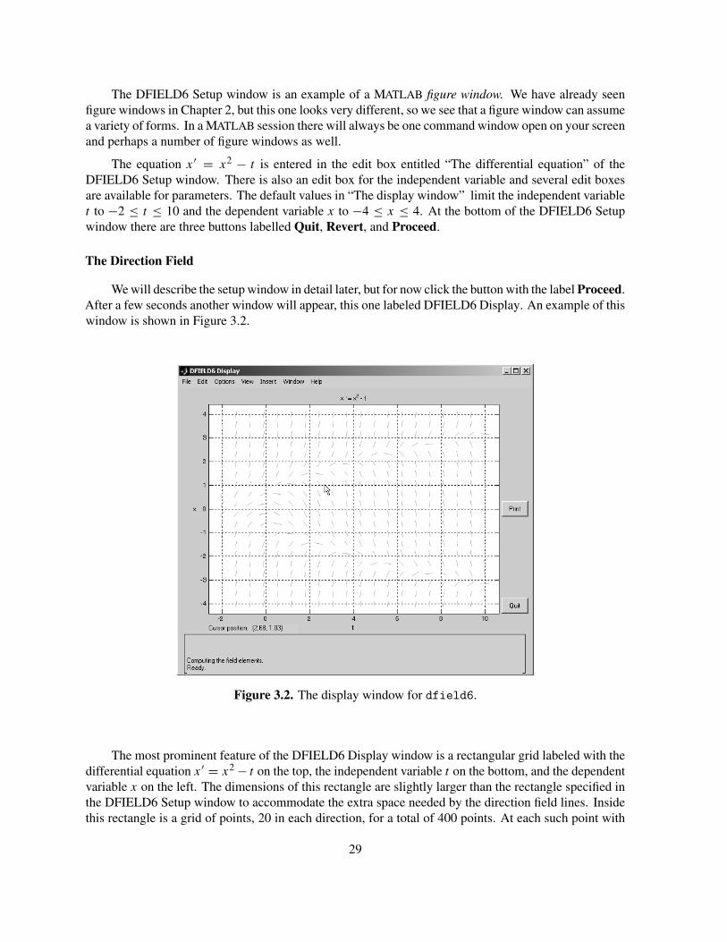
We will describe the setup window in detail later, but for now click the button with the label Proceed.After a few seconds another window will appear, this one labeled DFIELD6 Display. An example of thiswindow is shown in Figure 3.2.

Figure 3.2. The display window for dfield6.

The most prominent feature of the DFIELD6 Display window is a rectangular grid labeled with thedifferential equation x′ = x2 − t on the top, the independent variable t on the bottom, and the dependentvariable x on the left. The dimensions of this rectangle are slightly larger than the rectangle specified inthe DFIELD6 Setup window to accommodate the extra space needed by the direction field lines. Insidethis rectangle is a grid of points, 20 in each direction, for a total of 400 points. At each such point with

29

coordinates (t, x) there is shown a small line segment centered at (t, x) with slope equal to x2 − t . Thiscollection of lines is a subset of the direction field.

There is a pair of buttons on the DFIELD6 Display window: Quit and Print. There are severalmenus: File, Edit, Options, Insert, and Help. Below the direction field there is a small window givingthe coordinates of the cursor, and a larger message window through which dfield6 will communicatewith us. Note that the last line of this window contains the word “Ready,” indicating that dfield6 isready to follow orders.

Initial Value Problems

The differential equation x′ = x2 − t is in normal form, meaning that the derivative x′ is expressedas a function of the independent variable t and the dependent variable x. You will notice from Figure 3.1that dfield6 requires the differential equation to be in normal form. Most differential equations haveinfinitely many solutions. In order to get a particular solution it is necessary to specify an initial condition.The differential equation with initial condition,

x′ = f (t, x), x(t0) = x0, (3.1)

is called an initial value problem.

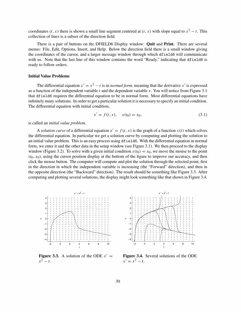
A solution curve of a differential equation x′ = f (t, x) is the graph of a function x(t) which solvesthe differential equation. In particular we get a solution curve by computing and plotting the solution toan initial value problem. This is an easy process using dfield6. With the differential equation in normalform, we enter it and the other data in the setup window (see Figure 3.1). We then proceed to the displaywindow (Figure 3.2). To solve with a given initial condition x(t0) = x0, we move the mouse to the point(t0, x0), using the cursor position display at the bottom of the figure to improve our accuracy, and thenclick the mouse button. The computer will compute and plot the solution through the selected point, firstin the direction in which the independent variable is increasing (the “Forward” direction), and then inthe opposite direction (the “Backward” direction). The result should be something like Figure 3.3. Aftercomputing and plotting several solutions, the display might look something like that shown in Figure 3.4.

−2 0 2 4 6 8 10

−4

−3

−2

−1

0

1

2

3

4

t

x

x ’ = x2 − t

−2 0 2 4 6 8 10

−4

−3

−2

−1

0

1

2

3

4

t

x

x ’ = x2 − t

Figure 3.3. A solution of the ODE x′ =x2 − t .

Figure 3.4. Several solutions of the ODEx′ = x2 − t .

30

Finer Control of Data. The next example illustrates several features of dfield6, including how to beaccurate with initial conditions.

Example 1. The voltage y on the capacitor in a certain RC circuit is modeled by the differential equationy′ +y = 3+ cos x, where we are using the variable x to represent time. Use dfield6 to plot the voltageover the interval 0 ≤ x ≤ 20, assuming that y(0) = 1.

You will notice that we are asked to solve the initial value problem

y′ + y = 3 + cos x, y(0) = 1. (3.2)

The dependent variable in this example is y and the independent variable is x. The differential equationy′ + y = 3 + cos x is not in normal form, so we put it in normal form by solving the equation for y′,getting y′ = −y + 3 + cos x.

Return to the DFIELD6 Setup window and select Edit→Clear all.2 Notice that there are optionson the Edit menu to clear particular regions of the DFIELD6 Setup window and each of these optionspossesses a keyboard accelerator. Enter the left and right sides of the differential equation y′ = −y +3+cos x, the independent variable (x in this case), and define the display window in the DFIELD6 Setupwindow as shown in Figure 3.5.3

Figure 3.5. The setup window for y′ = −y + 3 + cos x.

Should your data entry become hopelessly mangled, click the Revert button to restore the originalentries. The initial value problem in (3.2) contains no parameters, so leave the parameter fields in theDFIELD6 Setup window blank. Click the Proceed button to transfer the information in the DFIELD6Setup window to the DFIELD6 Display window and start the computation of the direction field.

Choosing the initial point for the solution curve with the mouse is convenient, but it is often difficultto be accurate, even with the help of the cursor position display. Instead, in the DFIELD6 Display window,select Options→Keyboard input. Enter the initial condition, y(0) = 1, as shown in Figure 3.6. Click theCompute button in the DFIELD6 Keyboard input window to compute the trajectory shown in Figure 3.7.

2 We continue to use the notation Edit→Clear all to signify that you should select “Clear all” fromthe Edit menu.

3 MATLAB is case-sensitive. Thus, the variable Y is completely different from the variable y.

31

Figure 3.6. The initial condition y(0) = 1 starts the solution trajectory at (0, 1).

Notice that it is not necessary to specify a computation interval. However, you can specify one ifyou wish by clicking the “Specify a computation interval” checkbox in the DFIELD6 Keyboard Inputwindow (See Figure 3.6), and then filling in the starting and ending times of the desired solution interval.For example, start a solution trajectory with initial condition y(0) = 0, but set the computation intervalso that −π ≤ x ≤ π . Try it!

0 2 4 6 8 10 12 14 16 18 20

0

0.5

1

1.5

2

2.5

3

3.5

4

x

y

y ’ = − y + 3 + cos(x)

17.2 17.4 17.6 17.8 18 18.2 18.4 18.6 18.8

2.7

2.75

2.8

2.85

2.9

2.95

3

3.05

3.1

3.15

3.2

x

yy ’ = − y + 3 + cos(x)

Figure 3.7. Solution of y′ +y = 3+cos x,y(0) = 1.

Figure 3.8. Zooming in to find y(18).

Example 2. For the voltage y(x) computed in Example 1 find y(18), accurate to 2 decimal places.

From the graph of the solution in Figure 3.7 we can see that the voltage y(18) is approximately 3.However, this is not accurate enough. To get more accuracy, we will increase the resolution using thezoom tools in dfield6. Select Edit→Zoom in in the DFIELD6 Display window, then single-click the(left) mouse button in the DFIELD6 Display window near the point (18, 3). Additional “zooms” requirethat you revisit Edit→Zoom in before clicking the mouse button to zoom. There is a faster way to zoomin that is platform dependent. If you have a mouse with more than one button, click the right mousebutton at the zoom point (or control-click the left mouse button at the zoom point). On a Macintosh,option-click the mouse button at the zoom point.4 After performing a couple of zooms (results may vary

4 Mouse actions are platform dependent in dfield6. See the front and back covers of this manualfor a summary of mouse actions on various platforms.

32

on your machine), greater resolution is obtained. When you reach a point similar to Figure 3.8, you canuse the cursor position display to see that y(18) ≈ 2.96.

Existence and Uniqueness

It would be comforting to know in advance that a solution of an initial value problem exists, especiallyif you are about to invest a lot of time and energy in an attempt to find a solution. A second (but noless important) question is uniqueness: is there only one solution? Or does the initial value problemhave more than one solution? Fortunately, existence and uniqueness of solutions have been thoroughlyexamined and there is a beautiful theorem that we can use to answer these questions.

Theorem 1. Suppose that the function f (t, x) is defined in the rectangle R defined by a ≤ t ≤ b andc ≤ x ≤ d. Suppose also that f and ∂f/∂x are both continuous in R. Then, given any point (t0, x0) ∈ R,there is one and only one function x(t) defined for t in an interval containing t0 such that x(t0) = x0 andx′ = f (t, x). Furthermore, the function x(t) is defined both for t > t0 and for t < t0, at least until thegraph of x leaves the rectangle R through one of its four edges.5

Example 3. Use dfield6 to sketch the solution of the initial value problem

x′ = x2, x(0) = 1.

Set the display window so that −2 ≤ t ≤ 3 and −4 ≤ x ≤ 4.

Enter the differential equation x′ = x2, the independent variable t , and the display window ranges−2 ≤ t ≤ 3 and −4 ≤ x ≤ 4 in the DFIELD6 Setup window. Click Proceed to compute the directionfield. Select Options→Keyboard input in the DFIELD6 Display window and enter the initial conditionx(0) = 1 in the DFIELD6 Keyboard input window. If all goes well, you should produce an image similarto that in Figure 3.9.

The differential equation x′ = x2 is in the form x′ = f (t, x), with f (t, x) = x2. In addition,f (t, x) = x2 and ∂f/∂x = 2x are continuous on the rectangle R defined by −2 ≤ t ≤ 3 and −4 ≤ x ≤ 4.Therefore, Theorem 1 states that the initial value problem has a solution as shown in Figure 3.9, and thatthis solution is unique. Use the mouse to experiment. You will see that any other solution is parallel tothe first one and does not pass through the point (0, 1).

Theorem 1 does not make a definitive statement about the domain of a solution. For example, doesthe solution in Figure 3.9 exist for all t or does it reach positive infinity in a finite amount of time? Thisquestion cannot be answered by dfield6 alone, although it can provide a hint. Go back to the Setupwindow and change the display window to 0 ≤ t ≤ 1.5 and 0 ≤ x ≤ 40 in order to focus on the solutionin Figure 3.9 near t = 1. When we proceed to the display window and recompute the solution, we getthe result shown in Figure 3.10. This seems to indicate that the solution becomes infinite near t = 1. Tocheck this out, we solve the differential equation. The general solution is x(t) = 1/(C − t), where C

is an arbitrary constant. Substituting the initial condition x(0) = 1 into the equation x(t) = 1/(C − t),

5 The notation ∂f/∂x represents the partial derivative of f with respect to x. Suppose, for example,that f (t, x) = x2 − t . To find ∂f/∂x, think of t as a constant and differentiate with respect to x to obtain∂f/∂x = 2x. Similarly, to find ∂f/∂t , think of x as a constant and differentiate with respect to t to obtain∂f/∂t = −1.

33

−2 −1.5 −1 −0.5 0 0.5 1 1.5 2 2.5 3

−4

−3

−2

−1

0

1

2

3

4

t

x

x ’ = x2

0 0.5 1 1.5

0

5

10

15

20

25

30

35

40

t

x

x ’ = x2

Figure 3.9. The solution of dx/dt = x2,x(0) = 1 is unique.

Figure 3.10. The solution “blows up” att = 1.

we find that 1 = 1/(C − 0), or C = 1, so the solution is x(t) = 1/(1 − t). From this equation, we seethat limt→1− x(t) = +∞. Mathematicians like to say that the solution “blows up” at t = 1.6 In thisparticular case, if the independent variable t represents time (in seconds), then the solution trajectoryreaches positive infinity when one second of time elapses.

Example 4. Consider the differential equation

dx

dt= x2 − t.

Sketch solutions with initial conditions x(2) = 0, x(3) = 0, and x(4) = 0. Determine whether or notthese solution curves intersect in the display window defined by −2 ≤ t ≤ 10 and −4 ≤ x ≤ 4.

Go to the setup window and select Gallery→default equation. The correct data will be entered.Click Proceed to transfer this information and begin computation of the direction field in the DFIELD6Display window. Select Options→Keyboard input in the DFIELD6 Display window and computesolutions for each of the initial conditions x(2) = 0, x(3) = 0, and x(4) = 0. If all goes well, you shouldproduce an image similar to that in Figure 3.11.

The ODE x′ = x2 − t is in normal form, x′ = f (t, x), with f (t, x) = x2 − t . Both f and∂f/∂x = 2x are continuous on the display window defined by −2 ≤ t ≤ 10 and −4 ≤ x ≤ 4. InFigure 3.11, it appears that the solution trajectories merge into one trajectory near the point (6, −2.4) (orperhaps even sooner). However, Theorem 1 guarantees that solutions cannot cross or meet in the displaywindow of Figure 3.11.

This situation can be analyzed by zooming in near the point (6, −2.4). After performing numerouszooms, some separation in the trajectories begins to occur, as shown in Figure 3.12. Without Theorem 1,we might have mistakenly assumed that the trajectories merged into one trajectory.

It is also possible to zoom in by dragging a “zoom box”. If you have a two button mouse, this canbe done by depressing the right mouse button, then dragging the mouse. Once the zoom box is drawn

6 The graph of the solution reaches infinity (or negative infinity) in a finite time period.

34

−2 0 2 4 6 8 10

−4

−3

−2

−1

0

1

2

3

4

t

x

x ’ = x2 − t

5.9996 6 6.0004

−2.406

−2.4055

−2.405

t

x

x ’ = x2 − t

Figure 3.11. Do the trajectories intersect? Figure 3.12. The trajectories don’t mergeor cross.

around the area of interest, release the mouse button and the contents of the zoom box will be magnifiedto the full size of the display window. The same effect can be achieved on a Macintosh with a one buttonmouse by depressing the option key while clicking and dragging.

Dfield6 allows you to “zoom back” to revisit any previously used window. Select Edit→Zoomback in the DFIELD6 Display window. This will open the DFIELD6 Zoom back dialog box pictured inFigure 3.13. Select the window you wish to revisit and click the Zoom button.

Figure 3.13. Select a zoom window and click the Zoom button.

Qualitative Analysis

Suppose that you model a population with a differential equation. If you want to use your model topredict the exact population in three years, then you will need to find an analytic or a numerical solution.However, if your only interest is what happens to the population after a long period of time, a qualitativeapproach might be easier and more appropriate.

Example 5. Let P(t) represent a population of bacteria at time t , measured in millions of bacteria.

35

Suppose that P is governed by the logistic model

dP

dt= rP

(

1 − P

K

)

. (3.3)

Assume that r = 0.75 and K = 10 and suppose that the initial population at time t = 0 is P(0) = 1.What will happen to this population over a long period of time?

Let’s first examine the model experimentally using dfield6. Instead of filling out the DFIELD6Setup window by hand, we can use the gallery by choosing Gallery→logistic equation. Notice that theparameters r and K have been given the correct values. To provide more room below P = 0, set theminimum value of P to be −4, as shown in Figure 3.14. Click the Proceed button to start the computationof the direction field.

Figure 3.14. Setup window for dP/dt = rP (1 − P/K).

Plot a few solutions by clicking the mouse at various points with P > 0. Notice that each of thesesolutions tends to 10 as t increases. Remember that K = 10. This is not a coincidence, and we willreturn to this point later. Some solution curves are shown in Figure 3.15.

0 2 4 6 8 10 12 14 16 18 20

−4

−2

0

2

4

6

8

10

12

14

16

t

P

P ’ = r P (1 − P/K) r = 0.75 K = 10

0 KP

rP(1 − P/K) ( = dP/dt )

dP/dt < 0

P decreases

dP/dt > 0

P increases

dP/dt < 0

P decreases

Figure 3.15. Solutions to P ′ = rP (1 −P/K).

Figure 3.16. The plot of rP (1 − P/K)

versus P .

36

This behavior can be predicted quite easily using qualitative analysis. If you plot the right hand sideof equation (3.3) versus P (i.e., plot rP (1 − P/K) versus P ), the result is the inverted parabola seen inFigure 3.16. Set rP (1 − P/K) equal to zero to find that the graph crosses the P -axis in Figure 3.16 atP = 0 and P = K . These are called equilibrium points. It is easily verified that P(t) = K is a solutionof dP/dt = rP (1 − P/K) by substituting P(t) = K into each side of the differential equation andsimplifying. Similarly, the solution P(t) = 0 is easily seen to satisfy the differential equation.

Although the solutions P(t) = 0 and P(t) = K might be considered “trivial” since they are constantfunctions, they are by no means trivial in their importance. The solutions P(t) = 0 and P(t) = K arecalled equilibrium solutions. For example, if P(t) = K , the growth rate dP/dt of the population is zeroand the population remains at P(t) = K forever. Similarly, if P(t) = 0, the growth rate dP/dt equalszero and the population remains at P(t) = 0 for all time.

When the graph of rP (1−P/K) (which is equal to dP/dt if P is a solution) falls below the P -axisin Figure 3.16, then dP/dt < 0 and the first derivative test implies that P(t) is a decreasing functionof t . On the other hand, when the graph of rP (1 − P/K) rises above the P -axis in Figure 3.16, thendP/dt > 0 and P(t) is an increasing function of t . These facts are summarized by the arrows on the P

axis in Figure 3.16. This is an example of a phase line. The information on the phase line indicates thata population beginning between 0 and K million bacteria has to increase to the equilibrium value of K

million bacteria. If the starting population is greater than K million then the population decreases to K

million. For this reason the parameter K is called the carrying capacity.

Now let’s go back to the DFIELD6 Display window. Select Options→Keyboard input and startsolution trajectories with initial conditions P(0) = 0 and P(0) = 10. For the second trajectory youcan enter P = K instead of P = 10, since the use of parameters is allowed in the keyboard inputwindow. In Figure 3.15, note that these equilibrium solutions are horizontal lines. Select Options→Solution direction→Forward and Options→Show the phase line in the DFIELD6 Display window.Dfield6 aligns the phase line from Figure 3.16 in a vertical direction at the left edge of the directionfield in the DFIELD6 Display window. To see the motion along the phase line it is a good idea to slowthe computations. Choose Options→Solver settings and move the slider to less than 10 solutions stepsper second.

Next begin the solution with initial condition P(0) = 1 and note the action of the animated point onthe phase line. As the solution trajectory in the direction field approaches the horizontal line P = 10 = K ,the point on the phase line approaches equilibrium point P = 10 on the phase line, as shown in Figure 3.15.It would appear that a population with initial conditions and parameters described in the original problemstatement will have to approach 10 million bacteria with the passage of time.

If you chose to slow the computation, perhaps you noticed something you had seen only fleetinglybefore. When a computation is started, a new button labelled Stop appears on the DFIELD6 Displaywindow. If you click this button, the solution of the trajectory in the current direction is halted.

Experiment with some other initial conditions. Note that solutions beginning a little above or alittle below the equilibrium solution P = 10 tend to move back toward this equilibrium solution withthe passage of time. This is why the solution P = 10 is called an assymptotically stable equilibriumsolution. However, solutions beginning a little above or a little below the equilibrium solution P = 0tend to move away from this equilibrium solution with the passage of time. The solution P = 0 is calledan unstable equilibrium solution. You can review the results of our experiments in Figure 3.15.

37

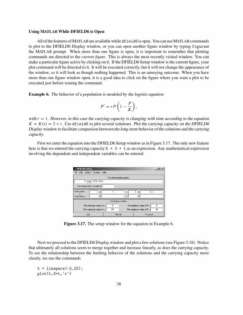
Using MATLAB While DFIELD6 is Open

All of the features of MATLAB are available whiledfield6 is open. You can use MATLAB commandsto plot to the DFIELD6 Display window, or you can open another figure window by typing figureatthe MATLAB prompt. When more than one figure is open, it is important to remember that plottingcommands are directed to the current figure. This is always the most recently visited window. You canmake a particular figure active by clicking on it. If the DFIELD6 Setup window is the current figure, yourplot command will be directed to it. It will be executed correctly, but it will not change the appearance ofthe window, so it will look as though nothing happened. This is an annoying outcome. When you havemore than one figure window open, it is a good idea to click on the figure where you want a plot to beexecuted just before issuing the command.

Example 6. The behavior of a population is modeled by the logistic equation

P ′ = rP

(

1 − P

K

)

,

with r = 1. However, in this case the carrying capacity is changing with time according to the equationK = K(t) = 3 + t. Use dfield6 to plot several solutions. Plot the carrying capacity on the DFIELD6Display window to facilitate comparison between the long-term behavior of the solutions and the carryingcapacity.

First we enter the equation into the DFIELD6 Setup window as in Figure 3.17. The only new featurehere is that we entered the carrying capacity K = 3 + t as an expression. Any mathematical expressioninvolving the dependent and independent variables can be entered.

Figure 3.17. The setup window for the equation in Example 6.

Next we proceed to the DFIELD6 Display window and plot a few solutions (see Figure 3.18). Noticethat ultimately all solutions seem to merge together and increase linearly, as does the carrying capacity.To see the relationship between the limiting behavior of the solutions and the carrying capacity moreclearly, we use the commands

t = linspace(-2,22);plot(t,3+t,'r')

38

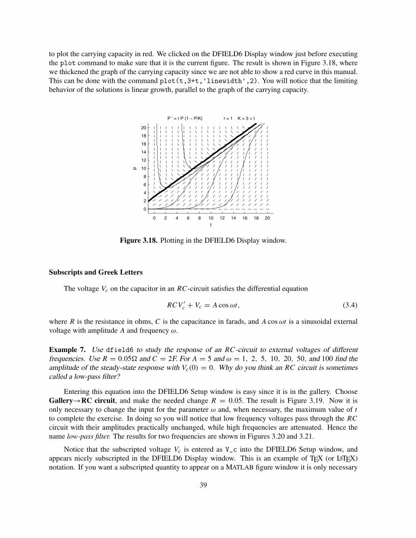
to plot the carrying capacity in red. We clicked on the DFIELD6 Display window just before executingthe plot command to make sure that it is the current figure. The result is shown in Figure 3.18, wherewe thickened the graph of the carrying capacity since we are not able to show a red curve in this manual.This can be done with the command plot(t,3+t,'linewidth',2). You will notice that the limitingbehavior of the solutions is linear growth, parallel to the graph of the carrying capacity.

0 2 4 6 8 10 12 14 16 18 20

0

2

4

6

8

10

12

14

16

18

20

t

P

P ’ = r P (1 − P/K) r = 1 K = 3 + t

Figure 3.18. Plotting in the DFIELD6 Display window.

Subscripts and Greek Letters

The voltage Vc on the capacitor in an RC-circuit satisfies the differential equation

RCV ′c + Vc = A cos ωt, (3.4)

where R is the resistance in ohms, C is the capacitance in farads, and A cos ωt is a sinusoidal externalvoltage with amplitude A and frequency ω.

Example 7. Use dfield6 to study the response of an RC-circuit to external voltages of differentfrequencies. Use R = 0.05� and C = 2F. For A = 5 and ω = 1, 2, 5, 10, 20, 50, and 100 find theamplitude of the steady-state response with Vc(0) = 0. Why do you think an RC circuit is sometimescalled a low-pass filter?

Entering this equation into the DFIELD6 Setup window is easy since it is in the gallery. ChooseGallery→RC circuit, and make the needed change R = 0.05. The result is Figure 3.19. Now it isonly necessary to change the input for the parameter ω and, when necessary, the maximum value of t

to complete the exercise. In doing so you will notice that low frequency voltages pass through the RC

circuit with their amplitudes practically unchanged, while high frequencies are attenuated. Hence thename low-pass filter. The results for two frequencies are shown in Figures 3.20 and 3.21.

Notice that the subscripted voltage Vc is entered as V_c into the DFIELD6 Setup window, andappears nicely subscripted in the DFIELD6 Display window. This is an example of TEX (or LATEX)notation. If you want a subscripted quantity to appear on a MATLAB figure window it is only necessary

39

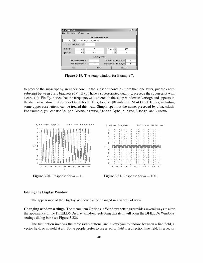
Figure 3.19. The setup window for Example 7.

to precede the subscript by an underscore. If the subscript contains more than one letter, put the entiresubscript between curly brackets ({}). If you have a superscripted quantity, precede the superscript witha caret (^). Finally, notice that the frequency ω is entered in the setup window as \omega and appears inthe display window in its proper Greek form. This, too, is TEX notation. Most Greek letters, includingsome upper case letters, can be treated this way. Simply spell out the name, preceded by a backslash.For example, you can use \alpha, \beta, \gamma, \theta, \phi, \Delta, \Omega, and \Theta.

0 10 20 30 40 50 60 70 80 90 100

−5

−4

−3

−2

−1

0

1

2

3

4

5

t

Vc

Vc ’ = (A cos(ω t) − V

c)/(R C) A = 5 ω = 1 R = 0.05 C = 2

0 0.5 1 1.5 2 2.5 3 3.5 4 4.5 5

−5

−4

−3

−2

−1

0

1

2

3

4

5

t

Vc

Vc ’ = (A cos(ω t) − V

c)/(R C) A = 5 ω = 100 R = 0.05 C = 2

Figure 3.20. Response for ω = 1. Figure 3.21. Response for ω = 100.

Editing the Display Window

The appearance of the Display Window can be changed in a variety of ways.

Changing window settings. The menu item Options→Windows settings provides several ways to alterthe appearance of the DFIELD6 Display window. Selecting this item will open the DFIELD6 Windowssettings dialog box (see Figure 3.22).

The first option involves the three radio buttons, and allows you to choose between a line field, avector field, or no field at all. Some people prefer to use a vector field to a direction line field. In a vector

40

Figure 3.22. DFIELD6 Window settings.

field, a vector is attached to each point instead of the line segment used in a direction field. The vectorhas its base at the point in question, its direction is the slope, and the length of the vector reflects themagnitude of the derivative. Click the Change settings button to make any change you select.

There is an edit box in the DFIELD6 Window settings dialog that allows the user to choose thenumber of field points displayed. The default is 20 points in each row and in each column. Change thisentry to 10, hit Enter, then click the Change settings button to note the affect on the direction field.

The design of dfield6 includes the definition of two windows: the DFIELD6 Display window andthe calculation window. When you start dfield6, the calculation window is 3.5 times as large as thedisplay window in each dimension. The computation of a solution will stop only when the solution curveleaves the calculation window. This allows some room for zooming to a larger display window withouthaving incomplete solution curves. It also allows for some reentrant solution curves — those which leavethe display window and later return to it. The third item in the DFIELD6 Window settings dialog boxcontrols the relative size of the calculation window. It can be given any value greater than or equal to1. The smaller this number the more likely that reentrant solutions will be lost. The default value of3.5 seems to meet most needs, but if you are losing too many reentrant solutions you can increase thisparameter.

Marking initial points. It is possible to mark the points at which the computation of solutions is started.To do this, select Options→Mark initial points. To stop doing so, select the same option to uncheck it.Initial points that are already plotted can be erased with the command Edit→Erase all marked initialpoints.

Level curves. Sometimes it is useful to plot level sets of functions in the DFIELD6 Display window.In Example 6, instead of plotting the curve P = K = 3 + t from the command line we could haveplotted the level curve P − K = 0. This can be done using the command Options→Plot level curves.Complete the window as shown in Figure 3.23 and click Proceed. If you want to remove the level sets,select Edit→Erase all level curves.

Erasing objects. Sometimes when you are preparing a display window for printing, you plot a solutioncurve you wish were not there. In the Edit menu there are several commands which allow you to eraseitems in the DFIELD6 Display window. In addition to those we have already explained, there are Edit→Erase all solutions and Edit→Erase all graphics objects, which are self explanatory. The last item,Edit→Delete a graphics object, is much more flexible. It will allow you to delete individual solutioncurves, as well as text items and graphs you have added to the window. Simply choose the option andselect the object you wish to delete with the mouse.

41

Figure 3.23. The DFIELD6 Level sets window.

Text objects in DFIELD6. The DFIELD6 Display window is a standard MATLAB figure window.Therefore all of the standard editing commands which we described in Chapter 2 are available. Inparticular the commands xlabel, ylabel, and title can be used to change these items. To add textat arbitrary points in the DFIELD6 Display window, select Edit→Enter text on the Display Window,enter the desired text in the Text entry dialog box, and then click the OK button. Use the mouse to clickat the lower left point of the position in the figure window where you want the text to appear. It can easilyhappen that your placement of the text does not please you. If so, remove the text using Edit→Delete agraphics object, then try again.

Using the Property Editors with DFIELD6. We described the use of the Property Editors in Chapter 2.While these methods are very powerful and not difficult to use, they do not mix flawlessly with theinteractive aspects of dfield6. You should be careful when you use them with the DFIELD6 Displaywindow. It is a good idea to complete all of your dfield6 work first, and only then begin to use theformatting commands. Do not mix them. It is not unusual that MATLAB freezes when the two are mixed.It is usually a good idea to select Options→Make the display window inactive before using the toolsin the toolbar.

Other Features of DFIELD6

Printing, Saving, and Using Clipboards. You can print or export the DFIELD6 Display window in anyof the ways described in Chapter 2. However, the easiest way to print the figure to the default printer isto click the Print button in the DFIELD6 Display window. The Print and Quit buttons and the messagewindow will not be printed.

Saving and Loading DFIELD6 Equation and Gallery Files. Suppose that after entering all of theinformation into the DFIELD6 Setup window for Example 7, as it appears in figure 3.19, you decided towork on something else and come back to this example later. There are two ways to avoid the necessity ofreentering the data. The first method is temporary. The menu option Gallery→Add current equationto the gallery will do just that, after prompting you for a name for the equation. When you are ready,you can choose this equation from the Gallery menu, and all of the data will be entered automatically.

However, if you have to quit dfield6, the new entry will no longer be there when you come back.For this situation you can use the command File→Save the current equation .... This option allowsyou to record the information on the DFIELD6 Setup window in a file. Executing this option will bringup a standard file save menu, where you are given the option of saving the file with a filename and in a

42

directory of your own choice. The file will be saved with the suffix .dfs. (It is not necessary to enter.dfs.) It can later be loaded back into dfield6 using the command File→Load an equation ....

It is also possible to save and load entire galleries using the appropriate commands on the File menu.Gallery files have the suffix .dfg. There is also a command that will delete the entire gallery, allowingyou to start to build a gallery entirely your own, and another command that will reload the default gallery,if that is what you want.

Quitting DFIELD6. Always wait until the word “Ready” appears in the dfield6 message windowbefore you try to do anything else with dfield6 or MATLAB. When you want to quit dfield6, the bestway is to use the Quit buttons found on the DFIELD6 Setup or on the DFIELD6 Display windows. Eitherof these will close all of the dfield6 windows in an orderly manner, and it will delete the temporaryfiles that dfield6 creates in order to do its business.

Plotting Several Solutions at Once. Dfield6 allows you to plot several solutions at once. SelectOptions→Plot several solutions and note that the mouse cursor changes to “cross-hairs” when positionedover the direction field. Select several initial conditions for your solutions by clicking the mouse buttonat several different locations in the direction field. When you are finished selecting initial conditions,position the mouse cross-hairs over the direction field and press the Enter or Return key on yourkeyboard. Solution trajectories will emanate from the initial conditions you selected with the mouse.

Exercises

For the differential equations in Exercises 1–4, perform each of the following tasks.

a) Print out the direction field for the differential equation with the display window defined by t ∈ [−5, 5]and y ∈ [−5, 5]. You might consider increasing the number of field points to 25 in the DFIELD6 Windowsettings dialog box. On this printout, sketch with a pencil as best you can the solution curves through theinitial points (t0, y0) = (0, 0), (−2, 0), (−3, 0), (0, 1), and (4, 0). Remember that the solution curvesmust be tangent to the direction lines at each point.

b) Use dfield6 to plot the same solution curves to check your accuracy. Turn in both versions.

1. y ′ = ty.

2. y ′ = y2 − t2.

3. y ′ = 2ty/(1 + y2).

4. y ′ = y(2 + y)(2 − y).

5. Use dfield6 to plot a few solution curves to the equation x ′ + x sin(t) = cos(t). Use the display windowdefined by x ∈ (−10, 10) and t ∈ (−10, 10).

6. Use dfield6 to plot the solution curves for the equation x ′ = 1 − t2 + sin(tx) with initial values x =−3, −2, −1, 0, 1, 2, 3 at t = 0. Find a display window which shows the most important features of thesolutions by experimentation.

For the differential equations in Exercises 7–10 perform the following tasks.

a) Use dfield6 to plot a few solutions with different initial points. Start with the display window boundedby 0 ≤ t ≤ 10 and −5 ≤ y ≤ 5, and modify it to suit the problem. Print out the display window and turnit in as part of this assignment.

b) Make a conjecture about the limiting behavior of the solutions of as t → ∞.

c) Find the general analytic solution to this equation.

d) Verify the conjecture you made in part b), or if you no longer believe it, make a new conjecture and verifythat.

43

7. y ′ + 4y = 8.

8. (1 + t2)y ′ + 4ty = t.

9. ty ′ + ty = 2 − y.

10. (1 + t)y ′ = y(4 − y2).

In Exercises 11–14 we will consider a certain lake which has a volume of V = 100 km3. It is fed by a river at a rate ofri km3/year, and there is another river which is fed by the lake at a rate which keeps the volume of the lake constant.In addition, there is a factory on the lake which introduces a pollutant into the lake at the rate of p km3/year. Thismeans that the rate of flow from the lake into the outlet river is (p + ri) km3/year. Let x(t) denote the volume of thepollutant in the lake at time t , and let c(t) = x(t)/V denote the concentration of the pollutant.

11. Show that, under the assumption of immediate and perfect mixing of the pollutant into the lake water, theconcentration satisfies the differential equation c′ + ((p + ri)/V )c = p/V .

12. Suppose that ri = 50, and p = 2.

a) Assume that the factory starts operating at time t = 0, so that the initial concentration is 0. Usedfield6 to plot the solution. Remember the definition of the concentration is x/V so you can be sureit is pretty small. Choose the dimensions of the display window carefully.

b) It has been determined that a concentration of over 2% is hazardous for the fish in the lake. Approxi-mately how long will it take until this concentration is reached? You can “zoom in” on the dfield6

plot to enable a more accurate estimate.

c) What is the limiting concentration? About how long does it take for the concentration to reach aconcentration of 3.5%?

13. Suppose the factory stops operating at time t = 0, and that the concentration was 3.5% at that time. Approx-imately how long will it take before the concentration falls below 2%, and the lake is no longer hazardous forfish? Notice that p = 0 for this exercise.

14. Rivers do not flow at the same rate the year around. They tend to be full in the Spring when the snow melts,and to flow more slowly in the Fall. To take this into account, suppose the flow of our river is

ri = 50 + 20 cos(2π(t − 1/3)).

Our river flows at its maximum rate one-third into the year, i.e., around the first of April, and at its minimumaround the first of October.

a) Setting p = 2, and using this flow rate, use dfield6 to plot the concentration for several choices ofinitial concentration between 0% and 4%. (If your solution seems erratic, reduce the relative errortolerance using Options→Solver settings.) How would you describe the behavior of the concentrationfor large values of time?

b) It might be expected that after settling into a steady state, the concentration would be greatest when theflow was smallest, around the first of October. At what time of the year does the highest concentrationactually occur? Reduce the error tolerance until you get a solution curve smooth enough to make anestimate.

15. Use dfield6 to plot several solutions to the equation z′ = (z − t)5/3. (Hint: Notice that when z < t ,z′ < 0, so the direction field should point down, and the solution curves should be decreasing. You mighthave difficulty getting the direction field and the solutions to look like that. If so read the section in Chapter1 on complex arithmetic, especially the last couple of paragraphs.)

A differential equation of the form dx/dt = f (x), whose right-hand side does not explicitly depend on the inde-pendent variable t , is called an autonomous differential equation. For example, the logistic model in Example 5 wasautonomous. For the autonomous differential equations in Exercises 16 – 19, perform each of the following tasks.Note that the first three tasks are to be performed without the aid of technology.

a) Set the right-hand side of the differential equation equal to zero and solve for the equilibrium points.

b) Plot the graph of the right-hand side of each autonomous differential equation versus x, as in Figure 3.16.Draw the phase line below the graph and indicate where x is increasing or decreasing, as was done inFigure 3.16.

44

c) Use the information in parts a) and b) to draw sample solutions in the xt plane. Be sure to include theequilibrium solutions.

d) Check your results with dfield6. Again, be sure to include the equilibrium solutions.

e) If x0 is an equilibrium point, i.e., if f (x0) = 0, then x(t) = x0 is an equilibrium solution. It can beshown that if f ′(x0) < 0, then every solution curve that has an initial value near x0 converges to x0 ast → ∞. In this case x0 is called a stable equilibrium point. If f ′(x0) > 0, then every solution curve thathas an initial value near x0 diverges away from x0 as t → ∞, and x0 is called an unstable equilibriumpoint. If f ′(x0) = 0, no conclusion can be drawn about the behavior of solution curves. In this case theequilibrium point may fail to be either stable or unstable. Apply this test to each of the equilibrium points.

16. x ′ = cos(πx), x ∈ [−3, 3].

17. x ′ = x(x − 2), −∞ < x < ∞.

18. x ′ = x(x − 2)2, −∞ < x < ∞.

19. x ′ = x(x − 2)3, −∞ < x < ∞.

In Exercises 20 – 22 you will not be able to solve explicitly for all of the equilibrium points. Instead, turn theproblem around. Use dfield6 to plot some solutions, and from that information calculate approximately where theequilibrium points are, and determine the type of each. In Exercise 20 you can check your estimate with the code:

f=inline('x*(1+exp(-x)-x^2)')z=fzero(f,1)

f(z)

Similar methods will help for Exercises 21 and 22.

20. x ′ = x(1 + e−x − x2), −1 ≤ x ≤ 2.

21. x ′ = x3 − 3x + 1.

22. x ′ = cos x − 2x.

The logistic equation P ′ = r P (1 − P/K) is discussed in Examples 5 and 6. Usually the parameter’s r and K areconstants and in Example 5 we found that for any solution P(t) which has a positive initial value we have P(t) → Kas t → ∞. For this reason K is called the carrying capacity of the system. However, in Example 6 we saw a casewhere the carrying capacity is not constant, yet we were able to show how the limiting behavior of the populationrelated to the carrying capacity. In Exercises 23–26 you are to examine the long term behavior of solutions, especiallyin comparison to the carrying capacity. In particular:

a) Use dfield6 to plot several solutions to the equation. (It is up to you to find a display window that isappropriate to the problem at hand.)

b) Based on the plot done in part a), describe the long term behavior of the solutions to the equation. Inparticular, compare this long term behavior to that of K . It might be helpful to plot K on the displaywindow as we did in Example 6. In the first case the solutions will all be asymptotic to a constant. In theother two the solutions will all have the same long term behavior. Describe that behavior in comparisonto the graph of K . The results of Examples 5 and 6 should be helpful.

23. K(t) = 1 − 12 e−t , r = 1. In this case K(t) is monotone increasing, and K(t) is asymptotic to 1. This

might model a situation of a human population where, due to technological improvement, the availability ofresources is increasing with time, although ultimately limited.

24. K(t) = √1 + t , r = 1. Again K(t) is monotone increasing, but this time it is unbounded. This might model

a situation of a human population where, due to technological improvement, the availability of resources issteadily increasing with time, and therefore the effects of competition are becoming less severe.

25. K(t) = 1 − 12 cos(2πt), r = 1. This is perhaps the most interesting case. Here the carrying capacity is

periodic in time with period 1, which should be considered to be one year. This models a population of insectsor small animals that are affected by the seasons. You will notice that the long term behavior as t → ∞reflects the behavior of K . The solution does not tend to a constant, but nevertheless all solutions have thesame long term behavior for large values of t . In particular, you should take notice of the location of the

45

maxima and minima of K and of P and how they are related. You can use the “zoom in” option to get a betterpicture of this.

26. K(t) = √1 + t − 1

2 cos(2πt), r = 1.

27. Despite the seeming generality of the uniqueness theorem, there are initial value problems which have morethan one solution. Consider the differential equation y ′ = √|y|. Notice that y(t) ≡ 0 is a solution with theinitial condition y(0) = 0. (Of course by

√|y| we mean the nonnegative square root.)

a) This equation is separable. Use this to find a solution to the equation with the initial value y(t0) = 0assuming that y ≥ 0. You should get the answer y(t) = (t − t0)

2/4. Notice, however, that this is asolution only for t ≥ t0. Why?

b) Show that the function

y(t) ={

0, if t < t0;(t − t0)

2/4, if t ≥ t0;is continuous, has a continuous first derivative, and satisfies the differential equation y ′ = √|y|.

c) For any t0 ≥ 0 the function defined in part b) satisfies the initial condition y(0) = 0. Why doesn’t thisviolate the uniqueness part of the theorem?

d) Find another solution to the initial value problem in a) by assuming that y ≤ 0.

e) You might be curious (as were the authors) about what dfield6 will do with this equation. Find out.Use the rectangle defined by −1 ≤ t ≤ 1 and −1 ≤ y ≤ 1 and plot the solution of y ′ = √|y| withinitial value y(0) = 0. Also, plot the solution for y(0) = 10−50 (the MATLAB notation for 10−50 is1e-50). Plot a few other solutions as well. Do you see evidence of the non-uniqueness observed inpart c)?

An important aspect of differential equations is the dependence of solutions on initial conditions. There are twopoints to be made. First, we have a theorem which says that the solutions are continuous with respect to the initialconditions. More precisely,

Theorem. Suppose that the function f (t, x) is defined in the rectangle R defined by a ≤ t ≤ b and c ≤ x ≤ d.Suppose also that f and ∂f /∂x are both continuous in R, and that

∣

∣

∣

∣

∂f

∂x

∣

∣

∣

∣

≤ L for all (t, x) ∈ R.

If (t0, x0) and (t0, y0) are both in R, and if

x ′ =f (t, x)

x(t0) =x0

andy ′ =f (t, y)

y(t0) =y0

then for t > t0

|x(t) − y(t)| ≤ eL(t−t0)|x0 − y0|as long as both solution curves remain in R.

Roughly, the theorem says that if we have initial values that are sufficiently close to each other, the solutions willremain close, at least if we restrict our view to the rectangle R. Since it is easy to make measurement mistakes, andthereby get initial values off by a little, this is reassuring.

For the second point, we notice that although the dependence on the initial condition is continuous, the term eL(t−t0)

allows the solutions to get exponentially far apart as the interval between t and t0 increases. That is, the solutionscan still be extremely sensitive to the initial conditions, especially over long t intervals.

28. Consider the differential equation x ′ = x(1 − x2).

a) Verify that x(t) ≡ 0 is the solution with initial value x(0) = 0.

46

b) Use dfield6 to find approximately how close the initial value y0 must be to 0 so that the solution y(t)of our equation with that initial value satisfies y(t) ≤ 0.1 for 0 ≤ t ≤ tf , with tf = 2. You can usethe display window 0 ≤ t ≤ 2, and 0 ≤ x ≤ 0.1, and experiment with initial values in the Options→Keyboard input window, until you get close enough. Do not try to be too precise. Two significantfigures is sufficient.

c) As the length of the t interval is increased, how close must y0 be to 0 in order to insure the sameaccuracy? To find out, repeat part b) with tf = 4, 6, 8, and 10.

The results of the last problem show that the solutions can be extremely sensitive to changes in the initial conditions.This sensitivity allows chaos to occur in deterministic systems, which is the subject of much current research.

One way to experience first hand the sensitivity to changes in the initial conditions is to try a little “target practice.”For the ODEs in Exercises 29–33, use dfield6 to find approximately the value of x0 such that the solution x(t)to the initial value problem with initial condition x(0) = x0 satisfies x(t1) = x1. You should use the Keyboardinput window to initiate the solution. Widen the window to allow a large number of digits in the edit window byclicking and dragging on the right edge. After an unsuccessful attempt try again with another initial condition. TheUniqueness Theorem should help you limit your choices. If you make sure that the Display Window is the currentfigure (by clicking on it), and execute plot(t1,x1,'or') at the command line, you will have a nice target to shootat.

You will find that hitting the target gets more difficult in each of these problems. We allow you to “cheat” by startinga solution in the target, and finding the value at t = 0. However, be sure to try to hit the target with that initial value.You may be surprised at the outcome.

29. x ′ = x − sin(x), t1 = 5, x1 = 2.

30. x ′ = x2 − t , t1 = 4, x1 = 0.

31. x ′ = x(1 − x2), t1 = 5, x1 = 0.5.

32. x ′ = x sin(x) + t , t1 = 5, x1 = 0.

33. x ′ = x sin(x2) + t , t1 = 5, x1 = 1. In this case the authors were not able to hit the target. However, theexercise of trying is still worthwhile. We leave it to you to ponder why it is not possible.

Appendix: Downloading and Installing the Software Used in This Manual

The MATLAB programs dfield, pplane, and odesolve, and the solvers eul, rk2, and rk4described in this manual are not distributed with MATLAB. They are MATLAB function M-files and areavailable for download over the internet. There are versions of dfield and pplane written for use withall recent versions of MATLAB. However, odesolve is new, and only works with MATLAB ver 6.0 andlater. The solvers are the same for all versions of MATLAB.

The following three step procedure will insure a correct installation, but the only important point isthat the files must be saved as MATLAB M-files in a directory on the MATLAB path.

• Create a new directory with the name odetools (or choose a name of your own). It can be locatedanywhere on your directory tree, but put it somewhere where you can find it later.

• In your browser, go to http://math.rice.edu/~dfield/. For each file you wish to download,click on the link. In Internet Explorer, you are given the option to save the file. In Netscape, the filefor the software will open in your browser, and you can save the file using the File menu. In eithercase, save the file with the subscript .m in the directory odetools.

• Open the path tool by executing the command pathtool in the MATLAB command window, or byselecting File→Set Path .... Follow the instructions for adding the directory odetools to the path.If you are asked if you want the change to be permanent, say yes.

From this point on, the programs will be available in MATLAB.

47

4. The Use of Function M-Files

In Chapter 2 we discussed script M-files, and how they can be used to facilitate the preparation ofcomplicated graphics. Here we will introduce function M-files, which are very like script M-files, butcan pass parameters and isolate variables. These two capabilities can be exploited to add new functionsto MATLAB’s already extensive list, and to extend our ability to perform computational experiments andprepare graphics.

In this chapter we will emphasize the use of MATLAB’s built-in editor. If you use a different editor,and one of the authors does, then ignore these parts. However, the MATLAB editor has several connectionswith MATLAB iself that make it a good choice.

New Functions in MATLAB

It is very easy to add your own functions to the long list provided by MATLAB. Let’s start with avery easy example.

Example 1. Create a function M-file for the function f (x) = x2 − 1.

Execute edit at the command line to open the MATLAB editor1 and enter the following three lines(one of them is blank, and is provided for readability):

function y = f(x)

y = x^2-1;

The first line of a function M-file must conform to the indicated format. It is this first line that distinguishesbetween a function M-file and a script M-file. The very first word must be the word function. The restof the first line has the form

dependent_variables = function_name(independent_variables)

In the function f, y = f(x) indicates that x is the independent variable and y is the dependent variable.

The rest of the function M-file defines the function using the same syntax we have been using atthe MATLAB prompt. Remember to put a semicolon at the end of lines in which computations are done.Otherwise the results will be printed in the Command Window.

When you save the file, you will be prompted to use the file name f.m. The file name should alwaysbe the same as the function name, followed by the suffix .m, so accept the suggestion. That’s all there isto it. Now if you want to compute f (3) = (3)2 − 1 = 8, simply enter f(3) at the MATLAB prompt.

>> f(3)ans =

8

1 There are several ways to open the editor. Explore the Toolbar and the Edit menu.

48

Making Functions Array Smart. There is one important enhancement you will want to make to theM-file f.m. If you try to compute f on a matrix or a vector, you will find that it is not array smart.

>> x = 1:5x =

1 2 3 4 5>> f(x)??? Error using ==> ^Matrix must be square.

This error message refers to the fact that we tried to compute x^2 for a vector x. We forgot to use arrayexponentiation instead of ordinary exponentiation. To edit the function to make it array smart we simplyadd one period:

function y = f(x)

y = x.^2-1;

Now the function can handle matrices. With the same vector x, we get

>> f(x)ans =

0 3 8 15 24

Notice that if x is a matrix, then so is x.^2. On the other hand, 1 is a number, so the difference x.^2-1is not defined in ordinary matrix arithmetic. However, MATLAB allows it, and in cases like this willsubtract 1 from every element of the matrix. This is a very useful feature in MATLAB.

Example 2. An object thrown in the air obeys the initial value problem

d2y

dt2= −9.8 − dy

dt, with y(0) = 0 and y′(0) = 120.

When we solve this linear equation, we find that

y = −49

5t + 649

5

(

1 − e−t)

,

where y is the height in meters of the object above ground level after t seconds. Estimate the height ofthe ball after 5 seconds.

This is a perfect situation for a function M-file, particularly if you are interested in predicting theheight of the ball at a number of additional times other than t = 5 seconds. Open a new M-file in theeditor, enter

function y = height(t)y = -(49/5)*t + (649/5)*(1 - exp(-t));

49

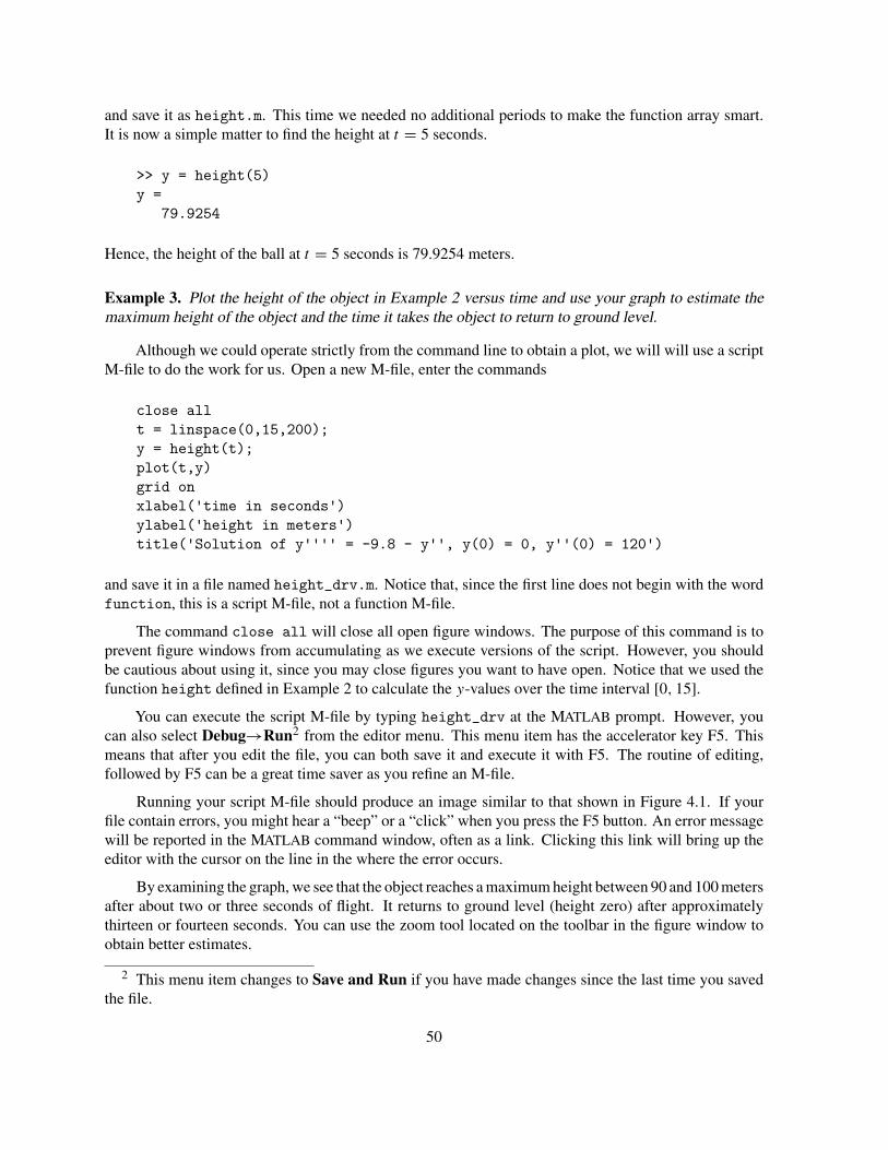
and save it as height.m. This time we needed no additional periods to make the function array smart.It is now a simple matter to find the height at t = 5 seconds.

>> y = height(5)y =

79.9254

Hence, the height of the ball at t = 5 seconds is 79.9254 meters.

Example 3. Plot the height of the object in Example 2 versus time and use your graph to estimate themaximum height of the object and the time it takes the object to return to ground level.

Although we could operate strictly from the command line to obtain a plot, we will will use a scriptM-file to do the work for us. Open a new M-file, enter the commands

close allt = linspace(0,15,200);y = height(t);plot(t,y)grid onxlabel('time in seconds')ylabel('height in meters')title('Solution of y'''' = -9.8 - y'', y(0) = 0, y''(0) = 120')

and save it in a file named height_drv.m. Notice that, since the first line does not begin with the wordfunction, this is a script M-file, not a function M-file.

The command close all will close all open figure windows. The purpose of this command is toprevent figure windows from accumulating as we execute versions of the script. However, you shouldbe cautious about using it, since you may close figures you want to have open. Notice that we used thefunction height defined in Example 2 to calculate the y-values over the time interval [0, 15].

You can execute the script M-file by typing height_drv at the MATLAB prompt. However, youcan also select Debug→Run2 from the editor menu. This menu item has the accelerator key F5. Thismeans that after you edit the file, you can both save it and execute it with F5. The routine of editing,followed by F5 can be a great time saver as you refine an M-file.

Running your script M-file should produce an image similar to that shown in Figure 4.1. If yourfile contain errors, you might hear a “beep” or a “click” when you press the F5 button. An error messagewill be reported in the MATLAB command window, often as a link. Clicking this link will bring up theeditor with the cursor on the line in the where the error occurs.

By examining the graph, we see that the object reaches a maximum height between 90 and 100 metersafter about two or three seconds of flight. It returns to ground level (height zero) after approximatelythirteen or fourteen seconds. You can use the zoom tool located on the toolbar in the figure window toobtain better estimates.

2 This menu item changes to Save and Run if you have made changes since the last time you savedthe file.

50

0 5 10 15−20

0

20

40

60

80

100

time in seconds

heig

ht in

met

ers

Solution of y’’ = −9.8 − y’, y(0) = 0, y’(0) = 120

Figure 4.1. Plotting the solution of y′′ = −9.8 − y′, y(0) = 0, y′(0) = 120.

Function M-files, Computational Exercises and Graphics

Some of you might wonder why we had to use both the function M-file height.m and the script M-file height_drv.m to produce Figure 4.1 in Example 2. It takes time to write files, and the accumulationof files clutters up the directory in which they are saved. Starting with version 6 of MATLAB there is away around this problem.

Subfunctions in MATLAB 6. The answer is to define the function height as a subfunction with the fileheight_drv.m. However, subfunctions are not allowed in script M-files.

Open MATLAB’s built-in editor, enter

function ch4examp3close allt = linspace(0,15,200);y = height(t);plot(t,y)grid onxlabel('time in seconds')ylabel('height in meters')title('Solution of y'''' = -9.8 - y'', y(0) = 0, y''(0) = 120')

function y = height(t)y = -(49/5)*t + (649/5)*(1 - exp(-t));

and save it as ch4examp3.m. Use the F5 key to execute the file. This should produce a plot similar tothat in Figure 4.1.

Notice that the code in ch4examp3 is precisely the same as the code in the two files height.m andheight_drv.m created in Examples 2 and 3. However, this is a single function M-file with heightincluded as a subfunction.

51

Functions of functions — MATLAB’s funfun directory. MATLAB has a large number of functionsthat act on functions. If you type

>> help funfun

at MATLAB’s prompt, you will see a list of MATLAB routines for finding zeros and extrema of functions,tools for numerical integration, and many others. There is a suite of routines for solving differentialequations, which we will look at in Chapter 8. For help on any of these functions, say fzero, executehelp fzero and learn how to find the zeros of a function.

Example 4. Use fzero to find the time it takes the object in Example 2 to return to ground level.

The help command indicates that “X = FZERO(FUN,X0) tries to find a zero of the function FUNnear X0.” Thus, fzero needs two inputs, the name of a function, and an approximate value of the zero.We will use the function height from Example 2, and from Figure 4.1 we estimate that height has azero near t = 13. In all versions of MATLAB you can invoke fzero with the command

>> t = fzero('height',13)t =

13.2449

Notice that the function name must be entered between single quotes. Starting with version 6 of MATLAB,the use of

>> t = fzero(@height,13)t =

13.2449

is encouraged. The expression @height is a function handle for the function height. In either case, wefind that the object returns to ground level after about 13.2 seconds. This certainly agrees with that wesee in Figure 4.1.

Example 5. Find the maximum height reached by the object in Example 2.

In the list provided by help funfunwe find that MATLAB doesn’t provide a function for finding themaximum of a function. However, the routine fminbnd will find a local minimum, and a local maximumof a function can be determined by finding a local minimum of the negative of the function.

Using help fminbnd, we learn that finding the minimum of a function on a given interval requiresthe input of a function and the beginning and endpoints of the interval in which to find the minimum.Consequently, we will apply fminbnd to the negative of height on the interval [0, 5]. One approachwould be to write a new function M-file encoding the negative of −(49/5)t +(649/5)(1−e−t ). However,let’s pursue an alternative.

MATLAB provides a perfect solution for the situation when you need a function, but do not wantto go to the trouble of writing a function M-file, called an inline function.3 We could create our inline

3 Type help inline to get a thorough explanation of the use of inline functions.

52

function for the negative of height as

>> f = inline('(49/5)*t - (649/5)*(1 - exp(-t))','t')f =

Inline function:f(t) = (49/5)*t - (649/5)*(1 - exp(-t))

However, since we have already created height, it is easier to use the inline function

>> f = inline('-height(t)','t')f =

Inline function:f(t) = -height(t)

From Figure 4.1 we estimate that the maximum occurs between t = 0 and t = 5, so the command

>> t = fminbnd(f,0,5)t =

2.5836

finds the time at which the maximum occurs. Notice that there are no single quotes around f infminbnd(f,1,5), so inline functions are treated differently from function M-files as inputs. Alterna-tively, the syntax t = fminbnd(inline('-height(t)'),1,5) will do the job in a single command.

The maximum height is now easily calculated by

>> h = -f(t)h =

94.6806

or by h = height(t). Compare these results with Figure 4.1.

Using function M-files to pass parameters. The ability of function M-files to have input variables canbe used to advantage when producing graphics. We will present a simple example.

Example 6. Write a function M-file that will plot the solution to the initial value problem

y′ + y = 2t cos t with y(0) = y0

over the interval [0, 4π ]. Write the file with y0 as an input variable.

The equation is linear, and we find that the general solution is y(t) = t (cos t + sin t)− sin t +Ce−t .

At t = 0, we find that y0 = y(0) = C. Thus the function M-file

function ch4examp6(y0)t = linspace(0,4*pi);y = t.*(cos(t) + sin(t)) - sin(t) + y0*exp(-t);plot(t,y), shg

53

will produce the required graph when ch4examp6(y0) is executed at the command line. Of course, youwill want to add formatting commands to your function M-file. The result is shown in Figure 4.2. Theone tricky formatting command is the one that produces the title. The command

title(['y'' + y = 2tcos(t) with y(0) = ', num2str(y0), '.'])

requires the concatenation of text strings, as explained in the section "Text Strings in MATLAB" inChapter 2.

0 2 4 6 8 10 12 14−15

−10

−5

0

5

10

15

t

y(t)

y’ + y = 2tcos(t) with y(0) = 11.

Figure 4.2. The output of ch4examp6(11).

Functions of Several Variables

MATLAB allows multiple input and output variables in function M-files.

Example 7. Write a function M-file for the function defined by f (t, x) = x2 − t .

We need to choose a name for this function, so let’s use the mnemonic xsqmt (“x squared minust”). Then the following M-file describes this function:

function y = xsqmt(t,x)% This is Example 7 of Chapter 4.y=x.^2-t;

The first line of the file starts with the word function. After that comes y=xsqmt(t,x), meaning thaty is the dependent variable, and both t and x are independent variables.

Everything on a line in an M-file after a percentage sign (%) is ignored by MATLAB. This can beutilized to put comments in a file, as we have done in the function xsqmt. Comment lines are usefulways to document your M-files. It is amazing how quickly we forget why we did things the way we did.Comment lines immediately after the function statement can be read using the MATLAB help command.

54

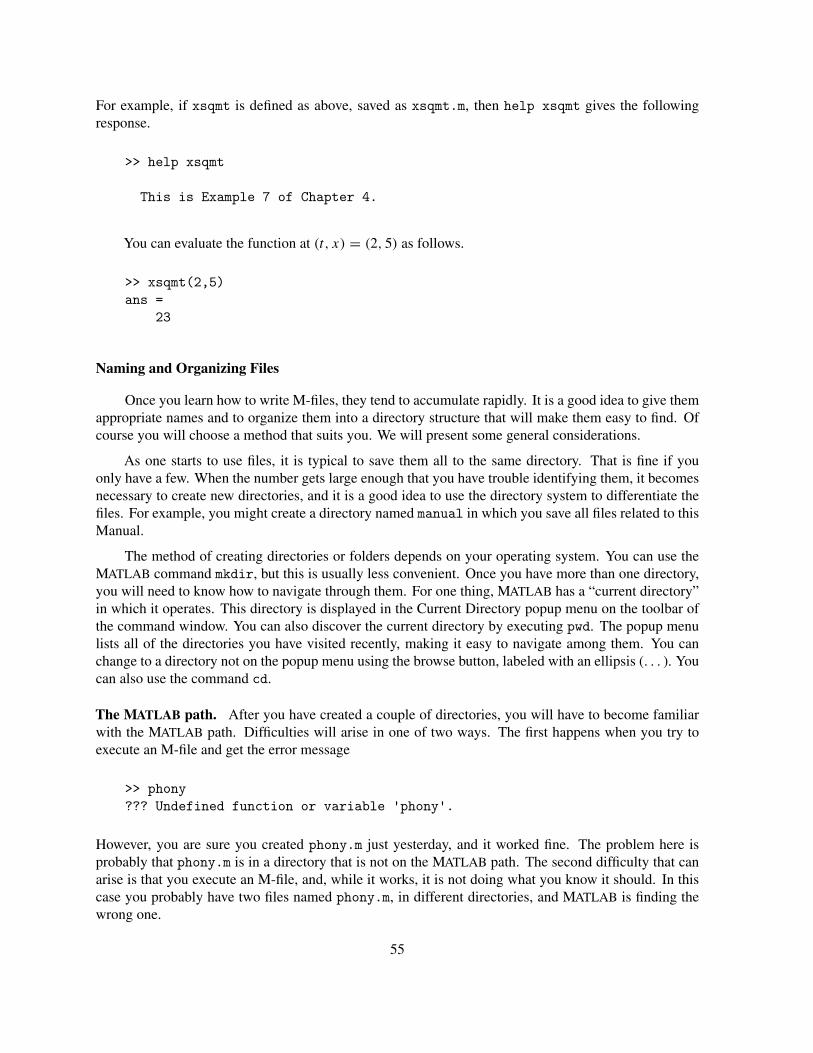
For example, if xsqmt is defined as above, saved as xsqmt.m, then help xsqmt gives the followingresponse.

>> help xsqmt

This is Example 7 of Chapter 4.

You can evaluate the function at (t, x) = (2, 5) as follows.

>> xsqmt(2,5)ans =

23

Naming and Organizing Files

Once you learn how to write M-files, they tend to accumulate rapidly. It is a good idea to give themappropriate names and to organize them into a directory structure that will make them easy to find. Ofcourse you will choose a method that suits you. We will present some general considerations.

As one starts to use files, it is typical to save them all to the same directory. That is fine if youonly have a few. When the number gets large enough that you have trouble identifying them, it becomesnecessary to create new directories, and it is a good idea to use the directory system to differentiate thefiles. For example, you might create a directory named manual in which you save all files related to thisManual.

The method of creating directories or folders depends on your operating system. You can use theMATLAB command mkdir, but this is usually less convenient. Once you have more than one directory,you will need to know how to navigate through them. For one thing, MATLAB has a “current directory”in which it operates. This directory is displayed in the Current Directory popup menu on the toolbar ofthe command window. You can also discover the current directory by executing pwd. The popup menulists all of the directories you have visited recently, making it easy to navigate among them. You canchange to a directory not on the popup menu using the browse button, labeled with an ellipsis (. . . ). Youcan also use the command cd.

The MATLAB path. After you have created a couple of directories, you will have to become familiarwith the MATLAB path. Difficulties will arise in one of two ways. The first happens when you try toexecute an M-file and get the error message

>> phony??? Undefined function or variable 'phony'.

However, you are sure you created phony.m just yesterday, and it worked fine. The problem here isprobably that phony.m is in a directory that is not on the MATLAB path. The second difficulty that canarise is that you execute an M-file, and, while it works, it is not doing what you know it should. In thiscase you probably have two files named phony.m, in different directories, and MATLAB is finding thewrong one.

55

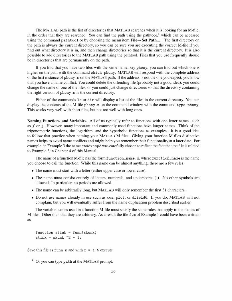
The MATLAB path is the list of directories that MATLAB searches when it is looking for an M-file,in the order that they are searched. You can find the path using the pathtool,4 which can be accessedusing the command pathtool or by choosing the menu item File→Set Path... . The first directory onthe path is always the current directory, so you can be sure you are executing the correct M-file if youfind out what directory it is in, and then change directories so that it is the current directory. It is alsopossible to add directories to the MATLAB path using the pathtool. Files that you use frequently shouldbe in directories that are permanently on the path.

If you find that you have two files with the same name, say phony, you can find out which one ishigher on the path with the command which phony. MATLAB will respond with the complete addressof the first instance of phony.m on the MATLAB path. If the address is not the one you expect, you knowthat you have a name conflict. You could delete the offending file (probably not a good idea), you couldchange the name of one of the files, or you could just change directories so that the directory containingthe right version of phony.m is the current directory.

Either of the commands ls or dir will display a list of the files in the current directory. You candisplay the contents of the M-file phony.m on the command window with the command type phony.This works very well with short files, but not too well with long ones.

Naming Functions and Variables. All of us typically refer to functions with one letter names, suchas f or g. However, many important and commonly used functions have longer names. Think of thetrigonometric functions, the logarithm, and the hyperbolic functions as examples. It is a good ideato follow that practice when naming your MATLAB M-files. Giving your function M-files distinctivenames helps to avoid name conflicts and might help you remember their functionality at a later date. Forexample, in Example 3 the name ch4examp3 was carefully chosen to reflect the fact that the file is relatedto Example 3 in Chapter 4 of this Manual.

The name of a function M-file has the form function_name.m, where function_name is the nameyou choose to call the function. While this name can be almost anything, there are a few rules.

• The name must start with a letter (either upper case or lower case).

• The name must consist entirely of letters, numerals, and underscores ( ). No other symbols areallowed. In particular, no periods are allowed.

• The name can be arbitrarily long, but MATLAB will only remember the first 31 characters.

• Do not use names already in use such as cos, plot, or dfield6. If you do, MATLAB will notcomplain, but you will eventually suffer from the name duplication problem described earlier.

The variable names used in a function M-file must satisfy the same rules that apply to the names ofM-files. Other than that they are arbitrary. As a result the file f.m of Example 1 could have been writtenas

function stink = funn(skunk)stink = skunk.^2 - 1;

Save this file as funn.m and with x = 1:5 execute

4 Or you can type path at the MATLAB prompt.

56

>> funn(x)ans =

0 3 8 15 24

Compare this to the output produced earlier with f(x) and note that there is no difference. It is importantto realize that the variable names used in function M-files are local to these files; i.e., they are notrecognized outside of the M-files themselves. See Exercises 12 and 13. In addition variables that havebeen defined at the command line are not available within function M-files. Script M-files, on the otherhand, do not isolate variables.

Exercises

Find the solution of each of the initial value problems in Exercises 1–4, then craft an inline function for the solution.After insuring that your inline function is “array smart,” use the inline function to (i) plot the solution of the initialvalue problem on the given interval, and (ii) evaluate the solution at the right endpoint of the given interval.

1. y ′ = −t/y, with y(0) = 4, on [0, 4].

2. y ′ = −2ty2, with y(0) = 1, on [0, 5].

3. y ′ + y = cos t , with y(0) = 1, on [0, 5π ].

4. y ′ + 2y = sin(2t), with y(0) = 1, on [0, 4π ].

Find the solution of each of the initial value problems in Exercises 5–8, then craft a function M-file for the solution.After insuring that your function M-file is “array smart,” use the function to (i) plot the solution of the initial valueproblem on the given interval, and (ii) evaluate the solution at the right endpoint of the given interval.

5. y ′ = (1 − t)y, with y(0) = 1, on [0, 4].

6. y ′ = y sin(2t), with y(0) = 1, on [0, 2π ].

7. y ′ = y/t + t , y(1) = −1, on [0, 3].

8. y ′ + t2y = 3, with y(0) = −2, on [0, 5].

Find the solution of the given initial value problem in Exercises 9–12, then craft a function M-file for the solution.After insuring that your function M-file is “array smart,” plot the solution on the given interval. Use MATLAB’sfminbnd function to find the minimum value of the solution on the given interval and the time at which it occurs.Use the figure window’s “Insert Text” and “Insert Arrow” tools to annotate your plot with these findings.5

9. y ′ + 2ty = −e−t2, with y(0) = 0, on [0, 2].

10. y ′ − y/t = −t sin t , with y(π) = −π , on [0, 2π ].

11. y ′ = 1 + 2y/t , with y(1) = −3/4, on [1, 4].

12. y ′ + y = t2, with y(0) = 1, on [0, 2].

Find the solution of the given initial value problem in Exercises 13–16, then craft a function M-file for the solution.After insuring that your function M-file is “array smart,” plot the solution on the given interval. Use MATLAB’sfminbnd function and the technique of Example 5 to find the maximum value of the solution on the given intervaland the time at which it occurs. Use the figure window’s “Insert Text” and “Insert Arrow” tools to annotate your plotwith these findings.

13. ty ′ − y = t2 cos(t), with y(π) = 0, on [0, 2π ].

14. y ′ = y cos(t), with y(0) = 1, on [0, 2π ].

15. y ′ = (1 + y) sin(t), with y(π) = 0, on [0, 2π ].

5 If the figure toolbar is not visible, select View→ Figure Toolbar from the figure menu.

57

16. y ′ + t2y = 3, with y(0) = 1, on [0, 3].

17. The differential equation y ′+y = cos(4t) has the general solution y = (1/17) cos(4t)+(4/17) sin(4t)+Ce−t .Craft a function M-file for this solution as follows.

function y = f(t,C)

y = 1/17*cos(4*t) + 4/17*sin(4*t) + C*exp(-t);

Plot a family of solutions for the differential equation with the following script.

t = linspace(0,2*pi,500);

y = [];

for C = -20:5:20

y = [y;f(t,C)];

end

plot(t,y)

Follow the lead of Exercise 17 to plot the given families of solutions in Exercises 18–23. Use the indicated constantsand extend your plot over the given time interval.

18. y = 2/(t2 + C), C = 1, 2, 3, 4, 5, on [−2, 2].

19. y = (1/4)t2 − (1/8)t + 1/32 + Ce−4t , C = 1, 2, 3, 4, 5, on [0, 2].

20. y = Cte−t2, C = −3, −2, −1, 0, 1, 2, 3, on [−2, 2].

21. y = (t/2)(cos(t) + sin(t)) − (1/2) sin(t) + Ce−t , C = −3, −2, −1, 0, 1, 2, 3, on [0, 10].

22. y = −1 + cos(t) + (C + t/2) sin(t), C = 0, 1, 2, 3, 4, 5, on [0, 6π ].

23. y = (1/10) sin(t) + (1/5) cos(t) + e−t (C sin(2t) − (1/5) cos(2t)), C = −3, −2, −1, 0, 1, 2, 3, on [0, 2π ].

24. A tank initially contains 20 gallons of pure water. A salt solution containing 2 lb/gal flows into the tank at arate of 3 gal/min. A drain is open at the bottom of the tank through which flows salt solution from the tank ata rate of 2 gal/min. Set up and solve an initial value problem modeling the amount of salt in the tank at timet minutes. Write an inline function for your solution and use it to find the salt content in the tank at t = 30minutes.

25. Tank A initially contains 40 gallons of a salt solution. Pure water is poured into tank A at a rate of 2 gal/min.A drain is opened at the bottom of tank A so that salt solution flows directly from tank A into tank B at 2gal/min, keeping the volume of the salt solution in tank A constant over time. Tank B initially contains 100gallons of pure water. A drain is opened at the bottom of tank B so that the volume of solution in tank Bremains constant over time. If x and y represent the salt content in tanks A and B, respectively, show that

dx

dt= − x

25and

dy

dt= x

25− y

50.

Given that x(0) = 20, solve the first equation for x, substitute the result into the second equation, then showthat

y = 40e−t/50 − 40e−t/25.

Write a function M-file to evaluate y at time t . Following the technique used in Examples 3-5, use yourfunction to (i) construct a plot of the salt content in tank B over the time interval [0, 100], and (ii) use fminbndto find the maximum salt content in tank B and the time at which this occurs.

26. An object thrown into the air is known to obey the initial value problem

y ′′ = −9.8 − 0.05y ′, y(0) = 0, y ′(0) = 200,

where y is the height of the ball above ground (in meters) at t seconds. The solution of this initial valueproblem is

y(t) = −196t + 7920(1 − e−t/20).

58

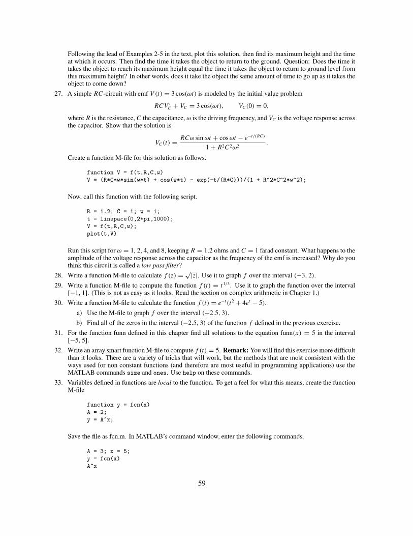
Following the lead of Examples 2-5 in the text, plot this solution, then find its maximum height and the timeat which it occurs. Then find the time it takes the object to return to the ground. Question: Does the time ittakes the object to reach its maximum height equal the time it takes the object to return to ground level fromthis maximum height? In other words, does it take the object the same amount of time to go up as it takes theobject to come down?

27. A simple RC-circuit with emf V (t) = 3 cos(ωt) is modeled by the initial value problem

RCV ′C + VC = 3 cos(ωt), VC(0) = 0,

where R is the resistance, C the capacitance, ω is the driving frequency, and VC is the voltage response acrossthe capacitor. Show that the solution is

VC(t) = RCω sin ωt + cos ωt − e−t/(RC)

1 + R2C2ω2.

Create a function M-file for this solution as follows.

function V = f(t,R,C,w)

V = (R*C*w*sin(w*t) + cos(w*t) - exp(-t/(R*C)))/(1 + R^2*C^2*w^2);

Now, call this function with the following script.

R = 1.2; C = 1; w = 1;

t = linspace(0,2*pi,1000);

V = f(t,R,C,w);

plot(t,V)

Run this script for ω = 1, 2, 4, and 8, keeping R = 1.2 ohms and C = 1 farad constant. What happens to theamplitude of the voltage response across the capacitor as the frequency of the emf is increased? Why do youthink this circuit is called a low pass filter?

28. Write a function M-file to calculate f (z) = √|z|. Use it to graph f over the interval (−3, 2).

29. Write a function M-file to compute the function f (t) = t1/3. Use it to graph the function over the interval[−1, 1]. (This is not as easy as it looks. Read the section on complex arithmetic in Chapter 1.)

30. Write a function M-file to calculate the function f (t) = e−t (t2 + 4et − 5).

a) Use the M-file to graph f over the interval (−2.5, 3).

b) Find all of the zeros in the interval (−2.5, 3) of the function f defined in the previous exercise.

31. For the function funn defined in this chapter find all solutions to the equation funn(x) = 5 in the interval[−5, 5].

32. Write an array smart function M-file to compute f (t) = 5. Remark: You will find this exercise more difficultthan it looks. There are a variety of tricks that will work, but the methods that are most consistent with theways used for non constant functions (and therefore are most useful in programming applications) use theMATLAB commands size and ones. Use help on these commands.

33. Variables defined in functions are local to the function. To get a feel for what this means, create the functionM-file

function y = fcn(x)

A = 2;

y = A^x;

Save the file as fcn.m. In MATLAB’s command window, enter the following commands.

A = 3; x = 5;

y = fcn(x)

A^x

59

Explain the discrepancy between the last two outputs. What is the current value of A in MATLAB’s workspace?

34. You can make variables global, allowing functions access to the variables in MATLAB’s workspace. To geta feel for what this means, create the function M-file

function y = gcn(x)

global A

A = 2;

y = A^x;

Save the file as gcn.m. In MATLAB’s command window, enter the following commands.

global A

A = 3; x = 5;

y = gcn(x)

A^x

Why are these last two outputs identical? What is the current value of A in MATLAB’s workspace?

60

5. Numerical Methods for ODEs

Numerical methods for solving ordinary differential equations are discussed in many textbooks.Here we will discuss how to use some of them in MATLAB. In particular, we will examine how areduction in the “step size” used by a particular algorithm reduces the error of the numerical solution,but only at a cost of increased computation time. In line with the philosophy that we are not emphasizingprogramming in this manual, MATLAB routines for these numerical methods are made available.

Our discussions of numerical methods will be very brief and incomplete. The assumption is thatthe reader is using a textbook in which these methods are described in more detail.

Euler’s Method

We want to find an approximate solution to the initial value problem y′ = f (t, y), with y(a) = y0,on the interval [a, b]. In Euler’s very geometric method, we go along the tangent line to the graph of thesolution to find the next approximation. We start by setting t0 = a and choosing a step size h. Then weinductively define

yk+1 = yk + hf (tk, yk),

tk+1 = tk + h,(5.1)

for k = 0, 1, 2, . . . , N , where N is large enough so that tN ≥ b. This algorithm is available in theMATLAB command eul1.

Example 1. Use Euler’s method to plot the solution of the initial value problem

y′ = y + t, y(0) = 1, (5.2)

on the interval [0, 3] .

Note that the differential equation in (5.2) is in normal form y′ = f (t, y), where f (t, y) = y + t .Before invoking the eul routine, you must first write a function M-file

function yprime = yplust(t,y)yprime = y + t;

to compute the right-hand side f (t, y) = y + t . Save the function M-file with the name yplust.m.Before continuing, it is always wise to test that your function M-file is returning the proper output. Forexample, f (1, 2) = 2 + 1, or 3, and

>> yplust(1,2)ans = 3

1 The function eul, as well as rk2 and rk4 described later in this chapter, are function M-files whichare not distributed with MATLAB. For example, type help eul to see if eul is installed correctly onyour computer. If not, see the Appendix to Chapter 3 for instructions on how to obtain them. The M-filesdefining these commands are printed in the appendix to this chapter for the illumination of the reader.

61

If you don’t receive this output, check your function yplust for coding errors. If all looks well, and youstill aren’t getting the proper output, refer to the section headed The MATLAB Path in Chapter 4.

Now that your function M-file is operational, it’s time to invoke the eul routine. The general syntaxis

[t,y]=eul(@yplust,tspan,y0,stepsize)

where yplust is the name of the function M-file, tspan is the vector [t0,tfinal] containing the initialand final time conditions, y0 is the y-value of the initial condition, and stepsize is the step size to beused in Euler’s method.2 Actually, the step size is an optional parameter. If you enter

[t,y]=eul(@yplust,tspan,y0)

the program will choose a default step size equal to (tfinal-t0)/100.

It is also possible to invoke eulwith the command [t,y]=eul('yplust',tspan,y0,stepsize).The only difference is the use of 'yplust' instead of @yplust. If you are using a version of MATLABprior to version 6, you have no choice. You must use 'yplust'. With version 6 you are given thechoice. Using the function handle @yplust will result in speedier solution. This speedup is not at allimportant for the simple equations we solve in this chapter. However, it becomes very important whenyou are solving more complicated systems of ODEs. The use of function handles also provides us withmore flexibility of use, as we will explain in Chapter 7. We will systematically use the function handlenotation, leaving it to you to make the replacement, if necessary.

The following commands will produce an approximate solution of the initial value problem (5.2)similar to that shown in Figure 5.1.

>> [t,y] = eul(@yplust,[0,3],1,1);>> plot(t,y,'.-')

We can arrange the output in two columns with the command

>> [t,y]ans =

0 11 22 53 12

Notice that the tk’s given in the first column differ by 1, the stepsize. The yk’s computed inductively bythe algorithm in (5.1) are in the second column. In Figure 5.1 these four points are plotted and connectedwith straight lines.

2 You can use an inline function defined with the command f = inline(’y+t’,’t’,’y’); insteadof the function M-file. Then the syntax for using eul is [t,y] = eul(f,tspan,y0,stepsize).

62

0 0.5 1 1.5 2 2.5 30

2

4

6

8

10

12

0 0.5 1 1.5 2 2.5 30

5

10

15

20

25

30

35

40

ExactEuler

Figure 5.1. Euler’s solution of initial valueproblem (5.1).

Figure 5.2. Euler versus exact solution(Step size h = 0.3).

Euler’s Method Versus the Exact Solution

In this section we want to examine visually the error in the numerical solution obtained from Euler’smethod.

Example 2. Re-examine the initial value problem

y′ = y + t, y(0) = 1. (5.3)

Compare the exact solution and the numerical solution obtained from Euler’s method on the interval[0, 3]. Use a step size of h = 0.3.

The initial value problem in (5.3) is linear and easily solved:

y = −t − 1 + 2et . (5.4)

The Euler’s method solution of the initial value problem in (5.3) with step size 0.3 is found by

>> h = 0.3;>> [teuler,yeuler] = eul(@yplust,[0,3],1,h);

We compute the exact solution using equation (5.4), but we want to choose a finer time increment on theinterval [0, 3] so that the exact solution will have the appearance of a smooth curve.

>> t = 0:.05:3;>> y = -t - 1 + 2*exp(t);

The command

>> plot(t,y,teuler,yeuler,'.')>> legend('Exact','Euler')

produces Figure 5.2, a visual image of the accuracy of Euler’s method using the step size h = 0.3 Theaccuracy is not too good in this case.

63

Changing the Step Size — Using Script M-Files

We would like to repeat the process in Example 2 with different step sizes to analyze graphicallyhow step size affects the accuracy of the approximation.

Example 3. Examine the numerical solutions provided by Euler’s method for the initial value problem

y′ = y + t, y(0) = 1,

on the interval [0, 3]. Use step sizes h = 0.2, 0.1, 0.05, and 0.025.

It will quickly get tedious to type the required commands into the Command Window. This is agood place to use a script M-file, as discussed in Chapter 2. We collect all of the commands and typethem once into an editor. To be precise, this file should contain the lines

[teuler,yeuler] = eul(@yplust,[0,3],1,h);t = 0:.05:3;y = -t - 1 + 2*exp(t);plot(t,y,teuler,yeuler,'.')legend('Exact','Euler')shg

We save the file as batch1.m (or whatever else we want to call it as long as it meets the requirementsfor function names). Then executing >> h = 0.2; batch1 produces Figure 5.3, while the command>> h = 0.05; batch1 produces Figure 5.5.

0 0.5 1 1.5 2 2.5 30

5

10

15

20

25

30

35

40ExactEuler

0 0.5 1 1.5 2 2.5 30

5

10

15

20

25

30

35

40ExactEuler

Figure 5.3. Euler versus exact solution(Step size h = 0.2).

Figure 5.4. Euler versus exact solution(Step size h = 0.05).

Repeating this command with various values of the step size h allows us to visually examine theeffect of choosing smaller and smaller step sizes. Note how the error decreases, but the computation timeincreases as you reduce the step size.

64

Numerical Error Analysis

In this section we analyze the error inherent in Euler’s method numerically as well as graphicallyby computing the absolute error at each step, defined as the absolute value of the difference between theactual solution and the numerical solution at that step. We will continue to look at the error graphically.

Example 4. Consider again the initial value problem

y′ = y + t, y(0) = 1,

on the interval [0, 3]. Record the maximum error in the Euler’s solution for the step sizes h =0.2, 0.1, 0.05, and 0.025.

We record the error at each step by adjusting the script file batch1.m from Example 3. We need toevaluate the exact solution at the same points at which we have the approximate values calculated, i.e. atthe points in the vector teuler. This is easy. Simply enter z = -teuler - 1 + 2*exp(teuler). Thento compare with the approximate values, we look at the difference of the two vectors z and yeuler. Weare only interested in the magnitude of the error and not the sign. The command abs(z-yeuler) yieldsa vector containing the absolute value of the error made at each step of the Euler computation. Finally, wecompute the largest of these errors with the MATLAB command maxerror = max(abs(z-yeuler)).We enter this command without an ending semi-colon, because we want to see the result in the commandwindow. Therefore, to effect these changes we alter the file batch1.m to

[teuler,yeuler] = eul(@yplust,[0,3],1,h);t = 0:.05:3;y = -t - 1 + 2*exp(t);plot(t,y,teuler,yeuler,'.')legend('Exact','Euler')shgz = -teuler - 1 + 2*exp(teuler);maxerror = max(abs(z - yeuler))

Save this file as batch2.m. A typical session might show the following in the command window:

>> h = 0.2; batch2maxerror =

9.3570>> h = 0.1; batch2maxerror =

5.2723>> h = 0.05; batch2maxerror =

2.8127

Of course, each of these commands will result in a visual display of the error in the figure window aswell. Thus, we can very easily examine the error in Euler’s method both graphically and quantitatively.

If you have executed all of the commands up to now, you will have noticed that decreasing the stepsize has the effect of reducing the error. But at what expense? If you continue to execute batch2, halving

65

the step size each time, you will notice that the routine takes more and more time to complete. In fact,halving the step size doubles the number of computations that must take place and therefore doublesthe time needed. Therefore, decreasing the step size used in Euler’s method is expensive, in terms ofcomputer time. However, notice that halving the step size results in a maximum error almost exactly halfthe previous one.

At this point it would be illuminating to see a plot of how the maximum error changes versus thestep size.

Example 5. Consider again the initial value problem

y′ = y + t, y(0) = 1.

Sketch a graph of the maximum error in Euler’s method versus the step size.

To do this using MATLAB, we have to devise a way to capture the various step sizes and the associatederrors into vectors and then use an appropriate plotting command. We will call the vector of step sizesh_vect and the vector of errors err_vect. The following modification of batch2.m will do the job.Save the file as batch3.m

h_vect = []; err_vect = []; h = 1;t = 0:.05:3;y = -t - 1 + 2*exp(t);for k = 1:8

[teuler,yeuler] = eul(@yplust,[0,3],1,h);plot(t,y,teuler,yeuler,'.')legend('Exact','Euler',2)shgz = -teuler - 1 + 2*exp(teuler);maxerror = max(abs(z - yeuler));h_vect = [h_vect,h]err_vect = [err_vect,maxerror]pauseh = h/2;

end

The first line initializes h_vect, err_vect, and the starting step size h = 1. Since at the beginning theycontain no information, h_vect and err_vect are defined to be empty matrices, as indicated by [].The next two lines compute the exact solution for later plotting. The main work is done in the for loop.This comprises all of the indented steps between for k = 1:8 and end. The first four lines computethe approximate solution, and plot it in comparison with the exact solution. Notice the third input to thelegend command. This results in the legend being placed in the upper left corner, where it does notinterfere with the graph. The maximum error is computed next and the new step size and error are addedto the vectors h_vect and err_vect. The command pause stops the execution and gives you time toobserve the figure and the output in the command window. When you are finished examining the figureand output, hit any key (the space bar will do) to advance to the next step. The final line in the for loophalves the step size in preparation for the next step. Notice that the for loop is executed 8 times withdifferent values of k

66

Now we are ready to go. Executing batch3 results in a visual display similar to Figures 5.3 or 5.4at each step. There is also output on the command window because we have not ended the h_vect =... and err_vect = ... commands with semi-colons. By hitting a key twice, we get three steps ofthe for loop, and the output

>> batch3h_vect =

1err_vect =

24.1711h_vect =

1.0000 0.5000err_vect =

24.1711 17.3898h_vect =

1.0000 0.5000 0.2500err_vect =

24.1711 17.3898 11.0672

at the command line. Continuing to step through batch3, we get more and more data. After the seventhiteration the output is

h_vect =1.0000 0.5000 0.2500 0.1250 0.0625 0.0313 0.0156

err_vect =24.1711 17.3898 11.0672 6.3887 3.4581 1.8030 0.9211

Notice that the maximum error is approximately halved on each step, at least on the last few steps.

After all eight steps we are ready to plot the error data. This can be done with any of the commandsplot, semilogx, semilogy, or loglog. Try them all to see which you like best. However, since themaximum error seems to be halved each time the step size is halved, we expect a power law relationship.Therefore we will use a loglog graph. The commands

>> loglog(h_vect,err_vect)>> xlabel('Step size')>> ylabel('Maximum error')>> title('Maximum error vs. step size for Euler''s method')>> grid>> axis tight

produce Figure 5.5. The command axis tight sets the axis limits to the range of the data.

Notice that the graph of the logarithm of the maximum error versus the logarithm of the step sizeis approximately linear. If the graph were truly linear, we would have a linear relationship between thelogarithms of the coordinates, like

log10(maximum error) = A + B log10(step size),

67

10−2

10−1

100

100

101

Step size

Max

imum

err

or

Maximum error vs. step size for Euler’s method

Figure 5.5. Analysis of the error in Euler’s method.

for some constants A and B.3

If we exponentiate this relationship, we get

maximum error = 10A · (step size)B = C(step size)B,

where C = 10A. Thus a linear relationship with slope B on a loglog graph means that there is a powerlaw relationship between the coordinates with the exponent being B. Indeed, we will see in Exercise 21that Euler’s method is a first order method. This means that if yk is the calculated approximation at tk ,and y(tk) is the exact solution evaluated at tk , then |y(tk) − yk| is the error being made, and it satisfies aninequality of the form

|y(tk) − yk| ≤ C|h|, for all k, (5.5)

where C is a constant. This inequality satisfied by the error is reflected in the nearly linear relationshipwe see in Figure 5.5, and it is the reason why we chose a loglog graph.

Hopefully, you now understand two key points about Euler’s method. You can increase the accuracyof the solution by decreasing the step size, but you pay for the increase in accuracy with an increase inthe number of computational steps and therefore in the computing time.

The Second Order Runge-Kutta Method

What is needed are solution routines that will provide more accuracy without having to drasticallyreduce the step size and therefore increase the computation time. The Runge-Kutta routines are designedto do just that. The simplest of these, the Runge-Kutta method of order two, is sometimes called theimproved Euler’s method. Again, we want to find a approximate solution of the initial value problem

3 We are using the logarithm to base 10 instead of the natural logarithm because it is the basis ofthe loglog graph. However there is very little difference in this case. Since ln x = log10 x · ln 10, theinequality is true with log10 replaced by ln, with the same slope B and A replaced by A · ln 10.

68

y′ = f (t, y), with y(a) = y0, on the interval [a, b]. As before, we set t0 = a, choose a step size h, andthen inductively define

s1 = f (tk, yk),

s2 = f (tk + h, yk + hs1),

yk+1 = yk + h(s1 + s2)/2,

tk+1 = tk + h,

for k = 0, 1, 2, . . . , N , where N is large enough so that tN ≥ b. This algorithm is available in the M-filerk2.m, which is listed in the appendix of this chapter.

The syntax for using rk2 is exactly the same as the syntax used for eul. As the name indicates, itis a second order method, so, if yk is the calculated approximation at tk , and y(tk) is the exact solutionevaluated at tk , then there is a constant C such that

|y(tk) − yk| ≤ C|h|2, for all k. (5.6)

Notice that the error is bounded by a constant times the square of the step size. As we did for Euler’smethod, we have a power inequality, but now the power is 2 instead of 1. We should expect a nearlylinear relationship between the maximum error and the step size in a loglog graph, but with a steeperslope than we observed for Euler’s method.

The error in the second order Runge-Kutta method can be examined experimentally using the sametechniques that we illustrated for Euler’s method. Modify the script files, batch1.m, batch2.m, andbatch3.m, replacing the command eul with rk2 everywhere it occurs, and changing all references toeuler to refer to rk2 instead. You might also want to change the names of the files to indicate that theynow refer to rk2. Replay the commands in Examples 3, 4, and 5 using your newly modified routines.

The Fourth Order Runge-Kutta Method

This is the final method we want to consider. We want to find an approximate solution to the initialvalue problem y′ = f (t, y), with y(a) = y0, on the interval [a, b]. We set t0 = a and choose a step sizeh. Then we inductively define

s1 = f (tk, yk),

s2 = f (tk + h/2, yk + hs1/2),

s3 = f (tk + h/2, yk + hs2/2),

s4 = f (tk + h, yk + hs3),

yk+1 = yk + h(s1 + 2s2 + 2s3 + s4)/6,

tk+1 = tk + h,

for k = 0, 1, 2, . . . , N , where N is large enough so that tN ≥ b. This algorithm is available in the M-filerk4.m, which is listed in the appendix of this chapter.

The syntax for using rk4 is exactly the same as that required by eul or rk2. As the name indicates,it is a fourth order method, so, if yk is the calculated approximation at tk , and y(tk) is the exact solutionevaluated at tk , there is a constant C such that

|y(tk) − yk| ≤ C|h|4, for all k. (5.7)

69

The error in the fourth order Runge-Kutta method can be examined experimentally using the sametechniques that we illustrated for Euler’s and the Runge-Kutta 2 methods. Again, you can easily modifythe script files, batch1.m, batch2.m, and batch3.m to create files to evaluate the errors in the Runge-Kutta 4 algorithm. Since the error is bounded by a constant times the fourth power of the step size in(5.7), we again expect a nearly linear relationship between the maximum error and the step size in aloglog graph, but with a much steeper slope than before.

Comparing Euler, RK2, and RK4

It is very interesting to compare the accuracy of these three methods, both for individual step sizes,and for a range of step sizes.

Example 6. Consider again the initial value problem

y′ = y + t, y(0) = 1.

Sketch a graph of the maximum error in each of the three methods (Euler, RK2, RK4) versus the stepsize.

This can be done by writing a script M-file that is only a minor modification of batch3. Create ascript M-file with the contents

h = 1; eul_vect = []; rk2_vect = []; rk4_vect = []; h_vect=[];t = 0:.05:3;y = -t - 1 + 2*exp(t);for k=1:8

[teuler,yeuler] = eul(@yplust,[0,3],1,h);[trk2,yrk2] = rk2(@yplust,[0,3],1,h);[trk4,yrk4] = rk4(@yplust,[0,3],1,h);plot(t,y,teuler,yeuler,'.',trk2,yrk2,'+',trk4,yrk4,'x')legend('Exact','Euler','RK2','RK4',2)shgzeuler = -teuler - 1 + 2*exp(teuler);eulerror = max(abs(zeuler - yeuler));zrk2 = -trk2 - 1 + 2*exp(trk2);rk2error = max(abs(zrk2 - yrk2));zrk4 = -trk4 - 1 + 2*exp(trk4);rk4error = max(abs(zrk4 - yrk4));h_vect = [h_vect,h]eul_vect = [eul_vect,eulerror]rk2_vect = [rk2_vect,rk2error]rk4_vect = [rk4_vect,rk4error]pauseh = h/2;

endloglog(h_vect,eul_vect,h_vect,rk2_vect,h_vect,rk4_vect)legend('eul','rk2','rk4',4)grid, xlabel('Step size'), ylabel('Maximum error')title('Maximum error vs. step size'), axis tight

70

Save the file as batch4.m.

Most of the features of batch4 are already present in batch3. The major difference is that we haveadded the plot commands for the loglog graph at the end, so that it will automatically be executed whenthe error data has been computed. Executing all eight steps in batch4 will result in a plot of the errorcurves for each of the three methods, as shown in Figure 5.6.4

10−2

10−1

100

10−8

10−6

10−4

10−2

100

Step size

Max

imum

err

orMaximum error vs. step size

eulrk2rk4

Figure 5.6. Error comparison for Euler, RK2, and RK4.

Note that Euler’s method has the largest error for a given step size, with Runge-Kutta 2 being slightlybetter, while Runge-Kutta 4 is significantly better than the other two. Also notice that the curves are nearlystraight lines in the loglog plot in Figure 5.6, indicating a power function relationship between the errorand and the stepsize, as predicted by the inequalities (5.5), (5.6), and (5.7). The slopes of the curves arealso roughly comparable to the order of the corresponding method. (Exercises 13–20 demonstrate therelation between a power function and its loglog plot. Exercise 21 experimentally determines the ordersof the methods eul, rk2, and rk4)

Exercises

In Exercises 1–6 perform the following tasks for the given initial value problem on the specified interval.

a) Find the exact solution.

b) Use MATLAB to plot on a single figure window the graph of the exact solution, together with the plotsof the solutions using each of the three methods (eul, rk2, and rk4) with the given step size h. Usea distinctive marker (type help plot for help on available markers) for each method. Label the graphappropriately and add a legend to the plot.

4 As you execute batch4.m repeatedly, you will note that the vector rk4 vect appears to have zeroentries except for the first two. Is the error from rk4 actually zero at this point? The answer is no. Tosee what the entries really are we need to print the vector with more accuracy. To do this, enter formatlong and then rk4 vect to see what you get.

71

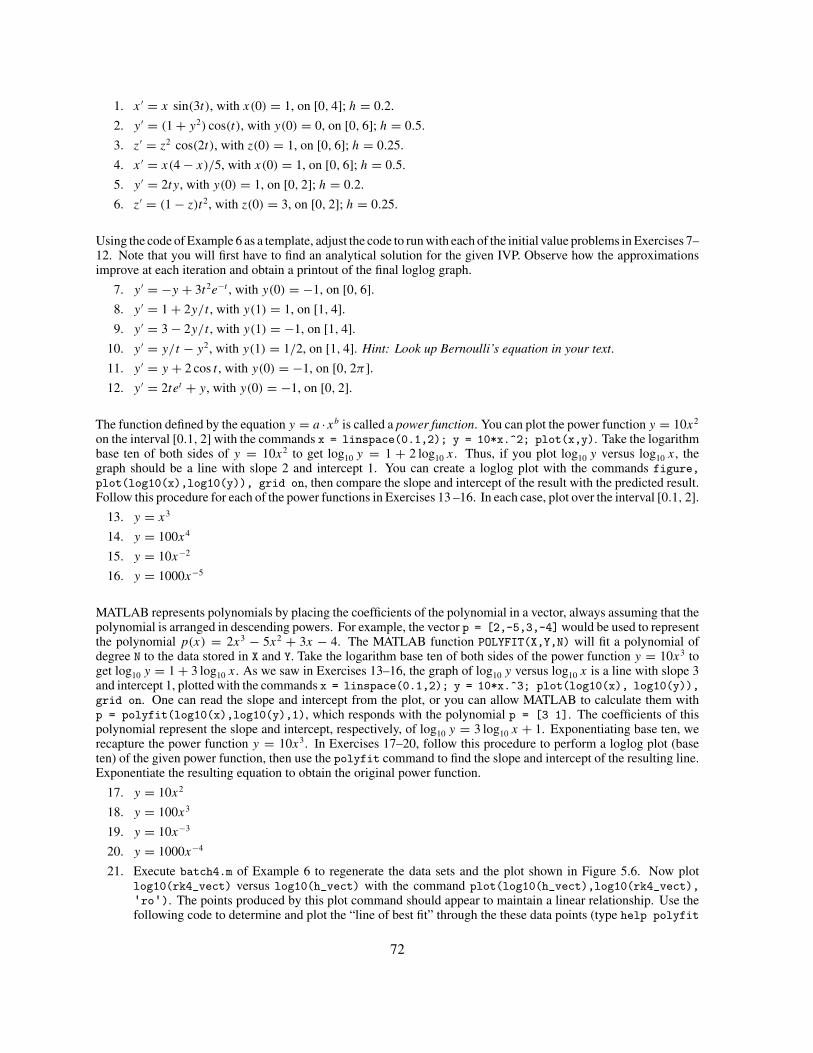
1. x ′ = x sin(3t), with x(0) = 1, on [0, 4]; h = 0.2.

2. y ′ = (1 + y2) cos(t), with y(0) = 0, on [0, 6]; h = 0.5.

3. z′ = z2 cos(2t), with z(0) = 1, on [0, 6]; h = 0.25.

4. x ′ = x(4 − x)/5, with x(0) = 1, on [0, 6]; h = 0.5.

5. y ′ = 2ty, with y(0) = 1, on [0, 2]; h = 0.2.

6. z′ = (1 − z)t2, with z(0) = 3, on [0, 2]; h = 0.25.

Using the code of Example 6 as a template, adjust the code to run with each of the initial value problems in Exercises 7–12. Note that you will first have to find an analytical solution for the given IVP. Observe how the approximationsimprove at each iteration and obtain a printout of the final loglog graph.

7. y ′ = −y + 3t2e−t , with y(0) = −1, on [0, 6].

8. y ′ = 1 + 2y/t , with y(1) = 1, on [1, 4].

9. y ′ = 3 − 2y/t , with y(1) = −1, on [1, 4].

10. y ′ = y/t − y2, with y(1) = 1/2, on [1, 4]. Hint: Look up Bernoulli’s equation in your text.

11. y ′ = y + 2 cos t , with y(0) = −1, on [0, 2π ].

12. y ′ = 2tet + y, with y(0) = −1, on [0, 2].

The function defined by the equation y = a ·xb is called a power function. You can plot the power function y = 10x2

on the interval [0.1, 2] with the commands x = linspace(0.1,2); y = 10*x.^2; plot(x,y). Take the logarithmbase ten of both sides of y = 10x2 to get log10 y = 1 + 2 log10 x. Thus, if you plot log10 y versus log10 x, thegraph should be a line with slope 2 and intercept 1. You can create a loglog plot with the commands figure,

plot(log10(x),log10(y)), grid on, then compare the slope and intercept of the result with the predicted result.Follow this procedure for each of the power functions in Exercises 13 –16. In each case, plot over the interval [0.1, 2].

13. y = x3

14. y = 100x4

15. y = 10x−2

16. y = 1000x−5

MATLAB represents polynomials by placing the coefficients of the polynomial in a vector, always assuming that thepolynomial is arranged in descending powers. For example, the vector p = [2,-5,3,-4] would be used to representthe polynomial p(x) = 2x3 − 5x2 + 3x − 4. The MATLAB function POLYFIT(X,Y,N) will fit a polynomial ofdegree N to the data stored in X and Y. Take the logarithm base ten of both sides of the power function y = 10x3 toget log10 y = 1 + 3 log10 x. As we saw in Exercises 13–16, the graph of log10 y versus log10 x is a line with slope 3and intercept 1, plotted with the commands x = linspace(0.1,2); y = 10*x.^3; plot(log10(x), log10(y)),

grid on. One can read the slope and intercept from the plot, or you can allow MATLAB to calculate them withp = polyfit(log10(x),log10(y),1), which responds with the polynomial p = [3 1]. The coefficients of thispolynomial represent the slope and intercept, respectively, of log10 y = 3 log10 x + 1. Exponentiating base ten, werecapture the power function y = 10x3. In Exercises 17–20, follow this procedure to perform a loglog plot (baseten) of the given power function, then use the polyfit command to find the slope and intercept of the resulting line.Exponentiate the resulting equation to obtain the original power function.

17. y = 10x2

18. y = 100x3

19. y = 10x−3

20. y = 1000x−4

21. Execute batch4.m of Example 6 to regenerate the data sets and the plot shown in Figure 5.6. Now plotlog10(rk4_vect) versus log10(h_vect) with the command plot(log10(h_vect),log10(rk4_vect),

'ro'). The points produced by this plot command should appear to maintain a linear relationship. Use thefollowing code to determine and plot the “line of best fit” through the these data points (type help polyfit

72

and help polyval to get a full explanation of these commands).

hold on %hold the prior plot

p = polyfit(log10(h_vect),log10(rk4_vect),1)

plot(log10(h_vect),polyval(p,log10(h_vect)),'g')

Write the equation of the line of best fit in the form log10(rk4 vect) = C log10(h vect) + B, where C andB are the slope and intercept captured from the polyfit command. Solve this last equation for rk4_vect.How closely does this last equation compare with the inequality (5.7)?

a) Perform a similar analysis on eul_vect and h_vect and compare with the inequality (5.5).

b) Perform a similar analysis on rk2_vect and h_vect and compare with the inequality (5.6).

22. Simple substitution will reveal that x(t) = π/2 is a solution of x ′ = et cos x. Moreover, both f (t, x) =et cos x and ∂f/∂x = −et sin x are continuous everywhere. Therefore, solutions are unique and no twosolutions can ever share a common point (solutions cannot intersect). Use Euler’s method with a step size h =0.1 to plot the solution of x ′ = et cos x with initial condition x(0) = 1 on the interval [0, 2π ] and hold the graph(hold on). Overlay the graph of x = π/2 with the command line([0,2*pi],[pi/2,pi/2],'color','r')and note that the solutions intersect. Does reducing the step size help? If so, does this reduced step size holdup if you increase the interval to [0, 10]? How do rk2 and rk4 perform on this same problem?

23. The accuracy of any numerical method in solving a differential equation y ′ = f (t, y) depends on how stronglythe equation depends on the variable y. More precisely, the constants that appear in the error bounds dependon the derivatives of f with respect to y. To see this experimentally, consider the two initial value problems

y ′ = y, y(0) = 1,

y ′ = et , y(0) = 1.

You will notice that the two problems have the same solution. For each of the three methods described inthis chapter compute approximate solutions to these two initial value problems over the interval [0, 1] usinga step size of h = 0.01. For each method compare the accuracy of the solution to the two problems.

24. Remember that y(t) = et is the solution to the initial value problem y ′ = y, y(0) = 1. Then e = e1, andin MATLAB this is e = exp(1). Suppose we try to calculate e approximately by solving the initial valueproblem, using the methods of this chapter. Use step sizes of the form 1/n, where n is an integer. For each ofEuler’s method, the second order Runge-Kutta method, and the fourth order Runge-Kutta method, how largedoes n have to be to get an approximation eapp which satisfies |eapp − e| ≤ 10−3?

25. In the previous problem, show that the approximation to e using Euler’s method with step size 1/n is (1+1/n)n.As a challenge problem, compute the formulas for the approximations using the two Runge-Kutta methods.

Appendix: M-files for Numerical Methods

In this appendix we provide a listing of the programs eul.m, rk2.m, and rk4.m used in the chapter. The firstlisting is the file eul.m.

function [tout, yout] = eul(FunFcn, tspan, y0, ssize)

%

% EUL Integrates a system of ordinary differential equations using

% Euler's method. See also ODE45 and ODEDEMO.

% [t,y] = eul('yprime', tspan, y0) integrates the system

% of ordinary differential equations described by the M-file

% yprime.m over the interval tspan = [t0,tfinal] and using initial

% conditions y0.

% [t, y] = eul(F, tspan, y0, ssize) uses step size ssize

73

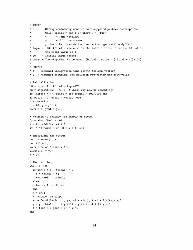
% INPUT:

% F - String containing name of user-supplied problem description.

% Call: yprime = fun(t,y) where F = 'fun'.% t - Time (scalar).

% y - Solution vector.

% yprime - Returned derivative vector; yprime(i) = dy(i)/dt.

% tspan = [t0, tfinal], where t0 is the initial value of t, and tfinal is

% the final value of t.

% y0 - Initial value vector.

% ssize - The step size to be used. (Default: ssize = (tfinal - t0)/100).

%

% OUTPUT:

% t - Returned integration time points (column-vector).

% y - Returned solution, one solution row-vector per tout-value.

% Initialization

t0 = tspan(1); tfinal = tspan(2);

pm = sign(tfinal - t0); % Which way are we computing?

if (nargin < 4), ssize = abs(tfinal - t0)/100; end

if ssize < 0, ssize = -ssize; end

h = pm*ssize;

t = t0; y = y0(:);

tout = t; yout = y.';

% We need to compute the number of steps.

dt = abs(tfinal - t0);

N = floor(dt/ssize) + 1;

if (N-1)*ssize < dt, N = N + 1; end

% Initialize the output.

tout = zeros(N,1);

tout(1) = t;

yout = zeros(N,size(y,1));

yout(1,:) = y.';k = 1;

% The main loop

while k < N

if pm*(t + h - tfinal) > 0

h = tfinal - t;

tout(k+1) = tfinal;

else

tout(k+1) = t0 +k*h;

end

k = k+1;

% Compute the slope

s1 = feval(FunFcn, t, y); s1 = s1(:); % s1 = f(t(k),y(k))

y = y + h*s1; % y(k+1) = y(k) + h*f(t(k),y(k))

t = tout(k); yout(k,:) = y.';end;

74

Since we are not teaching programming, we will not explain everything in this file, but a few things should beexplained. The % is MATLAB’s symbol for comments. MATLAB ignores everything that appears on a line aftera %. The large section of comments that appears at the beginning of the file can be read using the MATLAB help

command. Enter help eul and see what happens. Notice that these comments at the beginning take up more thanhalf of the file. That’s an indication of how easy it is to program these algorithms. In addition, a couple of lines ofthe code are needed only to allow the program to handle systems of equations.

Next, we present the M-file for the second order Runge-Kutta method, without the help file, which is prettymuch identical to the help file in eul.m. You can type help rk2 to view the help file in MATLAB’s commandwindow.

function [tout, yout] = rk2(FunFcn, tspan, y0, ssize)

% Initialization

t0 = tspan(1);

tfinal = tspan(2);

pm = sign(tfinal - t0); % Which way are we computing?

if nargin < 4, ssize = (tfinal - t0)/100; end

if ssize < 0, ssize = -ssize; end

h = pm*ssize;

t = t0;

y = y0(:);

% We need to compute the number of steps.

dt = abs(tfinal - t0);

N = floor(dt/ssize) + 1;

if (N-1)*ssize < dt

N = N + 1;

end

% Initialize the output.

tout = zeros(N,1);

tout(1) = t;

yout = zeros(N,size(y,1));

yout(1,:) = y.';k = 1;

% The main loop

while k < N

if pm*(t + h - tfinal) > 0

h = tfinal - t;

tout(k+1) = tfinal;

else

tout(k+1) = t0 +k*h;

end

k = k + 1;

s1 = feval(FunFcn, t, y); s1 = s1(:);

s2 = feval(FunFcn, t + h, y + h*s1); s2 = s2(:);

y = y + h*(s1 + s2)/2; t = tout(k);

yout(k,:) = y.';end;

75

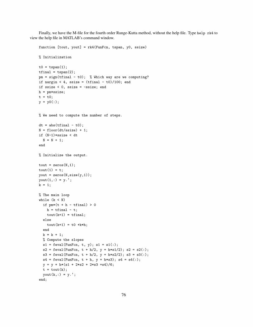
Finally, we have the M-file for the fourth order Runge-Kutta method, without the help file. Type help rk4 toview the help file in MATLAB’s command window.

function [tout, yout] = rk4(FunFcn, tspan, y0, ssize)

% Initialization

t0 = tspan(1);

tfinal = tspan(2);

pm = sign(tfinal - t0); % Which way are we computing?

if nargin < 4, ssize = (tfinal - t0)/100; end

if ssize < 0, ssize = -ssize; end

h = pm*ssize;

t = t0;

y = y0(:);

% We need to compute the number of steps.

dt = abs(tfinal - t0);

N = floor(dt/ssize) + 1;

if (N-1)*ssize < dt

N = N + 1;

end

% Initialize the output.

tout = zeros(N,1);

tout(1) = t;

yout = zeros(N,size(y,1));

yout(1,:) = y.';k = 1;

% The main loop

while (k < N)

if pm*(t + h - tfinal) > 0

h = tfinal - t;

tout(k+1) = tfinal;

else

tout(k+1) = t0 +k*h;

end

k = k + 1;

% Compute the slopes

s1 = feval(FunFcn, t, y); s1 = s1(:);

s2 = feval(FunFcn, t + h/2, y + h*s1/2); s2 = s2(:);

s3 = feval(FunFcn, t + h/2, y + h*s2/2); s3 = s3(:);

s4 = feval(FunFcn, t + h, y + h*s3); s4 = s4(:);

y = y + h*(s1 + 2*s2 + 2*s3 +s4)/6;

t = tout(k);

yout(k,:) = y.';end;

76

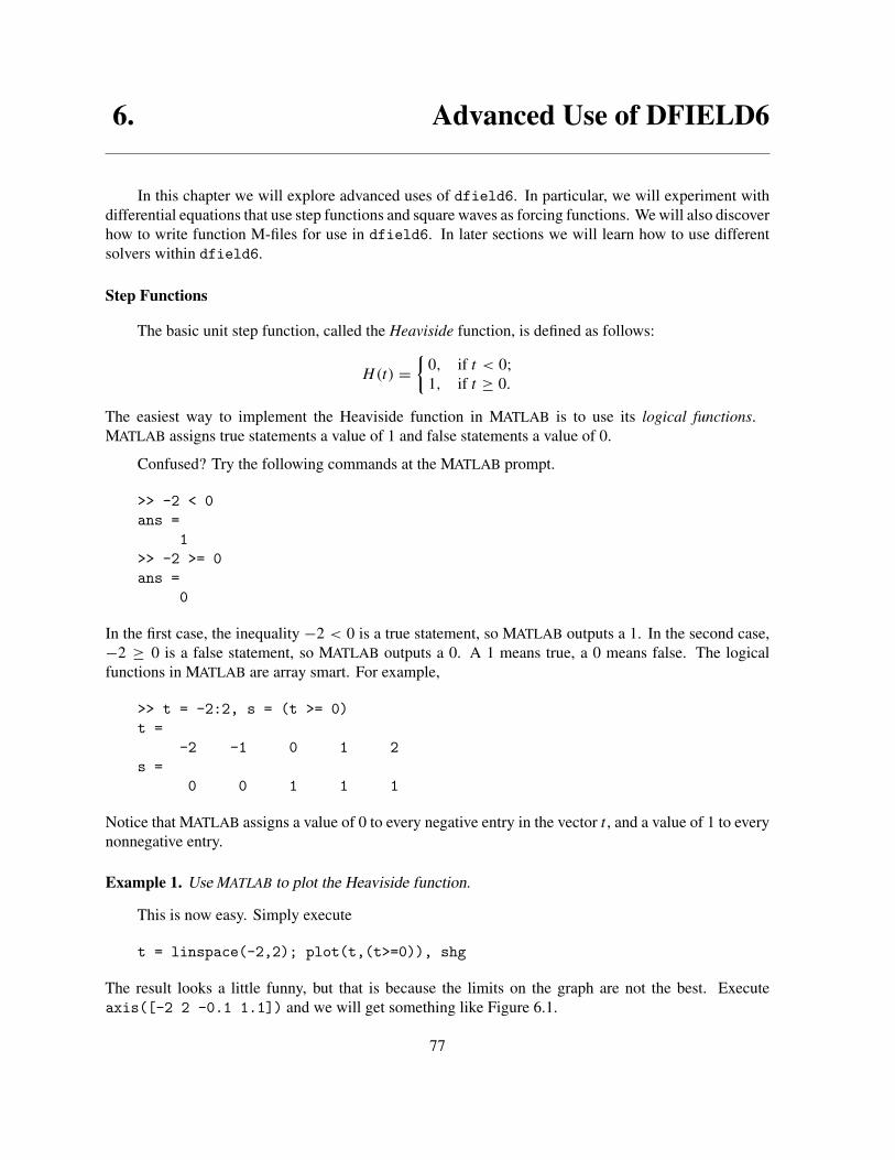
6. Advanced Use of DFIELD6

In this chapter we will explore advanced uses of dfield6. In particular, we will experiment withdifferential equations that use step functions and square waves as forcing functions. We will also discoverhow to write function M-files for use in dfield6. In later sections we will learn how to use differentsolvers within dfield6.

Step Functions

The basic unit step function, called the Heaviside function, is defined as follows:

H(t) ={

0, if t < 0;1, if t ≥ 0.

The easiest way to implement the Heaviside function in MATLAB is to use its logical functions.MATLAB assigns true statements a value of 1 and false statements a value of 0.

Confused? Try the following commands at the MATLAB prompt.

>> -2 < 0ans =

1>> -2 >= 0ans =

0

In the first case, the inequality −2 < 0 is a true statement, so MATLAB outputs a 1. In the second case,−2 ≥ 0 is a false statement, so MATLAB outputs a 0. A 1 means true, a 0 means false. The logicalfunctions in MATLAB are array smart. For example,

>> t = -2:2, s = (t >= 0)t =

-2 -1 0 1 2s =

0 0 1 1 1

Notice that MATLAB assigns a value of 0 to every negative entry in the vector t , and a value of 1 to everynonnegative entry.

Example 1. Use MATLAB to plot the Heaviside function.

This is now easy. Simply execute

t = linspace(-2,2); plot(t,(t>=0)), shg

The result looks a little funny, but that is because the limits on the graph are not the best. Executeaxis([-2 2 -0.1 1.1]) and we will get something like Figure 6.1.

77

The Heaviside function is a “discontinuous” function, so the almost vertical line connecting thetwo constant portions of the graph in Figure 6.1 should not be present. It is present only because theMATLAB linestyle we selected connects consecutive points of the plot with line segments. If we replacedthe linspace command with linspace(-2,2,1000), the almost vertical portion would look trulyvertical. It still should not be there, but we will put up with it.

The logical functions are particularly handy when a problem calls for the use of a piecewise function,a function that is defined in two or more pieces.

Example 2. Sketch the graph of the piecewise defined function

f (t) ={

t, if t < 1;1, if t ≥ 1;

(6.1)

on the interval [0, 2].

−2 −1.5 −1 −0.5 0 0.5 1 1.5 2

0

0.2

0.4

0.6

0.8

1

H(t

)

t

0 0.2 0.4 0.6 0.8 1 1.2 1.4 1.6 1.8 20

0.1

0.2

0.3

0.4

0.5

0.6

0.7

0.8

0.9

1

y =

f(t)

t

Figure 6.1. The Heaviside function. Figure 6.2. The plot of f in (6.1).

Consider the following pseudocode, where we incorporate the use of MATLAB’s logical functions,

g(t) = t · (t < 1) + 1 · (t ≥ 1).

If t < 1, then t < 1 is a true statement and evaluates to 1, but t ≥ 1 is a false statement and evaluates to0. Consequently, if t < 1,

g(t) = t · (t < 1) + 1 · (t ≥ 1) = t · (1) + 1 · (0) = t.

However, if t ≥ 1, then t < 1 is false and evaluates to 0, but t ≥ 1 is now a true statement and evaluatesto 1. Consequently, if t ≥ 1,

g(t) = t · (t < 1) + 1 · (t ≥ 1) = t · (0) + 1 · (1) = 1.

Note that these results agree with the definition of f (t) in equation (6.1). Consequently, f (t) = g(t)

for all values of t and we can use f (t) = t · (t < 1) + 1 · (t ≥ 1) to sketch the graph of the piecewisefunction f (t).

78

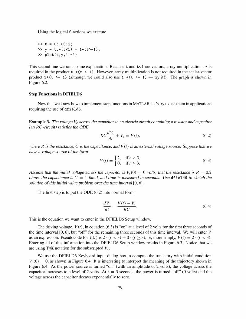
Using the logical functions we execute

>> t = 0:.05:2;>> y = t.*(t<1) + 1*(t>=1);>> plot(t,y,'.-')

This second line warrants some explanation. Because t and t<1 are vectors, array multiplication .* isrequired in the product t.*(t < 1). However, array multiplication is not required in the scalar-vectorproduct 1*(t >= 1) (although we could also use 1.*(t >= 1) — try it!). The graph is shown inFigure 6.2.

Step Functions in DFIELD6

Now that we know how to implement step functions in MATLAB, let’s try to use them in applicationsrequiring the use of dfield6.

Example 3. The voltage Vc across the capacitor in an electric circuit containing a resistor and capacitor(an RC-circuit) satisfies the ODE

RCdVc

dt+ Vc = V (t), (6.2)

where R is the resistance, C is the capacitance, and V (t) is an external voltage source. Suppose that wehave a voltage source of the form

V (t) ={

2, if t < 3;0, if t ≥ 3.

(6.3)

Assume that the initial voltage across the capacitor is Vc(0) = 0 volts, that the resistance is R = 0.2ohms, the capacitance is C = 1 farad, and time is measured in seconds. Use dfield6 to sketch thesolution of this initial value problem over the time interval [0, 6].

The first step is to put the ODE (6.2) into normal form,

dVc

dt= V (t) − Vc

RC. (6.4)

This is the equation we want to enter in the DFIELD6 Setup window.

The driving voltage, V (t), in equation (6.3) is “on” at a level of 2 volts for the first three seconds ofthe time interval [0, 6], but “off” for the remaining three seconds of this time interval. We will enter V

as an expression. Pseudocode for V (t) is 2 · (t < 3) + 0 · (t ≥ 3), or, more simply, V (t) = 2 · (t < 3).Entering all of this information into the DFIELD6 Setup window results in Figure 6.3. Notice that weare using TEX notation for the subscripted Vc.

We use the DFIELD6 Keyboard input dialog box to compute the trajectory with initial conditionVc(0) = 0, as shown in Figure 6.4. It is interesting to interpret the meaning of the trajectory shown inFigure 6.4. As the power source is turned “on” (with an amplitude of 2 volts), the voltage across thecapacitor increases to a level of 2 volts. At t = 3 seconds, the power is turned “off” (0 volts) and thevoltage across the capacitor decays exponentially to zero.

79

Figure 6.3. Setting up the circuit equation.

0 1 2 3 4 5 6

0

0.5

1

1.5

2

2.5

3

3.5

4

t

Vc

Vc ’ = (V − V

c)/(R C) R = 0.2 C = 1 V = 2 (t<3)

Figure 6.4. Solution trajectory with initial condition Vc(0) = 0.

Using Function M-files in DFIELD6

Let’s look at another example that exhibits new features of dfield6.

Example 4. Suppose that originally there are 10 tons of fish in a lake. The fish population is governedby the logistic equation with a natural reproductive rate of r = 1 and a carrying capacity of K = 10.

Starting at t = 0, the fish are harvested at the rate of 3 tons per month for the first three months and 0.5tons per month after that. Use dfield6 to sketch the population over 18 months.

We will use tons as the units for P and months for t . Then the population P(t) satisfies the equation

dP

dt= rP

(

1 − P

K

)

− H, (6.5)

where the harvesting function H is defined by

H(t) ={

3, if t ≤ 3,0.5, if t > 3.

(6.6)

80

Note that the harvesting strategy in equation (6.6) exhibits heavy harvesting for the first three months (3tons per month), while the harvesting is lighter in the remaining months (0.5 tons per month).

We could handle this problem using the same method we used in Example 3, by entering the right-hand side of equation (6.5) in the DFIELD6 Setup window, and then using the pseudocode H(t) =3 · (t ≤ 3) + 0.5 · (t > 3) to define the expression H. However, we want to use this example to illustratethe use of function M-files in dfield6.

Start by opening your editor and creating a function M-file with the following code.

function H = harvest(t)if t <= 3

H = 3;else

H = 0.5;end

At first glance this looks like the perfect M-file for our harvesting function H(t). However, functionM-files used in dfield6 must be array smart, and the function harvest is not. We can see this by testingit, say on the vector 0:6. To make harvest array smart, we use the fact that the function is piecewisedefined and use the logical functions as we have been doing. A correct version is

function H = harvest(t)H = 3*(t <= 3) + 0.5*(t > 3);

Now we get

>> harvest(0:6)ans =

3.0000 3.0000 3.0000 3.0000 0.5000 0.5000 0.5000

so the function is array smart.

Enter the differential equation in (6.5) into the DFIELD6 Setup window. Set the parameters K andr , and use H = harvest(t) as an expression. After setting the display window dimensions, the resultis Figure 6.5. Use the DFIELD6 Keyboard input box to compute the trajectory with initial conditionP(0) = 10, and we get a plot similar to that shown in Figure 6.6. Notice that the population starts at theinitial condition P(0) = 10, which is the carrying capacity. It then declines rapidly because of the heavyfishing. At 3 months, when the level of fishing is decreased, it begins to increase, but it levels off at apoint somewhat lower than the original carrying capacity.

The previous example illustrates the use of a simple function M-file in dfield6. This featurebecomes more useful when more complicated functions are used.

The Square Wave Function

Let’s digress and discuss a function that is important in science and engineering, the square wavefunction. The square wave is a periodic function of period T . During a certain percentage of its period,called the duty cycle d, the square wave function is “on,” meaning that it is equal to 1. During theremaining portion of its period it is “off,” or equal to 0.

81

Figure 6.5. Setting up Example 4.

0 2 4 6 8 10 12 14 16 18

0

5

10

15

t

P

P ’ = r P (1 − P/K) − H r = 1 K = 10 H = harvest(t)

Figure 6.6. Solution with initial condition P(0) = 10.

Let’s write a function M-file to implement the square wave function. The one new idea we needis implemented in the MATLAB function mod. You can use help mod to get more information about it,but the operation is easily understood as “remainder after division.” Given any two numbers t and T ,with T > 0, we can write t = n · T + r , where the quotient n is an integer and the remainder r satisfies0 ≤ r < T . Then mod(t,T) = r.

For the square wave, which we will denote by sqw, we are given a period T and the duty cycle d .Notice that d is a percentage. Hence, we have

sqw(t, T , d) ={

1, if r < dT/100;0, otherwise.

, where r = mod(t, T ).

Thus the square wave is defined as a piecewise function of the remainder r = mod(t, T ), so we can

82

implement it using MATLAB’s logic functions. Here is a correct function M-file.

function y = sqw(t,T,d)r = mod(t,T);y = (r < d*T/100);

Since we will use the square wave function repeatedly, and since it is not a standard part of MATLAB,we suggest that you create this M-file and store it in a directory on your MATLAB path, so that it will beavailable to you when you want it.

The following code will produce the graph of a square wave of period T = 4 and duty cycle d = 25in a new figure window as shown in Figure 6.7.1

>> figure>> t = linspace(0,12,1000);>> y = sqw(t,4,25);>> plot(t,y)>> set(gca,'xtick',0:12)

0 1 2 3 4 5 6 7 8 9 10 11 120

0.5

1

0 3 6 9 12 15 18 21 24 27 30 33 360

1

2

3

Figure 6.7. Square wave: Period = 4,Duty = 25%

Figure 6.8. The harvesting strategy is pe-riodic

The square wave in Figure 6.7 has period 4 and is “on” (equal to 1) for the first 25% of its period,then “off” (equal to 0) for the remainder. Setting “tick marks” at 0, 1, 2, . . . , 12 makes this behaviorclearer. This is accomplished with the handle graphics command set, which we explained at the end ofChapter 2.2 The plot clearly illustrates how the square wave function got its name.

Since the square wave is discontinuous, the vertical lines in Figure 6.7 are only present because theMATLAB linestyle we selected connects consecutive points of the plot with line segments. We used 1000points in the linspace command to make the lines look truly vertical.

1 The plot command always uses the current figure window. Clicking on any figure window with themouse makes it the current figure window. MATLAB’s figure command creates a new figure windowand makes it the current figure window.

2 If you are running version 6.5 of MATLAB, you can also adjust the tick marks using the AxesProperties Editor found in the Edit menu on your figure window. Select the "X" tab, then uncheck"Auto" on the "Ticks" checkbox. This will allow you to enter 0:12 in the edit box. Select "Apply," then"OK" to edit the axes properties dialog window. Use your mouse to click the Arrow icon on the toolbarto complete the process.

83

Example 5. Consider again the fish population in Example 4. This time let’s propose a differentharvesting function H(t). Let’s suppose that harvesting is performed at a constant rate of 3 tons permonth for the first three months of the year, but no harvesting is done for the remainder of the year, andthat this pattern repeats every year. Use dfield6 to plot the population over a three year period.

Once again, the differential equation is

dP

dt= rP

(

1 − P

K

)

− H, (6.7)

but we have to figure out how to implement the harvesting function H .

Our harvesting strategy calls for three tons per month for the first three months of the year, then zeroharvesting the remainder of the year. Note that three months is precisely 25% of a year — so the dutycycle is 25%. We want to examine the fish population over three years (36 months). The following codeis used to produce the harvesting function pictured in Figure 6.8.

>> t = linspace(0,36,1000);>> y = 3*sqw(t,12,25);>> plot(t,y)>> set(gca,'xtick',0:3:36)

Multiplying sqw by three is all that is needed to change the amplitude of the square wave. Thesquare wave depicted in Figure 6.8 is exactly the harvesting strategy required by Example 4. Fish areharvested at a rate of three tons per month for the first three months of each year, and this pattern repeatsitself every 12 months. Thus H(t) = 3 sqw(t, 12, 25). With 0 ≤ t ≤ 36 and 0 ≤ P ≤ 15, enter all ofthe data into the DFIELD6 Setup window as shown in Figure 6.9.

Figure 6.9. Setting up the differential equation.

Use the Keyboard Input window to start a solution trajectory with initial condition P(0) = 10. Theresult is the top graph in Figure 6.10. It is revealing to superimpose the square wave of Figure 6.8 onto thisfigure, and to change the tick marks as well. However, we want the square wave to be plotted over the entirerange displayed in Figure 6.10. To do this we change the first command to linspace(-3,39,1000) in

84

the previous list, and execute all four commands, making sure that the DFIELD6 Display window is theactive figure.

So, what is the fate of the fish population? When you examine Figure 6.10, the fish population startsat 10 tons, then decays somewhat rapidly during the harvest season (the first three months), then makesa slow recovery to 10 tons over the next nine months. This pattern then repeats itself over the next twoyears.

0 3 6 9 12 15 18 21 24 27 30 33 36

0

5

10

15

t

PP ’ = r P (1 − P/K) − H r = 1 K = 10 H = 3 sqw(t,12,25)

Figure 6.10. The fate of the fish population.

Solvers and Solver Settings in DFIELD6

Dfield6 makes available a number of important solvers. To view the various solvers available indfield6, select Options→Solver. The default solver is the Dormand-Prince algorithm.3 It is a variablestep algorithm that adjusts the step size to achieve a prescribed error tolerance. The solvers Euler,Runge-Kutta 2, and Runge-Kutta 4 are identical to the routines eul.m, rk2.m, and rk4.m discussedin Chapter 5. Each of these is a fixed or constant-step algorithm and the user must fix the step size inadvance.

We can best demonstrate the use of these solvers with an example.

Example 6. Consider an RC-circuit like that in Example 3 with resistance R = 2.3 ohms and capacitanceC = 1.2 farads. Assume the driving voltage is a square wave with amplitude 3 volts, period 1 second,and duty cycle 10%. Consequently, equation (6.4) becomes

V ′c = V − Vc

RCwhere V = 3 sqw(t, 1, 10).

Sketch the solution with initial condition Vc(0) = 0.

3 This is the same algorithm used in ode45, one of MATLAB’s suite of solvers. We will discuss ode45in Chapter 8.

85

Enter the data as we did in Example 3, but set the value for the expression V to 3*sqw(t,1,10).Set the display window to 0 ≤ t ≤ 24 and 0 ≤ Vc ≤ 0.5. Click Proceed to transfer information to theDFIELD6 Display window.

We want to be sure that we are using the default solver and settings. If you have not changed thesesince starting dfield6, you need do nothing. Otherwise, select Options→Solver→Dormand-Prince.Reset the Number of plot steps per computation step to 4 and the relative error tolerance to 1 × 10−6

(1e-006) in the DFIELD6 Solver settings window. Double click the Change settings button.4 Use theKeyboard input window to start the solution trajectory with initial condition Vc(0) = 0. The result is thegraph in Figure 6.11.

0 5 10 15 20 25

0

0.05

0.1

0.15

0.2

0.25

0.3

0.35

0.4

0.45

0.5

t

Vc

Vc ’ = (V − V

c)/(R C) R = 2.3 C = 1.2 V = 3 sqw(t,1,10)

0 5 10 15 20 25

0

0.05

0.1

0.15

0.2

0.25

0.3

0.35

0.4

0.45

0.5

t

Vc

Vc ’ = (V − V

c)/(R C) R = 2.3 C = 1.2 V = 3 sqw(t,1,10)

Figure 6.11. The Dormand-Prince solu-tion.

Figure 6.12. The Runge-Kutta 4 solution.

This solution cannot be correct! Since the driving voltage is a square wave, periodic with period 1,we expect the capacitor to charge and discharge in each period of length one second. That is not what wesee. The problem lies with the fact that an adaptive (variable-step) solver, like Dormand-Prince, mighttake too large a step-size, completely bypassing the point where the input voltage modeled by the squarewave suddenly changes from zero to three volts.

There is a basic reason why the Dormand-Prince solver is a bad choice for this example. Everyhigh order solver is highly accurate, but only when the right-hand side of the equation is a nice, smoothfunction. Our square wave is discontinuous, so we should expect problems. We can avoid the difficultiesif we set things up so that there are solution points at the points of discontinuity of the right-hand side.This is hard to arrange with a variable step solver, but it is not too hard with a fixed step solver likeRunge-Kutta. In this case the square wave function with period 1 and duty 10% has discontinuities at t= 0, 0.1, 1.0, 1.1, . . . . To be sure that all of these are step points we need a step size which is an integerfraction of 0.1, say 0.05.

To implement this, select Options→Solver→Runge-Kutta 4. In the DFIELD6 Solver settingswindow set the step size to 0.05. Use the Keyboard input window to start the solution trajectory with

4 Due to a bug in the MATLAB software, the Change settings button may not enable. If you doubleclick it, it will enable after the first click and then take action after the second.

86

initial condition Vc(0) = 0. If you’ve followed these directions carefully, your DFIELD6 Display windowshould resemble that shown in Figure 6.12.

We can try to address the problem using the Dormand-Prince solver. Select Options→Solver→Dormand-Prince. Then select Options→Solver settings and change the maximum step size. Thedefault is 2.4, which is by default 1/10 of the time interval set in the DFIELD6 Setup window. Just as wechose 0.05 as a suitable step size for Runge-Kutta, we set the maximum step size to 0.05 and click theChange settings button. If the maximum step size is smaller than every variable step size computed bythe solver, the solver will act like a fixed step solver, and everything will be OK. In general, this is risky,but it works in the case at hand. Use the Keyboard input dialog box to restart a solution trajectory withinitial condition Vc(0) = 0. Note that this solution trajectory appears to closely mimic the Runge-Kutta4 solution trajectory.

Another comment is in order. When you begin adjusting the maximum step size of a variable-stepsolve like Dormand-Prince, you are essentially changing its character to that of a fixed step Runge-Kuttasolver. It is wiser to choose a solver appropriate for the job at hand, like rk4 in this case.

Kinky plots. Should you get a plot that appears “kinky” or “jagged,” and you have no discontinuitiessuch as we saw in Example 6, you can adjust the number of plot steps per computation step to smoothyour solution trajectory. The Dormand-Prince algorithm performs interpolation between computationsteps. This is accomplished without greatly degrading speed or the efficiency of the algorithm. To changethe number of interpolated points between computation steps, select Options→Solver settings to openthe DFIELD6 Solver settings window, then increase the Number of plotted points per computationstep. This should smooth most jagged-looking curves, unless of course, they are supposed to be jagged.

Error tolerance and step size. You might have need to adjust the accuracy of a solution. To do so, SelectOptions→Solver settings. This opens the DFIELD6 Settings window, which has different options forthe different solvers. If you are using the Dormand Prince solver, you can set the relative error toleranceand the maximum step size to what you want If you are using one of the fixed step size solvers, you canset the step size. Double click the Change settings button to make the changes effective.

Exercises

1. Use your editor to create a Heaviside function.

function y = Heaviside(t)

y = (t >= 0);

Use this Heaviside function to obtain a plot of the Heaviside function on the interval [−3, 3]. Experimentwith different linestyles and obtain a printout of your favorite.

2. You can use the Heaviside function defined in Exercise 1 to create a number of interesting plots.

a) Use the command sequence t = linspace(-3,3,1000); y = Heaviside(t-1);

plot(t,y,'o') to create a “delay” of one second in turning “on” the switch represented by theHeaviside function.

b) Use the command sequence t = linspace(-3,3,1000); y = Heaviside(-t); plot(t,y,'o')to reflect the usual graph of the Heaviside function across the vertical axis.

c) Use the command sequence t = linspace(-3,3,1000); y = Heaviside(t + 1)

- Heaviside(t - 1); plot(t,y,'o') to create a “pulse” of width two and height one, centered atthe origin.

87

−3 −2 −1 0 1 2 30

1

2

3

4

Figure 6.13. A pulse function

d) What sequence of commands will produce the pulse shown in Figure 6.13?

3. Obtain a graph of the plot produced by the command sequence

t = linspace(0,3);

y = t.*(t < 1) + 1*(t >= 1 & t < 2) + t.^2.*(t >= 2);

plot(t,y)

For each of the function in Exercises 4 – 7, write an array smart function M-file, and plot the function over theindicated interval. For Exercises 6 and 7 there is a hint in Exercise 3,

4. The ramp function R(t) ={

0, if t < 0,t, if t ≥ 0,

on the time interval [−3, 3].

5. f (t) ={−t, if t < 0,

t2, if t ≥ 0,on the time interval [−2, 2].

6. f (t) ={ 1, if t < 1,

2, if 1 ≤ t < 2,3, if t ≥ 2,

on the interval [0, 3].

7. h(t) =

⎧

⎪

⎨

⎪

⎩

0, if t < 0,t, if 0 ≤ t < 2,2, if 2 ≤ t < 4,6 − t, if t ≥ 4,

on the time interval [−1, 5].

8. An RC-circuit is modeled by the equation

RCdVc

dt+ Vc = V (t),

where Vc is the voltage across the capacitor. Suppose that the resistance R = 2.3 ohms, the capacitanceC = 1.2 farads, and the driving voltage of the circuit is supplied by

V (t) ={

3, if t < 5;0, if t ≥ 5.

Use dfield6 to sketch the solution of the circuit with initial condition Vc(0) = 0.

9. Use the circuit of Exercise 8, with the same resistance and capacitance, but this time the driving voltage isgiven by

V (t) ={

0, if t < 5;3, if t ≥ 5.

88

Use dfield6 to sketch the solution of the circuit with initial condition Vc(0) = 2. What appears to be theeventual voltage Vc across the capacitor?

10. Create the following function M-file and save it as voltage.m.

function v = voltage(t)

v = 3*(t >= 5);

Enter the differential equation of Exercises 8 and 9 in the DFIELD6 Setup window as V_c'= (voltage(t) - V_c)/(R*C). Use this equation to duplicate the result in Exercise 9.

11. Assume time is measured in seconds. Use the function M-file sqw to obtain plots of a square wave on thetime interval [0, 24]

a) with period T=3 and duty cycle 25%.

b) with period T=2 and duty cycle 50%.

c) with period T=4 and duty cycle 75%.

d) Create a plot of a square wave that is “on” for four seconds, “off” for eight seconds, “on” for fourseconds, “off” for eight seconds, etc. Obtain a printout of your result on the time period [0, 96].

12. Examine the plot generated by

>> t = linspace(0,24,1000);

>> y = sqw(-t,8,50);

>> plot(t,y,'o-')

Explain how to use the sqw function to obtain a square wave of period four seconds that is “off” for the firstsecond of each period, and “on” for the remaining three seconds in each period. Obtain a printout of yourresult on the time interval [0, 24].

13. Consider again the RC-circuit of Exercise 8, but this time the voltage source is an amplified square wave,with a period of thirty-two seconds and a duty cycle of 25%. Enter V_c' = (3*sqw(t,32,25) - V_c)

/(R*C) in the DFIELD6 Setup window. Keep the parameters R = 2.3 and C = 1.2, and adjust the displaywindow so that 0 ≤ t ≤ 96 and 0 ≤ Vc ≤ 4.

a) Start a solution trajectory with initial condition Vc(0) = 0.

b) Make the DFIELD6 Display window inactive with Options→Make the Display Window inactive.Enter the following code in the MATLAB command window to superimpose the input voltage on theDFIELD6 Display window.

>> t = linspace(0,96,1000);

>> y = 3*sqw(t,32,25);

>> plot(t,y)

Think of the driving voltage as a signal input into the circuit and the solution trajectory as the resultingoutput signal. Note that the input signal has been somewhat attenuated; that is, the amplitude hasdecreased in the output signal.

c) Lower the period of the square wave input by entering V_c' = (3*sqw(t,16,25) - V_c)

/(R*C) in the DFIELD6 Setup window. Start a solution trajectory with initial condition Vc(0) = 0.Superimpose the square wave as you did in part b). Note that the output signal is even further attenuated.Repeat this exercise, using periods of 8 and 4 for the input voltage and note how the circuit attenuatesinput signals with smaller periods (higher frequencies). Why would engineers name this circuit a lowpass filter?

14. The plot shown in Figure 6.14 is called a sawtooth wave. It has period six and amplitude three. Figure 6.14

89

was produced with the following MATLAB commands.

>> t = linspace(0,24,1000);

>> y = 3*mod(t,6)/6;

>> plot(t,y)

>> set(gca,'xtick',0:3:24)

Draw sawtooth waves

a) with period 3 and amplitude 1.

b) with period 4 and amplitude 3.

c) with period 8 and amplitude 4.

0 3 6 9 12 15 18 21 240

1

2

3

Figure 6.14. A sawtooth wave with period 6, amplitude 3.

15. Consider again the RC-circuit of Exercise 8, but this time the voltage source is an amplified sawtooth wave,with a period of thirty two seconds. Enter V_c' = (3*mod(t,32)/32 - V_c)/(R*C) in the DFIELD6 Setupwindow. Keep the parameters R = 2.3 and C = 1.2, and adjust the display window so that 0 ≤ t ≤ 96 and0 ≤ Vc ≤ 4.

a) Start a solution trajectory with initial condition Vc(0) = 0.

b) Make the DFIELD6 Display window inactive. Enter the following code in the MATLAB commandwindow to superimpose the input voltage on the DFIELD6 Display window.

>> t = linspace(0,96,1000);

>> y = 3*mod(t,32)/32;

>> plot(t,y)

c) Lower the period of the sawtooth wave input by entering V_c' = (3*mod(t,16)/16 - V_c)

/(R*C) in the DFIELD6 Setup window. Start a solution trajectory with initial condition Vc(0) = 0.Superimpose the sawtooth wave as you did in part b). Repeat this exercise, using periods of 8 and 4for the input voltage. Which signals are least attenuated by this circuit?

16. Consider again the fish population from Example 4, where dP/dt = (1 − P/10)P − H(t) described theharvesting of a fish population and the time was measured in months. The harvesting strategy was defined bythe piecewise function

H(t) ={

3, if t ≤ 3,0.5, if t > 3,

which modeled heavy harvesting in the first three months of each year, lighter harvesting during the remainingmonths of the year.

90

The fish population rebounded in Example 4, but this is not always the case. Use the Keyboard Input boxto help find the critical initial fish population that separates life from extinction.

17. Consider a fish population with constant harvesting, modeled by the equation dP/dt = (1−P/10)P −H . Ifthere is no harvesting allowed, then the fish population behaves according to the logistic model (See Example 5in Chapter 3).

a) Enter the differential equation in the DFIELD6 Setup window. Add a parameter H and set it equalto zero. Use the Keyboard input box to sketch the equilibrium solutions. The equilibrium solutionsdivide the plane into three regions. Sketch one solution trajectory in each of the three regions.

b) Slowly increase the parameter H and note how the equilibrium solutions move closer together, even-tually being replaced by one, then no equilibrium solutions. This is called a bifurcation and has greatimpact on the eventual fate of the fish population. Use dfield6 to experimentally determine the valueof H at which this bifurcation takes place. Note: If you find it difficult to find the exact bifurcationpoint with dfield6, you might consider the graph of (1 − P/10)P − H versus P , as in Figure 3.16in Chapter 3. For what value of H does this plot have exactly one intercept? Check your response indfield6.

c) Prepare a report on the effect of constant harvesting on this fish population. Your report should includeprintouts of the DFIELD6 Display window for values of H on each side of the bifurcation point andan explanation of what happens to the fish population for a variety of different initial conditions.

18. One can easily advance or delay a square wave. For example, the MATLAB commands

>> t = linspace(0,12,1000);

>> y = sqw(t-1,4,25);

>> plot(t,y)

>> set(gca,'xtick',0:12)

produce a square wave with period T=4 and duty cycle d=25%, but the wave is “delayed” one second, as shownin Figure 6.15.

0 1 2 3 4 5 6 7 8 9 10 11 120

0.5

1

Figure 6.15. A square wave that is delayed one second.

Some might find the term “delay” misleading, as the square wave appears to be moved forward one second intime. However, the square pulse does start one second later than usual, hence the term “delay.” Use MATLABto create a plot of a square wave with

a) amplitude three, period T = 6 seconds, duty cycle d = 25%, that is delayed 2 seconds on the timeinterval [0, 24].

b) amplitude four, period T = 12 months, duty cycle d = 25%, that is delayed 9 months on the timeinterval [0, 48].

19. Consider again the harvest of the fish population of Example 5, modeled by dP/dt = (1 − P/10)P − H(t),where the time is measured in months. In Example 5, the strategy called for a constant harvesting rate of 3

91

tons per month, but only during the months of January, February, and March, with no harvesting allowed inthe remaining months of the year.

a) Suppose that the harvesting season is actually during March, April, and May. Use dfield6 to showthe fate of an initial population of ten tons of fish that are harvested at a constant rate of 3 tons permonth during harvesting season, but not at all during the remaining months of the year. Hint: SeeExercise 18.

b) Show the fate of the population in part a) if the harvesting season is in November, December, andJanuary of each year.

c) In part b), the fate of the fish population depends on the initial population of fish. Use dfield6 toestimate the critical initial condition that separates survival from extinction.

92

7. Introduction to PPLANE6

A planar system is a system of differential equations of the form

x′ =f (t, x, y),

y′ =g(t, x, y).(7.1)

The variable t in system (7.1) usually represents time and is called the independent variable. Frequently,the right-hand sides of the differential equations do not explicitly involve the variable t , and can be writtenin the form

x′ = f (x, y),

y′ = g(x, y).(7.2)

Such a system is called autonomous.

The systemx′ = y,

y′ = −x,(7.3)

is an example of a planar autonomous system. The reader may check, by direct substitution, that thepair of functions x(t) = cos t and y(t) = − sin t satisfy both equations and is therefore a solution ofsystem (7.3).

There are a number of ways that we can represent the solution of (7.3) graphically. The followingcode was used to construct the plots of x and y versus t in Figure 7.1.

>> t = linspace(0,4*pi);>> x = cos(t); y = -sin(t);>> subplot(2,1,1)>> plot(t,x)>> title('x = cos t'), ylabel('x')>> subplot(2,1,2)>> plot(t,y)>> title('y = -sin t')>> xlabel('t'), ylabel('y')

You can also plot the solution in the so-called phase plane. The commands

>> plot(x,y)>> axis equal>> title('The plot of y versus x')>> xlabel('x'), ylabel('y)

produce a plot of y versus x in the phase plane, as shown in Figure 7.2.

System (7.1) can be written as the vector equation[

x

y

]′=[

x′y′]

=[

f (t, [x, y]T )

g(t, [x, y]T )

]

. (7.4)

93

0 2 4 6 8 10 12 14−1

−0.5

0

0.5

1x = cos t

x

0 2 4 6 8 10 12 14−1

−0.5

0

0.5

1y = −sin t

t

y

−1 −0.5 0 0.5 1

−0.8

−0.6

−0.4

−0.2

0

0.2

0.4

0.6

0.8

The plot of y vs. x

x

y

Figure 7.1. Plots of x and y versus t . Figure 7.2. The solution in the phase plane.

If we let x = [x, y]T , then x′ = [x′, y′]T and equation (7.4) becomes

x′ =[

f (t, x)

g(t, x)

]

. (7.5)

Finally, if we define F(t, x) = [f (t, x), g(t, x)]T , then equation (7.5) can be written as

x′ = F(t, x). (7.6)

For a general planar system of the form x′ = F(t, x), a solution is a vector valued function x(t) =[x(t), y(t)]T . The individual components can be plotted as in Figure 7.1, or you can plot in the phaseplane as shown in Figure 7.2. The fact that the function x(t) is a solution of the differential equationx′ = F(t, x) means that at every point (t, x(t)), the curve t → x(t) must have F(t, x(t)) as a tangentvector. For a fixed value of t we can imagine the vector F(t, x) attached to the point x, representing thecollection of all possible tangent vectors to solution curves for that specific value of t . Unfortunately thisvector field changes as t changes, so this rather difficult visualization is not too useful. However, if thesystem is autonomous, then system (7.6) can be written

x′ = F(x) (7.7)

and the vector field F(x) does not change with time t . Therefore, for an autonomous system the samevector field represents all possible tangent vectors to solution curves for all values of t . If a solution curveis plotted parametrically, at each point the vector field must be tangent to the solution curve.

The MATLAB function pplane6 makes this visualization easy.1 This chapter provides an introduc-tion to pplane6. We will delay discussing more advanced features of pplane6 until you have learnedmore about systems of differential equations in the ensuing chapters. Actually, the functionality ofpplane6 is very similar to that of dfield6, so if you are familiar with dfield6, you will have notrouble with pplane6.

1 To see if pplane6 is installed properly on your computer enter help pplane6. If it is not installedsee the Appendix to Chapter 3 for instructions on how to obtain it.

94

Starting PPLANE6

To see pplane in action, enter pplane6 at the MATLAB prompt. A new window will appear withthe label PPLANE6 Setup. Figure 7.3 shows how this window looks on a PC running Windows. Theappearance might differ slightly depending on your computer, but the functionality will be the same onall operating systems.

Figure 7.3. The setup window for pplane6.

You will notice that there is a rather complicated autonomous system already entered in the upperpart of the PPLANE6 Setup window, in the form x′ = f (x, y) and y′ = g(x, y) of equation (7.2). Thereis a middle section for entering parameters and expressions, although none are entered at the moment.There is another section for describing a “display window,” and yet another for defining what kind offield is to be used. There are are three buttons at the bottom of the window and several menus across thetop. These are the same buttons and menus that are found in the DFIELD6 Setup window and they workin pplane6 just as they do in dfield6. We will describe the use of the menus in detail later, but for nowleave everything unchanged and click the button labeled Proceed. After a few seconds another windowwill open, this one labeled PPLANE6 Display. An example of this window is shown in Figure 7.4.

The most prominent feature of the PPLANE6 Display window is a rectangle labeled with the variablex on the bottom, and the variable y on the left. The dimensions of this rectangle are slightly larger thanthe rectangle specified in the PPLANE6 Setup window in order to accommodate the extra space neededby the vectors in the field. Inside this rectangle the PPLANE6 Display window shows the vector field forthe system defined in the PPLANE6 Setup window. At each point (x, y) of a grid of points, there is drawna small arrow. The direction of the vector is the same as that of F(x, y) = [f (x, y), g(x, y)]T , enteredas differential equations in the PPLANE6 Setup window, and the length varies with the magnitude ofF(x, y). This vector must be tangent to any solution curve through (x, y). Simply said, the PPLANE6Display window displays the phase plane for the planar system.

There are two buttons on the PPLANE6 Display window with the labels Quit and Print. Thereare several menus. Finally, below the vector field there is a small Cursor position window, and a largermessage window through which pplane will communicate with the user. At this time it should containthe single word “Ready,” indicating that it is ready to follow orders.

95

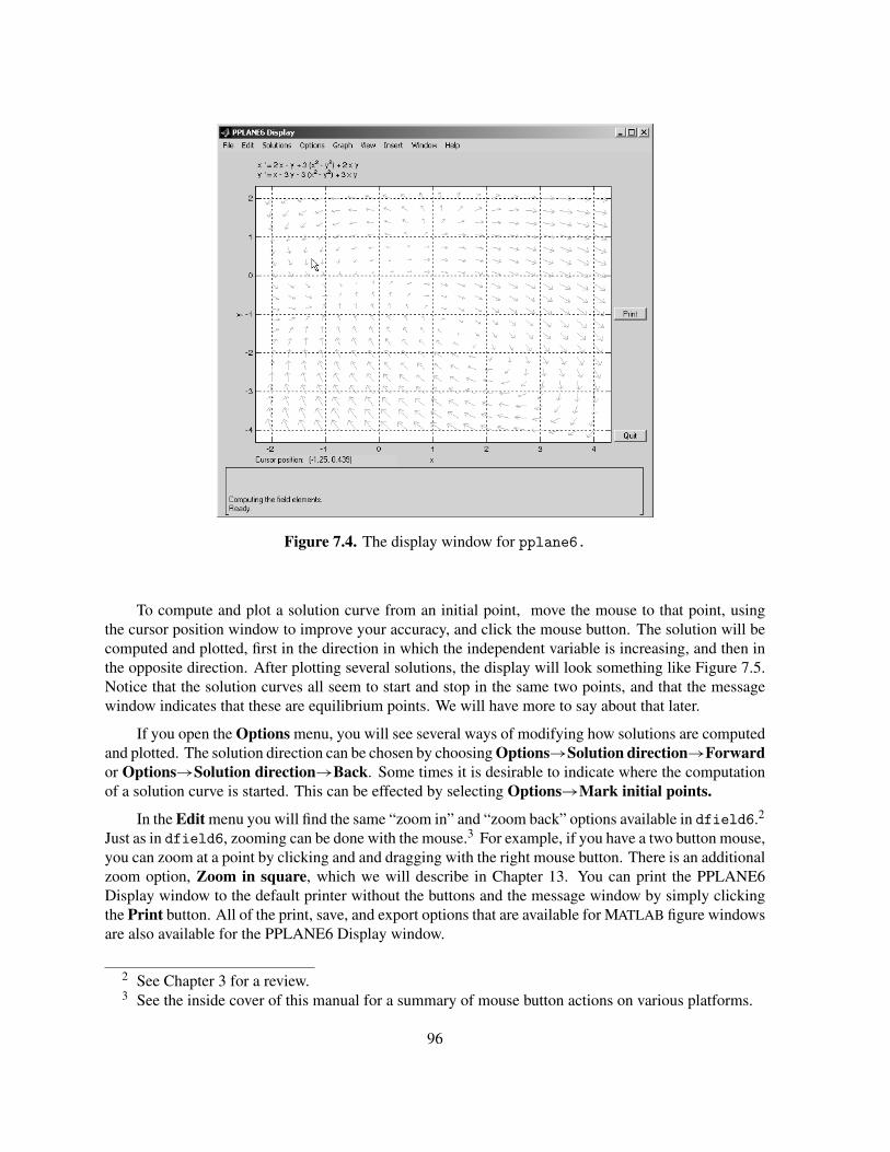
Figure 7.4. The display window for pplane6.

To compute and plot a solution curve from an initial point, move the mouse to that point, usingthe cursor position window to improve your accuracy, and click the mouse button. The solution will becomputed and plotted, first in the direction in which the independent variable is increasing, and then inthe opposite direction. After plotting several solutions, the display will look something like Figure 7.5.Notice that the solution curves all seem to start and stop in the same two points, and that the messagewindow indicates that these are equilibrium points. We will have more to say about that later.

If you open the Options menu, you will see several ways of modifying how solutions are computedand plotted. The solution direction can be chosen by choosing Options→Solution direction→Forwardor Options→Solution direction→Back. Some times it is desirable to indicate where the computationof a solution curve is started. This can be effected by selecting Options→Mark initial points.

In the Edit menu you will find the same “zoom in” and “zoom back” options available in dfield6.2

Just as in dfield6, zooming can be done with the mouse.3 For example, if you have a two button mouse,you can zoom at a point by clicking and and dragging with the right mouse button. There is an additionalzoom option, Zoom in square, which we will describe in Chapter 13. You can print the PPLANE6Display window to the default printer without the buttons and the message window by simply clickingthe Print button. All of the print, save, and export options that are available for MATLAB figure windowsare also available for the PPLANE6 Display window.

2 See Chapter 3 for a review.3 See the inside cover of this manual for a summary of mouse button actions on various platforms.

96

Figure 7.5. Several solutions to the equation.

Changing the System — Using the PPLANE6 Setup Window

We will illustrate the use of pplane6 by using it to do a phase plane analysis of the motion of apendulum. The differential equation for the motion of a pendulum is

mLd2θ

dt2 = −mg sin(θ) − cdθ

dt, (7.8)

where θ is the angular displacement of the pendulum from the vertical, L is the length of the pendulumarm, g is the acceleration due to gravity, and c is the damping constant. If we choose a convenientmeasure of time by setting s = √

g/L t , the equation becomes4

d2θ

ds2 = − sin(θ) − adθ

ds, (7.9)

wherea = c

m√

gL

is again called the damping constant. Notice that this scaling of the variables reduces the number ofparameters from four to one, and clearly indicates the importance of the lumped parameter a.

4 Hint: dθdt

= dθds

dsdt

=√

gL

dθds

; thus, d2θdt2 = g

Ld2θds2 (why?).

97

We want to write this as a first order system, so we introduce the variables

x = θ and y = dθ

ds. (7.10)

Then we have by (7.9) and (7.10)

dx

ds=dθ

ds= y,

dy

ds=d2θ

ds2 = − sin(θ) − adθ

ds= − sin(x) − ay,

(7.11)

or, more simply,x′ = y,

y′ = − sin(x) − ay,(7.12)

where the prime indicates differentiation with respect to s. This is a planar autonomous system which wecan analyze using pplane6. Enter the equations into the appropriate boxes the PPLANE6 Setup windowThis is exactly the same as it is in dfield6, except that there are two equations. See Figure 7.6.

Figure 7.6. The PPLANE6 Setup window for the pendulum equation.

Since the damping constant a is not yet a number, we will assign it a value in one of the parameterboxes. For the time being, let’s use the value a = 0. This value can be changed later to a positive numberto see the phase plane for a damped pendulum. Next we have to describe the display rectangle. Sincex = θ represents an angle, and we will want to plot a couple of full periods, we enter −10 ≤ x ≤ 10.For the dimensions in y we have to experiment. For now, −4 ≤ y ≤ 4 will do. Entering this data is justlike it is in dfield6.

Finally, we decide which kind of direction field we want and how many field points we wantdisplayed. These are available as menu options in dfield6. The choices are more important in pplane6,so they can be made directly in the PPLANE6 Setup window. Let’s keep the default values. The completedPPLANE6 Setup window for the pendulum equation is shown in Figure 7.6. Click the Proceed buttonto transfer information from the PPLANE6 Setup window to the PPLANE6 Display window and startthe computation of the direction field.

98

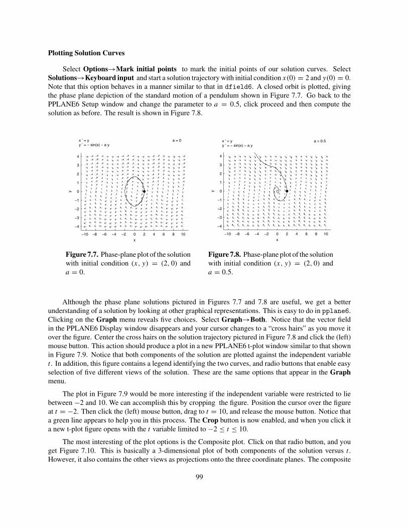
Plotting Solution Curves

Select Options→Mark initial points to mark the initial points of our solution curves. SelectSolutions→Keyboard input and start a solution trajectory with initial condition x(0) = 2 and y(0) = 0.Note that this option behaves in a manner similar to that in dfield6. A closed orbit is plotted, givingthe phase plane depiction of the standard motion of a pendulum shown in Figure 7.7. Go back to thePPLANE6 Setup window and change the parameter to a = 0.5, click proceed and then compute thesolution as before. The result is shown in Figure 7.8.

−10 −8 −6 −4 −2 0 2 4 6 8 10

−4

−3

−2

−1

0

1

2

3

4

x

y

x ’ = y y ’ = − sin(x) − a y

a = 0

−10 −8 −6 −4 −2 0 2 4 6 8 10

−4

−3

−2

−1

0

1

2

3

4

x

y

x ’ = y y ’ = − sin(x) − a y

a = 0.5

Figure 7.7. Phase-plane plot of the solutionwith initial condition (x, y) = (2, 0) anda = 0.

Figure 7.8. Phase-plane plot of the solutionwith initial condition (x, y) = (2, 0) anda = 0.5.

Although the phase plane solutions pictured in Figures 7.7 and 7.8 are useful, we get a betterunderstanding of a solution by looking at other graphical representations. This is easy to do in pplane6.Clicking on the Graph menu reveals five choices. Select Graph→Both. Notice that the vector fieldin the PPLANE6 Display window disappears and your cursor changes to a “cross hairs” as you move itover the figure. Center the cross hairs on the solution trajectory pictured in Figure 7.8 and click the (left)mouse button. This action should produce a plot in a new PPLANE6 t-plot window similar to that shownin Figure 7.9. Notice that both components of the solution are plotted against the independent variablet . In addition, this figure contains a legend identifying the two curves, and radio buttons that enable easyselection of five different views of the solution. These are the same options that appear in the Graphmenu.

The plot in Figure 7.9 would be more interesting if the independent variable were restricted to liebetween −2 and 10. We can accomplish this by cropping the figure. Position the cursor over the figureat t = −2. Then click the (left) mouse button, drag to t = 10, and release the mouse button. Notice thata green line appears to help you in this process. The Crop button is now enabled, and when you click ita new t-plot figure opens with the t variable limited to −2 ≤ t ≤ 10.

The most interesting of the plot options is the Composite plot. Click on that radio button, and youget Figure 7.10. This is basically a 3-dimensional plot of both components of the solution versus t .However, it also contains the other views as projections onto the three coordinate planes. The composite

99

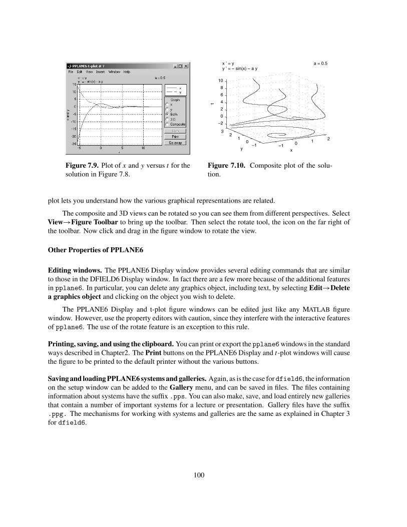
x ’ = y y ’ = − sin(x) − a y

a = 0.5

−1 0 1 2−1

01

23

−2

0

2

4

6

8

10

xy

t

Figure 7.9. Plot of x and y versus t for thesolution in Figure 7.8.

Figure 7.10. Composite plot of the solu-tion.

plot lets you understand how the various graphical representations are related.

The composite and 3D views can be rotated so you can see them from different perspectives. SelectView→Figure Toolbar to bring up the toolbar. Then select the rotate tool, the icon on the far right ofthe toolbar. Now click and drag in the figure window to rotate the view.

Other Properties of PPLANE6

Editing windows. The PPLANE6 Display window provides several editing commands that are similarto those in the DFIELD6 Display window. In fact there are a few more because of the additional featuresin pplane6. In particular, you can delete any graphics object, including text, by selecting Edit→Deletea graphics object and clicking on the object you wish to delete.

The PPLANE6 Display and t-plot figure windows can be edited just like any MATLAB figurewindow. However, use the property editors with caution, since they interfere with the interactive featuresof pplane6. The use of the rotate feature is an exception to this rule.

Printing, saving, and using the clipboard. You can print or export the pplane6windows in the standardways described in Chapter2. The Print buttons on the PPLANE6 Display and t-plot windows will causethe figure to be printed to the default printer without the various buttons.

Saving and loading PPLANE6 systems and galleries. Again, as is the case fordfield6, the informationon the setup window can be added to the Gallery menu, and can be saved in files. The files containinginformation about systems have the suffix .pps. You can also make, save, and load entirely new galleriesthat contain a number of important systems for a lecture or presentation. Gallery files have the suffix.ppg. The mechanisms for working with systems and galleries are the same as explained in Chapter 3for dfield6.

100

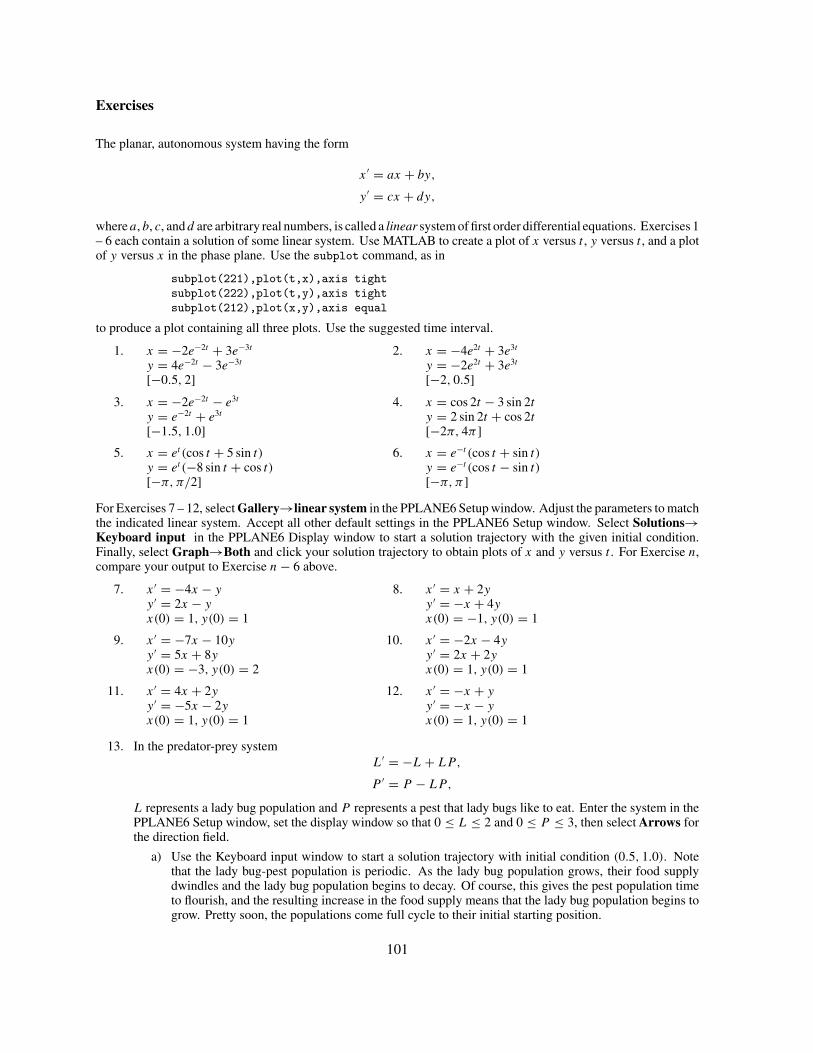
Exercises

The planar, autonomous system having the form

x ′ = ax + by,

y ′ = cx + dy,

where a, b, c, and d are arbitrary real numbers, is called a linear system of first order differential equations. Exercises 1– 6 each contain a solution of some linear system. Use MATLAB to create a plot of x versus t , y versus t , and a plotof y versus x in the phase plane. Use the subplot command, as in

subplot(221),plot(t,x),axis tight

subplot(222),plot(t,y),axis tight

subplot(212),plot(x,y),axis equal

to produce a plot containing all three plots. Use the suggested time interval.

1. x = −2e−2t + 3e−3t

y = 4e−2t − 3e−3t

[−0.5, 2]

2. x = −4e2t + 3e3t

y = −2e2t + 3e3t

[−2, 0.5]

3. x = −2e−2t − e3t

y = e−2t + e3t

[−1.5, 1.0]

4. x = cos 2t − 3 sin 2ty = 2 sin 2t + cos 2t[−2π, 4π ]

5. x = et (cos t + 5 sin t)y = et (−8 sin t + cos t)[−π, π/2]

6. x = e−t (cos t + sin t)y = e−t (cos t − sin t)[−π, π ]

For Exercises 7 – 12, select Gallery→linear system in the PPLANE6 Setup window. Adjust the parameters to matchthe indicated linear system. Accept all other default settings in the PPLANE6 Setup window. Select Solutions→Keyboard input in the PPLANE6 Display window to start a solution trajectory with the given initial condition.Finally, select Graph→Both and click your solution trajectory to obtain plots of x and y versus t . For Exercise n,compare your output to Exercise n − 6 above.

7. x ′ = −4x − yy ′ = 2x − yx(0) = 1, y(0) = 1

8. x ′ = x + 2yy ′ = −x + 4yx(0) = −1, y(0) = 1

9. x ′ = −7x − 10yy ′ = 5x + 8yx(0) = −3, y(0) = 2

10. x ′ = −2x − 4yy ′ = 2x + 2yx(0) = 1, y(0) = 1

11. x ′ = 4x + 2yy ′ = −5x − 2yx(0) = 1, y(0) = 1

12. x ′ = −x + yy ′ = −x − yx(0) = 1, y(0) = 1

13. In the predator-prey systemL′ = −L + LP,

P ′ = P − LP,

L represents a lady bug population and P represents a pest that lady bugs like to eat. Enter the system in thePPLANE6 Setup window, set the display window so that 0 ≤ L ≤ 2 and 0 ≤ P ≤ 3, then select Arrows forthe direction field.

a) Use the Keyboard input window to start a solution trajectory with initial condition (0.5, 1.0). Notethat the lady bug-pest population is periodic. As the lady bug population grows, their food supplydwindles and the lady bug population begins to decay. Of course, this gives the pest population timeto flourish, and the resulting increase in the food supply means that the lady bug population begins togrow. Pretty soon, the populations come full cycle to their initial starting position.

101

b) Suppose that the pest population is harmful to a farmer’s crop and he decides to use a poison spray toreduce the pest population. Of course, this will also kill the lady bugs. Question: Is this a wise idea?Adjust the system as follows:

L′ = −L + LP − HL,

P ′ = P − LP − HP.

Note that this model assumes that the growth rate of each population is reduced by a fixed percentageof the population. Enter this system in the PPLANE6 Setup window, but keep the original displaywindow settings. Create and set a parameter H = 0.2. Start a solution trajectory with initial condition(0.5, 1.0).

c) Repeat part b) with H = 0.4, 0.6, and 0.8. Is this an effective way to control the pests? Why?Describe what happens to each population for each value of the parameter H .

14. Enter the systemx ′ = − cos y + 2y cos y2 cos 2x

y ′ = − sin x + 2 sin y2 sin 2x

in the PPLANE6 Setup window. Set the display window to −10 ≤ x ≤ 10 and −2 ≤ y ≤ 4 and select Nonefor the vector field.

a) Select File→Save the current system and save the system with the name teddybears.pps.

b) Select Gallery→linear system to load the linear system template. Select File→Load a system andload the system teddybears.pps.

c) Select Solutions→Keyboard input and start a solution trajectory with initial condition (π/2, 0) tocreate the “legs” of the Teddy bears, and a trajectory with initial condition (−7.2, 3.5) to create the“heads” of the Teddy bears.

d) Experiment further with this “wild and wooly” example. Click the mouse in the phase plane to startother solution trajectories. Can you find the “eyes” of the Teddy bears?

When you portray sufficient solution trajectories in the phase plane so as to determine all of the important behavior ofa planar, autonomous system, you have created what is called a “phase portrait.” In Exercises 15 – 22, use pplane6

to create a phase portrait for the indicated system on the prescribed display window. Take special notice of wheresolution curves end, as reported in the message window.

15. x ′ = yy ′ = (1 − y2)y − x−3 ≤ x ≤ 3, −3 ≤ y ≤ 3

16. x ′ = y + (y2 − x2 + 0.5x4)(1 − x2)y ′ = x(1 − x2) − y(y2 − x2 + 0.5x4)−3 ≤ x ≤ 3, −2 ≤ y ≤ 2

17. x ′ = x(2y3 − x3)y ′ = −y(2x3 − y3)−3 ≤ x ≤ 3, −3 ≤ y ≤ 3

18. x ′ = y + x2 + xyy ′ = −x + xy + y2

−2 ≤ x ≤ 2, −2 ≤ y ≤ 2

19. x ′ = −y − x(x2 − y2)y ′ = −x − y(x2 − y2))−3 ≤ x ≤ 3, −3 ≤ y ≤ 3

20. x ′ = y − x(x2 + y2 − 1)y ′ = −x − y(x2 + y2 − 1)−2 ≤ x ≤ 2, −2 ≤ y ≤ 2

21. x ′ = x2 − y2

y ′ = 2xy−1 ≤ x ≤ 1, − ≤ y ≤ 1

22. x ′ = x3 − 3xy2

y ′ = 3xy2 − y3

−1 ≤ x ≤ 1, −1 ≤ y ≤ 1

The equation my ′′ + dy ′ + ky = 0 represents a damped, spring-mass system. In Exercises 23 – 26, values of theparameters m, d, and k have been chosen to create a specific example of a damped, spring-mass system. We arelooking for the solution y with the given initial position and velocity. Let

x1 = y, and x2 = y ′,

and use this change of variables to write each spring-mass system as a planar, autonomous system. Use pplane6 toobtain a printout of the graph of y versus t .

102

23. y ′′ + 2y ′ + 2y = 0y(0) = 0, y ′(0) = −1

24. y ′′ + 4y ′ + 4y = 0y(0) = −2, y ′(0) = 2

25. y ′′ + 3y ′ + 2y = 0y(0) = 3, y ′(0) = 2

26. y ′′ + 4y = 0y(0) = −4, y ′(0) = −2

27. Tanks A and B contain mixtures of water and a pollutant. Tank A has a 100 gallon capacity and is full. TankB is also full and has a 200 gallon capacity. Initially, tank A contains 40 pounds of pollutant and tank Bcontains pure water (no pollutant). At t = 0, pure water begins pouring into tank A at a rate of 10 gallons perminute. The mixture flows from tank A into tank B at a rate of 10 gallons per minute, and drains out of tankB at 10 gallons per minute. If xA and xB represent the number of pounds of pollutant in tank A and tank B,respectively, show that

x ′A = − 1

10xA,

x ′B = 1

10xA − 1

20xB,

where xA(0) = 40 and xB(0) = 0.

a) Use pplane6 and its zoom tools to estimate the maximum amount of pollutant in tank B and the timethat it occurs.

b) Use pplane6 to estimate the time that it takes the pollutant in tank B to reach a level of 10 pounds.Note: This event occurs at two separate times, once as the pollutant level is rising in tank B, and asecond time when the pollutant level is decreasing.

28. Fasten a length of string to a hook. Securely fasten a mass to the the other end of the string. Let θ represent thedisplacement of the mass from the vertical. Assume that θ is measured in radians, with positive displacementsin the counterclockwise direction. Let ω represent the angular velocity of the mass, with positive angularvelocity in the counterclockwise direction. Displace the mass 30◦ counter-clockwise (positive π/6 radians)from the vertical and release the mass from rest. Let the pendulum decay to a stable equilibrium point atθ = 0, ω = 0.

Important Note. You will not benefit as much as you should from this exercise if you don’t first completeparts a) and b) before attempting part c).

a) Without using any technology, sketch graphs of θ versus t and ω versus t approximating the motionof the pendulum.

b) Without using any technology, sketch graphs of ω versus θ . Place ω on the vertical axis, θ on thehorizontal axis. Note: This is a lot harder than it looks. We suggest that you work with a partner or agroup and compare solutions before moving on to part c).

c) Select Gallery→pendulum in the PPLANE6 Setup window. Adjust the damping parameter to D=0.1,and set the display window so that −1 ≤ θ ≤ 1 and −1 ≤ ω ≤ 1. Select Options→Solutiondirection→Forward and use the Keyboard input window to start a solution trajectory with initialcondition θ(0) = π/6 and ω(0) = 0. Compare this result with your hand-drawn solution in part b).Select Graph→Both and click your solution trajectory in the phase plane to produce plots of θ versust and ω versus t . Compare these with your hand-drawn solutions in part a).

29. Repeat the pendulum experiment of the previous problem. Displace the mass 30◦ counter-clockwise (positiveπ/6 radians) from the vertical, only this time do not release the mass from rest. Instead, push the mass in theclockwise (negative) direction with enough negative angular velocity so that it spins around in a circle exactlyone time before settling into a motion decaying to a stable equilibrium. The tricky part of this experiment isthe fact that the stable equilibrium point is now θ = −2π , ω = 0.

a) Without using any technology, sketch graphs of θ versus t and ω versus t approximating the motionof the pendulum.

b) Without using any technology, sketch graphs of ω versus θ . Place ω on the vertical axis, θ on thehorizontal axis. Note: This is a lot harder than it looks. We suggest that you work with a partner ora group and compare solutions before moving on to part c).

c) Select Gallery→pendulum in the PPLANE6 Setup window. Adjust the damping parameter to D=0.1,and set the display window so that −10 ≤ θ ≤ 5 and −4 ≤ ω ≤ 4. Select Options→Solution

103

direction→Forward and use the Keyboard input window to start a solution trajectory with initialcondition θ(0) = π/6 rad and ω(0) = −2.5 rad/s. Compare this result with your hand-drawn solutionin part b). Select Graph→Both and click your solution trajectory in the phase plane to produce plotsof θ versus t and ω versus t . Compare these with your hand-drawn solutions in part a).

30. Consider the predator-prey systemR′ = R − RF,

F ′ = −F + RF,

where R and F represent rabbit and fox populations, respectively. Enter the system in pplane6 and set thedisplay window so that 0 ≤ R ≤ 2 and 0 ≤ F ≤ 2. Use Keyboard input to start a solution trajectory atR = 0.5 and F = 1. Note that the trajectory is periodic. Use pplane6 to estimate the time it takes to travelthis periodic trajectory exactly once; i.e., find the period of the oscillation. Hint: Try cropping an x versus tplot.

31. Start a new session by exiting and restarting pplane6. Select File→Delete the current gallery in thePPLANE6 Setup window. Examine your textbook and select three planar, autonomous systems of interest.Enter the first system and set the parameters (if any), then adjust the display window and select the directionfield. Select Gallery→Add current system to the gallery to add your system to the gallery. Add each ofyour remaining systems to the gallery, then select File→Save a gallery to create and save your new gallery.

a) Start a new session by exiting and restarting pplane6. Delete the current gallery, then load your newlycreated gallery.

b) Check that each system in the gallery works as it should.

104

8. Solving ODEs in MATLAB

This is one of the most important chapters in this manual. Here we will describe how to useMATLAB’s built-in numerical solvers to find approximate solutions to almost any system of differentialequations. At this point readers might be thinking, “I’ve got dfield6 and pplane6 and I’m all set. Idon’t need to know anything further about numerical solvers.” Unfortunately, this would be far from thetruth. For example, how would we handle a system modeling a driven, damped oscillator such as

x′1 = x2,

x′2 = −2x1 − 3x2 + cos t.

(8.1)

System (8.1) is not autonomous! Pplane6 can only handle autonomous systems. Furthermore, howwould we handle a system such as

x′1 = x1 + 2x2,

x′2 = −x3 − x4,

x′3 = x1 + x3 + x4,

x′4 = −2x2 − x4.

(8.2)

The right-hand sides of system (8.2) do not explicitly involve the independent variable t , so the systemis autonomous. However, system (8.2) is not planar! Pplane6 can only handle autonomous systemsof two first order differential equations (planar systems).

Finally, in addition to handling systems of differential equations that are neither planar nor au-tonomous, we have to develop some sense of trust in the output of numerical solvers. How accurate arethey?

MATLAB’s ODE Suite

A new suite of ODE solvers was introduced with version 5 of MATLAB. The suite now contains theseven solvers ode23, ode45, ode113, ode15s, ode23s, ode23t, and ode23tb. We will spend most ofour time discussing the general purpose solver ode45. We will also briefly discuss ode15s, an excellentsolver for stiff systems. Although we will not discuss the other solvers, it is important to realize that thecalling syntax is the same for each solver in MATLAB’s suite. In the next chapter, we will discuss theMATLAB function odesolve, which puts a graphical user interface around the MATLAB solvers.

In addition to being very powerful, MATLAB’s numerical solvers are easy to use, as you will soondiscover. The methods described herein are used regularly by engineers and scientists, and are availablein any version of MATLAB. The student who learns the techniques described here will find them usefulin many later circumstances.

The ode45 solver uses a variable step Runge-Kutta procedure. Six derivative evaluations are usedto calculate an approximation of order five, and then another of order four. These are compared to comeup with an estimate of the error being made at the current step. It is required that this estimated error atany step should be less than a predetermined amount. This predetermined amount can be changed usingtwo tolerance parameters, and a very high degree of accuracy can be required of the solver. We willdiscuss this later in this chapter. For most of the uses in this Manual the default values of the toleranceparameters will provide sufficient accuracy, and we will first discuss the use of the solver with its defaultsettings.

105

Single First Order Differential Equations

We are looking at an initial value problem of the form x′ = f (t, x), with x(t0) = x0. The callingsyntax for using ode45 to find an approximate solution is ode45(odefcn,tspan,x0), where odefcncalls for a functional evaluation of f (t, x), tspan=[t0,tfinal] is a vector containing the initial andfinal times, and x0 is the x-value of the initial condition.

Example 1. Use ode45 to plot the solution of the initial value problem

x′ = cos t

2x − 2, x(0) = 3, (8.3)

on the interval [0, 2π ].

Note that equation (8.3) is in normal form x′ = f (t, x), where f (t, x) = cos t/(2x − 2). From thedata we have tspan = [0,2*pi] and x0 = 3. We need to encode the odefcn. Open your editor andcreate an ODE function M-file with the contents

function xprime = ch8examp1(t,x)xprime = cos(t)/(2*x - 2);

Save the file as ch8examp1.m. Notice that f (0, 2) = cos 0/(2 · 2 − 2) = 1/2 and

>> ch8examp1(0,2)ans =

0.5000

so the M-file gives the correct answer. If your output does not match ours, check your function code forerrors. If you still have difficulty, revisit Chapter 4, especially the discussion of the MATLAB path.

You can get a fast plot of the solution by executing ode45(@ch8examp1,[0,2*pi],3).1 Noticethat we did not specify any outputs. This causes ode45 to plot the solution. Usually you will want theoutput in order to analyze it and treat it in your own way. The following code should produce an imagesimilar to that shown in Figure 8.1.

>> [t,x] = ode45(@ch8examp1,[0,2*pi],3);>> plot(t,x)>> title('The solution of x''=cos(t)/(2x - 2), with x(0) = 3.')>> xlabel('t'), ylabel('x'), grid

The output of the ode45 command consists of a column vector t, containing the t-values at which thesolution was computed, and a column vector x containing the computed x-values.2

1 If you are using a version of MATLAB prior to version 6.0, the calling sequence should beode45(’ch8examp1’,[0,2*pi],3). We discussed this issue in Chapter 4. There are other differ-ences in the syntax to be used with MATLAB’s ODE solvers between version 6 and prior versions. Wewill emphasize the version 6 usage. For systems without parameters, users of older versions of MATLABneed only replace the function handles by the function names between single quotes. As further differ-ences arise, we will explain them, but if you are using an older version, you should execute help ode45to be sure of the correct syntax.

2 To see the output from the ode45 routine execute [t,x].

106

0 1 2 3 4 5 6 72.7

2.8

2.9

3

3.1

3.2

3.3

3.4The solution of x’ = cos(t)/(2x − 2), with x(0) = 3.

t

x

0 0.5 1 1.5 2 2.5 3 3.5 40

0.2

0.4

0.6

0.8

1

1.2

1.4

1.6

t

x

Solution of x’ = et cos x with x(0) = 0

Figure 8.1. The solution of the initial valueproblem in Example 1.

Figure 8.2. The solution of the initial valueproblem in Example 2.

Using inline functions. If you do not want to save your work, the easiest way to encode the neededodefcn is to create the inline function

>> f = inline('cos(t)/(2*x - 2)','t','x')f =

Inline function:f(t,x) = cos(t)/(2*x - 2)

We notice that f (0, 2) = 1/2, and

>> f(0,2)ans =

0.5000

so it seems to be working correctly. The command ode45(f,[0,2*pi],3) 3 will plot the solution ina figure window, with the computed points plotted as circles. Try it yourself. If you want to save thecomputed data, execute [t,x] = ode45(f,[0,2*pi],3);.

Function M-File Drivers and Subfunctions4

In Chapter 4 we explained how to use function M-files to ease the process of doing computationsand creating reproducible graphics. This technique is especially useful when using ODE solvers, as thenext example will illustrate.

Example 2. Use ode45 to plot the solution of the initial value problem

dx

dt= et cos x, x(0) = 0, (8.4)

3 Notice that we use just f when we are using an inline function. Function handles and single quotesare not needed.

4 Subfunctions were introduced in version 6 of MATLAB and are not available in earlier versions.

107

on the interval [0, 4]. Plot the computed points in a distinctive marker style as well as the curve connectingthem.

We will put all of the commands into a function M-file, with the odefcn as a subfunction. We willalso plot the computed points with dots to make them visible. Create the file

function ch8examp2close all[t,x] = ode45(@dfile,[0,4],0);plot(t,x,'.-')xlabel('t'), ylabel('x')title('Solution of x'' = e^t cos x with x(0) = 0')

function xprime = dfile(t,x)xprime = exp(t)*cos(x);

and save it as ch8examp2.m. Executing ch8examp2 will create Figure 8.2. Notice in Figure 8.2 thatthe computed points start out close to each other and then spread out for a while before becoming reallyclose to each other as t gets larger than 3. This illustrates the fact that ode45 is a variable step solver.

The file ch8examp2 is a function M-file which serves as a master routine or driver, with the ODEfunction defined as a subfunction. Subfunctions are available only within the function where they aredefined. Notice that ch8examp2 cannot be a script M-file, since subfunctions are allowed only in functionM-files.

There are several advantages to using subfunctions inside master functions in this way. Once youhave written the master file for a particular purpose, it is easy to reproduce the result. It puts everythinginvolved with a problem in one file. This file can be given a suggestive name, as we did here, to makeit easy to interpret later. With all of the commands in one file, it is relatively easy to make changes andcorrect errors. Furthermore, once you have written one such file, additional ones might well be simplemodifications of the first. Frequently, all that is needed is to change the values of the various properties.This applies to the ODE subfunction as well. There is really no need to give this subfunction a distinctivename. Call it dfile, or just f. Since the subfunction is available only within the master function it doesnot matter if it has the same name in every such file. Finally, notice that it is not really more work toproduce the file than to to execute the original commands.

Systems of First Order Equations

Actually, systems are no harder to handle using ode45 than are single equations. Consider thefollowing system of n first order differential equations:

x′1 = f1(t, x1, x2, . . . , xn),

x′2 = f2(t, x1, x2, . . . , xn),

...

x′n = fn(t, x1, x2, . . . , xn).

(8.5)

108

System (8.5) can be written in the vector form

⎡

⎢

⎢

⎣

x1x2...

xn

⎤

⎥

⎥

⎦

′

=

⎡

⎢

⎢

⎣

x′1

x′2...

x′n

⎤

⎥

⎥

⎦

=

⎡

⎢

⎢

⎣

f1(t, [x1, x2, . . . , xn]T )

f2(t, [x1, x2, . . . , xn]T )...

fn(t, [x1, x2, . . . , xn]T )

⎤

⎥

⎥

⎦

(8.6)

If we define the vector x = [x1, x2, . . . , xn]T , system (8.6) becomes

x′ =

⎡

⎢

⎢

⎣

f1(t, x)

f2(t, x)...

fn(t, x)

⎤

⎥

⎥

⎦

. (8.7)

Finally, if we define F(t, x) = [f1(t, x), f2(t, x), . . . , fn(t, x)]T , then system (8.7) can be written as

x′ = F(t, x), (8.8)

which, most importantly, has a form identical to the single first order differential equation, x′ = f (t, x),used in Example 1. Consequently, if function xprime=F(t,x) is the first line of a function ODEfile, it is extremely important that you understand that x is a vector5 with entries x(1), x(2),..., x(n).Confused? Perhaps a few examples will clear the waters.

Example 3. Use ode45 to solve the initial value problem

x′1 = x2 − x2

1 ,

x′2 = −x1 − 2x1x2,

(8.9)

on the interval [0, 10], with initial conditions x1(0) = 0 and x2(0) = 1.

We can write system (8.9) as the vector equation[

x1x2

]′=[

x2 − x21−x1 − 2x1x2

]

. (8.10)

If we set F(t, [x1, x2]T ) = [

x2 − x21 , −x1 − 2x1x2

]Tand x = [x1, x2]T , then system (8.10) takes the

form x′ = F(t, x). The key thing to realize is the fact that x = [x1, x2]T is a vector with two components,x1 and x2. Similarly, x′ = [x1

′, x2′]T is also a vector with two components, x1

′ and x2′.

Open your editor and create the following ODE file6.

function xprime = F(t,x)xprime = zeros(2,1); %The output must be a column vectorxprime(1) = x(2) - x(1)^2;xprime(2) = -x(1) - 2*x(1)*x(2);

5 In MATLAB, if x=[2;4;6;8], then x(1)=2, x(2)=4, x(3)=6, and x(4)=8.6 Even though this system is autonomous, the ODE suite does not permit you to write the first line of

the ODE file without the t variable as in function xprime=F(x). If you did, you would receive lotsof error messages.

109

Save the file as F.m. The line xprime = zeros(2,1) initializes xprime, creating a column vector withtwo rows and 1 column. Each of its entries is a zero. Note that the next two lines of the ODE file duplicateexactly what you see in system (8.9).

Even though we write x = [x1, x2]T in the narrative, it is extremely important that you understandthat x is a column vector; that is,

x =[

x1x2

]

.

Therefore, the variable x in the ODE file is also a column vector.

As always, it is an excellent idea to test that your function ODE file is working properly beforecontinuing. Because F(t, [x1, x2]T ) = [x2 − x2

1 , −x1 − 2x1x2]T , we have that F(2, [3, 4]T ) = [4 −32, −3 − 2(3)(4)]T = [−5, −27]T . Test this result at the MATLAB prompt.

>> F(2,[3;4])ans =

-5-27

Notice that the function F(t,x) expects two inputs, a scalar t and a column vector x. We used t = 2and x = [3;4]. Because this system is autonomous and independent of t , the command F(5,[3;4])should also produce [-5;-27]. Try it!

Before we call ode45, we must establish the initial condition. Recall that the initial conditions forsystem (8.9) were given as x1(0) = 0 and x2(0) = 1. Consequently, our initial condition vector will be

x(0) =[

x1(0)

x2(0)

]

=[

01

]

.

Of course, this is a column vector, so we use x0 = [0;1] or x0 = [0, 1]'. Then

>> [t,x] = ode45(@F,[0,10],[0;1]);

computes the solution.7

Typing whos at the MATLAB prompt yields8

>> whosName Size Bytes Class

t 77x1 616 double arrayx 77x2 1232 double array

Note that t and x both have 77 rows. Each row in the solution array x corresponds to a time in the samerow of the column vector t. The matrix x has two columns. The first column of x contains the solution

7 If you are working with version 5 of MATLAB, execute [t,x]=ode45(’F’,[0,10],[0;1])instead.

8 You may have more variables in your workspace than the number shown here. In addition thenumber of rows in t and x may differ from system to system.

110

for x1, while the second column of x contains the solution x2. Typing [t,x] at the MATLAB prompt andviewing the resulting output will help make this connection9.

Given a column vector v and a matrix Awhich have the same number of rows, the MATLAB commandplot(v,A) will produce a plot of each column of the matrix A versus the vector v.10 Consequently, thecommand plot(t,x) should produce a plot of each column of the matrix x versus the vector t. Thefollowing commands were used to produce the plots of x1 versus t and x2 versus t in Figure 8.3.

>> plot(t,x)>> title('x_1'' = x_2 - x_1^2 and x_2'' = -x_1 - 2x_1x_2')>> xlabel('t'), ylabel('x_1 and x_2')>> legend('x_1','x_2'), grid

Since we are limited to black and white in this Manual, the different colors of the curves are not available,so we changed the curve for x2 to a dotted linestyle. To do this we clicked the mouse button near the x2curve and selected Edit→Current Object Properties .... We then made the change of line style in theEditor.

0 1 2 3 4 5 6 7 8 9 10−0.8

−0.6

−0.4

−0.2

0

0.2

0.4

0.6

0.8

1

x1’ = x

2 − x

1

2 and x2’ = −x

1 − 2x

1x

2

t

x 1 and

x2

x1

x2

0 1 2 3 4 5 6 7 8 9 10−0.8

−0.6

−0.4

−0.2

0

0.2

0.4

0.6

x1’ = x

2 − x

1

2 and x2’ = −x

1 − 2x

1x

2

t

x 1

Figure 8.3. plot(t,x) plots both compo-nents of the solution.

Figure 8.4. plot(t,x(:,1)) plots thefirst component of the solution.

If only the first component of the solution is wanted, enter plot(t,x(:,1)). The colon in thenotation x(:,1) indicates11 that we want all rows, and the 1 indicates that we want the first column. Theresult is shown in Figure 8.4. Similarly, if only the second component is wanted, enter plot(t,x(:,2)).This is an example of the very sophisticated indexing options available in MATLAB. It is also possible toplot the components of the solution against each other with the commands

>> plot(x(:,1),x(:,2))>> title('x_1'' = x_2-x_1^2 and x_2'' = -x_1-2x_1x_2')>> xlabel('x_1'), ylabel('x_2'), grid

9 For example, note that the time values in the vector t run from 0 through 10, as they should.10 Execute help plot to see a complete description of what the plot command is capable of.11 Some MATLAB users pronounce the notation x(:,1) as “x, all rows, first column.”

111

−0.8 −0.6 −0.4 −0.2 0 0.2 0.4 0.6−0.4

−0.2

0

0.2

0.4

0.6

0.8

1

1.2

x1’ = x

2 − x

1

2 and x2’ = −x

1 − 2x

1x

2

x1

x 2

−1−0.5

00.5

1

−0.50

0.51

1.5

0

2

4

6

8

10

x1

x1’ = x

2 − x

1

2 and x2’ = −x

1 − 2x

1x

2

x2

t

Figure 8.5. Phase plane plot of the solution. Figure 8.6. 3D plot of the solution.

The result is called a phase plane plot, and it is shown in Figure 8.5.

Another way to present the solution to the system graphically is in a three dimensional plot, whereboth components of the solution are plotted as separate variables against the independent variable t .MATLAB does this using the command plot3. For example, enter plot3(t,x(:,1),x(:,2)) to seethe plot with t along the x-axis, and the two components of the solution along the y-axis and z-axis,respectively. Alternatively, enter plot3(x(:,1),x(:,2),t) to see the solution with t along the z-axis,and the two components of the solution along the x-axis and y-axis, respectively. The result of thiscommand is shown in Figure 8.6. The three dimensional graph can be rotated by first selecting therotation icon in the toolbar, and then clicking and dragging on the figure.

Solving systems with eul, rk2, and rk4. These solvers, introduced in Chapter 5, can also be used tosolve systems. The syntax for doing so is not too different from that used with ode45. For example, tosolve the system in (8.9) with eul, we use the command

>> [t,x] = eul(@F,[0,10],[0;1],h);

where h is the chosen step size. To use a different solver it is only necessary to replace eul with the rk2or rk4. Thus, the only difference between using one of these solvers and ode45 is that it is necessary toadd the step size as an additional parameter.

Second Order Differential Equations

To solve a single second order differential equation it is necessary to replace it with the equivalentfirst order system. For the equation

y′′ = f (t, y, y′), (8.11)

we set x1 = y, and x2 = y′. Then x = [x1, x2]T is a solution to the first order system

x′1 = x2,

x′2 = f (t, x1, x2).

(8.12)

112

Conversely, if x = [x1, x2]T is a solution of the system in (8.12), we set y = x1. Then we havey′ = x′

1 = x2, and y′′ = x′2 = f (t, x1, x2) = f (t, y, y′). Hence y is a solution of the equation in (8.11).

Example 4. Plot the solution of the initial value problem

y′′ + yy′ + y = 0, y(0) = 0, y′(0) = 1, (8.13)

on the interval [0, 10].

First, solve the equation in (8.13) for y′′.y′′ = −yy′ − y (8.14)

Introduce new variables for y and y′.x1 = y and x2 = y′ (8.15)

Then we have by (8.14) and (8.15),

x1′ = y′ = x2, and x2

′ = y′′ = −yy′ − y = −x1x2 − x1,

or, more simply,x′

1 = x2,

x′2 = −x1x2 − x1.

(8.16)

If we let

F(t, [x1, x2]T ) =[

x2−x1x2 − x1

]

(8.17)

and x = [x1, x2]T , then x′ = [x1′, x2

′]T and system (8.16) takes the form x′ = F(t, x).

Let’s address this example by putting everything into one master file. This file could be

function ch8examp4[t,x] = ode45(@dfile,[0,10],[0;1]);plot(t,x(:,1))title('y'''' + yy'' + y = 0, y(0) = 0, y''(0) = 1')xlabel('t'), ylabel('y'), grid

function xprime = dfile(t,x)xprime = zeros(2,1);xprime(1) = x(2);xprime(2) = -x(1)*x(2) - x(1);

Save the file as ch8examp4.m. When we execute ch8examp4 we get Figure 8.7.

Let’s examine the file ch8examp4. First notice that the subfunction dfile is the ODE file, andimplements the function F defined in (8.17). According to (8.13), the initial condition is

x(0) =[

x1(0)

x2(0)

]

=[

y(0)

y′(0)

]

=[

01

]

.

Hence the second line inch8examp4 callsode45on the equation defined in the subfunction with the properinitial conditions. It is important to note that the original question called for a solution of y′′+yy′+y = 0.Recall from (8.15) that y = x1. Consequently, the plot command in ch8examp4 will plot y versus t ,as shown in Figure 8.7. If we replace the plot command with plot(x(:,1),x(:,2)) we will get aphase-plane plot like that in Figure 8.8.

113

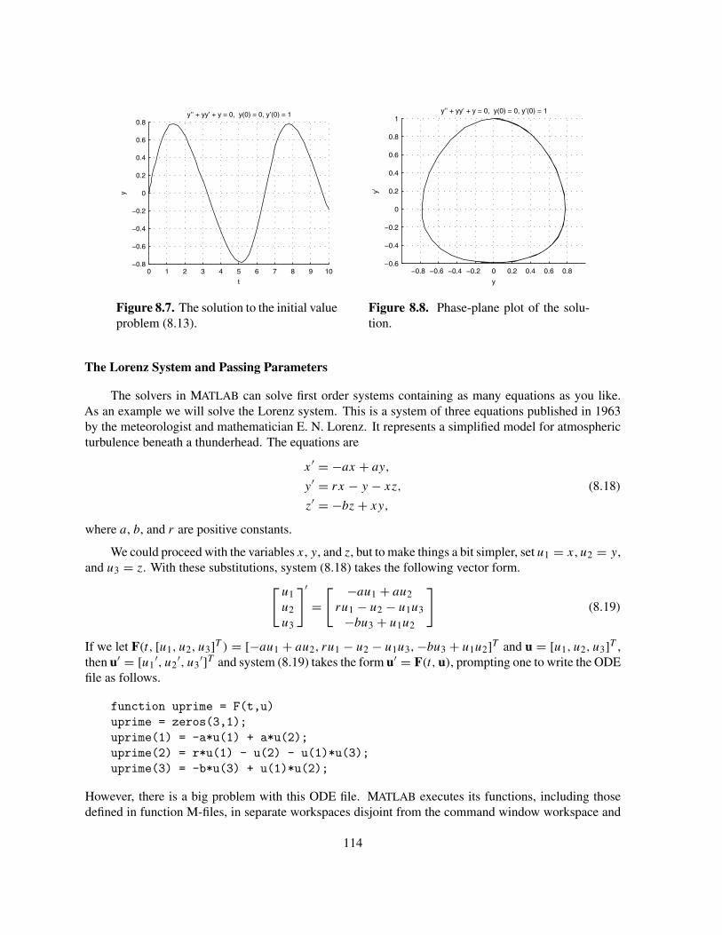
0 1 2 3 4 5 6 7 8 9 10−0.8

−0.6

−0.4

−0.2

0

0.2

0.4

0.6

0.8y’’ + yy’ + y = 0, y(0) = 0, y’(0) = 1

t

y

−0.8 −0.6 −0.4 −0.2 0 0.2 0.4 0.6 0.8−0.6

−0.4

−0.2

0

0.2

0.4

0.6

0.8

1y’’ + yy’ + y = 0, y(0) = 0, y’(0) = 1

y

y’

Figure 8.7. The solution to the initial valueproblem (8.13).

Figure 8.8. Phase-plane plot of the solu-tion.

The Lorenz System and Passing Parameters

The solvers in MATLAB can solve first order systems containing as many equations as you like.As an example we will solve the Lorenz system. This is a system of three equations published in 1963by the meteorologist and mathematician E. N. Lorenz. It represents a simplified model for atmosphericturbulence beneath a thunderhead. The equations are

x′ = −ax + ay,

y′ = rx − y − xz,

z′ = −bz + xy,

(8.18)

where a, b, and r are positive constants.

We could proceed with the variables x, y, and z, but to make things a bit simpler, set u1 = x, u2 = y,and u3 = z. With these substitutions, system (8.18) takes the following vector form.

[

u1u2u3

]′=[ −au1 + au2

ru1 − u2 − u1u3−bu3 + u1u2

]

(8.19)

If we let F(t, [u1, u2, u3]T ) = [−au1 + au2, ru1 − u2 − u1u3, −bu3 + u1u2]T and u = [u1, u2, u3]T ,then u′ = [u1

′, u2′, u3

′]T and system (8.19) takes the form u′ = F(t, u), prompting one to write the ODEfile as follows.

function uprime = F(t,u)uprime = zeros(3,1);uprime(1) = -a*u(1) + a*u(2);uprime(2) = r*u(1) - u(2) - u(1)*u(3);uprime(3) = -b*u(3) + u(1)*u(2);

However, there is a big problem with this ODE file. MATLAB executes its functions, including thosedefined in function M-files, in separate workspaces disjoint from the command window workspace and

114

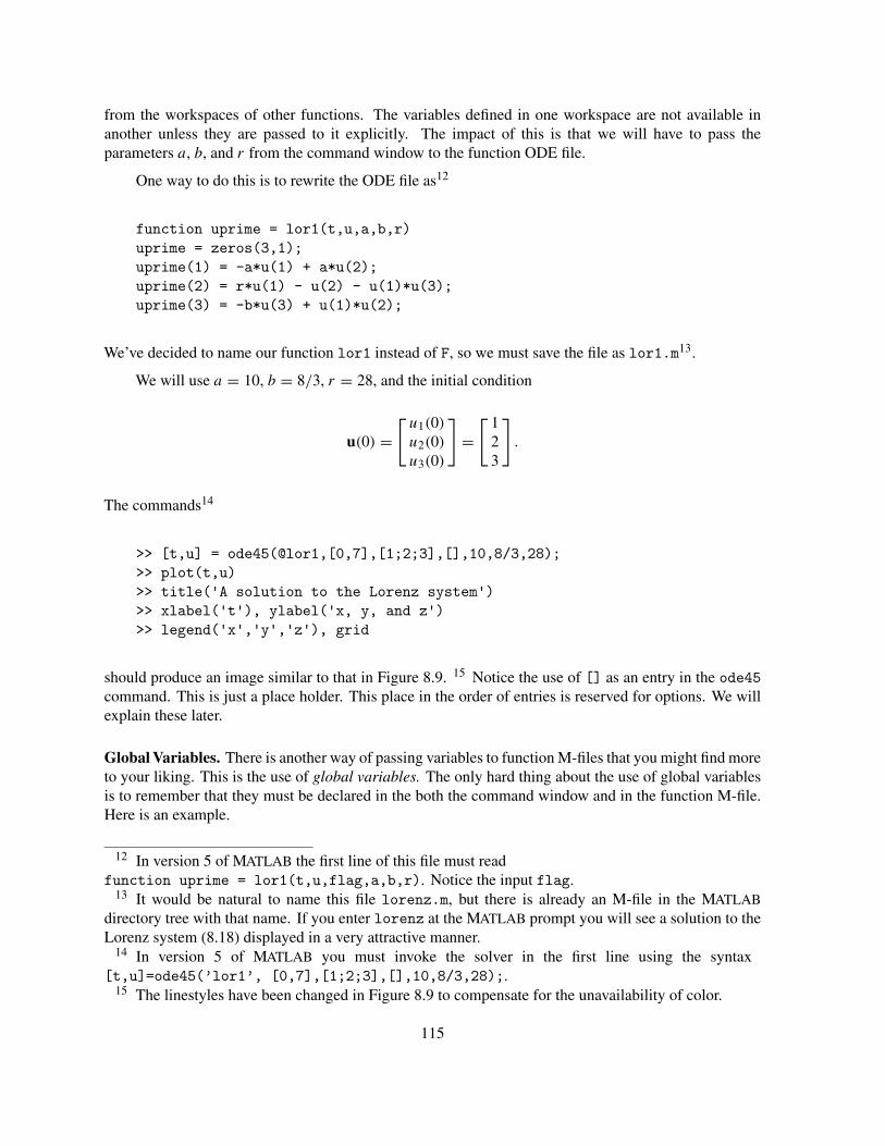
from the workspaces of other functions. The variables defined in one workspace are not available inanother unless they are passed to it explicitly. The impact of this is that we will have to pass theparameters a, b, and r from the command window to the function ODE file.

One way to do this is to rewrite the ODE file as12

function uprime = lor1(t,u,a,b,r)uprime = zeros(3,1);uprime(1) = -a*u(1) + a*u(2);uprime(2) = r*u(1) - u(2) - u(1)*u(3);uprime(3) = -b*u(3) + u(1)*u(2);

We’ve decided to name our function lor1 instead of F, so we must save the file as lor1.m13.

We will use a = 10, b = 8/3, r = 28, and the initial condition

u(0) =[

u1(0)

u2(0)

u3(0)

]

=[ 1

23

]

.

The commands14

>> [t,u] = ode45(@lor1,[0,7],[1;2;3],[],10,8/3,28);>> plot(t,u)>> title('A solution to the Lorenz system')>> xlabel('t'), ylabel('x, y, and z')>> legend('x','y','z'), grid

should produce an image similar to that in Figure 8.9. 15 Notice the use of [] as an entry in the ode45command. This is just a place holder. This place in the order of entries is reserved for options. We willexplain these later.

Global Variables. There is another way of passing variables to function M-files that you might find moreto your liking. This is the use of global variables. The only hard thing about the use of global variablesis to remember that they must be declared in the both the command window and in the function M-file.Here is an example.

12 In version 5 of MATLAB the first line of this file must readfunction uprime = lor1(t,u,flag,a,b,r). Notice the input flag.

13 It would be natural to name this file lorenz.m, but there is already an M-file in the MATLABdirectory tree with that name. If you enter lorenz at the MATLAB prompt you will see a solution to theLorenz system (8.18) displayed in a very attractive manner.

14 In version 5 of MATLAB you must invoke the solver in the first line using the syntax[t,u]=ode45(’lor1’, [0,7],[1;2;3],[],10,8/3,28);.

15 The linestyles have been changed in Figure 8.9 to compensate for the unavailability of color.

115

0 1 2 3 4 5 6 7−20

−10

0

10

20

30

40

50A solution to the Lorenz system

t

x, y

, and

z

xyz

Figure 8.9. A solution to the Lorenz system.

First change the function ODE file to

function uprime = lor2(t,u)global A B Ruprime = zeros(3,1);uprime(1) = -A*u(1) + A*u(2);uprime(2) = R*u(1) - u(2) - u(1)*u(3);uprime(3) = -B*u(3) + u(1)*u(2);

Save this second version as lor2.m. The second line declares the parameters to be global variables.Notice that we are using uppercase names for global variables. This is good practice, but is not required.

Next, we declare the global variables in the command window and initialize them

>> global A B R>> A = 10; B = 8/3; R = 28;

The global variables A, B, and R are now available in both the command window and in the workspace ofthe ODE file. You can find the numerical solution of the Lorenz system with the command16

>> [t,u] = ode45(@lor2,[0,7],[1;2;3]);

Eliminating Transient Behavior.

In many mechanical and electrical systems we experience transient behavior. This involves behaviorthat is present when the system starts, but dies out quickly in time, leaving only a fairly regular steady-state behavior. In Figure 8.9 there appears to be transient behavior until about t = 1, and then things seem

16 In version 5 of MATLAB use [t,u] = ode45(’lor2’,[0,7],[1;2;3]).

116

to settle down. To examine the situation more closely, let’s compute the solution over a longer period,say 0 ≤ t ≤ 100, and then plot the part corresponding to t > 10 in three dimensions. We would alsolike to allow for randomly chosen initial values in order to see if the steady-state behavior is somehowindependent of the initial conditions.

This is easily accomplished. The hardest part is choosing the initial conditions, and we can usethe MATLAB command rand for this. If you use help rand you will see that rand produces randomnumbers in the range [0, 1]. We want each component of our initial conditions to be randomly chosenfrom the interval [−50, 50]. It is necessary to scale the output from rand to this interval. The commandu0 = 100*(rand(3,1) - 0.5) will do the job.

Since we will want to repeat our experiment several times, we will put everything, including theODE file, into a master function M-file named loren.m. We will use global variables initialized in boththe master file and the subfunction. Including formatting commands, our file is

function loren

global A B RA = 10; B = 8/3; R = 28;u0 = 100*(rand(3,1) - 0.5);[t,u] = ode45(@lor2,[0,100],u0);N = find(t>10);v = u(N,:);plot3(v(:,1),v(:,2),v(:,3))title('The Lorenz attractor')xlabel('x'), ylabel('y'), zlabel('z')grid, shg

function uprime = lor2(t,u)global A B Ruprime = zeros(3,1);uprime(1) = -A*u(1) + A*u(2);uprime(2) = R*u(1) - u(2) - u(1)*u(3);uprime(3) = -B*u(3) + u(1)*u(2);

Further explanation is necessary. First, the command N = find(t>10); produces a list of theindices of those elements of t which satisfy t > 10. Then v = u(N,:); produces a matrix containingthe rows of u with indices in N. The result is that v consists of only those solution points corresponding tot > 10, and the resulting plot represents the long time behaviour of the solution after the transient effectsare gone.

Now, every time we execute loren we get a result very like Figure 8.10. The object in this figure isan approximation of the Lorenz attractor. The Lorenz system, with this particular choice of parameters,has the property that any solution, no matter what its initial point, is attracted to this rather complicated,butterfly-shaped, set. We will return to this in the exercises. There we will also examine the Lorenzsystem for different values of the parameters.

Click on the rotate icon in the toolbar, and click and drag the mouse in the axes in Figure 8.10 to

117

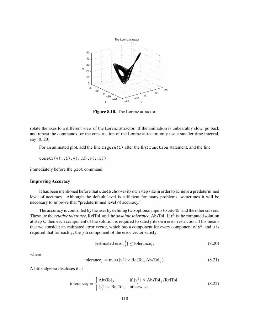
−20−10

010

20

−40−20

020

40

0

10

20

30

40

50

x

The Lorenz attractor

y

z

Figure 8.10. The Lorenz attractor.

rotate the axes to a different view of the Lorenz attractor. If the animation is unbearably slow, go backand repeat the commands for the construction of the Lorenz attractor, only use a smaller time interval,say [0, 20].

For an animated plot, add the line figure(1) after the first function statement, and the line

comet3(v(:,1),v(:,2),v(:,3))

immediately before the plot command.

Improving Accuracy

It has been mentioned before that ode45 chooses its own step size in order to achieve a predeterminedlevel of accuracy. Although the default level is sufficient for many problems, sometimes it will benecessary to improve that “predetermined level of accuracy.”

The accuracy is controlled by the user by defining two optional inputs to ode45, and the other solvers.These are the relative tolerance, RelTol, and the absolute tolerance,AbsTol. If yk is the computed solutionat step k, then each component of the solution is required to satisfy its own error restriction. This meansthat we consider an estimated error vector, which has a component for every component of yk , and it isrequired that for each j , the j th component of the error vector satisfy

|estimated error kj | ≤ tolerancej , (8.20)

wheretolerancej = max(|yk

j | × RelTol, AbsTolj ). (8.21)

A little algebra discloses that

tolerancej ={

AbsTolj , if |ykj | ≤ AbsTolj /RelTol,

|ykj | × RelTol, otherwise.

(8.22)

118

Thus the relative tolerance controls the tolerance unless |ykj | is relatively small, where “relatively small”

means |ykj | ≤ AbsTolj /RelTol.

Notice that the relative tolerance is a number, but the absolute tolerance is a vector quantity, witha component for each equation in the system being solved. This allows the user to set the tolerancedifferently for different components of the solution. The default values for RelTol is 10−3, and AbsTolis a vector, each component of which is 10−6. It is also possible to use a single number for the absolutetolerance, if the same tolerance will work for each component.

Choosing the Tolerances. The philosophy behind the use of the two tolerances is that the relativetolerance should bound the estimated error by a certain fraction of the size of the computed quantityykj for most values of that quantity. The absolute tolerance should come into play only for values of yk

j

which are small in comparison to the range of values that ykj assumes. This is to prevent the routine from

trying too hard if the computed quantity turns out to be very small at some steps. For example, with thedefaults of RelTol = 10−3 and AbsTol = 10−6, we have tolerancej = AbsTolj only when |yk

j | ≤ 10−3.

Let’s talk about choosing the relative tolerance first. This is the easier case since we are simplytalking about the number of significant digits we want in the answer. For example, the default relativetolerance is 10−3, or 0.1%. In an ideal world this will ensure that the first three digits of the computedanswer will be correct. If we want five significant digits we should choose 10−5, or 0.001%.

It would be nice if things were as simple as these considerations make them seem. Unfortunatelythe inequalities in (8.20), (8.21), and (8.22) at best control the errors made at an individual step. Theseerrors propagate, and errors made at an early step can propagate to something much larger. In fact, theerrors can propagate exponentially. The upshot is that over long time periods computational solutionscan develop serious inaccuracies. It is usually a good idea is to introduce a safety factor into your choiceof tolerances. For example if you really want three significant digits, it might be good to choose therelative tolerance smaller than 10−3, say 10−5. Even then it is imperative that you check your answerwith what you expect and reduce the tolerance even further if it seems to be called for. (See Example 5.)

To choose the absolute tolerance vector, remember that the philosophy is that the tolerance shouldbe equal to the absolute tolerance only when the computed value yk

j is small relative to the range of

values of that component. Suppose that we expect that |ykj | ≤ Mj at all computed points. Then we might

demand that AbsTol dominate the tolerance only when |ykj | ≤ 10−3 × Mj . From (8.22) we see that we

want AbsTolj /RelTol = 10−3 × Mj , so we set

AbsTolj = 10−3 × Mj × RelTol. (8.23)

Admittedly, it is usually impossible to know Mj before the solution is computed. However, one gainsinformation about this as one studies the solution. Of course the factor of 10−3 can be replaced by asmaller or larger number if the situation at hand merits it.

Let’s use these considerations to decide what tolerances to use for the Lorenz equations. Since weare only going to plot the solution, two place accuracy along the entire solution should be sufficient.Thus, the default relative tolerance of 10−3 would seem to be sufficient, but if we use a safety factor of10−2 we get a relative tolerance of 10−5. If we were to compute over longer periods of time, we mightwant to choose a smaller value, but without examining the computed results a relative tolerance smallerthan 10−5 does not seem justified.

119

To choose the absolute tolerance vector, we notice from Figures 8.9 and 8.10 that the normal rangesof the components are |x| ≤ 20, |y| ≤ 30, and |z| ≤ 40. Hence according to (8.23), we should choose

AbsTol1 ≤ 10−3 × 20 × 10−3 = 2 × 10−5,

AbsTol2 ≤ 10−3 × 30 × 10−3 = 3 × 10−5,

AbsTol3 ≤ 10−3 × 40 × 10−3 = 4 × 10−5.

We see that the default absolute tolerance of 10−6 for each seems to be adequate.

In our approach to choosing tolerances everything depends on choosing the relative tolerance. Fromour earlier discussion this seems simple enough. However, there are situations in which more accuracymay be required than appears on the surface. Suppose, for example, that it is the difference of twocomponents of the solution which is really important. To be more specific, suppose we compute asolution y, and what we are really interested in is y1 − y2, the difference of the first two componentsof y. Suppose in addition that y1 and y2 are very close to each other. Suppose in fact that we knowthey will always agree in the first 6 digits. If we set the relative tolerance to 10−7, then in an idealworld we will get 7 significant digits for y1 and y2. For example we might get y1 = 1234569 ∗ ∗ ∗ ∗ ∗and y2 = 1234563 ∗ ∗ ∗ ∗ ∗ , where the asterisks indicate digits that are not known accurately. Theny1 − y2 = 6 ∗ ∗ ∗ ∗ ∗ , so we only know 1 significant digit in the quantity we are really interested in.Consequently to get more significant digits in y1 − y2 we have to choose a smaller relative tolerance. Toget 3 significant digits we need 10−9, or with a suitable safety factor, 10−11.

Using the Tolerances in the Solvers. Having chosen our tolerances, how do we use them in ode45and the other MATLAB solvers? These solvers have many options, many more than we will describe inthis book. All of the options are input into the solver using an options vector. Suppose, for example,that we wanted to solve the Lorenz system with relative tolerance 10−5 and absolute tolerance vector[10−8, 10−7, 10−7]. We build the options vector with the command odeset, and then enter it as aparameter to ode45. If we use the first version of the Lorenz ODE file, lor1.m, then the neededcommands are

>> options = odeset('RelTol',1e-5,'AbsTol',[1e-8 1e-7 1e-7]);>> [t,u] = ode45(@lor1,[0,100],[1;2;3],options,10,8/3,28);

If the run takes inordinately long, try a shorter time span, say [0,20] instead of [0,100]. Noticethat the syntax used with ode45 is exactly the same as was used earlier for the Lorenz system, exceptthat we have inserted the parameter options between the initial conditions and the parameters sent tothe routine.

If you wish to use global variables, then use the second version of the Lorenz ODE file, lor2, with

>> options = odeset('RelTol',1e-5,'AbsTol',[1e-8 1e-7 1e-7]);>> [t,u] = ode45(@lor2,[0,100],[1;2;3],options);

Again, this assumes that you have declared the global variables and initialized them.

An experimental approach to choosing the relative tolerance. Perhaps the best way to choose therelative tolerance is illustrated by the next example.

120

Example 5. The initial value problem17

y′′ + 0.1y′ + sin y = cos t with y(0) = 0 and y′(0) = 2

models a forced damped pendulum. Use ode45 to solve the problem over the interval [0, 150].

The homogeneous problem has stable equilibria where y is an integer multiple of 2π and y′ = 0.The relatively large initial velocity, and the driving force can lead to erratic behavior. Small computingerrors can lead to incorrect solutions, as we will see. The problem is to choose an appropriate relativetolerance for ode45.

This time we will take an experimental approach to the problem. We will solve the problem witha tolerance reltol, and then solve it again with tolerance reltol/10. We will compare the twosolutions graphically, and only when they are sufficiently close will we be satisfied. The function M-fileborrelli.m will do this for us.

function borrelli(reltol)close alltspan = [0,150];velocity = 2; position = 0;color = 'r';hold onfor kk = 1:2opts = odeset('RelTol',reltol);[t,y]=ode45(@dfile,tspan,[position;velocity],opts);plot(t,y(:,1),'-','color',color)reltol = reltol/10;color = 'k';

endhold offxlabel('t'), ylabel('y')title('y'''' + 0.1y'' + sin(y) = cos(t), y(0)=0, y''(0)=2')set(gca,'YTick',-2*pi:2*pi:6*pi,...

'YTickLabel',{'-2pi','0','2pi','4pi','6pi'},...'YGrid','on')

function yprime=dfile(t,y)yprime=zeros(2,1);yprime(1) = y(2);yprime(2) = -sin(y(1)) - 0.1*y(2) + cos(t);

The file needs some explanation. The command close all closes all figures, and allows the routineto start with a clean slate each time it is used. Use this command with care, since it may close a figure

17 For more about this example, see Robert Borrelli, Courtney Coleman Computers, Lies, and theFishing Season, College Math Journal Volume 25, Number 5 (1994) and John Hubbard, The ForcedDamped Pendulum: Chaos, Complication, and Control The American Mathematical Monthly (October1999)

121

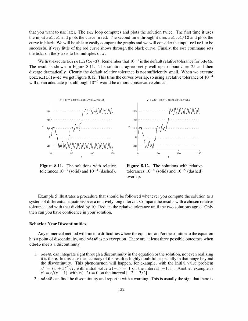
that you want to use later. The for loop computes and plots the solution twice. The first time it usesthe input reltol and plots the curve in red. The second time through it uses reltol/10 and plots thecurve in black. We will be able to easily compare the graphs and we will consider the input reltol to besuccessful if very little of the red curve shows through the black curve. Finally, the set command setsthe ticks on the y-axis to be multiples of π .

We first execute borrelli(1e-3). Remember that 10−3 is the default relative tolerance for ode45.The result is shown in Figure 8.11. The solutions agree pretty well up to about t = 25 and thendiverge dramatically. Clearly the default relative tolerance is not sufficiently small. When we executeborrelli(1e-4) we get Figure 8.12. This time the curves overlap, so using a relative tolerance of 10−4

will do an adequate job, although 10−5 would be a more conservative choice.

0 50 100 150

−2pi

0

2pi

4pi

6pi

t

y

y’’ + 0.1y’ + sin(y) = cos(t), y(0)=0, y’(0)=2

0 50 100 150

−2pi

0

2pi

4pi

6pi

t

y

y’’ + 0.1y’ + sin(y) = cos(t), y(0)=0, y’(0)=2

Figure 8.11. The solutions with relativetolerances 10−3 (solid) and 10−4 (dashed).

Figure 8.12. The solutions with relativetolerances 10−4 (solid) and 10−5 (dashed)overlap.

Example 5 illustrates a procedure that should be followed whenever you compute the solution to asystem of differential equations over a relatively long interval. Compare the results with a chosen relativetolerance and with that divided by 10. Reduce the relative tolerance until the two solutions agree. Onlythen can you have confidence in your solution.

Behavior Near Discontinuities

Any numerical method will run into difficulties where the equation and/or the solution to the equationhas a point of discontinuity, and ode45 is no exception. There are at least three possible outcomes whenode45 meets a discontinuity.

1. ode45 can integrate right through a discontinuity in the equation or the solution, not even realizingit is there. In this case the accuracy of the result is highly doubtful, especially in that range beyondthe discontinuity. This phenomenon will happen, for example, with the initial value problemx′ = (x + 3t2)/t , with initial value x(−1) = 1 on the interval [−1, 1]. Another example isx′ = t/(x + 1), with x(−2) = 0 on the interval [−2, −3/2].

2. ode45 can find the discontinuity and report it with a warning. This is usually the sign that there is

122

a discontinuity in the solution. An example of this is x′ = x2, with x(0) = 1 on the interval [0, 2].The solution is x(t) = 1/(1 − t), which has a singularity at t = 1. When asked to solve this initialvalue problem, ode45 responds with

Warning: Failure at t=9.999694e-001. Unable to meet integrationtolerances without reducing the step size below the smallestvalue allowed (3.552605e-015) at time t.

One very nice thing about ode45 is that if this happens, the output up to the point where the routinestops is made available. For example, if you execute [t,w] = ode45('gizmo',[0,3.4],[0;1; 2]);, and the computation stops because a step size is called for which is smaller than theminimum allowed, then the variables t and w will contain the results of the computation up to thatpoint.

3. ode45 can choose smaller and smaller step sizes upon the approach to a discontinuity and go oncalculating for a very long time — hours in some cases. For cases like this, it is important forthe user to know how to stop a calculation in MATLAB. On most computers the combination ofthe control key and C depressed simultaneously will do the trick. An example is x′ = t/(x + 1),with x(−10) = 2 on the interval [−10, −5]. Many stiff equations and systems will also requirean inordinate solution time using ode45.

Stiff Equations

Solutions to differential equations often have components which are varying at different rates. Ifthese rates differ by a couple of orders of magnitude, the equations are called stiff. Stiff equations willnot arise very often in this manual, but we will say a word about them in case you should have to dealwith one. We will also put some examples in the exercises.

The equation x′ = et cos x from Example 2 is stiff over relatively large time intervals, simplybecause the factor et gets very large. To see what this does to ode45, execute

>> f = inline('exp(t)*cos(x)','t','x');>> ode45(f,[0,10],0)

Since we have not required any output from ode45, it will plot the solution as it computes it. You willnotice that the speed of the plot slows up dramatically as t increases. When you are tired of waitingfor the solution to end, click on the Stop button on the lower left of the figure window. This veryslow computation is the typical response of ode45 to a stiff equation or system. The fast reaction rate,measured in this case by the factor et , requires ode45 to take extremely small steps, and therefore a longtime to complete the solution.

The MATLAB suite of ode solvers contains four routines, ode15s, ode23s, ode23t, and ode23tb,which are designed to solve stiff equations. ode15s is the first of these to try. To see what it does in thiscase, execute

>> ode15s(f,[0,10],0)

Since it is designed specifically for stiff systems, it completes its work in seconds. Notice that the callingsyntax for ode15s is identical to that of ode45. This is a feature of all of the solvers in the ODE suite.

123

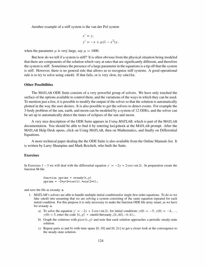
Another example of a stiff system is the van der Pol system

x′ = y,

y′ = −x + µ(1 − x2)y,

when the parameter µ is very large, say µ = 1000.

But how do we tell if a system is stiff? It is often obvious from the physical situation being modeledthat there are components of the solution which vary at rates that are significantly different, and thereforethe system is stiff. Sometimes the presence of a large parameter in the equations is a tip off that the systemis stiff. However, there is no general rule that allows us to recognize stiff systems. A good operationalrule is to try to solve using ode45. If that fails, or is very slow, try ode15s.

Other Possibilities

The MATLAB ODE Suite consists of a very powerful group of solvers. We have only touched thesurface of the options available to control them, and the variations of the ways in which they can be used.To mention just a few, it is possible to modify the output of the solver so that the solution is automaticallyplotted in the way the user desires. It is also possible to get the solvers to detect events. For example the3-body problem of the sun, earth, and moon can be modeled by a system of 12 ODEs, and the solver canbe set up to automatically detect the times of eclipses of the sun and moon.

A very nice description of the ODE Suite appears in Using MATLAB, which is part of the MATLABdocumentation. You should be able to find it by entering helpdesk at the MATLAB prompt. After theMATLAB Help Desk opens, click on Using MATLAB, then on Mathematics, and finally on DifferentialEquations.

A more technical paper dealing the the ODE Suite is also available from the Online Manuals list. Itis written by Larry Shampine and Mark Reichelt, who built the Suite.

Exercises

In Exercises 1 – 3 we will deal with the differential equation y ′ = −2y + 2 cos t sin 2t . In preparation create thefunction M-file

function yprime = steady(t,y)

yprime = -2*y+2*cos(t).*sin(2*t);

and save the file as steady.m.

1. MATLAB’s solvers are able to handle multiple initial conditionsfor single first order equations. To do so wefake ode45 into assuming that we are solving a system consisting of the same equation repeated for eachinitial condition. For this purpose it is only necessary to make the function ODE file array smart, as we havefor steady.m.

a) To solve the equation y ′ = −2y + 2 cos t sin 2t , for initial conditions y(0) = −5, y(0) = −4,. . . ,y(0) = 5, enter the code [t,y] = ode45(@steady,[0,30],-5:5);.

b) Graph the solutions with plot(t,y) and note that each solution approaches a periodic steady-statesolution.

c) Repeat parts a) and b) with time spans [0, 10] and [0, 2π ] to get a closer look at the convergence tothe steady-state solution.

124

2. Another nice feature of MATLAB’s solvers is the ability to output solutions at specified times. This isuseful when you want to compare two functions at specified time points or place the output from mul-tiple calls to ode45 in a matrix, where it is required that the rows have equal length. Enter [t,y] =

ode45(@steady,0:.25:3,1);, then enter [t,y]. This should clarify what is going on.

3. MATLAB’s solvers can automatically plot solutions as they are computed. All you need to do is leave off theoutput variables when calling the solver. Try ode45('steady',[0,30],-5:5).

In Exercises 4 – 7, plot the solutions to all of the initial value problems on one figure. Choose a solution intervalstarting at t = 0 that well illustrates any steady-state phenomena that you see. Exercise 1 might be helpful.

4. y ′ + 4y = 2 cos t + sin 4t , with y(0) = −5, −4, . . . , 5.

5. y ′ + 4y = t2, with y(0) = −9, −8, −7, −1, 1, 7, 8, 9.

6. x ′ = cos t − x3, with x(0) = −3, −2, . . . , 3.

7. x ′ + x + x3 = cos2 t, with x(0) = −3, −2, . . . , 3.

8. Separate variables and find an explicit solution of x ′ = t/(1 + x), x(0) = 1.

a) Use ode45 to find the numerical solution of the initial value problem on the interval [0, 3]. Store thesolution in the variables t and x_ode45.

b) Use the explicit solution to find exact solution values at each point in the vector t obtained in part a).Store the results in the variable x_exact. Compare the solutions graphically with plot(t, x_exact,

t, x_ode45,'r.'). Obtain a printout with a legend.

c) For a finer graphical image of the error plot x_exact - x_ode45 versus t in a new figure. Pay specialattention to the dimensions on the y-axis.

In Exercises 9 – 12, write a function ODE file for the system. Solve the initial value problem using ode45. Provideplots of x1 versus t , x2 versus t , and x2 versus x1 on the time interval provided. See Exercises 1 – 6 in Chapter 7 fora nice method to arrange these plots.

9. x1′ = x2 and x2

′ = (1 − x12)x2 − x1, with x1(0) = 0 and x2(0) = 4 on [0, 10].

10. x1′ = x2 and x2

′ = −25x1 + 2 sin 4t , with x1(0) = 0 and x2(0) = 2 on [0, 2π ].

11. x1′ = (x2 + x1/5)(1 − x2

1 ) and x2′ = −x1(1 − x2

2 ), with x1(0) = 0.8 and x2(0) = 0 on [0, 30].

12. x1′ = x2 and x2

′ = −x1 + x2(1 − 3x21 − 3x2

2 ), with x1(0) = 0.2 and x2(0) = 0.2 on [0, 20].

13. The built-in plotting routines of MATLAB’s solvers were illustrated in Exercise 3. They work equally wellwith systems. For example, create

function yprime = heart(t,y)

yprime = zeros(2,1);

yprime(1) = y(2);

yprime(2) = -16*y(1)+4*sin(2*t);

and save as heart.m.

a) Enter ode45(@heart,[0,2*pi],[0;2]) and note that MATLAB dynamically plots both y1 and y2

versus t .

b) To change the output routine, enter options = odeset('OutputFcn','odephas2'), followed byode45(@heart,[0,2*pi],[0;2],options). Note that MATLAB dynamically plots y2 versus y1 inthe phase plane.

14. Use the technique of Example 4 to change the initial value problem yy ′′ − (y ′)2 −y2 = 0, y(0) = 1, y ′(0) =−1 to a system with initial conditions. Use ode45 to create a plot of y versus t .

15. An unforced spring-mass system with no damping can be modeled by the equation y ′′ + ky = 0, where kis the spring constant. However, suppose that the spring loses elasticity with time. A possible model foran “aging” spring-mass system is y ′′ + 2e−0.12t y = 0. Suppose that the spring is stretched two units fromequilibrium and released from rest. Use the technique of Example 4 to plot a solution of y versus t on thetime interval [0, 100].

125

16. The equation x ′′ = ax ′ − b(x ′)3 − kx was devised by Lord Rayleigh to model the motion of the reed in aclarinet. With a = 5, b = 4, and k = 5, solve this equation numerically with initial conditions x(0) = A, andx ′(0) = 0 over the interval [0, 10] for the three choices A = 0.5, 1, and 2. Use MATLAB’s hold commandto prepare both time plots and phase plane plots containing the solutions to all three initial value problemssuperimposed. Describe the relationship that you see between the three solutions.

17. Consider the forced, damped oscillator y ′′+0.05y ′+36y = sin 6.3t , with initial conditions y(0) = 5, y ′(0) =0. Use the technique of Example 4 to transform the equation to system of first order ODEs, write and savethe odefile as osc.m, and solve the system with the command [t,x] = ode45(@osc,[0,100],[5;0]);.

a) The command plot3(x(:,1),x(:,2),t) provides a three dimensional plot with time on the verticalaxis.

b) The command close all, comet3(x(:,1),x(:,2),t) provides an animated view of the result inpart a).

18. Consider the forced, undamped oscillator modeled by the equation y ′′ + ω02y = 2 cos ωt . The parameter

ω0 is the natural frequency of the unforced system y ′′ + ω02y = 0. Write an ODE function M-file for this

equation with natural frequency ω0 = 2, and the driving frequency ω passed as a parameter.

a) If the driving frequency nearly matches the natural frequency, then a phenomenon called beats occurs.As an example, solve the equation using ode45 with y(0) = 0 and y ′(0) = 0 over the interval [0, 60π ]with ω = 1.9.

b) If the driving frequency matches the natural frequency, then a phenomenon called resonance occurs.As an example, solve the equation using ode45 with y(0) = 0 and y ′(0) = 0 over the interval [0, 60π ]with ω = 2.

c) Use the plot3 and comet3 commands, as described in Exercise 17, to create three dimensional plotsof the output in parts a) and b).

19. Harmonic motion. An unforced, damped oscillator is modeled by the equation

my ′′ + cy ′ + ky = 0,

where m is the mass, c is the damping constant, and k is the spring constant. Write the equation as a systemof first order ODEs and create a function ODE file that allows the passing of parameters m, c, and k. In eachof the following cases compute the solution with initial conditions y(0) = 1, and y ′(0) = 0 over the interval[0, 20]. Prepare both a plot of y versus t and a phase plane plot of y ′ versus y.

a) (No damping) m = 1, c = 0, and k = 16.

b) (Under damping) m = 1, c = 2, and k = 16.

c) (Critical damping) m = 1, c = 8, and k = 16.

d) (Over damping) m = 1, c = 10, and k = 16.

20. The system

εdx

dt= x(1 − x) − (x − q)

(q + x)f z,

dz

dt= x − z,

models a chemical reaction called an oregonator. Suppose that ε = 10−2 and q = 9 × 10−5. Put the systeminto normal form and write an ODE function M-file for the system that passes f as a parameter. The idea isto vary the parameter f and note its affect on the solution of the oregonator model. We will use the initialconditions x(0) = 0.2 and y(0) = 0.2 and the solution interval [0, 50].

a) Use ode45 to solve the system with f = 1/4. This should provide no difficulties.

b) Use ode45 to solve the system with f = 1. This should set off all kinds of warning messages.

c) Try to improve the accuracy with options = odeset('RelTol',1e-6) and using options as theoptions parameter in ode45. You should find that this slows computation to a crawl as the system isvery stiff.

126

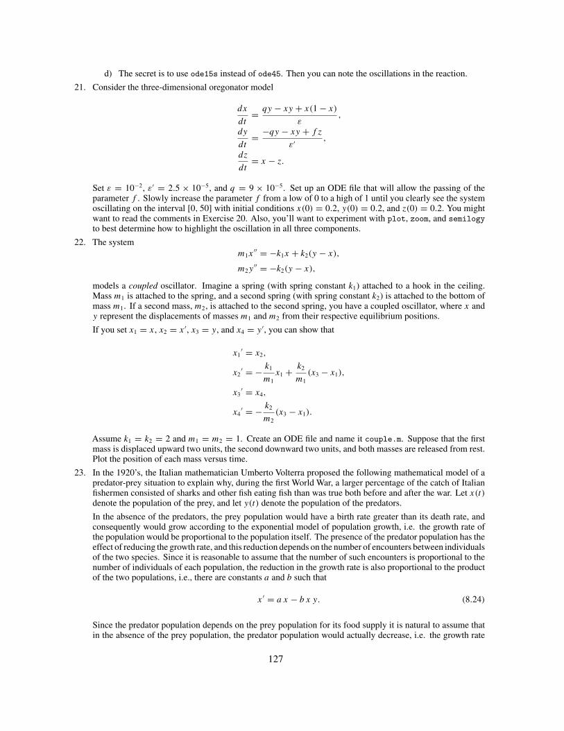
d) The secret is to use ode15s instead of ode45. Then you can note the oscillations in the reaction.

21. Consider the three-dimensional oregonator model

dx

dt= qy − xy + x(1 − x)

ε,

dy

dt= −qy − xy + f z

ε′ ,

dz

dt= x − z.

Set ε = 10−2, ε′ = 2.5 × 10−5, and q = 9 × 10−5. Set up an ODE file that will allow the passing of theparameter f . Slowly increase the parameter f from a low of 0 to a high of 1 until you clearly see the systemoscillating on the interval [0, 50] with initial conditions x(0) = 0.2, y(0) = 0.2, and z(0) = 0.2. You mightwant to read the comments in Exercise 20. Also, you’ll want to experiment with plot, zoom, and semilogy

to best determine how to highlight the oscillation in all three components.

22. The systemm1x

′′ = −k1x + k2(y − x),

m2y′′ = −k2(y − x),

models a coupled oscillator. Imagine a spring (with spring constant k1) attached to a hook in the ceiling.Mass m1 is attached to the spring, and a second spring (with spring constant k2) is attached to the bottom ofmass m1. If a second mass, m2, is attached to the second spring, you have a coupled oscillator, where x andy represent the displacements of masses m1 and m2 from their respective equilibrium positions.

If you set x1 = x, x2 = x ′, x3 = y, and x4 = y ′, you can show that

x1′ = x2,

x2′ = − k1

m1x1 + k2

m1(x3 − x1),

x3′ = x4,

x4′ = − k2

m2(x3 − x1).

Assume k1 = k2 = 2 and m1 = m2 = 1. Create an ODE file and name it couple.m. Suppose that the firstmass is displaced upward two units, the second downward two units, and both masses are released from rest.Plot the position of each mass versus time.

23. In the 1920’s, the Italian mathematician Umberto Volterra proposed the following mathematical model of apredator-prey situation to explain why, during the first World War, a larger percentage of the catch of Italianfishermen consisted of sharks and other fish eating fish than was true both before and after the war. Let x(t)denote the population of the prey, and let y(t) denote the population of the predators.

In the absence of the predators, the prey population would have a birth rate greater than its death rate, andconsequently would grow according to the exponential model of population growth, i.e. the growth rate ofthe population would be proportional to the population itself. The presence of the predator population has theeffect of reducing the growth rate, and this reduction depends on the number of encounters between individualsof the two species. Since it is reasonable to assume that the number of such encounters is proportional to thenumber of individuals of each population, the reduction in the growth rate is also proportional to the productof the two populations, i.e., there are constants a and b such that

x ′ = a x − b x y. (8.24)

Since the predator population depends on the prey population for its food supply it is natural to assume thatin the absence of the prey population, the predator population would actually decrease, i.e. the growth rate

127

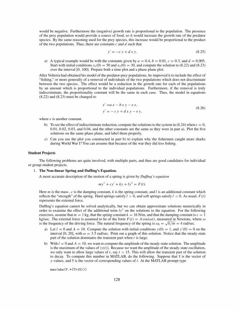
would be negative. Furthermore the (negative) growth rate is proportional to the population. The presenceof the prey population would provide a source of food, so it would increase the growth rate of the predatorspecies. By the same reasoning used for the prey species, this increase would be proportional to the productof the two populations. Thus, there are constants c and d such that

y ′ = −c y + d x y. (8.25)

a) A typical example would be with the constants given by a = 0.4, b = 0.01, c = 0.3, and d = 0.005.Start with initial conditions x1(0) = 50 and x2(0) = 30, and compute the solution to (8.22) and (8.23)over the interval [0, 100]. Prepare both a time plot and a phase plane plot.

After Volterra had obtained his model of the predator-prey populations, he improved it to include the effect of“fishing,” or more generally of a removal of individuals of the two populations which does not discriminatebetween the two species. The effect would be a reduction in the growth rate for each of the populationsby an amount which is proportional to the individual populations. Furthermore, if the removal is trulyindiscriminate, the proportionality constant will be the same in each case. Thus, the model in equations(8.22) and (8.23) must be changed to

x ′ =a x − b x y − e x,

y ′ = − c y + d x y − e y,(8.26)

where e is another constant.

b) To see the effect of indiscriminate reduction, compute the solutions to the system in (8.24) when e = 0,0.01, 0.02, 0.03, and 0.04, and the other constants are the same as they were in part a). Plot the fivesolutions on the same phase plane, and label them properly.

c) Can you use the plot you constructed in part b) to explain why the fishermen caught more sharksduring World War I? You can assume that because of the war they did less fishing.

Student Projects

The following problems are quite involved, with multiple parts, and thus are good candidates for individualor group student projects.

1. The Non-linear Spring and Duffing’s Equation.

A more accurate description of the motion of a spring is given by Duffing’s equation

my ′′ + cy ′ + ky + ly3 = F(t).

Here m is the mass , c is the damping constant, k is the spring constant, and l is an additional constant whichreflects the “strength” of the spring. Hard springs satisfy l > 0, and soft springs satisfy l < 0. As usual, F(t)represents the external force.

Duffing’s equation cannot be solved analytically, but we can obtain approximate solutions numerically inorder to examine the effect of the additional term ly3 on the solutions to the equation. For the followingexercises, assume that m = 1 kg, that the spring constant k = 16 N/m, and that the damping constant is c = 1kg/sec. The external force is assumed to be of the form F(t) = A cos(ωt), measured in Newtons, where ωis the frequency of the driving force. The natural frequency of the spring is ω0 = √

k/m = 4 rad/sec.

a) Let l = 0 and A = 10. Compute the solution with initial conditions y(0) = 1, and y ′(0) = 0 on theinterval [0, 20], with ω = 3.5 rad/sec. Print out a graph of this solution. Notice that the steady-statepart of the solution dominates the transient part when t is large.

b) With l = 0 and A = 10, we want to compute the amplitude of the steady-state solution. The amplitudeis the maximum of the values of |y(t)|. Because we want the amplitude of the steady-state oscillation,we only want to allow large values of t , say t > 15. This will allow the transient part of the solutionto decay. To compute this number in MATLAB, do the following. Suppose that Y is the vector ofy-values, and T is the vector of corresponding values of t . At the MATLAB prompt type

max(abs(Y.*(T>15)))

128

Your answer will be a good approximation to the amplitude of the steady-state solution.

Why is this true? The expression (T>15) yields a vector the same size as T, and an element of thisvector will be 1 if the corresponding element of T is larger than 15 and 0 otherwise. Thus Y.*(T>15)is a vector the same size as T or Y with all of the values corresponding to t ≤ 15 set to 0, and the othervalues of Y left unchanged. Hence, the maximum of the absolute values of this vector is just what wewant.

Set up a script M-file that will allow you to do the above process repeatedly. For example, if thederivative M-file for Duffing’s equation is called duff.m, the script M-file could be

[t,y] = ode45(@duff'0,20,[1,0]);y = y(:,1);

amplitude = max(abs(y.*(t>15)))

Now by changing the value of ω in duff.m you can quickly compute how the amplitude changeswith ω. Do this for eight evenly spaced values of ω between 3 and 5. Use plot to make a graph ofamplitude vs. frequency. For approximately what value of ω is the amplitude the largest?

c) Set l = 1 (the case of a hard spring) and A = 10 in Duffing’s equation and repeat b). Find the valueof ω, accurate to 0.2 rad/sec, for which the amplitude reaches its maximum.

d) For the hard spring in c), set A = 40. With y(0) = y ′(0) = 0, and for eight (or more) evenly spacedvalues of ω between 5 and 7 compute the magnitude of the steady-state oscillation. Plot the graph ofamplitude vs. frequency. Repeat the computation with initial conditions y(0) = 6, y ′(0) = 0, and plotthe two graphs of amplitude vs. frequency on the same figure. (The phenomenon you will observe iscalled Duffing’s hysteresis.)

e) Set l = −1 and A = 10 (the case of a soft spring) in Duffing’s equation and repeat c).

2. The Lorenz System.

The purpose of this exercise is to explore the complexities displayed by the Lorenz system as the parametersare varied. We will keep a = 10, and b = 8/3, and vary r . For each value of r , examine the behavior of thesolution with different initial conditions, and make conjectures about the limiting behavior of the solutions ast → ∞. The solutions should be plotted in a variety of ways in order to get the information. These includetime plots, such as Figure 8.9, and phase space plots, such as Figure 8.10. In the case of phase space plots,use the rotate3d command to capture a view of the system that provides the best visual information. Youmight also use other plots, such as z versus x, etc.

Examine the Lorenz system for a couple of values of r in each of the following intervals. Describe the limitingbehavior of the solutions.

a) 0 < r < 1.

b) 1 < r < 470/19. There are two distinct cases.

c) 470/19 < r < 130. The case done in the text. This is a region of chaotic behavior of the solutions.

d) 150 < r < 165. Things settle down somewhat.

e) 215 < r < 280. Things settle down even more.

3. Motion Near the Lagrange Points.

Consider two large spherical masses of mass M1 > M2. In the absence of other forces, these bodies willmove in elliptical orbits about their common center of mass (if it helps, think of these as the earth and themoon). We will consider the motion of a third body (perhaps a spacecraft), with mass which is negligible incomparison to M1 and M2, under the gravitational influence of the two larger bodies. It turns out that there arefive equilibrium points for the motion of the small body relative to the two larger bodies. Three of these werefound by Euler, and are on the line connecting the two large bodies. The other two were found by Lagrangeand are called the Lagrange points. Each of these forms an equilateral triangle in the plane of motion withthe positions of the two large bodies. We are interested in the motion of the spacecraft when it starts near aLagrange point.

129

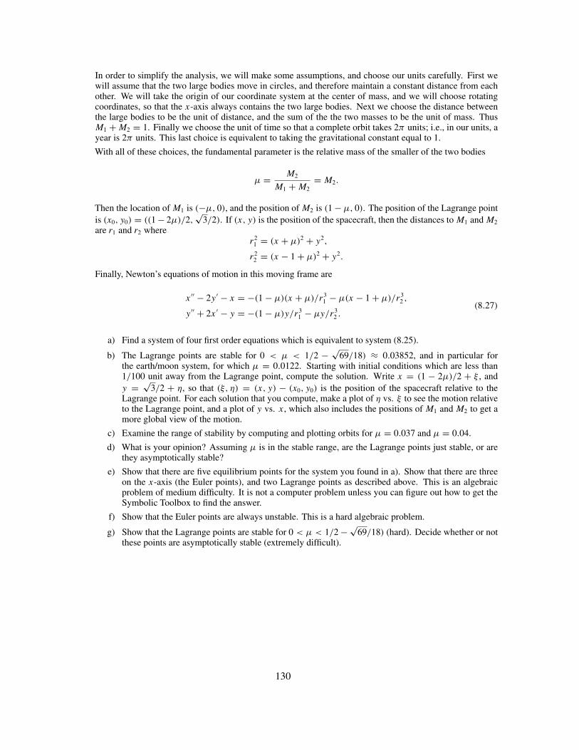
In order to simplify the analysis, we will make some assumptions, and choose our units carefully. First wewill assume that the two large bodies move in circles, and therefore maintain a constant distance from eachother. We will take the origin of our coordinate system at the center of mass, and we will choose rotatingcoordinates, so that the x-axis always contains the two large bodies. Next we choose the distance betweenthe large bodies to be the unit of distance, and the sum of the the two masses to be the unit of mass. ThusM1 + M2 = 1. Finally we choose the unit of time so that a complete orbit takes 2π units; i.e., in our units, ayear is 2π units. This last choice is equivalent to taking the gravitational constant equal to 1.

With all of these choices, the fundamental parameter is the relative mass of the smaller of the two bodies

µ = M2

M1 + M2= M2.

Then the location of M1 is (−µ, 0), and the position of M2 is (1 − µ, 0). The position of the Lagrange pointis (x0, y0) = ((1 − 2µ)/2,

√3/2). If (x, y) is the position of the spacecraft, then the distances to M1 and M2

are r1 and r2 wherer2

1 = (x + µ)2 + y2,

r22 = (x − 1 + µ)2 + y2.

Finally, Newton’s equations of motion in this moving frame are

x ′′ − 2y ′ − x = −(1 − µ)(x + µ)/r31 − µ(x − 1 + µ)/r3

2 ,

y ′′ + 2x ′ − y = −(1 − µ)y/r31 − µy/r3

2 .(8.27)

a) Find a system of four first order equations which is equivalent to system (8.25).

b) The Lagrange points are stable for 0 < µ < 1/2 − √69/18) ≈ 0.03852, and in particular for

the earth/moon system, for which µ = 0.0122. Starting with initial conditions which are less than1/100 unit away from the Lagrange point, compute the solution. Write x = (1 − 2µ)/2 + ξ , andy = √

3/2 + η, so that (ξ, η) = (x, y) − (x0, y0) is the position of the spacecraft relative to theLagrange point. For each solution that you compute, make a plot of η vs. ξ to see the motion relativeto the Lagrange point, and a plot of y vs. x, which also includes the positions of M1 and M2 to get amore global view of the motion.

c) Examine the range of stability by computing and plotting orbits for µ = 0.037 and µ = 0.04.

d) What is your opinion? Assuming µ is in the stable range, are the Lagrange points just stable, or arethey asymptotically stable?

e) Show that there are five equilibrium points for the system you found in a). Show that there are threeon the x-axis (the Euler points), and two Lagrange points as described above. This is an algebraicproblem of medium difficulty. It is not a computer problem unless you can figure out how to get theSymbolic Toolbox to find the answer.

f) Show that the Euler points are always unstable. This is a hard algebraic problem.

g) Show that the Lagrange points are stable for 0 < µ < 1/2 − √69/18) (hard). Decide whether or not

these points are asymptotically stable (extremely difficult).

130

9. Introduction to ODESOLVE

The MATLAB function odesolve1 provides a way to use MATLAB’s solvers with a graphical userinterface. It can be applied to any system of first order equations, and therefore to any system of anyorder. The dimension of the system is limited only by the size of the computer screen. Since it has agraphical interface, it is relatively easy to use, but the interface does present limitations as well.

Starting odesolve

The interface of odesolve is very similar to those found in dfield and pplane. To begin, execute

>> odesolve

at the MATLAB prompt. This opens the ODESOLVE Setup window. An example can be seen inFigure 9.2. The similarities with dfield and pplane are clear. However there are differences as well.One of the most important is the edit box for the number of equations. Change this number to 20 anddepress the Tab or Enter key. The setup window expands to allow the entry of 20 equations and thecorresponding initial conditions.

Example 1. Consider the two masses m1 and m2 connected by springs and driven by an external force, asillustrated in Figure 9.1. In the absence of the force, each of the masses has an equilibrium position. Letx and y denote the displacements of the masses from their equilibrium positions, as shown in Figure 9.1.Plot the displacements for a variety of values of the parameters and external forces.

Analysis of the forces and Newton’s second law lead us to the system of equations

m1x′′ = k2(y − x) − k1x,

m2y′′ = −k2(y − x) + f (t),

(9.1)

where k1 and k2 are the spring constants, and f (t) is the external force.

m1 m2

k1 k2

f (t)

x(t) y(t)

Figure 9.1. Coupled oscillators with a driving force.

1 Odesolve is not part of the MATLAB distribution. Consult the appendix to Chapter 3 to learn howto obtain it.

131

If we introduce the velocities u = x′ and v = y′, the system in (9.1) is equivalent to the first ordersystem

x′ = u,

u′ = (k2(y − x) − k1x)/m1,

y′ = v,

v′ = (−k2(y − x) + f (t))/m2.

(9.2)

This is the system we want to solve using odesolve. To do so, we change the number of equations to 4,and then enter the differential equations. We can speed the process by executing Gallery→two springs.The result is shown in Figure 9.2. Notice that the equations are entered almost like they appear in (9.2).

Figure 9.2. The setup window for odesolve.

Values for the initial conditions have been entered. The spring constants and the masses have beengiven values in the parameter edit boxes. The force f (t) = A cos(ωt) has been entered as an expression,while values for the amplitude A and frequency ω have been entered in parameter boxes. In odesolve,the parameters must be numbers, but expressions can be any algebraic expression involving the variablesand the parameters.

It is also true that the initial conditions can use the parameters, but that does not occur in this case.You will notice that we did not use TEX notation for the subscripted string constants and masses. TEXnotation is allowed for variable names, but not for the names of parameters and expressions.

The independent variable has been identified as t . It has been given an initial value, and a solutioninterval has been designated.

Near the bottom of the setup window, we see that ode45 is the solver that will be used. This can bechanged to any of the MATLAB solvers using the popup menu. We are also told that the output will beall variables plotted against t . This can also be changed using the popup menu. For the time being let’sleave these settings as they are.

132

To start a solution, click on the button Solve in a new window. After a few seconds, we get a plotof all four components of the solution to (9.2) plotted against t . Even with the legend, this figure is alittle busy. We are really interested in the displacements, so let’s go back to the setup window and selecttime plot from the output popup menu. Do so even though it looks like it is already selected. In thelittle window that appears, select only x and y, and then click Change. Click on Solve in a new windowagain. The result is shown in Figure 9.3.

xy

0 5 10 15 20 25 30

−2.5

−2

−1.5

−1

−0.5

0

0.5

1

1.5

2

2.5

t

x an

d y

xy

Figure 9.3. The displacements of the two springs.

Experiment with other outputs. The phase plane plot of y vs. x is very interesting, as are some ofthe other choices. Experiment with the use of the other solvers. Change the initial conditions and theparameters.

Example 2. Duffing’s equation,

mx′′ + Cx′ + ω20x + kx3 = F(t),

models a forced, damped, vibrating spring where the restoring force is −(ω20x + kx3), a nonlinear

generalization of Hooke’s law. Assume that m = 1, C = 1, ω0 = 4, and that the external force isF(t) = 40 cos 6t . In the linear case, when k = 0, the steady state response is independent of the initialconditions. Verify this for the two sets of initial conditions x(0) = 0, x′(0) = 0, and x(0) = 6, x′(0) = 0.Next set k = 1, and examine what happens for the same initial conditions.

If we introduce the velocity v = x′, then Duffing’s equation is equivalent to the system

x′ = v,

v′ = (−Cv − ω20x − kx3 + F)/m.

(9.3)

This system should be entered into the ODESOLVE Setup window, after changing the number of equationsto 2. It can also be chosen from the Gallery menu. After entering all of the parameters, and setting thesolution interval to [0, 30], the Setup window should be similar to Figure 9.4.

133

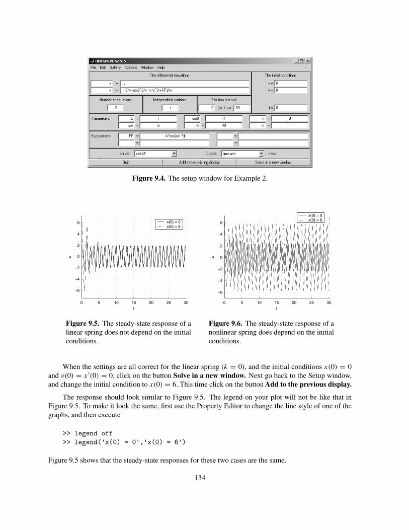
Figure 9.4. The setup window for Example 2.

x

0 5 10 15 20 25 30

−6

−4

−2

0

2

4

6

t

x

x(0) = 0x(0) = 6

x(0) = 0x(0) = 6

0 5 10 15 20 25 30

−6

−4

−2

0

2

4

6

t

xx(0) = 0x(0) = 6

Figure 9.5. The steady-state response of alinear spring does not depend on the initialconditions.

Figure 9.6. The steady-state response of anonlinear spring does depend on the initialconditions.

When the settings are all correct for the linear spring (k = 0), and the initial conditions x(0) = 0and v(0) = x′(0) = 0, click on the button Solve in a new window. Next go back to the Setup window,and change the initial condition to x(0) = 6. This time click on the button Add to the previous display.

The response should look similar to Figure 9.5. The legend on your plot will not be like that inFigure 9.5. To make it look the same, first use the Property Editor to change the line style of one of thegraphs, and then execute

>> legend off>> legend('x(0) = 0','x(0) = 6')

Figure 9.5 shows that the steady-state responses for these two cases are the same.

134

Return to the setup window and change the parameter k to 1 to introduce the nonlinearity. Then resetthe initial condition to x = 0, and repeat the steps. The result is shown in Figure 9.6. The steady-stateresponses are clearly different. This is another way in which nonlinear systems behave differently fromlinear systems.

The Gallery menu contains several interesting systems. Experiment with these to learn more abouthow odesolve works. If you are wondering about stiff equations, choose the 1D stiff example. Try tosolve using ode45. Click the Stop button when you are tired of waiting. Then solve using ode15s.

Options in ODESOLVE

If you find it difficult to see where a solution curve starts, choose the option to mark initial points.You can also choose to mark all of the points computed by the solver.

Since odesolve has a limited number of output possibilities, it will sometimes be necessary to haveaccess to the solution data. There are two ways of doing this using odesolve. First, you can computea solution using odesolve and export the data to the command window workspace. The data in thecommand window will be a structure with the name odedata*, where * is a small number chosen to notconflict with previously saved data. The structure will have a field for each variable. (See Exercises 9and 10.)

The second method is to export an ODE function M-file, which can be used with any of MATLAB’ssolvers to find numerical solutions. If you choose this option, you will be asked for a filename. If youthen execute help on this file, you will be given instructions on how to use a solver with this file.

There will be times when you will want to give a solver a smaller tolerance, or change some othersolver setting. This is possible in odesolve by selecting Options→Solver settings. In this windowit is possible to change settings for the solvers which we have not discussed in this chapter. Read theMATLAB documentation for the definitions.

Finally, odesolve has the capability to save and load systems and whole galleries. These optionsare accessed from the File menu. They work like the same options in dfield and pplane.

Exercises

Most of these exercises are of an advanced nature. However, any of the exercises from Chapter 8 may be done usingodesolve, so look there for more elementary exercises.

1. Revisit Example 1, but do a 2D phase plot, plotting the position of the second mass versus the position ofthe first mass (y versus x). Extend the time period and replot. Do you think the solution is periodic?

2. Plot the solution of x ′′′ + xx ′′/50 = cos t , x(0) = 1, x ′(0) = −1, x ′′(0) = 0 over the time interval [0, 30].

3. Plot the solution of x ′′′′ +x ′′ +x = cos t , x(0) = 1, x ′(0) = −1, x ′′(0) = 0, x ′′′(0) = 0 over the time interval[0, 25]. What happens to the solution if you extend the time interval?

4. A salt solution containing 2 pounds of salt per gallon of water enters a tank at a rate of 4 gal/min. Salt solutionleaves the tank at a rate of 2 gal/min. Initially, the tank contains 10 gallons of pure water. Find the amountof salt in the tank when the volume of solution in the tank reaches 30 gallons. One way to do this problem isto note that the volume of solution in the tank is given by V = 2t + 10 and the salt content is governed bythe differential equation x ′ = 8 − 2x/V , with initial condition x(0) = 0. Set V = 30 in V = 2t + 10 andfind the time. Then solve the initial value problem and substitute this time to get the salt content. However,

135

odesolve offers another method. Set up the system

dx

dt= 8 − 2x

V

dV

dt= 2.

Use a time plot to plot both x and V versus t for the solution with initial conditions x(0) = 0 and V (0) = 10.Examine the plot to determine when V = 30 and note the time when this occurs, then estimate the salt contentfrom the plot at this time.

5. Initially, tank A contains 20 gallons of salt solution, while tanks B and C contain 40 and 50 gallons of purewater, respectively. Pure water enters tank A at a rate of 5 gal/min. Salt solution leaves tank A at a rate of 5gal/min, emptying into tank B at the same rate. In turn, salt solution leaves tank B at 5 gal/min, emptying intotank C at the same rate. Finally, salt solution leaves tank C at 5 gal/min. Because of the constant flow to andfrom each tank, the volume of solution in each tank remains constant for all time. Tank A initially contains15 pounds of salt. Use odesolve to estimate the times when the salt content reaches a maximum in tanks Band C.

6. A driven RC-circuit is modeled with the initial value problem

V ′C = −VC + cos(2πf t), VC(0) = 0,

where f is the frequency of the driving force. For purposes of this demonstration, think of the driving forceVI = cos(2πf t) as the input signal and VC , the voltage response across the capacitor, as the output signal.This circuit is called a low-pass filter. The goal of this problem is to vary the frequency of the input signal andmeasure the response of the circuit by directly comparing the output and input signals. We can get odesolveto do this for us with a little subterfuge. If we differentiate the input signal we get V ′

I = −2πf sin(2πf t).We add this equation to the equation for the circuit to create the system

V ′C = −VC + VI ,

V ′I = −2πf sin(2πf t)

.

Note that we want VI (0) = cos(2πf (0)) = 1. We will have odesolve solve the system, and plot the inputand output signals on the same figure, allowing easy comparison.

a) Set the frequency to f = 0.04 Hz. Recall that the period and frequency are related by T = 1/f , sothe period in this case is T = 25 seconds. Enter the system in odesolve, set the initial conditions toVC(0) = 0 and VI (0) = 1, and enter the parameter f = 0.04. We want to solve over five periods, soset the solution interval to [0, 5T ] = [0, 5/f ]. Solve and plot both VC and VI . How severely, if at all,is the output signal attenuated (reduced in amplitude) in comparison to the input signal?

b) Gradually increase the frequency of the input signal from f = 0.04 Hz to f = 1 Hz, adjusting thesolution interval in each case to [0, 5T ] = [0, 5/f ], graphing the input and output signal over fiveperiods of the input signal.

c) Describe what happens to the amplitude of the output signal in comparison to the input signal as youincrease the frequency of the input signal VI ? Why is this circuit called a low-pass filter?

7. A driven LRC-circuit is modelled by the equation LQ′′ + RQ′ + Q/C = E, where Q is the charge on thecapacitor, L is the inductance, R the resistance, C the capacitance, and E is the driving term, our input voltagein this case. We consider E to be the input signal, and we will measure the output by measuring Q. We willuse odesolve to compare the input and output graphically.

By introducing the current I = Q′, the second order differential equation becomes a system of two firstorder equations, Q′ = I , I ′ = −RI/L − Q/(LC) + E/L. We will use the complicated input E =− cos t − (4/5) cos 5t . Differentiating E we get the three dimensional system

Q′ = I

I ′ = −R

LI − 1

LCQ + 1

LE

E′ = sin t + 4 sin 5t.

136

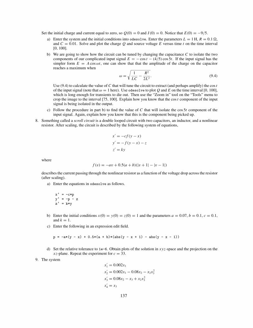
Set the initial charge and current equal to zero, so Q(0) = 0 and I (0) = 0. Notice that E(0) = −9/5.

a) Enter the system and the initial conditions into odesolve. Enter the parameters L = 1 H, R = 0.1 �,and C = 0.01. Solve and plot the charge Q and source voltage E versus time t on the time interval[0, 100].

b) We are going to show how the circuit can be tuned by changing the capacitance C to isolate the twocomponents of our complicated input signal E = − cos t − (4/5) cos 5t . If the input signal has thesimpler form E = A cos ωt , one can show that that the amplitude of the charge on the capacitorreaches a maximum when

ω =√

1

LC− R2

2L2. (9.4)

Use (9.4) to calculate the value of C that will tune the circuit to extract (and perhaps amplify) the cos tof the input signal (note that ω = 1 here). Use odesolve to plot Q and E on the time interval [0, 100],which is long enough for transients to die out. Then use the “Zoom in” tool on the “Tools” menu tocrop the image to the interval [75, 100]. Explain how you know that the cos t component of the inputsignal is being isolated in the output.

c) Follow the procedure in part b) to find the value of C that will isolate the cos 5t component of theinput signal. Again, explain how you know that this is the component being picked up.

8. Something called a scroll circuit is a double looped circuit with two capacitors, an inductor, and a nonlinearresistor. After scaling, the circuit is described by the following system of equations,

x ′ = −cf (y − x)

y ′ = −f (y − x) − z

z′ = ky

wheref (v) = −av + 0.5(a + b)(|v + 1| − |v − 1|)

describes the current passing through the nonlinear resistor as a function of the voltage drop across the resistor(after scaling).

a) Enter the equations in odesolve as follows.

x' = -c*p

y' = -p - z

z' = k*y

b) Enter the initial conditions x(0) = y(0) = z(0) = 1 and the parameters a = 0.07, b = 0.1, c = 0.1,and k = 1.

c) Enter the following in an expression edit field.

p = -a*(y - x) + 0.5*(a + b)*(abs(y - x + 1) - abs(y - x - 1))

d) Set the relative tolerance to 1e-6. Obtain plots of the solution in xyz-space and the projection on thexz-plane. Repeat the experiment for c = 33.

9. The systemx ′

1 = 0.002x1

x ′2 = 0.002x1 − 0.08x2 − x2x

23

x ′3 = 0.08x2 − x3 + x2x

23

x ′4 = x3

137

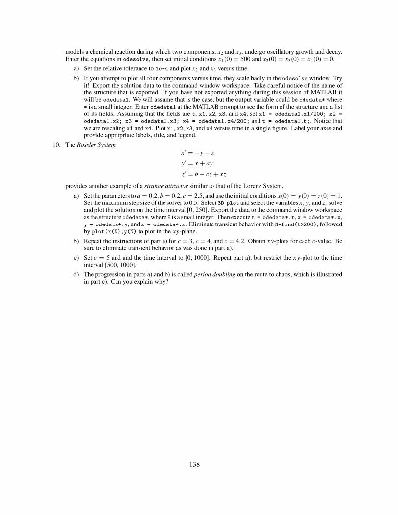
models a chemical reaction during which two components, x2 and x3, undergo oscillatory growth and decay.Enter the equations in odesolve, then set initial conditions x1(0) = 500 and x2(0) = x3(0) = x4(0) = 0.

a) Set the relative tolerance to 1e-4 and plot x2 and x3 versus time.

b) If you attempt to plot all four components versus time, they scale badly in the odesolve window. Tryit! Export the solution data to the command window workspace. Take careful notice of the name ofthe structure that is exported. If you have not exported anything during this session of MATLAB itwill be odedata1. We will assume that is the case, but the output variable could be odedata* where* is a small integer. Enter odedata1 at the MATLAB prompt to see the form of the structure and a listof its fields. Assuming that the fields are t, x1, x2, x3, and x4, set x1 = odedata1.x1/200; x2 =

odedata1.x2; x3 = odedata1.x3; x4 = odedata1.x4/200; and t = odedata1.t;. Notice thatwe are rescaling x1 and x4. Plot x1, x2, x3, and x4 versus time in a single figure. Label your axes andprovide appropriate labels, title, and legend.

10. The Rossler Systemx ′ = −y − z

y ′ = x + ay

z′ = b − cz + xz

provides another example of a strange attractor similar to that of the Lorenz System.

a) Set the parameters to a = 0.2, b = 0.2, c = 2.5, and use the initial conditions x(0) = y(0) = z(0) = 1.Set the maximum step size of the solver to 0.5. Select 3D plot and select the variables x, y, and z. solveand plot the solution on the time interval [0, 250]. Export the data to the command window workspaceas the structure odedata*, where 8 is a small integer. Then execute t = odedata*.t, x = odedata*.x,y = odedata*.y, and z = odedata*.z. Eliminate transient behavior with N=find(t>200), followedby plot(x(N),y(N) to plot in the xy-plane.

b) Repeat the instructions of part a) for c = 3, c = 4, and c = 4.2. Obtain xy-plots for each c-value. Besure to eliminate transient behavior as was done in part a).

c) Set c = 5 and and the time interval to [0, 1000]. Repeat part a), but restrict the xy-plot to the timeinterval [500, 1000].

d) The progression in parts a) and b) is called period doubling on the route to chaos, which is illustratedin part c). Can you explain why?

138

10. The Symbolic Toolbox

The Symbolic Toolbox provides a link between MATLAB and the symbolic algebra program knownas Maple. Unlike the rest of MATLAB, which provides powerful numerical routines, the SymbolicToolbox deals with symbols, formulas, and equations. In dealing with differential equations, it leads toexplicit formulas for the solutions, provided such formulas exist at all.

The Symbolic Toolbox is included with the Student Edition of MATLAB, however, it is distributedas an additional toolbox in the standard version of MATLAB. Therefore it may not be available on yourcomputer. If you are unsure whether or not it is available, execute the command help symbolic atthe MATLAB prompt. If the Symbolic Toolbox is available, you will get a list of all of the commandsavailable in the toolbox. If it is not, you will get an error message, saying symbolic not found.

In this chapter, we will put our emphasis on using the Symbolic Toolbox to solve differentialequations. This means that MATLAB will try to tell you the exact, analytic solution to an equation, oreven to an initial value problem. MATLAB can be successful, of course, only if such a solution exists.To learn more about the Symbolic Toolbox select Help→MATLAB Help from the command windowmenu, and look for the Symbolic Math Toolbox.

Finally, a disclaimer. We are using version 3.0.1 of the Symbolic Toolbox, the latest version availableat the time of this writing. The Symbolic Toolbox has gone through a number of changes recently. Ifyou are not using this version you may notice some differences in the responses to commands. In factwe have noticed different responses from version 3.0.1 operating on different computers. None of thedifferences should be serious, however.

Algebraic Expressions and Symbolic Objects

We have already seen at least three classes of objects in MATLAB. Any numerical quantity, be it anumber or a matrix, is an object of the class double. In addition, we have used strings, which are objectsof class char, and function handles, which are objects in the class function_handle.. The SymbolicToolbox uses algebraic expressions, which are objects of class sym.1 For example, the commands

>> clear all, x = 5; str = 'hello world'; ods = @ode45; y = sym('alpha');

will clear all previously defined variables, and then create four new objects. The object x is an array ofclass double with value 5, str is a string of class char, ods is a function handle, and y is an object ofclass sym with value alpha. The whos command reveals the class of objects in your workspace.

>> whosName Size Bytes Class

ods 1x1 16 function_handle arraystr 1x11 22 char array

1 There are several more classes defined within MATLAB. To see a partial list, execute help class.It is even possible to define your own. For a detailed account of object-oriented programming see Classesand Objects in the online MATLAB documentation.

139

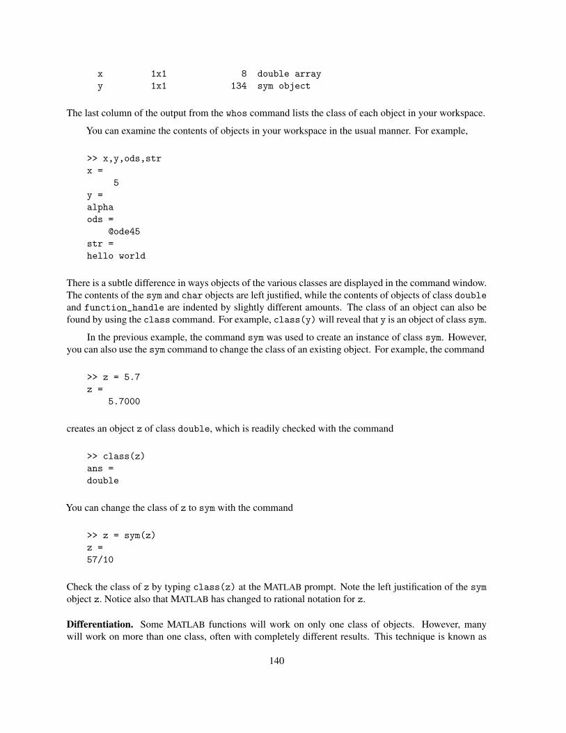
x 1x1 8 double arrayy 1x1 134 sym object

The last column of the output from the whos command lists the class of each object in your workspace.

You can examine the contents of objects in your workspace in the usual manner. For example,

>> x,y,ods,strx =

5y =alphaods =

@ode45str =hello world

There is a subtle difference in ways objects of the various classes are displayed in the command window.The contents of the sym and char objects are left justified, while the contents of objects of class doubleand function_handle are indented by slightly different amounts. The class of an object can also befound by using the class command. For example, class(y) will reveal that y is an object of class sym.

In the previous example, the command sym was used to create an instance of class sym. However,you can also use the sym command to change the class of an existing object. For example, the command

>> z = 5.7z =

5.7000

creates an object z of class double, which is readily checked with the command

>> class(z)ans =double

You can change the class of z to sym with the command

>> z = sym(z)z =57/10

Check the class of z by typing class(z) at the MATLAB prompt. Note the left justification of the symobject z. Notice also that MATLAB has changed to rational notation for z.

Differentiation. Some MATLAB functions will work on only one class of objects. However, manywill work on more than one class, often with completely different results. This technique is known as

140

overloading the function. For example, if you execute help diff, you will discover that diff operateson a vector of class double by taking differences of consecutive elements of the vector. For example:

>> x = [1 2 4 7 11]x =

1 2 4 7 11>> diff(x)ans =

1 2 3 4

The function diff has been overloaded to differentiate objects of class sym. For example:

>> g = sym('x^2')g =x^2>> diff(g)ans =2*x

In this case, MATLAB recognizes that the input argument has class sym and promptly takes the derivativeof g = x2 with respect to x. You will have noticed that the help diff command gives no hint of thisnew power of the function diff until the last few lines, where it lists the overloaded methods. To see adescription of this overloaded method it is necessary to indicate that you want to see how diff works onobjects of class sym. This is done with the command help sym/diff. Try it!

You can declare symbolic objects one at a time, such as

>> x = sym('x'); a = sym('a'); b = sym('b'); c = sym('c');

or you can use the syms command to declare them all at once, as in

>> syms x a b c

The order of declaration is unimportant.

The operators +, -, *, /, and ^ have overloaded definitions for use on symbolic objects, so you canuse them to create algebraic expressions. For example, since a, b, c, and x have been declared to besymbolic objects,

>> f = a^2*x^2 + b*x + c;

creates a new symbolic object f. We can compute the derivative of f with the command

>> diff(f)ans =2*a^2*x+b

We can just as easily take a second derivative.

>> diff(f,2)ans =2*a^2

141

The default variable. How did the Symbolic Toolbox know to differentiate with respect to x, and notwith respect to another symbolic variable, say a? The answer lies in the Symbolic Toolbox’s defaultvariable:

The default symbolic variable in a symbolic expression is the variable that is closest to ‘x’alphabetically.

The findsym command will find all of the symbolic variables in a symbolic expression.

>> findsym(f)ans =a, b, c, x

The command findsym(f,n) returns the n symbolic variables which are closest to x in the alphabet.Hence,

>> findsym(f,1)ans =x

returns the default symbolic variable. That is why the Symbolic Toolbox differentiated with respect tox in the above example. Of course, most Symbolic Toolbox commands allow the user to override thedefault symbolic variable. For example,

>> diff(f,a)ans =2*a*x^2

finds the derivative of f with respect to a, and

>> diff(f,a,2)ans =2*x^2

finds the second derivative of f with respect to a.

Verifying Solutions to Differential Equations

After having completed extensive paper and pencil work to obtain the solution of a differentialequation or initial value problem, you might want to check your answer. Why not let the SymbolicToolbox do the work for you?

Example 1. Verify that y(t) = ce−t2is a solution of

y′ + 2ty = 0, (10.1)

where c is an arbitrary constant.

142

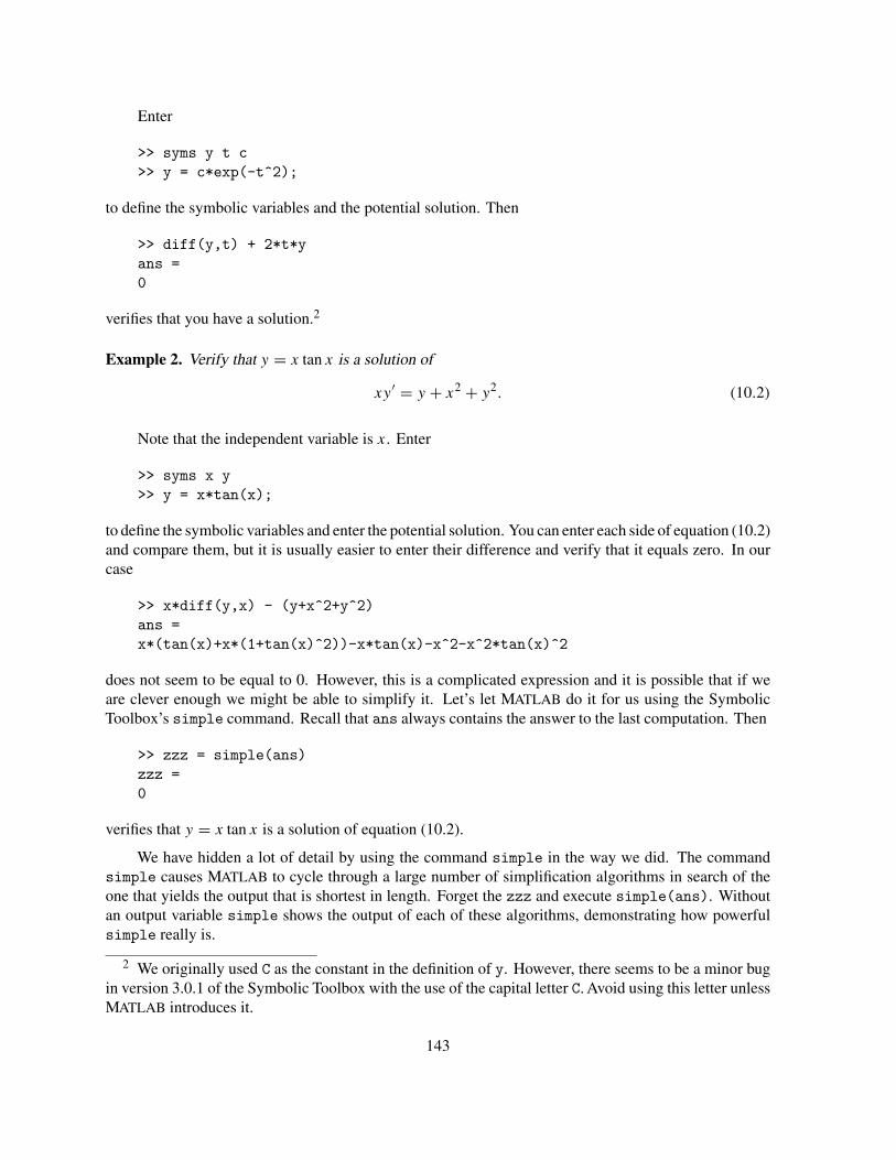
Enter

>> syms y t c>> y = c*exp(-t^2);

to define the symbolic variables and the potential solution. Then

>> diff(y,t) + 2*t*yans =0

verifies that you have a solution.2

Example 2. Verify that y = x tan x is a solution of

xy′ = y + x2 + y2. (10.2)

Note that the independent variable is x. Enter

>> syms x y>> y = x*tan(x);

to define the symbolic variables and enter the potential solution. You can enter each side of equation (10.2)and compare them, but it is usually easier to enter their difference and verify that it equals zero. In ourcase

>> x*diff(y,x) - (y+x^2+y^2)ans =x*(tan(x)+x*(1+tan(x)^2))-x*tan(x)-x^2-x^2*tan(x)^2

does not seem to be equal to 0. However, this is a complicated expression and it is possible that if weare clever enough we might be able to simplify it. Let’s let MATLAB do it for us using the SymbolicToolbox’s simple command. Recall that ans always contains the answer to the last computation. Then

>> zzz = simple(ans)zzz =0

verifies that y = x tan x is a solution of equation (10.2).

We have hidden a lot of detail by using the command simple in the way we did. The commandsimple causes MATLAB to cycle through a large number of simplification algorithms in search of theone that yields the output that is shortest in length. Forget the zzz and execute simple(ans). Withoutan output variable simple shows the output of each of these algorithms, demonstrating how powerfulsimple really is.

2 We originally used C as the constant in the definition of y. However, there seems to be a minor bugin version 3.0.1 of the Symbolic Toolbox with the use of the capital letter C. Avoid using this letter unlessMATLAB introduces it.

143

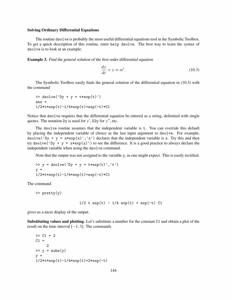
Solving Ordinary Differential Equations

The routine dsolve is probably the most useful differential equations tool in the Symbolic Toolbox.To get a quick description of this routine, enter help dsolve. The best way to learn the syntax ofdsolve is to look at an example.

Example 3. Find the general solution of the first order differential equation

dy

dt+ y = tet . (10.3)

The Symbolic Toolbox easily finds the general solution of the differential equation in (10.3) withthe command

>> dsolve('Dy + y = t*exp(t)')ans =1/2*t*exp(t)-1/4*exp(t)+exp(-t)*C1

Notice that dsolve requires that the differential equation be entered as a string, delimited with singlequotes. The notation Dy is used for y′, D2y for y′′, etc.

The dsolve routine assumes that the independent variable is t. You can override this defaultby placing the independent variable of choice as the last input argument to dsolve. For example,dsolve('Dy + y = x*exp(x)','x') declares that the independent variable is x. Try this and thentry dsolve('Dy + y = x*exp(x)') to see the difference. It is a good practice to always declare theindependent variable when using the dsolve command.

Note that the output was not assigned to the variable y, as one might expect. This is easily rectified.

>> y = dsolve('Dy + y = t*exp(t)','t')y =1/2*t*exp(t)-1/4*exp(t)+exp(-t)*C1

The command

>> pretty(y)

1/2 t exp(t) - 1/4 exp(t) + exp(-t) C1

gives us a nicer display of the output.

Substituting values and plotting. Let’s substitute a number for the constant C1 and obtain a plot of theresult on the time interval [−1, 3]. The commands

>> C1 = 2C1 =

2>> y = subs(y)y =1/2*t*exp(t)-1/4*exp(t)+2*exp(-t)

144

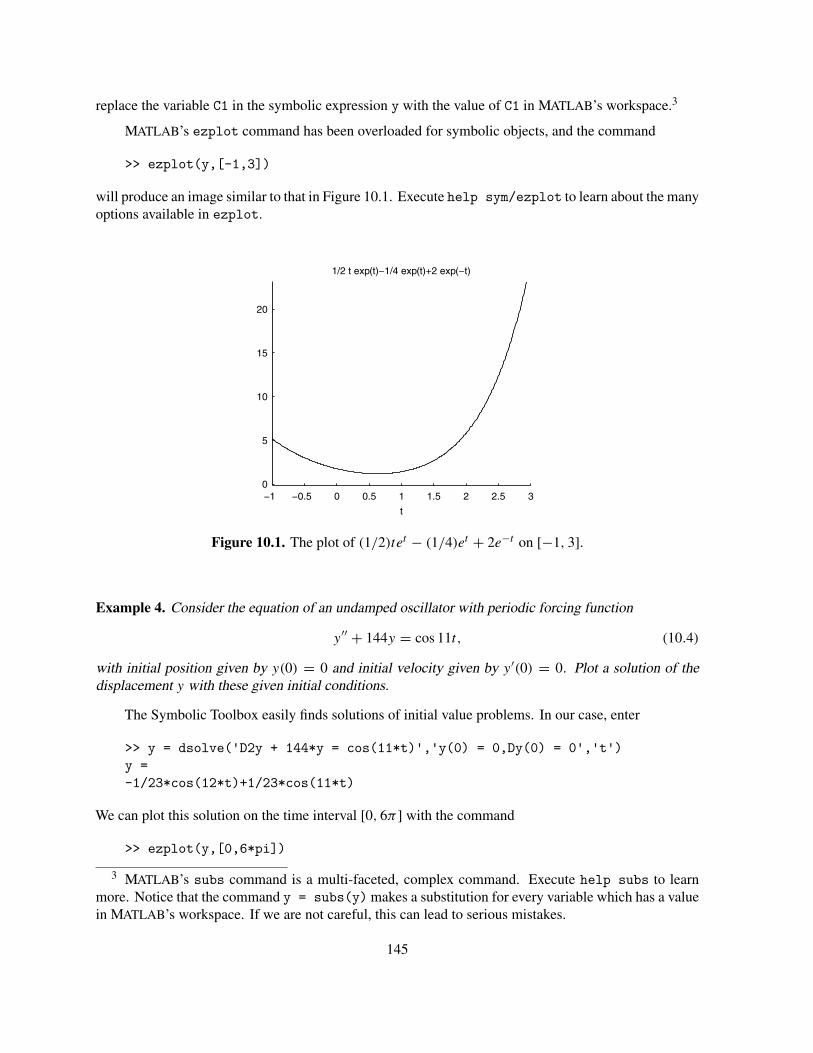
replace the variable C1 in the symbolic expression y with the value of C1 in MATLAB’s workspace.3

MATLAB’s ezplot command has been overloaded for symbolic objects, and the command

>> ezplot(y,[-1,3])

will produce an image similar to that in Figure 10.1. Execute help sym/ezplot to learn about the manyoptions available in ezplot.

−1 −0.5 0 0.5 1 1.5 2 2.5 30

5

10

15

20

t

1/2 t exp(t)−1/4 exp(t)+2 exp(−t)

Figure 10.1. The plot of (1/2)tet − (1/4)et + 2e−t on [−1, 3].

Example 4. Consider the equation of an undamped oscillator with periodic forcing function

y′′ + 144y = cos 11t, (10.4)

with initial position given by y(0) = 0 and initial velocity given by y′(0) = 0. Plot a solution of thedisplacement y with these given initial conditions.

The Symbolic Toolbox easily finds solutions of initial value problems. In our case, enter

>> y = dsolve('D2y + 144*y = cos(11*t)','y(0) = 0,Dy(0) = 0','t')y =-1/23*cos(12*t)+1/23*cos(11*t)

We can plot this solution on the time interval [0, 6π ] with the command

>> ezplot(y,[0,6*pi])

3 MATLAB’s subs command is a multi-faceted, complex command. Execute help subs to learnmore. Notice that the command y = subs(y) makes a substitution for every variable which has a valuein MATLAB’s workspace. If we are not careful, this can lead to serious mistakes.

145

0 5 10 15−0.1

−0.08

−0.06

−0.04

−0.02

0

0.02

0.04

0.06

0.08

t

1/23*cos(11*t)−1/23*cos(12*t)

Figure 10.2. The solution of y′′ + 144y = cos 11t , y(0) = 0, y′(0) = 0.

producing an image similar to that in Figure 10.2. The phenomenon displayed in Figure 10.2 is calledbeats, a condition present in undamped, forced oscillators that are nearly resonant.

Solving Systems of Ordinary Differential Equations

The routine dsolve solves systems of equations almost as easily as it does single equations, as longas there actually is an analytical solution.

Example 5. Find the solution of the initial value problem

x′ = −2x − 3y,

y′ = 3x − 2y,(10.5)

with x(0) = 1 and y(0) = −1.

It is a good idea to clear variables from your workspace when they are no longer needed. Left-overvariables can wreak unexpected havoc when employing the subs command. You can delete all4 variablesfrom your workspace with

>> clear all

Enter the whos command to verify that there are no variables left in the workspace.

We can call dsolve in the usual manner. Readers will note that the input to dsolve in this exampleparallels that in Examples 3 and 4. The difference lies in the output variable(s). If a single variable is used

4 You can also select individual variables for deletion. For example, the command clear t clearsonly the variable t from your workspace.

146

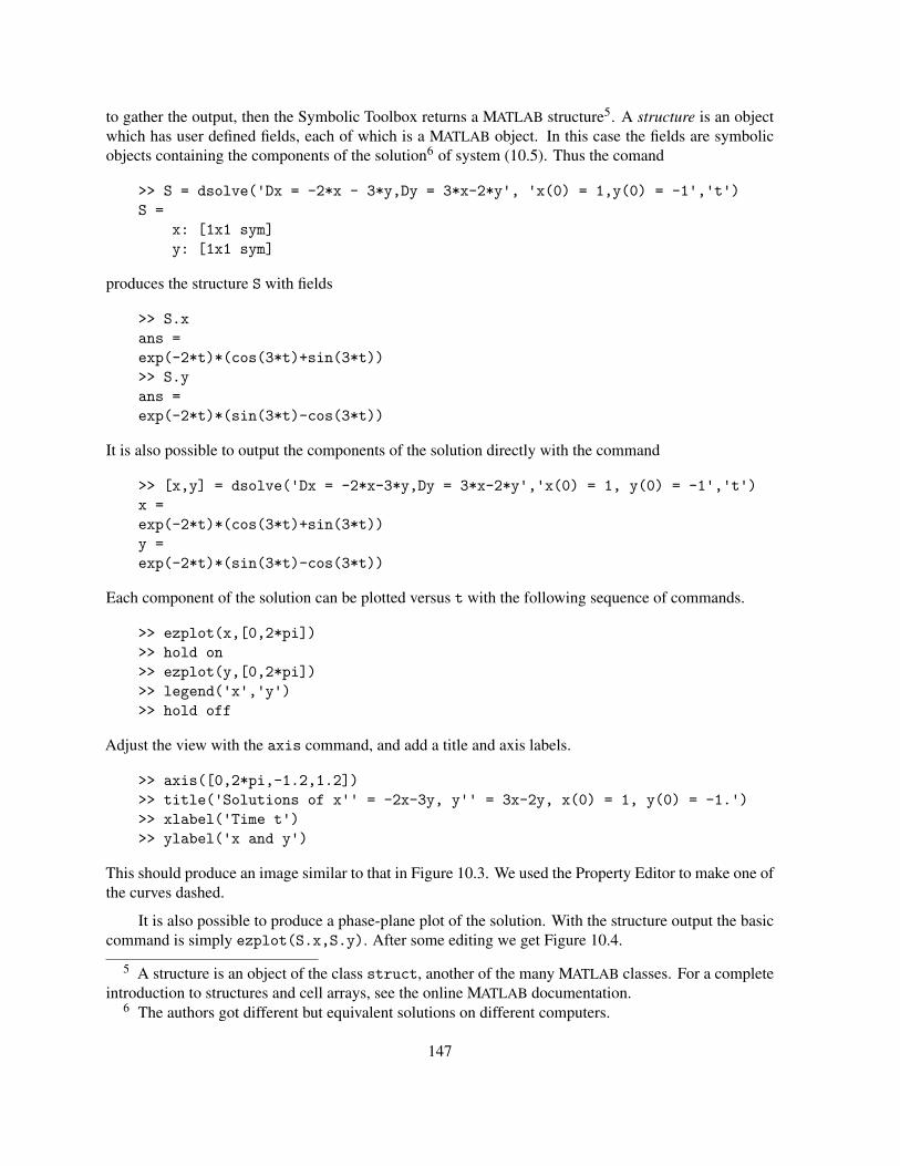
to gather the output, then the Symbolic Toolbox returns a MATLAB structure5. A structure is an objectwhich has user defined fields, each of which is a MATLAB object. In this case the fields are symbolicobjects containing the components of the solution6 of system (10.5). Thus the comand

>> S = dsolve('Dx = -2*x - 3*y,Dy = 3*x-2*y', 'x(0) = 1,y(0) = -1','t')S =

x: [1x1 sym]y: [1x1 sym]

produces the structure S with fields

>> S.xans =exp(-2*t)*(cos(3*t)+sin(3*t))>> S.yans =exp(-2*t)*(sin(3*t)-cos(3*t))

It is also possible to output the components of the solution directly with the command

>> [x,y] = dsolve('Dx = -2*x-3*y,Dy = 3*x-2*y','x(0) = 1, y(0) = -1','t')x =exp(-2*t)*(cos(3*t)+sin(3*t))y =exp(-2*t)*(sin(3*t)-cos(3*t))

Each component of the solution can be plotted versus t with the following sequence of commands.

>> ezplot(x,[0,2*pi])>> hold on>> ezplot(y,[0,2*pi])>> legend('x','y')>> hold off

Adjust the view with the axis command, and add a title and axis labels.

>> axis([0,2*pi,-1.2,1.2])>> title('Solutions of x'' = -2x-3y, y'' = 3x-2y, x(0) = 1, y(0) = -1.')>> xlabel('Time t')>> ylabel('x and y')

This should produce an image similar to that in Figure 10.3. We used the Property Editor to make one ofthe curves dashed.

It is also possible to produce a phase-plane plot of the solution. With the structure output the basiccommand is simply ezplot(S.x,S.y). After some editing we get Figure 10.4.

5 A structure is an object of the class struct, another of the many MATLAB classes. For a completeintroduction to structures and cell arrays, see the online MATLAB documentation.

6 The authors got different but equivalent solutions on different computers.

147

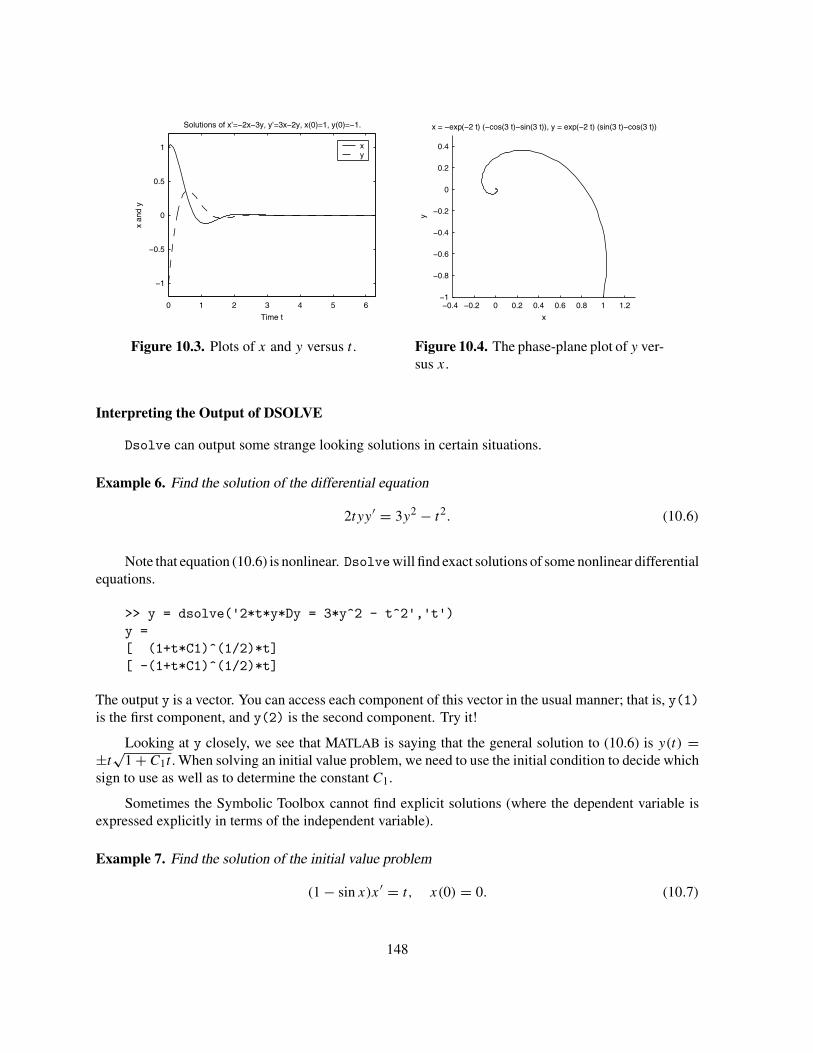
0 1 2 3 4 5 6

−1

−0.5

0

0.5

1

Time t

Solutions of x’=−2x−3y, y’=3x−2y, x(0)=1, y(0)=−1.

x an

d y

xy

−0.4 −0.2 0 0.2 0.4 0.6 0.8 1 1.2−1

−0.8

−0.6

−0.4

−0.2

0

0.2

0.4

x

y

x = −exp(−2 t) (−cos(3 t)−sin(3 t)), y = exp(−2 t) (sin(3 t)−cos(3 t))

Figure 10.3. Plots of x and y versus t . Figure 10.4. The phase-plane plot of y ver-sus x.

Interpreting the Output of DSOLVE

Dsolve can output some strange looking solutions in certain situations.

Example 6. Find the solution of the differential equation

2tyy′ = 3y2 − t2. (10.6)

Note that equation (10.6) is nonlinear. Dsolvewill find exact solutions of some nonlinear differentialequations.

>> y = dsolve('2*t*y*Dy = 3*y^2 - t^2','t')y =[ (1+t*C1)^(1/2)*t][ -(1+t*C1)^(1/2)*t]

The output y is a vector. You can access each component of this vector in the usual manner; that is, y(1)is the first component, and y(2) is the second component. Try it!

Looking at y closely, we see that MATLAB is saying that the general solution to (10.6) is y(t) =±t

√1 + C1t . When solving an initial value problem, we need to use the initial condition to decide which

sign to use as well as to determine the constant C1.

Sometimes the Symbolic Toolbox cannot find explicit solutions (where the dependent variable isexpressed explicitly in terms of the independent variable).

Example 7. Find the solution of the initial value problem

(1 − sin x)x′ = t, x(0) = 0. (10.7)

148

Equation (10.7) is separable. The general solution is given by the implicit formula

x + cos x = t2

2+ 1. (10.8)

Of course, it is not possible to solve equation (10.8) for x in terms of t . When we execute

>> dsolve('(1 - sin(x))*Dx = t', 'x(0) = 0','t')

to see what MATLAB will do, we get an error message saying that MATLAB will not look for implicitsolutions when initial conditions are given. So we execute

>> dsolve('(1 - sin(x))*Dx = t','t')Warning: Explicit solution could not be found; implicit solution returned.> In C:\MATLAB6p5\toolbox\symbolic\dsolve.m at line 292ans =1/2*t^2-x-cos(x)+C1 = 0

This time, MATLAB tells us that it could not find an explicit solution and gives us the formula for thegeneral implicit solution. We can find out what the constant has to be by using the initial conditions andthe subs command.

>> x = 0; t = 0;>> subs(ans)ans =-1+C1 = 0

Thus, C1 = 1 and we see that the solution to the initial value problem satisfies the implicit equation(1/2)t2 − x − cos x + 1 = 0, which is equivlalent to (10.8).7

The Solve Command

The solve command is the Symbolic Toolbox’s versatile equation solver. It performs equally wellwith single equations and multiple equations. For example, if you need to solve the equation ax +b = 0,then the command

>> solve('a*x + b')ans =-b/a

provides the solution, x = −b/a. We need to make two important points about the syntax of the solvecommand. First, the command solve('a*x+b') is identical to the command solve('a*x+b=0'). Try

7 Different versions of the Symbolic Toolbox give quite different responses when implicitly definedsolutions appear.

149

it! Second, we did not indicate what variable to solve for, so the solve command found a solution forthe default variable.8 You can choose a different solution variable. The command

>> solve('a*x+b','a')ans =-b/x

solves the equation ax + b = 0 for a.

If an equation has multiple solutions, they are listed in an output vector.

>> s = solve('a*x^2 + b*x + c')s =[ 1/2/a*(-b+(b^2-4*a*c)^(1/2))][ 1/2/a*(-b-(b^2-4*a*c)^(1/2))]

You can access the components of the solution vector in the usual manner.

The command

>> pretty(s(1))2 1/2

-b + (b - 4 a c)1/2 --------------------

a

will display the formula in more understandable form.

Finally, if the Symbolic Toolbox cannot find a symbolic solution, it will attempt to find a numericalsolution.

>> s = solve('x + 2 = exp(x^2)')s =1.0571035499947380777922377221533

That’s 32 significant figures. If you want more, say 40, execute

>> digits(40)>> s = solve('x+2 = exp(x^2)')s =1.057103549994738077792237722153280429451

Example 8. The logistic model for population growth is given by the equation

dp

dt= k

(

1 − P

N

)

P, (10.9)

where k is the natural growth rate of the population and N is the carrying capacity of the environment.Assume that k = 0.025 and N = 1000. How long will it take an initial population of 200 to grow to800? Assume that time is measured in minutes.

8 Type findsym(sym(’a*x+b’),1) to find the default variable in the expression ax + b.

150

With k = 0.025 and N = 1000, equation (10.9) becomes dP/dt = 0.025(1 − P/1000)P , withinitial population given by P(0) = 200. Using dsolve,

>> P = dsolve('DP = 0.025*(1-P/1000)*P','P(0) = 200','t')P =1000/(1+4*exp(-1/40*t))

we find that the solution of the initial value problem is

P = 1000

1 + 4e−t/40 . (10.10)

The following commands provide a plot similar to that in Figure 10.5.

>> ezplot(P,[0,300])>> grid>> xlabel('Time in minutes')>> ylabel('Population')>> title('A Logistic Model')

0 50 100 150 200 250 300

200

300

400

500

600

700

800

900

1000

Time in minutes

A Logistic Model

Pop

ulat

ion

Figure 10.5. The solution of dP/dt = 0.025(1 − P/1000)P , P(0) = 200.

If you examine the plot in Figure 10.5, it appears that the population reaches a level of 800 somewherebetween 100 and 150 minutes. Substituting P = 800 in equation (10.10), we see that we want to find t

so that

800 = 1000

1 + 4e−t/40 .

151

For this we can use the commands9

>> s = solve('800 = 1000/(1+4*exp(-t/40))','t')s =40*log(16)>> double(s)ans =110.9035

Consequently, it takes approximately 111 minutes for the population to reach 800.

Exercises

In Exercises 1 – 5, use MATLAB and the technique demonstrated in Examples 1 and 2 to verify that y is a solutionto the indicated equation.

1. y = 1 + e−t2/2, y ′ + ty = t .

2. w = 1/(s − 3), w′ + w2 = 0.

3. y = 10 − t2/2, yy ′ + ty = 0.

4. y = ln(x), (2ey − x)y ′ = 1. Recall: ln(x) is log(x) in MATLAB.

5. y = et cos(2t), y ′′ − 2y ′ + 5y = 0.

In Exercises 6 – 11, determine the independent variable, and use dsolve to find the general solution to the indicatedequation. Use the subs command to replace the integration constant C1with C1 = 2. Use ezplot to plot the resultingsolution.

6. y ′ + ty = t .

7. y ′ + y2 = 0.

8. yy ′ + ty = 0.

9. (2ey − x)y ′ = 1. Hint: Use dsolve('(2*exp(y)-x)*Dy = 1','x').

10. (x + y2)y ′ = y.

11. x(y ′ − y) = ex .

In Exercises 12 – 17, determine the independent variable, and use dsolve to find the solution to the indicated initialvalue problem. Use ezplot to plot the solution over the indicated time interval.

12. y ′ + ty = t , y(0) = −1, [−4, 4].

13. y ′ + y2 = 0, y(0) = 2, [0, 5].

14. yy ′ + ty = 0, y(1) = 4, [−4, 4].

15. (2ey − x)y ′ = 1, y(0) = 0, [−5, 5]. Hint: dsolve('(2*exp(y)-x)*Dy=1','y(0)=0','x').

16. (x + y2)y ′ = y, y(0) = 4, [−4, 6].

17. x(y ′ − y) = ex , y(1) = 4e, [0.0001, 0.001], and [0.001, 1].

In Exercises 18 and 19, use dsolve to obtain the solution of each of the indicated second order differential equations.Use the simple command to find the simplest form of that solution. Use ezplot to sketch the solution on theindicated time interval.

9 You can actually get pretty fancy here and enter solve(P-800). This is pretty sophisticated use ofthe Symbolic Toolbox, and indicates some of the power you can attain with experience.

152

18. y ′′ + 4y = 3 cos 2.1ty(0) = 0, y ′(0) = 0, [0, 64π ]

19. y ′′ + 16y = 3 sin 4ty(0) = 0, y ′(0) = 0, [0, 32π ]

20. Use dsolve to obtain the solution of y ′′ + y ′ + 144y = cos 2t , y(0) = 0, y ′(0) = 0. Use ezplot to plot thesolution on the time interval [0, 6π ]. Use ode45 to find a numerical solution on the same time interval andsuperimpose that plot of the first plot. How closely does the numerical solution match the symbolic solution?

21. Use the technique of Examples 1 and 2 to verify that

x = e−t (cos 2t − sin 2t),

y = e−t (3 sin 2t − cos 2t),

is a solution of the systemx ′ = −5x − 2y,

y ′ = 10x + 3y.

Furthermore, use the subs command to verify that the solution satisfies the initial conditions x(0) = 1 andy(0) = −1.

22. Use dsolve to solve the initial value problem

y ′ = v,

v′ = −2v − 2y + cos 2t,

with y(0) = 1 and v(0) = −1, over the time interval [0, 30].

In Exercises 23 – 25, find the solutions to the indicated initial value problem.

23. t2y ′′ = (y ′)2, with y(1) = 3 and y ′(1) = 2.

24. y ′′ = yy ′, with y(0) = 0, and y ′(0) = 2.

25. y ′′ = ty ′ + y + 1, with y(0) = 1, and y ′(0) = 0.

26. Suppose we start with a population of 100 individuals at time t = 0, and that the population is correctlymodeled by the logistic equation. Suppose that at time t = 2 there are 200 individuals in the population,and that the population approaches steady state at a population of 1000. Plot the population over the interval[0, 20]. What is the population at time t = 10?

27. Suppose we have a population which is correctly modeled by the logistic equation, and experimental mea-surements show that p(0) = 50, p(1) = 150, and p(2) = 250. Use the Symbolic Toolbox to derive theformula for the population as a function of time. Plot the population over the interval [0, 5]. What is thelimiting value of the population? What is p(3)?

153

11. Linear Algebra Using MATLAB

MATLAB is short for “Matrix Laboratory.” It contains a large number of built-in routines that makematrix algebra very easy. In this chapter we will learn how to use some of those routines to solve systemsof linear equations. In the next chapter we will use the linear algebra learned here to help us solve systemsof differential equations.

Systems of Linear Equations

Let’s start by looking at a very elementary example.

Example 1. Find the solution to the system

u + 2v = 5,

4u − v = 2.(11.1)

Using the method usually taught in secondary school, we solve the first equation for the variable u,yielding u = 5 − 2v, and substitute this result into the second equation. In this way we obtain a newsystem consisting of the first equation and the modified second equation

u + 2v = 5,

−9v = −18,(11.2)

which has the same solutions as (11.1). The advantage is that the variable u has been eliminated from thesecond equation. Therefore, system (11.2) is quite easily solved by the method known as backsolving.This means that we solve the system by starting with the last equation and move up. From the secondequation in (11.2), we see that v = 2. Substituting v = 2 into the first equation, we can solve for u,getting u = 1.

The system in (11.1) is a system of two equations with two unknowns. We want to find a systematicmethod that will work in general for m equations involving n unknowns, where m, and n are possiblyvery large, and not necessarily equal. Our goal is to find all solutions of such a system. The generalmethod is not significantly different from the method of elimination and backsolving used in Example 1.

Linear Combinations of Vectors and the Matrix-Vector Product

We need to develop some algebraic ideas to facilitate our solution method. We can put both sidesof equation (11.1) into vectors, so that it reads

[

u + 2v

4u − v

]

=[

52

]

. (11.3)

Using standard arithmetic operations with vectors, we can rewrite the left-hand side so that (11.3) becomes

u

[

14

]

+ v

[

2−1

]

=[

52

]

. (11.4)

154

The form of the left-hand side in (11.4) is so important we give it a name. It is called the linearcombination of the vectors [1, 4]T and [2, −1]T with coefficients u and v. In general, let v1, v2, . . . , vp

be vectors of the same size, and let x1, x2, . . . , xp be scalars.1 Then

x1v1 + x2v2 + · · · + xpvp

is called the linear combination of the vectors v1, v2, . . . , vp with coefficients x1, x2, . . . , xp. With thisnew terminology, the problem of solving the system in (11.1) becomes that of finding the coefficients u

and v so that the linear combination with these coefficients is equal to the right-hand side in (11.4).

The concept of linear combination, together with its importance in understanding systems of equa-tions as indicated in equation (11.4), leads us to the definition of matrix-vector multiplication. We formallydefine the product of a matrix A and a vector x to be the vector Ax which is the linear combination ofthe columns of A, using the entries of the vector x for the scalars in the linear combination. Thus, if A

is the matrix which has the vectors v1, v2, . . . , vp as columns and x = [x1, x2, . . . , xp]T , then

Ax = x1v1 + x2v2 + · · · + xpvp.

Let’s return to the system in (11.1). We reinterpreted the system as a linear combination in (11.4).In view of the definition of matrix-vector product, we can write (11.4) as

[

1 24 −1

] [

u

v

]

=[

52

]

. (11.5)

If we define

A =[

1 24 −1

]

, x =[

u

v

]

, and b =[

52

]

, (11.6)

the system of equations can be written as Ax = b. If we compare equations (11.5) and (11.6) to theoriginal system in (11.1) we see that the matrix A contains the coefficients of the system. It is thereforecalled the coefficient matrix. Similarly, the vector b is called the right-hand side and the vector x is calledthe vector of unknowns or the unknown vector.

Let’s look at the concepts of linear combination and matrix multiplication for a more complicatedexample.

Example 2. Consider the vectors

a1 =[ 2

−2−2

]

, a2 =[ 4

34

]

, and a3 =[−3

21

]

.

Form and simplify the linear combination 1a1 + 0a2 − 2a3.

1 Scalars are simply numbers. In most examples here they are real numbers, but they could also becomplex numbers. Indeed, the vectors themselves could have complex entries.

155

This is easily accomplished in MATLAB.

>> a1 = [2;-2;-2]; a2 = [4;3;4]; a3 = [-3;2;1];>> 1*a1 + 0*a2 - 2*a3ans =

8-6-4

Example 3. Find the matrix-vector product Ax, where

A =[ 2 4 −3

−2 3 2−2 4 1

]

and x =[ 1

0−2

]

.

Note that the columns of matrix A are the vectors

a1 =[ 2

−2−2

]

, a2 =[ 4

34

]

, and a3 =[−3

21

]

,

which were used in Example 2. According to the definition, the matrix-vector product is computed byforming a linear combination of the columns of matrix A, using the entries of vector x as the scalars.Note that the vector x has three entries, one for each column of matrix A. Otherwise, the multiplicationwould not be possible. Thus,

Ax =[ 2 4 −3

−2 3 2−2 4 1

][ 10

−2

]

= 1

[ 2−2−2

]

+ 0

[ 434

]

− 2

[−321

]

=[ 8

−6−4

]

To perform this same calculation in MATLAB, we first enter the matrix A. Since we have alreadyentered the column vectors in Example 2, it is easier to create A with the command

>> A = [a1,a2,a3]A =

2 4 -3-2 3 2-2 4 1

Next we enter the vector x = [1, 0, −2]T into MATLAB and perform the multiplication with the commands

>> x = [1;0;-2]; b = A*xb =

8-6-4

156

Notice that this command is simply * and not .*. The operation * is called matrix multiplication, and itis quite different from .*, which is the operation of array multiplication that we studied in Chapter 2.

It is important to notice that the same solution is found in Examples 2 and 3. Realizing that matrix-vector multiplication amounts to taking a linear combination of the columns of the matrix, with the entriesof the vector for the scalars, is the key to recognizing where matrix multiplication can be used to solveproblems.

Let’s use these ideas to solve a system of equations.

Example 4. Solve the following system of equations for x1, x2, and x3.

2x1 + 4x2 − 3x3 = 8

−2x1 + 3x2 + 2x3 = −6

−2x1 + 4x2 + x3 = −4

(11.7)

The three equalities in (11.7) can be written as the single vector equality[ 2x1 + 4x2 − 3x3

−2x1 + 3x2 + 2x3−2x1 + 4x2 + x3

]

=[ 8

−6−4

]

. (11.8)

Standard vector algebra allows us to write the left-hand side of equation (11.8) as the linear combination

x1

[ 2−2−2

]

+ x2

[ 434

]

+ x3

[−321

]

=[ 8

−6−4

]

. (11.9)

Next, we notice that the linear combination on the left-hand side of equation (11.9) can be written as amatrix-vector product, giving us

[ 2 4 −3−2 3 2−2 4 1

][

x1x2x3

]

=[ 8

−6−4

]

. (11.10)

Equation (11.10) is in the form Ax = b, where

A =[ 2 4 −3

−2 3 2−2 4 1

]

and b =[ 8

−6−4

]

.

The matrix A is the same matrix found in Example 3, and it is the coefficient matrix for the systemin (11.7). It is formed by recording the coefficients of x1, x2, and x3 from the system of equations in(11.7). In this case we can solve the equation Ax = b by dividing both sides of the equation on the leftby the matrix A, leading to A\Ax = A\b, or x = A\b. This is easily accomplished in MATLAB. Thematrix A and the vector b were formed in the previous examples, so all we need to do is enter

>> x = A\bx =

10

-2

157

Once again we have demonstrated the ease with which MATLAB can solve mathematical problems.Indeed the method of the previous paragraph works in great generality. However, it does not alwayswork! In order for it to work, it is necessary that the coefficient matrix be nonsingular (the termnonsingular will be defined later in this chapter). Unfortunately, many of the applications of linearsystems to ordinary differential equations have coefficient matrices which are singular. Furthermore,since matrix multiplication is a rather complicated procedure, one can expect that matrix division is atleast equally complicated. The above naive approach is hiding a lot of mathematics as we will soon see.

Matrix Multiplication

Before continuing with our search for a method of solving systems of equations, let’s extend theidea of matrix-vector product to the product of two matrices. The operation of multiplying two matricesis called matrix multiplication. It might seem complicated, but it is easily defined using matrix-vectormultiplication defined earlier, and demonstrated in Example 3.

Suppose that we have two matrices A and B and that the number of columns of A is equal to thenumber of rows of B. Let b1, b2, . . . , bp represent the columns of matrix B. We will denote this by theequation

B = [b1, b2, . . . , bp

]

.

Then the matrix product AB is defined by

AB = A[

b1, b2, . . . , bp

]

,

= [Ab1, Ab2, . . . , Abp

]

.

Therefore, the matrix product AB is formed by multiplying each column of the matrix B by the matrixA.

Example 5. Find the matrix product AB, where

A =[ 1 −1 1

0 1 −21 0 1

]

and B =[ 2 1

2 −22 0

]

.

The first column of the matrix B is

b1 =[ 2

22

]

.

Therefore, the first column of the matrix product AB is Ab1. This multiplication would not be possibleif it were not for the fact that the number of rows of B equals the number of columns of A. We get

Ab1 =[ 1 −1 1

0 1 −21 0 1

][ 222

]

= 2

[ 101

]

+ 2

[−110

]

+ 2

[ 1−2

1

]

=[ 2

−24

]

158

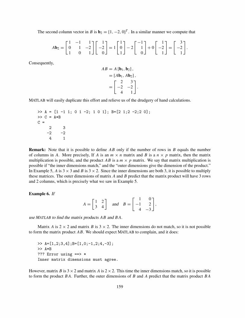
The second column vector in B is b2 = [1, −2, 0]T . In a similar manner we compute that

Ab2 =[ 1 −1 1

0 1 −21 0 1

][ 1−2

0

]

= 1

[ 101

]

− 2

[−110

]

+ 0

[ 1−2

1

]

=[ 3

−21

]

.

Consequently,AB = A [b1, b2] ,

= [Ab1, Ab2] ,

=[ 2 3

−2 −24 1

]

.

MATLAB will easily duplicate this effort and relieve us of the drudgery of hand calculations.

>> A = [1 -1 1; 0 1 -2; 1 0 1]; B=[2 1;2 -2;2 0];>> C = A*BC =

2 3-2 -24 1

Remark: Note that it is possible to define AB only if the number of rows in B equals the numberof columns in A. More precisely, If A is an m × n matrix and B is a n × p matrix, then the matrixmultiplication is possible, and the product AB is a m × p matrix. We say that matrix multiplication ispossible if “the inner dimensions match,” and the “outer dimensions give the dimension of the product.”In Example 5, A is 3 × 3 and B is 3 × 2. Since the inner dimensions are both 3, it is possible to multiplythese matrices. The outer dimensions of matrix A and B predict that the matrix product will have 3 rowsand 2 columns, which is precisely what we saw in Example 5.

Example 6. If

A =[

1 23 4

]

and B =[ 1 0

−1 24 −3

]

,

use MATLAB to find the matrix products AB and BA.

Matrix A is 2 × 2 and matrix B is 3 × 2. The inner dimensions do not match, so it is not possibleto form the matrix product AB. We should expect MATLAB to complain, and it does:

>> A=[1,2;3,4];B=[1,0;-1,2;4,-3];>> A*B??? Error using ==> *Inner matrix dimensions must agree.

However, matrix B is 3 × 2 and matrix A is 2 × 2. This time the inner dimensions match, so it is possibleto form the product BA. Further, the outer dimensions of B and A predict that the matrix product BA

159

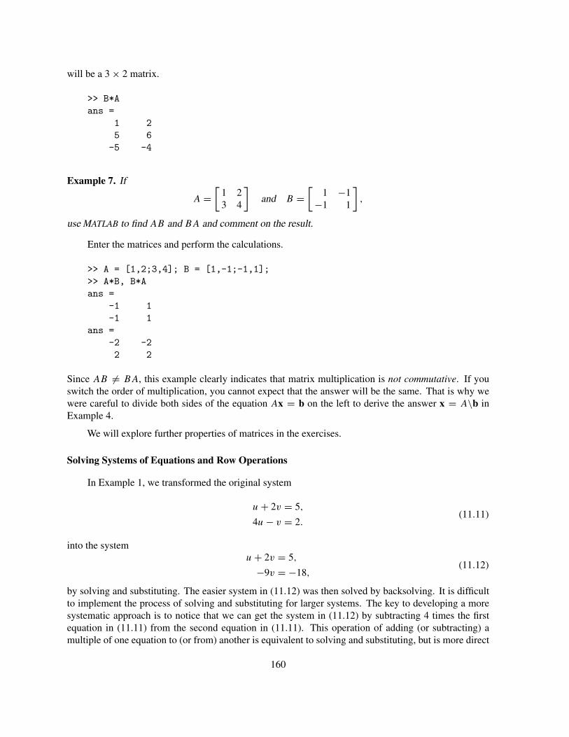
will be a 3 × 2 matrix.

>> B*Aans =

1 25 6

-5 -4

Example 7. If

A =[

1 23 4

]

and B =[

1 −1−1 1

]

,

use MATLAB to find AB and BA and comment on the result.

Enter the matrices and perform the calculations.

>> A = [1,2;3,4]; B = [1,-1;-1,1];>> A*B, B*Aans =

-1 1-1 1

ans =-2 -22 2

Since AB �= BA, this example clearly indicates that matrix multiplication is not commutative. If youswitch the order of multiplication, you cannot expect that the answer will be the same. That is why wewere careful to divide both sides of the equation Ax = b on the left to derive the answer x = A\b inExample 4.

We will explore further properties of matrices in the exercises.

Solving Systems of Equations and Row Operations

In Example 1, we transformed the original system

u + 2v = 5,

4u − v = 2.(11.11)

into the systemu + 2v = 5,

−9v = −18,(11.12)

by solving and substituting. The easier system in (11.12) was then solved by backsolving. It is difficultto implement the process of solving and substituting for larger systems. The key to developing a moresystematic approach is to notice that we can get the system in (11.12) by subtracting 4 times the firstequation in (11.11) from the second equation in (11.11). This operation of adding (or subtracting) amultiple of one equation to (or from) another is equivalent to solving and substituting, but is more direct

160

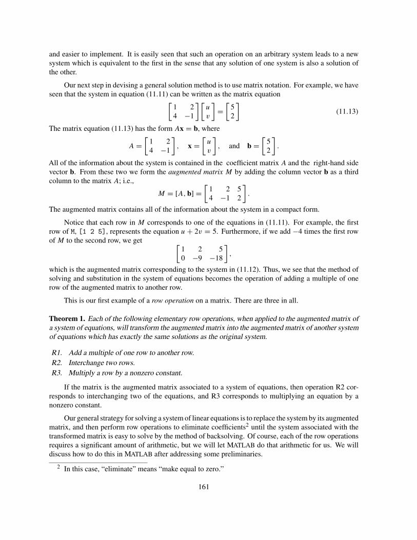
and easier to implement. It is easily seen that such an operation on an arbitrary system leads to a newsystem which is equivalent to the first in the sense that any solution of one system is also a solution ofthe other.

Our next step in devising a general solution method is to use matrix notation. For example, we haveseen that the system in equation (11.11) can be written as the matrix equation

[

1 24 −1

] [

u

v

]

=[

52

]

(11.13)

The matrix equation (11.13) has the form Ax = b, where

A =[

1 24 −1

]

, x =[

u

v

]

, and b =[

52

]

.

All of the information about the system is contained in the coefficient matrix A and the right-hand sidevector b. From these two we form the augmented matrix M by adding the column vector b as a thirdcolumn to the matrix A; i.e.,

M = [A, b] =[

1 2 54 −1 2

]

.

The augmented matrix contains all of the information about the system in a compact form.

Notice that each row in M corresponds to one of the equations in (11.11). For example, the firstrow of M, [1 2 5], represents the equation u + 2v = 5. Furthermore, if we add −4 times the first rowof M to the second row, we get

[

1 2 50 −9 −18

]

,

which is the augmented matrix corresponding to the system in (11.12). Thus, we see that the method ofsolving and substitution in the system of equations becomes the operation of adding a multiple of onerow of the augmented matrix to another row.

This is our first example of a row operation on a matrix. There are three in all.

Theorem 1. Each of the following elementary row operations, when applied to the augmented matrix ofa system of equations, will transform the augmented matrix into the augmented matrix of another systemof equations which has exactly the same solutions as the original system.

R1. Add a multiple of one row to another row.R2. Interchange two rows.R3. Multiply a row by a nonzero constant.

If the matrix is the augmented matrix associated to a system of equations, then operation R2 cor-responds to interchanging two of the equations, and R3 corresponds to multiplying an equation by anonzero constant.

Our general strategy for solving a system of linear equations is to replace the system by its augmentedmatrix, and then perform row operations to eliminate coefficients2 until the system associated with thetransformed matrix is easy to solve by the method of backsolving. Of course, each of the row operationsrequires a significant amount of arithmetic, but we will let MATLAB do that arithmetic for us. We willdiscuss how to do this in MATLAB after addressing some preliminaries.

2 In this case, “eliminate” means “make equal to zero.”

161

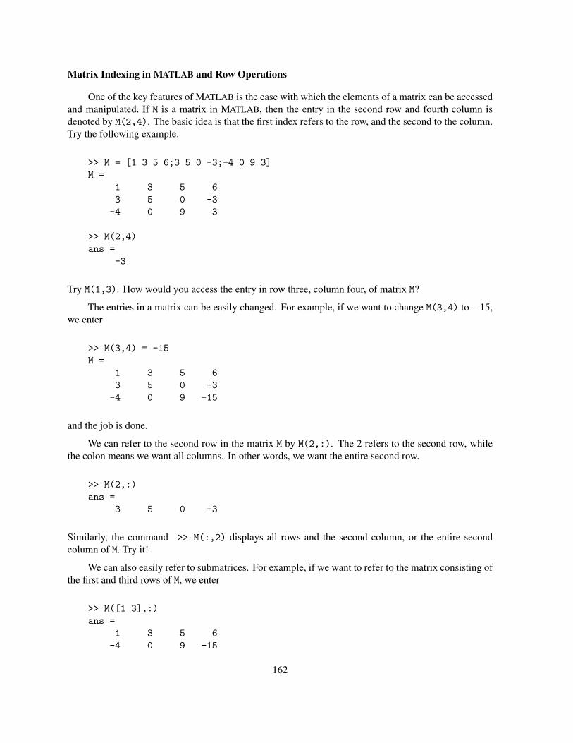
Matrix Indexing in MATLAB and Row Operations

One of the key features of MATLAB is the ease with which the elements of a matrix can be accessedand manipulated. If M is a matrix in MATLAB, then the entry in the second row and fourth column isdenoted by M(2,4). The basic idea is that the first index refers to the row, and the second to the column.Try the following example.

>> M = [1 3 5 6;3 5 0 -3;-4 0 9 3]M =

1 3 5 63 5 0 -3

-4 0 9 3

>> M(2,4)ans =

-3

Try M(1,3). How would you access the entry in row three, column four, of matrix M?

The entries in a matrix can be easily changed. For example, if we want to change M(3,4) to −15,we enter

>> M(3,4) = -15M =

1 3 5 63 5 0 -3

-4 0 9 -15

and the job is done.

We can refer to the second row in the matrix M by M(2,:). The 2 refers to the second row, whilethe colon means we want all columns. In other words, we want the entire second row.

>> M(2,:)ans =

3 5 0 -3

Similarly, the command >> M(:,2) displays all rows and the second column, or the entire secondcolumn of M. Try it!

We can also easily refer to submatrices. For example, if we want to refer to the matrix consisting ofthe first and third rows of M, we enter

>> M([1 3],:)ans =

1 3 5 6-4 0 9 -15

162

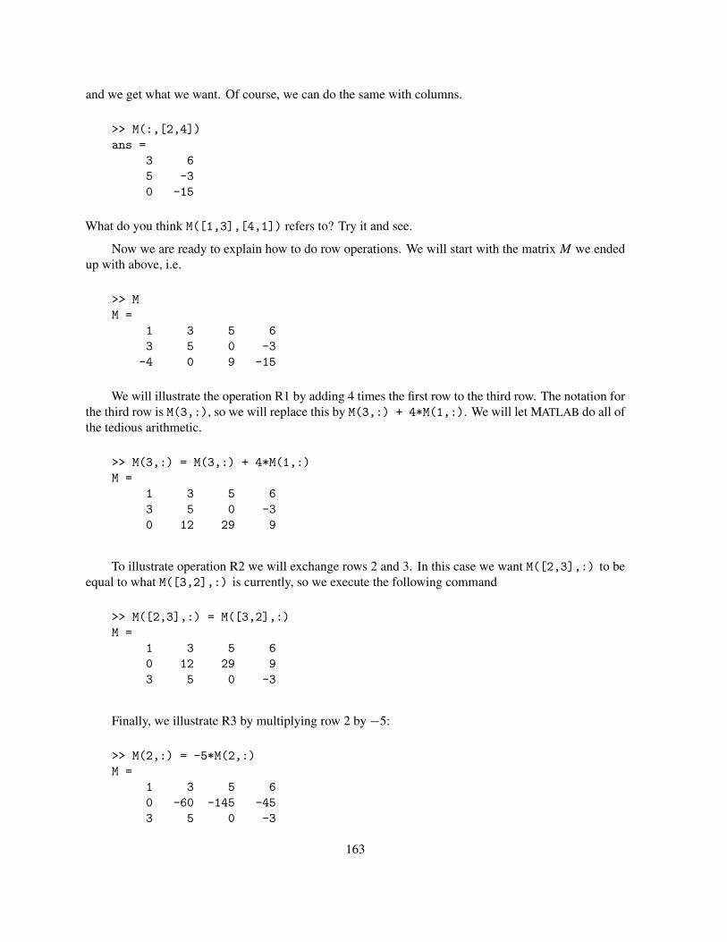
and we get what we want. Of course, we can do the same with columns.

>> M(:,[2,4])ans =

3 65 -30 -15

What do you think M([1,3],[4,1]) refers to? Try it and see.

Now we are ready to explain how to do row operations. We will start with the matrix M we endedup with above, i.e.

>> MM =

1 3 5 63 5 0 -3

-4 0 9 -15

We will illustrate the operation R1 by adding 4 times the first row to the third row. The notation forthe third row is M(3,:), so we will replace this by M(3,:) + 4*M(1,:). We will let MATLAB do all ofthe tedious arithmetic.

>> M(3,:) = M(3,:) + 4*M(1,:)M =

1 3 5 63 5 0 -30 12 29 9

To illustrate operation R2 we will exchange rows 2 and 3. In this case we want M([2,3],:) to beequal to what M([3,2],:) is currently, so we execute the following command

>> M([2,3],:) = M([3,2],:)M =

1 3 5 60 12 29 93 5 0 -3

Finally, we illustrate R3 by multiplying row 2 by −5:

>> M(2,:) = -5*M(2,:)M =

1 3 5 60 -60 -145 -453 5 0 -3

163

We can divide a row by a number just as easily:

>> M(3,:) = M(3,:)/3M =

1.0000 3.0000 5.0000 6.00000 -60.0000 -145.0000 -45.0000

1.0000 1.6667 0 -1.0000

The Rational Format

Frequently problems arise in which the numbers we are using are all rational numbers. The floatingpoint arithmetic that MATLAB uses does not lend itself to maintaining the rational form of numbers.We can sometimes recognize a rational number from the decimal expansions MATLAB gives us, butfrequently, we can’t. For example, in M as it appears above, we know that M(3,2) = 5/3, but we willnot always be so fortunate. MATLAB provides a solution with its rational format. If we enter formatrat at the MATLAB prompt, from that point on MATLAB will display numbers as the ratios of integers.For example,

>> format rat>> pians =

355/113

We know, and MATLAB knows, that π �= 355/113. MATLAB is only displaying an approximationto the answer. But this is no different than what MATLAB always does. The only difference is thatnow MATLAB is using a rational number to approximate π instead of a decimal expansion. It computesand displays the rational number that is closest to the given number within a prescribed tolerance. Theadvantage is that if we know the answer is a rational number, then we know that the rational representationshown us by MATLAB is probably 100% correct.

In the rational format, our current matrix M is

>> MM =

1 3 5 60 -60 -145 -451 5/3 0 -1

Thus we get the precise, rational version of M.

We should warn you about one possibly confusing aspect of the rational format. Sometimes asterisks(∗) appear in the output. This happens when MATLAB is trying to give a rational approximation to avery small number. A very large denominator is required, and the resulting expression will not fit withinthe rational format. When we know that the matrix has entries that are rational numbers with smalldenominators, the small number represented by an asterisk is due to round off error. The entry shouldactually be 0, and it can usually be replaced by 0, but caution is called for in doing so.

164

Elimination and Backsolving

The first part of our strategy for solving systems is to use row operations to put the system into aform which can be easily solved by backsolving. The goal is a matrix in row echelon form. This is amatrix that looks like

⎡

⎢

⎢

⎢

⎢

⎢

⎢

⎢

⎣

P # # # # # # # # #0 P # # # # # # # #0 0 0 0 P # # # # #0 0 0 0 0 P # # # #0 0 0 0 0 0 0 0 P #0 0 0 0 0 0 0 0 0 00 0 0 0 0 0 0 0 0 0

⎤

⎥

⎥

⎥

⎥

⎥

⎥

⎥

⎦

, (11.14)

where the P s stand for nonzero numbers and the #s stand for arbitrary numbers. We will define the pivotof a row in a matrix to be the first nonzero number in that row. Thus the P s in (11.14) are pivots. Thedistinguishing feature of a matrix in row echelon form is that, in any row that has a pivot, the pivot liesstrictly to the right of the pivots in preceding rows.

After working some examples, and some thought, you should be able to convince yourself that anymatrix can be reduced to row echelon form using row operations. In fact, we can go further. The pivotscan all be reduced to 1 by dividing each row of the matrix in (11.14) by its pivot. In addition, all of thenonzero entries above a pivot can be reduced to 0 by adding (or subtracting) a multiple of the pivot row.In this way we can reduce the matrix to the form

⎡

⎢

⎢

⎢

⎢

⎢

⎢

⎢

⎣

1 0 # # 0 0 # # 0 #0 1 # # 0 0 # # 0 #0 0 0 0 1 0 # # 0 #0 0 0 0 0 1 # # 0 #0 0 0 0 0 0 0 0 1 #0 0 0 0 0 0 0 0 0 00 0 0 0 0 0 0 0 0 0

⎤

⎥

⎥

⎥

⎥

⎥

⎥

⎥

⎦

, (11.15)

where the #’s stand for arbitrary numbers. A matrix in the form of (11.15) is said to be in reduced rowechelon form.

Our entire strategy for solving systems of linear equations amounts to taking the augmented matrixof the system and transforming it to row echelon form using elementary row operations. This method iscalled Gaussian elimination. You will learn that a system in row echelon form can be easily solved bybacksolving.

Example 8. Find all solutions to the system

x2 − x3 + 6x4 = 0,

3x1 − 4x2 + 5x3 − x4 = 5,

5x1 − x3 + 4x4 = 4,

(11.16)

for x1, x2, x3, and x4.

165

We first write the system in (11.16) in the matrix form Ax = b, where

A =[ 0 1 −1 6

3 −4 5 −15 0 −1 4

]

, x =⎡

⎢

⎣

x1x2x3x4

⎤

⎥

⎦, and b =

[ 054

]

.

In MATLAB, we first enter A and b and form the augmented matrix:

>> A = [0 1 -1 6;3 -4 5 -1;5 0 -1 4]; b=[0 5 4]'; M = [A,b]M =

0 1 -1 6 03 -4 5 -1 55 0 -1 4 4

Reduction to row echelon form. To start this process we want to get a pivot into the upper left-handcorner. To do so, we use operation R2, and interchange the first and second rows:

>> M([1,2],:) = M([2,1],:)M =

3 -4 5 -1 50 1 -1 6 05 0 -1 4 4

Now that the pivot in the first row is M(1,1) = 3, we want to make all of the entries below it equal to 0in order to move the pivots in the lower rows to the right. Since M(2,1) = 0, we need do nothing to thesecond row. For the third row we subtract 5/3 times the first row to make M(3,1) = 0:

>> M(3,:) = M(3,:) - (5/3)*M(1,:)M =

3 -4 5 -1 50 1 -1 6 00 20/3 -28/3 17/3 -13/3

The pivot in the second row is M(2,2) = 1 and that in the third row is M(3,2) = 20/3. We wantto make M(3,2) = 0 in order to move the pivot in the third row to the right. We can do so by subtracting20/3 times the second row from the third:

>> M(3,:) = M(3,:) - (20/3)*M(2,:)M =

3 -4 5 -1 50 1 -1 6 00 0 -8/3 -103/3 -13/3

The matrix is now in row echelon form, but not in reduced row echelon form. It is the augmentedmatrix for the system

3x1 − 4x2 + 5x3 − x4 = 5

x2 − x3 + 6x4 = 0

−(8/3)x3 − (103/3)x4 = −13/3

(11.17)

166

The system in (11.17) has the same solutions as the system in (11.16), but this one can be easily solvedby backsolving.

Backsolving. We start by solving the last equation in (11.17). This involves only the two variables x3and x4. We can assign an arbitrary value to either one and solve for the other. We need a systematic wayof deciding which variable is assigned the arbitrary value.

We will call a column in a matrix in row echelon form which contains a pivot a pivot column.The corresponding variables are called pivot variables. In our example, columns 1, 2, and 3 are pivotcolumns, and x1, x2, and x3 are the pivot variables. A column which does not contain a pivot is calleda free column. The variables corresponding to free columns are called free variables. Thus column 4 isa free column and x4 is a free variable. Notice that we can assign an arbitrary value to the free variablex4 and still solve (11.17) for the pivot variables. Consequently, we set x4 = t . Then solving the thirdequation in (11.17) for x3 we get

x3 = (13 − 103x4)/8 = (13 − 103t)/8.

Now we can solve the second equation for x2:

x2 = x3 − 6x4 = (13 − 108t)/8 − 6t = (13 − 151t)/8.

Finally, we can solve the first equation for x1:

x1 = (5 + 4x2 − 5x3 + x4) /3

= (5 + 4(13 − 151t)/8 − 5(13 − 103t)/8 + t) /3

= (9 − 27t)/8.

We can sum up our results in vector form. The solutions to (11.17), and therefore to (11.16), are allvectors of the form

x =⎡

⎢

⎣

x1x2x3x4

⎤

⎥

⎦=⎡

⎢

⎣

(9 − 27t)/8(13 − 151t)/8(13 − 103t)/8

t

⎤

⎥

⎦=⎡

⎢

⎣

9/813/813/8

0

⎤

⎥

⎦+ t

⎡

⎢

⎣

−27/8−151/8−103/8

1

⎤

⎥

⎦. (11.18)

This solution is called the general solution, since all possible solutions of system (11.16) can be foundby substituting arbitrary numbers for the parameter t . For example, t = 0 yields the solution x1 = 9/8,x2 = 13/8, x3 = 13/8, and x4 = 0; t = 1 yields the solution x1 = −9/4, x2 = −69/4, x3 = −45/4,and x4 = 1; etc.

Reduction to reduced row echelon form. For the sake of comparison, let’s reduce the augmented matrixM to reduced row echelon form. We will learn an important insight along the way. We need to make thepivots equal to 1, and this is accomplished by dividing each row by its pivot:

>> M(1,:) = M(1,:)/3; M(3,:) = (-3/8)*M(3,:);

167

In addition we have to make the entries above the pivots equal to 0. We can do this by adding multiplesof a row to those above it. The operations to make M(1,2) = 0 and M(1,3) = 0 are

>> M(1,:) = M(1,:) +(4/3)*M(2,:);>> M(1,:) = M(1,:) -(1/3)*M(3,:)M =

1 0 * 27/8 9/80 1 -1 6 00 0 1 103/8 13/8

Here we have a surprise. The asterisk (*) indicates that the entry, M(1,3), is a rational numberwhose rational form is too large to display on the screen. Remember that M(1,3) should be equal to 0.To see what it really is we execute

>> M(1,3)ans =

1/6004799503160662

Thus M(1,3) is a very small number. MATLAB is making small roundoff errors all the time, and this isthe result. We have been a little careless. When we do row operations, we will get better precision if werefer to the matrix elements by name instead of using the number that MATLAB is using to display themon the screen. For example, if we execute

>> M(1,:) = M(1,:) -M(1,3)*M(3,:)M =

1 0 0 27/8 9/80 1 -1 6 00 0 1 103/8 13/8

we are back on track. Notice that we referred directly to M(1,3) in this command. This is the preferredmethod for doing row operations. We will use this procedure in the future, and we recommend that youdo too. For example, the command to make M(2,3) equal to 0 is

>> M(2,:) = M(2,:) - M(2,3)*M(3,:)M =

1 0 0 27/8 9/80 1 0 151/8 13/80 0 1 103/8 13/8

which gives us the reduced row echelon form for the augmented matrix.

This matrix is the augmented matrix for the system

x1 + (27/8)x4 = 9/8,

x2 + (151/8)x4 = 13/8,

x3 + (103/8)x4 = 13/8.

(11.19)

168

Of course, the system in (11.19) has the same solutions as the systems in (11.16) and (11.17). Solving tofind the solutions given in (11.18) is extremely easy. However, we had to do five additional row operationsto get to reduced row echelon form and the easier system in (11.19). This raises a question. Starting atthe row echelon form we have two ways to proceed. We can either solve the system given by the rowechelon form, or we can perform the additional row operations to get to reduced row echelon form andthe easier system. Both give the correct answer, but which is the easiest method? This is a hard questionto answer, but most people find it preferable to stop at row echelon form, and not do the additional workof reducing the augmented matrix to reduced row echelon form. Try it both ways, and choose the methodwhich is easiest for you.

The method we used on Example 8 works for any system. Let’s list the steps in the process.

Summary: Method of solution for a system of linear equations.

1. Write the system in the matrix form Ax = b and form the augmented matrix M = [A, b].2. Use row operations to reduce M to row echelon form.3. Write down the simplified system.4. Solve the simplified system by backsolving:

• Assign arbitrary values to the free variables.• Backsolve for the pivot variables.

The MATLAB command rref. After completing Example 8, you must be wondering why the computerand MATLAB can’t do step 2 in the solution process, the reduction of a matrix to row echelon form, oreven to reduced row echelon form, with a single command. In fact it can. If we start with the originalaugmented matrix

>> M = [A,b];

then we can proceed directly to the reduced row echelon form by using the MATLAB command rref.

>> MR = rref(M)MR =

1 0 0 27/8 9/80 1 0 151/8 13/80 0 1 103/8 13/8

This eliminates all of the intermediate steps, and we can proceed to the third step and write down theequivalent system of equations as we did in (11.19).

Example 9. Find all solutions to the system

2x2 + 2x3 + 3x4 = −4,

−2x1 + 4x2 + 2x3 − x4 = −6,

3x1 − 4x2 − x3 + 2x4 = 8.

169

The augmented matrix is

>> M = [0 2 2 3 -4; -2 4 2 -1 -6; 3 -4 -1 2 8]M =

0 2 2 3 -4-2 4 2 -1 -63 -4 -1 2 8

Place the augmented matrix in reduced row echelon form:

>> rref(M)ans =

1 0 1 0 16/50 1 1 0 -1/50 0 0 1 -6/5

Notice that columns 1, 2, and 4 are pivot columns, so x1, x2, and x4 are pivot variables and x3 is a freevariable. The equivalent system is

x1 + x3 = 16/5,

x2 + x3 = −1/5,

x4 = −6/5.

Solve each of the above equations for a pivot variable, in terms of the free variable x3.

x1 = 16/5 − x3

x2 = −1/5 − x3

x4 = −6/5

Set x3 = t , where t is an arbitrary number, and we see that the solutions of the system are all vectors ofthe form

x =⎡

⎢

⎣

x1x2x3x4

⎤

⎥

⎦=⎡

⎢

⎣

16/5 − t

−1/5 − t

t

−6/5

⎤

⎥

⎦=⎡

⎢

⎣

16/5−1/5

0−6/5

⎤

⎥

⎦+ t

⎡

⎢

⎣

−1−1

10

⎤

⎥

⎦,

where t is arbitrary.

Determined Systems of Equations

A system is determined if it has the same number of equations and unknowns. It is underdeterminedif it has fewer equations than unknowns, and overdetermined if it has more equations than unknowns.Some of the systems we have been solving up to now have been underdetermined. In this section weexamine determined systems.

There are three possibilities for the set of all solutions to a system of linear equations:

• there are no solutions,• there are infinitely many solutions,• there is a unique solution.

170

The next three examples of determined systems illustrate these possibilities.

Example 10. Find all solutions to the system

4x1 − 4x2 − 8x3 = 27,

2x2 + 2x3 = −6,

x1 − 2x2 − 3x3 = 10.

(11.20)

The system in (11.20) is determined, since it has three unknowns (x1, x2, and x3) and three equations.Set up the augmented matrix

>> M = [4 -4 -8 27;0 2 2 -6;1 -2 -3 10]M =

4 -4 -8 270 2 2 -61 -2 -3 10

and find its reduced row echelon form.

>> rref(M)ans =

1 0 -1 00 1 1 00 0 0 1

The last row of the reduced row echelon form represents the equation 0x1 +0x2 +0x3 = 1, which clearlyhas no solutions. If there is no solution which satisfies this last equation, then there certainly cannot be asolution which satisfies all three equations represented by the matrix. Consequently, the system (11.20)has no solutions. A system that has solutions is called a consistent system. Since this system has nosolutions it is inconsistent.

Example 11. Find all solutions to the system

4x1 − 4x2 − 8x3 = 4,

2x2 + 2x3 = 2,

x1 − 2x2 − 3x3 = 0.

(11.21)

The system in (11.21) is determined, since it has three unknowns (x1, x2, and x3) and three equations.Set up the augmented matrix

>> M = [4 -4 -8 4;0 2 2 2;1 -2 -3 0]M =

4 -4 -8 40 2 2 21 -2 -3 0

171

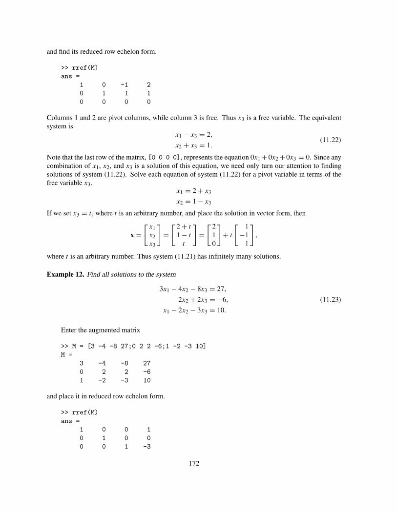
and find its reduced row echelon form.

>> rref(M)ans =

1 0 -1 20 1 1 10 0 0 0

Columns 1 and 2 are pivot columns, while column 3 is free. Thus x3 is a free variable. The equivalentsystem is

x1 − x3 = 2,

x2 + x3 = 1.(11.22)

Note that the last row of the matrix, [0 0 0 0], represents the equation 0x1 + 0x2 + 0x3 = 0. Since anycombination of x1, x2, and x3 is a solution of this equation, we need only turn our attention to findingsolutions of system (11.22). Solve each equation of system (11.22) for a pivot variable in terms of thefree variable x3.

x1 = 2 + x3

x2 = 1 − x3

If we set x3 = t , where t is an arbitrary number, and place the solution in vector form, then

x =[

x1x2x3

]

=[ 2 + t

1 − t

t

]

=[ 2

10

]

+ t

[ 1−1

1

]

,

where t is an arbitrary number. Thus system (11.21) has infinitely many solutions.

Example 12. Find all solutions to the system

3x1 − 4x2 − 8x3 = 27,

2x2 + 2x3 = −6,

x1 − 2x2 − 3x3 = 10.

(11.23)

Enter the augmented matrix

>> M = [3 -4 -8 27;0 2 2 -6;1 -2 -3 10]M =

3 -4 -8 270 2 2 -61 -2 -3 10

and place it in reduced row echelon form.

>> rref(M)ans =

1 0 0 10 1 0 00 0 1 -3

172

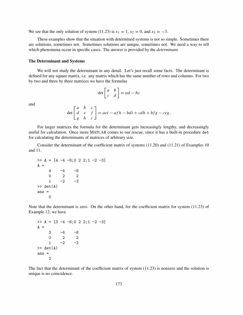
We see that the only solution of system (11.23) is x1 = 1, x2 = 0, and x3 = −3.

These examples show that the situation with determined systems is not so simple. Sometimes thereare solutions, sometimes not. Sometimes solutions are unique, sometimes not. We need a way to tellwhich phenomena occur in specific cases. The answer is provided by the determinant.

The Determinant and Systems

We will not study the determinant in any detail. Let’s just recall some facts. The determinant isdefined for any square matrix, i.e. any matrix which has the same number of rows and columns. For twoby two and three by three matrices we have the formulas

det

[

a b

c d

]

= ad − bc

and

det

[

a b c

d e f

g h i

]

= aei − af h − bdi + cdh + bfg − ceg.

For larger matrices the formula for the determinant gets increasingly lengthy, and decreasinglyuseful for calculation. Once more MATLAB comes to our rescue, since it has a built-in procedure detfor calculating the determinants of matrices of arbitrary size.

Consider the determinant of the coefficient matrix of systems (11.20) and (11.21) of Examples 10and 11.

>> A = [4 -4 -8;0 2 2;1 -2 -3]A =

4 -4 -80 2 21 -2 -3

>> det(A)ans =

0

Note that the determinant is zero. On the other hand, for the coefficient matrix for system (11.23) ofExample 12, we have

>> A = [3 -4 -8;0 2 2;1 -2 -3]A =

3 -4 -80 2 21 -2 -3

>> det(A)ans =

2

The fact that the determinant of the coefficient matrix of system (11.23) is nonzero and the solution isunique is no coincidence.

173

Theorem 2. Let A be an n × n matrix.

a) If det A �= 0, then for every column n-vector b there is a unique vector x such that Ax = b. Inparticular, the only solution to the homogeneous equation Ax = 0 is the zero vector, x = 0.

b) If det(A) = 0, then there are vectors b for which there are no vectors x with Ax = b. If there isa solution to the equation Ax = b, then there are infinitely many. In particular, the homogeneousequation Ax = 0 has nonzero solutions.

If det A = 0, we will say that the matrix A is singular. As we saw in Examples 10 and 11, if thecoefficient matrix is singular, then two possibilities exist. Either the system Ax = b has no solutions, orit has infinitely many solutions.

On the other hand, if det A �= 0, we will say that A is nonsingular. If the matrix A is nonsingular,then the system Ax = b has a unique solution for every choice of b. MATLAB has a convenient way tofind this solution. It is only necessary to enter x = A\b. Hence, system (11.23) can be solved as follows:

>> A = [3 -4 -8;0 2 2;1 -2 -3];b=[27;-6;10];>> x = A\bx =

11/1125899906842624-3

The very large denominator in the second term indicates that MATLAB is approximating 0. (Look at thisanswer in format long.) Thus, this solution agrees with the one found in Example 12. On the otherhand, if we try the same technique on system (11.20) of Example 10, we get

>> A = [4 -4 -8;0 2 2;1 -2 -3];b=[27;-6;10];>> x = A\b

Warning: Matrix is singular to working precision.x =

1/01/01/0

we see that MATLAB recognizes the fact that A is a singular matrix.

The backslash command A\b is deceptively simple. It looks as if we are dividing the equationAx = b on the left by the matrix A to produce the solution x = A\b. In a way this is true, but in order toimplement that division, MATLAB has to go through a series of computations involving row operationswhich is very similar to those discussed in this chapter.

If the matrix A is nonsingular, then it has an inverse. This is another matrix B such that AB =BA = I . Here I is the identity matrix, which has all ones along the diagonal, and zeros off the diagonal.In general it is time-consuming to calculate the inverse of a matrix, but again MATLAB can do this forus. We enter B = inv(A). For example, if A is the coefficient matrix of system (11.23), then

174

>> A = [3 -4 -8;0 2 2;1 -2 -3]A =

3 -4 -80 2 21 -2 -3

>> B = inv(A)B =

-1 2 41 -1/2 -3

-1 1 3

You can verify that BA = AB = I , with B*A and A*B. Try it! By the way, in MATLAB the commandeye(n) is used to designate the n × n identity matrix. Try eye(3).

The Nullspace of a Matrix

The nullspace of a matrix A is the set of all vectors x such that Ax = 0. Because x = 0 is always asolution of Ax = 0, the zero vector is always an element of the nullspace of matrix A. However, if A isnonsingular, then Theorem 2 guarantees that this solution is unique, and the nullspace of A consists ofonly the zero vector 0. On the other hand, if matrix A is singular, then the nullspace will contain lots ofnon-zero vectors.

Example 13. Find the nullspace of matrix

A =⎡

⎢

⎣

12 −8 −4 303 −2 −1 6

18 −12 −6 426 −4 −2 15

⎤

⎥

⎦.

The nullspace of A consists of all solutions of Ax = 0, or⎡

⎢

⎣

12 −8 −4 303 −2 −1 6

18 −12 −6 426 −4 −2 15

⎤

⎥

⎦

⎡

⎢

⎣

x1x2x3x4

⎤

⎥

⎦=⎡

⎢

⎣

0000

⎤

⎥

⎦. (11.24)

Set up the augmented matrix with the commands

>> A = [12 -8 -4 30;3 -2 -1 6;18 -12 -6 42;6 -4 -2 15];>> b = zeros(4,1);>> M = [A,b];

and find its reduced row echelon form,

>> rref(M)ans =

1 -2/3 -1/3 0 00 0 0 1 00 0 0 0 00 0 0 0 0

175

Note that the pivot columns are one and four, making x1 and x4 pivot variables, leaving x2 and x3 as freevariables. The equivalent system is

x1 − (2/3)x2 − (1/3)x3 = 0,

x4 = 0.(11.25)

Solve each equation of system (11.25) for a pivot variable, in terms of the free variables x2 and x3.

x1 = (2/3)x2 + (1/3)x3

x4 = 0

Set x2 = s and x3 = t , where s and t are arbitrary numbers, then write the solution in vector form.

x =⎡

⎢

⎣

x1x2x3x4

⎤

⎥

⎦=⎡

⎢

⎣

(2/3)s + (1/3)t

s

t

0

⎤

⎥

⎦=⎡

⎢

⎣

(2/3)s

s

00

⎤

⎥

⎦+⎡

⎢

⎣

(1/3)t

0t

0

⎤

⎥

⎦= s

⎡

⎢

⎣

2/3100

⎤

⎥

⎦+ t

⎡

⎢

⎣

1/3010

⎤

⎥

⎦

Thus, every element in the nullspace of matrix A can be written as a linear combination of the vectorsv1 = [2/3, 1, 0, 0]T and v2 = [1/3, 0, 1, 0]T . The nullspace contains infinitely many vectors, but if weknow v1 and v2 we know them all.

The results in this example are typical of what happens in general. The nullspace of a matrix willconsist of all linear combinations of a small number of special vectors. If these vectors are linearlyindependent (see the next section), they are called a basis of the nullspace, and the nullspace is said tobe spanned by the basis vectors. If we know a basis for a nullspace, then we know all of the vectors inthe nullspace. For this reason we will almost always describe a nullspace by giving a basis.

Linear Dependence and Independence

A finite set of vectors is said to be linearly independent if the only linear combination which is equalto the zero vector is the one where all of the coefficients are equal to zero; i.e., the vectors v1, v2, · · · , vp

are linearly independent if c1v1 + c2v2 + · · · + cpvp = 0 implies that c1 = c2 = · · · = cp = 0. A set ofvectors which is not linearly independent is said to be linearly dependent.

Example 14. Show that the vectors

v1 =[ 1

11

]

, v2 =[ 0

−12

]

, and v3 =[ 2

−18

]

are linearly dependent.

We need to find a non-trivial solution of

c1

[ 111

]

+ c2

[ 0−1

2

]

+ c3

[ 2−1

8

]

=[ 0

00

]

. (11.26)

176

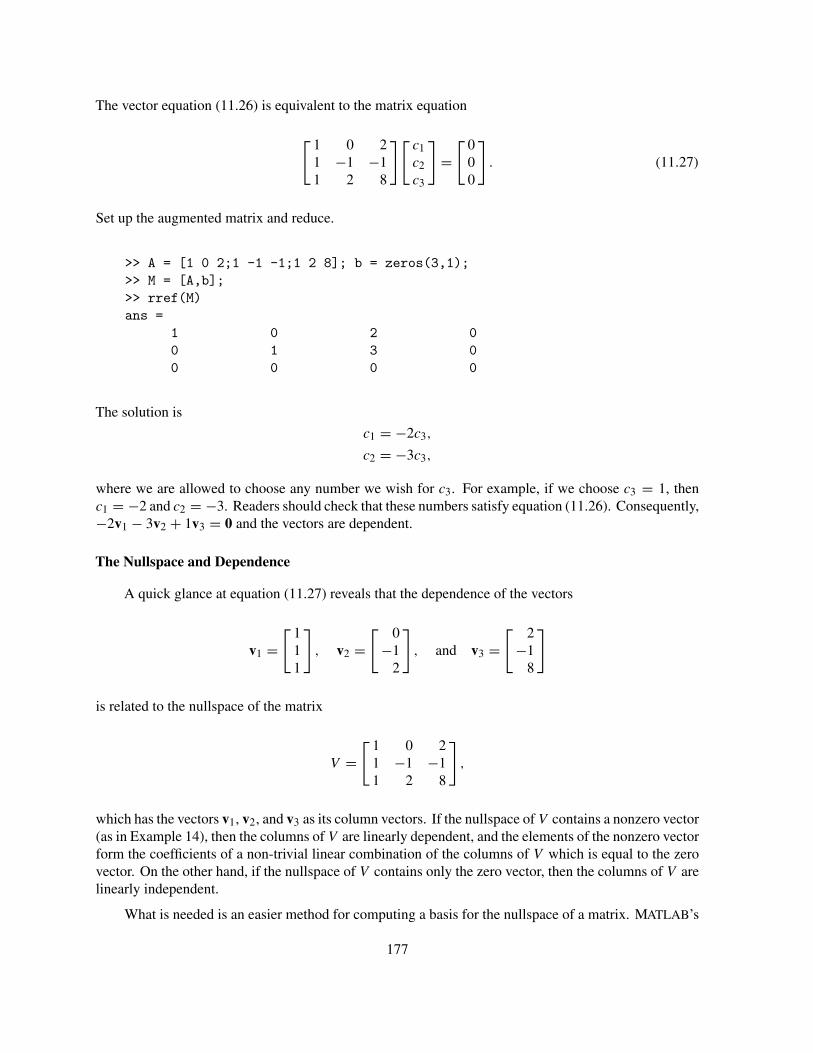
The vector equation (11.26) is equivalent to the matrix equation

[ 1 0 21 −1 −11 2 8

][

c1c2c3

]

=[ 0

00

]

. (11.27)

Set up the augmented matrix and reduce.

>> A = [1 0 2;1 -1 -1;1 2 8]; b = zeros(3,1);>> M = [A,b];>> rref(M)ans =

1 0 2 00 1 3 00 0 0 0

The solution is

c1 = −2c3,

c2 = −3c3,

where we are allowed to choose any number we wish for c3. For example, if we choose c3 = 1, thenc1 = −2 and c2 = −3. Readers should check that these numbers satisfy equation (11.26). Consequently,−2v1 − 3v2 + 1v3 = 0 and the vectors are dependent.

The Nullspace and Dependence

A quick glance at equation (11.27) reveals that the dependence of the vectors

v1 =[ 1

11

]

, v2 =[ 0

−12

]

, and v3 =[ 2

−18

]

is related to the nullspace of the matrix

V =[ 1 0 2

1 −1 −11 2 8

]

,

which has the vectors v1, v2, and v3 as its column vectors. If the nullspace of V contains a nonzero vector(as in Example 14), then the columns of V are linearly dependent, and the elements of the nonzero vectorform the coefficients of a non-trivial linear combination of the columns of V which is equal to the zerovector. On the other hand, if the nullspace of V contains only the zero vector, then the columns of V arelinearly independent.

What is needed is an easier method for computing a basis for the nullspace of a matrix. MATLAB’s

177

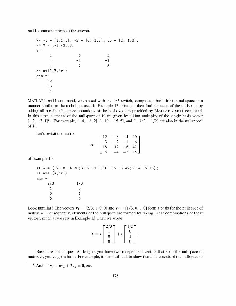
null command provides the answer.

>> v1 = [1;1;1]; v2 = [0;-1;2]; v3 = [2;-1;8];>> V = [v1,v2,v3]V =

1 0 21 -1 -11 2 8

>> null(V,'r')ans =

-2-31

MATLAB’s null command, when used with the 'r' switch, computes a basis for the nullspace in amanner similar to the technique used in Example 13. You can then find elements of the nullspace bytaking all possible linear combinations of the basis vectors provided by MATLAB’s null command.In this case, elements of the nullspace of V are given by taking multiples of the single basis vector[−2, −3, 1]T . For example, [−4, −6, 2], [−10, −15, 5], and [1, 3/2, −1/2] are also in the nullspace3

of V .

Let’s revisit the matrix

A =⎡

⎢

⎣

12 −8 −4 303 −2 −1 6

18 −12 −6 426 −4 −2 15

⎤

⎥

⎦

of Example 13.

>> A = [12 -8 -4 30;3 -2 -1 6;18 -12 -6 42;6 -4 -2 15];>> null(A,'r')ans =

2/3 1/31 00 10 0

Look familiar? The vectors v1 = [2/3, 1, 0, 0] and v2 = [1/3, 0, 1, 0] form a basis for the nullspace ofmatrix A. Consequently, elements of the nullspace are formed by taking linear combinations of thesevectors, much as we saw in Example 13 when we wrote

x = s

⎡

⎢

⎣

2/3100

⎤

⎥

⎦+ t

⎡

⎢

⎣

1/3010

⎤

⎥

⎦.

Bases are not unique. As long as you have two independent vectors that span the nullspace ofmatrix A, you’ve got a basis. For example, it is not difficult to show that all elements of the nullspace of

3 And −4v1 − 6v2 + 2v2 = 0, etc.

178

matrix A can also be written as linear combinations of the independent vectors w1 = [2, 3, 0, 0]T andw2 = [1, 0, 3, 0]T . Also, consider the output from MATLAB’s null command, this time without the 'r'switch.

>> format, null(A)ans =

-0.5976 0.0033-0.7196 -0.4432-0.3536 0.8964-0.0000 -0.0000

The command format returns the command window to the standard output format. The output of thisnull command is normalized so that the sum of the squares of the entries of each column vector equalsone, and the dot product of different column vectors equals zero. This basis is called an orthonormalbasis and is very useful in certain situations.

Although bases are not unique, it is true that every basis for the nullspace must contain the samenumber of vectors. This number is called the dimension of the nullspace. Thus, the nullspace of matrixA has dimension equal to 2; and, should you find another basis for the nullspace of the matrix A, it willalso contain two vectors.

Example 15. Discuss the dependence of the vectors

v1 =[ 1

−14

]

, v2 =[−2

45

]

, and v1 =[−2

1043

]

.

>> v1 = [1;-1;4]; v2 = [-2;4;5]; v3 = [-2;10;43];>> V = [v1,v2,v3]V =

1 -2 -2-1 4 104 5 43

>> null(V,'r')ans =

Empty matrix: 3-by-0

This response means that there are no nonzero vectors in the nullspace, so we conclude that the vectorsare linearly independent.

Exercises

In Exercises 1 – 4, find the general solution to each of the indicated system of linear equations using the method ofrow operations. You may use MATLAB to perform the operations, but in your submission show all of the operationsthat you perform. In other words, do not use rref. Use the diary command (as explained in Chapter 1) to recordyour work.

179

1. −5x + 14y = −47−7x + 16y = −55

2. 2x1 − 5x2 + 3x3 = 84x1 + 3x2 − 7x3 = −3

3. −6x − 8y + 8z = −309x + 11y − 8z = 339x + 9y − 6z = 27

4. −19x1 − 128x2 + 81x3 + 38x4 = 08x1 + 61x2 − 27x3 − 16x4 = 02x1 + 4x2 + 12x3 − 4x4 = 0

−8x1 − 16x2 + 12x3 + 16x4 = 0

In Exercises 5 – 10, find the general solution to the indicated system of linear equations. You may use rref, andthe backslash operation (A\b) if it applies.

5. −x − 9y + 6z = 152x + 9y + z = −16

6. 8x − 10y − 228z = −1122x − y − 4z = −164x − 5y − 14z = −56

7. −19x1 − 128x2 + 81x3 + 38x4 = 38x1 + 61x2 − 27x3 − 16x4 = 52x1 + 4x2 + 12x3 − 4x4 = −21

−8x1 − 16x2 + 12x3 + 16x4 = −4

8. 2x + 2z = 6x + z = 3

−7x + 12y + 5z = 27

9. 23 x1 − 2

3 x3 + 13 x4 = 1

3112 x1 − 3x2 − 20

3 x3 + 13 x4 = − 80

3

−3x1 + 3x2 + 6x3 = 27

− 163 x1 + 6x2 + 34

3 x3 + 13 x4 = 163

3

10. −23x1 + 26x2 − 42x3 − 32x4 − 90x5 = −6

−2x1 + x2 − 3x4 − 4x5 = −2

−17x1 + 19x2 − 28x3 − 22x4 − 63x5 = −3

−14x1 + 14x2 − 24x3 − 16x4 − 52x5 = −2

18x1 − 20x2 + 32x3 + 23x4 + 69x5 = 3

In Exercises 11 – 16, find a basis for the nullspace of the indicated matrix. What is the dimension of the nullspace?

11.

[

2 2−1 −1

]

12.

[ 0 4 −21 −2 13 −10 5

]

13.

[ 2 −4 −90 0 −20 0 1

]

14.

⎡

⎢

⎣

12 −5 −14 −918 −7 −22 −1212 −6 −12 −9

−16 8 16 11

⎤

⎥

⎦

15.

⎡

⎢

⎣

−3 2 5 26 −2 −8 −2

−4 2 6 2−4 2 6 2

⎤

⎥

⎦16.

⎡

⎢

⎢

⎢

⎣

6 −4 2 −12 −86 −4 2 −12 −8

29 −14 11 −54 −3613 −6 5 −24 −16

−10 4 −4 18 12

⎤

⎥

⎥

⎥

⎦

In Exercises 17 – 23, determine if the set of vectors is linearly dependent or independent. If they are dependent, finda nonzero linear combination which is equal to the zero vector.

17.

[

12

]

and

[−3−6

]

18.

[

12

]

and

[−3−5

]

19.

[ 120

]

and

[−3−6

1

]

20.

[ 111

]

,

[ 1−1

1

]

, and

[ 505

]

21.

[ 111

]

,

[ 1−1

1

]

, and

[ 515

]

22.

⎡

⎢

⎣

1010

⎤

⎥

⎦,

⎡

⎢

⎣

0111

⎤

⎥

⎦, and

⎡

⎢

⎣

5−6−1−6

⎤

⎥

⎦

23.

⎡

⎢

⎣

1010

⎤

⎥

⎦,

⎡

⎢

⎣

0111

⎤

⎥

⎦, and

⎡

⎢

⎣

5−6

0−6

⎤

⎥

⎦

180

12. Homogeneous Linear Systems of ODEs

A system of first order differential equations is linear, homogeneous, and has constant coefficientsif it has the specific form

x1′ = a11x1 + a12x2 + · · · + a1nxn,

x2′ = a21x1 + a22x2 + · · · + a2nxn,

...

xn′ = an1x1 + an2x2 + · · · + annxn,

(12.1)

where each aij is a constant. System (12.1) can be written in matrix form

x′ =

⎡

⎢

⎢

⎣

x1x2...

xn

⎤

⎥

⎥

⎦

′

=

⎡

⎢

⎢

⎣

a11 a12 · · · a1n

a21 a22 · · · a2n...

.... . .

...

an1 an2 · · · ann

⎤

⎥

⎥

⎦

⎡

⎢

⎢

⎣

x1x2...

xn

⎤

⎥

⎥

⎦

= Ax. (12.2)

The equation x′ = Ax in (12.2) is strikingly similar to the simple first order differential equation

x′ = λx. (12.3)

It is easy to check thatx = Ceλt

is a solution to equation (12.3), where C is an arbitrary constant. Consequently, it seems natural that weshould first try to find a solution of equation x′ = Ax having the form

x = eλtv, (12.4)

where v is a column n-vector of constants. The constant function x = 0 is a solution of equation (12.2),but not a very interesting one. Let’s agree that we want to find non-zero solutions of equation (12.2).That is, we wish to find a solution of the form x = eλtv, where v is a non-zero vector of constants (someof the entries in v may be zero, but not all). If we substitute equation (12.4) into the left- and right-handsides of the equation x′ = Ax, we get

x′ = (eλtv)′ = λeλtv and

Ax = A(

eλtv) = eλtAv.

For these to be equal we must have λeλtv = eλtAv. If we divide both sides of this equation by eλt , whichis non-zero, we arrive at

Av = λv. (12.5)

The problem of finding a solution of equation (12.2) is now reduced to finding a number λ and a non-zerovector of constants v that satisfy the equation Av = λv.

181

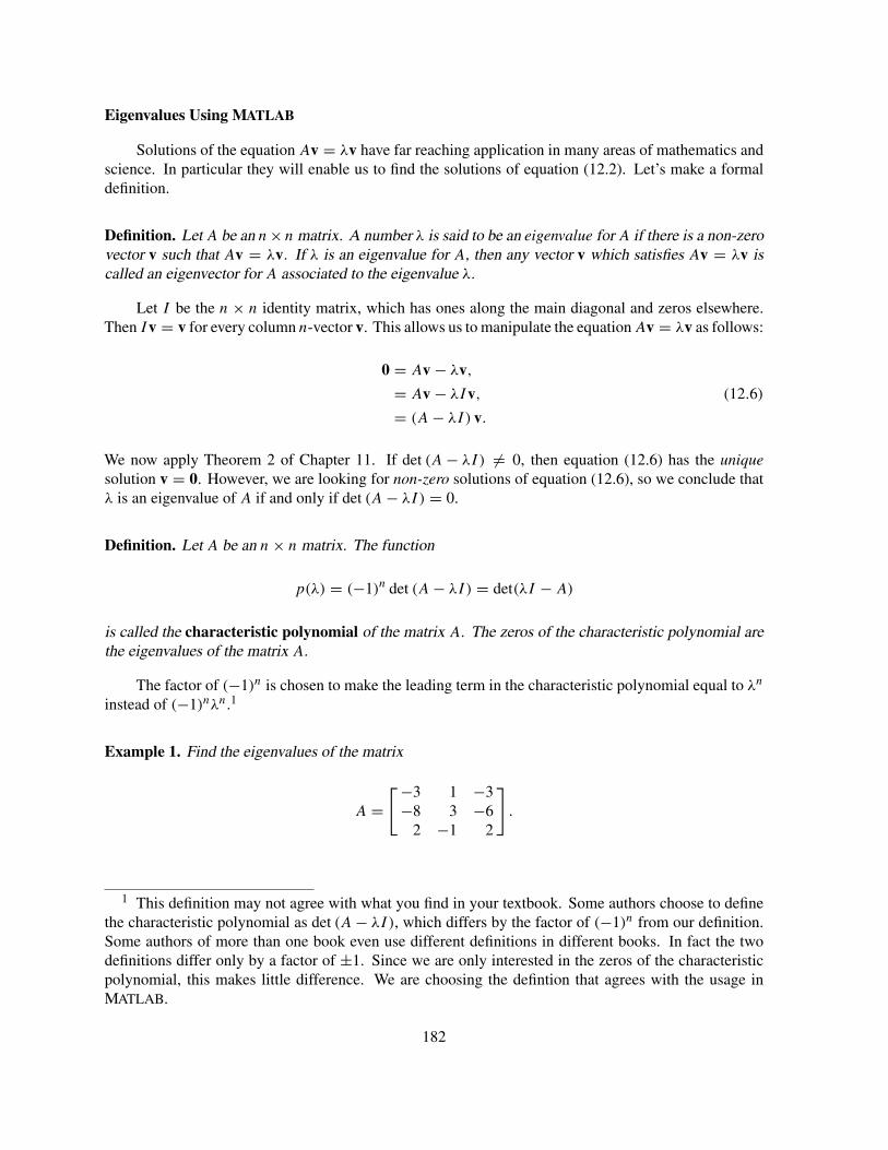
Eigenvalues Using MATLAB

Solutions of the equation Av = λv have far reaching application in many areas of mathematics andscience. In particular they will enable us to find the solutions of equation (12.2). Let’s make a formaldefinition.

Definition. Let A be an n × n matrix. A number λ is said to be an eigenvalue for A if there is a non-zerovector v such that Av = λv. If λ is an eigenvalue for A, then any vector v which satisfies Av = λv iscalled an eigenvector for A associated to the eigenvalue λ.

Let I be the n × n identity matrix, which has ones along the main diagonal and zeros elsewhere.Then Iv = v for every column n-vector v. This allows us to manipulate the equation Av = λv as follows:

0 = Av − λv,

= Av − λIv,

= (A − λI) v.

(12.6)

We now apply Theorem 2 of Chapter 11. If det (A − λI) �= 0, then equation (12.6) has the uniquesolution v = 0. However, we are looking for non-zero solutions of equation (12.6), so we conclude thatλ is an eigenvalue of A if and only if det (A − λI) = 0.

Definition. Let A be an n × n matrix. The function

p(λ) = (−1)n det (A − λI) = det(λI − A)

is called the characteristic polynomial of the matrix A. The zeros of the characteristic polynomial arethe eigenvalues of the matrix A.

The factor of (−1)n is chosen to make the leading term in the characteristic polynomial equal to λn

instead of (−1)nλn.1

Example 1. Find the eigenvalues of the matrix

A =[−3 1 −3

−8 3 −62 −1 2

]

.

1 This definition may not agree with what you find in your textbook. Some authors choose to definethe characteristic polynomial as det (A − λI), which differs by the factor of (−1)n from our definition.Some authors of more than one book even use different definitions in different books. In fact the twodefinitions differ only by a factor of ±1. Since we are only interested in the zeros of the characteristicpolynomial, this makes little difference. We are choosing the defintion that agrees with the usage inMATLAB.

182

We start by calculating the characteristic polynomial. Notice that n = 3 in this case, so

p(λ) = (−1)3 det (A − λI) ,

= − det

([−3 1 −3−8 3 −6

2 −1 2

]

− λ

[ 1 0 00 1 00 0 1

])

,

= − det

[−3 − λ 1 −3−8 3 − λ −62 −1 2 − λ

]

,

= λ3 − 2λ2 − λ + 2.

Of course, this last step requires that we are pretty good at calculating the determinant of a rathercomplicated matrix. MATLAB can help you with the computation.

>> A = [-3 1 -3;-8 3 -6;2 -1 2];>> p = poly(A)p =

1.0000 -2.0000 -1.0000 2.0000

Note that the vector p = [1 -2 -1 2] contains the coefficients of the characteristic polynomial p(λ) =λ3 − 2λ2 −λ+ 2. To find the eigenvalues we must find the zeros of the characteristic polynomial. If youare good at factoring you will discover that

p(λ) = λ3 − 2λ2 − λ + 2 = (λ − 1)(λ + 1)(λ − 2).

Thus, the eigenvalues of A are λ = 1, −1, and 2. MATLAB can help you find the roots. If the vectorp contains the coefficients of the characteristic polynomial, then we can use roots(p) to compute thezeros of p.

>> roots(p)ans =

-1.00002.00001.0000

Symbolic Toolbox Users. If you change your matrix into a symbolic object, Maple can be called uponto perform the evaluations. For example,

>> ps = poly(sym(A))ps =x^3-2*x^2-x+2

computes the characteristic polynomial as a mathematical expression. You can then factor the polynomialwith the command

>> factor(ps)ans =(x-1)*(x-2)*(x+1)

183

It is clear that the zeros are 1, 2, and −1, but you can also use the Symbolic Toolbox’s solve command.

>> solve(ps)ans =[ -1][ 1][ 2]

Eigenvectors Using MATLAB

Having found the eigenvalues, we must now find the associated eigenvectors. Let’s look again atequation (12.6), which we now write as

(A − λI) v = 0. (12.7)

This is the equation which must be solved by an eigenvalue λ and an associated eigenvector v. Thismeans that the eigenvector v is an element of the nullspace of the matrix A − λI .

Example 2. Find the eigenvectors of the matrix

A =[−3 1 −3

−8 3 −62 −1 2

]

.

The eigenvalues of the matrix A were found in Example 1 to be λ = 1, −1, and 2. Select one ofthe eigenvalues, say λ1 = 1. The eigenvectors associated with λ1 = 1 are the vectors in the nullspace ofA − λ1I = A − 1I . These can be found using the methods of Chapter 11. We could use row operations,but we shall use the command null. (Notice that the 3 × 3 identity matrix I is generated with theMATLAB command eye(3).)

>> v1 = null(A - 1*eye(3),'r')v1 =

-1-11

The vectors in the nullspace of A−1I are the multiples of v1, and they are all eigenvectors. Any nonzeromultiple of v1 will serve our purpose, so let’s choose v1 itself.

In a similar manner, the MATLAB commands

>> v2 = null(A - (-1)*eye(3),'r')v2 =

0.50001.0000

0

184

>> v3 = null(A - 2*eye(3),'r')v3 =

-1-21

provide eigenvectors v2 = [1/2, 1, 0]T and v3 = [−1, −2, 1]T associated with the eigenvalues λ2 = −1and λ3 = 2, respectively. Any nonzero multiples of these vectors would also be suitable2. For example,we might want our vectors to contain only integer entries, in which case we could choose v2 = [1, 2, 0]T

for the eigenvalue λ2 = −1.

Symbolic Toolbox Users. The null command works equally well with symbolic objects, but the 'r'switch is not needed.

>> v2 = null(sym(A) - (-1)*eye(3))v2 =[ 1][ 2][ 0]

Finally, you can easily check your solution, symbolically (with the Symbolic Toolbox) or numerically(with MATLAB). For example, use the Symbolic Toolbox to show that Av2 = −1v2.

>> A*v2, -1*v2ans =[ -1][ -2][ 0]ans =[ -1][ -2][ 0]

Since Av2 = −1v2, v2 is an eigenvector with associated eigenvalue λ2 = −1.

MATLAB’s eig Command

Finding eigenvalues and eigenvectors in the manner described requires three steps. First, findthe characteristic polynomial; second, find the eigenvalues, which are the roots of the characteristicpolynomial; and third, for each eigenvalue λ, find the associated eigenvectors by finding the nullspace ofA−λI . This three step process can be replaced with a one step process using MATLAB’s eig command.

Example 3. Use MATLAB’s eig command to find the eigenvalues and eigenvectors of

A =[−3 1 −3

−8 3 −62 −1 2

]

.

2 If v is an eigenvector of matrix A associated with the eigenvalue λ, then A(cv) = c(Av) = c(λv) =λ(cv), making cv an eigenvector for any constant number c.

185

The command eig(A) will display the eigenvalues of A.

>> A = [-3 1 -3;-8 3 -6;2 -1 2];>> eig(A)ans =

-1.00002.00001.0000

However, the command [V,E] = eig(A) will output two matrices. E will be a diagonal matrix with theeigenvalues along the diagonal, and V will have the associated eigenvectors as its column vectors.

>> [V,E] = eig(A)V =

0.4472 -0.4082 -0.57740.8944 -0.8165 -0.5774

-0.0000 0.4082 0.5774E =

-1.0000 0 00 2.0000 00 0 1.0000

In this representation the eigenvector associated to an eigenvalue is the column vector directly above theeigenvalue. For example, the eigenvector associated with the eigenvalue 2 is the second column of V.

We have made the point several times that eigenvectors are not unique. Indeed the eigenvectorsfound using eig are not the same as those we found in Example 2. However, the eigenvectors found bythe eig command must be scalar multiples of those found in Example 2. The command

>> V(:,2)/V(3,2)ans =

-1.0000-2.00001.0000

shows that the second column in V is a multiple of the eigenvector v3 we found in Example 2. We willleave it to you to show that the same is true for the other cases.

The eigenvectors that are produced by eig are normalized so that the sum of the squares of theelements of each eigenvector is equal to 1. This means that the eigenvectors have geometric length 1.For example,

>> norm(V(:,2))ans =

1

186

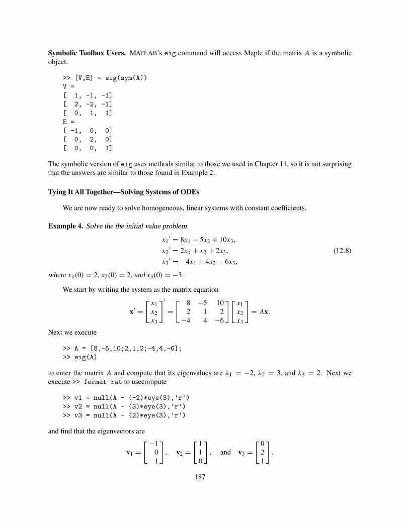
Symbolic Toolbox Users. MATLAB’s eig command will access Maple if the matrix A is a symbolicobject.

>> [V,E] = eig(sym(A))V =[ 1, -1, -1][ 2, -2, -1][ 0, 1, 1]E =[ -1, 0, 0][ 0, 2, 0][ 0, 0, 1]

The symbolic version of eig uses methods similar to those we used in Chapter 11, so it is not surprisingthat the answers are similar to those found in Example 2.

Tying It All Together—Solving Systems of ODEs

We are now ready to solve homogeneous, linear systems with constant coefficients.

Example 4. Solve the the initial value problem

x1′ = 8x1 − 5x2 + 10x3,

x2′ = 2x1 + x2 + 2x3,

x3′ = −4x1 + 4x2 − 6x3,

(12.8)

where x1(0) = 2, x2(0) = 2, and x3(0) = −3.

We start by writing the system as the matrix equation

x′ =[

x1x2x3

]′=[ 8 −5 10

2 1 2−4 4 −6

][

x1x2x3

]

= Ax.

Next we execute

>> A = [8,-5,10;2,1,2;-4,4,-6];>> eig(A)

to enter the matrix A and compute that its eigenvalues are λ1 = −2, λ2 = 3, and λ3 = 2. Next weexecute >> format rat to usecompute

>> v1 = null(A - (-2)*eye(3),'r')>> v2 = null(A - (3)*eye(3),'r')>> v3 = null(A - (2)*eye(3),'r')

and find that the eigenvectors are

v1 =[−1

01

]

, v2 =[ 1

10

]

, and v3 =[ 0

21

]

.

187

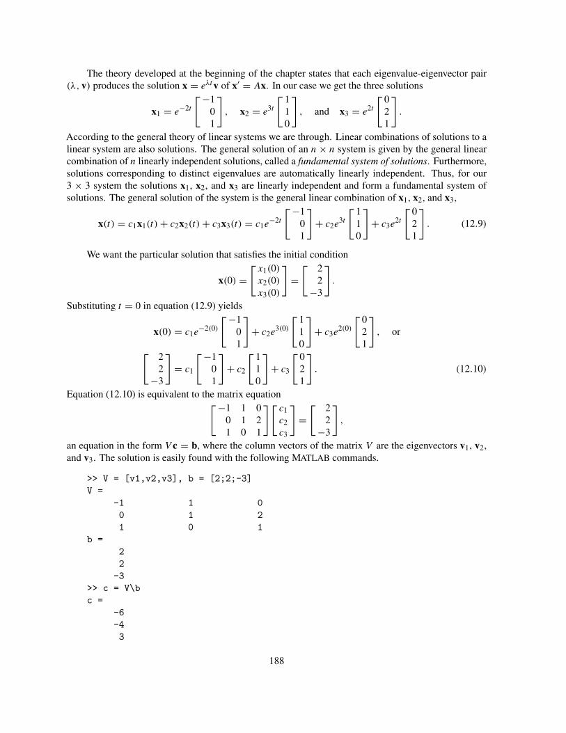
The theory developed at the beginning of the chapter states that each eigenvalue-eigenvector pair(λ, v) produces the solution x = eλtv of x′ = Ax. In our case we get the three solutions

x1 = e−2t

[−101

]

, x2 = e3t

[ 110

]

, and x3 = e2t

[ 021

]

.

According to the general theory of linear systems we are through. Linear combinations of solutions to alinear system are also solutions. The general solution of an n × n system is given by the general linearcombination of n linearly independent solutions, called a fundamental system of solutions. Furthermore,solutions corresponding to distinct eigenvalues are automatically linearly independent. Thus, for our3 × 3 system the solutions x1, x2, and x3 are linearly independent and form a fundamental system ofsolutions. The general solution of the system is the general linear combination of x1, x2, and x3,

x(t) = c1x1(t) + c2x2(t) + c3x3(t) = c1e−2t

[−101

]

+ c2e3t

[ 110

]

+ c3e2t

[ 021

]

. (12.9)

We want the particular solution that satisfies the initial condition

x(0) =[

x1(0)

x2(0)

x3(0)

]

=[ 2

2−3

]

.

Substituting t = 0 in equation (12.9) yields

x(0) = c1e−2(0)

[−101

]

+ c2e3(0)

[ 110

]

+ c3e2(0)

[ 021

]

, or

[ 22

−3

]

= c1

[−101

]

+ c2

[ 110

]

+ c3

[ 021

]

. (12.10)

Equation (12.10) is equivalent to the matrix equation[−1 1 0

0 1 21 0 1

][

c1c2c3

]

=[ 2

2−3

]

,

an equation in the form V c = b, where the column vectors of the matrix V are the eigenvectors v1, v2,and v3. The solution is easily found with the following MATLAB commands.

>> V = [v1,v2,v3], b = [2;2;-3]V =

-1 1 00 1 21 0 1

b =22

-3>> c = V\bc =

-6-43

188

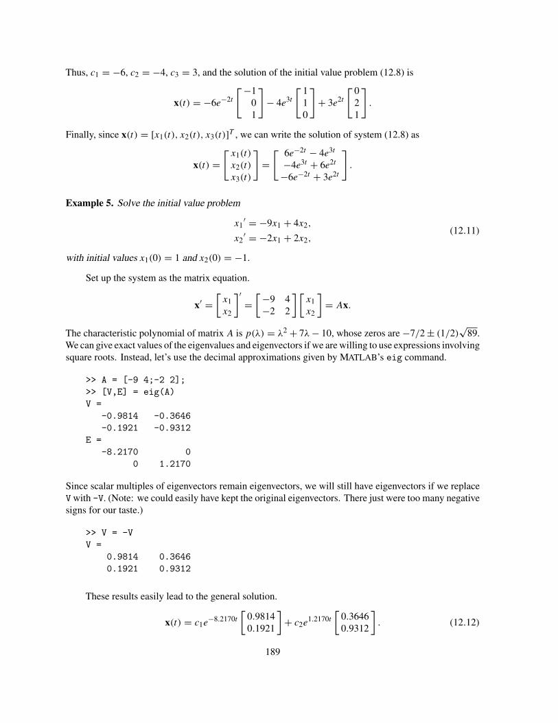
Thus, c1 = −6, c2 = −4, c3 = 3, and the solution of the initial value problem (12.8) is

x(t) = −6e−2t

[−101

]

− 4e3t

[ 110

]

+ 3e2t

[ 021

]

.

Finally, since x(t) = [x1(t), x2(t), x3(t)]T , we can write the solution of system (12.8) as

x(t) =[

x1(t)

x2(t)

x3(t)

]

=[ 6e−2t − 4e3t

−4e3t + 6e2t

−6e−2t + 3e2t

]

.

Example 5. Solve the initial value problem

x1′ = −9x1 + 4x2,

x2′ = −2x1 + 2x2,

(12.11)

with initial values x1(0) = 1 and x2(0) = −1.

Set up the system as the matrix equation.

x′ =[

x1x2

]′=[−9 4

−2 2

] [

x1x2

]

= Ax.

The characteristic polynomial of matrix A is p(λ) = λ2 + 7λ − 10, whose zeros are −7/2 ± (1/2)√

89.We can give exact values of the eigenvalues and eigenvectors if we are willing to use expressions involvingsquare roots. Instead, let’s use the decimal approximations given by MATLAB’s eig command.

>> A = [-9 4;-2 2];>> [V,E] = eig(A)V =

-0.9814 -0.3646-0.1921 -0.9312

E =-8.2170 0

0 1.2170

Since scalar multiples of eigenvectors remain eigenvectors, we will still have eigenvectors if we replaceV with -V. (Note: we could easily have kept the original eigenvectors. There just were too many negativesigns for our taste.)

>> V = -VV =

0.9814 0.36460.1921 0.9312

These results easily lead to the general solution.

x(t) = c1e−8.2170t

[

0.98140.1921

]

+ c2e1.2170t

[

0.36460.9312

]

. (12.12)

189

We need to determine the solution that satisfies the initial condition

x(0) =[

x1(0)

x2(0)

]

=[

1−1

]

.

Substituting t = 0 in equation (12.12) yields[

1−1

]

= c1

[

0.98140.1921

]

+ c2

[

0.36460.9312

]

,

which is equivalent to the matrix equation[

0.9814 0.36460.1921 0.9312

] [

c1c2

]

=[

1−1

]

.

This is an equation in the form V c = b, and is easily solved in MATLAB.

>> b = [1;-1];>> c = V\bc =

1.5356-1.3907

Therefore, the solution of the initial value problem for system (12.11) is

x(t) = 1.5356e−8.2170t

[

0.98140.1921

]

− 1.3907e1.2170t

[

0.36460.9312

]

.

Example 6. Find the general solution of the system

x1′ = 15x1 − 6x2 − 18x3 − 6x4,

x2′ = −4x1 + 5x2 + 8x3 + 4x4,

x3′ = 12x1 − 6x2 − 15x3 − 6x4,

x4′ = 4x1 − 2x2 − 8x3 − x4.

Set up the system as the matrix equation,

x′ =⎡

⎢

⎣

x1x2x3x4

⎤

⎥

⎦

′

=⎡

⎢

⎣

15 −6 −18 −6−4 5 8 412 −6 −15 −6

4 −2 −8 −1

⎤

⎥

⎦

⎡

⎢

⎣

x1x2x3x4

⎤

⎥

⎦= Ax.

Enter the matrix A into MATLAB’s workspace and compute the eigenvalues,

>> A = [15 -6 -18 -6;-4 5 8 4;12 -6 -15 -6;4 -2 -8 -1];>> E = eig(A)E =

-3.00003.00001.00003.0000

190

What sets this matrix apart from previous matrices is the presence of a repeated eigenvalue. The eigenvalue3 is an eigenvalue of multiplicity two3.

The eigenvectors associated with λ1 = −3 and λ2 = 1 are easily captured with MATLAB’s nullcommand.

>> v1 = null(A - (-3)*eye(4),'r')v1 =

1-111

>> v2 = null(A - 1*eye(4),'r')v2 =

0-101

The three equations in Example 4 required three independent eigenvectors to form the generalsolution. The two equations in Example 5 required two independent eigenvectors to form the generalsolution. In this example we have four equations, so four independent eigenvectors are required. Wehave two independent eigenvectors, but only one eigenvalue remains. Let’s cross our fingers for luck anduse MATLAB’s null command once more.

>> null(A - 3*eye(4),'r')ans =

0.5000 -1.00001.0000 0

0 -1.00000 1.0000

Fortunately for us4, the eigenspace associated with the eigenvalue λ3 = 3 has two basis vectors, exactlythe number needed to produce the general solution

x(t) = c1e−3t

⎡

⎢

⎣

1−1

11

⎤

⎥

⎦+ c2e

1t

⎡

⎢

⎣

0−1

01

⎤

⎥

⎦+ c3e

3t

⎡

⎢

⎣

1/2100

⎤

⎥

⎦+ c4e

3t

⎡

⎢

⎣

−10

−11

⎤

⎥

⎦.

3 Symbolic Toolbox users might find the sequence of commands p = poly(sym(A)); factor(p)illuminating. Does this demonstrate why 3 is an eigenvalue of multiplicity two?

4 In later sections of this chapter we will show how to form the general solution when you have fewerthan the required number of eigenvectors.

191

Complex Eigenvalues

Two key facts aid in the solution of systems involving complex eigenvalues and eigenvectors. Fore-most is Euler’s famous identity,

eiθ = cos θ + i sin θ.

Secondly, if you find a complex solution of a linear, homogeneous system with constant real coefficients,then both the real and imaginary parts of your complex solution will also be solutions of your system.

Example 7. Solve the initial value problem

x1′ = −x1 + 2x3,

x2′ = 2x1 + 3x2 − 6x3,

x3′ = −2x1 − x3,

(12.13)

where x1(0) = 4, x2(0) = −5, and x3(0) = 9.

Set up the system as the matrix equation

x′ =[

x1x2x3

]′=[−1 0 2

2 3 −6−2 0 −1

][

x1x2x3

]

= Ax.

Note that the entries of the matrix A are real numbers, so the coefficients of the characteristic polynomialmust be real numbers, which is easily checked in MATLAB.

>> A = [-1 0 2;2 3 -6;-2 0 -1];>> p = poly(A)p =

1.0000 -1.0000 -1.0000 -15.0000

If a polynomial has real coefficients, any complex zeros must occur in complex conjugate5 pairs.

>> r = roots(p)r =

3.0000-1.0000 + 2.0000i-1.0000 - 2.0000i

Note that both −1+2i and −1−2i are eigenvalues; the eigenvalues occur in conjugate pairs. Furthermore,the eigenvectors must also occur in complex conjugate pairs6. The computation of the eigenvalues of A

can be confirmed by executing

>> eig(A)ans =

3.0000-1.0000 + 2.0000i-1.0000 - 2.0000i

5 The conjugate of a + bi is a − bi.6 The conjugate of a vector or matrix is found by taking the complex conjugate of each entry. For

example, the conjugate of [1/2, −1/2 + (1/2)i, (1/2)i]T is [1/2, −1/2 − (1/2)i, −(1/2)i]T .

192

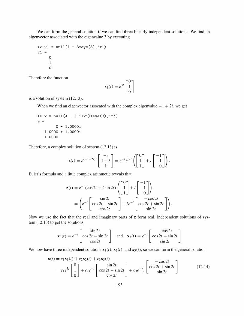
We can form the general solution if we can find three linearly independent solutions. We find aneigenvector associated with the eigenvalue 3 by executing

>> v1 = null(A - 3*eye(3),'r')v1 =

010

Therefore the function

x1(t) = e3t

[ 010

]

is a solution of system (12.13).

When we find an eigenvector assocated with the complex eigenvalue −1 + 2i, we get

>> w = null(A - (-1+2i)*eye(3),'r')w =

0 - 1.0000i1.0000 + 1.0000i1.0000

Therefore, a complex solution of system (12.13) is

z(t) = e(−1+2i)t

[ −i

1 + i

1

]

= e−t ei2t

([ 011

]

+ i

[−110

])

.

Euler’s formula and a little complex arithmetic reveals that

z(t) = e−t (cos 2t + i sin 2t)

([ 011

]

+ i

[−110

])

=(

e−t

[ sin 2t

cos 2t − sin 2t

cos 2t

]

+ ie−t

[ − cos 2t

cos 2t + sin 2t

sin 2t

])

.

Now we use the fact that the real and imaginary parts of z form real, independent solutions of sys-tem (12.13) to get the solutions

x2(t) = e−t

[ sin 2t

cos 2t − sin 2t

cos 2t

]

and x3(t) = e−t

[ − cos 2t

cos 2t + sin 2t

sin 2t

]

We now have three independent solutions x1(t), x2(t), and x3(t), so we can form the general solution

x(t) = c1x1(t) + c2x2(t) + c3x3(t)

= c1e3t

[ 010

]

+ c2e−t

[ sin 2t

cos 2t − sin 2t

cos 2t

]

+ c3e−t .

[ − cos 2t

cos 2t + sin 2t

sin 2t

]

(12.14)

193

We want the solution that satisfies the initial condition x(0) = [x1(0), x2(0), x3(0)]T = [4, −5, 9]T .Substitute t = 0 in equation (12.14) to get

[ 4−5

9

]

= c1

[ 010

]

+ c2

[ 011

]

+ c3

[−110

]

=[ 0 0 −1

1 1 10 1 0

][

c1c2c3

]

,

a matrix equation in the form Wc = b. We can solve using the MATLAB commands

>> W = [0 0 -1;1 1 1;0 1 0];>> b = [4;-5;9];>> c = W\bc =

-109

-4

Substitution of c1 = −10, c2 = 9, and c3 = −4 in equation (12.14), a little arithmetic, and we arrive atthe final solution of the initial value problem posed in equation (12.13).

[

x1(t)

x2(t)

x3(t)

]

=[

e−t (4 cos 2t + 9 sin 2t)

−10e3t + e−t (5 cos 2t − 13 sin 2t)

e−t (9 cos 2t − 4 sin 2t)

]

The Exponential of a Matrix

In order to solve systems which do not have a full complement of eigenvectors, we need a new idea.It is provided by the exponential of a matrix.

Definition. If A is a n × n matrix, then the exponential of A is defined by

eA = I + A + A2

2!+ A3

3!+ · · · + Ak

k!+ · · · , (12.15)

where I is the n × n identity matrix.

It can be shown that the infinite series (12.15) converges for every n × n matrix A. In all but a fewsimple cases, it’s quite difficult to compute the exponential of a matrix with this definition. However,diagonal matrices are always easy to work with. For example, if

D =[

a 00 b

]

,

we can compute

D2 =[

a2 00 b2

]

, D3 =[

a3 00 b3

]

, . . . , Dn =[

an 00 bn

]

.

194

Hence,

eD = I + D + 1

2!D2 + · · · ,

=[

1 00 1

]

+[

a 00 b

]

+ 1

2!

[

a2 00 b2

]

+ · · ·

=[

1 + a + 12!a

2 + · · · 00 1 + b + 1

2!b2 + · · ·

]

=[

ea 00 eb

]

While this calculation was for a 2 × 2 diagonal matrix, a similar calculation demonstrates that theexponential of a diagonal matrix of any size is equal to the diagonal matrix found by exponentiating thediagonal entries of the original matrix.

Example 8. If I is the n × n identity matrix and r is a scalar (number), prove that erI = erI.

Since rI is the diagonal matrix with all diagonal entries equal to r , the result is immediate from theprevious computation. For example,

e3I = e3I = e3[

1 00 1

]

=[

e3 00 e3

]

.

You can easily check this result with MATLAB’s expm command7. Note that e3 ≈ 20.0855.

>> I = eye(2);>> E = expm(3*I)E =

20.0855 00 20.0855

Properties of the exponential of a matrix. The most important property of the exponential function isthe formula ea+b = eaeb. We should ask if this formula remains true for the exponential of a matrix.

Proposition 1. If the matrices A and B commute, i.e., if AB = BA, then

eA+B = eAeB.

7 It is important to note that exp(3*eye(2)) gives an incorrect result, since exp is array smart andcomputes the exponential of each entry of the matrix. Try it! The command expm is one command inMATLAB which is not array smart. Instead expm is matrix smart, and it must be used when computingthe exponential of a matrix. Symbolic Toolbox users will want to try expm(3*sym(eye(2))).

195

For example, note that A = [1,2;-1,0] and B = [0,-2;1,1] commute (enter A*B and B*A andcompare). Compute

>> expm(A + B)ans =

2.7183 00 2.7183

>> expm(A)*expm(B)ans =

2.7183 00 2.7183

to verify that eA+B = eAeB for these particular matrices A and B. However, matricesC = [1,1;1,1] and D = [1,2;3,4] do not commute (Check this with C*D and D*C.). Use MATLABto show that eC+D �= eCeD .

Another property that we will find extremely useful is the following.

Proposition 2. If A is an n × n matrix, then the derivative of etA is given as

d

dtetA = AetA.

We end this section with a powerful theorem. One of the first initial value problems encounteredin a course on ordinary differential equations is x′ = ax, x(0) = x0. It is easy to show (separate thevariables) that the solution of this initial value problem is x = eatx0. One would hope that a similarresult applies to the matrix equation x′ = Ax, x(0) = x0.

Theorem 1. Let x′ = Ax be the matrix equation representing a system of n first order, linear, ho-mogeneous differential equations with constant coefficients. The solution of the initial value problem,x′ = Ax, x(0) = x0, is

x(t) = eAtx0.

Readers can easily prove this theorem by direct substitution and the application of Proposition 2.The initial condition is easily verified using the result developed in Example 8.

Symbolic Toolbox Users. Owners of the Symbolic Toolbox can readily check the validity of this lastproposition for the matrix A = [1,-1;-1,1].

>> syms t>> A = sym([1,-1;-1,1]);>> diff(expm(t*A),t)ans =[ exp(2*t), -exp(2*t)][ -exp(2*t), exp(2*t)]>> A*expm(t*A)ans =[ exp(2*t), -exp(2*t)][ -exp(2*t), exp(2*t)]

196

Note that the results are identical, showing that ddt

etA = AetA for this particular matrix A. Experiment!Convince yourself that d

dtetA = AetA for other square matrices A. Try a 3 × 3 matrix.

In Example 4, we used eigenvalues and eigenvectors to show that the solution of the system

[

x1x2x3

]′=[ 8 −5 10

2 1 2−4 4 −6

][

x1x2x3

]

,

with initial condition x0 = [2, 2, −3]T , was

[

x1(t)

x2(t)

x3(t)

]

=[ 6e−2t − 4e3t

−4e3t + 6e2t

−6e−2t + 3e2t

]

.

Let’s use Theorem 1 to produce the same result.

>> syms t>> A = [8 -5 10;2 1 2;-4 4 -6];>> x0 = sym([2;2;-3]);>> x = expm(A*t)*x0x =[ 6*exp(-2*t)-4*exp(3*t)][ 6*exp(2*t)-4*exp(3*t)][ 3*exp(2*t)-6*exp(-2*t)]

This is a startling result, clearly demonstrating the power of the exponential matrix.

Solving Systems with Repeated Eigenvalues

We have shown how to solve the system x′ = Ax when the eigenvalues of A are distinct. The matrixA in Example 6 had a repeated eigenvalue, but it still had a full complement of eigenvectors, and thatallowed us to complete the solution. However, if the matrix A is n×n and there are fewer than n linearlyindependent eigenvectors, then the level of difficulty is raised an order or two in magnitude.

The problem. The following example is typical of 2 × 2 systems with only one eigenvalue.

Example 9. Find the solution of the initial value problem

x1′ = 13x1 + 11x2,

x2′ = −11x1 − 9x2,

(12.16)

with initial conditions x1(0) = 1 and x2(0) = 2.

197

System (12.16) has the matrix form

x′ =[

x1x2

]′=[

13 11−11 −9

] [

x1x2

]

= Ax, (12.17)

with initial condition x(0) = [1, 2]T . It is easily verified (try poly(A)) that the characteristic polynomialis p(λ) = λ2 − 4λ + 4 = (λ − 2)2, indicating that A has an eigenvalue λ = 2 of algebraic multiplicitytwo. Difficulties become immediately apparent when we execute the command

>> null(A - 2*eye(2),'r')ans =

-11

showing that, up to multiplication by a constant, v1 = [−1, 1]T is the only eigenvector. We need twoindependent solutions to form the general solution of system (12.16), but we only have one.

We need some terminology to describe this phenomenon.

Definition. If λj is an eigenvalue of the matrix A, we define the algebraic multiplicity of λj to be thelargest power of (λ − λj ) which divides the characteristic polynomial of A. We define the geometricmultiplicity of λj to be the dimension of the nullspace of A − λj I , i.e. the dimension of the eigenspaceassociated to λj .

It can be shown that the geometric multiplicity is never larger than the algebraic multiplicity. In thecase of system (12.17), the geometric multiplicity (one) of the eigenvalue λ = 2 is strictly smaller thanits algebraic multiplicity (two). Comparison of Examples 6 and 9 show that we have a problem preciselywhen the geometric multiplicity is smaller than the algebraic multiplicity.

Solving systems with only one eigenvalue. We will complete the solution of Example 9 by computingetA for the matrix A in (12.17). To do so, we notice that tA = 2tI + t (A − 2I ). Furthermore, since theidentity matrix commutes with every other matrix, the matrices 2tI and t (A − 2I ) commute. Hence, wecan use Proposition 1 and the identity developed in Example 8 to write

etA = e2tI+t (A−2I ) = e2tI et (A−2I ) = e2t I et (A−2I ) = e2t et (A−2I ). (12.18)

Using the definition of the exponential of a matrix in equation (12.18) to compute the second exponential,we get

etA = e2t

(

I + t (A − 2I ) + t2

2!(A − 2I )2 + t3

3!(A − 2I )3 + · · ·

)

(12.19)

For this matrix we get a break, since λ = 2 is the only eigenvalue of the 2 × 2 matrix A. It can be shownif an n × n matrix A has only one eigenvalue λ, then (A − λI)n is the zero matrix8. We can verify thisin this case by executing

>> (A - 2*eye(2))^2ans =

0 00 0

8 This is not easy. See Exercises 54–57

198

Therefore, in (12.19), the powers (A − 2I )k = 0 for all k ≥ 2 and the series truncates after two terms,leaving

etA = e2t (I + t (A − 2I )) ,

= e2t

{[

1 00 1

]

+ t

([

13 11−11 −9

]

− 2

[

1 00 1

])}

,

= e2t

[

1 + 11t 11t

−11t 1 − 11t

]

.

According to Theorem 1, the solution of system (12.17), with initial condition x(0) = [1, 2]T , isgiven by x(t) = etA x(0). Thus,

x(t) = etA x(0),

= e2t

([

1 + 11t 11t

−11t 1 − 11t

]) [

12

]

,

= e2t

[

1 + 33t

2 − 33t

]

.

Symbolic Toolbox Users. Owners of the Symbolic Toolbox can easily check this last solution.

>> syms t>> A = sym([13 11;-11 -9]);>> x0 = sym([1;2]);>> x = expm(t*A)*x0x =[ exp(2*t)+33*t*exp(2*t)][ -33*t*exp(2*t)+2*exp(2*t)]

For the system (12.17) we were able to actually compute the exponential of the matrix tA. It is rarethat this is so easy, but the method we used works for any 2 by 2 matrix which has a single eigenvalue λ

of multiplicity 2. In such a case we always have

etA = eλt (I + t (A − λI)) ,

and the solution to the initial value problem is given by

x(t) = etA x0 = eλt (I + t (A − λI)) x0.

More generally, the method works for an n × n system as long as the matrix has only one eigenvalue ofalgebraic multiplicity n. In such a case, the argument leading to (12.19) yields

etA = eλt

(

I + t (A − λI) + t2

2!(A − λI)2 + t3

3!(A − λI)3 + · · ·

)

= eλt

(

I + t (A − λI) + t2

2!(A − λI)2 + t3

3!(A − λI)3 + · · · + tn−1

(n − 1)!(A − λI)n−1

)

,

since (A − λI)k = 0 for k ≥ n.

199

Example 10. Find the solution of the initial value problem

x1′ = 3x1 + 3x2 + x3

x2′ = −7x1 − 6x2 − x3

x3′ = −x1 − x2 − 3x3,

(12.20)

with initial conditions x1(0) = x2(0) = x3(0) = 1.

System (12.20) has matrix form

x′ =[

x1x2x3

]′=[ 3 3 1

−7 −6 −1−1 −1 −3

][

x1x2x3

]

= Ax,

with initial condition x(0) = [1, 1, 1]T . Matrix A has a single eigenvalue with algebraic multiplicity 3.

>> A=[3 3 1; -7 -6 -1; -1 -1 -3]; p=factor(poly(sym(A)))p =(x+2)^3

Hence, (A + 2I )3 = 0 (check this) and the series expansion for etA truncates.

etA = e−2t

(

I + t (A + 2I ) + t2

2!(A + 2I )2

)

= e−2t

([ 1 0 00 1 00 0 1

]

+ t

[ 5 3 1−7 −4 −1−1 −1 −1

]

+ t2

2!

[ 3 2 1−6 −4 −2

3 2 1

])

,

Simplifying,

etA = e−2t

[ 1 + 5t + (3/2)t2 3t + t2 t + (1/2)t2

−7t − 3t2 1 − 4t − 2t2 −t − t2

−t + (3/2)t2 −t + t2 1 − t + (1/2)t2

]

.

Finally, the solution to the initial value problem is found by computing

x = etAx0 = e−2t

[ 1 + 5t + (3/2)t2 3t + t2 t + (1/2)t2

−7t − 3t2 1 − 4t − 2t2 −t − t2

−t + (3/2)t2 −t + t2 1 − t + (1/2)t2

][ 111

]

.

Thus,

x =[

x1x2x3

]

=[

e−2t (1 + 9t + 3t2)

e−2t (1 − 12t − 6t2)

e−2t (1 − 3t + 3t2)

]

.

The most general case. Our first example will point the way to the general method of solution.

Example 11. Find a fundamental set of solutions to x′ = Ax, where

A =[ 1 0 1

−6 −1 −3−6 1 −5

]

.

200

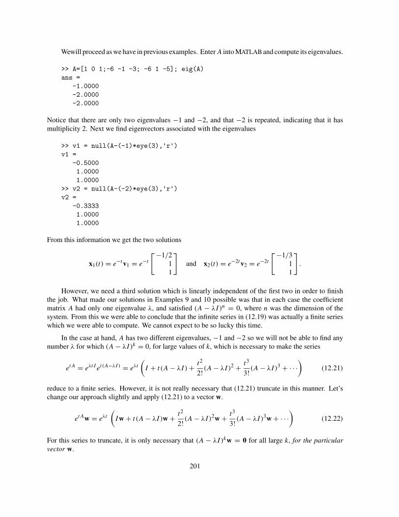
Wewill proceed as we have in previous examples. Enter A into MATLAB and compute its eigenvalues.

>> A=[1 0 1;-6 -1 -3; -6 1 -5]; eig(A)ans =

-1.0000-2.0000-2.0000

Notice that there are only two eigenvalues −1 and −2, and that −2 is repeated, indicating that it hasmultiplicity 2. Next we find eigenvectors associated with the eigenvalues

>> v1 = null(A-(-1)*eye(3),'r')v1 =

-0.50001.00001.0000

>> v2 = null(A-(-2)*eye(3),'r')v2 =

-0.33331.00001.0000

From this information we get the two solutions

x1(t) = e−tv1 = e−t

[−1/211

]

and x2(t) = e−2tv2 = e−2t

[−1/311

]

.

However, we need a third solution which is linearly independent of the first two in order to finishthe job. What made our solutions in Examples 9 and 10 possible was that in each case the coefficientmatrix A had only one eigenvalue λ, and satisfied (A − λI)n = 0, where n was the dimension of thesystem. From this we were able to conclude that the infinite series in (12.19) was actually a finite serieswhich we were able to compute. We cannot expect to be so lucky this time.

In the case at hand, A has two different eigenvalues, −1 and −2 so we will not be able to find anynumber λ for which (A − λI)k = 0, for large values of k, which is necessary to make the series

etA = eλtI et (A−λI) = eλt

(

I + t (A − λI) + t2

2!(A − λI)2 + t3

3!(A − λI)3 + · · ·

)

(12.21)

reduce to a finite series. However, it is not really necessary that (12.21) truncate in this manner. Let’schange our approach slightly and apply (12.21) to a vector w.

etAw = eλt

(

Iw + t (A − λI)w + t2

2!(A − λI)2w + t3

3!(A − λI)3w + · · ·

)

(12.22)

For this series to truncate, it is only necessary that (A − λI)kw = 0 for all large k, for the particularvector w.

201

Perhaps we can take advantage of this. Since the eigenvalue −2 has multiplicity 2, we might beable to find a vector w which is not a multiple of v2 and satisfies (A − (−2)I )2w = 0. We compute thenullspace of (A − (−2)I )2 with

>> null((A - (-2)*eye(3))^2,'r')ans =

-0.3333 01.0000 0

0 1.0000

We are in luck! The nullspace of (A − (−2)I )2 has dimension 2, with the indicated vectors as a basis.Let’s take v3 = [0, 0, 1]T , the simplest vector in this space which is not a multiple of v2.9 Using (12.21)we see that the solution with this initial value is10

x3(t) = etAv3 = e−2t (v3 + t (A − (−2)I )v3)

= e−2t

([ 001

]

+ t

[ 1−3−3

])

= e−2t

[

t

−3t

1 − 3t

]

.

The three solutions, x1, x2, and x3 form a fundamental set of solutions, and we are finished.

Generalized eigenvectors and solutions. The key to finding the third solution in Example 11 was findingthe vector v3 which satisfied (A − (−2)I )2v3 = 0. Let’s give such vectors a name.

Definition. Suppose λ is an eigenvalue of the matrix A. Any vector w which satisfies (A − λI)k w = 0for some integer k is called a generalized eigenvector associated with the eigenvalue λ.

The fact is that there are always enough generalized eigenvectors to find a basis for solutions. Wewill state this result as a theorem.

Theorem 2. Suppose A is a matrix and λ is an eigenvalue of algebraic multiplicity d. Then there is aninteger k ≤ d such that the set of all generalized eigenvectors associated to λ is equal to the nullspace of(A − λI)k and has dimension equal to d, the algebraic multiplicity of λ.

In Example 9, we found that (A − 2I )2 = 0. This meant that every 2-vector was a generalizedeigenvector associated to the eigenvalue 2. It was the fact that every vector was a generalized eigenvectorthat made things so easy in that case.

As a result of Theorem 2, we see that if λ is an eigenvalue of algebraic multiplicity d, then wecan find d linearly independent solutions. Since the sum of the algebraic multiplicities is equal to the

9 Any vector which is not a multiple of v2 would do. Taking the simplest one makes the computationseasier.

10 We use MATLAB to compute that (A − (−2)I )v3 = [1, −3, −3]T .

202

dimension of the system, we have found a method for finding the general solution which works for allsystems. Let’s summarize the method.

Procedure for solving x′ = Ax.

• Find the eigenvalues of A.• For each eigenvalue λ:

• Find the algebraic multiplicity d.

• Find the smallest integer k for which the nullspace of (A − λI)k has dimension d.

• Find a basis v1, v2, . . . , vd of the nullspace of (A − λI)k .• For j = 1, 2, . . . , d set

xj (t) = etAvj

= eλt

[

vj + t (A − λI)vj + t2

2!(A − λI)2vj + t3

3!(A − λI)3vj + · · ·

+ tk−1

(k − 1)!(A − λI)k−1vj

]

(12.23)

• If λ is complex, the real and imaginary parts of xj will be real solutions.

This procedure will result in sufficiently many linearly independent solutions to generate the generalsolution.

We will do one final example illustrating the procedure.

Example 12. Solve the initial value problem

x1′ = 3x1 − 3x2 − 6x3 + 5x4,

x2′ = −3x1 + 2x2 + 5x3 − 4x4,

x3′ = 2x1 − 6x2 − 4x3 + 7x4,

x4′ = −3x1 + 5x3 − 2x4,

(12.24)

where x1(0) = 2, x2(0) = −1, x3(0) = 0, and x4(0) = 0.

Our system can be written as x′ = Ax, where

A =⎡

⎢

⎣

3 −3 −6 5−3 2 5 −4

2 −6 −4 7−3 0 5 −2

⎤

⎥

⎦.

The first step is to use eig to compute the eigenvalues.

>> A = [3 -3 -6 5;-3 2 5 -4;2 -6 -4 7;-3 0 5 -2];>> E = eig(A)E =-1.0000 + 0.0000i-1.0000 - 0.0000i-1.00002.0000

203

We suspect roundoff error and conjecture that −1 is an eigenvalue of multiplicity 3. If the SymbolicToolbox is available, this is confirmed by the command

>> eig(sym(A))ans =[ 2][-1][-1][-1]

Thus, we see that A has two different eigenvalues, −1 and 2, with algebraic multiplicities 3 and 1,respectively11.

Let’s start with the difficult eigenvalue λ1 = −1, which has mulitplicity 3. We will use null tocompute nullspaces of powers of A − λ1I = A + I . It will be convenient to use I = eye(4);. Then

>> null(A + I,'r')ans =

-21

-11

We see that although −1 is an eigenvalue of algebraic multiplicity 3, the eigenspace has dimension 1.Thus the eigenvalue −1 has geometric multiplicity 1.

The next step is to find the integer k for which the nullspace of (A + I )k has dimension 3. We doso by computing the nullspaces of increasing powers of A + I . First,

>> null((A + I)^2,'r')ans =

2 00 11 00 1

shows that the dimension has increased to 2. However, we want the dimension to be 3, so we compute

>> null((A + I)^3,'r')ans =

1 0 00 0 10 1 00 0 1

This time the dimension is 3, the same as the algebraic multiplicity, so k = 3 and we are in business.

11 Owners of the Symbolic Toolbox can further confirm the algebraic multiplicity of the eigenvalueswith ps = poly(sym(A)), factor(ps).

204

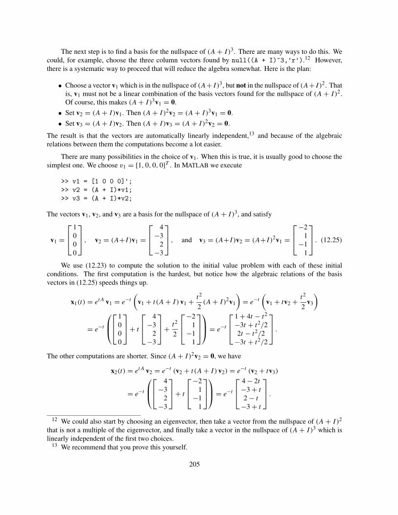
The next step is to find a basis for the nullspace of (A + I )3. There are many ways to do this. Wecould, for example, choose the three column vectors found by null((A + I)^3,'r').12 However,there is a systematic way to proceed that will reduce the algebra somewhat. Here is the plan:

• Choose a vector v1 which is in the nullspace of (A+I )3, but not in the nullspace of (A+I )2. Thatis, v1 must not be a linear combination of the basis vectors found for the nullspace of (A + I )2.Of course, this makes (A + I )3v1 = 0.

• Set v2 = (A + I )v1. Then (A + I )2v2 = (A + I )3v1 = 0.

• Set v3 = (A + I )v2. Then (A + I )v3 = (A + I )2v2 = 0.

The result is that the vectors are automatically linearly independent,13 and because of the algebraicrelations between them the computations become a lot easier.

There are many possibilities in the choice of v1. When this is true, it is usually good to choose thesimplest one. We choose v1 = [1, 0, 0, 0]T . In MATLAB we execute

>> v1 = [1 0 0 0]';>> v2 = (A + I)*v1;>> v3 = (A + I)*v2;

The vectors v1, v2, and v3 are a basis for the nullspace of (A + I )3, and satisfy

v1 =⎡

⎢

⎣

1000

⎤

⎥

⎦, v2 = (A+I )v1 =

⎡

⎢

⎣

4−3

2−3

⎤

⎥

⎦, and v3 = (A+I )v2 = (A+I )2v1 =

⎡

⎢

⎣

−21

−11

⎤

⎥

⎦. (12.25)

We use (12.23) to compute the solution to the initial value problem with each of these initialconditions. The first computation is the hardest, but notice how the algebraic relations of the basisvectors in (12.25) speeds things up.

x1(t) = etA v1 = e−t

(

v1 + t (A + I ) v1 + t2

2(A + I )2v1

)

= e−t

(

v1 + tv2 + t2

2v3

)

= e−t

⎛

⎜

⎝

⎡

⎢

⎣

1000

⎤

⎥

⎦+ t

⎡

⎢

⎣

4−3

2−3

⎤

⎥

⎦+ t2

2

⎡

⎢

⎣

−21

−11

⎤

⎥

⎦

⎞

⎟

⎠= e−t

⎡

⎢

⎣

1 + 4t − t2

−3t + t2/22t − t2/2

−3t + t2/2

⎤

⎥

⎦.

The other computations are shorter. Since (A + I )2v2 = 0, we have

x2(t) = etA v2 = e−t (v2 + t (A + I ) v2) = e−t (v2 + tv3)

= e−t

⎛

⎜

⎝

⎡

⎢

⎣

4−3

2−3

⎤

⎥

⎦+ t

⎡

⎢

⎣

−21

−11

⎤

⎥

⎦

⎞

⎟

⎠= e−t

⎡

⎢

⎣

4 − 2t

−3 + t

2 − t

−3 + t

⎤

⎥

⎦.

12 We could also start by choosing an eigenvector, then take a vector from the nullspace of (A + I )2

that is not a multiple of the eigenvector, and finally take a vector in the nullspace of (A + I )3 which islinearly independent of the first two choices.

13 We recommend that you prove this yourself.

205

Finally, since (A + I )v3 = 0, v3 is an eigenvector, and

x3(t) = etA v3 = e−t v3 = e−t

⎡

⎢

⎣

−21

−11

⎤

⎥

⎦.

Thus, we have found three linearly independent solutions corresponding to the eigenvalue λ1 = −1,which has algebraic multiplicity three. We get one more in the usual way from the eigenvalue λ2 = 2,which has algebraic multiplicity 1.

v4 = null(A - 2*I,'r')v4 =

-0.50000.50000.50001.0000

The solution, x4, to the initial value problem with initial value x4(0) = v4 is

x4(t) = etA v4 = e2t v4 = e2t

⎡

⎢

⎣

−1/21/21/2

1

⎤

⎥

⎦.

Having found four linearly independent solutions, linearity allows us to form the general solutionof system (12.24) by forming a linear combination of our basic solutions.

x(t) = c1x1(t) + c2x2(t) + c3x3(t) + c4x4(t) (12.26)

To solve the initial value problem with x(0) = x0 = [2, −1, 0, 0]T , we must substitute t = 0 inequation (12.26).

x(0) = c1x1(0) + c2x2(0) + c3x3(0) + c4x4(0)

x0 = c1v1 + c2v2 + c3v3 + c4v4

Of course, this is equivalent to the matrix equation

x0 = [v1, v2, v3, v4]

⎡

⎢

⎣

c1c2c3c4

⎤

⎥

⎦,

so we can find the solution with the following MATLAB code

>> V = [v1 v2 v3 v4];>> x0 = [2;-1;0;0];>> c = V\x0c =

5.00003.00007.00002.0000

206

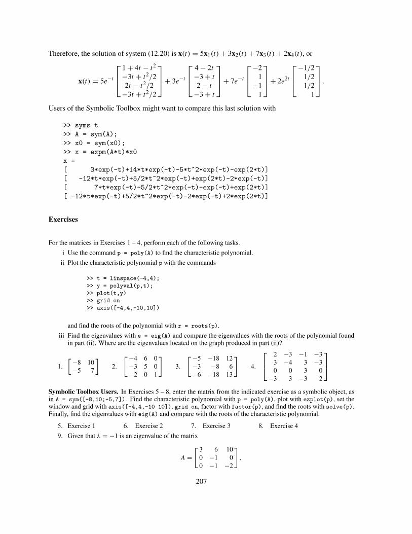
Therefore, the solution of system (12.20) is x(t) = 5x1(t) + 3x2(t) + 7x3(t) + 2x4(t), or

x(t) = 5e−t

⎡

⎢

⎣

1 + 4t − t2

−3t + t2/22t − t2/2

−3t + t2/2

⎤

⎥

⎦+ 3e−t

⎡

⎢

⎣

4 − 2t

−3 + t

2 − t

−3 + t

⎤

⎥

⎦+ 7e−t

⎡

⎢

⎣

−21

−11

⎤

⎥

⎦+ 2e2t

⎡

⎢

⎣

−1/21/21/2

1

⎤

⎥

⎦.

Users of the Symbolic Toolbox might want to compare this last solution with

>> syms t>> A = sym(A);>> x0 = sym(x0);>> x = expm(A*t)*x0x =[ 3*exp(-t)+14*t*exp(-t)-5*t^2*exp(-t)-exp(2*t)][ -12*t*exp(-t)+5/2*t^2*exp(-t)+exp(2*t)-2*exp(-t)][ 7*t*exp(-t)-5/2*t^2*exp(-t)-exp(-t)+exp(2*t)][ -12*t*exp(-t)+5/2*t^2*exp(-t)-2*exp(-t)+2*exp(2*t)]

Exercises

For the matrices in Exercises 1 – 4, perform each of the following tasks.

i Use the command p = poly(A) to find the characteristic polynomial.

ii Plot the characteristic polynomial p with the commands

>> t = linspace(-4,4);

>> y = polyval(p,t);

>> plot(t,y)

>> grid on

>> axis([-4,4,-10,10])

and find the roots of the polynomial with r = roots(p).

iii Find the eigenvalues with e = eig(A) and compare the eigenvalues with the roots of the polynomial foundin part (ii). Where are the eigenvalues located on the graph produced in part (ii)?

1.

[−8 10−5 7

]

2.

[−4 6 0−3 5 0−2 0 1

]

3.

[−5 −18 12−3 −8 6−6 −18 13

]

4.

⎡

⎢

⎣

2 −3 −1 −33 −4 3 −30 0 3 0

−3 3 −3 2

⎤

⎥

⎦

Symbolic Toolbox Users. In Exercises 5 – 8, enter the matrix from the indicated exercise as a symbolic object, asin A = sym([-8,10;-5,7]). Find the characteristic polynomial with p = poly(A), plot with ezplot(p), set thewindow and grid with axis([-4,4,-10 10]), grid on, factor with factor(p), and find the roots with solve(p).Finally, find the eigenvalues with eig(A) and compare with the roots of the characteristic polynomial.

5. Exercise 1 6. Exercise 2 7. Exercise 3 8. Exercise 4

9. Given that λ = −1 is an eigenvalue of the matrix

A =[ 3 6 10

0 −1 00 −1 −2

]

,

207

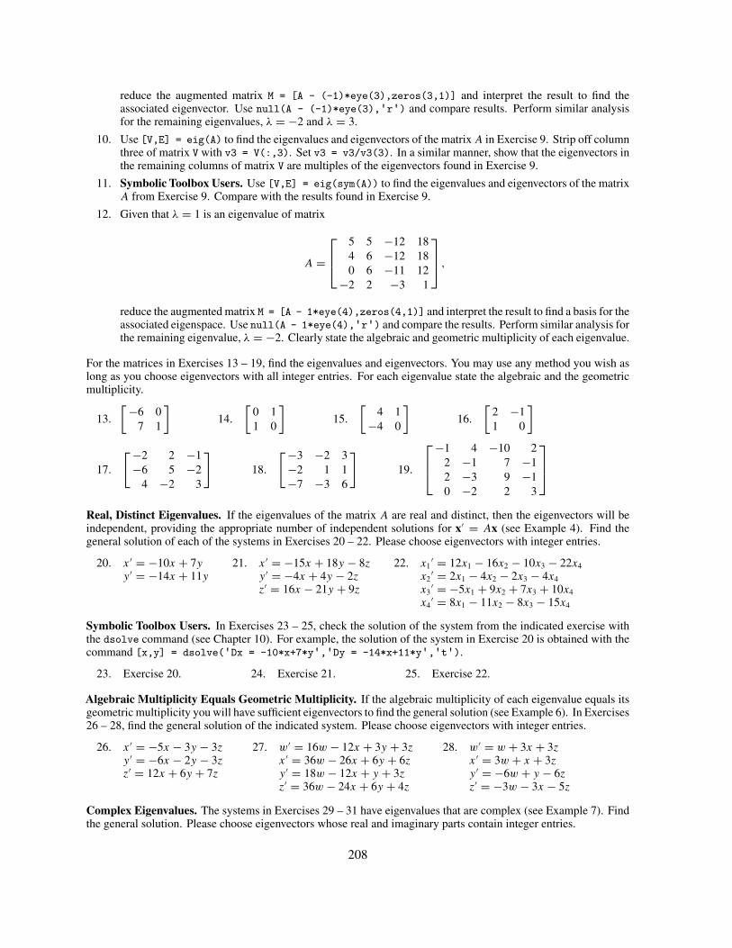
reduce the augmented matrix M = [A - (-1)*eye(3),zeros(3,1)] and interpret the result to find theassociated eigenvector. Use null(A - (-1)*eye(3),'r') and compare results. Perform similar analysisfor the remaining eigenvalues, λ = −2 and λ = 3.

10. Use [V,E] = eig(A) to find the eigenvalues and eigenvectors of the matrix A in Exercise 9. Strip off columnthree of matrix V with v3 = V(:,3). Set v3 = v3/v3(3). In a similar manner, show that the eigenvectors inthe remaining columns of matrix V are multiples of the eigenvectors found in Exercise 9.

11. Symbolic Toolbox Users. Use [V,E] = eig(sym(A)) to find the eigenvalues and eigenvectors of the matrixA from Exercise 9. Compare with the results found in Exercise 9.

12. Given that λ = 1 is an eigenvalue of matrix

A =⎡

⎢

⎣

5 5 −12 184 6 −12 180 6 −11 12

−2 2 −3 1

⎤

⎥

⎦,

reduce the augmented matrix M = [A - 1*eye(4),zeros(4,1)] and interpret the result to find a basis for theassociated eigenspace. Use null(A - 1*eye(4),'r') and compare the results. Perform similar analysis forthe remaining eigenvalue, λ = −2. Clearly state the algebraic and geometric multiplicity of each eigenvalue.

For the matrices in Exercises 13 – 19, find the eigenvalues and eigenvectors. You may use any method you wish aslong as you choose eigenvectors with all integer entries. For each eigenvalue state the algebraic and the geometricmultiplicity.

13.

[−6 07 1

]

14.

[

0 11 0

]

15.

[

4 1−4 0

]

16.

[

2 −11 0

]

17.

[−2 2 −1−6 5 −2

4 −2 3

]

18.

[−3 −2 3−2 1 1−7 −3 6

]

19.

⎡

⎢

⎣

−1 4 −10 22 −1 7 −12 −3 9 −10 −2 2 3

⎤

⎥

⎦

Real, Distinct Eigenvalues. If the eigenvalues of the matrix A are real and distinct, then the eigenvectors will beindependent, providing the appropriate number of independent solutions for x′ = Ax (see Example 4). Find thegeneral solution of each of the systems in Exercises 20 – 22. Please choose eigenvectors with integer entries.

20. x ′ = −10x + 7yy ′ = −14x + 11y

21. x ′ = −15x + 18y − 8zy ′ = −4x + 4y − 2zz′ = 16x − 21y + 9z

22. x1′ = 12x1 − 16x2 − 10x3 − 22x4

x2′ = 2x1 − 4x2 − 2x3 − 4x4

x3′ = −5x1 + 9x2 + 7x3 + 10x4

x4′ = 8x1 − 11x2 − 8x3 − 15x4

Symbolic Toolbox Users. In Exercises 23 – 25, check the solution of the system from the indicated exercise withthe dsolve command (see Chapter 10). For example, the solution of the system in Exercise 20 is obtained with thecommand [x,y] = dsolve('Dx = -10*x+7*y','Dy = -14*x+11*y','t').

23. Exercise 20. 24. Exercise 21. 25. Exercise 22.

Algebraic Multiplicity Equals Geometric Multiplicity. If the algebraic multiplicity of each eigenvalue equals itsgeometric multiplicity you will have sufficient eigenvectors to find the general solution (see Example 6). In Exercises26 – 28, find the general solution of the indicated system. Please choose eigenvectors with integer entries.

26. x ′ = −5x − 3y − 3zy ′ = −6x − 2y − 3zz′ = 12x + 6y + 7z

27. w′ = 16w − 12x + 3y + 3zx ′ = 36w − 26x + 6y + 6zy ′ = 18w − 12x + y + 3zz′ = 36w − 24x + 6y + 4z

28. w′ = w + 3x + 3zx ′ = 3w + x + 3zy ′ = −6w + y − 6zz′ = −3w − 3x − 5z

Complex Eigenvalues. The systems in Exercises 29 – 31 have eigenvalues that are complex (see Example 7). Findthe general solution. Please choose eigenvectors whose real and imaginary parts contain integer entries.

208

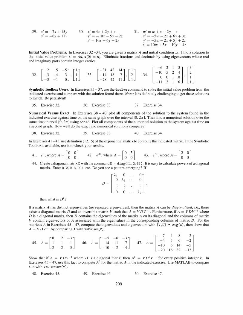
29. x ′ = −7x + 15yy ′ = −6x + 11y

30. x ′ = 4x + 2y + zy ′ = −10x − 5y − 2zz′ = 10x + 6y + 2z

31. w′ = w + x − 2y − zx ′ = −5w − 2x + 6y + 3zy ′ = −5w − 2x + 5y + 2zz′ = 10w + 5x − 10y − 4z

Initial Value Problems. In Exercises 32 –34, you are given a matrix A and initial condition x0. Find a solution tothe initial value problem x′ = Ax, x(0) = x0. Eliminate fractions and decimals by using eigenvectors whose realand imaginary parts contain integer entries.

32.

[ 2 5 −5−3 −4 3−3 −1 0

]

,

[ 111

]

33.

[−31 42 14−14 18 7−28 42 11

]

,

[ 121

]

34.

⎡

⎢

⎣

−6 2 1 3−10 5 2 4

0 0 1 0−11 2 1 6

⎤

⎥

⎦,

⎡

⎢

⎣

3211

⎤

⎥

⎦

Symbolic Toolbox Users. In Exercises 35 – 37, use the dsolve command to solve the initial value problem from theindicated exercise and compare with the solution found there. Note: It is definitely challenging to get these solutionsto match. Be persistent!

35. Exercise 32. 36. Exercise 33. 37. Exercise 34.

Numerical Versus Exact. In Exercises 38 – 40, plot all components of the solution to the system found in theindicated exercise against time on the same graph over the interval [0, 2π ]. Then find a numerical solution over thesame time interval [0, 2π ] using ode45. Plot all components of the numerical solution to the system against time ona second graph. How well do the exact and numerical solutions compare?

38. Exercise 32. 39. Exercise 33. 40. Exercise 34.

In Exercises 41 – 43, use definition (12.15) of the exponential matrix to compute the indicated matrix. If the SymbolicToolboxis available, use it to check your results.

41. eA, where A =[

0 00 0

]

42. eAt , where A =[

0 50 0

]

43. eAt , where A =[

2 00 3

]

44. Create a diagonal matrix Dwith the command D = diag([1,2,3]). It is easy to calculate powers of a diagonalmatrix. Enter D^2, D^3, D^4, etc. Do you see a pattern emerging? If

D =

⎡

⎢

⎢

⎣

λ1 0 · · · 00 λ2 · · · 0...

.... . .

...

0 0 · · · λn

⎤

⎥

⎥

⎦

,

then what is Dk?

If a matrix A has distinct eigenvalues (no repeated eigenvalues), then the matrix A can be diagonalized; i.e., thereexists a diagonal matrix D and an invertible matrix V such that A = V DV −1. Furthermore, if A = V DV −1 whereD is a diagonal matrix, then D contains the eigenvalues of the matrix A on its diagonal and the columns of matrixV contain eigenvectors of A associated with the eigenvalues in the corresponding columns of matrix D. For thematrices A in Exercises 45 – 47, compute the eigenvalues and eigenvectors with [V,D] = eig(A), then show thatA = V DV −1 by comparing A with V*D*inv(V).

45. A =[ 0 2 −3

1 1 12 −2 5

]

46. A =[ −5 −6 −3

14 11 7−10 −2 −4

]

47. A =⎡

⎢

⎣

−7 4 8 −2−4 5 6 −2

−10 6 14 −5−20 16 32 −13

⎤

⎥

⎦

Show that if A = V DV −1 where D is a diagonal marix, then Ak = V DkV −1 for every positive integer k. InExercises 45 – 47, use this fact to compute A5 for the matrix A in the indicated exercise. Use MATLAB to compareA^5 with V*D^5*inv(V).

48. Exercise 45. 49. Exercise 46. 50. Exercise 47.

209

Show that if A = V DV −1 where D is a diagonal marix, then eA = V eDV −1. (Hint: Use use the previous threeexercises and equation (12.15)). Further, show that etA = V etDV −1 and use this result to calculate etA for thematrices in Exercises 51 – 53. If the Symbolic Toolbox available, check the result with expm(t*A).

51. A =[−3 4

−2 3

]

52. A =[−8 9

−6 7

]

53. A =[

8 6−12 −10

]

The Cayley-Hamilton theorem states that every matrix must satisfy its characteristic polynomial pA. For example,the characteristic polynomial of

A =[ 5 −5 3

2 −1 20 1 2

]

is pA(λ) = λ3 − 6λ2 + 11λ − 6. The following commands will verify that pA(A) = A3 − 6A2 + 11A − 6I = 0.

>> A = [5 -5 3;2 -1 2;0 1 2];

>> A^3 - 6*A^2 + 11*A - 6*eye(3)

In Exercises 54 – 57, verify the Cayley-Hamilton theorem for the given matrix. Note: You may also want toinvestigate the polyvalm command.

54.

[

5 2−6 −2

]

55.

[−1 16 4

]

56.

[ −4 1 111 0 −6

−12 2 4

]

57.

[−1 1 0−1 −2 −1

3 2 2

]

If A is 2 × 2 and has an eigenvalue c of multiplicity two, then the characteristic polynomial is pA(λ) = (λ − c)2.Because pA(A) = 0 (see the Cayley-Hamilton theorem), (A − cI)2 = 0. Each of the 2 × 2 matrices in Exercises 58– 61 has an eigenvalue c of multiplicity two. Find that eigenvalue c and verify that (A − cI)2 = 0.

58.

[

1 1−1 3

]

59.

[−3 −11 −1

]

60.

[

1 −41 5

]

61.

[−6 1−1 −4

]

Repeated Eigenvalue. Use MATLAB to show that the matrices in Exercises 62 – 65 have an eigenvalue of algebraicmultiplicity two, but geometric multiplicity one. Use the identity tA = λtI + t (A − λI), where λ is the eigenvalueof the matrix A, and the technique of Example 9 to compute the exponential matrix etA.

62. A =[−4 1

−1 −2

]

63. A =[−6 −1

1 −4

]

64. A =[

3 −11 1

]

65. A =[

6 −41 2

]

Symbolic Toolbox Users. In Exercises 66 – 69, use the Symbolic Toolbox commands syms t, expm(t*sym(A))

to find etA for the matrix in the indicated exercise.

66. Exercise 62. 67. Exercise 63. 68. Exercise 64. 69. Exercise 65.

Repeated Eigenvalue. Use MATLAB to show that the systems in Exercises 70 and 71 have a repeated eigenvalueof algebraic multiplicity two, but geometric multiplicity one. Compute the exponential matrix. Use the exponentialmatrix and the technique of Example 9 to compute the solution of the given initial value problem.

70. x′ =[−3 1

−4 1

]

x, x0 =[

11

]

71. x′ =[

7 −11 5

]

x, x0 =[−1

2

]

Symbolic Toolbox Users. In Exercises 72 and 73, compute the solution to the initial value problem in the indicatedexercise using the use the Symbolic Toolbox and the exponential matrix. Note: It is definitely challenging to getthese solutions to match. Be persistent!

72. Exercise 70. 73. Exercise 71.

74. The matrix

A =[ 3 −1 −2

14 −5 −411 −2 −7

]

210

has a repeated eigenvalue of algebraic multiplicity three. Use the technique of Example 9 to compute etA.Hint: See Exercises 20–21. Use the result to solve the initial value problem

x1′ = 3x1 − x2 − 2x3,

x2′ = 14x1 − 5x2 − 4x3,

x3′ = 11x1 − 2x2 − 7x3,

where x1(0) = x2(0) = x3(0) = 1.

The initial value problems in Exercises 75 – 77 have a coefficient matrix with a repeated eigenvalue. Use the techniqueof Examples 11 and 12 to find the solution. If the Symbolic Toolbox is available, you can check your answer withthe dsolve command.

75. x ′ = 6x − 8y + 7zy ′ = 3x − 4y + 3zz′ = −x + 2y − 2zx(0) = y(0) = z(0) = 1

76. x ′ = x + y − 3zy ′ = 10x − 2y − 10zz′ = −2x + yx(0) = y(0) = z(0) = 1

77. x1′ = 3x1 + 4x2 − 3x3 − 12x4

x2′ = 2x1 − 4x2 + 6x3 + 15x4

x3′ = −4x1 − 5x2 + 4x3 + 15x4

x4′ = 2x1 + x2 − 2x4

x1(0) = x2(0) = x3(0) = x4(0) = 1In Exercises 78 – 88 find a fundamental set of solutions to x′ = Ax. Solve the initial value problem with x(0) = x0.

78. A =[−5 −3

6 1

]

, x0 =[

23

]

79. A =[−3 0 −1

4 −7 48 −10 6

]

, x0 =[ 0

24

]

80. A =[−3 1 0

−5 1 0−9 3 −2

]

, x0 =[ 1

1−2

]

81. A =[−2 −10 8

−1 −1 −2−3 −5 −2

]

, x0 =[ 15

−40

]

82. A =[ 1 4 −4

0 −1 01 2 −3

]

, x0 =[ 1

00

]

83. A =[ 2 2 1

−7 −5 −35 2 2

]

, x0 =[−2

30

]

84. A =⎡

⎢

⎣

−8 −7 10 −27 6 −12 21 1 −3 05 3 −2 −1

⎤

⎥

⎦, x0 =

⎡

⎢

⎣

−2−8−6

1

⎤

⎥

⎦

85. A =⎡

⎢

⎣

−6 0 7 3−11 −5 21 9−8 −3 14 7

7 5 −16 −9

⎤

⎥

⎦, x0 =

⎡

⎢

⎣

2−1−1

3

⎤

⎥

⎦

86. A =⎡

⎢

⎣

17 −9 14 5112 −6 9 3416 −11 14 50−8 5 −7 −25

⎤

⎥

⎦, x0 =

⎡

⎢

⎣

−2−2

10

⎤

⎥

⎦

87. A =⎡

⎢

⎣

−9 7 −27 177 −4 18 −134 −1 8 −7

−1 4 −9 3

⎤

⎥

⎦, x0 =

⎡

⎢

⎣

5002

⎤

⎥

⎦

88. A =

⎡

⎢

⎢

⎢

⎣

2 −4 −1 6 3−53 47 12 −89 −33−13 12 2 −22 −9−39 36 9 −67 −25

18 −16 −4 30 10

⎤

⎥

⎥

⎥

⎦

, x0 =

⎡

⎢

⎢

⎢

⎣

−50030

⎤

⎥

⎥

⎥

⎦

211

13. Advanced Use of PPLANE6

We introduced pplane6 in Chapter 7. In this chapter, we will investigate some of the more advancedfeatures of pplane6, such as drawing nullclines, finding and classifying equilibrium points, displayinglinearizations, and drawing the separatrices that accompany saddle points.

Recall that pplane6 can provide numerical solutions of planar, autonomous systems of the form

x′ = f (x, y), (13.1)

y′ = g(x, y). (13.2)

For the purpose of discussion in this chapter, we will assume three things:

• the vertical axis is the y-axis,• the horizontal axis is the x-axis, and• the independent variable is t .

We learned in Chapter 7 that pplane6 allows you to change these defaults, but we will not do so here.

Nullclines

Suppose that we take the right-hand side of equation (13.1) and set it equal to zero. The curvedefined by f (x, y) = 0 can be drawn in the xy-phase plane. Along this curve the vector field has theform [f (x, y), g(x, y)]T = [0, g(x, y)]T . The 0 in the first component means that the vector field mustpoint either directly up or directly down, depending on the sign of g(x, y). The solution curve throughthis point is tangent to the vector field, and therefore must be moving either up or down. This reflects thefact that x′ = f (x, y) = 0 along the curve. The curve defined by f (x, y) = 0 is called the x-nullcline.

It might be useful to look at the solution curve y → [x(t), y(t)]T as the path of a particle. Thevelocity vector for this particle is [x′, y′]T = [f (x, y), g(x, y)]T . Therefore, the points on the x-nullcline, defined by f (x, y) = 0, are precisely those points where x′, the component of the velocity inthe x direction, is equal to zero. When this is the case the motion of the particle must be vertical.

For similar reasons, along the curve defined by setting the right-hand side of equation (13.2) equalto zero, i.e., g(x, y) = 0, the vector field must point either directly to the left or to the right. Thiscurve is called the y-nullcline. The solution curve through any point on the y-nullcline must be movinghorizontally.

Confused? Perhaps an example will clear the waters.

Example 1. Plot the nullclines for the system

dx

dt= 2x + 3y − 6,

dy

dt= 3x − 4y − 12.

(13.3)

212

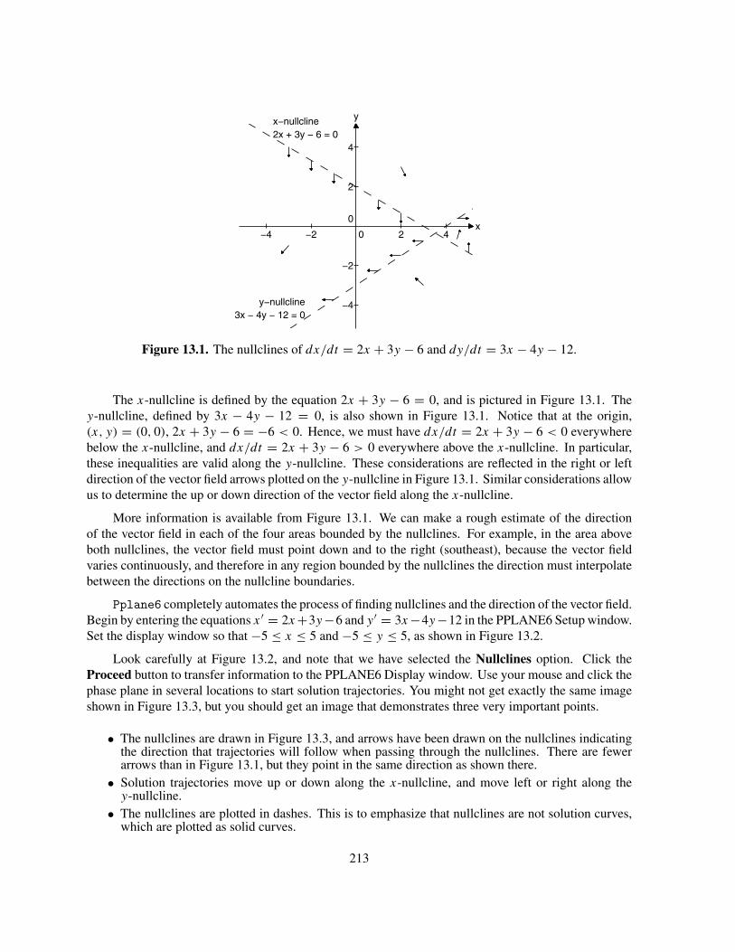
2x + 3y − 6 = 0x−nullcline

3x − 4y − 12 = 0y−nullcline

−4 −2 0 2 4

−4

−2

0

2

4

x

y

Figure 13.1. The nullclines of dx/dt = 2x + 3y − 6 and dy/dt = 3x − 4y − 12.

The x-nullcline is defined by the equation 2x + 3y − 6 = 0, and is pictured in Figure 13.1. They-nullcline, defined by 3x − 4y − 12 = 0, is also shown in Figure 13.1. Notice that at the origin,(x, y) = (0, 0), 2x + 3y − 6 = −6 < 0. Hence, we must have dx/dt = 2x + 3y − 6 < 0 everywherebelow the x-nullcline, and dx/dt = 2x + 3y − 6 > 0 everywhere above the x-nullcline. In particular,these inequalities are valid along the y-nullcline. These considerations are reflected in the right or leftdirection of the vector field arrows plotted on the y-nullcline in Figure 13.1. Similar considerations allowus to determine the up or down direction of the vector field along the x-nullcline.

More information is available from Figure 13.1. We can make a rough estimate of the directionof the vector field in each of the four areas bounded by the nullclines. For example, in the area aboveboth nullclines, the vector field must point down and to the right (southeast), because the vector fieldvaries continuously, and therefore in any region bounded by the nullclines the direction must interpolatebetween the directions on the nullcline boundaries.

Pplane6 completely automates the process of finding nullclines and the direction of the vector field.Begin by entering the equations x′ = 2x+3y−6 and y′ = 3x−4y−12 in the PPLANE6 Setup window.Set the display window so that −5 ≤ x ≤ 5 and −5 ≤ y ≤ 5, as shown in Figure 13.2.

Look carefully at Figure 13.2, and note that we have selected the Nullclines option. Click theProceed button to transfer information to the PPLANE6 Display window. Use your mouse and click thephase plane in several locations to start solution trajectories. You might not get exactly the same imageshown in Figure 13.3, but you should get an image that demonstrates three very important points.

• The nullclines are drawn in Figure 13.3, and arrows have been drawn on the nullclines indicatingthe direction that trajectories will follow when passing through the nullclines. There are fewerarrows than in Figure 13.1, but they point in the same direction as shown there.

• Solution trajectories move up or down along the x-nullcline, and move left or right along they-nullcline.

• The nullclines are plotted in dashes. This is to emphasize that nullclines are not solution curves,which are plotted as solid curves.

213

Figure 13.2. Setting up x′ = 2x + 3y − 6 and y′ = 3x − 4y − 12.

−5 −4 −3 −2 −1 0 1 2 3 4 5

−5

−4

−3

−2

−1

0

1

2

3

4

5

x

y

x ’ = 2 x + 3 y − 6 y ’ = 3 x − 4 y − 12

−5 −4 −3 −2 −1 0 1 2 3 4 5

−5

−4

−3

−2

−1

0

1

2

3

4

5

x

y

x ’ = 2 x + 3 y − 6 y ’ = 3 x − 4 y − 12

Figure 13.3. The nullclines in thePPLANE6 Display window

Figure 13.4. A second view of the null-clines.

There is another way to display nullclines using pplane6. Return to the Setup window, select theArrows option, and then click Proceed. This will remove the nullclines from the Display window andadd the vector field. Next select Solutions→Show nullclines , in the Display window and the nullclineswill be plotted on top of the vector field as shown in Figure 13.4. You might find this view more revealing,if more cluttered.

Equilibrium Points

Consider again the planar, autonomous system

x′ = f (x, y),

y′ = g(x, y).

214

A point (x, y) in the phase plane is called an equilibrium point if both right-hand sides vanish, i.e., iff (x, y) = 0 and g(x, y) = 0. This means that equilibrium points are the points of intersection of thenullclines.

Example 2. Find all equilibrium points of the system in Example 1.

Setting both of the right-hand sides in (13.3) equal to zero yields the system

2x + 3y = 6,

3x − 4y = 12.

This linear system is easily solved, either by hand or using MATLAB, to find that x = 60/17 ≈ 3.5294and y = −6/17 ≈ −0.3529.

Pplane6 can also be used to find equilibrium points. Re-enter the system of Example 1 in thePPLANE6 Setup window as shown in Figure 13.2. Select the Nullclines for the direction field, clickProceed, then start a few trajectories by clicking the mouse in the phase plane. Select Solutions→Findan equilibrium point, then move the mouse “cross hairs” near the intersection of the nullclines and clickthe mouse. Pplane6 will plot the equilibrium point, as shown in Figure 13.5.

−5 −4 −3 −2 −1 0 1 2 3 4 5

−5

−4

−3

−2

−1

0

1

2

3

4

5

x

y

x ’ = 2 x + 3 y − 6 y ’ = 3 x − 4 y − 12

Figure 13.5. The equilibrium point in Example 2 is the intersection point of the nullclines.

Pplane6 also opens the PPLANE6 Equilibrium point data window, which summarizes a num-ber of important facts about the equilibrium point. The first entry says “There is a saddle point at(3.5294, −0.35294).” The location agrees with what we found earlier. The equilibrium point is called asaddle point because, if you have a topographic map of an area including a mountain pass or a saddle,the topographic lines of equal altitude look something like the solution curves in Figure 13.5. Click theGo Away button to close the window.

Example 3. Find all equilibrium points of the system

x′ = x2 + y2 − 4,

y′ = x − y2.(13.4)

215

Setting the right-hand sides of the differential equations in (13.4) equal to zero, we obtain the system

x2 + y2 − 4 = 0,

x − y2 = 0.

This system is nonlinear, but it can be solved by substituting y2 = x in the first equation, and solvingthe resulting quadratic equation, finding x = (−1 ± √

17)/2. For each solution there are two possiblevalues of y satisfying y2 = x. Since one of the values of x is negative, the only viable solutions are

(

−1 + √17

2,

√

−2 + 2√

17

2

)

≈ (1.5616, 1.2496), and

(

−1 + √17

2, −√

−2 + 2√

17

2

)

≈ (1.5616, −1.2496).

(13.5)

Symbolic Toolbox Users. Owners of the Symbolic Toolbox can use the solve command to find theequilibrium points.

>> [x,y]=solve('x^2+y^2-4=0','x-y^2=0','x,y')x =[ -1/2+1/2*17^(1/2)][ -1/2+1/2*17^(1/2)][ -1/2-1/2*17^(1/2)][ -1/2-1/2*17^(1/2)]y =[ 1/2*(-2+2*17^(1/2))^(1/2)][ -1/2*(-2+2*17^(1/2))^(1/2)][ 1/2*(-2-2*17^(1/2))^(1/2)][ -1/2*(-2-2*17^(1/2))^(1/2)]

The first two entries of vectors x and y contain symbolic results identical to our algebraic results in (13.5).To find the numerical values, change the class of x and y to double.

>> S=[double(x),double(y)]S =

1.5616 1.24961.5616 -1.2496

-2.5616 0 + 1.6005i-2.5616 0 - 1.6005i

The first two rows of S contain the equilibrium points; the last two rows of S are complex, and are ignored.

Of course, pplane6 should provide identical results. Enter the system in (13.4) into the PPLANE6Setup window. Set the display window so that −5 ≤ x ≤ 5 and −5 ≤ y ≤ 5. Select Nullclines for thedirection field, then click Proceed to transfer information to the PPLANE6 Display window. Notice thatthe x-nullcline is a circle, and the y-nullcline is a parabola. They have two points of intersection. These

216

are the equilibrium points and they can be found using Solutions→Find an equilibrium point. Clickthe mouse in the phase plane to start several solution trajectories near each equilibrium point, similar tothe image shown in Figure 13.6.

Notice that solutions near the upper of the two equilibrium points behave like those near the saddlepoint in Example 2, while the solution curves near the lower equilibrium point behave quite differently.Select Solutions→Find an equilibrium point and click the mouse near the upper equilibrium point.Repeat the process with the lower equilibrium point. This will open the PPLANE6 Equilibrium pointdata window shown in Figure 13.7. This window indicates that the lower equilibrium point is located atapproximately (1.5616, −1.2496), in agreement with (13.5). Since the solution trajectories in Figure 13.6spiral away from the lower equilibrium point, it is called a spiral source.

−5 −4 −3 −2 −1 0 1 2 3 4 5

−5

−4

−3

−2

−1

0

1

2

3

4

5

x

y

x ’ = x2 + y2 − 4y ’ = x − y2

Figure 13.6. The two equilibrium points inExample 3 are a saddle point and a source.

Figure 13.7. Description of the lower equi-librium point.

Linear Systems

The systemx′ = ax + by,

y′ = cx + dy,(13.6)

is planar, autonomous, and linear. The system can be written in the form

x′ =[

x

y

]′=[

a b

c d

] [

x

y

]

= Ax.

The equilibrium points are found by setting the right-hand sides of both differential equations in (13.6)equal to zero, leading to the system

ax + by = 0,

cx + dy = 0,or Ax = 0. (13.7)

Thus, the equilibrium points are the vectors in the nullspace of the coefficient matrix A. If det A �= 0,the system in (13.7) has a unique solution, so the origin (x, y) = (0, 0) is the only equilibrium point of

217

the system in (13.6). On the other hand, if det A = 0, then the system has many equilibrium points. Forexample, the system x′ = x + 2y, y′ = 2x + 4y has an entire line of equilibrium points. Experimentwith this system in pplane6.

Example 4. Find and classify the equilibrium point of the linear system

x′ = −2x − 2y,

y′ = 3x + y.(13.8)

Select Gallery→linear system from the PPLANE6 Setup menu. Notice that most of the work hasbeen done for you. All you have to do is adjust the parameters A, B, C, and D. Compare system (13.8)with the general linear system (13.6) and note that a = −2, b = −2, c = 3, and d = 1. Enter theseparameters for A, B, C, and D in the PPLANE6 Setup window, then click Proceed to transfer informationto the PPLANE6 Display window. Select Solutions→Keyboard input and start a solution trajectorywith initial condition (0, 1). Note how this solution trajectory “spirals inward” toward the origin, asshown in Figure 13.8.

−5 −4 −3 −2 −1 0 1 2 3 4 5

−5

−4

−3

−2

−1

0

1

2

3

4

5

x

y

x ’ = A x + B yy ’ = C x + D y

B = − 2D = 1

A = − 2C = 3

Figure 13.8. A spiral sink at the equilib-rium point (0, 0).

Figure 13.9. Description of the equilib-rium point in Figure 13.8.

Select Solutions→Find an equilibrium point and click your mouse near the origin in the phaseplane. Let’s carefully examine the information provided in the PPLANE6 Equilibrium point data windowshown in Figure 13.9.

• The first entry provides the type of the equilibrium point and the location, in this case a spiral sinkat (0,0). This certainly agrees with our view of the trajectory in Figure 13.8.

• Next we are presented with the the Jacobian matrix,

J =[−2 −2

3 1

]

218

in this case. If system (13.8) is written in matrix form x′ = Ax, then the Jacobian J is identical tothe coefficient matrix A. This is always the case for linear systems.

• The eigenvalue-eigenvector pairs of the Jacobian are reported. In this case the eigenvalues are acomplex conjugate pair and the eigenvectors are also complex.

• Finally, there is a Display the linearization button. This will provide no new information in thiscase, since system in (13.8) is already linear.

Nonlinear Systems

Any planar, autonomous system that is not in the precise form of (13.6) is nonlinear. Nonlinearsystems are much harder to analyze than linear systems since they rarely possess analytical solutions.Therefore, we must use qualitative analysis and numerical solutions. There are many techniques foranalyzing nonlinear systems qualitatively. One of the most useful is the analysis of the behavior ofsolutions near equilibrium points using the linearization.

If the term linearization sounds familiar, it should. In your first calculus class, you constantlyanalyzed the behavior of a function at a point by approximating the function with a first order Taylor’sseries, whose graph is the line through the point on the graph with the same slope as the graph. This lineis called the tangent line, and its slope is equal to the derivative of the function. The graph of the tangentline closely approximates that of the function near the point of tangency, but as you move away fromthe point of tangency, the approximation is less accurate. Therefore the technique of linearization onlyprovides local information about the behavior of the function.

We will use the same technique to analyze a nonlinear system near an equilibrium point. We willuse the first order Taylor series approximation of the right-hand side of the system. The analog ofthe derivative is called the Jacobian. For some systems, the linearization will enable us to predict thebehavior of solutions near the equilibrium point. Again, as we move away from the equilibrium point,the approximation deteriorates, so the information is only of value locally, by which we mean near theequilibrium point.

Definition. Suppose that a planar vector field is defined by

F(x, y) =[

f (x, y)

g(x, y)

]

.

Then the Jacobian of F is defined to be

JF(x, y) =[

fx(x, y) fy(x, y)

gx(x, y) gy(x, y)

]

,

where fx(x, y) denotes the partial derivative of f with respect to x, evaluated at (x, y), etc.

Example 5. Consider the nonlinear system of differential equations

x′ = 4x − 2x2 − xy,

y′ = y − y2 + 2xy.(13.9)

Find the Jacobian of the vector field.

219

The right-hand side of the system in (13.9) can be written as the vector field

F(x, y) =[

f (x, y)

g(x, y)

]

=[

4x − 2x2 − xy

y − y2 + 2xy

]

.

The Jacobian matrix of F is

JF(x, y) =[

fx(x, y) fy(x, y)

gx(x, y) gy(x, y)

]

=[

4 − 4x − y −x

2y 1 − 2y + 2x

]

. (13.10)

Symbolic Toolbox Users. The Symbolic Toolbox can compute the Jacobian.

>> syms x y>> F=[4*x-2*x^2-x*y;y-y^2+2*x*y]F =[ 4*x-2*x^2-x*y][ y-y^2+2*x*y]>> JF=jacobian(F)JF =[ 4-4*x-y, -x][ 2*y, 1-2*y+2*x]

You can also use the command subs to evaluate the Jacobian at a particular point.

>> subs(JF,{x,y},{3/4,5/2})ans =

-1.5000 -0.75005.0000 -2.5000

Consequently,

JF(3/4, 5/2) =[−1.5 −0.75

5 −2.5

]

. (13.11)

Pplane6 can greatly simplify the analysis of nonlinear systems.

Example 6. The system

x′ = 2x(2 − x) − xy,

y′ = y(1 − y) + 2xy.(13.12)

models the interaction of two populations, a rabbit population x and a fox population y. Find and analyzethe equilibrium points of this system.

220

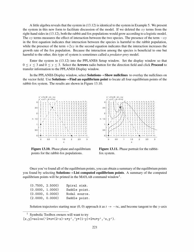
A little algebra reveals that the system in (13.12) is identical to the system in Example 5. We presentthe system in this new form to facilitate discussion of the model. If we deleted the xy terms from theright-hand sides in (13.12), both the rabbit and fox populations would grow according to a logistic model.The xy terms measures the effect of interaction between the two species. The presence of the term −xy

in the first equation indicates that interaction between the species is harmful to the rabbit population,while the presence of the term +2xy in the second equation indicates that the interaction increases thegrowth rate of the fox population. Because the interaction among the species is beneficial to one butharmful to the other, this type of system is sometimes called a predator-prey model.

Enter the system in (13.12) into the PPLANE6 Setup window. Set the display window so that0 ≤ x ≤ 3 and 0 ≤ y ≤ 3. Select the Arrows radio button for the direction field and click Proceed totransfer information to the PPLANE6 Display window.

In the PPLANE6 Display window, select Solutions→Show nullclines to overlay the nullclines onthe vector field. Use Solutions→Find an equilibrium point to locate all four equilibrium points of therabbit-fox system. The results are shown in Figure 13.10.

0 0.5 1 1.5 2 2.5 3

0

0.5

1

1.5

2

2.5

3

x

y

x ’ = 2 x (2 − x) − x yy ’ = y (1 − y) + 2 x y

0 0.5 1 1.5 2 2.5 3

0

0.5

1

1.5

2

2.5

3

x

y

x ’ = 2 x (2 − x) − x yy ’ = y (1 − y) + 2 x y

Figure 13.10. Phase plane and equilibriumpoints for the rabbit-fox populations.

Figure 13.11. Phase portrait for the rabbit-fox system.

Once you’ve found all of the equilibrium points, you can obtain a summary of the equilibrium pointsyou found by selecting Solutions→List computed equilibrium points. A summary of the computedequilibrium points will be printed in the MATLAB command window1.

(0.7500, 2.5000) Spiral sink.(0.0000, 1.0000) Saddle point.(0.0000, 0.0000) Nodal source.(2.0000, 0.0000) Saddle point.

Solution trajectories starting near (0, 0) approach it as t → −∞, and become tangent to the y-axis

1 Symbolic Toolbox owners will want to try[x,y]=solve(’2*x*(2-x)-x*y’,’y*(1-y)+2*x*y’,’x,y’).

221

in the process. An equilibrium point with the property that all solutions starting nearby tend towards itas t → −∞, and become tangent to a fixed direction is called a “nodal source.”

The points (0, 1) and (2, 0) are saddle points. Click your mouse near these points and note thatsolutions tend toward these points, only to veer away at the last moment.

Finally, the equilibrium point at (0.75, 2.5) is called a spiral sink. Think of the drain in a bathtub,with water swirling around and into the drain. Click your mouse near the point (0.75, 2.5) to witnessthis behavior.

If you’ve carefully followed the directions in the preceding paragraphs, Figure 13.11 shows a possiblephase portrait for the rabbit-fox system.

Linearization. Let revisit the spiral sink at (0.75, 2.5). Select Solutions→Find an equilibrium pointand click near the point (0.75, 2.5) to re-open the PPLANE6 Equilibrium point data window, shown inFigure 13.12.

Figure 13.12. Data for the spiral sink at (0.75, 2.5).

The first line in the PPLANE6 Equilibrium point data window indicates that there is a spiral sinkat (0.75, 2.5). The Jacobian matrix evaluated at the equilibrium point (0.75, 2.5), and its eigenvalue-eigenvector pairs are displayed. Click the Display the linearization button to show the linear approxi-mation of the rabbit-fox system shown in Figure 13.13.

The title heading in Figure 13.13 holds the key to the relationship between the Jacobian and thelinearization. Notice that the system in Figure 13.13 is the general linear system

u′ = Au + Bv

v′ = Cu + Dv

The coefficients are given to the right of the system. Notice that the values of A, B, C, and D are preciselythe entries in the Jacobian matrix reported in the PPLANE6 Equilibrium point data window shown inFigure 13.12. So, you’ve now got the secret! If you want a linearization of a nonlinear system at anequilibrium point, compute the Jacobian at the equilibrium point, and form a linear system using theentries of the Jacobian matrix.

Actually, we are hiding a little mathematics here. Note that the linearization in Figure 13.13 hasan equilibrium point at (0, 0), while the equilibrium point for the nonlinear system in (13.11) is at(0.75, 2.5). When forming the linearization, we have to translate coordinate systems so that the origin

222

−1 −0.5 0 0.5 1

−1

−0.8

−0.6

−0.4

−0.2

0

0.2

0.4

0.6

0.8

1

u

v

u’ = A u + B vv’ = C u + D v

B = −0.75D = −2.5

A = −1.5C = 5

0 0.5 1 1.5

2

2.1

2.2

2.3

2.4

2.5

2.6

2.7

2.8

2.9

3

x

y

x ’ = 2 x (2 − x) − x yy ’ = y (1 − y) + 2 x y

Figure 13.13. The linearization of the sys-tem at (0.75, 2.5).

Figure 13.14. A closer look at the equilib-rium point at (0.75, 2.5).

of the linearization aligns itself with the equilibrium point (0.75, 2.5). That’s why we’re using u and v

coordinates to define the linearization. They are the coordinates of the translated coordinate system.

Zoom in square. If we compare the solutions of the linearization in Figure 13.13 to those of the nonlinearsystem in Figure 13.11, we see that there are many differences, although the solutions to the nonlinearsystem near the equilibrium point at (0.75, 2.5) do resemble those of the linearization near the origin. Ifwe remember that the linearization provides a good approximation only near the equilibrium point, wecan understand that.

If we want to compare the nonlinear system and its linearization, we should zoom in near theequilibrium point for the nonlinear system. Notice that the linearization window in Figure 13.13 issquare, and that both variables range from −1 to 1. In other words, the scales are the same on eachaxis. When you zoom in in the usual way using Edit→Zoom in in the PPLANE6 Display window, it ishighly unlikely that the scales will be the same on the two axes. However, if you choose Edit→Zoomin square, you automatically get a new window with the same scale on the two axes. After making themenu selection, click the (left) mouse button on the equilibrium point is the Display window and drag asmall rectangle.2

One possible result of this process for the system in Figure 13.11 is shown in Figure 13.14. Noticethat the solution curves for the linearization in Figure 13.13 and those for the nonlinear system inFigure 13.14 are very similar. These two figures also clearly display the fact that the equilibrium pointsfor the nonlinear system and its linearization are different. Obtaining the similarity we observe betweenFigures 13.13 and 13.14 may require several zooms. For some systems the attempt to achieve similarityis doomed to failure. (See Exercise 20.)

2 If you have a three button mouse, you do not need to use the menu. Simply click and drag with thecenter button.

223

Classification of equilibrium points. It turns out that there is a small list of all possible equilibriumpoints for planar, linear systems with constant coefficients. We have seen saddle points, nodal sources,nodal sinks, spiral sources, and spiral sinks. Another is a center, which is an equilibrium point surroundedby closed solution curves.3 The behavior of the solutions is completely determined by the eigenvaluesand eigenvectors of the coefficient matrix.

For nonlinear systems there are more possibilities, but in many cases the type of an equilibriumpoint is the same as that of the linearization at that point. We see this clearly for the equilibrium pointstudied in Figures 13.13 and 13.14. When you find an equilibrium point using pplane6, the PPLANE6Equilibrium point window gives as much information about the equilibrium point as it can, based on itsanalysis of the linearization. In some cases it gives all the information you need. In others you will beable to find more precise information by further analysis of the system. We will offer some examplesin the exercises. In the Appendix to this chapter you will find a complete list of the messages that canappear in the PPLANE6 Equilibrium point window, together with an interpretation of what each messagemeans.

Separatrices

There are four special solution curves associated with any saddle point. There are two curves thatapproach the saddle point at t → ∞, called stable solution curves, and two that approach the saddlepoint at t → −∞, called unstable solution curves. Collectively, these curves are called separatrices.4

This is best demonstrated with an example.

Example 7. Consider the nonlinear system

x′ = x(2 − x) − 2xy,

y′ = y(2 − y) − 2xy.(13.13)

Assume that x and y represent populations that are always non-negative.

Without the xy terms, the equation for each population would be the logistic equation. However,because of the minus signs, including the xy terms in this model is detrimental to the growth of bothpopulations. This is an example of competition. Think about sheep and cattle populations competing forthe same grazing land.

Enter the system into the PPLANE6 Setup window, set the display window to 0 ≤ x ≤ 3 and0 ≤ y ≤ 3, select Arrows for the direction field, and click Proceed to transfer information to thePPLANE6 Display window.

In the PPLANE6 Display window, select Solutions→Show nullclines to overlay the nullclines onthe direction field. Use Solutions→Find an equilibrium point to find the four equilibrium points. Se-lecting Solutions→List computed equilibrium points will show the following summary in MATLAB’scommand window.

(0.0000, 2.0000) Sink.(0.0000, 0.0000) Source.(2.0000, 0.0000) Sink.(0.6667, 0.6667) Saddle point.

3 There are a number of others that appear less frequently.4 The singular is separatrix.

224

Compute some solution trajectories by clicking various initial conditions in the phase plane. You willsoon discover that some of the solutions tend to the sink at (0, 2), spelling extinction for species x, whileother trajectories tend to the sink at (2, 0), indicating extinction of species y.

Select Solutions→Plot stable and unstable orbits and click near the saddle point at (0.6667,

0.6667). Pplane6 will plot the separatrices in green. Notice that the stable solution curves “separate”solution trajectories that tend to the sink at (0, 2) from those that tend to the sink at (2, 0), as shown inFigure 13.15.

0 0.5 1 1.5 2 2.5 3

0

0.5

1

1.5

2

2.5

3

x

yx ’ = x (2 − x) − 2 x yy ’ = y (2 − y) − 2 x y

Figure 13.15. The separatrices divide the phase plane into basins of attraction.

For any sink there is a basin of attraction, consisting of the initial points of solutions which tend tothe sink as t → ∞. We see in Figure 13.15 that the stable trajectories form the boundary of the basinsof attraction of the two sinks. Separatrices often separate the phase plane into areas where the solutioncurves behave differently. This explains the special importance of separatrices as well as their name.

Limit Sets of Solution Curves

Perhaps you have noticed that you do not have to provide a solution interval for a solution computedby pplane6, although it is necessary to do so when solving using ode45 and any other solver. Perhaps youhave wondered how pplane6 knows when to stop computing. You may also have noticed the messagesthat appear in the message window, telling you that a solution ... left the computation window,or ...--> a possible eq. pt. near .... These messages actually reveal how pplane6 knowswhen to stop. It turns out that there is a very small list of the possible “endings” of a solution curve.

What you see in the PPLANE6 Display window is only a fraction of what’s being computed. Thereis a computation window that’s larger than what is actually displayed and allows solutions to leave theDisplay window and return. One possible ending of a computed solution is that it escapes this computationwindow. If it does, pplane6 stops computing. The interesting story is about what can happen to a solutionthat stays in the computation window forever.

What we referred to as the “ending” of a solution curve is officially called the limit set of the curve.

225

At the beginning of the twentieth century, the mathematicians Henri Poincaré and Ivar Bendixson provedthat there are only three possible limit sets for a solution curve that stays in a bounded region:

• An equilibrium point.• A closed solution curve.• A directed planar graph with vertices that are equilibrium points and edges that are solution curves.

These are called the Poincaré-Bendixson alternatives. We have seen many examples of the first alternative.In each case this result was reported in the message window.

A closed solution curve can occur as the limit set in two ways. First of all, the solution curve itselfcan be closed. Examples of this can be found with any center. In particular, choose vibrating springfrom the Gallery menu, and leave the damping term d = 0. Plot a few solutions. See Figure 13.16. Theother possibility is that the solution curve is not closed, but approaches a closed curve that is called a limitcycle. Choose van der Pol’s equation from the Gallery menu for an example, and plot a few solutions.See Figure 13.17. A closed solution curve repeats itself, while a solution curve which spirals toward alimit cycle, gets closer to itself in the process. pplane6 has a way of discovering when a solution curvegets very close to itself. It stops the computation when this occurs and reports in the message windowthat the solution curve ... --> a nearly closed orbit. The word “nearly” is there to allow forthe possibility that pplane6 is making a mistake, but our experience has been that this is a rare event.Most of the time this message means that the solution curve is either closed itself or is approaching alimit cycle.

−5 −4 −3 −2 −1 0 1 2 3 4 5

−5

−4

−3

−2

−1

0

1

2

3

4

5

x

v

x ’ = v v ’ = − (k x + d v)/m

m = 1d = 0

k = 3

−5 −4 −3 −2 −1 0 1 2 3 4 5

−5

−4

−3

−2

−1

0

1

2

3

4

5

x

y

x ’ = M x − y − x3

y ’ = x M = 2

Figure 13.16. Closed orbits around a cen-ter.

Figure 13.17. Orbits approaching a limitcycle.

If you want to plot only the “nearly closed curve,” select Solutions→Find a nearly closed orbit,and select the direction along the solution curve in which to search. The result is reported in the messagewindow. If such a curve is found, it is plotted in the display window and its period is reported in themessage window. This feature is especially useful if you want to see what a limit cycle actually lookslike. Approximately three periods of the closed curve will be plotted. See Figure 13.18.

An example of the third Poincaré-Bendixson alternative can be seen by selecting square limit setfrom the gallery. If you start a solution anywhere inside the unit square, the solution will spiral out to theboundary of the unit square, so this boundary is the limit set. Verify that the vertices of the unit squareare saddle points, and the edges are separatrices. Since separatrices are solution curves, the limit set is

226

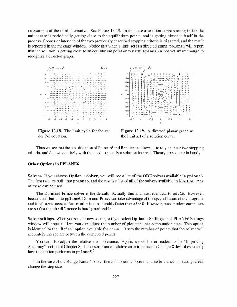
an example of the third alternative. See Figure 13.19. In this case a solution curve starting inside theunit square is periodically getting close to the equilibrium points, and is getting closer to itself in theprocess. Sooner or later one of the two previously described stopping criteria is triggered, and the resultis reported in the message window. Notice that when a limit set is a directed graph, pplane6 will reportthat the solution is getting close to an equilibrium point or to itself. Pplane6 is not yet smart enough torecognize a directed graph.

−5 −4 −3 −2 −1 0 1 2 3 4 5

−5

−4

−3

−2

−1

0

1

2

3

4

5

x

y

x ’ = M x − y − x3

y ’ = x M = 2

−1.5 −1 −0.5 0 0.5 1 1.5

−1

−0.8

−0.6

−0.4

−0.2

0

0.2

0.4

0.6

0.8

1

xy

x ’ = (y + x/5) (1 − x2)y ’ = − x (1 − y2)

Figure 13.18. The limit cycle for the vander Pol equation.

Figure 13.19. A directed planar graph asthe limit set of a solution curve.

Thus we see that the classification of Poincaré and Bendixson allows us to rely on these two stoppingcriteria, and do away entirely with the need to specify a solution interval. Theory does come in handy.

Other Options in PPLANE6

Solvers. If you choose Option→Solver, you will see a list of the ODE solvers available in pplane6.The first two are built into pplane6, and the rest is a list of all of the solvers available in MATLAB. Anyof these can be used.

The Dormand-Prince solver is the default. Actually this is almost identical to ode45. However,because it is built into pplane6, Dormand-Prince can take advantage of the special nature of the program,and it is faster to access. As a result it is considerably faster thanode45. However, most modern computersare so fast that the difference is hardly noticeable.

Solver settings. When you select a new solver, or if you select Option→Settings, the PPLANE6 Settingswindow will appear. Here you can adjust the number of plot steps per computation step. This optionis identical to the “Refine” option available for ode45. It sets the number of points that the solver willaccurately interpolate between the computed points.

You can also adjust the relative error tolerance. Again, we will refer readers to the “ImprovingAccuracy” section of Chapter 8. The description of relative error tolerance in Chapter 8 describes exactlyhow this option performs in pplane6.5

5 In the case of the Runge-Kutta 4 solver there is no refine option, and no tolerance. Instead you canchange the step size.

227

In the second part of the PPLANE6 Settings window, there is a slider that will enable you to choosethe speed with which solutions are computed and plotted. This is meant to be used to slow down thesolution to allow you to better understand how the solution proceeds. Choose less than 10 steps persecond for a full appreciation of this option.

Finally, there is a setting for determining the size of the calculation window. The default settingof 3.5 is sufficient for ordinary use of pplane6, but if you notice that some solutions which leave thedisplay window do not return although you know they should, increase this parameter.

Conservative and dissipative systems and level curves. The selection Solutions→Plot level curveswill open the PPLANE6 Level sets window, which will enable you to plot the level curves of a functionin the Display window. As an example, select pendulum from the gallery. The total energy for thependulum is (proportional to) E(θ, ω) = ω2/2 − cos θ. If you leave D = 0, Proceed to the displaywindow, and select Solutions→Plot level curves, you will be presented with the window shown inFigure 13.16.

Figure 13.20. Entering the energy for the pendulum.

Notice that the first line says the function should be entered in terms of omega and theta, not interms of the TEX notation \omega and \theta used in the setup window. Enter the rest of the data shownin Figure 13.16, and click Proceed. The sets of constant energy will be plotted. Now compute a fewsolutions and notice that the solution curves are identical to the level curves, demonstrating that energyis conserved in the motion of the undamped pendulum.

Return to the setup window, increase the damping constant to D = 0.5, and repeat the process. Thistime the solution curves consistently move from higher to lower energy levels, showing that dampingdissipates the energy of the system.

Marking initial points. Sometimes it is advantageous to mark the initial points of the computed solutions.Choosing Option→Mark initial points will enable you to do just that.

Exporting solution data. If you have computed a solution curve that you want to analyze using techniquesnot available in pplane6, you can export the data to the MATLAB command window. Select Option→Export solution data. If there is only one solution curve, its data will be exported. If there are morethan one, you will be given the opportunity to choose which one to export with the mouse. The actionis reported in the message window with a message like, The data has been exported as thestructure ppdata4 with fields t, x, and y. A structure is a MATLAB class that is convenient

228

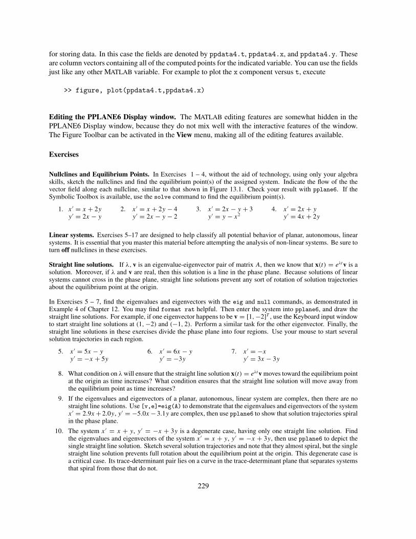
for storing data. In this case the fields are denoted by ppdata4.t, ppdata4.x, and ppdata4.y. Theseare column vectors containing all of the computed points for the indicated variable. You can use the fieldsjust like any other MATLAB variable. For example to plot the x component versus t, execute

>> figure, plot(ppdata4.t,ppdata4.x)

Editing the PPLANE6 Display window. The MATLAB editing features are somewhat hidden in thePPLANE6 Display window, because they do not mix well with the interactive features of the window.The Figure Toolbar can be activated in the View menu, making all of the editing features available.

Exercises

Nullclines and Equilibrium Points. In Exercises 1 – 4, without the aid of technology, using only your algebraskills, sketch the nullclines and find the equilibrium point(s) of the assigned system. Indicate the flow of the thevector field along each nullcline, similar to that shown in Figure 13.1. Check your result with pplane6. If theSymbolic Toolbox is available, use the solve command to find the equilibrium point(s).

1. x ′ = x + 2yy ′ = 2x − y

2. x ′ = x + 2y − 4y ′ = 2x − y − 2

3. x ′ = 2x − y + 3y ′ = y − x2

4. x ′ = 2x + yy ′ = 4x + 2y

Linear systems. Exercises 5–17 are designed to help classify all potential behavior of planar, autonomous, linearsystems. It is essential that you master this material before attempting the analysis of non-linear systems. Be sure toturn off nullclines in these exercises.

Straight line solutions. If λ, v is an eigenvalue-eigenvector pair of matrix A, then we know that x(t) = eλtv is asolution. Moreover, if λ and v are real, then this solution is a line in the phase plane. Because solutions of linearsystems cannot cross in the phase plane, straight line solutions prevent any sort of rotation of solution trajectoriesabout the equilibrium point at the origin.

In Exercises 5 – 7, find the eigenvalues and eigenvectors with the eig and null commands, as demonstrated inExample 4 of Chapter 12. You may find format rat helpful. Then enter the system into pplane6, and draw thestraight line solutions. For example, if one eigenvector happens to be v = [1, −2]T , use the Keyboard input windowto start straight line solutions at (1, −2) and (−1, 2). Perform a similar task for the other eigenvector. Finally, thestraight line solutions in these exercises divide the phase plane into four regions. Use your mouse to start severalsolution trajectories in each region.

5. x ′ = 5x − yy ′ = −x + 5y

6. x ′ = 6x − yy ′ = −3y

7. x ′ = −xy ′ = 3x − 3y

8. What condition on λ will ensure that the straight line solution x(t) = eλtv moves toward the equilibrium pointat the origin as time increases? What condition ensures that the straight line solution will move away fromthe equilibrium point as time increases?

9. If the eigenvalues and eigenvectors of a planar, autonomous, linear system are complex, then there are nostraight line solutions. Use [v,e]=eig(A) to demonstrate that the eigenvalues and eigenvectors of the systemx ′ = 2.9x + 2.0y, y ′ = −5.0x − 3.1y are complex, then use pplane6 to show that solution trajectories spiralin the phase plane.

10. The system x ′ = x + y, y ′ = −x + 3y is a degenerate case, having only one straight line solution. Findthe eigenvalues and eigenvectors of the system x ′ = x + y, y ′ = −x + 3y, then use pplane6 to depict thesingle straight line solution. Sketch several solution trajectories and note that they almost spiral, but the singlestraight line solution prevents full rotation about the equilibrium point at the origin. This degenerate case isa critical case. Its trace-determinant pair lies on a curve in the trace-determinant plane that separates systemsthat spiral from those that do not.

229

Sources, sinks, and saddles. If a system has two distinct, real eigenvalues, then it will have two independentstraight line solutions, and all solutions can be written as a linear combination of these two straight line solutions, asin x(t) = c1e

λ1tv1 + c2eλ2 tv2.

11. Nodal sink. If a system has two distinct negative eigenvalues, then both straight line solutions will decay tothe origin with the passage of time. Consequently, all solutions will decay to the origin. Enter the system,x ′ = −4x +y, y ′ = −2x −y, in pplane6 and plot the straight line solutions. Plot several more solutions andnote that they also decay to the origin. Select Solutions→Find an equilibrium point, find the equilibriumpoint at the origin, then read its classification from the PPLANE6 Equilibrium point data window.

12. Nodal source. If a system has two distinct positive eigenvalues, then both straight line solutions will moveaway from the origin with the passage of time. Consequently, all solutions will move away from the origin.Enter the system, x ′ = 5x − y, y ′ = 2x + 2y, in pplane6 and plot the straight line solutions. Plot severalmore solutions and note that they also move away from the origin. Select Solutions→Find an equilibriumpoint, find the equilibrium point at the origin, then read its classification from the PPLANE6 Equilibriumpoint data window.

13. Saddle. If a system has one negative and one positive eigenvalue, then one straight line solution moves towardthe origin and the other moves away. Consequently, general solutions (being linear combinations of straightline solutions) must do the same thing. Enter the system x ′ = 9x − 14y, y ′ = 7x − 12y, in pplane6 andplot the straight line solutions. Plot several more solutions and note that they move toward the origin only tomove away at the last moment. Select Solutions→Find an equilibrium point, find the equilibrium point atthe origin, then read its classification from the PPLANE6 Equilibrium point data window.

Spiral sources, spiral sinks, and centers. If the eigenvalues are complex, then a planar, autonomous, linear systemhas no straight line solutions. Consequently, trajectories are free to spiral.

14. Spiral source. As we saw in equation (13.12), if the real part of a complex eigenvalue is negative, theequilibrium point will be a spiral sink. What happens if the real part of the complex eigenvalue is positive?Enter the system x ′ = 2.1x + 5.0y, y ′ = −1.0x − 1.9y in pplane6 and note that solutions spiral outwardwith the passage of time. Select Solutions→Find an equilibrium point, find the equilibrium point at theorigin, note the real part of the complex eigenvalue, then note the classification of the equilibrium point inthe PPLANE6 Equilibrium point data window. If your computer is too fast to differentiate an outward spiralfrom an inward spiral, you might try Options→Solution direction→Forward.

15. Center. If the real part of the complex eigenvalue is zero, there can be no growth or decay of solutiontrajectories. Enter the system x ′ = −x + y, y ′ = −2x + y, and note that pplane6 reports a nearly closedorbit in its message window. Note that pplane6 has difficulty with this type of equilibrium point, commonlycalled a center. It should report that the trajectories are purely periodic. This happens because this system isa critical case, separating linear systems with a spiral sink from systems with a spiral source. The slightestnumerical error, even an error of 1×10−16, makes the real part of the complex eigenvalue non-zero, indicatinga spiral source or sink.

16. Summarizing your findings. In a table use your results from Exercises 11–15 to list conditions on theeigenvalue that predict when the equilibrium point at the origin is a nodal source, nodal sink, saddle, spiralsource, spiral sink, and center.

17. The trace-determinant plane. It is a nice exercise to classify linear systems based on their position in thetrace-determinant plane. Consider the matrix

A =[

a b

c d

]

.

a) Show that the characteristic polynomial of the matrix A is p(λ) = λ2 − T λ + D, where T = a + dis the trace of A and D = det(A) = ad − bc is the determinant of A.

b) We know that the characteristic polynomial factors as p(λ) = (λ − λ1)(λ − λ2), where λ1 and λ2

are the eigenvalues. Use this and the result of part (a) to show that the product of the eigenvalues isequal to the determinant of matrix A. Note: This is a useful fact. For example, if the determinant isnegative, then you must have one positive and one negative eigenvalue, indicating a saddle equilibriumpoint. Also, show that the sum of the eigenvalues equals the trace of matrix A.

230

c) Show that the eigenvalues of matrix A are given by the formula

λ = T ± √T 2 − 4D

2.

Note that there are three possible scenarios. If T 2 − 4D < 0, then there are two complex eigenvalues.If T 2 − 4D > 0, there are two real eigenvalues. Finally, if T 2 − 4D = 0, then there is one repeatedeigenvalue of algebraic multiplicity two.

d) Draw a pair of axes on a piece of poster board. Label the vertical axis D and the horizontal axisT . Sketch the graph of T 2 − 4D = 0 on your poster board. The axes and the parabola defined byT 2 − 4D = 0 divide the trace-determinant plane into six distinct regions, as shown in Figure 13.17.

D

T

T2 − 4D = 0

Figure 13.21. The trace-determinant plane.

e) You can classify any matrix A by its location in the trace-determinant plane. For example, if

A =[

1 2−3 2

]

,

then T = 3 and D = 8, so the point (T , D) is located in the first quadrant. Furthermore, (3)2 −4(8) <0, placing the point (3, 8) above the parabola T 2 − 4D = 0. Finally, if you substitute T = 3 andD = 8 into the formula λ = (T ± √

T 2 − 4D)/2, then you get eigenvalues that are complex with apositive real part, making the equilibrium point of the system x′ = Ax a spiral source. Use pplane6

to generate a phase portrait of this particular system and attach the printout to the poster board at thepoint (3, 8).

f) Linear systems possess a small number of distinctive phase portraits. Each of these is graphicallydifferent from the others, but each corresponds to the pair of eigenvalues and their multiplicities. Foreach case, use pplane6 to construct a phase portrait, and attach a printout at its appropriate point(T , D) in your poster board trace-determinant plane. Hint: There are degenerate cases on the axesand the parabola. For example, you can find degenerate cases on the parabola in the first quadrant thatseparate nodal sources from spiral sources. There are also a number of interesting degenerate casesat the origin of the trace-determinant plane. One final note: We have intentionally used the words“small number of distinctive cases” so as to spur argument amongst our readers when working on thisactivity. What do you think is the correct number?

Nonlinear Systems. We analyze the behavior of a nonlinear system near an equilibrium point with a linear approx-imation.

231

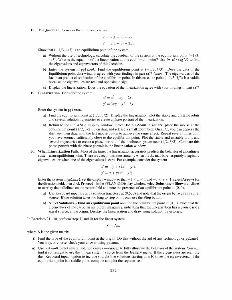
18. The Jacobian. Consider the nonlinear system

x ′ = x(1 − x) − xy,

y ′ = y(2 − y) + 2xy.

Show that (−1/3, 4/3) is an equilibrium point of the system.

a) Without the use of technology, calculate the Jacobian of the system at the equilibrium point (−1/3,4/3). What is the equation of the linearization at this equilibrium point? Use [v,e]=eig(J) to findthe eigenvalues and eigenvectors of this Jacobian.

b) Enter the system in pplane6. Find the equilibrium point at (−1/3, 4/3). Does the data in theEquilibrium point data window agree with your findings in part (a)? Note: The eigenvalues of theJacobian predict classification of the equilibrium point. In this case, the point (−1/3, 4/3) is a saddlebecause the eigenvalues are real and opposite in sign.

c) Display the linearization. Does the equation of the linearization agree with your findings in part (a)?

19. Linearization. Consider the systemx ′ = x2 + xy − 2x,

y ′ = 3xy + y2 − 3y.

Enter the system in pplane6.

a) Find the equilibrium point at (1/2, 3/2). Display the linearization, plot the stable and unstable orbitsand several solution trajectories to create a phase portrait of the linearization.

b) Return to the PPLANE6 Display window. Select Edit→Zoom in square, place the mouse at theequilibrium point (1/2, 3/2), then drag and release a small zoom box. On a PC, you can depress theshift key, then drag with the left mouse button to achieve the same effect. Repeat several times untilyou have zoomed sufficiently close to the equilibrium point. Plot the stable and unstable orbits andseveral trajectories to create a phase portrait of the nonlinear system near (1/2, 3/2). Compare thisphase portrait with the phase portrait in the linearization window.

20. When Linearization Fails. Most of the time, the linearization accurately predicts the behavior of a nonlinearsystem at an equilibrium point. There are exceptions, most notably when the the matrix A has purely imaginaryeigenvalues, or when one of the eigenvalues is zero. For example, consider the system

x ′ = −y + x(x2 + y2),

y ′ = x + y(x2 + y2).

Enter the system in pplane6, set the display window so that −1 ≤ x ≤ 1 and −1 ≤ y ≤ 1, select Arrows forthe direction field, then click Proceed. In the PPLANE6 Display window, select Solutions→Show nullclinesto overlay the nullclines on the vector field and note the presence of an equilibrium point at (0, 0).

a) Use Keyboard input to start a solution trajectory at (0.5, 0) and note that the origin behaves as a spiralsource. If the solution takes too long to stop on its own use the Stop button.

b) Select Solutions→Find an equilibrium point and find the equilibrium point at (0, 0). Note that theeigenvalues of the Jacobian are purely imaginary, indicating that the linearization has a center, not aspiral source, at the origin. Display the linearization and draw some solution trajectories.

In Exercises 21 –30, perform steps i) and ii) for the linear system

x′ = Ax,

where A is the given matrix.

i) Find the type of the equilibrium point at the origin. Do this without the aid of any technology or pplane6.You may, of course, check your answer using pplane.

ii) Use pplane6 to plot several solution curves — enough to fully illustrate the behavior of the system. You willfind it convenient to use the “linear system” choice from the Gallery menu. If the eigenvalues are real, usethe “Keyboard input” option to include straight line solutions starting at ±10 times the eigenvectors. If theequilibrium point is a saddle point, compute and plot the separatrices.

232

21.

[

1 1−18 10

]

22.

[

6 −10 −3

]

23.

[−1 03 −3

]

24.

[

6 1−18 0

]

25.

[

9 −19 3

]

26.

[

9 19 3

]

27.

[

7 4−10 −5

]

28.

[−1 00 −1

]

29.

[

6 −418 −6

]

30.

[

2 −24 −4

]

In Exercises 31 –34 we consider the effect of a non-linear perturbation which leaves the Jacobian at (0, 0) unchanged.The theory predicts that, in (maybe very small) neighborhoods of equilibrium points where the eigenvalues of theJacobian are non-zero and not equal, a non-linear system will act very much like the linear system associated withthe Jacobian. We will use pplane6 to verify this by performing steps i), ii), and iii) below for the system in theindicated exercise.

i) Make up a perturbation for the system that vanishes to second order at the origin. As an example, instead ofthe system in Exercise 21 consider the perturbed system

x ′ = x + y − xy,

y ′ = −18x + 10y − x2 − y2.

ii) Show that the Jacobian of the perturbed system at the origin is the same as that of the unperturbed system.

iii) Starting with the display rectangle −5 ≤ x ≤ 5, −5 ≤ y ≤ 5, zoom in square to smaller squares centered at(0, 0) until the solution curves look like those of the linear system.

31. Exercise 21. 32. Exercise 22. 33. Exercise 23. 34. Exercise 24.

35. In contrast to Exercises 31 – 34, consider the system

x ′ = y + ax3,

y ′ = −x,

for the three values 0, 10 and −10 of the parameter a.

a) Show that all three systems have the same Jacobian matrix at the origin. What type of equilibriumpoint at (0, 0) is predicted by the eigenvalues of the Jacobian?

b) Use pplane6 to find evidence that will enable you to make a conjecture as to the type of the equilibriumpoint at (0, 0) in each of the three cases.

c) Consider the function h(x, y) = x2 + y2. In each of the three cases, restrict h to a solution curve anddifferentiate the result with respect to t (Recall: dh/dt = (∂h/∂x)(dx/dt) + (∂h/∂y)(dy/dt)). Canyou use the result to verify the conjecture you made in part b)? Hint: Note that h(x, y) measures thedistance between the origin and (x, y).

d) Does the Jacobian predict the behavior of the non-linear systems in this case?

36. Consider the systemx ′ = ax + y,

y ′ = −x − 2y.

Describe what happens to the equilibrium points as a varies among the five choices −0.1, −0.01, 0, 0.01,and 0.1. Provide plots of each with enough solution curves to illustrate the behavior of the system. If theeigenvalues are real, use the Keyboard input option to include straight line solutions starting at ±1 timesthe eigenvectors.

37. Consider the damped pendulum when the damping constant is D=0.5 versus when D=2.5.

a) Select Gallery→pendulum and use pplane6 to examine the behavior of the system in each of thesecases.

b) You will notice that the type of the equilibrium point at the origin is different for D=0.5 and D=2.5.Analyze the Jacobian matrix and find out at which value of D the type changes.

233

38. This is another example of how a system can change as a parameter is varied. Consider the system

x ′ = ax + y − x(x2 + y2),

y ′ = −x + ay − y(x2 + y2),

for a = 0, and a = ±0.1. Use the display rectangle −1 ≤ x ≤ 1, and −1 ≤ y ≤ 1, and plot enough solutionsin each case to describe behavior of the system. Describe what happens as the parameter a varies fromnegative values to positive values. (This is an example of a Hopf bifurcation.) Hint: Look for somethingcompletely new, something other than an equilibrium point.

39. This problem involves the default system in pplane6, i.e., the planar system that appears when pplane6 isfirst started.

a) Find and plot all interesting features, i.e., equilibrium points, separatrices, limit cycles, and any otherfeatures that appeal to you. Make a list of such to turn in with the plot.

b) Find the linearization of the system at (0, 0). Enter that into pplane6 and plot a few orbits.

c) Go back to the default system. According to theory, the linearization should approximate the originalsystem in a small enough neighborhood of (0, 0). Use the Zoom in square option to find a smallenough rectangle containing (0, 0), where the behavior of the system is closely approximated by thelinear system you analyzed in part b).

d) Redo parts b) and c) for the other equilibrium points of the default system.

40. Perturbation of the default system in pplane6 exhibits two bifurcations involving the saddle point at the originand the equilibrium point near (3/2, −3/2). To be precise we are looking at the system

x ′ = 2x − y + 3(x2 − y2) + 2xy,

y ′ = x − 3y − 3(x2 − y2) + Axy,

as the parameter A varies.

a) Show that between A = 2.5 and A = 3, the equilibrium point changes from a sink to a source andspawns a limit cycle, i.e., a Hopf bifurcation occurs.

b) Show that between A = 3 and A = 3.2 the limit cycle disappears. At some point in this transition,the limit cycle becomes a homoclinic orbit for the saddle point at the origin. A homoclinic orbit isone that originates as an unstable orbit for saddle point at t = −∞, and then becomes a stable orbitfor the same saddle point as t → +∞. It is extremely difficult to find the value of A for which thisoccurs, so do not try too hard. The process illustrated here is called a homoclinic bifurcation.

c) The default system has four quadratic terms. Show that if any of the coefficients of these terms isaltered up or down by as little as 0.5 from the default, a bifurcation takes place. Show that there is aHopf bifurcation in one direction, and a homoclinic bifurcation in the other.

41. If x0 is a sink for the system x′ = F(x), then the basin of attraction for x0 is the set of points y = [y1, y2]T

which have the property that the solution curve through y approaches x0 as t → +∞. Consider the dampedpendulum with damping constant a = 0.5. Find the basin of attraction for [0, 0]T . You should indicate thisregion on a printed output of pplane6. Hint: It will be extremely helpful to plot the stable and unstableorbits from a couple of saddle points.

42. The system of differential equations:x ′ = µx − y − x3,

y ′ = x,

is called the van der Pol system. It arises in the study of non-linear semiconductor circuits, where y representsa voltage and x the current. It is in the Gallery menu.

a) Find the equilibrium points for the system. Use pplane6 only to check your computations.

b) For various values of µ in the range 0 < µ < 5, find the equilibrium points, and find the type of each,i.e, is it a nodal sink, a saddle point, . . .? You should find that there are at least two cases dependingon the value of µ. Don’t worry too much about non-generic cases. Use pplane6 only to check yourcomputations.

234

c) Use pplane6 to illustrate the behavior of solutions to the system in each of the cases found in b).Plot enough solutions to illustrate the phenomena you discover. Be sure to start some orbits veryclose to (0, 0), and some near the edge of the display window. Put arrows on the solution curves (byhand after you have printed them out) to indicate the direction of the motion. (The display window(−5, 5, −5, 5) will allow you to see the interesting phenomena.)

d) For µ = 1 plot the solutions to the system with initial conditions x(0) = 0, and y(0) = 0.2. Plot bothcomponents of the solution versus t . Describe what happens to the solution curves as t → ∞.

43. Duffing’s equation ismx ′′ + cx ′ + kx + lx3 = F(t).

When k > 0 this equation models a vibrating spring, which could be soft (l < 0) or hard (l > 0) (See StudentProject #1 in Chapter 8). When k < 0 the equation arises as a model of the motion of a long thin elasticsteel beam that has its top end embedded in a pulsating frame (the F(t) term), and its lower end hanging justabove two magnets which are slightly displaced from what would be the equilibrium position. We will belooking at the unforced case (i.e. F(t) = 0), with m = 1. The system corresponding to Duffing’s equationis available in the Gallery menu.

a) This is the case of a hard spring with k = 16, and l = 4. Use pplane6 to plot the phase planes ofsome solutions with the damping constant c = 0, 1, and 4. In particular, find all equilibrium points.

b) Do the same for the soft spring with k = 16 and l = −4. Now there will be a pair of saddle points.Find them and plot the stable/unstable orbits.

c) Now consider the case when k = −1, and l = 1. For each of the cases c = 0, c = 0.2, and c = 1, usepplane6 to analyze the system. In particular, find all equilibrium points and determine their types.Plot stable/unstable orbits where appropriate, and plot typical orbits.

d) With c = 0.2 in part c), there are two sinks. Determine the basins of attraction of each of these sinks.Indicate these regions on a print out of the phase plane.

44. A wide variety of phenomena can occur when an equilibrium point is completely degenerate, i.e., when theJacobian is the zero matrix. We will look at just one. Consider the system

x ′ = xy,

y ′ = x2 − y2.

a) Show that the Jacobian at the origin is the zero matrix.

b) Plot the solutions through the six points (0, ±1), and (±√2, ±1). Plot additional solutions of your

choice.

c) Compare what you see with the behavior of solutions near a saddle point.

Appendix: A Summary of Equilibrium Point Messages

Pplane6 will recognize the types of many equilibrium points, but it is very conservative in its ap-proach, and will often admit that it is unsure. Since pplane6 examines an equilibrium point numerically,and because numerical algorithms always make small truncation errors, such a conservative approach isrequired. In particular, pplane6 will only report information that is generic, i.e. information that willnot change if the data on which it is based is changed by a small amount. Here is a complete list of themessages that can appear describing the equilibrium point, followed by an indication of what the messagemeans.

There is a saddle point at ...

The eigenvalues are real and have different signs.

235

There is a nodal sink at ...

The eigenvalues are real, distinct, and negative. In some books this is called an improper node, astable improper node, or a stable node.

There is a nodal source at ...

The eigenvalues are real, distinct, and positive. In some books this is called an improper node, anunstable improper node, or an unstable node.

There is a spiral sink at ...

The eigenvalues are complex conjugate and the real parts are negative. This is sometimes called aspiral point, a stable spiral point, or a stable focus.

There is a spiral source at ...

The eigenvalues are complex conjugate and the real parts are positive. This is sometimes called aspiral point, an unstable spiral point, or an unstable focus.

There is a spiral equilibrium point at ...

Its specific type has not been determined.

The eigenvalues are complex conjugate, with non-zero imaginary part. However, the real part istoo close to 0 to decide whether this is a source, a sink, or a center. In particular, any true center (i.e.conjugate, purely imaginary eigenvalues) will be included in this category. A center is also called a focusin some books.

There is a source at ...

Its specific type has not been determined.

The eigenvalues have positive real part, but the eigenvalues are too close together to decide the exacttype of the source. This could be a spiral source, a nodal source, or a degenerate source for which theJacobian has equal eigenvalues. An equilibrium point of this type is unstable, but not much more can besaid.

There is a sink at ...

Its specific type has not been determined.

The eigenvalues have negative real part, but the the eigenvalues are too close together to decidethe exact type of the sink. This could be a spiral sink, a nodal sink, or a degenerate sink for which theJacobian has equal eigenvalues. An equilibrium point of this type is asymptotically stable, but not muchmore can be said.

There is an equilibrium point at ...

Its specific type has not been determined

At least one of the eigenvalues is so close to 0 that it is not possible to decide anything about thetype of the equilibrium point. Closer analysis is required to describe the behaviour of the solutions.

236

It can be seen that pplane6 will label an equilibrium point only when it is sure. Of course, moreprecise information about an equilibrium point can sometimes be garnered by looking at the Jacobianmatrix. The Jacobian as provided by pplane6 is a numerical approximation to the actual matrix ofderivatives. Numerical approximations to derivatives are frequently inaccurate, so, especially in caseswere there is doubt, the actual Jacobian should be computed and analyzed (either by hand or with theSymbolic Toolbox). The power of computers is still not sufficient to eliminate the need to do algebra.

However, looking at the Jacobian may not suffice, since this amounts to looking at the linearizationof the system, and not the actual system. There are systems for which the linearization does not tell thewhole story. Consequently, in the cases when pplane6 cannot decide the precise type, the ultimate testof the type is what the solution curves actually do. Even then it is entirely possible that visualization willnot provide the answer, and a rigorous analysis will be necessary.

237