1. SUBMISSION AND TEMPLATE DETAILS

Papers should be submitted in .pdf format following this template and must be submitted by 15 February 2017. Full delegate registration by at least one of the authors must be received by 15 April 2017 – papers for which no delegate payment has been received will not be included in the program or the proceedings.

Place your abstract/paper number at the top of the header as follows:

ARMA 17-abstract/paper number

Your paper number is the same as the ID number assigned to your abstract.

Please submit your paper electronically through the proper link for the topic area found at the 51st US Rock Mechanics/Geomechanics Symposium (ARMA 2017) website www.armasymposium.org

If you have any problems posting your paper, send an e-mail message to ARMA2017@mirasmart.com or phone 1-866-341-9589 between the hours of 8:00 am and 5:00 pm, Central Time (1400 to 2300 GMT), Monday through Friday.

This template is provided as a pre-formatted Word file, but other word processing software can be used by

following the styles in this file. All the major components of a paper (headings, table and figure captions, reference text, etc.) are implemented as styles in this file.

To view the styles in the file, right-click any toolbar and then select the Format toolbar from the ensuing shortcut menu. You can view the different styles by clicking the drop-down button beside the style box.

If the styles box is not visible on your Format toolbar, you can display it using the following means: x Right-click on any toolbar x Select the Customize option at the bottom of the

ensuing shortcut menu x Select the Commands tab x Select the Format option under the Categories

section x Select the style box and click the Close button

While bold typeface has been used in this template example to denote emphasis for critical instructions, bold should not be used in a final submission.

Authors are encouraged to pay particular attention to the quality of English in the submitted paper, especially if English is not their first language. Failure to do so may jeopardize acceptance of the paper.

ARMA 17-XXXX Title Author1, A.B. Organization 1, City, State, Country Author2, C.D. and Author3, E.F. Organization 2, City, State, Country Author4, G.H. Organization 3, City, State, Country

Copyright 2017 ARMA, American Rock Mechanics Association This paper was prepared for presentation at the 51st US Rock Mechanics / Geomechanics Symposium held in San Francisco, California, USA, 25-28 June 2017. This paper was selected for presentation at the symposium by an ARMA Technical Program Committee based on a technical and critical review of the paper by a minimum of two technical reviewers. The material, as presented, does not necessarily reflect any position of ARMA, its officers, or members. Electronic reproduction, distribution, or storage of any part of this paper for commercial purposes without the written consent of ARMA is prohibited. Permission to reproduce in print is restricted to an abstract of not more than 200 words; illustrations may not be copied. The abstract must contain conspicuous acknowledgement of where and by whom the paper was presented.

ABSTRACT: The abstract should be brief – one paragraph between 150 to 200 words. It must clearly describe the most important

contributions of the work. The abstract must be typeset in 10 pt Times New Roman font.

ARMA 18-230

Modeling constant height parallel hydraulic fractures withthe Elliptic Displacement Discontinuity Method (EDDM)Protasov, I.I.Department of Civil Engineering, University of Houston, Houston, TX, USAPeirce, A.P.Department of Mathematics, University of British Columbia, Vancouver, BC V6T 1Z2, CanadaDontsov, E.V.Department of Civil Engineering, University of Houston, Houston, TX, USA

Copyright 2018 ARMA, American Rock Mechanics Association

This paper was prepared for presentation at the 52nd US Rock Mechanics / Geomechanics Symposium held in Seattle, Washington, USA, 17-20June 2018. This paper was selected for presentation at the symposium by an ARMA Technical Program Committee based on a technical and criticalreview of the paper by a minimum of two technical reviewers. The material, as presented, does not necessarily reflect any position of ARMA, itsofficers, or members. Electronic reproduction, distribution, or storage of any part of this paper for commercial purposes without the written consentof ARMA is prohibited. Permission to reproduce in print is restricted to an abstract of not more than 200 words; illustrations may not be copied. Theabstract must contain conspicuous acknowledgement of where and by whom the paper was presented.

ABSTRACT: This paper presents a numerical model for the simultaneous growth of multiple parallel hydraulic fractures with aconstant height. The model uses an idealized formulation based on the Elliptic Displacement Discontinuity Method (EDDM). TheEDDM assumes each fracture element to have displacement discontinuities of an elliptical shape and solves the one-dimensionalelasticity problem. In addition to the EDDM, the model employs the multi-scale tip asymptotic solution that allows a coarser meshnear the fracture tip, compared to the LEFM solution. To show the capabilities of the developed model, the paper presents thecomparison between the computed numerical solution and a reference solution. The latter is calculated using a fully 3D hydraulicfracturing simulator for multiple parallel hydraulic fractures. We investigate the effect of perforation friction and spacing on theresults. The comparison shows that the EDDM model agrees with the reference solution when spacing between fractures is greaterthan the fracture height. However, a discrepancy appears in the zero perforation friction case once the fracture spacing becomescomparable or smaller than the fracture height.

1. INTRODUCTION

Hydraulic fracturing is a method used to crack rock forma-tions using high-pressure fluid. The technology is oftenapplied in oil and gas well stimulation (Economides andNolte, 2000), waste disposal (Abou-Sayed et al., 1989),rock mining (Jeffrey and Mills, 2000), and geothermal en-ergy extraction (Brown, 2000). Typically, multiple frac-tures are simultaneously induced to reduce the opera-tional costs. Therefore, the ability to simulate multi-ple interacting hydraulic fractures can improve the de-sign of hydraulic fracture treatment. Hydraulic fractur-ing simulators often use various approximations that affectthe accuracy and the computational time of the numeri-cal procedures (Adachi et al., 2007, Olson, 2008, Kresseet al., 2013, McClure and Zoback, 2013, Wu et al., 2015,Peirce and Bunger, 2014, Peirce, 2015, Dontsov andPeirce, 2015a). Constant height hydraulic fractures,considered in this paper, resemble classical Perkins-Kern-Nordgren (PKN) fracture geometry (Perkins andKern, 1961, Nordgren, 1972). The classical PKN model

uses a local elasticity assumption and ignores an essentialpart of constructing a simulator for multiple growing frac-tures - the interactions between the fracture elements. Thisissue is addressed by the enhanced PKN (EPKN) methodfor a single fracture (Dontsov and Peirce, 2016, Protasovand Donstov, 2017), in which the elastic interactions be-tween cross-sectional elements are based on the elasticityequation for a planar fracture (Adachi and Peirce, 2008).The elliptic fracture opening profile from the classicalPKN model is taken as an assumption for the EPKNmethod making it possible to reduce the planar elasticityequation to a one-dimensional relation. In addition, theEPKN method employs the multiscale tip asymptotic so-lution (Garagash et al., 2011, Dontsov and Peirce, 2015b)to make it possible to use a relatively coarse mesh nearthe fracture tip without losing accuracy, compared to theLEFM. As shown in (Dontsov and Peirce, 2016, Pro-tasov and Donstov, 2017), the EPKN method possesses ahigh computational efficiency, compared to the fully pla-nar simulators, while being able to accurately predict frac-ture size for a wide set of parameters.

-20

0

20

z[m

]

50

x [m]

0 150100

y [m]

-50 500

x

hy

z

�x�y

1

23 4 5

Wellbore

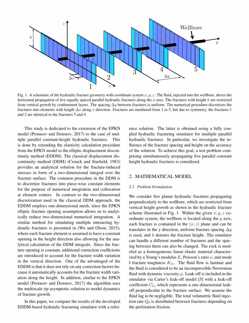
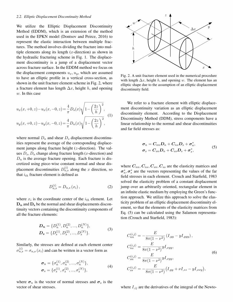
Fig. 1. A schematic of the hydraulic fracture geometry with coordinate system x, y, z. The fluid, injected into the wellbore, drives thehorizontal propagation of five equally spaced parallel hydraulic fractures along the x-axis. The fractures with height h are restrictedfrom vertical growth by confinement layers. The spacing ∆y between fractures is uniform. The numerical procedure discretizes thefractures into elements with length ∆x along x direction. Fractures are numbered from 1 to 5, but due to symmetry, the fractures 1and 2 are identical to the fractures 5 and 4.

This study is dedicated to the extension of the EPKNmodel (Protasov and Donstov, 2017) to the case of mul-tiple parallel constant-height hydraulic fractures. Thisis done by extending the elasticity calculation procedurefrom the EPKN model to the elliptic displacement discon-tinuity method (EDDM). The classical displacement dis-continuity method (DDM) (Crouch and Starfield, 1983)provides an analytical solution for the fracture-inducedstresses in form of a two-dimensional integral over thefracture surface. The common procedure in the DDM isto discretize fractures into piece-wise constant elementsfor the purpose of numerical integration and collocationat element centers. In contrast to the two-dimensionaldiscretization used in the classical DDM approach, theEDDM employs one-dimensional mesh, since the EPKNelliptic fracture opening assumption allows us to analyt-ically reduce two-dimensional numerical integration. Asimilar method for simulating multiple interacting hy-draulic fractures is presented in (Wu and Olson, 2015),where each fracture element is assumed to have a constantopening in the height direction also allowing for the ana-lytical calculation of the DDM integrals. Since the frac-ture opening is constant, additional correction coefficientsare introduced to account for the fracture width variationin the vertical direction. One of the advantaged of theEDDM is that it does not rely on any correction factors be-cause it automatically accounts for the fracture width vari-ation along the height. In addition, similar to the EPKNmodel (Protasov and Donstov, 2017) the algorithm usesthe multiscale tip asymptotic solution to model dynamicsof fracture growth.

In this paper, we compare the results of the developedEDDM-based hydraulic fracturing simulator with a refer-

ence solution. The latter is obtained using a fully cou-pled hydraulic fracturing simulator for multiple parallelhydraulic fractures. In particular, we investigate the in-fluence of the fracture spacing and height on the accuracyof the solution. To achieve this goal, a test problem com-prising simultaneously propagating five parallel constantheight hydraulic fractures is considered.

2. MATHEMATICAL MODEL

2.1. Problem Formulation

We consider five planar hydraulic fractures propagatingperpendicularly to the wellbore, which are restricted fromvertical height growth as shown in the hydraulic fracturescheme illustrated in Fig. 1. Within the given x, y, z co-ordinate system, the wellbore is located along the y axis,each fracture is contained in the (x, z) plane and can betranslates in the y direction, uniform fracture spacing ∆yis used, and h denotes the fracture height. The simulatorcan handle a different number of fractures and the spac-ing between them can also be changed. The rock is mod-eled as a homogeneous linear elastic material character-ized by a Young’s modulusE, Poisson’s ratio ν, and modeI fracture toughness KIc. The fluid flow is laminar andthe fluid is considered to be an incompressible Newtonianfluid with dynamic viscosity µ. Leak-off is included in thesimulator via Carter’s leak-off model [5] with a leak-offcoefficient CL, which represents a one-dimensional leak-off perpendicular to the fracture surface. We assume thefluid lag to be negligible. The total volumetric fluid injec-tion rate Q0 is distributed between fractures depending onthe perforation friction.

2.2. Elliptic Displacement Discontinuity Method

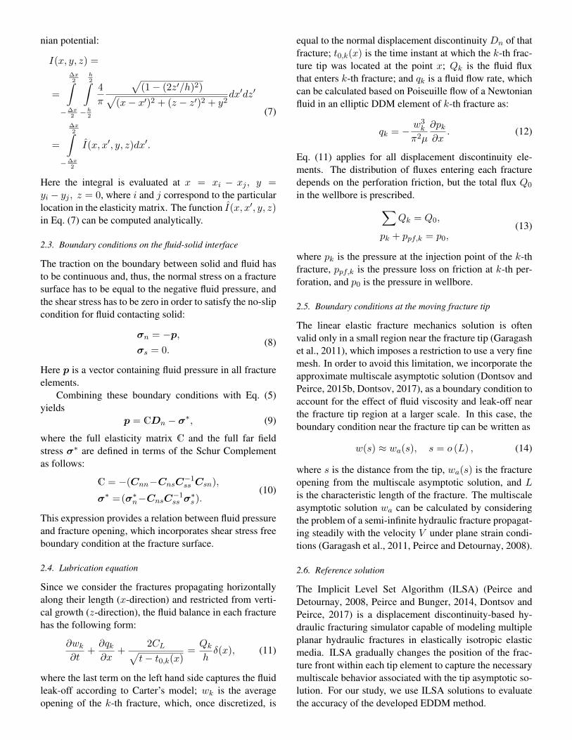
We utilize the Elliptic Displacement DiscontinuityMethod (EDDM), which is an extension of the methodused in the EPKN model (Dontsov and Peirce, 2016) torepresent the elastic interaction between multiple frac-tures. The method involves dividing the fracture into mul-tiple elements along its length (x-direction) as shown inthe hydraulic fracturing scheme in Fig. 1. The displace-ment discontinuity is a jump of a displacement vectoracross fracture surface. In the EDDM method we focus onthe displacement components ux, uy, which are assumedto have an elliptic profile in a vertical cross-section, asshown in the unit fracture element scheme in Fig. 2, wherea fracture element has length ∆x, height h, and openingw. In this case

ux(x,+0, z)−ux(x,−0, z)=4

πDs(x)

√1−(

2z

h

)2

,

uy(x,+0, z)−uy(x,−0, z)=4

πDn(x)

√1−(

2z

h

)2

,

(1)

where normal Dn and shear Ds displacement discontinu-ities represent the average of the corresponding displace-ment jumps along fracture height (z-direction). The val-uesDs, Dn change along fracture length (x-direction) andDn is the average fracture opening. Each fracture is dis-cretized using piece-wise constant normal and shear dis-placement discontinuities D(i)

n,s along the x direction, sothat ith fracture element is defined as

D(i)n,s = Dn,s (xi) , (2)

where xi is the coordinate center of the ith element. LetDn and Ds be the normal and shear displacements discon-tinuity vectors containing the discontinuity components ofall the fracture elements:

Dn = {D(1)n , D(2)

n , ..., D(N)n },

Ds = {D(1)s , D(2)

s , ..., D(N)s }.

(3)

Similarly, the stresses are defined at each element centerσ(i)n,s = σn,s (xi) and can be written in a vector form as

σn = {σ(1)n , σ(2)n , ..., σ(N)n },

σs = {σ(1)s , σ(2)s , ..., σ(N)s },

(4)

where σn is the vector of normal stresses and σs is thevector of shear stresses.

x

y

z

∆x

h

w

Fig. 2. A unit fracture element used in the numerical procedurewith length ∆x, height h, and opening w. The element has anelliptic shape due to the assumption of an elliptic displacementdiscontinuity field.

We refer to a fracture element with elliptic displace-ment discontinuity variation as an elliptic displacementdiscontinuity element. According to the DisplacementDiscontinuity Method (DDM), stress components have alinear relationship to the normal and shear discontinuitiesand far field stresses as:

σn = CnnDn +CnsDs + σ∗n,

σs = CsnDn +CssDs + σ∗s ,(5)

where Cnn,Cns,Csn,Css are the elasticity matrices andσ∗n,σ

∗s are the vectors representing the values of the far

field stresses in each element. Crouch and Starfield, 1983solved the elasticity problem of a constant displacementjump over an arbitrarily oriented, rectangular element inan infinite elastic medium by employing the Green’s func-tion approach. We utilize this approach to solve the elas-ticity problem of an elliptic displacement discontinuity el-ement, so that the elements of the elasticity matrices fromEq. (5) can be calculated using the Salamon representa-tion (Crouch and Starfield, 1983):

C(i,j)nn = − E

8π(1− ν2)(I,yy − yI,yyy) ,

C(i,j)ns =

E

8π(1− ν2)yI,xyy,

C(i,j)sn =

E

8π(1− ν2)yI,xyy,

C(i,j)ss = − E

8π(1− ν2)(I,yy + νI,zz − yI,xxy

),

(6)

where I,ij are the derivatives of the integral of the Newto-

nian potential:

I(x, y, z) =

=

∆x2∫

−∆x2

h2∫

−h2

4

π

√(1− (2z′/h)2)√

(x− x′)2 + (z − z′)2 + y2dx′dz′

=

∆x2∫

−∆x2

I(x, x′, y, z)dx′.

(7)

Here the integral is evaluated at x = xi − xj , y =yi − yj , z = 0, where i and j correspond to the particularlocation in the elasticity matrix. The function I(x, x′, y, z)in Eq. (7) can be computed analytically.

2.3. Boundary conditions on the fluid-solid interface

The traction on the boundary between solid and fluid hasto be continuous and, thus, the normal stress on a fracturesurface has to be equal to the negative fluid pressure, andthe shear stress has to be zero in order to satisfy the no-slipcondition for fluid contacting solid:

σn = −p,σs = 0.

(8)

Here p is a vector containing fluid pressure in all fractureelements.

Combining these boundary conditions with Eq. (5)yields

p = CDn − σ∗, (9)

where the full elasticity matrix C and the full far fieldstress σ∗ are defined in terms of the Schur Complementas follows:

C = −(Cnn−CnsC−1ss Csn),

σ∗ =(σ∗n−CnsC−1ss σ

∗s).

(10)

This expression provides a relation between fluid pressureand fracture opening, which incorporates shear stress freeboundary condition at the fracture surface.

2.4. Lubrication equation

Since we consider the fractures propagating horizontallyalong their length (x-direction) and restricted from verti-cal growth (z-direction), the fluid balance in each fracturehas the following form:

∂wk

∂t+∂qk∂x

+2CL√

t− t0,k(x)=Qk

hδ(x), (11)

where the last term on the left hand side captures the fluidleak-off according to Carter’s model; wk is the averageopening of the k-th fracture, which, once discretized, is

equal to the normal displacement discontinuity Dn of thatfracture; t0,k(x) is the time instant at which the k-th frac-ture tip was located at the point x; Qk is the fluid fluxthat enters k-th fracture; and qk is a fluid flow rate, whichcan be calculated based on Poiseuille flow of a Newtonianfluid in an elliptic DDM element of k-th fracture as:

qk = −w3k

π2µ

∂pk∂x

. (12)

Eq. (11) applies for all displacement discontinuity ele-ments. The distribution of fluxes entering each fracturedepends on the perforation friction, but the total flux Q0

in the wellbore is prescribed.∑Qk = Q0,

pk + ppf,k = p0,(13)

where pk is the pressure at the injection point of the k-thfracture, ppf,k is the pressure loss on friction at k-th per-foration, and p0 is the pressure in wellbore.

2.5. Boundary conditions at the moving fracture tip

The linear elastic fracture mechanics solution is oftenvalid only in a small region near the fracture tip (Garagashet al., 2011), which imposes a restriction to use a very finemesh. In order to avoid this limitation, we incorporate theapproximate multiscale asymptotic solution (Dontsov andPeirce, 2015b, Dontsov, 2017), as a boundary condition toaccount for the effect of fluid viscosity and leak-off nearthe fracture tip region at a larger scale. In this case, theboundary condition near the fracture tip can be written as

w(s) ≈ wa(s), s = o (L) , (14)

where s is the distance from the tip, wa(s) is the fractureopening from the multiscale asymptotic solution, and Lis the characteristic length of the fracture. The multiscaleasymptotic solution wa can be calculated by consideringthe problem of a semi-infinite hydraulic fracture propagat-ing steadily with the velocity V under plane strain condi-tions (Garagash et al., 2011, Peirce and Detournay, 2008).

2.6. Reference solution

The Implicit Level Set Algorithm (ILSA) (Peirce andDetournay, 2008, Peirce and Bunger, 2014, Dontsov andPeirce, 2017) is a displacement discontinuity-based hy-draulic fracturing simulator capable of modeling multipleplanar hydraulic fractures in elastically isotropic elasticmedia. ILSA gradually changes the position of the frac-ture front within each tip element to capture the necessarymultiscale behavior associated with the tip asymptotic so-lution. For our study, we use ILSA solutions to evaluatethe accuracy of the developed EDDM method.

(a) Five hydraulic fractures with 20 m spacing, EDDM results. (b) Five hydraulic fractures with 20 m spacing, ILSA results.

(c) Fracture surface area vs time, spacing 20 m. (d) Fracture surface area vs spacing, time t = 351.

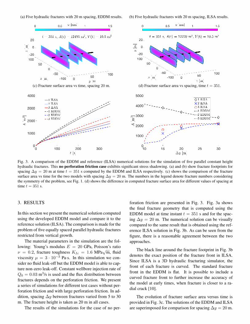
Fig. 3. A comparison of the EDDM and reference (ILSA) numerical solutions for the simulation of five parallel constant heighthydraulic fractures. This no perforation friction case exhibits significant stress shadowing. (a) and (b) show fracture footprints forspacing ∆y = 20 m at time t = 351 s computed by the EDDM and ILSA respectively. (c) shows the comparison of the fracturesurface area vs time for the two models with spacing ∆y = 20 m. The numbers in the legend denote fracture numbers consideringthe symmetry of the problem, see Fig. 1. (d) shows the difference in computed fracture surface area for different values of spacing attime t = 351 s.

3. RESULTS

In this section we present the numerical solution computedusing the developed EDDM model and compare it to thereference solution (ILSA). The comparison is made for theproblem of five equally spaced parallel hydraulic fracturesrestricted from vertical growth.

The material parameters in the simulation are the fol-lowing: Young’s modulus E = 20 GPa, Poisson’s ratioν = 0.2, fracture toughness KIc = 1.6 MPa

√m, fluid

viscosity µ = 3 · 10−3 Pa·s. In this simulation we con-sider no fluid leak-off but the EDDM model is able to cap-ture non-zero leak-off. Constant wellbore injection rate ofQ0 = 0.03 m3/s is used and the flux distribution betweenfractures depends on the perforation friction. We presenta series of simulations for different test cases without per-foration friction and with large perforation friction. In ad-dition, spacing ∆y between fractures varied from 5 to 30m. The fracture height is taken as 20 m in all cases.

The results of the simulations for the case of no per-

foration friction are presented in Fig. 3. Fig. 3a showsthe final fracture geometry that is computed using theEDDM model at time instant t = 351 s and for the spac-ing ∆y = 20 m. The numerical solution can be visuallycompared to the same result that is obtained using the ref-erence ILSA solution in Fig. 3b. As can be seen from thefigure, there is a reasonable agreement between the twoapproaches.

The black line around the fracture footprint in Fig. 3bdenotes the exact position of the fracture front in ILSA.Since ILSA is a 3D hydraulic fracturing simulator, thefront of each fracture is curved. The standard fracturefront in the EDDM is flat. It is possible to include acurved fracture front to further increase the accuracy ofthe model at early times, when fracture is closer to a ra-dial crack [10].

The evolution of fracture surface area versus time isprovided in Fig. 3c. The solutions of the EDDM and ILSAare superimposed for comparison for spacing ∆y = 20 m.

(a) Five hydraulic fractures with ∆y = 20, EDDM results. (b) Five hydraulic fractures with ∆y = 20, ILSA results.

(c) Fracture surface area vs time, ∆y = 20 m. (d) Fracture surface area vs spacing ∆y, time t = 351.

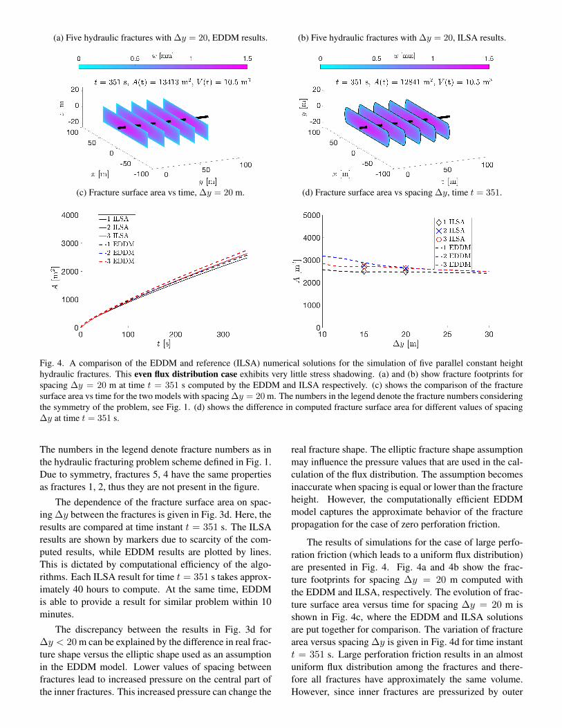
Fig. 4. A comparison of the EDDM and reference (ILSA) numerical solutions for the simulation of five parallel constant heighthydraulic fractures. This even flux distribution case exhibits very little stress shadowing. (a) and (b) show fracture footprints forspacing ∆y = 20 m at time t = 351 s computed by the EDDM and ILSA respectively. (c) shows the comparison of the fracturesurface area vs time for the two models with spacing ∆y = 20 m. The numbers in the legend denote the fracture numbers consideringthe symmetry of the problem, see Fig. 1. (d) shows the difference in computed fracture surface area for different values of spacing∆y at time t = 351 s.

The numbers in the legend denote fracture numbers as inthe hydraulic fracturing problem scheme defined in Fig. 1.Due to symmetry, fractures 5, 4 have the same propertiesas fractures 1, 2, thus they are not present in the figure.

The dependence of the fracture surface area on spac-ing ∆y between the fractures is given in Fig. 3d. Here, theresults are compared at time instant t = 351 s. The ILSAresults are shown by markers due to scarcity of the com-puted results, while EDDM results are plotted by lines.This is dictated by computational efficiency of the algo-rithms. Each ILSA result for time t = 351 s takes approx-imately 40 hours to compute. At the same time, EDDMis able to provide a result for similar problem within 10minutes.

The discrepancy between the results in Fig. 3d for∆y < 20 m can be explained by the difference in real frac-ture shape versus the elliptic shape used as an assumptionin the EDDM model. Lower values of spacing betweenfractures lead to increased pressure on the central part ofthe inner fractures. This increased pressure can change the

real fracture shape. The elliptic fracture shape assumptionmay influence the pressure values that are used in the cal-culation of the flux distribution. The assumption becomesinaccurate when spacing is equal or lower than the fractureheight. However, the computationally efficient EDDMmodel captures the approximate behavior of the fracturepropagation for the case of zero perforation friction.

The results of simulations for the case of large perfo-ration friction (which leads to a uniform flux distribution)are presented in Fig. 4. Fig. 4a and 4b show the frac-ture footprints for spacing ∆y = 20 m computed withthe EDDM and ILSA, respectively. The evolution of frac-ture surface area versus time for spacing ∆y = 20 m isshown in Fig. 4c, where the EDDM and ILSA solutionsare put together for comparison. The variation of fracturearea versus spacing ∆y is given in Fig. 4d for time instantt = 351 s. Large perforation friction results in an almostuniform flux distribution among the fractures and there-fore all fractures have approximately the same volume.However, since inner fractures are pressurized by outer

fractures, they are longer and have larger surface areacompared to the outer ones as can be seen from Fig. 4aand 4b. The EDDM model shows a good agreement withthe reference solution for the case of large perforation fric-tion as can be seen from the evolution of the fracture sur-face area versus time in Fig. 4c. Variation of the fracturesurface area versus spacing ∆y, shown in Fig. 4d, indi-cates that the EDDM agrees with the reference ILSA solu-tion for the various spacings considered. The fact that theEDDM model gives more accurate results for large per-foration friction than zero perforation friction shows thatelliptic fracture shape assumption may influence the fluxdistribution calculation.

4. SUMMARY

This paper presents a developed EDDM hydraulic fractur-ing simulator for modeling simultaneous growth of mul-tiple parallel constant height hydraulic fractures. Thissimulator is the extension of the original EPKN simula-tor for a single fracture. One of the basic assumptionsis that fracture has normal and shear displacement dis-continuities of elliptical shape, which allows us to reducethe elasticity problem from a two-dimensional to a one-dimensional, which leads to the elliptic displacement dis-continuity method. The other feature of the algorithm isthe multiscale tip asymptotic solution that can accuratelycapture effects of fluid viscosity and fracture toughness,which increases computational efficiency of the developedsimulator by allowing a coarser mesh. The EDDM simu-lator uses a fixed mesh algorithm, which can allow for afurther extension to model curved fractures. In order toverify the developed model, we compare it to the fully3D hydraulic fracturing simulator for multiple parallel hy-draulic fractures. In particular, we consider five uniformlyspaced parallel constant height fractures. We investigatethe effect of perforation friction and spacing on the re-sults. The EDDM model agrees with the reference solu-tion when spacing between fractures is greater than thefracture height. A discrepancy in the flux distribution ap-pears for the zero perforation friction case when the frac-ture spacing becomes comparable or smaller than the frac-ture height. However, the EDDM model can handle theconsidered problem within several minutes on a regularcomputer.

ACKNOWLEDGEMENTS

Start up funds provided by the University of Houston aregreatly acknowledged.

REFERENCES

1. Abou-Sayed, A.S., D.E. Andrews, and I.M. Buhidma.1989. Evaluation of oily waste injection below the per-mafrost in Prudhoe Bay field. In Proceedings of theCalifornia Regional Meetings, Bakersfield, CA, Society ofPetroleum Engineers, pages 129-142.

2. Adachi, J., E. Siebrits, A. Peirce, and J. Desroches. 2007.Computer simulation of hydraulic fractures. Int. J. RockMech. Min. Sci., 44:739–757.

3. Adachi, J. and A.P. Peirce. Asymptotic Analysis of an Elas-ticity Equation for a Finger-Like Hydraulic Fracture 2008.Journal of Elasticity, 90, 43-69.

4. Brown, D.W. 2000. A hot dry rock geothermal energyconcept utilizing supercritical co2 instead of water. In Pro-ceedings of Twenty-Fifth Workshop on Geothermal Reser-voir Engineering Stanford University, Stanford, California.

5. Carter, E.D. 1957. Optimum fluid characteristics for frac-ture extension. In Drilling and production practices, 261–270.

6. Crouch, S.L. and A.M. Starfield. 1983. Boundary elementmethods in solid mechanics. London: George Allen andUnwin.

7. Dontsov, E.V. 2017. An approximate solution for a planestrain hydraulic fracture that accounts for fracture tough-ness, fluid viscosity, and leak-off. Int. J. Fract., 205:221–237.

8. Dontsov, E. and A. Peirce. 2015a. An enhanced pseudo-3D model for hydraulic fracturing accounting for viscousheight growth, non-local elasticity, and lateral toughness.Eng. Frac. Mech., 142:116–139.

9. Dontsov, E. and A. Peirce. 2015b. A non-singular inte-gral equation formulation to analyze multiscale behaviourin semi-infinite hydraulic fractures. J. Fluid. Mech., 781:R1.

10. Dontsov, E.V. and A. P. Peirce. 2016. Comparison oftoughness propagation criteria for blade-like and pseudo-3d hydraulic fractures. Eng. Frac. Mech., 160:238–247.

11. Dontsov, E.V and A.P. Peirce. 2017. A multiscale Im-plicit Level Set Algorithm (ILSA) to model hydraulic frac-ture propagation incorporating combined viscous, tough-ness, and leak-off asymptotics. Comp.Meth. in Appl. Mech.and Eng., 313, pp. 53-84.

12. Economides, M.J. and K.G. Nolte, editors. 2000. Reser-voir Stimulation. John Wiley & Sons, Chichester, UK, 3rdedition.

13. Garagash D.I., E. Detournay, and J.I. Adachi. 2011. Multi-scale tip asymptotics in hydraulic fracture with leak-off. J.Fluid Mech., 669:260–297.

14. Jeffrey, R.G. and K.W. Mills. 2000. Hydraulic fracturingapplied to inducing longwall coal mine goaf falls. In PacificRocks 2000, Balkema, Rotterdam, pages 423-430.

15. Kresse, O., X. Weng, H. Gu, and R. Wu. 2013. Numer-ical modeling of hydraulic fracture interaction in complexnaturally fractured formations. Rock Mech. Rock Eng., 46:555–558.

16. McClure, M.W. and M.D. Zoback. 2013. Computa-tional investigation of trends in initial shut-in pressure dur-ing multi-stage hydraulic stimulation in the barnett shale.In Proceedings of the 47nd U.S. Rock Mechanics Sympo-sium. San Francisco, CA, USA.

17. Nordgren, R.P. 1972. Propagation of vertical hydraulicfractures. In Soc. Petrol. Eng. J., pages 306–314.

18. Olson, J.E. 2008. Multi-fracture propagation modeling:Applications to hydraulic fracturing in shales and tight gassands. In Proceedings of the 42nd U.S. Rock MechanicsSymposium. San Francisco, CA, USA.

19. Peirce, A.P. 2015 Modeling multi-scale processes in hy-draulic fracture propagation using the implicit level set al-gorithm. Comp. Meth. in Appl. Mech. and Eng., 283:881-908.

20. Peirce, A.P. and A.P. Bunger. 2014 Interference fracturing:Non-uniform distributions of perforation clusters that pro-mote simultaneous growth of multiple hydraulic fractures.SPE 172500.

21. Peirce, A. and E. Detournay. 2008. An implicit level setmethod for modeling hydraulically driven fractures. Com-put. Methods Appl. Mech. Engrg., 197:2858–2885.

22. Perkins, T.K. and L.R. Kern. 1961. Widths of hydraulicfractures. In J. Pet. Tech. Trans. AIME, pages 937–949.

23. Protasov, I. and E. Donstov. 2017 A comparison ofnon-local elasticity models for a blade-like hydraulic frac-ture In Proceedings of the 51st U.S. Rock Mechan-ics/Geomechanics Symposium, San Francisco, CA, USA

24. Wu, K., J. Olson, M.T. Balhoff, and W. Yu. 2015. Numer-ical analysis for promoting uniform development of simul-taneous multiple fracture propagation in horizontal wells.In Proceedings of the SPE Annual Technical Conferenceand Exhibition, SPE-174869-MS.

25. Wu, K., J. Olson. 2015. A simplified three-dimensional dis-placement discontinuity method for multiple fracture sim-ulations. Int. J. Frac. 193(2)