ARITHMETIC THETA LIFTS AND THE ARITHMETIC

GAN–GROSS–PRASAD CONJECTURE FOR UNITARY GROUPS

HANG XUE

Abstract. We propose a precise formula relating the height of certain diagonal cycles on the

product of unitary Shimura varieties and the central derivative of some tensor product L-functions.

This can be viewed as a refinement of the arithmetic Gan–Gross–Prasad conjecture. We use the

theory of arithmetic theta lifts to prove some endoscopic cases of it for U(2)×U(3).

Contents

1. Introduction 2

1.1. The conjecture and the main result 3

1.2. The method 5

1.3. Organization of the paper 8

1.4. Notation 8

1.5. Measures 9

2. The height pairing 10

2.1. Trivializing cohomology classes 10

2.2. Arithmetic intersection theory 11

2.3. Height pairing: Generalities 12

2.4. Height pairing: the case of a product of a curve and a surface 13

3. Theta lifts 15

3.1. Weil representations 15

3.2. The archimedean case 16

3.3. Doubling zeta integrals 17

3.4. A duality property of doubling zeta integrals 19

4. Arithmetic theta lifts 23

4.1. Shimura varieties attached to incoherent unitary groups 23

4.2. Hecke actions 24

4.3. Generating series 25

4.4. Pullback of generating series 27

4.5. Arithmetic theta lifts 27

4.6. Hecke correspondences as arithmetic theta lifts 30

Date: June 12, 2018.

1

5. The arithmetic GGP conjecture 32

5.1. The conjecture 32

5.2. Projectors 34

5.3. Proof of Theorem 5.3: geometry 36

5.4. Proof of Theorem 5.3: arithmetic seesaw 38

Appendix A. The Gross–Zagier formula 40

A.1. Formulae on quaternion algebras 40

A.2. Unitary groups in two variables 42

A.3. The formula on the unitary groups 44

References 46

1. Introduction

In 1980s, Gross–Zagier [GZ86] established a formula that relates the Neron–Tate height of Heeg-

ner points on modular curves to the central derivative of certain L-functions associated to modular

forms. Around the same time, Waldspurger proved a formula, relating toric periods of modular

forms to the central value of certain L-functions. Gross put both of these formula in the framework

of representation theory in his MSRI lecture in 2001 [Gro04]. In this framework, the formula of

Waldspurger concerns the toric periods of automorphic forms on quaternion algebras, while the

formula of Gross–Zagier maybe viewed as a formula for the “periods” of “automorphic forms” on

the incoherent quaternion algebras. The proof of the most general form of the Gross–Zagier formula

given in [YZZ13] has been largely inspired by the proof of Waldspurger’s formula.

Gross–Prasad [GP92] formulated a conjecture which generalizes the work of Waldspurger to

relate the nonvanishing of SO(n)-periods of automorphic forms on SO(n) × SO(n + 1) and the

nonvanishing of the central value of certain Rankin–Selberg L-functions, with Waldspurger’s for-

mula being the case n = 2. Gan, Gross and Prasad [GGP12] further generalized this framework

to include all classical groups. These conjectures are usually referred to as the Gan–Gross–Prasad

(GGP) conjectures. Parallel to the periods of automorphic forms, a conjectural generalization

of the Gross–Zagier formula to higher-dimensional Shimura varieties has been proposed, for in-

stance, in [GGP12, Zha12]. These are generally referred to as the arithmetic Gan–Gross–Prasad

conjectures, or arithmetic GGP conjectures for short.

The goal of this paper is to prove some endoscopic cases of the arithmetic GGP conjecture for

U(2)×U(3) using theta correspondences and arithmetic theta lifts of Kudla [Kud04] and Liu [Liu11a,

Liu11b]. In principle, our argument generalizes to the case of all n, yielding a relation among the

GGP conjecture for U(n) × U(n), Liu’s conjecture on the arithmetic inner product formula and

some endocopic cases of the arithmetic GGP conjecture for U(n)×U(n+1). We stick to the case of

U(2)×U(3), as if n > 2, Liu’s conjectural arithmetic inner product formula is not available currently,2

and the GGP conjecture for U(n)×U(n) is known only in some cases which is not sufficient for the

application of the method of this paper. Moreover, in this situation, we can formulate our main

result unconditionally, without appealing to the standard conjectures of Beilinson and Bloch.

We hope that the results of this paper provide some further motivation, in addition to the already

amply demonstrated ones, for the study of the GGP conjecture for U(n)×U(n) and the arithmetic

inner product formulae.

A byproduct of our investigation is that it enables us to predict a precise conjectural formula

for the height and the central derivative of L-functions for U(n) × U(n + 1), in the style of the

Ichino–Ikeda’s conjecture [II10, Har14], as a refinement to the original Gross–Prasad conjecture.

Our main result is to verify this formula for U(2)×U(3) in some endoscopic cases. In the appendix,

we check that the case of U(1) × U(2) is compatible with the main result of [YZZ13]. It turns

out that even the case U(1) × U(2) is not merely a triviality since the formulation of the results

in [YZZ13] is different from ours. This also provides strong evidence that the complicated constant

involving the measures and the power of two in the precise formula is correct.

1.1. The conjecture and the main result. Let us briefly recall the arithmetic GGP conjecture

for U(n)×U(n+ 1). The details will be given in Section 5. Let F be a totally real field and E/F

a CM extension. Let W ⊂ V be a pair of incoherent Hermitian spaces over AE of rank n and

n+ 1 respectively. Assume that W and V are both positive definite at all infinite places of E. Put

H = U(W) and G = U(W)×U(V). These are the reductive groups over AF . There is a (projective

system of) Shimura variety Y of dimension n−1 (resp. X of dimension n) attached to U(W) (resp.

U(V)). Put M = Y ×X. We have an embedding Y → X induced by the inclusion W ⊂ V. Thus

we have a diagonal embedding Y → M and in this way Y defines a cycle of codimension n in M ,

which we denote by y. Let cl : Chn(M) → H2n(M) be the cycle class map and Chn(M)0 be the

kernel of cl which consists of cohomologically trivial cycles. It is expected that there is a Hecke

equivariant projection Chn(M)→ Chn(M)0. We assume such a projection exists and denote by y0

the image of y under this projection. We are going to construct this y0 when n = 1 or 2.

Let A be the set of irreducible admissible representations of G(AF ) which appear in H2n−1(M).

Note that by definition G(F∞) acts trivially on H2n−1(M). Then we have a surjective map

C∞c (G(AF,f ))→⊕π∈A

π ⊗ π.

Let us fix an inner product on π so as to identify π with π. Let π ∈ A and ϕ ∈ π. We choose

a function t ∈ C∞c (G(AF,f )) which maps to ϕ ⊗ ϕ. Let T (t) be the Hecke correspondence on M

given by t.

We need to invoke the Beilinson–Bloch height pairing. This is a highly conjectural pairing for

the cohomologically trivial cycles. To proceed, we propose the following hypothesis.

Hypothesis 1.1. We have the following hypothesis of Beilinson and Bloch.3

(1) The height pairing 〈−,−〉BB is well-defined, cf. the Hypothesis (BB1) and (BB2) in Sec-

tion 2.3.

(2) Suppose that S is a smooth projective variety defined over a number field and δ be a corre-

spondence on S. If δ∗ acts trivially on H2r−1(S), then it acts trivially on Chr(S)0.

The arithmetic GGP conjecture then predicts the following identity

〈T (t)∗y0, y0〉BB = (∗)L′(1

2, π),

where

– (∗) is some explicit nonzero constant which we will specify in Conjecture 5.1;

– L(s, π) is a certain tensor product L-function attached to π.

By Hypothesis 1.1, the left hand side does not depend on the choice of t, but only on ϕ. Moreover

the height pairing is well-defined.

Theorem 1.2 (provisional form). Assume n = 2 and Hypothesis 1.1. Assume that

– the Shimura varieties in question are all projective, e.g. F 6= Q;

– both automorphic representations on U(3) and U(2) are theta lifts from the quasi-split U(2).

Then the arithmetic GGP conjecture for U(2)×U(3) holds.

We refer the readers to Theorem 5.2 for the precise statement of the theorem.

One drawback of this formulation of the theorem is that it is conditional on Hypothesis 1.1 for

the 3-folds, especially (2), which is impossible to check even for some very simple varieties, e.g.

triple product of smooth projective curves. Therefore we formulate the main result of this paper in

a different way, cf. Theorem 5.3. Under Hypothesis 1.1, these two formulations are equivalent. In

the formulation of Theorem 5.3, we do not assume Hypothesis 1.1, but only the existence of regular

models of X and X × Y . This is of course expected for all surfaces by the conjectural resolution

of singularities. In practice, this assumption can be verified when the level of the Picard modular

surface is simple.

The main result of this paper should be considered as some “degenerate” case of the arithmetic

Gan–Gross-Prasad conjecture. In fact, let us write π = π2π3 where π2 (resp. π3) is an admissible

representation of U(2) (resp. U(3)). Under the assumption of theorem, there are two irreducible

cuspidal automorphic representations σ1 and σ2 such that π2 (resp. π3) is a theta lift of σ1 (resp.

σ2), as abstract representations. Therefore the L-function factorizes as

L(s, π) = L(s, π3 × π2) = L(s, σ1 × σ2)L(s, σ1).

Here L(s, σ1 × σ2) is some tensor product L-function of σ1 and σ2 and L(s, σ1) is the standard

L-function of σ1 defined by the doubling zeta integrals. There are some twists in these L-functions,

but just to fix ideas, let us ignore this issue here. Under our assumption, L(12 , σ1) = 0 as the sign

4

of the functional equation is −1. Therefore

L′(1

2, π) = L(

1

2, σ1 × σ2)L′(

1

2, σ1).

This means that the picture on the L-function side is essentially known. More precisely, L(12 , σ1×σ2)

is the one appearing in the GGP conjecture for U(2)× U(2) and L′(12 , σ1) is the one appearing in

Liu’s arithmetic inner product formula. So it is not too surprising that the height pairing on M

should be reduced to some known height pairings, i.e. a height pairing of arithmetic theta lifts on

Y . Indeed, this was the very first observation which led to this paper.

One should also compare Theorem 1.2 to the “degenerate” case of the formula for the central

derivative of the triple product L-function [YZZ]. Namely, using the same technique as in this paper,

plus the arithmetic inner product formula of Kudla–Rapoport–Yang [KRY06], we should be able

to deduce certain degenerate cases of central derivative formula of the triple product L-function,

in particular [YZZ, Corollary 1.3.2].

1.2. The method. Jacquet–Rallis proposed a relative trace formula approach to the GGP conjec-

ture for U(n)×U(n+ 1). This is by far the most successful approach. It proves the (nonvanishing

part) of the GGP conjecture under the assumption that the representation in question is supercus-

pidal at some split place [Zha14b, Xue]. Inspired by this approach, W. Zhang proposed a relative

trace formula to attack the arithmetic GGP conjecture for U(n) × U(n + 1) [Zha12]. As a first

step, an arithmetic fundamental lemma was conjectured and proved in the case of U(2) × U(3).

A smooth transfer conjecture has been formulated in [RSZ] and verified for U(2) × U(3) in some

special cases. These results strongly support the solidity of the relative trace formula approach.

There is a different approach to the GGP conjecture via theta correspondences. This approach

proves the GGP conjecture for SO(2)× SO(3) and SO(3)× SO(4) in full generality and is capable

of obtaining some endoscopic cases of U(n) × U(n + 1). Due to technical limitations, mainly

the lack of a fine spectral expansion, the relative trace formula only handles the case where the

automorphic representations of U(n)×U(n+ 1) are stable, i.e. their base change remain cuspidal.

Contrary to this, the theta correspondence approach has the limitation that, besides some low rank

situations, it only handles certain endoscopic cases. So at present, these two methods seem to be

complementary to each other. Of course, the relative trace formula approach is much more powerful

and has the potential of proving the conjectures in full generality. Nevertheless, the argument via

theta correspondence is still useful, for its clarity and simplicity. Moreover, the method of theta

correspondences yields directly precise identities between central L-values and periods.

In this paper, we use arithmetic theta lifts to attack the arithmetic GGP conjecture. We in

fact state a more precise version of the conjecture. It is clear that such a formulation is directly

borrowed from the conjecture of Ichino–Ikeda [II10]. Our method is again largely inspired by the

theta correspondence approach to the GGP conjecture.5

We now describe our method. First we introduce some notation. Let H be the quasi-split unitary

group in two variables. Then we have a Weil representation ω of H(AF )× U(V)(AF ), realized on

S(V). It depends on a nontrivial additive character ψ of F\AF and a multiplicative character χ

of E×\A×E . Write π = π2 π3 where π2 (resp. π3) is an irreducible admissible representation of

U(W)(AF ) (resp. U(V)(AF )). We may assume that ϕ = ϕ2 ⊗ ϕ3 where ϕi ∈ πi, i = 2, 3. Then

T (t) = T (t2)×T (t3) where T (t2) (resp. T (t3)) is a Hecke operator on Y (resp. X). By assumption,

there is an irreducible cuspidal automorphic representation σ2 of H(AF ) such that π3 is a theta

lift of σ2 (as an abstract representation). This means that there is a nonzero H(AF )×U(V)(AF )-

equivariant map σ2 ⊗ ω → π3. Let us fix such a map and choose f2 ∈ σ2 and φ3 ∈ S(V) so that

(f2, φ3) maps to ϕ3. We may further assume that ϕ3 has the property that φ3 can be chosen to be

of the form φ2 ⊗ φ1 where φ2 ∈ S(W) and φ1 ∈ S(AE). The proof of Theorem 1.2 now proceeds

in the following steps. For brevity, we do not pay much attention on the constants, expect for the

central values and derivatives of the L-functions.

(1) Interpreting Hecke correspondences in terms of arithmetic theta liftings, cf. Subsection 4.6.

Let Θ = Θφ3f2

be the arithmetic theta lift from H(AF ) to X in the sense of Liu [Liu11a].

This is a (formal sum of) divisor(s) on X. We have that T (t3) and Θ×Θ define the same

cohomology class in H4(X×X), cf. Proposition 4.10. Therefore by Hypothesis 1.1, we have

〈(T (t2)× T (t3))∗y0, y0〉BB = 〈(T (t2)×Θ×Θ)∗y0, y0〉BB.

(2) Reducing the height pairing on Y ×X to a height pairing on Y , cf. Subsection 2.4. A little

computation shows that we have

〈(T (t2)×Θ×Θ)∗y0, y0〉BB = 〈T (t2)∗(Θ|Y )0, (Θ|Y )0〉NT,

where 〈−,−〉NT stands for the Neron–Tate height pairing on Y and (Θ|Y )0 is the projection

of Θ|Y to the cohomologically trivial part of Ch1(Y ). We will prove that the height pairing

on the left hand side is well-defined, without assuming Hypothesis 1.1.

(3) A pullback formula for Θ, cf. Subsection 4.4. Let Z(h, φ2) be the generating series on

H(AF ) valued in Ch1(Y ) (c.f. [Liu11a]) and Z(h, φ2)0 be its projection the cohomologically

trivial part of Ch1(Y ). Let θ(h, φ1) be the theta function on H(AF ). We have

(Θ|Y )0 =

∫H(AF )

f2(h)Z(h, φ2)0θ(h, φ1)dh.

An analogous result for the generating series on the symplectic groups and valued in the

Chow group of orthogonal Shimura varieties was proved in [YZZ09].

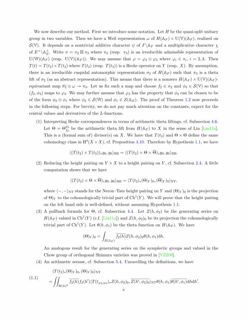
(4) An arithmetic seesaw, cf. Subsection 5.4. Unravelling the definitions, we have

(1.1)

〈T (t2)∗(Θ|Y )0, (Θ|Y )0〉NT

=

∫∫H(A)2

f2(h)f2(h′)〈T (tϕ2,ϕ2)∗Z(h, φ2)0, Z(h′, φ2)0〉NTθ(h, φ1)θ(h′, φ1)dhdh′.

6

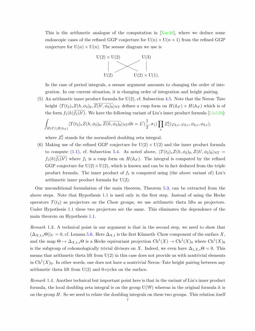
This is the arithmetic analogue of the computation in [Xue16], where we deduce some

endoscopic cases of the refined GGP conjecture for U(n)×U(n+ 1) from the refined GGP

conjecture for U(n)×U(n). The seesaw diagram we use is

U(2)×U(2) U(3)

U(2) U(2)×U(1).

In the case of period integrals, a seesaw argument amounts to changing the order of inte-

gration. In our current situation, it is changing order of integration and height pairing.

(5) An arithmetic inner product formula for U(2), cf. Subsection 4.5. Note that the Neron–Tate

height 〈T (t2)∗Z(h, φ2)0, Z(h′, φ2)0〉NT defines a cusp form on H(AF ) ×H(AF ) which is of

the form f1(h)f1(h′). We have the following variant of Liu’s inner product formula [Liu11b]:∫H(F )\H(AF )

〈T (t2)∗Z(h, φ2)0, Z(h, φ2)0〉NTdh = L′(1

2, σ1)

∏v

Z\v(ϕ2,v, ϕ2,v, φ2,v, φ2,v),

where Z\v stands for the normalized doubling zeta integral.

(6) Making use of the refined GGP conjecture for U(2) × U(2) and the inner product formula

to compute (1.1), cf. Subsection 5.4. As noted above, 〈T (t2)∗Z(h, φ2)0, Z(h′, φ2)0〉NT =

f1(h)f1(h′) where f1 is a cusp form on H(AF ). The integral is computed by the refined

GGP conjecture for U(2)×U(2), which is known and can be in fact deduced from the triple

product formula. The inner product of f1 is computed using (the above variant of) Liu’s

arithmetic inner product formula for U(2).

Our unconditional formulation of the main theorem, Theorem 5.3, can be extracted from the

above steps. Note that Hypothesis 1.1 is used only in the first step. Instead of using the Hecke

operators T (t3) as projectors on the Chow groups, we use arithmetic theta lifts as projectors.

Under Hypothesis 1.1 these two projectors are the same. This eliminates the dependence of the

main theorem on Hypothesis 1.1.

Remark 1.3. A technical point in our argument is that in the second step, we need to show that

(∆X,1,∗Θ)|Y = 0, cf. Lemma 5.6. Here ∆X,1 is the first Kunneth–Chow component of the surface X,

and the map Θ 7→ ∆X,1,∗Θ is a Hecke equivariant projection Ch1(X) → Ch1(X)0 where Ch1(X)0

is the subgroup of cohomologically trivial divisors on X. Indeed, we even have ∆1,X,∗Θ = 0. This

means that arithmetic theta lift from U(2) in this case does not provide us with nontrivial elements

in Ch1(X)0. In other words, one does not have a nontrivial Neron–Tate height pairing between any

arithmetic theta lift from U(2) and 0-cycles on the surface.

Remark 1.4. Another technical but important point here is that in the variant of Liu’s inner product

formula, the local doubling zeta integral is on the group U(W) whereas in the original formula it is

on the group H. So we need to relate the doubling integrals on these two groups. This relation itself7

and its proof may be of independent interest. It turns out that such a relation is a generalization of

the fact that the equal rank local theta correspondence preserves the formal degree in the case of

discrete series representations. We refer the readers to Subsection 3.4 for a more detailed discussion.

1.3. Organization of the paper. This paper is organized as follows. In Section 2, we review how

to construct cohomologically trivial cycle classes and the theory of height pairing. As the theory

of height pairing is still highly conjectural, to work with it, we need some working hypothesis. We

state these hypothesis in this section. We also study the height pairing on the product of a curve

and a surface. The main result is Proposition 2.2. It proves that in some special cases, the height

pairing of 1-cycles on the product of a surface and a curve is well defined and can be reduced to

the Neron–Tate height pairing on a curve. In Section 3, we review the theory of theta lifts and

doubling zeta integrals. The new result is Proposition 3.4, which handles the second technical

point mentioned in the previous subsection. In Section 4, we review the theory of arithmetic

theta lifts following [Liu11a, Liu11b]. We prove two results. The first is an identity between the

Hecke correspondences and the arithmetic theta lifts. The second is a variant of Liu’s arithmetic

inner product formula. The key input in this variant is Proposition 3.4. Section 5 contains the

main results of this paper. We first state the precise form of the arithmetic GGP conjecture.

Then combining all results from the previous sections, we prove this conjecture for U(2) × U(3)

in the endoscopic case. We state two versions of our main theorem. The version depending on

Hypothesis 1.1 is Theorem 5.2. The unconditional version is Theorem 5.3. In the appendix, we

check that the arithmetic GGP conjecture, in its precise form, is compatible with the Gross–Zagier

formula proved in [YZZ13].

1.4. Notation. Throughout this paper, we fix the following notation and convention.

– Let F be a number field and E/F a quadratic extension. We write AF,f for the group of

finite adeles and F∞ =∏v|∞ Fv. We fix a nontrivial additive character ψ : F\AF → C×,

such that for each archimedean place v of F , ψv(x) = e2πix. Put ψE(x) = ψ(12 TrE/F x).

Let η : F×\A×F → ±1 be the quadratic character associated to the extension E/F .

– By a Hermitian space V over AE , we mean a restricted tensor product V = ⊗Vv where Vvis a Hermitian space over Ev. It is said to be coherent if there is a Hermitian space V over

E so that V = V ⊗ AE . It is said to be incoherent if such a V does not exist.

– By the Hermitian space AE (over AE), we mean the one dimensional hermitian space over

AE , with the Hermitian inner product given by (x, y) 7→ xy.

– For any algebraic group G over F , we put [G] = G(F )\G(AF ).

– For any algebraic variety X of F , we let Ch∗(X), Pic(X), H∗(X) be the Chow group, the

Picard group of X and the (Betti) cohomology group of X(C) (for some embedding F → Cwhich is clear from the context). Without saying explicitly to the contrary, they all have Ccoefficients. Thus we may take complex conjugation of elements in these groups.

8

1.5. Measures. Let us fix some measures. Recall that we have fixed a nontrivial additive character

ψ : F\AF → C×.

For any place v of F , let V be a Hermitian space over Ev of dimension n. Let u(V ) be the Lie

algebra of U(V ). Let cv : u(V )→ U(V ) be the Cayley transform, namely,

cv(X) = (1 +X)(1−X)−1, X ∈ u(V ).

We have a self-dual measure on u(V ) and we let d′hv be the unique measure on U(V ) so that the

Caylay transform is measure preserving. Suppose that n = 2r. Then this measure satisfies the

property that∫Herm2r(Ev)

(∫V 2r

φ(x)ψ(TrnQ(x))dx

)ψ(−TrnQ)dn = γV

∫U(V )(Fv)

φ(h−1v xQ)d′hv,

where Herm2r stands for the space of 2r × 2r Hermitian matrices, dT is the self-dual measure on

Herm2r, and xQ is any fixed element in V 2r with Q(x) = Q where Q(x) stands for the moment

matrix of x. Put

dhv = L(1, ηv)ζFv(2) · · ·L(n, ηnv )d′hv.

We shall call d′hv the unnormalized local measure and dhv the normalized local measure. Thus

the normalized local measure coincides with the measure d′hp in [Liu12, Definition 4.3.3] (in the

notation there).

Let V be a Hermitian space over E of dimension n. Then the Tamagawa measure on [U(V )]

equals

(L(1, η) · · ·L(n, ηn))−1∏v

dhv.

Let V be an incoherent Hermitian space over AE of dimension n. By abuse of terminology, we call

the measure

(L(1, η)ζ(2) · · ·L(n, ηn))−1∏v

dhv

the Tamagawa measure on U(V)(AF ).

Let K ⊂ U(V )(AF,f ) an open compact subgroup. By volK, we mean the volume of K with

respect to the measure

(2L(1, η)ζ(2) · · ·L(n, ηn))−1∏

v finite

dhv,

where dhv is the normalized local measure at v. This coincides with the measure given in [Liu11a,

Definition 4.3.3]. The volume of K computed using other measures will be denoted by vol′K.

Acknowledgements. I would like to thank Xinyi Yuan, who carefully explained many subtle points

concerning Shimura varieties and height pairings. This paper would not have existed without his

constant help. The appendix was prepared while I was visiting him at Berkeley. I also thank Yifeng

Liu and Wei Zhang for many helpful discussions. I am grateful to Shouwu Zhang for his interest

in this work and the constant support.9

2. The height pairing

The goal of this section is to review the (conjectural) height pairing of Beilinson–Bloch. We also

study the height pairing on a product of a curve and a surface. In this case, the height pairing

can be defined under some mild conditions for a large class of cohomologically trivial cycles. We

suggest the readers look at only Subsection 2.1 and the statement of Proposition 2.2 for the first

reading.

2.1. Trivializing cohomology classes. In this subsection, we review how to construct cohomo-

logically trivial cycle classes in some low dimensional cases.

Let X be a smooth projective variety over F of dimension n. Let Chi(X) (resp. Chi(X)) be

C-vector space of codimension i (resp. dimension i) cycles on X. There is an intersection paring

between Ch∗(X) and Ch∗(X), which we denote by α · β, α ∈ Ch∗(X), β ∈ Ch∗(X).

Let cl : Chi(X)→ H2i(X) be the cycle class map and Chi(X)0 be the kernel of cl. It is expected

that there is a splitting

Chi(X) ' Chi(X)0 ⊕ Im cl .

In the case X being a Shimura variety, it is expected that this splitting is Hecke equivariant. If X

is the Shimura variety attached to a unitary group, W. Zhang recently constructs a candidate of

it using Hecke operators. His construction indeed gives a splitting if we assume Hypothesis 1.1. In

certain low dimensional cases, we may also use Kunneth–Chow decomposition to construct such

a splitting. Even though it is very hard to show the existence of such a decomposition in higher

dimensions, in the low dimensional cases, it has the advantage of being concrete and geometric. The

idea of using Kunneth–Chow decomposition to trivialize cohomology classes in the low dimensional

cases is also due to W. Zhang [Zha].

Let ∆ be the diagonal cycle in X ×X. By a Kunneth–Chow decomposition, we mean a sum

∆ = ∆X,0 + ∆X,1 + · · ·∆X,2n ∈ Chn(X ×X),

such that the natural map ∆X,i,∗ : H∗(X)→ H∗(X) is the projection to the i-th component. We call

∆X,i the i-th Kunneth–Chow component of X. When there is no confusion, we write ∆i instead

of ∆X,i. The existence of the Kunneth–Chow decomposition is one of the standard conjectures

on algebraic cycles. The essentially known cases are curves and surfaces. Let z ∈ Chr(X) be a

codimension r cycle on X. Then it follows from the definition of the Kunneth–Chow decomposition

that ∆X,2r−1,∗z ∈ Chr(X)0. This defines a map

Chr(X)→ Chr(X)0, z 7→ ∆X,2r−1,∗z,

and for some good choice of the Kunneth–Chow decomposition, it is expected to be the splitting

that we are looking for.

Let us now recall the construction of Kunneth–Chow decomposition in the low dimensional cases.10

Suppose that n = 1, i.e. X is a smooth projective curve. Choose an ample class ξ ∈ Pic(X) of

degree one and put

∆0 = X × ξ, ∆2 = ξ ×X, ∆1 = ∆−∆0 −∆2.

It is well-known (and easy to check) that ∆ = ∆0 + ∆1 + ∆2 is a Kunneth–Chow decomposition.

Suppose that n = 2, i.e. X is a smooth projective surface. Choose an ample class ξ ∈ Pic(X)

and let e = (deg ξ · ξ)−1(ξ · ξ) ∈ Ch2(X). Let Alb(X) be the Albanese variety of X and Pic0(X) be

the neutral component of the Picard variety of X. Let α : Pic0(X)→ Alb(X) be the isogeny given

by L 7→ L · ξ and α∨ : Alb(X)→ Pic0(X) the dual isogeny. Assume that the degree of α is d. Let

j : X → Pic0(X) be the composition of the natural map X → Alb(X) given by x 7→ x− e and the

isogeny α∨. Then we have a morphism

j × 1 : X ×X → Pic0(X)×X,

where 1 stands for the identity morphism. Let P be the Poincare bundle on Pic0(X) × X and

β = (j × 1)∗P. Put

∆0 = X × e, ∆1 =1

dp∗1ξ · β, ∆3 = t∆1, ∆4 = e×X, ∆2 = ∆−∆0 −∆1 −∆3 −∆4,

where p1 : X ×X → X is the projection to the first factor. Then ∆ = ∆0 + ∆1 + ∆2 + ∆3 + ∆4 is

a Kunneth–Chow decomposition for X.

Suppose that X = C × S where C is a smooth projective curve and S is a smooth projective

surface. Choose an ample class ξ ∈ Pic(X). Then we have a Kunneth–Chow decomposition for S

(with respect to ξ) and C (with respect to ξ|C) respectively. Let

∆X,i =

i∑j=0

∆C,j ×∆S,i−j , i = 0, 1, · · · , 6

Then ∆X =∑6

i=0 ∆X,i is a Kunneth–Chow decomposition.

2.2. Arithmetic intersection theory. By an arithmetic variety of dimension n+ 1 over oF , we

mean an integral scheme X , projective and flat over oF such that the generic fiber XF = X ×SpecF

is smooth. We mainly follow the exposition in [Zha10, Section 2.1].

By a (homological) cycle of dimension p, we mean a pair Z = (Z, g) where Z is a finite linear

combination of integral closed subschemes of X of dimension p and g = gι, where ι ranges over

all archimedean places of F , is a collection of Green currents of Z. Recall that this means that for

each archimedean place ι of F , we have

curv(gι) =∂∂

πigι + δZι(C)

is a smooth form on Xι(C), where Zι and Xι are base change of Z and X to C along the embedding

ι : F → C respectively. An cycle is called vertical if Z is contained in the closed fibers of X . We

define the (homological) arithmetic cycles to be the C-linear combination of cycles, modulo the

relations that (div(f),− log|f |) = 0 for all f being rational function on some closed subschemes Y11

of X and that (0, ∂α + ∂β) = 0, a(0, g) − (0, ag) = 0. For a morphism φ : X → Y, we may define

the pushforward φ∗ : Ch∗(X ) → Ch∗(Y) if φ is proper and generically smooth and the pullback

φ∗ : Ch∗(Y)→ Ch∗(X ) if φ is flat.

Let K(X ) be the arithmetic K-group of Hermitian vector bundles and smooth forms (with Ccoefficients) modulo the usual secondary Chern class relation for exact sequences. Then we have

an arithmetic Chern character

ch : K(X )→ End(Ch∗(X )).

This is the usual Chern character for Hermitian vector bundles and is given by the following formula

for smooth forms α on X (C):

ch(α)(Z, g) = (0, α ∧ curv(g)),

We define the (cohomological) arithmetic Chow group Ch∗(X ) to be the quotient of K(X ) by the

subgroup of elements t with the property that ch(φ∗t) = 0 for any morphism φ : Y → X . If X is

regular, then ch is an isomorphism and we have K(X ) ' Ch∗(X ) ' Ch∗(X ). There is a natural

intersection pairing

Chp(X )× Chq(X )→ Chq−p(X ).

If X is regular, the intersection pairing makes Ch∗(X ) a commutative graded ring.

There is a degree map given by

deg : Ch0(X )→ Ch0(Spec oF )→ C.

where the first map is given by pushing forward via the structure morphism and the second one

is the usual degree map. Without saying to the contrary, we implicitly compose the intersection

pairing Chp(X ) × Chp(X ) → Ch0(X ) with the degree map so that we end up with a complex

number.

Let L be a Hermitian line bundle. Then we have c1(L) ∈ End(Ch∗(X )) such that ch(L) =

exp(c1(L)). Then for Hermitian line bundles L1, · · · , Lk and α ∈ Chk(X ), we have the intersection

number

c1(L1) · · · c1(Lk) · α.

To simplify notation, we usually write L1 · · · · · Lk for c1(L1) · · · c1(Lk) and write L1 · · · · · Lk ·α for

c1(L1) · · · c1(Lk) · α.

Assume that X is regular. By an arithmetic correspondence, we mean an element in Ch∗(X ×X ),

say Γ = (Γ, g), with the property that for any smooth form ω on X(C), the forms p2,∗(curv(g)∧p∗1ω)

and p1,∗(curv(g) ∧ p∗2ω) are smooth. It defines endomorphisms Γ∗ and Γ∗ via the usual formulae.

Moreover if α, β ∈ Ch∗(X ), we have α · Γ∗β = Γ∗α · β.

2.3. Height pairing: Generalities. Again we follow the exposition of [Zha10, Section 2.1]. Let

X be a smooth projective variety over a number field F of dimension 2d+ 1. Let α ∈ Chi(X)0 and

β ∈ Chi−1(X)0. Beilinson and Bloch conditionally define a height pairing 〈α, β〉BB. The definition

is made under the following two hypothesis.12

(BB1) Any model X ′ of X over oF can be dominated by a regular model X , possibly after a finite

extension of F .

(BB2) At least one of α and β can be extended to an arithmetically flat cycle on a regular model

X of X.

Here by an arithmetically flat cycle, we mean an element (Z, g) ∈ Ch∗(X ) such that restriction

to any vertical component in X is numberically trivial and curv gι = 0 for all archimedean places ι

of F .

While both hypothesis can be verified for d = 0 and are expected to hold in general, they are

wide open when d > 0.

With these two hypothesis, the height pairing can be defined as follows. Let X be a regular

model and α ∈ Ch2d−i(X ), β ∈ Chi(X ) be extensions of α and β respectively. Assume that α is

arithmetically flat. Then define

〈α, β〉BB = α · β,

where the right hand side is the arithmetic intersection taken on X . Note that the height pairing

is symmetric bilinear, not Hermitian.

Lemma 2.1. Let α ∈ Ch∗(X)0, β ∈ Ch∗(X)0, and Γ ∈ Ch∗(X ×X) be a correspondence. Let Xbe a regular model of X. Suppose that β is an arithmetically flat extension of β to X and Γ be any

arithmetic correspondence on X × X extending Γ. Then

(1) Γ∗β is arithmetically flat;

(2) 〈α,Γ∗β〉BB = 〈Γ∗α, β〉BB.

Proof. Let V be a vertical cycle in X . Then Γ∗β ·V = β · Γ∗V . Again Γ∗V is vertical. So statement

(1) follows. The second statement follows easily from the first one. Let α be any extension of α to

X . Then

〈α,Γ∗β〉BB = α · Γ∗β = Γ∗α · β = 〈Γ∗α, β〉BB.

This proves the second statement.

2.4. Height pairing: the case of a product of a curve and a surface. In this subsection, let

Y be a smooth curve and X be a smooth surface with an embedding Y → X. Let us fix an ample

class on X and define Kunneth–Chow decomposition for X,Y and X × Y using it. Let ∆?,i be

the i-th Kunneth–Chow component for the variety ?. The curve Y defines a cycle in Ch2(X × Y ),

which we denote by y. Then ∆X×Y,3,∗y ∈ Ch2(X × Y )0.

Proposition 2.2. Let L1 be a line bundle on X and L2 be a degree zero line bundle on Y . Assume

that X and Y have regular models X and Y respectively over oF and that X × Y has a regular

model Z with a dominant map π : Z → X × Y. We (by abuse of notation) denote by p1 both

the projections X × Y → X and X × Y → X , and by p2 both the projections X × Y → Y and13

X × Y → Y. Let L2 be an arithmetically flat Hermitian line bundle on Y extending L2. Let L1 be

any Hermitian line bundle on X that extends L1. Then

π∗(p∗1L1 · p∗2L2) ∈ Ch2(Z)

is arithmetically flat and it extends p∗1L1 · p∗2L2. In particular, the height pairing

〈p∗1L1 · p∗2L2,∆X×Y,3,∗y〉BB

is well-defined. Moreover, we have

〈p∗1L1 · p∗2L2,∆X×Y,3,∗y〉BB = 〈∆Y,1,∗(∆X,2,∗L1)|Y , L2〉NT,

where the right hand side is the Neron–Tate height on Y .

Proof. Any irreducible vertical 2-cycle V in X ×Y is contained in X1×Y1 where X1 is an irreducible

component of a closed fiber of X and Y1 is an irreducible component of a closed fiber of Y. The

restriction (p∗1L1 ·p∗2L2)|X1×Y1 is numerically trivial since L2|Y1 is. This shows that the restriction of

π∗(p∗1L1·p∗2L2) to any vertical component of Z is numerically trivial. The curvature of π∗(p∗1L1·p∗2L2)

is zero since it is the product of those of L1 and L2 and the curvature of L2 is zero. This proves

that π∗(p∗1L1 · p∗2L2) is arithmetically flat and the height pairing 〈p∗1L1 · p∗2L2,∆X×Y,3,∗y〉BB is

well-defined.

It remains to calculate the height pairing. First by definition we have

∆X×Y,3 = ∆X,3 ×∆Y,0 + ∆X,2 ×∆Y,1 + ∆X,1 ×∆Y,2.

The terms on the right hand side are idempotents. By Lemma 2.1, we have

〈p∗1L1 · p∗2L2, (∆X,3 ×∆Y,0)∗y〉BB = 〈(∆X,3 ×∆Y,0)∗(p∗1L1 · p∗2L2), (∆X,3 ×∆Y,0)∗y〉BB.

Since L2 is cohomologically trivial on Y , ∆∗Y,0L2 = 0. Thus the above expression equals zero.

Similarly we have

〈p∗1L1 · p∗2L2, (∆X,1 ×∆Y,2)∗y〉BB = 0.

Therefore

〈p∗1L1 · p∗2L2,∆X×Y,3,∗y〉BB = 〈p∗1L1 · p∗2L2, (∆X,2 ×∆Y,1)∗y〉BB.

Put pi = pi π, i = 1, 2. Let Y be the normalization of Y in Z which defines a 2-cycle which

we denote by [Y]. Let q : Y ′ → Y be a regular model of Y which dominates Y. Let ∆X,2 (resp.

∆Y,1) be any arithmetic correspondence on X (resp. Y) which extends ∆X,2 (resp. ∆Y,1). Choose

an arithmetic correspondence ∆21 on Z × Z which extends ∆X,2 ×∆Y,1. By definition,

〈p∗1L1 · p∗2L2, (∆X,2 ×∆Y,1)∗y〉BB = p1∗L1 · p2

∗L2 · ∆21∗[Y] = ∆21∗(p1∗L1 · p2

∗L2) · [Y].

We claim that the last term equals p1∗(∆X,2

∗L1) · p2

∗(∆Y,1∗L2) · [Y]. Indeed, both

p1∗(∆X,2

∗L1) · p2

∗(∆Y,1∗L2) · [Y], ∆21

∗(p1∗L1 · p2

∗L2) · [Y]14

are arithmetically flat and their difference is a vertical 2-cycle which is again arithmetically flat.

Denote by V this difference. Then V · [Y] = deg(V |Y ′) = 0. This proves our claim.

Thus

〈p∗1L1 · p∗2L2, (∆X,2 ×∆Y,1)∗Y 〉BB = p1∗(∆X,2

∗L1) · p2

∗(∆Y,1∗L2) · [Y].

This equals

π∗(p∗1(∆X,2∗L1)) · p∗2(∆Y,1

∗L2) · [Y] = p∗1(∆X,2

∗L1) · p∗2(∆Y,1

∗L2) · π∗[Y].

By definition, the right hand side equals

(∆X,2∗L1)|Y ′ · (∆Y,1

∗L2)|Y ′ .

Note that both Y and Y ′ are regular models of Y . We then conclude that

〈p∗1L1 · p∗2L2, (∆X,2 ×∆Y,1)∗y〉BB = q∗((∆X,2∗L1)|Y ′) · ∆Y,1

∗L2 = ∆Y,1∗(q∗((∆X,2

∗L1)|Y ′)) · L2.

Note that ∆Y,1∗(q∗((∆X,2∗L1)|Y ′)) is an extension of ∆Y,1,∗(∆X,2,∗L1)|Y and L2 is an arithmetic

flat extension of L2. Thus by the definition of the Neron–Tate height pairing on Y , we have

〈p∗1L1 · p∗2L2, (∆X,2 ×∆Y,1)∗y〉BB = 〈∆Y,1,∗(∆X,2,∗L1)|Y , L2〉NT.

This proves the proposition.

3. Theta lifts

We review the theory of theta lifts and doubling zeta integrals in this section. Most of the results

are not new. One exception is Proposition 3.4, which relates the doubling zeta integrals on different

unitary groups of the same rank.

3.1. Weil representations. Let Hr be the quasi-split unitary group of rank 2r over F , i.e. the

unitary group attached to the skew-Hermitian form given by the matrix(1r

−1r

).

Let v be a place of F . Let (Vv, (−,−)) be a Hermitian space over Ev of dimension m and U(Vv)

be the corresponding unitary group. Fix a character χv : E×v → C× so that χv|F×v = ηmv . Then we

have the Weil representation of Hr(Fv)×U(Vv), realized on S(V rv ), the Schwartz space of V r

v . We

denote it by ωχv or ωv for short when there is no confusion with the characters. It is given by the

following formulae.

– ωχv(n(b))φ(x) = ψv(Tr bQ(x))φ(x);

– ωχv(m(a))φ(x) = |det a|m2Evχv(det a)φ(xa);

– ωχv(w)φ(x) = γVv φ(x);

– ωχv(h)φ(x) = φ(h−1x);15

where

n(b) =

(1r b

1r

), m(a) =

(a

ta−1

), w =

(1r

−1r

)∈ Hr(Fv); h ∈ U(Vv)(Fv),

and x = (x1, · · · , xr) ∈ V r, Q(x) = 12((xi, xj))1≤i,j≤r is the moment matrix of x, φ is the Fourier

transform defined by

φ(x) =

∫V rv

φ(y)ψE((x, y))dy,

using the self-dual measure on V rv , γVv is the Weil index associated to Vv.

Let σv be an irreducible admissible representation of Hr(Fv). By the theta lift of σv to U(Vv)(Fv),

we mean an irreducible admissible representation θχv(σv) of U(Vv)(Fv) such that

σv θχv(σv)

is the maximal semisimple quotient of the σv-isotypic part of ωχv . Similarly we speak of the

theta lift of an irreducible admissible representation of U(Vv)(Fv). The existence of the theta lift

of σv has been proved by Howe [How89] and Waldspurger [Wal90] in the archimedean case and

the p-adic case (p 6= 2) respectively, and recently by Gan–Takeda [GT16] in general. Moreover

by [How89,Wal90,LST11] we have the multiplicity one result

(3.1) dim HomHr(Fv)×U(Vv)(ωχv , σv θχv(σv)) ≤ 1.

Let V = ⊗Vv be a Hermitian module over AE . Let χ = ⊗χv : E×\A×E → C× be a multiplicative

character. Taking restricted tensor product of all local Weil representations, we have a global

Weil representation ωχ of Hr(AF ) × U(V)(AF ) which is realized on S(Vr). Let σ = ⊗σv be an

irreducible admissible representation of Hr(AF ). By the abstract theta lift of σ to U(V)(AF ), we

mean an irreducible admissible representation π = ⊗πv of U(V )(AF ) so that for all places v of F ,

πv ' θχv(σv). Suppose that V is coherent, i.e. there is a Hermitian space V over E such that

V = V ⊗ AE . Then for φ ∈ S(Vr), we have the theta series

θχ(g, h, φ) =∑

x∈V r(F )

ωχ(g, h)φ(x), g ∈ Hr(AF ), h ∈ U(V )(AF ).

3.2. The archimedean case. We have a more concrete description of theta lifts of discrete series

representations of unitary groups. Let U(p, q) be the real unitary group of signature (p, q).

The Harish-Chandra parameter of a discrete series representation of U(p, q) is a sequence of

integers or half-integers, (a1, · · · , ap; b1, · · · , bq), ai, bi ∈ Z if p + q is odd and in 12 + Z if p + q is

even, a1 > · · · > ap, b1 > · · · > bq. The Harish-Chandra parameter of the trivial representation of

U(n, 0) is (n−12 , n−3

2 , · · · ,−n−12 ).

Assume that the character χ in the definition of the Weil representation of U(r, r)×U(p, q) is of

the form χ(z) = (z/√zz)α, where α has the same parity as p+ q.

Lemma 3.1. Under the above choice of the characters, we have the following statements.16

(1) The theta lift of the trivial representation of U(2r, 0) to U(r, r) is a discrete series repre-

sentation with Harish-Chandra parameter(2r − 1 + α

2,2r − 3 + α

2, · · · , −(2r − 1) + α

2

).

The lowest K-type is (k1, k2) 7→ (det k1)r+α2 (det k2)−r+

α2 .

(2) The theta lift of the trivial representation of U(2r + 1, 0) to U(r, r) is a discrete series

representation with Harish-Chandra parameter(2r + α

2,2r − 2 + α

2, · · · , −(2r − 2) + α

2

).

The lowest K-type is (k1, k2) 7→ (det k1)2r+1+α

2 (det k2)−2r+1−α

2 . This representation is not a

theta lift of any representation of U(p, q) with p+ q = 2r − 1.

Proof. This follows from the result of Paul [Pau98]. Her results are stated in the form of metaplectic

representations. Harris [Har07, Subsection 2.3] reinterprets these results in term of the “usual”

representations.

3.3. Doubling zeta integrals. Let µ : E×\A×E → C× be a character. Let I2r(s, µ) be the

degenerate principal series representation of H2r(AF ). It is an induced representation from the

usual Siegel parabolic subgroup P2r = M2rN2r of H2r. It consists of functions Φs on H2r(AF ) with

the property that

Φs(m(a)n(b)g) = µ(det a)|det a|s+rΦs(g).

Let Φs ∈ I2r(s, µ). We may then form the Siegel Eisenstein series

E(g,Φs) =∑

γ∈P2r(F )\H2r(F )

Φs(γg).

We define the embeddings i0, i : Hr ×Hr → H2r as follows. Let hi =

(ai bi

ci di

)∈ Hr, i = 1, 2.

Put

(3.2) i0(h1, h2) =

a1 b1

a2 b2

c1 d1

c2 d2

∈ H2r, i(h1, h2) = i0(h1, h∨2 ),

where

h∨ =

(1r

−1r

)h

(1r

−1r

)−1

.

Let σ = ⊗σv be an irreducible cuspidal automorphic representation of Hr(AF ) and f1 ∈ σ,

f ′1 ∈ σ. Let Φs ∈ I2r(s, µ). We have the global doubling zeta integral

Z(f1, f′1,Φs) =

∫[Hr]

∫[Hr]

f1(h)f ′1(h′)E(i(h, h′),Φs)dhdh′.

17

This integral is convergent for all s where the Eisenstein series does not have pole.

We denote by L(s, σ × µ) the standard L-function of σ twisted by µ. We also have the local

L-function which we denote by L(s, σv×µv). It is known that the doubling zeta integral represents

this standard L-function. Moreover if σv is unramified, then L(s, σv × µv) = L(s,BC(σv) ⊗ µv)where BC stands for the (unramified) local base change of σv to GLr(Ev). It is expected that

this equality holds for all σv’s. We are not going to use this stronger (conjectural) equality. For a

detailed discussion, cf. [LR05].

Put

γ0 =

1r

1r

−1r 1r

1r 1r

∈ H2r.

For each place v of F , we have the local doubling zeta integral

Zv(f1,v, f′1,v,Φs,v) =

∫Hr(Fv)

〈σv(h)f1,v, f ′1,v〉Φs,v(γ0i(h, 1))dh.

Define

bm(s) =

m∏i=1

L(2s+ i, µ|A×F ηn−i),

and

Z\v(f1,v, f′1,v,Φs,v) =

(L(s+ 1

2 , σv × µv)b2r,v(s)

)−1

Zv(f1,v, f′1,v,Φs,v).

Suppose that we choose the measure at each place v so that dh =∏

dhv. Then we have the

decomposition of doubling zeta integrals [LR05, (23)]

(3.3) Z(f1, f′1,Φs) =

L(s+ 12 , σ × µ)

b2r(s)

∏v

Z\v(f1,v, f′1,v,Φs,v).

We now fix a place v of F . Let us consider the Weil representation ωχ of H2r(Fv)× U(V)(Fv),

realized on S(V2rv ). By [HKS96, Proposition 2.2], we have an isomorphism ωχv ⊗ ωχv ' ω

χv i, as

representations of Hr(Fv)×Hr(Fv)× U(V)(Fv). This isomorphism is realized as a partial Fourier

transform

S(Vrv)⊗ S(Vrv) 7→ S(V2rv ), φ1 ⊗ φ2 7→ Fφ1⊗φ2 ,

with the property that Fφ1⊗φ2(0) = 〈φ1, φ2〉, cf. [Li92, Section 2]. The map

h′ 7→ ωχv(h

′)Fφ1⊗φ2(0)

defines a section of I2r(0, χv) which extends to a section fφ1⊗φ2s ∈ I2r(s, χv).

Assume that σv is tempered. For any f1, f2 ∈ σv, we have the doubling zeta integral Zv(f1, f2, fφ1⊗φ2s )

whose value at s = 0 equals

Zv(f1, f2, φ1, φ2) =

∫Hr(Fv)

〈σv(h)f1, f2〉〈ωv(h)φ1, φ2〉dh,

18

which is absolutely convergent. Similarly if πv is tempered, we have a doubling zeta integral for

ϕ1, ϕ2 ∈ πv whose value at s = 0 equals

Zv(ϕ1, ϕ2, φ1, φ2) =

∫U(V)(Fv)

〈πv(g)ϕ1, ϕ2〉〈ωv(g)φ1, φ2〉dg.

We also have the normalized version Z\v of these integrals, namely

Z\v(f1, f2, φ1, φ2) =

(L(1

2 , σv × µv)b2r(0)

)−1

Zv(f1, f2, φ1, φ2),

and

Z\v(ϕ1, ϕ2, φ1, φ2) =

(L(1

2 , πv × µv)b2r(0)

)−1

Zv(ϕ1, ϕ2, φ1, φ2).

3.4. A duality property of doubling zeta integrals. In this subsection, F is R or a nonar-

chimedean local field of characteristic zero, E is a quadratic etale algebra over F . We consider a

slightly more general situation than the previous subsections. Let W (resp. V ) be a skew-Hermitian

(resp. Hermitian) space of dimension n over E. Put H = U(W ) and G = U(V ). We have a Weil

representation ω realized on certain Schwartz space S. For simplicity, we write H for H(F ) and G

for G(F ). Note that to define the Weil representation and theta lifts, we need to fix some charac-

ters. However, the following discussion is independent from the choice of these characters. So we

tacitly fix some choices, and suppress them from all the discussions below.

Let Temp(H) be the set of isomorphism classes of irreducible tempered representations of H.

Let Xtemp(H) be the set of isomorphism classes of representations of H of the form iHP σ0 where

P = MN is a parabolic subgroup of H whose Levi component is M and σ0 is square-integrable

representation of M . The set Xtemp(H) has a natural structure of a smooth manifold. Let λ ∈ ia∗M,R

and σ0,λ = σ0 ⊗ λ. Then the connected component of Xtemp(H) containing iHP σ0 consists of

representations of the form iHP σ0,λ.

Recall that we fix a measure dh on H. There is a natural measure dσ on Xtemp(H), called the

Plancherel measure, cf. [BP, Section 2.6]. Let C(H) be the Harish-Chandra Schwartz space on

H [BP, Section 1.5]. Then we have the following Plancherel formula. For any α ∈ C(H), we have

(3.4) α(h) =

∫Xtemp(H)

Tr(σ(h)−1σ(α))dσ.

The representation iHP σ0 might not be irreducible. When it is reducible, it decomposes as a direct

sum of finitely many irreducible tempered representations. All tempered representations arise in

this way. The decomposition of iHP σ0 is governed by a certain elementary abelian 2-group R, called

the R-group of iHP σ0. Moreover, the subset of Xtemp(H) consisting of irreducible representations is

open and dense.

The above discussion also applies to G.19

Lemma 3.2. Suppose that the Levi subgroup of P is isomorphic to H0 × L where H0 is a unitary

group of smaller size and L is a general linear group. Suppose that σ ⊂ iHP (σ0 τ) is an irreducible

subrepresentation, where σ0 is an irreducible square-integrable representation of H0 and τ is an

irreducible square integrable representation of L. Assume that θ(σ) 6= 0. Then there is a parabolic

subgroup Q = M ′N ′ of G so that M ′ ' G0 × L where G0 is a unitary group of the same type as G

and the same rank as H0, such that θ(σ) ⊂ iGQ(θ(σ0) τ).

This is an easy consequence of [GI16, Lemma 8.3]. Indeed, an G × H equivariant map T :

ω ⊗ (iHP (σ0 τ))∨ → iGQ(θ(σ0) τ) is constructed in [GI16, Subsection 8.1]. It is shown in [GI16,

Lemma 8.3] that given any f ∈ (iHP (σ0τ))∨, there is a ϕ ∈ S so that T (ϕ, f) 6= 0. One may choose

f ∈ σ∨ ⊂ (iHP (σ0 τ))∨. The restriction of T to ω⊗σ∨ is thus nonzero and it factors through θ(σ)

because iGQ(θ(σ0) τ) is semisimple. Therefore θ(σ) is a subrepresentation of iGQ(θ(σ0) τ). Even

though [GI16] deals with the case that F is nonarchimedean, the argument goes without change in

the archimedean case.

By definition, the R-groups of iHP (σ0 τ) and iGQ(θ(σ0) τ) are canonically identified. Moreover,

by [GI16, Proposition 8.4], theta correspondence gives a bijections between the irreducible subrep-

resentations of iHP (σ0τ) and those of iGQ(θ(σ0)τ). Moreover, a∗M,R and a∗M ′,R are identified. Thus

the components of Xtemp(H) and Xtemp(G) containing iHP (σ0τ) and iGQ(θ(σ0)τ) respectively can

be identified and under such an identification the Plancherel measures on them are the same. This

follows from the definition of the Plancherel measure and the fact that the theta correspondence

preserves the formal degree [GI14, Theorem 15.1] and the Plancherel measure [GI14, Theorem 12.1].

The doubling zeta integral still makes sense for σ ∈ Xtemp(H), even if it is reducible, as σ is of

finite length. In the following, we write∑

f∈σ or just∑

f when the representation σ is clear to

mean that f runs over an orthonormal basis of σ. Similar notation also applies to the group G and

the representation π.

Lemma 3.3. Fix two Schwartz functions φ1, φ2. The map

Xtemp(H)→ C, σ 7→∑f

Z(f, f, φ1, φ2)

is continuous.

Proof. Let us choose an α ∈ C∞c (H) so that α∗ ∗ φ1 = φ1, where α∗(g) = α(g−1). This is always

possible. Then ∑f

Z(f, f, φ1, φ2) =

∫H

Tr(σ(h)σ(α))〈ω(h)φ1, φ2〉dh.

Let Cw(H) be the weak Harish-Chandra Schwartz space [BP, Section 1.5]. Then we have the

following assertions.

(1) Fix some T ∈ End(σ)∞ (the space of smooth endomorphisms). Then the map

Xtemp(H)→ Cw(H), σ 7→ (h 7→ Tr(σ(h)T ))20

is continuous.

(2) For any fixed φ1, φ2, the linear form on Cw(H)

α 7→∫Hα(h)〈ω(h)φ1, φ2〉dh, α ∈ Cw(H)

is continuous.

The first assertion follows from [BP, Lemma 2.3.1(ii)]. The second assertion can be verified

easily. Lemma 3.3 then follows from these two assertions.

Proposition 3.4. Suppose that σ ∈ Temp(H) or Xtemp(H). Put π = θ(σ) if σ ∈ Temp(H) and

π = iGQ(θ(σ0) τ) if σ = iHP (σ0 τ) ∈ Xtemp(H) (notation as in the lemma above). Then for all

φ1, φ2 ∈ S, we have

(3.5)∑f∈σ

Z(f, f, φ1, φ2) =∑ϕ∈π

Z(ϕ,ϕ, φ1, φ2).

Proof. We proceed in four steps.

Step 1 : Proposition 3.4 holds for σ ∈ Temp(H) up to a constant.

It is clear that we may (and will) assume that θ(σ) 6= 0. If σ is an irreducible tempered

representation of H, then there is a positive real number c(σ), depending on σ only, but not on

φ1, φ2, such that ∑ϕ

Z(ϕ,ϕ, φ1, φ2) = c(σ)∑f

Z(f, f, φ1, φ2).

Indeed, the doubling zeta integral on G (resp. H) defines a nonzero H ×G equivariant map

θ : ω → σ π, resp. θ′ : ω → σ π.

The left (resp. right) hand side equals 〈θ(φ1), θ(φ2)〉 (resp. 〈θ′(φ1), θ′(φ2)〉) where 〈−,−〉 stands

for the inner product on σ π. By (3.1), θ and θ′ are proportional. Suppose that θ = λθ′. Then

c(σ) = |λ|2.

Step 2 : Proposition 3.4 holds all σ ∈ Xtemp(H) ∩ Temp(H).

Let α ∈ C∞c (H) and β ∈ C∞c (G). Consider the integral

J =

∫H

∫Gα(h−1)β(g−1)〈ω(h, g)φ1, φ2〉dgdh.

It is not hard to check that this double integral is absolutely convergent. We apply the Plancherel

formula to α and get

J =

∫H

∫Xtemp(H)

Tr(σ(h)σ(α))〈ω(h)φ1, ω(β)φ2〉dσdh.

We claim that this double integral is absolutely convergent. If F is nonarchimedean, this follows

from the facts that |Tr(σ(h)σ(α))| Ξ(h), where Ξ is the Harish-Chandra function [BP, Sec-

tion 1.5], and that the map σ 7→ σ(α) is compactly supported. If F is archimedean, we have a more

precise estimate

|Tr(σ(h)σ(α))| ≤ CΞ(h)|||σ(α)|||∆nK ,∆

nK,

21

where C is some absolute constant which does not depend on σ, and ||| · |||∆nK ,∆

nK

is a certain norm

on End(σ)∞, cf. [BP, Section 2.2]. Moreover it follows from [BP, Theorem 2.6.1(i)] that the integral

of |||σ(α)|||∆nK ,∆

nK

over all Xtemp(H) (with respect to the Plancherel measure) is convergent. This

proves the claim.

We can switch the order of integration and conclude that

J =

∫Xtemp(H)

∫H

Tr(σ(h)σ(α))〈ω(h)φ1, ω(β)φ2〉dhdσ

=

∫Xtemp(H)

∑f

∫H〈σ(h)σ(α)f, f〉〈ω(h)φ1, ω(β)φ2〉dhdσ

=

∫Xtemp(H)

∑f

Z(f, f, φ1, ω(α)ω(β)φ2)dσ.

Similarly we have

J =

∫Xtemp(G)

∑ϕ

Z(ϕ,ϕ, φ1, ω(α)ω(β)φ2)dπ.

Therefore we conclude that

(3.6)

∫Xtemp(H)

∑f∈σ

Z(f, f, φ1, ω(α)ω(β)φ2)dσ =

∫Xtemp(G)

∑ϕ∈π

Z(ϕ,ϕ, φ1, ω(α)ω(β)φ2)dπ.

Let us fix a small neighbourhood Ω of σ = iHP (σ0 τ) in Xtemp(H). By the identification of the

component containing σ and the component containing π, this determines a small neighbourhood

Ω′ of π in Xtemp(G). This identification of Ω and Ω′ identifies the Plancherel measures of Ω and

Ω′. Since σ and hence π are irreducible, we may assume that any representations in Ω and Ω′ are

irreducible. We choose α and β so that the maps σ 7→ σ(α) and π 7→ π(β) are supported in Ω and

Ω′ respectively. It then follows from the identity (3.6) that∫Ω

(c(σ)− 1)∑f

Z(f, f, φ1, ω(α)ω(β)φ2)dσ = 0.

We may write it as

(3.7)

∫Ω

(c(σ)− 1)∑f

Z(f, σ(α∗)f, φ1, ω(β)φ2)dσ = 0.

Suppose that F is nonarchimedean. Consider the tempered Bernstein center of H [SZ07]. El-

ements in the tempered center can be viewed as functions on Xtemp(H) which separate points on

Xtemp(H). It also acts on C(H) and let us denote this action by . Let z be any element in the

tempered center, then σ(z α) = z(σ)σ(α). It follows that if σ 7→ σ(α) is supported on Ω, then so

is σ 7→ σ(z α). So we conclude, by replacing α by z α in the identity (3.7) that∫Ω

(c(σ)− 1)z(σ)∑f

Z(f, σ(α∗)f, φ1, ω(β)φ2)dσ = 0.

22

Since c is continuous on Ω by Lemma 3.3, all such z’s separate points on Xtemp(H), in particular

on Ω, we conclude that

(c(σ)− 1)∑f

Z(f, σ(α∗)f, φ1, ω(β)φ2) = 0

at all points σ ∈ Ω for all α, β satisfying the support condition above and all Schwartz functions

φ1 and φ2. It is clear that for any σ we can find some α, β, φ1, φ2 such that∑f

Z(f, σ(α∗)f, φ1, ω(β)φ2) 6= 0.

It then follows that c(σ) = 1 for all σ ∈ Ω, in particular for σ = iHP (σ0 τ).

If F is archimedean, then we use the center of the enveloping algebra instead of the Bernstein

center, and repeat the above argument.

Step 3 : Proposition 3.4 holds for all σ ∈ Xtemp(H).

By Lemma 3.3, two sides of the identity (3.5) are continuous linear forms on Xtemp(H) and

Xtemp(G) respectively. The subset consisting of irreducible representations of Xtemp(H) and Xtemp(G)

are dense. So we conclude that for all σ ∈ Xtemp(H) and π ∈ Xtemp(G), the identity (3.5) holds.

Step 4 : Proposition 3.4 holds for all σ ∈ Temp(H).

Suppose that σ ⊂ iHP (σ0 τ) is an irreducible subrepresentation and π = θ(σ) ⊂ iGQ(θ(σ0) τ).

We may choose a Schwartz function φ such that its image in σ π is not zero, but for all other

irreducible subrepresentations σ′ ⊂ iHP (σ0 τ), the image in σ′ θ(σ′) is zero. Therefore∑f∈iHP (σ0τ)

Z(f, f, φ, φ) =∑f∈σ

Z(f, f, φ, φ) 6= 0.

Similarly ∑ϕ∈iGQ(θ(σ0)τ)

Z(ϕ,ϕ, φ, φ) =∑ϕ∈π

Z(ϕ,ϕ, φ, φ) 6= 0.

Then we conclude that c(σ) = 1 for all σ ∈ Temp(H) from Step 3.

4. Arithmetic theta lifts

4.1. Shimura varieties attached to incoherent unitary groups. From now on, we let F be

a totally real field and E/F a CM extension. Following the exposition of [Liu11a, Section 3.1], we

introduce Shimura varieties attached to incoherent unitary groups. For a more thorough discussion,

see [KM90].

Let V be an m-dimensional incoherent Hermitian space over AE which is totally positive at all

archimedean places. Let G = U(V). This is a reductive group over AF . For each embedding

ι : E → C, there is a unique Hermitian space V (ι) over E, called the nearby Hermitian space at ι,

such that for all v 6= ι, Vv ' V (ι)v and V (ι)ι is of signature (m− 1, 1). Let U(V (ι)) be the unitary

group attached to V (ι) and U(V (ι))(AF,f ) ' U(V)(AF,f ). Let K be an open compact subgroup23

of U(V)(AF,f ). There is a variety XK = Sh(G)K over E such that we have the following ι-adic

uniformization

XK,ι(C) = U(V (ι)(F ))\(D(ι)×U(V)(AF,f )/K).

Here the subscript means that E is embedded in C via ι. The Hermitian domain D(ι) is the set of

all negative C-lines in V (ι)ι, D(ι) = v ∈ V (ι)ι | qι(v, v) < 0/C× where qι is the Hermitian form

on V (ι)ι. We usually denote an element in it by [z, g]K where z ∈ D(ι) and g ∈ U(V)(AF,f ).

These varieties are projective if F 6= Q. For the rest of this section, to avoid technical difficulties,

we assume that all the Shimura varieties we consider are projective. We also assume that the level

K is small so that XK is a smooth projective variety (instead of a stack).

Remark 4.1. If F = Q and they are not projective, we may replace them by their smooth toroidal

compactifications and develop a similar theory for these compactified Shimura varieties. For the

Shimura varieties discussed above, the compactifications are canonical. For a quick discussion of

the compactification of the Shimura varieties at hand, we refer the readers to [Liu11a, Section 3C].

We have a natural ample class LK ∈ Pic(XK) for each K, called the Hodge bundle on XK ,

which is naturally metrized. Indeed, it is easier to describe its dual line bundle. Let ι : E → C be

an embedding. There is a homogeneous line bundle over the hermitian domain D(ι) whose fiber

over a point z ∈ D(ι) is the C-line in V (ι) represented by z. This space has a natural metric given

by |qι|1/2. This line bundle naturally descents to a line bundle on XK , which is the dual of the

Hodge bundle. Let ΩK be the Chern form of LK . Then ΩdimXKK is a volume form on XK . When

we talk about the volume of XK , we always mean the volume of XK with respect to this volume

form. As K varies, LK is compatible with pullbacks.

There is a cycle class map cl : Ch∗(XK) → H2∗(XK). Let Ch∗(XK)0 be its kernel. As in

Section 2, at least conjecturally, we have a projection Ch∗(XK) → Ch∗(XK)0 which commutes

with the Hecke action. If m ≤ 3, then this projection is constructed unconditionally via the

Kunneth–Chow decomposition, using the ample class LK .

4.2. Hecke actions. We have a Hecke algebra C∞c (G(AF,f )). Let x ∈ G(AF,f ) and K be a finite

level. We have a natural isomorphism γx : XxKx−1 → XK , which on the level of uniformization is

given by “the right multiplication by x”. Put Kx = K∩xKx−1. Then we define the correspondence

T (x)K to be the image of the map

(πKx,K , πKx,K γx) : XKx → XK ×XK ,

In terms of the complex uniformation described in the previous subsection, the pushforward map

T (x)K,∗ is given by

T (x)K,∗[z, g]K =s∑i=1

[z, gxi]K ,

where x1, · · · , xs is a set of representatives of KxK/K. Moreover the transpose of T (x)K is nothing

but T (x−1)K24

Let C∞c (K\G(AF,f )/K) be the sub-algebra of C∞c (G(AF,f )) consisting of functions which are

bi-K-invariant. Then we may define a cycle T (φ)K ⊂ XK ×XK for each φ ∈ C∞c (K\G(AF,f )/K)

by

T (φ)K =∑

x∈K\G(AF,f )/K

φ(x)T (x)K .

Let us fix a measure dg on C∞c (G(AF,f )). Let A(G) be the set of irreducible admissible rep-

resentations of G(AF ) which appear in the cohomology Hm−1(X) = lim−→KHm−1(XK). Note that

π ∈ A(G) implies that π∞ = ⊗v|∞πv is the trivial representation of G(F∞) (by assumption G(F∞)

is compact). There is a natural surjective map

(4.1) C∞c (G(AF,f ))→⊕

σ∈A(G)

σ ⊗ σ,

where σ stands for the contragradient representation of σ. It is bi-C∞c (G(AF ))-invariant if we

require that C∞c (G(F∞)) acts on the left hand side trivially. Let us fix an inner product 〈−,−〉 on

π and identify π and π via this inner product. Let π ∈ A(G) and ϕ,ϕ′ ∈ π. We view ϕ⊗ ϕ′ as an

element in⊕

σ∈A(G) σ ⊗ σ and choose an element tϕ,ϕ′ ∈ C∞c (G) which maps to ϕ⊗ ϕ′.

4.3. Generating series. We follow [Liu11a] to define the generating series of Kudla special cycles

on XK . It is an automorphic form on Hr(AF ) valued in Ch∗(XK).

Let v be an archimedean place of F . We define a subspace S(Vrv)Uv ⊂ S(Vrv) consisting of

functions of the form

P (Q(x))e−2πTrQ(x),

where P is a polynomial function on the space of Hermitian matrices. Let

S(Vr)U∞ =

⊗v|∞

S(Vrv)Uv

⊗ S(Vrf ), S(Vr)U∞K =

⊗v|∞

S(Vrv)Uv

⊗ S(Vrf )K ,

for any open compact subgroup K of G(AF,f ).

Let V1 ⊂ Vf be an E-subspace. We say that it is admissible if (−,−)|V1 takes values in E is

totally positive. For x ∈ Vrf , we let Vx be the E-subspace of Vf generated by the components of

x. We say that x ∈ Vrf is admissible if Vx is. Suppose that Vx is admissible. Then V1 = V ⊥x ⊂ V is

an incoherent Hermitian space over AE which is totally positive definite at all archimedean places.

Let K be an open compact subgroup of G(AF,f ) and K1 = K ∩ U(V1)(AF,f ). Then we have a

natural map

Sh(U(V1))K1 → XK = Sh(U(V))K ,

whose image defines a cycle Z(Vx) in XK . In terms of the complex uniformization described before,

the cycle Z(Vx) can be described as follows. Suppose that we are given an admissible x ∈ Vrf and

an embedding ι : E → C. According to [Liu11a, Lemma 3.1], there is an h ∈ SU(V)(AF,f ) (SU

stands for the derived group of the unitary group), such that hVx ⊂ V (ι)ι ⊂ Vf . Then the cycle25

Z(Vx) is represented, in the ι-adic uniformization, by [z, h1h]K , where z ⊥ hVx and h1 fixes every

element in hVx.

We put

Z(x) =

Z(Vx)c1(LK)r−dimVx , x is admissible;

0, otherwise,.

Lemma 4.2. For any g ∈ U(V)(AF,f ), and any x ∈ Vrf , we have

T (g)K,∗Z(x) =

s∑i=1

Z(g−1i x)K ,

where g1, · · · , gs is a set of representatives of KgK/K.

Proof. This can be checked directly on the level of uniformization. Fix an embedding ι : E → C.

By the description above, the cycle Z(Vx) is represented by the points [z, h1h]K where z ⊥ hVx and

h1 fixes all elements in hVx. Note that Vg−1i x = g−1

i Vx and hgig−1i Vx ⊂ V (ι)ι. Therefore Z(g−1

i x)K

is represented [z, h1hgi]K where z ⊥ hVx and h1 fixes all elements in hVx. The lemma then follows

from the description of the Hecke operator in term of the uniformization.

Let φ ∈ S(Vr)U∞K and we define

Z(h, φ)K =∑

x∈K\Vrf

ωχ(h)φ(x,Q(x))Z(x)K , h ∈ Hr(AF ).

This is a formal series valued in Chr(XK). Note that since the support of the finite component of

ωχ(h)φ is compact, the sum is indeed over some countable set. Here we write a Schwartz function φ

as φfφ∞ and φ(x,Q(x)) = φf (x)φ∞(y) where x ∈ Vrf and y ∈ Vr∞ is any element with Q(x) = Q(y).

Such a y exists because x is admissible. As K varies, the generating series Z(h, φ)K is compatible

with pullback. It has been proved by Liu [Liu11a, Theorem 3.5] that for any linear form ` on

Chr(XK), if `(Z(h, φ)K) is absolutely convergent, then it is an automorphic form on Hr(AF ). If

r = 1, Liu [Liu11a, Theorem 3.5] proved that `(Z(h, φ)K) is convergent for all `. For general r,

Bruinier and Westerholt-Raum [BWR15] shows the absolute convergence for the generating series

in the case of orthogonal-symplectic dual pairs. It is reasonable to believe that with the same

technique, one can establish the convergence of `(Z(h, φ)K) for all ` in our situation.

If r = m− 1, then Z(h, φ)K is a formal series valued in the 0-cycle on XK . So we can speak of

its degree. By Kudla–Millson [KM90], degZ(h, φ)K is absolutely convergent. The following result

of Kudla relates this degree to the value of the Siegel Eisenstein series defined in Subsection 3.3.

Let g = m(h)n(h)k(h) be the Iwasawa decomoposition of h. If φ ∈ S(V(AF )r), then

fφs (h) = ωχ(h)φ(0)|detm(h)|s−12 ∈ Ir(s, χ).

Proposition 4.3 ([Kud97]). Assume r = m − 1. Suppose that φ ∈ S(Vr)U∞K . Then E(g, fφs ) is

holomorphic at s = 12 and

degZ(h, φ)K = volXK · E(h, fφs )|s= 12.

26

4.4. Pullback of generating series. Let us recall here two formulae for the pullback of the

generating series. The analogous formulae in the setting of orthogonal-symplectic dual pairs were

established in [YZZ09, Theorem 1.1, Proposition 3.1]. The same technique there also applies to the

current situation. So we only state the results and leave the proof to the interested reader.

Let φ1, φ2 ∈ S(Vr) be Schwartz functions. Then we have the generating series Z(h, φ1)K and

Z(h, φ2)K valued in Chr(XK) where h ∈ Hr(AF ). We also have φ1⊗φ2 ∈ S(V2r) and the generating

series Z(h, φ1 ⊗ φ2)K ∈ Ch2r(XK) where h ∈ H2r(AF ). Note that the Weil representation is the

one for H2r(AF ) × U(V)(AF ). The restriction of this Weil representation to Hr(AF ) ×Hr(AF ) ×U(V)(AF ), along the embedding i : Hr ×Hr → H2r given in (3.2), is isomorphic to ωχ ⊗ ωχ. The

following is the analogue of [YZZ09, Theorem 1.1].

Proposition 4.4. We have

Z(h1, φ1)K · Z(h2, φ2)K = Z(i(h1, h2), φ1 ⊗ φ2)K ,

where the left hand side stands for the intersection pairing on X.

Assume that V has an orthogonal decomposition V = W + AE where W is a codimension

one Hermitian module over AE . Let K ′ = K ∩ U(W)(AF,f ). Then we have a Shimura variety

YK′ = Sh(U(W))K with an embedding j : YK′ → XK . Suppose that φm−1 ∈ S(Wr) and φ1 ∈S(ArE). Then we have the generating series Z(h, φm−1⊗φ1)K valued in Chr(XK) and Z(h, φm−1)K′

valued in Chr(YK′) where h ∈ Hr(AF ). For the next proposition, we need to be more careful

with the characters of the Weil representation. We fix a character µ : E×\A×E → C× so that

µ|A×F = η. We always use the character χV = µdimV to define the Weil representation of Hr(AF )×U(V)(AF ) for any Hermitian module V over AE (incoherent or not). The following is the analogue

of [YZZ09, Proposition 3.1].

Proposition 4.5. With the above choice of the characters, we have

j∗Z(h, φm−1 ⊗ φ1)K = Z(h, φm−1)K′ · θ(h, φ1),

where θ(h, φ1) is the theta function on Hr(AF ) attached to φ1.

4.5. Arithmetic theta lifts. Let σ be an irreducible cuspidal automorphic representation of

Hr(AF ). Let f ∈ σ and φ ∈ S(Vr). Put

Θφf =

∫[Hr]

f(h)Z(h, φ)Kdh.

This is a (formal sum of) element(s) in Chr(XK). For any linear form ` : Chr(XK) → C, if

`(Z(h, φ)K) is absolutely convergent, then

`(Θφf ) =

∫[Hr]

f(h)`(Z(h, φ)K)dh.

If `(Z(h, φ)K) is absolutely convergent for all ` (e.g. r = 1 and according to [BWR15] it is reasonable

to believe this is true for all r), then Θφf is a well-defined element in Chr(XK). By the result of

27

Kudla–Milson [KM90], `(Z(h, φ)K) is convergent for all ` factoring through H2r(XK), thus the

cohomology class of Θφf ∈ H2r(XK) is always well-defined. When K varies, Θφ

f is compatible with

the pullbacks when varying K. We write it as Θφf,K if we need to specify K.

Before we proceed, let us note that the arithmetic theta lift, at least formally, gives an Hr(AF )

invariant and C∞c (K\G(AF,f )/K) invariant map

σ ⊗ S(Vr)U∞K → Chr(XK), f ⊗ φ 7→ Θφf .

Here the group Hr(AF ) acts on σ and S(Vr)U∞K and the Hecke algebra C∞c (K\G(AF,f )/K) acts

on S(Vr)U∞K via the Weil representation and on Chr(XK) via pullback. The invariance by Hr(AF )

is clear by a simple change of variable in the integration. The Hecke invariance means that for any

g ∈ G(AF,f ), we have

(4.2) Z(h,1KgK ∗φ)K = T (g)∗KZ(h, φ)K .

Here 1KgK ∗φ stands for the “convolution”

1KgK ∗φ(x) =

∫KgK

φ(h−1x)dh,

and the measure on the right hand side is the one with volK = 1. Suppose that g1, · · · , gs is a set

of representatives of Kg−1K/K. Then

Z(h,1KgK ∗φ)K =∑

x∈K\Vrf

s∑i=1

ω(h)φ(gix,Q(x))Z(x)K =∑

x∈K\Vrf

s∑i=1

ω(h)φ(x,Q(x))Z(g−1i x)K .

The desire invariance (4.2) then follows from Lemma 4.2.

Assume m = 2r. Then by [Liu11a, Proposition 3.9], Θφf is cohomologially trivial. Let 〈−,−〉BB

be the (conjectural) Beilinson–Bloch height pairing.

Conjecture 4.6 ([Liu11a, Conjecture 3.7]). Assume that K is a sufficiently small open com-

pact subgroup of G(AF,f ). Assume that the abstract theta lifting of σ to G(AF ) is nonzero. We

choose measures dh on Hr(AF ) and dhv on Hr(Fv) for all v so that dh =∏v dhv. We choose

an inner product 〈−,−〉 : σv ⊗ σv → C for each v so that∏v〈f1,v, f2,v〉 =

∫[Hr]

f1(h)f2(h)dh if

f1 = ⊗f1,v, f2 = ⊗f2,v ∈ σ. Then we have

volK · 〈Θφ1f1,Θφ2

f2〉XK ,BB =

L′(12 , σ × χ)

bm(0)

∏v

Z\v(f1,v, f2,v, φ1,v, φ2,v).

Recall that volK is calculated in terms of the measure specified in Subsection 1.5, and the normalized

local doubling zeta integral is defined at the end of Subsection 3.3.

Note that by Lemma 3.1, for any archimedean place v of F , the theta lift of σv to G(Fv) is

the trivial representation. The abstract theta lift of σ to G(AF ) being nonzero also implies that

ε(σ, χ) = −1 and hence L(12 , σ × χ) = 0.

The main theorem of [Liu11b] is the following.28

Theorem 4.7. This conjecture holds when r = 1.

In this case, V is of rank two, XK is a Shimura curve, and the Beilinson–Bloch height pairing is

the Neron–Tate height pairing. Therefore it is unconditionally defined. Moreover Liu’s result holds

even when the Shimura varieties are not projective.

We prove the following variant of Theorem 4.7. Assume from now till the end of this subsection

that r = 1.

Proposition 4.8. Let π be the abstract theta lift of σ to G(AF ). Let K ⊂ G(AF,f ) be an open

compact group. Let ϕ,ϕ′ ∈ π and φ, φ′ ∈ S(V). Assume that they are all fixed by K. Denote by

dh the Tamagawa measure on H(AF ) and we choose measures dgv in the definition of Z\v so that∏dgv is the Tamagawa measure on G(AF ). We fix another measure on G(AF,f ) and use it to

define the function tϕ,ϕ′. The volume of K under this measure is denoted by vol′K.

(1) The function in (h, h′) ∈ H1(AF )×H1(AF ) given by

(h, h′) 7→ volK vol′K × 〈T (tϕ,ϕ′)K,∗∆XK ,1,∗Z(h, φ)K ,∆XK ,1,∗Z(h′, φ′)K〉NT

defines an automorphic form in σ⊗σ, which is a cusp form. It is independent of the choice

of K and the choice of the measure used to define tϕ,ϕ′.

(2) We have

(4.3)

volK vol′K ×∫

[H1]〈T (tϕ,ϕ′)K,∗∆XK ,1,∗Z(h, φ)K ,∆XK ,1,∗Z(h, φ′)K〉NTdh

=L′(1

2 , σ × χ)

L(1, η)ζ(2)

∏v

Z\v(ϕ,ϕ′, φ, φ′).

Proof. The first statement is clear. Note that we have assumed throughout that σ is a cuspidal

automorphic representations. Let us prove the second one. Too ease notation, for ϕ,ϕ′ ∈ π,

φ, φ′ ∈ S(Vr), we put

Aϕ,ϕ′,φ,φ′(h, h′) = 〈T (tϕ,ϕ′)K,∗∆XK ,1,∗Z(h, φ)K ,∆XK ,1,∗Z(h′, φ′)K〉NT.

There is a constant c so that∫[H1]

Aϕ,ϕ′,φ,φ′(h, h)dh = c×∏v

Z\v(ϕ,ϕ′, φ, φ′),

as both sides define H1(AF )×H1(AF )×U(V)(AF ) equivariant maps ωχ⊗ωχ⊗π⊗π → C and the

space of such maps is one dimensional by (3.1). We only need to compute this constant c for some

choices φ, ϕ. For this we may assume that φ is K0-finite, where K0 refers to a maximal compact

subgroup of H1(AF )×G(AF ). We consider

I = volK∑f

∑ϕ

∫∫[H1]2

f(h)f(h′)Aϕ,ϕ,φ,φ′(h, h′)dhdh′,

29

where f (resp. ϕ) ranges over an orthonormal basis of σ (resp. π). Since φ is K0 finite, we may

choose the orthonormal bases of σ and π so that there are only finitely many nonzero terms in this

sum.

Summing over f first, we have

I = volK ×∑ϕ

∫[H1]

Aϕ,ϕ,φ,φ(h, h)dh

= c× volK ×∏v

∑ϕv

Z\v(ϕv, ϕv, φv, φv),

where ϕv runs over an orthonormal basis of πv. Summing over ϕ first, by Theorem 4.7, we have

I =∑f

∫∫[H1]2

f(h)f(h′)〈∆XK ,1,∗Z(h, φ)K ,∆XK ,1,∗Z(h′, φ)K〉NTdhdh′

=L′(1

2 , σ × χ)

L(1, η)ζ(2)(vol′K)−1

∏v

∑fv

Z\v(fv, fv, φv, φv).

where fv runs over an orthonormal basis of σv.

It follows from Proposition 3.4 that∏v

∑ϕv

Z\v(ϕv, ϕv, φv, φv) =∏v

∑fv

Z\v(fv, fv, φv, φv).

Indeed, Proposition 3.4 shows that this equality holds for each individual v if the measures on both

sides are the normalized local measures. The Tamagawa measures on H(AF ) and G(AF ) are the

same multiple of the product of normalized local measures. The desired equality then follows.

Note that for any v we may choose φv so that both sides of the above equality are nonzero. We

thus conclude that

c = (volK vol′K)−1L′(1

2 , σ × χ)

L(1, η)ζ(2).

This proves the proposition.

Remark 4.9. We may have a more flexible choice of the measures. Suppose that in the definition of

Z\v, we use the measure dgv on U(V)(Fv). If∏v dgv and dh are the same multiple of the Tamagawa

measure on the respective group, then the formula still holds.

4.6. Hecke correspondences as arithmetic theta lifts. Assume in this subsection that m =

2r + 1. Let π be an irreducible admissible tempered representation of G(AF ) which contributes

to the cohomology H2r(X). Note that this implies that π∞ = 1G∞ . Let us assume that there is

an irreducible cuspidal tempered automorphic representation of σ of Hr(AF ), such that π is the

abstract theta lift of σ.

Let us fix an Hr(AF ) × G(AF ) equivariant map p : σ ⊗ ωχ → θχ(σ). Assume that f1, f2 ∈ σ,

φ1, φ2 ∈ S(Vr) and ϕ1 = p(f1, φ1), ϕ2 = p(f2, φ2). We normalize the map p place by place so that

(4.4) 〈ϕ1,v, ϕ2,v〉 = Z\v(f1,v, f2,v, φ1,v, φ2,v).30

Proposition 4.10. We have

(4.5) cl(Θφ1f1×Θφ2

f2) = volXK vol′K × L(1, σ × χ)∏m

i=2 L(i, ηi)cl(T (tϕ1,ϕ2)K) ∈ H4r(XK ×XK).

We fix a measure on G(AF,f ) to define tϕ1,ϕ2 and use this measure to compute vol′K. The right

hand side is independent of the choice of this measure.

Proof. Let us first show that two sides of (4.5) differ only by some constant. Indeed, on the one

hand, the map

πK ⊗ πK → H4r(XK ×XK), (ϕ1, ϕ2) 7→ cl(T (tϕ1,ϕ2)K)

lands in one of the Kunneth components of H4r(XK ×XK). Since π is tempered by assumption, it

contributes only to the middle cohomology, i.e. H2r(XK)⊗H2r(XK). On the other hand, the map

σ ⊗ ωχ ⊗ σ ⊗ ωχ → H2r(XK)×H2r(XK), (f1, f2, φ1, φ2) 7→ cl(Θφ1f1×Θφ2

f2)

factors through π ⊗ π. It follows that both sides of (4.5) give Hecke equivariant maps

πK ⊗ πK → H2r(XK)×H2r(XK).

By (3.1), and the fact that the tempered part of H2r(XK) is multiplicity free as a Hecke module

(cf. [Mok15,KMSW]), these two maps must be proportional.

It remains to compute this constant. To prove the proposition, it is enough to show that we may

choose data so that

(Θφ1f1×Θφ2

f2) ·∆K = volXK vol′K × L(1, σ × χ)∏m

i=2 L(i, ηi)× (T (tϕ1,ϕ2)K ·∆K) 6= 0,

where ∆K is the diagonal cycle of XK ×XK and the intersection number is taken on XK .

The left hand side is computed as follows. We have

(Θφ1f1×Θφ2

f2) ·∆K = Θφ1

f1·Θφ2

f2

=

∫[Hr]2

f1(h1)f2(h2)(Z1(h, φ1)K · Z(h2, φ2)K)dh1dh2.

By Proposition 4.4, we have

Z(h1, φ1)K · Z(h2, φ2)K = Z(i(h1, h2), φ1 ⊗ φ2)K ∈ Ch2r(XK),

where i : Hr ×Hr → H2r is given by (3.2). By Proposition 4.3,

degZ(i(h1, h2), φ1 ⊗ φ2)K = volXK × E(g, fφ1⊗φ2s )|s= 12.

We thus conclude that the left hand side equals

volXK ×∫∫

[Hr]2f1(h1)f2(h2)E(i(h1, h2), fφ1⊗φ2s )dh1dh2.

It follows from the theory of doubling zeta integrals that this equals

volXK ×L(1, σ × χ)∏mi=2 L(i, ηi)

∏v

Z\v(f1,v, f2,v, φ1,v, φ2,v),

31

The right hand side can be computed using the Lefschetz trace formula. We have

T (tϕ1,ϕ2)K ·∆K =4∑i=0

(−1)i Tr(T (tϕ1,ϕ2)∗K | H i(XK)).

It follows from the definition of T (tϕ1,ϕ2)K that the trace equals (vol′K)−1〈ϕ1, ϕ2〉, which by our

normalization equals

(vol′K)−1∏v

Z\v(f1,v, f2,v, φ1,v, φ2,v).

It is clear that we may choose data so that this number is nonzero. Therefore we conclude that

cl(Θφ1f1×Θφ2

f2) = volXK vol′K × L(1, σ × χ)∏m

i=2 L(i, ηi)cl(T (tϕ1,ϕ2)K).

This is precisely what we want to prove.

Remark 4.11. Based on Proposition 4.10 and Hypothesis 1.1, we expect that

Θφ1f1×Θφ2

f2= volXK vol′K × L(1, σ × χ)∏m

i=2 L(i, ηi)×∆XK×XK ,4,∗T (tϕ1,ϕ2)K

as formal series valued in the Chow group of XK ×XK , where ∆XK×XK ,4,∗ stands for the fourth

Kunneth–Chow component of XK ×XK . However, we do not have a proof of this result nor will

use it in the following discussion.

5. The arithmetic GGP conjecture

5.1. The conjecture. We state the arithmetic GGP conjecture in this subsection. We state it in

the form of an identity between the height pairing and the central derivative of certain L-functions.

This is slightly more precise than the statement given in [GGP12,Zha12]. This precise form of the

conjecture was first speculated in [Zha,Zha], with less care on the measures.

Let W be an incoherent Hermitian space over AE of dimension n which is positive definite at all

infinite places. Let V = W + AE . Then V is an incoherent Hermitian space over AE of dimension

n + 1 which is positive definite at all infinite places. We have an inclusion W ⊂ V which induces

an embedding U(W) → U(V). Put H = U(W), G = U(W) × U(V). We have (projective systems)

of Shimura varieties Y,X and M = Y × X attached to U(W), U(V) and G respectively. Let

K ′ ⊂ G(AF,f ) be an open compact subgroup and K = K ′ ∩H(AF,f ). Then there is an embedding

YK →MK′ . The image of YK in MK′ defines an element in Ch∗(MK′) which we denote by yK . Its

Hecke equivariant projection (assume it exists) to Ch∗(MK)0 is denote by yK,0.

Let π = ⊗πv be an irreducible admissible tempered representation of G(AF ) which appears in

the cohomology H2n−1(M). Let ϕ,ϕ′ ∈ π. Let us fix a measure dg on G(AF,f ) and choose a

function tϕ,ϕ′ ∈ C∞c (G) which maps to ϕ⊗ ϕ′ under the map (4.1).

Let us now introduce the L-functions and the local linear forms. Write π = πn+1πn where πn+1

(resp. πn) is an irreducible admissible tempered representation of U(V)(AF ) (resp. U(W)(AF )).32

Let Πi = BC(πi) be the base change of πi, which is an irreducible tempered representation of

GLi(AE). We have the L-functions

L(s,Πn+1 ×Πn), L(s, πn+1,Ad), L(s, πn,Ad).

In fact, as the usual GGP conjecture, we only need the definition of these L-functions at almost all

places, namely the partial L-functions, cf. [Zha14a, Remark 1]. In the same fashion, the arithmetic

GGP conjecture can be formulated in terms of these partial L-functions. The actual definition of

these L-functions at finitely many (bad) places will not enter into the discussion below.

Let us put

∆n+1 =n+1∏i=1

L(i, ηi) = L(1, η)ζF (2)L(3, η)ζF (4) · · ·L(n+ 1, ηn+1).

In general, Πi may not be a cuspidal automorphic representation of GLi(AE). Suppose that for

i = n, n+ 1, Πi is written as an isobaric sum

Πi = Π(1)i · · · Π

(βi)i , Π

(j)i is cuspidal, j = 1, · · · , βi.

We put β = βn + βn+1.

We now define the local linear forms. We put

αv(ϕv, ϕ′v) =

∫H(Fv)

〈πv(h)ϕv, ϕ′v〉dh.

If πv is unramified and ϕv, ϕ′v are G(oF,v)-fixed, 〈ϕv, ϕ′v〉 = 1 and the measure dh is chosen so that

volH(oF,v) = 1, then we have

αv(ϕv, ϕ′v) = ∆n+1,v

L(12 ,Πn+1,v ×Πn,v)

L(1, πn+1,v,Ad)L(1, πn,v,Ad).

Therefore we put for all place v of F ,

α\v(ϕv, ϕ′v) =

(∆n+1,v

L(12 ,Πn+1,v ×Πn,v)

L(1, πn+1,v,Ad)L(1, πn,v,Ad)

)−1

αv(ϕv, ϕ′v).

We now state a refinement of the arithmetic GGP conjecture.

Conjecture 5.1. Let the notation be as above. For all ϕ = ⊗ϕv, ϕ′ = ⊗ϕ′v ∈ π, we have

(5.1)

(volK)2(volMK′ vol′K ′)〈T (tϕ,ϕ′)K′,∗yK,0, yK,0〉BB

=volK volYK

2β−1∆n+1

L′(12 ,Πn+1 ×Πn)

L(1, πn+1,v,Ad)L(1, πn,v,Ad)

∏v

α\v(ϕv, ϕ′v),

where 〈−,−〉BB is the height pairing on MK′ and the measures are as follows.

– In the definition of αv, we choose a measure dgv for each v so that∏

dgv equals the Tam-

agawa measure of H(AF ).33

– The volume volK is computed using the measure specified in Subsection 1.5. The volume

volYK is computed using the volume form given by the top wedge product of the Chern form

of the Hodge bundle, cf. Subsection 4.1.

– We choose a measure dg on G(AF,f ) and the map C∞c (G(AF,f ))→⊕π⊗π is defined using

this measure. The volume vol′K ′ is computed using this measure.

It is not hard to check that the left hand side does not depend on the choice of the open compact

subgroup K ′ and the measure used to compute vol′K ′.

The case n = 1 is equivalent to the Gross–Zagier formulae, in the generality of [YZZ13]. Note

that this is not a complete triviality due to different formulation of our conjecture and the main

result of [YZZ13]. We will explain this in the appendix.

The main theorem of this paper is to prove certain endoscopic cases of the conjecture when n = 2.

Before we state the result, let us fix some choice of the characters in various Weil representations

and theta lifts. We fix a character µ : E×\A×E → C× so that µ|A×F = η. We always use the character

χV = µdimV to define the Weil representation of Hr(AF )×U(V)(AF ) for any Hermitian module Vover AE (incoherent or not). In what follows we simply speak of the Weil representations and the

theta lifts, without mentioning the characters.

Theorem 5.2. Suppose that n = 2 and the Hypothesis 1.1 holds. Assume the following two

conditions.

(1) The Shimura varieties we consider are all projective.

(2) There are irreducible cuspidal automorphic representations σ1 and σ2 of H1(AF ) so that π3

(resp. π2) is the abstract theta lift of σ2 (resp. σ1).

Then for all ϕ = ⊗ϕv ∈ π, we have

(volK)2(volMK′ vol′K ′)× 〈T (tϕ,ϕ′)K,∗∆M,3,∗yK ,∆M,3,∗yK〉

=volK volYK

4×∆3

L′(12 ,Π3 ×Π2)

L(1, π3,v,Ad)L(1, π2,v,Ad)

∏v

α\v(ϕv, ϕ′v).

Namely, under the assumption of the theorem, Conjecture 5.1 holds with β = 3. Here ∆M,3 is the

Kunneth–Chow component of M constructed using the Hodge class.

One drawback of this theorem is that it depends on Hypothesis 1.1, especially (2), which is

impossible to check even for some very simple 3-folds. It is for this reason that we will formulate

this result in a different but conjecturally equivalent form in the next subsection.

5.2. Projectors. For the rest of the section, we assume n = 2. To unconditionally formulate our

main result, we use arithmetic theta lifts to define the projectors instead of the Hecke operators.

Let us choose the open compact subgroups as follows. Let K ′′ ⊂ U(V)(AF,f ) be a sufficiently

small open compact subgroup. Put K = K ′′ ∩ U(W)(AF,f ) and K ′ = K ′′ ×K ⊂ G(AF,f ). Then

we have embeddings YK → XK′′ and YK →MK′ .34

Let π = π3 π2 be an irreducible admissible representation of G(AF ) as in Conjecture 5.1 and

ϕ,ϕ′ ∈ π. Assume that there are irreducible cuspidal automorphic representations σ1 and σ2 of

H1(AF ) so that π3 (resp. π2) is the abstract theta lift of σ2 (resp. σ1). Let us define a map

T(ϕ,ϕ′)K′ : Ch2(MK′)0 → Ch2(MK′)0

as follows. Write ϕ = ϕ3 ⊗ φ2, ϕ′ = ϕ′3 ⊗ ϕ′2. We choose f2, f′2 ∈ σ2, φ3, φ

′3 ∈ S(V) and an

H(AF ) × U(V)(AF ) equivariant map p : σ2 ⊗ ωχ → π3 so that ϕ3 = p(f2, φ3), ϕ′3 = p(f ′2, φ′3). We

assume that the map p is chosen so that

〈ϕ3,v, ϕ′3,v〉 = Z\v(f2,v, f

′2,v, φ3,v, φ

′3,v)

for all places v of F , where Z\v is the normalized local doubling zeta integral. For later use, we

further assume that φ3 = φ2 ⊗ φ1 and φ′3 = φ′2 ⊗ φ′1 where φ2, φ′2 ∈ S(W) and φ1, φ

′1 ∈ S(AE). Let

us fix a tϕ2,ϕ′2∈ C∞c (U(W)(AF,f )). We define

T(ϕ,ϕ′)K′ = (Θφ3f2×Θ

φ′3f ′2× T (tϕ2,ϕ′2

)K)∗,

where Θφ3f2×Θ

φ′3f ′2×T (tϕ2,ϕ′2

) is viewed as a correspondence on MK′ . It is not hard to check that as

K ′ varies, the operators T(ϕ,ϕ′)K′ define a map

T(ϕ,ϕ′) : lim←−K′

Ch2(MK′)0 → lim−→K′

Ch2(MK′)0.

Note that as before, this depends on a measure we choose on U(W)(AF,f ) which is used to define

tϕ2,ϕ′2. If we assume Hypothesis 1.1 (2) for the 3-fold MK′ , then this endomorphism depends only

on ϕ,ϕ′, but not on the choices of f2, f′2, φ3, φ

′3 and tϕ2,ϕ′2

. Moverover up to some constant, this

map is given by T (tϕ,ϕ′)∗, cf. Lemma 5.5 below.

In the next theorem, we do not assume Hypothesis 1.1.

Theorem 5.3. Assume that both XK′′ and YK have regular models X and Y respectively and we

can find a regular model of XK′′ × YK dominating X × Y.

(1) The height pairing

volK vol′K × 〈T(ϕ,ϕ′)K′∆M,3,∗yK ,∆M,3,∗yK〉BB

is well defined and is independent of the choice of K.

(2) With the same choice of the measures as Conjecture 5.1, we have

volK vol′K × 〈T(ϕ,ϕ′)K′∆M,3,∗yK ,∆M,3,∗yK〉BB

=1

4×L(1

2 ,BC(σ1)× BC(σ2)⊗ µ−1)L′(12 , σ2 × µ2)

L(1, σ1,Ad)L(1, σ2,Ad)×∏v

α\v(ϕv, ϕ′v).

In particular, the above height pairing is independent of the choice of f2, f′2, φ3, φ

′3 and tϕ2,ϕ′2

,

but only on ϕ and ϕ′.35

(3) We have

〈T(ϕ,ϕ)K′∆M,3,∗yK ,∆M,3,∗yK〉BB ≥ 0,

and 〈T(ϕ,ϕ)K′∆M,3,∗yK ,∆M,3,∗yK〉BB = 0 if and only if T(ϕ,ϕ)K′∆M,3,∗yK = 0.

Remark 5.4. The condition of the theorem will be satisfied if XK′′ has a good model in the sense

of [GS95]. This means that irreducible components in the closed fibers of X are all smooth and

the only singularities in the closed fibers of X are ordinary double points. This is expected to hold

for all surfaces. Even though it is hard to prove this in general, it can be verified when the level of

the Picard modular surface is simple. By the semistable reduction theorem of algebraic curves, Y

has a good model Y. A good model of X × Y is obtained by applying an explicit desingularization

procedure to X × Y, cf. [GS95, Proposition 6.3].

The proof of Theorem 5.3 will be given in the next two subsections. We show here that this

theorem and Theorem 5.2 are equivalent under the working hypothesis.

Lemma 5.5. Assume Hypothesis 1.1. Then Theorem 5.3 (2) and Theorem 5.2 are equivalent.

Proof. It follows from Proposition 4.10 that

volXK′′ vol′K ′′ × L(1, σ2 × µ2)

ζ(2)L(3, η)× T (tϕ3,ϕ′3

)

and Θφ3f2×Θ

φ′3f ′2

define the same cohomology class in H4(XK′′ ×XK′′). Therefore by Hypothesis 1.1,

we have

volXK′′ vol′K ′′ × L(1, σ2 × µ2)

ζ(2)L(3, η)× 〈(T (tϕ3,ϕ′3

)× T (tϕ2,ϕ′2))∗∆M,3,∗y,∆M,3,∗y〉

=〈T(ϕ,ϕ′)∆M,3,∗y,∆M,3,∗y〉.

It is well-known that L(s, π3,Ad) = L(s, η)L(s, σ2×µ2)L(s, σ2,Ad) and L(s,Π3×Π2) = L(s,BC(σ1)×BC(σ2)× µ−1)L(s, σ1 × µ2). We have L(1

2 , σ1 × µ2) = 0 since its abstract theta lift is π2, which is

a representation of an incoherent unitary group. Thus L′(12 ,Π3 × Π2) = L(1

2 ,BC(σ1) × BC(σ2) ×µ−1)L′(1

2 , σ1 × µ2). The equivalence of Theorem 5.2 and 5.3 (2) then follows.

5.3. Proof of Theorem 5.3: geometry. In what follows, to simplify notation, we drop the

subscripts K, K ′ and K ′′. We should however bear in mind that we work on a fixed level. We also

write only 〈−,−〉 for the height pairing, instead of adding the subscripts BB or NT.

Lemma 5.6. We have ∆X,1,∗Θφ3f2

= 0 and ∆X,2,∗Θφ3f2

= Θφ3f2

.

Proof. Let us prove ∆X,1,∗Θφ3f2

= 0. The other identity follows easily.

Let AJ : Pic0(X) → H1(E,H1et(X)) be the Abel–Jacobi map, where H1

et(X) is the etale coho-

mology of XE on which the Galois group of E acts. The map

σ2 ⊗ ω → H1(E,H1et(X)), (f2, φ3) 7→ AJ(∆X,1,∗Θ

φ3f2

)36

factors through π3. Thus we have a map π3 → H1(E,H1et(X)), which is Hecke equivariant. We

claim that it is the zero map. Suppose that this is not the case. Fix a large finite set S of places of

F and let HS be the Hecke algebra of U(V) away from S. The representation π3 defines a character

of the Hecke algebra HS → Q× and let m be its kernel. Then π3 defines a nonzero HSm-submodule

of H1(E,H1(X))m. We have H1(E,H1et(X))m ' H1(E,H1

et(X)m). But π3 is tempered, so it does not

contribute to H1et(X). Therefore H1

et(X)m = 0, hence H1(E,H1et(X))m = 0. This is a contradiction.

This proves our claim.

Therefore for any f2 ∈ σ2 and φ3 ∈ S(V), the image of ∆X,1,∗Θφ3f2

in H1(E,H1et(X)) is zero. It

follows that ∆X,1,∗Θφ3f2

itself is trivial since Pic0(X)→ H1(E,H1et(X)) is injective. This is true since

we are in the case of divisors.

Lemma 5.7. We have T(ϕ,ϕ′)∆M,3,∗y = Θφ′3f ′2× T (tϕ2,ϕ′2

)∗∆Y,1,∗Θφ3f2|Y .

Proof. It is not hard to see that

(Θφ3f2×Θ

φ′3f ′2× T (tϕ2,ϕ′2

))∗∆M,3,∗y = Θφ′3f ′2× T (tϕ2,ϕ′2

)∗((Θφ3f2×∆Y )∗∆M,3,∗y),

where Θφ3f2×∆Y is cycle on X × Y × Y and is viewed as a correspondence between X × Y and Y .

It is then enough to compute (Θφ3f2×∆Y )∗∆M,3,∗y. To simplify notation, we write Θ for Θφ3

f2.

Let p : X × Y × Y → X × Y and q : X × Y × Y → Y be two projections. By definition

(Θ×∆Y )∗∆M,3,∗y = q∗((∆M,3,∗y × Y ) · (Θ×∆Y )).

Note that ∆M,3,∗y×Y = (∆M,3×∆Y )∗(y×Y ), where ∆M,3×∆Y is a correspondence on X×Y ×Y .

It follows that

(∆M,3,∗y × Y ) · (Θ×∆Y ) = (y × Y ) · (∆M,3 ×∆Y )∗(Θ×∆Y ).

We have

∆M,3 = ∆X,3 ×∆Y,0 + ∆X,2 ×∆Y,1 + ∆X,1 ×∆Y,2.

We note that

(∆X,1 ×∆Y,2 ×∆Y )∗(Θ×∆Y ) = 0

since it equals ∆∗X,1Θ× · · · and ∆∗X,1Θ = 0. We claim that

q∗((y × Y ) · (∆X,3 ×∆Y,0 ×∆Y )∗(Θ×∆Y )) = 0.

Indeed, it is not hard to see that

(∆X,3 ×∆Y,0 ×∆Y )∗(Θ×∆Y ) = ∆∗X,3Θ× (∆Y,0 ×∆Y )∗∆Y .

By Lemma 5.6, ∆∗X,3Θ = ∆X,1,∗Θ = 0. We have

(∆X,2 ×∆Y,1 ×∆Y )∗(Θ×∆Y ) = ∆∗X,2Θ×∆Y,1.

Finally

q∗((y × Y ) · (∆∗X,2Θ×∆Y,1)) = ∆Y,1,∗(∆X,2,∗Θ|Y ) = ∆Y,1,∗Θ|Y .37

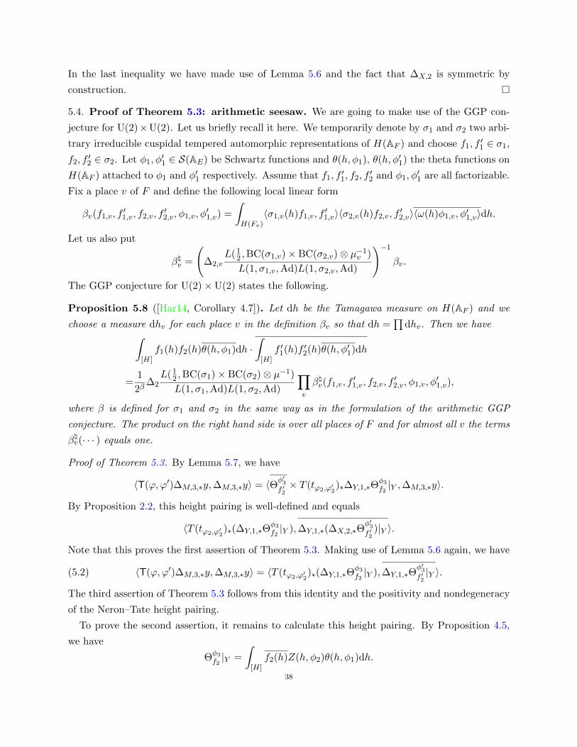
In the last inequality we have made use of Lemma 5.6 and the fact that ∆X,2 is symmetric by

construction.

5.4. Proof of Theorem 5.3: arithmetic seesaw. We are going to make use of the GGP con-

jecture for U(2)×U(2). Let us briefly recall it here. We temporarily denote by σ1 and σ2 two arbi-

trary irreducible cuspidal tempered automorphic representations of H(AF ) and choose f1, f′1 ∈ σ1,

f2, f′2 ∈ σ2. Let φ1, φ

′1 ∈ S(AE) be Schwartz functions and θ(h, φ1), θ(h, φ′1) the theta functions on

H(AF ) attached to φ1 and φ′1 respectively. Assume that f1, f′1, f2, f

′2 and φ1, φ

′1 are all factorizable.

Fix a place v of F and define the following local linear form

βv(f1,v, f′1,v, f2,v, f

′2,v, φ1,v, φ

′1,v) =

∫H(Fv)

〈σ1,v(h)f1,v, f′1,v〉〈σ2,v(h)f2,v, f

′2,v〉〈ω(h)φ1,v, φ′1,v〉dh.

Let us also put

β\v =

(∆2,v

L(12 ,BC(σ1,v)× BC(σ2,v)⊗ µ−1

v )

L(1, σ1,v,Ad)L(1, σ2,v,Ad)

)−1

βv.

The GGP conjecture for U(2)×U(2) states the following.

Proposition 5.8 ([Har14, Corollary 4.7]). Let dh be the Tamagawa measure on H(AF ) and we

choose a measure dhv for each place v in the definition βv so that dh =∏

dhv. Then we have∫[H]

f1(h)f2(h)θ(h, φ1)dh ·∫

[H]f ′1(h)f ′2(h)θ(h, φ′1)dh

=1

2β∆2

L(12 ,BC(σ1)× BC(σ2)⊗ µ−1)

L(1, σ1,Ad)L(1, σ2,Ad)

∏v

β\v(f1,v, f′1,v, f2,v, f

′2,v, φ1,v, φ

′1,v),

where β is defined for σ1 and σ2 in the same way as in the formulation of the arithmetic GGP

conjecture. The product on the right hand side is over all places of F and for almost all v the terms

β\v(· · · ) equals one.

Proof of Theorem 5.3. By Lemma 5.7, we have

〈T(ϕ,ϕ′)∆M,3,∗y,∆M,3,∗y〉 = 〈Θφ′3f ′2× T (tϕ2,ϕ′2

)∗∆Y,1,∗Θφ3f2|Y ,∆M,3,∗y〉.

By Proposition 2.2, this height pairing is well-defined and equals

〈T (tϕ2,ϕ′2)∗(∆Y,1,∗Θ

φ3f2|Y ),∆Y,1,∗(∆X,2,∗Θ

φ′3f ′2

)|Y 〉.

Note that this proves the first assertion of Theorem 5.3. Making use of Lemma 5.6 again, we have

(5.2) 〈T(ϕ,ϕ′)∆M,3,∗y,∆M,3,∗y〉 = 〈T (tϕ2,ϕ′2)∗(∆Y,1,∗Θ

φ3f2|Y ),∆Y,1,∗Θ

φ′3f ′2|Y 〉.

The third assertion of Theorem 5.3 follows from this identity and the positivity and nondegeneracy

of the Neron–Tate height pairing.

To prove the second assertion, it remains to calculate this height pairing. By Proposition 4.5,

we have

Θφ3f2|Y =

∫[H]

f2(h)Z(h, φ2)θ(h, φ1)dh.

38

Similarly for Θφ′3f ′2

. Therefore

(5.3)

〈T (tϕ2,ϕ′2)∗(∆Y,1,∗Θ

φ3f2

)|Y ,∆Y,1,∗Θφ′3f ′2|Y 〉

=

∫∫[H]2

f2(h)f ′2(h′)〈T (tϕ2,ϕ′2)∗∆Y,1,∗Z(h, φ2),∆Y,1,∗Z(h′, φ2)〉θ(h, φ1)θ(h′, φ′1)dhdh′.

This is the “arithmetic seesaw” alluded in the title of this subsection. Classically, the seesaw

argument amounts to changing order of integrations. In the current situation, the “arithmetic

seesaw” is changing the order of integration and the height pairing. The seesaw diagram we use

here is a “doubled” version of the following one

H(AF )×H(AF ) U(V)

H(AF ) U(W)×U(AE),

and the right hand side corresponds to the arithmetic intersection. Thus a diagram was first used

in [GGP12, Section 14] and then used in [Har14, Xue16] to relate the GGP conjecture (not the

arithmetic one) for U(n)×U(n+ 1) and for U(n)×U(n).

We make use of Proposition 5.8 to calculate the integral (5.3). We first note that since π3 and

π2 are both tempered, σ1 and σ2 are also tempered. Moreover, by looking at the archimedean

components of σ1 and σ2, cf. Lemma 3.1, we see that they do not come from theta lifts of unitary

groups of smaller size. Thus both σ1 and σ2 are stable, i.e. the base change of σ1 and σ2 are

cuspidal. Therefore when the GGP conjecture is applied to σ1 and σ2, we have β = 2. Combining

the GGP conjecture and Proposition 4.8, we obtain that

(5.3) =

(∆2

4

L(12 ,BC(σ1)× BC(σ2)⊗ µ−1)

L(1, σ1,Ad)L(1, σ2,Ad)

)×

((volK vol′K)−1 ×

L′(12 , σ1 × µ2)

L(1, η)ζ(2)

)

×∏v

(∆2,v

L(12 ,BC(σ1,v)× BC(σ2,v)⊗ µ−1

v )

L(1, σ1,v,Ad)L(1, σ2,v,Ad)

)−1

∫H(Fv)

〈σ2(h)f2,v, f ′2,v〉Z\v(ϕ2,v, ϕ

′2,v, ω(h)φ2,v, φ

′2,v)〈ωv(h)φ1, φ

′1〉dh.

Note that we have φ3,v = φ2,v ⊗ φ1,v, φ′3,v = φ′2,v ⊗ φ′1,v and 〈ϕ3,v, ϕ

′3,v〉 = Z\v(f2,v, f

′2,v, φ3,v, φ

′3,v).

With these choices, we have proved in [Xue16, Appendix A] that the double integral in the product

is absolutely convergent and equals α\v(ϕ3,v, ϕ′3,v, ϕ2,v, ϕ

′2,v). This is referred to as the local seesaw

identity in [Xue16]. Therefore by the identity (5.3), we conclude that

volK vol′K × 〈(T(ϕ,ϕ′)K′∆MK′ ,3,∗yK ,∆MK′ ,3,∗yK〉BB

=

(∆2

4

L(12 ,BC(σ1)× BC(σ2)⊗ µ−1)

L(1, σ1,Ad)L(1, σ2,Ad)

)(L′(1

2 , σ1 × µ2)

L(1, η)ζ(2)

)∏v

α\v(ϕ3,v, ϕ′3,v, ϕ2,v, ϕ

′2,v).

39

It is clear that the right hand side depends only on ϕ,ϕ′, but not on the choices of f2, f′2, φ3, φ

′3

and tϕ2,ϕ′2. This proves the second assertion of Theorem 5.3.

Appendix A. The Gross–Zagier formula

The goal of this appendix is to deduce Conjecture 5.1 in the case of n = 1 from the Gross–Zagier

formula in the generality of [YZZ13]. For simplicity, we do this only in a special case, namely,

F 6= Q so that the Shimura curve is proper, π2 is an automorphic representation of U(2)(AF ) with

trivial central character and π1 is the trivial representation of U(1)(AF ).

A.1. Formulae on quaternion algebras. Let us recall the results from [YZZ13] in this subsec-

tion. Due to the lack of space, we would not be able to explain all the definitions. The readers

should consult [YZZ13] for a detailed discussion. Let B be an incoherent quaternion algebra over

AF which ramifies at all archimedean places, i.e. B = ⊗vBv where Bv is a quaternion algebra of

Fv such that Bv is the Hamiltonian division algebra over R if v is archimedean and B is not of the

form B ⊗AF where B is a quaternion algebra over F . Attached to this B× is a (projective system

of) Shimura curve(s) defined over F , denoted by ShB× . We fix an embedding AE → B. The group

A×E acts on ShB× by the right translation. Let ShE×

B× be the subscheme fixed by E× (again defined

over F ) and P ∈ ShE×

B× (Eab) where Eab stands for the maximal abelian extension of E. Let ξP to

be the normalized Hodge bundle (cf. [YZZ13, p. 65]). We put

P =1

vol(E×\A×E/A×F )

∫E×\A×E/A

×F

Tt(P − ξP )dt ∈ Alb(ShB×)(F ),

where Tt is the Hecke operator defined by the “right multiplication by t” (cf. [YZZ13, p. 62], our

notation in Subsection 4.2 is γt). This is independent of the measure dt on A×E/A×F .

Let π be an irreducible admissible automorphic representation of B× appearing in H1(ShB×)

(this is called the automorphic representation of B× of weight zero in [YZZ13, Section 3.2.2]). We

assume that the central character of π is trivial. Note that π∞ is the trivial representation. Let

ϕ,ϕ′ ∈ π. A projector

T (ϕ⊗ ϕ′) : Alb(ShB×)→ Jac(ShB×).

is defined in [YZZ13, Subsection 3.3.1]. We briefly explain it here as follows. Fix an embedding

ι : F → C and an open compact subgroup K of B×(AF,f ). Fix an embedding ι : F → C. We have

H1,0(ShB×,ι,K(C)) ' ⊕σσK where σ stands for all the irreducible admissible representations of B×

which appears in the cohomology of ShB× . In particular any such a σ can be realized as a subspace

of H1,0(ShB×,ι(C)). We fix a pairing on H1,0(ShB×,ι(C)). Let ϕ,ϕ′ ∈ H1,0(ShB×,ιK(C)). Then put

〈ϕ,ϕ′〉 = (vol ShB×,ι,K(C))−1

∫ShB×,ι,K(C)

ϕ ∧ ϕ′.

40

This is independent of the choice of K and Hecke invariant. It thus gives an inner product on σ

and identifies σ with σ. There is an embedding⊕σK ⊗ σK → Hom(H1,0(ShB×,ι,K(C)),H1,0(ShB×,ι,K(C))),

and it is explained in [YZZ13, Proposition 3.14] that this embedding factors through the natural

map

Hom(Alb(ShB×,ι,K), Jac(ShB×,ι,K))→ Hom(H1,0(ShB×,ι,K(C)),H1,0(ShB×,ι,K(C))).

This defines the projector T (ϕ ⊗ ϕ′)K . As K varies, the system vol ShB×,ι,K(C) · T (ϕ ⊗ ϕ′)K is

independent of K. This is the projector T (ϕ⊗ ϕ′). The main result of [YZZ13] is the following.

Theorem A.1. We have

(A.1) 〈T (ϕ⊗ ϕ′)P , P 〉NT =ζF (2)L′(1

2 , πE)

4L(1, η)2L(1, π,Ad)

∏v

α\v(ϕv, ϕ′v).

The notation needs explanation.

– The height pairing is between Jac(ShB×)(F ) and Alb(ShB×)(F ). For any x ∈ Jac(ShB×)(L)

and y ∈ Alb(ShB×)(L), where L is a finite extension of F , we have the usual Neron–Tate

height pairing 〈x, y〉NT and the height pairing in the theorem is given by (L : F )−1〈x, y〉NT.

It has the property that it is independent of the field L in which x and y lie.

– The representation πE is the base change of π to GL2(AE). The adjoint L-function is the

one for π as a representation of PB× = B×/A×F . It is of degree three.

– The local linear form α\v is defined by

L(1, ηv)L(1, πv,Ad)

ζFv(2)L(12 , πv,Ev)

∫E×v /F

×v

〈πv(t)ϕv, ϕ′v〉dt

where the measure dtv is specified in [YZZ13, Subsection 1.6]. What we need about these

measures is that the product∏v dtv is not the Tamagawa measure of A×E/A

×F , but rather

the one that gives vol(E×\A×E/A×F ) = 2L(1, η).

For our purposes, we need such a formula for the Shimura curves attached to PB×. We have

a Shimura curve ShPB× defined over F , and a morphism p : ShB× → ShPB× . The embedding

A× → B× induces an embedding A×E/A×F → PB×. The group A×E/A

×F acts on ShPB× by right

translation. We let P ′ = p(P ) ∈ ShE×/F×

PB× (Eab). We define

P ′ =1

vol(E×\A×E/A×F )

∫E×\A×E/A

×F

Tt(P′ − ξP ′)dt ∈ Alb(ShPB×)(F ),

where Tt is again the “right multiplication by t”. It is clear that p∗(P ) = P ′.

The representation π is naturally a representation of PB×. Thus for ϕ,ϕ′ ∈ π, we may again

define a projector

S(ϕ⊗ ϕ′) : Alb(ShPB×)→ Jac(ShPB×).

Then we have41

Lemma A.2. We have

〈S(ϕ⊗ ϕ′)P ′, P ′〉NT =ζF (2)L′(1

2 , πE)

4L(1, η)2L(1, π,Ad)

∏v

α\v(ϕv, ϕ′v),

where the height pairing is defined in the same way as in Theorem A.1 and the right hand side is

the same as that of (A.1).

Proof. Since p∗P = P ′, by the projection formula, we only have to prove that

p∗S(ϕ⊗ ϕ′)p∗ = T (ϕ⊗ ϕ′).

This can be proved in the same way as [YZZ13, Proposition 3.14(2)]. We omit the details.

A.2. Unitary groups in two variables. The discussion in this subsection is a very special case

of [HS12, Chapter 4]. Due to the lack of space, we would not be able to explain all the details. The

readers should consult [HS12] for a detailed exposition.

In the following we denote by ν : B× → A×F the reduced norm of B. With the embedding AE → B,

the incoherent quaternion algebra B is a two dimensional incoherent Hermitian space over AE . It is

well-known that U(B) ' (B××A×E)1/A×F where the superscript 1 means that it consists of elements

(b, e) such that ν(b) = NE/F (e) and A×F embeds diagonally. We also have the similitude unitary

group GU(B) ' (B××A×E)/A×F and the similitude factor is given by (b, e) 7→ ν(b)NE/F (e)−1. Note

that the center of GU(B) isomorphic to A×E , embedded in GU(B) as (1, e), e ∈ A×E . We have

morphisms U(B) → GU(B) → PB× which is the natural inclusion followed by projecting to the

first factor. The image of this composition consists of elements whose reduced norm lie in NA×Ewhich we denote by PB×,†. We have a morphism ShU(B) → ShPB× whose image is ShPB×,† , the

Shimura variety attached to PB×,†.Recall that we have a representation π of PB×. Let us fix an embedding ι : F → C and an

embedding ι′ : E → C above it. Then π can be realized as a subrepresentation of H1,0(ShPB×,ι(C))

under the action of PB×. We fix this realization of π. We let π+ be the restriction of π to U(B)

along the morphism ShU(B),ι′(C)→ ShPB×,ι(C). Note that this is the restriction of the differential

forms, not the the restriction of the representation π to the group U(B). Then π+ is a subspace of

H1,0(ShU(B),ι′(C)).

We now relate our situation to that in [HS12, Chapter 4]. Let B(ι) be the nearby quaternion

algebra of B at ι, i.e. a quaternion algebra over F which differs from B only at the place ι. Let

π(ι) be the Jacquet–Langlands transfer of π to B(ι)(AF ). This is an automorphic representation

of B(ι)(AF ). We have π(ι)v ' πv if v 6= ι and π(ι)ι is the discrete series representation of B(ι)(Fι)

of weight two. Then π can be identified with a subspace of π(ι) consisting of automorphic forms

on B(ι)(AF ) that are holomorphic at the place ι, i.e. the ι component is a lowest weight vector.

In fact, there is a standard way to pass from a holomorphic differential form on ShPB×,ι(C) to

an automorphic form on B(ι)(AF ) which is holomorphic at ι. The most general discussion is

in [Har84, Section 2.1, 2.2]. But in our special situation, the usual passage “differential forms” →42

“modular forms” → “automorphic forms” suffices. With a similar discussion as above, one has an

automorphic representation π+(ι) of U(B(ι))(AF ) and π+ is can be identified with a subspace of

π+(ι) consisting of automorphic forms on U(B(ι))(AF ) that are holomorphic at the place ι. The

restriction of differential forms along the morphism ShU(B),ι′(C) → ShPB×,ι(C) corresponds to the

restriction of automorphic forms along the natural map U(B(ι))(AF ) → B(ι)(AF ). The relation

between π+ and π is thus transformed to that of π+(ι) and π(ι), the later being discussed in detail

in [HS12, Chapter 4]. In the notation there, G = U(B(ι)) and G = GU(B(ι)) = (B(ι)××E×)/F×,

and they have the same derived group.

We now explaining the relation between π+ and π. There are two cases.

(1) π ⊗ η ν 6' π. In this case, by [HS12, Theorem 4.14], the natural map π → π+ is a bi-

jection. Moreover all irreducible constituents of the restriction of π to U(B), as abstract

representations, are automorphic. By [HS12, Proposition 4.21], these constituents are mu-

tually inequivalent (as abstract representations). We denote by π0 one of the irreducible

constituent of π+. We have that πE (which is the same as BC(π0)) is a cuspidal automor-

phic representation of GL2(AE). As π0 is realized naturally on some subspace of π, we put

an inner product on π0 by restricting that from π. Thus suppose we have ϕ,ϕ′ ∈ π and

ϕ0, ϕ′0 their restrictions to ShU(B),ι′ , then 〈ϕ,ϕ′〉π = 〈ϕ0, ϕ′0〉π0 .

Now suppose that π = ⊗πv. Then π0 = ⊗π0v where π0

v is an irreducible constituent

of πv, as an abstract representation of U(B)(Fv). Note that by [HS12, Lemma 2.4, 2.12],

πv is irreducible (resp. direct sum of two inequivalent irreducible representations) if πv ⊗ηv νv 6' πv (resp. '). Let us fix an inner product 〈−,−〉πv on πv for each v so that

〈−,−〉π =∏v〈−,−〉πv . By restricting the inner product on πv to its irreducible constituents,

we obtain an inner product on each π0v . We then have 〈−,−〉π0 =

∏v〈−,−〉π0

v.

(2) π ⊗ η ν ' π. Then for places v, πv ⊗ ηv νv ' πv we have πv = π+v ⊕ π−v where π±v

is an irreducible representation of U(B)(Fv) (if v is archimedean, then we put π−v = 0).

We choose the labeling so that if πv is an unramified representation of PB×(Fv), then

π+v is an unramified representation of U(B)(Fv). We may moreover assume that ⊗π+

v

is an irreducible constituent of π0, i.e. it is automorphic as a representation of U(B).

By [HS12, Proposition 4.21], we have that ⊗πεvv where εv = ± is automorphic if and only if

there are even number of minus signs in εv, in other words,

π+ '⊕

∏v εv=1

⊗πεvv .

Let π1 (resp. π2) be the subspace of π consisting of ϕ’s that are (resp. are not) supported

in the image of ShU(B),ι′(C) in ShPB×,ι(C). Then by [HS12, Lemma 4.14, Theorem 4.14],

π1 and π2 are representations of U(B), the natural restriction map π → π+ (restriction as

functions) identifies π1 with π+ as U(B) representations and the kernel is π2.43

Let π0 = ⊗πεvv be an irreducible constituent of π+. Since π1 → π+ is an isomorphism,

we see that π0 is again naturally realized on a subspace of π. Thus we may define inner

products on π0 and π0v as in the previous case, i.e. by restricting inner products from π and

πv respectively. In this way, we again have

〈ϕ,ϕ′〉π = 〈ϕ′0, ϕ′0〉π0 , 〈ϕ0, ϕ′0〉π0 =∏v

〈ϕ0v, ϕ′0v 〉,

where ϕ,ϕ′ ∈ π1 and ϕ0, ϕ′0 their restrictions to U(B) respectively.

A.3. The formula on the unitary groups. Let us get back to the setup of Conjecture 5.1 in

the case of n = 1. Recall that we have put G = U(B) × U(AE) and H = U(AE). We have the

Shimura curve M attached to G defined over E. The group H embeds in G diagonally and acts by

right translation on M . Let K ′ be an open compact subgroup of G(AF,f ) and K = K ′ ∩H(AF,f ).

Then we put

QK′ = (#YK)−1yK,0 ∈ Alb(MK′)(E),

where yK,0 = ∆MK′ ,1,∗yK and the ∆MK′ ,1 is the first Kunneth–Chow component of MK′ defined

using the Hodge bundle. As K varies, we have a system Q ∈ Alb(M)(E).

We have a representation π of PB× (with the realization discussed in the previous subsection)

and its restriction to U(B) (the restriction of differential forms as discussed before). We let π0

be an irreducible constituent of this restriction. By extending it trivially on A×E , we view π0 as a

representation of G.

If π⊗ην 6' π (resp. '), we put π1 = π (resp. π1 as in the previous subsection). Let ϕ0, ϕ′0 ∈ π0

and choose ϕ,ϕ′ ∈ π1 so that their restrictions are ϕ0 and ϕ′0 respectively. Similarly to the case of

Shimura varieties attached to quaternion algebras, we have a projector R(ϕ0 ⊗ ϕ′0).

Lemma A.3. We have

〈R(ϕ0 ⊗ ϕ′0)Q,Q〉NT =ζF (2)L′(1

2 , πE)

2sL(1, η)L(1, π0,Ad)

∏v

α\v(ϕv, ϕ′v),

where s = 2 or 1 according to whether π⊗ (η ν) ' π or not, the local linear forms α\v on the right

hand side are the same as that of (A.1), the adjoint L-function is the adjoint L-function for π0

as a representation of U(B), and the height pairing is the usual height pairing between Alb(M)(E)

and Jac(M)(E).

Proof. Let us denote by p : M → ShPB× the natural morphism. We fix a an embedding ι : F → Cand an embedding ι′ : E → C over it. Choose open compact subgroups K of PB×(AF,f ) and K ′

of G(AF,f ) which maps into K. The morphism p induces the natural morphisms p∗ and p∗ on the

level of differential forms. The map p∗ is simply the pullback map while p∗ is more complicated.

If f ∈ H1,0(ShPB×,ι,K(C)), then we have p∗p∗f = deg p · f ′ where deg p stands for the degree of the

44

morphism from Mι′,K′(C) to its image in ShPB×,ι,K(C) and f ′ stands for the restriction of f to the

image of p. We claim that

R(ϕ0 ⊗ ϕ′0) = 2s−1p∗T (ϕ⊗ ϕ′)p∗.

Assume this for the moment, we see that Lemma A.3 follows from Lemma A.2. This is because of

p∗Q = P ′ ∈ ShPB×(F ) and the projection formula. We only need to note that the height pairing

in Lemma A.2 is over F while it is over E in Lemma A.3. Moreover we have L(1, π0,Ad) =

L(1, η)L(1, π,Ad).

It remains to prove the claim. We only have to prove it in Hom(H1,0(Mι(C)),H1,0(Mι(C))). Let

f0 ∈ π0 and choose an element f ∈ π1 whose restriction is f0. We have

R(ϕ0 ⊗ ϕ′0)f0 = vol ShU(B),ι′,K′(C) · 〈f, ϕ′〉ϕ0,

and

p∗T (ϕ⊗ ϕ′)p∗f0 = vol ShPB×,ι,K(C) · 〈p∗p∗f, ϕ′〉ϕ0.

Here the pairings are the ones on H1,0(ShPB×,ι,K(C)). The point is that p∗p∗f is not simply a

multiple of f in the case π ⊗ η ν 6' π. Indeed, if π ⊗ η ν ' π, then p∗p∗f = deg p · f , Thus

〈p∗p∗f, ϕ′〉 = 〈f, ϕ′〉. If π ⊗ η ν 6' π, we however have

2〈p∗p∗f, ϕ′〉 = deg p · 〈f, ϕ′〉.

We also have 2 vol ShU(B),ι′,K′(C) = deg p · vol ShPB×,ι,K(C). The claim then follows.

With all these preparations, we can now prove the following result.

Proposition A.4. Let K ′ be an open compact subgroup of G(AF,f ). We keep the notation in

Conjecture 5.1. Then we have

(volK)2(volMK′ vol′K ′)〈T (tϕ0,ϕ′0)K′,∗yK,0, yK,0〉NT =ζF (2)L′(1

2 , πE)

2sL(1, π0,Ad)

∏v

α\v(ϕ0v, ϕ′0v ),

where the height pairing is between Alb(MK′)(E) and Jac(MK′)(E), the adjoint L-function on the

right hand side is the adjoint L-function of π as a representation of U(B), s = 2 or 1 according to

whether π ⊗ (η ν) ' π or not. Under our choice of the measures we have volK#YK = 1.

Remark A.5. In terms of the notation in Conjecture 5.1, β = s + 1. Moreover πE = BC(π0). In

particular, Conjecture 5.1 holds in this case.

Proof. Let us first explain that the projector can be alternatively defined in terms of the Hecke

operators as follows. Let K ′ be an open compact subgroup of G(AF,f ). Fix a measure on G(AF,f )

and denote the volume of any open compact by vol′. Then as in Subsection 4.2, we have a Hecke

correspondence T (tϕ0,ϕ′0)K′ on MK′ ×MK′ . It defines a map

T (tϕ0,ϕ′0)K′,∗ : Alb(MK′)→ Jac(MK′).45

As K ′ varies, the system vol′K ′ volMK′T (tϕ0,ϕ′0)K′,∗ defines a map Alb(M) → Jac(M), which

is the desired projector R(ϕ0 ⊗ ϕ′0) (cf. [YZZ13, Proposition 3.14]).

Let us choose ϕ,ϕ′ ∈ π1 so that there restriction to π0 is ϕ0 and ϕ′0 respectively. By the above

explanation of the projectors in terms of the Hecke operators, the left hand side equals

(volK#YK)2〈R(ϕ0 ⊗ ϕ′0)Q,Q〉NT.

By Lemma A.3, this equals

(volK#YK)2 ζF (2)L′(12 , πE)

2sL(1, η)L(1, π,Ad)

∏v

α\v(ϕv, ϕ′v).

In Conjecture 5.1, the product of the measures in defining α\v is the Tamagawa measure of A×E/A×F

while the product of the measures in defining α\v is L(1, η) times the Tamagawa measure. It follows

that the left hand side equals

(volK#YK)2 ζF (2)L′(12 , πE)

2sL(1, π,Ad)

∏v

α\v(ϕ0v, ϕ′0v ).

It remains to prove that volK#YK = 1 when K is small. Note that E×/F× is discrete in

A×E,f/A×F,f . It follows from the definition of YK that

volK#YK = volE×\A×E,f/A×F,f .

Moreover under the normalized local measure, we have volC×/R× = 1. Therefore we have

volE×\A×E,f/A×F,f = volE×\A×E/A

×F ,

where the vol on the right hand side is computed using the product the normalized local measures

divided by 2L(1, η). The product of normalized local measures (over all places) is L(1, η) times the

Tamagawa measure of A×E/A×F . Thus we have volE×\A×E/A

×F = 1 and hence volK#YK = 1. This

proves the proposition.

References

[BP] R. Beuzart-Plessis, A local trace formula for the GGP conjecture for unitary groups: the archimedean case.

To appear in Asterisque. ↑19, 20, 21, 22

[BWR15] J. H. Bruinier and M. Westerholt-Raum, Kudla’s modularity conjecture and formal Fourier-Jacobi series,

Forum Math. Pi 3 (2015), e7, 30. MR3406827 ↑26, 27

[GGP12] W. T. Gan, B. H. Gross, and D. Prasad, Symplectic local root numbers, central critical L values, and

restriction problems in the representation theory of classical groups, Asterisque 346 (2012), 1–109 (English,

with English and French summaries). Sur les conjectures de Gross et Prasad. I. MR3202556 ↑2, 32, 39

[GI14] W. T. Gan and A. Ichino, Formal degrees and local theta correspondence, Invent. Math. 195 (2014), no. 3,

509–672, DOI 10.1007/s00222-013-0460-5. MR3166215 ↑20

[GI16] , The Gross-Prasad conjecture and local theta correspondence, Invent. Math. 206 (2016), no. 3,

705–799, DOI 10.1007/s00222-016-0662-8. MR3573972 ↑20

[GT16] W. T. Gan and S. Takeda, A proof of the Howe duality conjecture, J. Amer. Math. Soc. 29 (2016), no. 2,

473–493, DOI 10.1090/jams/839. MR3454380 ↑16

46

[Gro04] B. H. Gross, Heegner points and representation theory, Heegner points and Rankin L-series,

Math. Sci. Res. Inst. Publ., vol. 49, Cambridge Univ. Press, Cambridge, 2004, pp. 37–65, DOI

10.1017/CBO9780511756375.005. MR2083210 ↑2[GP92] B. H. Gross and D. Prasad, On the decomposition of a representation of SOn when restricted to SOn−1,

Canad. J. Math. 44 (1992), no. 5, 974–1002, DOI 10.4153/CJM-1992-060-8. MR1186476 ↑2[GS95] B. H. Gross and C. Schoen, The modified diagonal cycle on the triple product of a pointed curve, Ann. Inst.

Fourier (Grenoble) 45 (1995), no. 3, 649–679 (English, with English and French summaries). MR1340948

↑36

[GZ86] B. H. Gross and D. B. Zagier, Heegner points and derivatives of L-series, Invent. Math. 84 (1986), no. 2,

225–320, DOI 10.1007/BF01388809. MR833192 ↑2[Har84] M. Harris, Eisenstein series on Shimura varieties, Ann. of Math. (2) 119 (1984), no. 1, 59–94, DOI

10.2307/2006963. MR736560 ↑42

[Har07] , Cohomological automorphic forms on unitary groups. II. Period relations and values of L-functions,

Harmonic analysis, group representations, automorphic forms and invariant theory, Lect. Notes Ser.

Inst. Math. Sci. Natl. Univ. Singap., vol. 12, World Sci. Publ., Hackensack, NJ, 2007, pp. 89–149, DOI

10.1142/9789812770790 0005. MR2401812 ↑17

[HKS96] M. Harris, S. S. Kudla, and W. J. Sweet, Theta dichotomy for unitary groups, J. Amer. Math. Soc. 9

(1996), no. 4, 941–1004, DOI 10.1090/S0894-0347-96-00198-1. MR1327161 ↑18

[Har14] R. N. Harris, The refined Gross-Prasad conjecture for unitary groups, Int. Math. Res. Not. IMRN 2 (2014),

303–389. MR3159075 ↑3, 38, 39

[HS12] K. Hiraga and H. Saito, On L-packets for inner forms of SLn, Mem. Amer. Math. Soc. 215 (2012), no. 1013,

vi+97, DOI 10.1090/S0065-9266-2011-00642-8. MR2918491 ↑42, 43

[How89] R. Howe, Transcending classical invariant theory, J. Amer. Math. Soc. 2 (1989), no. 3, 535–552, DOI

10.2307/1990942. MR985172 ↑16

[II10] A. Ichino and T. Ikeda, On the periods of automorphic forms on special orthogonal groups and the Gross-

Prasad conjecture, Geom. Funct. Anal. 19 (2010), no. 5, 1378–1425, DOI 10.1007/s00039-009-0040-4.

MR2585578 (2011a:11100) ↑3, 5

[KMSW] T. Kaletha, A. Minguez, S.-W. Shin, and P.-J. White, Endoscopic Classification of Representations: Inner

Forms of Unitary Groups, available at https://arxiv.org/abs/1409.3731. ↑31

[Kud97] S. S. Kudla, Algebraic cycles on Shimura varieties of orthogonal type, Duke Math. J. 86 (1997), no. 1,

39–78, DOI 10.1215/S0012-7094-97-08602-6. MR1427845 ↑26

[Kud04] , Special cycles and derivatives of Eisenstein series, Heegner points and Rankin L-series,

Math. Sci. Res. Inst. Publ., vol. 49, Cambridge Univ. Press, Cambridge, 2004, pp. 243–270, DOI

10.1017/CBO9780511756375.009. MR2083214 ↑2[KRY06] S. S. Kudla, M. Rapoport, and T. Yang, Modular forms and special cycles on Shimura curves, Annals of

Mathematics Studies, vol. 161, Princeton University Press, Princeton, NJ, 2006. MR2220359 ↑5[KM90] S. S. Kudla and J. J. Millson, Intersection numbers of cycles on locally symmetric spaces and Fourier

coefficients of holomorphic modular forms in several complex variables, Inst. Hautes Etudes Sci. Publ.

Math. 71 (1990), 121–172. MR1079646 ↑23, 26, 28

[LR05] E. M. Lapid and S. Rallis, On the local factors of representations of classical groups, Automorphic repre-

sentations, L-functions and applications: progress and prospects, Ohio State Univ. Math. Res. Inst. Publ.,

vol. 11, de Gruyter, Berlin, 2005, pp. 309–359, DOI 10.1515/9783110892703.309. MR2192828 ↑18

[Li92] J.-S. Li, Nonvanishing theorems for the cohomology of certain arithmetic quotients, J. Reine Angew. Math.

428 (1992), 177–217, DOI 10.1515/crll.1992.428.177. MR1166512 ↑18

47

[LST11] J.-S. Li, B. Sun, and Y. Tian, The multiplicity one conjecture for local theta correspondences, Invent. Math.

184 (2011), no. 1, 117–124, DOI 10.1007/s00222-010-0287-2. MR2782253 ↑16

[Liu11a] Y. Liu, Arithmetic theta lifting and L-derivatives for unitary groups, I, Algebra Number Theory 5 (2011),

no. 7, 849–921. MR2928563 ↑2, 6, 8, 9, 23, 24, 25, 26, 28

[Liu11b] , Arithmetic theta lifting and L-derivatives for unitary groups, II, Algebra Number Theory 5 (2011),

no. 7, 923–1000. MR2928564 ↑2, 7, 8, 28

[Liu12] , Arithmetic inner product formula for unitary groups, ProQuest LLC, Ann Arbor, MI, 2012. Thesis

(Ph.D.)–Columbia University. MR3029684 ↑9[Mok15] C. P. Mok, Endoscopic classification of representations of quasi-split unitary groups, Mem. Amer. Math.

Soc. 235 (2015), no. 1108, vi+248, DOI 10.1090/memo/1108. MR3338302 ↑31

[Pau98] A. Paul, Howe correspondence for real unitary groups, J. Funct. Anal. 159 (1998), no. 2, 384–431, DOI

10.1006/jfan.1998.3330. MR1658091 ↑17

[RSZ] M. Rapoport, B. Smithling, and W. Zhang, On the arithmetic transfer conjecture for exotic smooth formal

moduli spaces. To appear in Duke Math Journal. ↑5[SZ07] P. Schneider and E.-W. Zink, The algebraic theory of tempered representations of p-adic groups. I. Parabolic

induction and restriction, J. Inst. Math. Jussieu 6 (2007), no. 4, 639–688, DOI 10.1017/S1474748007000047.

MR2337311 ↑22

[Wal90] J.-L. Waldspurger, Demonstration d’une conjecture de dualite de Howe dans le cas p-adique, p 6= 2,

Festschrift in honor of I. I. Piatetski-Shapiro on the occasion of his sixtieth birthday, Part I (Ramat Aviv,

1989), Israel Math. Conf. Proc., vol. 2, Weizmann, Jerusalem, 1990, pp. 267–324 (French). MR1159105

↑16

[Xue16] H. Xue, Fourier-Jacobi periods and the central value of Rankin-Selberg L-functions, Israel J. Math. 212

(2016), no. 2, 547–633, DOI 10.1007/s11856-016-1300-2. MR3505397 ↑7, 39

[Xue] , On the global GGP conjecture for unitary groups: approximating smooth transfer of Jacquet–Rallis.

preprint. ↑5[YZZ09] X. Yuan, S.-W. Zhang, and W. Zhang, The Gross-Kohnen-Zagier theorem over totally real fields, Compos.

Math. 145 (2009), no. 5, 1147–1162, DOI 10.1112/S0010437X08003734. MR2551992 ↑6, 27

[YZZ13] , The Gross-Zagier formula on Shimura curves, Annals of Mathematics Studies, vol. 184, Princeton

University Press, Princeton, NJ, 2013. MR3237437 ↑2, 3, 8, 34, 40, 41, 42, 46

[YZZ] , Triple product L-series and Gross–Kudla–Schoen cycles, available at https://www.math.

columbia.edu/~wzhang/math/online/triple.pdf. preprint. ↑5[Zha10] S.-W. Zhang, Gross-Schoen cycles and dualising sheaves, Invent. Math. 179 (2010), no. 1, 1–73, DOI

10.1007/s00222-009-0209-3. MR2563759 ↑11, 12

[Zha] , Linear forms, algebraic cycles, and derivatives of L-series. Preprint. ↑32

[Zha12] W. Zhang, On arithmetic fundamental lemmas, Invent. Math. 188 (2012), no. 1, 197–252, DOI

10.1007/s00222-011-0348-1. MR2897697 ↑2, 5, 32

[Zha14a] , Automorphic period and the central value of Rankin-Selberg L-function, J. Amer. Math. Soc. 27

(2014), no. 2, 541–612, DOI 10.1090/S0894-0347-2014-00784-0. MR3164988 ↑33

[Zha14b] , Fourier transform and the global Gan-Gross-Prasad conjecture for unitary groups, Ann. of Math.

(2) 180 (2014), no. 3, 971–1049. MR3245011 ↑5[Zha] , Relative trace formula and arithmetic GGP conjecture. preprint. ↑10, 32

Department of Mathematics, The University of Arizona. 617 N. Santa Rita Ave. Tucson, AZ 85721

E-mail address: xuehang@math.arizona.edu

48