Ariadna Study: Space Gaits - esa.int Study Report/ACT-RPT-AI-ARI-12-52… · Ariadna Study: Space...

1/48

Ariadna Study: Space Gaits

Final Report Authors: Evangelos G. Papadopoulos, Senior Researcher Ioannis Kontolatis, Junior Researcher Iosif S. Paraskevas, Junior Researcher Affiliation: Control Systems Laboratory Department of Mechanical Engineering National Technical University of Athens (NTUA) Heroon Polytechniou 9, 15780 Zografou, Athens, GREECE Date: 28 June 2013

ACT research category: Artificial Intelligence Contacts: Evangelos G. Papadopoulos Tel: +30-210-772-1440 Fax: +30-210-772-1455 e-mail: [email protected]

Leopold Summerer (Technical Officer) Tel: +31(0)715654192 Fax: +31(0)715658018 e-mail: [email protected]

Available on the ACT website

http://www.esa.int/act

Ariadna ID: 12/5201 Ariadna study type: Standard

Contract Number: 4000105989/12/NL/KML

2/43

Abstract

Locomotion using legs offers a great potential to mobile platforms transversing unstructured environments in terms of speed, energy efficiency and adaptation. Planets, satellites, and asteroids, presenting great scientific and exploration interest, are all characterized by such environments and therefore are candidate to be explored by legged locomotion platforms. Although research in legged robots over the last three decades led to several models, control algorithms and designs, a general systematic approach to the design and selection of appropriate gaits is lacking.

This study examines the effects of gravity, slopes, and stiffness to the gaits achieved by quadruped robots in dynamic walking and running. To this aim, Hildebrand gait diagrams are employed in analysing gaits resulting from an optimisation process according to criteria important for space missions, such as motion speed and energy efficiency. A lumped parameter model of a quadruped robot in the sagittal and the coronal plane, is obtained using the Lagrangian methodology, and used in a simulation set-up to tackle the body pitch/ roll stabilization problem. Appropriate models for the environment including gravity and soil properties are used. An optimization study based on an extensive analysis using numerical return maps and passive robot models is used to determine the conditions required for achieving steady state cyclic motion. The results are evaluated using an appropriate objective function, an optimization algorithm and a complex quadruped robot model. The optimum gaits are classified using an automated scheme based on the Hildebrand gait diagrams.

This study showed that it is possible to obtain stable gaits despite the varied conditions encountered in planetary exploration, and therefore, it indicates that legged robots can be used in such missions. It also presents important design guidelines that can be useful in designing robots able to complete their exploratory tasks successfully.

3/48

TABLE OF CONTENTS

ABSTRACT 2

TABLE OF CONTENTS 3

1. INTRODUCTION 5 1.1 CONCEPT 5 1.2 MOTIVATION 5 1.3 LITERATURE SURVEY 6 1.4 CONTENTS OF THIS WORK 7

2 ROBOT DYNAMICS 8 2.1 CONCEPT 8 2.2 MOTIVATION 8 2.3 LITERATURE SURVEY 8 2.4 CONTENTS OF THIS WORK 9

3 ENVIRONMENTAL CONDITIONS 12 3.1 GRAVITY 12 3.2 TOPOGRAPHIC FEATURES 13 3.3 SURFACE CHARACTERISTICS 14 3.4 SUBSURFACE CHARACTERISTICS 15

3.4.1 PROBLEM STATEMENT 15 3.4.2 MODELLING OF INTERACTION WITH SOIL 17 3.4.3 IMPACT DYNAMICS BETWEEN SOIL AND LEG 18 3.4.4 FRICTION AND TANGENTIAL EFFECTS 25 3.4.5 EQUIVALENT STIFFNESS AND DAMPING 25

3.5 COMPUTER PROGRAMS FOR ENVIRONMENTAL PARAMETERS 26 3.5.1 GROUND PARAMETERS 26 3.5.2 INTERACTIVE PROGRAM 26 3.5.3 PROGRAM FOR BATCH FILES CREATION 26 3.5.4 CONTACT INTERACTION 27

4 GAIT CLASSIFICATION 28 4.1 CONCEPT 28 4.2 MOTIVATION 28 4.3 LITERATURE SURVEY 28 4.4 CONTENTS OF THIS WORK 28

4.4.1 HILDEBRAND DIAGRAMS 28 4.4.2 RESULTS 30

4/48

5. OPTIMIZATION 37 5.1 CONCEPT 37 5.2 MOTIVATION 37 5.3 LITERATURE SURVEY 37 5.4 CONTENTS OF THIS WORK 37

5.4.1 EXTENSIVE SEARCH 37 5.4.2 MATHWORKS FMINCON 38 5.4.3 RESULTS 39

5.5 COMPUTER PROGRAMS FOR GAIT GRAPHS AND OPTIMIZATION 45

6 CONCLUSIONS 46

REFERENCES 47

5/48

1. Introduction

1.1 Concept Exploration missions of celestial bodies can benefit by employing legged robots. However, locomotion using legs, and especially dynamically stable locomotion, is highly depended on the local gravity field. On the other hand, exploration missions have specific requirements, such as low weight, radiation resilience, energy efficiency and system reliability. In addition, maintenance is impossible; therefore under critical situations a mission can be abruptly terminated. To this end, a systematic methodology is required for designing and implementing specific legged systems, according to the various challenging constraints of a space mission. An important ingredient of this approach is the study of the evolution of gait patterns as a function of gravity, and mission requirements such as transversal speed, environment morphology, power consumption, etc.

1.2 Motivation Humans and animals have incredible motion capabilities in terms of speed, energy efficiency and traversing capabilities of environments with rough terrain, extreme slopes, and obstacles, such as off-road and mountainous areas, earthquake ruins, volcanoes, etc. These capabilities are due mainly to their legged locomotion system that allows them to use discrete footprints to handle discontinuities. Also, they change the stiffness of their muscles and the distance between their CoM and the ground to preserve their desired motion in an efficient way despite ground inclination and obstacles. In addition, humans and animals are able to perform dynamically stable motions in order to achieve higher speeds.

Robotics researchers and scientists have been intrigued by these phenomenal characteristics since more than thirty years. The effort of mimicking nature led to a number of legged robot designs that can be classified as statically and dynamically stable. The development of legged robots with capabilities close to those of animals or humans opens new and exciting possibilities, such as reaching distant points through rough or slopped terrain, detecting survivors in earthquake ruins or workers in mine tunnels, helping in fire-fighting or de-mining tasks, or exploring planets.

The exploration of planets, satellites and asteroids is undoubtedly significant for mankind. Wheeled robots have already been used in space exploration, sometimes having faced formidable obstacles. Legged locomotion is a natural alternative that has great potentials. The transversal of rough terrain and the small footprint requirements can be met by the development and use of legged robots. Although legged machines have the potential to outperform wheeled vehicles on rough terrain, they are subject to complex motion control challenges and to balance-in-motion constraints. Simply controlling the forward speed becomes a much more involved issue than in wheeled vehicles.

6/48

1.3 Literature Survey Significant efforts have focused on legged robots due to their efficiency, particularly in uneven terrains, and their capability in sloping ground locomotion. A number of approaches aiming at using legged robots for celestial body exploration have been presented up to date. To name a few, researchers at the Jet Propulsion Laboratory proposed the All-Terrain Hex-Limbed Extra-Terrestrial Explorer (ATHLETE) concept as a mobility platform for lunar operations [1]. ATHLETE is a six limbed hybrid mobile platform designed to traverse quickly over smooth terrain using its wheels, traverse uneven terrain using its limbs and perform general manipulation of tools and payloads. Also, ATHLETE used as an evaluation testbed for a method of modelling compliance. This method assumes that all of the robot’s compliance takes place at the ground contact points, specifically the tires and legs, and that the rest of the robot is rigid [2]. The robots of the ATHLETE family use statically stable gaits, without capability of quick motions or right themselves from an unstable position. Therefore, predictive gait planning becomes very challenging and necessary. Another six-legged robot proposed for planetary exploration is the DLR Crawler [3]. It is an actively compliant walking robot that implements a walking layer with a simple tripod and a more complex biologically inspired gait. A navigation layer enables the robot to autonomously find a path to a predefined goal point. Nevertheless, the robot lacks a planner for footholds and body poses to handle highly uneven terrains.

A different concept of a steerable six-legged hopping robot proposed in [4]. The robot can be launched from a base lander or vehicle and retrieved using a tether mechanism. Although a simulation of a hopping robot was designed to study and test the hopping robot parameters for the launch and retrieval system in different gravitational environments, a systematic gait planning, e.g. for stability purposes, was not presented. Instead, an internal gyro was used to help stabilize the robot, allowing it to stay upright and land on its feet when hopping at angles. The ASTRO is a six-limbed ambulatory locomotion system that replicates walking gaits of the arachnid insects [5]. A microgravity emulation testbed for asteroid exploration robots was presented for validating control methods using the ASTRO in hardware-in-the-loop simulations [5]. As the researchers stated, the main purpose of this motion technique, is to avoid getting ejected from the surface of the asteroid. Nevertheless, motion patterns and landing strategies were not proposed.

Researchers from DFKI presented the concept of a biologically inspired, energy-efficient and adaptively free-climbing six-legged robot for steep slopes [6]. They focused on robot foot-design aiming at handling constraints from the environmental ground conditions, i.e. soft or steep terrain. They used a Central Pattern Generator (CPG) to generate the rhythmic walking motions and control the coordination for all legs. Although the prototype robot handles slopes around 25o while moving with a uniformly distributed walking gait or a tripod gait, its forward speed is quite slow, i.e. 125 mm/s, as expected for a statically stable gait. A quadruped concept design for planetary exploration is presented in [7]. The system was built for upright walking but its wide range of

7/48

motion in all joints allows switching to a turtle-like crawling gait when loose soil or steep slopes are encountered. Also, it is capable of recovery manoeuvres after tipping over. A comparison with a six-wheeled rover in terms of obstacle handling and static stability proved that the legged locomotion system is a worthy option for planetary exploration. In this case also, the robot uses statically stable gaits for the sake of stability, which reduces its speed capability.

1.4 Contents of this work This work presents a systematic study of legged locomotion gaits as a function of gravity and environmental morphology, employing Hildebrand gait diagrams. The gaits are the result of an optimisation process and are studied according to criteria important to space missions, such as motion speed, energy efficiency or range, and climbing capabilities.

8/48

2 Robot Dynamics

2.1 Concept Experimental evidence from research in Biology suggests that the high level nervous system is not required for steady state level walking and running, while research in Physiology indicates that during rapid locomotion, the control is dominated by the mechanical system. Similar results were presented from research in passive legged mechanisms that walk without the need of sensors and actuators or controllers. Therefore one can assume that a legged system has a physical predisposition to move in a specific way based on its internal dynamics.

2.2 Motivation This predisposition depends on environmental parameters, such as gravity and terrain characteristics, physical parameters of the system, e.g. body mass, number of legs, leg length, distance between legs, and desirable motion, e.g. forward speed, apex height. Moreover, in principle there are more than one gait types for achieving desired motion characteristics, e.g. a specific forward speed, but with different power requirements.

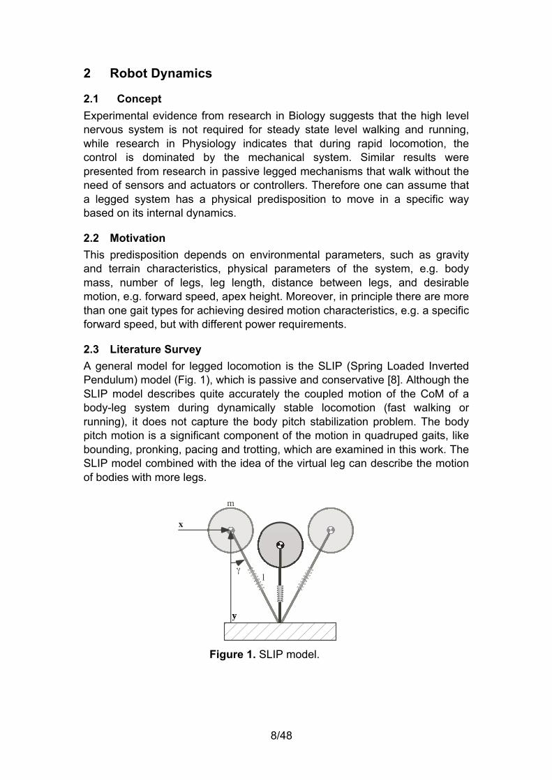
2.3 Literature Survey A general model for legged locomotion is the SLIP (Spring Loaded Inverted Pendulum) model (Fig. 1), which is passive and conservative [8]. Although the SLIP model describes quite accurately the coupled motion of the CoM of a body-leg system during dynamically stable locomotion (fast walking or running), it does not capture the body pitch stabilization problem. The body pitch motion is a significant component of the motion in quadruped gaits, like bounding, pronking, pacing and trotting, which are examined in this work. The SLIP model combined with the idea of the virtual leg can describe the motion of bodies with more legs.

Figure 1. SLIP model.

y

x

m

la

9/48

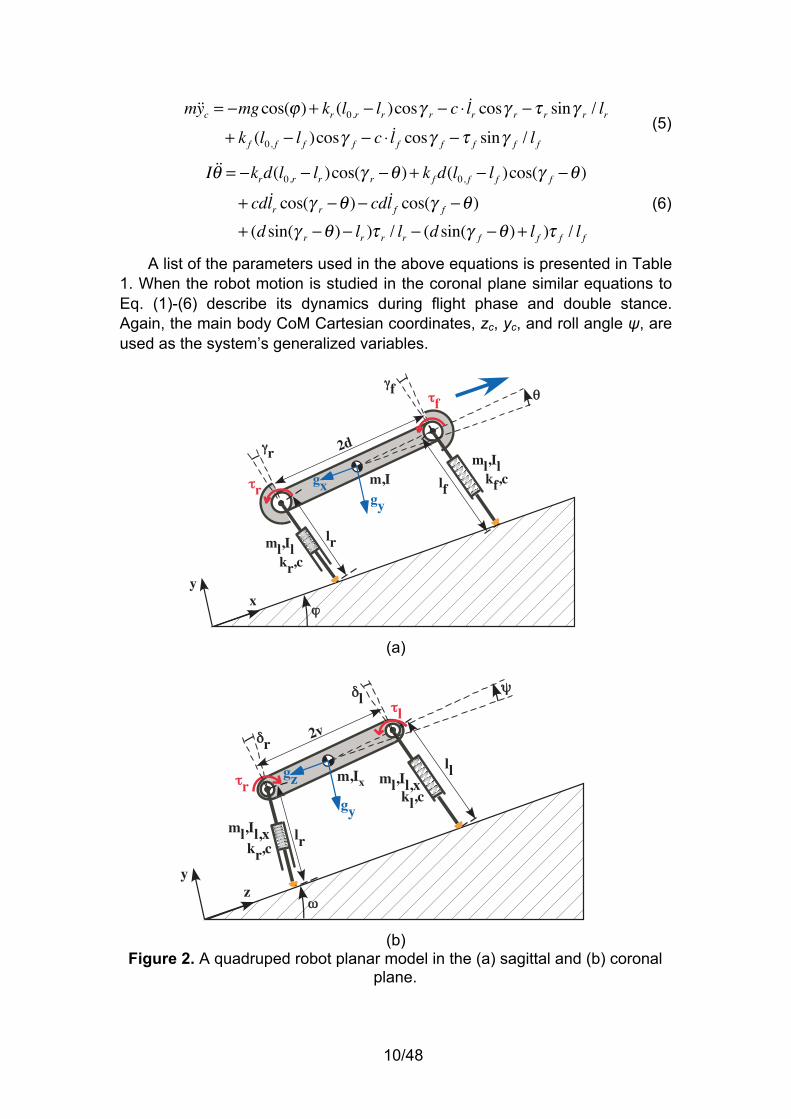
2.4 Contents of this work A lumped parameter model of a quadruped robot in the sagittal plane is shown in Fig. 2a and is used in the simulation set-up to deal with the body pitch stabilization problem. This model is consisted of two compliant virtual legs (VLegs) of mass ml and inertia Il and a body of m, I respectively. A VLeg, front or rear, models the two respective physical legs that operate in pairs when a gait is realized and has twice the mass, inertia, stiffness, and actuating requirement of each one of them [9]. Each VLeg is connected to the body with an actuated rotational joint at distance d from body’s CoM. The rotational hip joint allows positioning of VLegs at an angle γ in the plane of the forward motion. Also, each VLeg has a passive prismatic joint modelled as a linear compression spring of constant k and viscous damping coefficient c. The prismatic joint allows changes of the VLegs’ length l and energy accumulation during the robot’s motion. It should be noted here that front and rear VLegs are considered in general to have different uncompressed length l0 and compliance k.

A similar planar model can be considered in the coronal plane that holds the dynamics of the body rolling motion (Fig. 2b). The motion of the robot in this plane has a significant role in the overall stability of the motion because it is unlikely that in a highly unstructured terrain, like an asteroid surface, the left and right legs to be at the same level. Again, the model consists of two compliant virtual legs of mass ml and inertia Il,x around x-axis and a body of m, Ix respectively. In this model each VLeg, left or right, models the two respective physical legs of the same side and is connected to the body with an actuated rotational joint. The rotational hip joint allows positioning of VLegs at angle δ in the coronal plane (vertical to the plane of the forward motion). Also, each VLeg has a passive prismatic joint modelled as a linear compression spring of constant k and viscous damping coefficient c.

The robot motion was studied in the sagittal plane. During the flight phase (both VLegs do not touch the ground), the robot’s CoM performs a ballistic motion with constant system angular momentum H0 with respect to the CoM, and equations of motion given by,

xc = −gsin(ϕ ) (1)

yc = −gcos(ϕ ) (2)

H0 = (I + 2d2ml ) θ + (Ilm

2 + ll2mlm(m − 2ml ))( γ r − γ f ) /m

2 (3)

The robot dynamics for the double stance phase (both VLegs touch the ground) are derived using a Lagrangian approach. The main body CoM Cartesian coordinates, xc, yc, and pitch angle θ, are used as the system’s generalized variables. The double stance dynamics also yields the dynamics for the front and rear stance by removing terms that are not pertinent,

mxc = −mgsin(ϕ )− kr (l0,r − lr )sinγ r + c ⋅ lr sinγ r −τ r cosγ r / lr− k f (l0, f − l f )sinγ f + c ⋅ l f sinγ f −τ f cosγ f / l f

(4)

10/48

myc = −mgcos(ϕ )+ kr (l0,r − lr )cosγ r − c ⋅ lr cosγ r −τ r sinγ r / lr+ k f (l0, f − l f )cosγ f − c ⋅ l f cosγ f −τ f sinγ f / l f

(5)

I θ = −krd(l0,r − lr )cos(γ r −θ )+ k f d(l0, f − l f )cos(γ f −θ )

+ cdlr cos(γ r −θ )− cdl f cos(γ f −θ )+ (d sin(γ r −θ )− lr )τ r / lr − (d sin(γ f −θ )+ l f )τ f / l f

(6)

A list of the parameters used in the above equations is presented in Table 1. When the robot motion is studied in the coronal plane similar equations to Eq. (1)-(6) describe its dynamics during flight phase and double stance. Again, the main body CoM Cartesian coordinates, zc, yc, and roll angle ψ, are used as the system’s generalized variables.

(a)

(b)

Figure 2. A quadruped robot planar model in the (a) sagittal and (b) coronal plane.

af

yx

2d

lr

lf

ml,Il

ml,Il

of

kr,c

kf,c

gy

e

or

ar

gx m,I

bl

yz

2v

lr

ll

ml,Il,x

ml,Il,x

ol

kr,c

kl,c

t

gy

s

orgz m,Ix

br

11/48

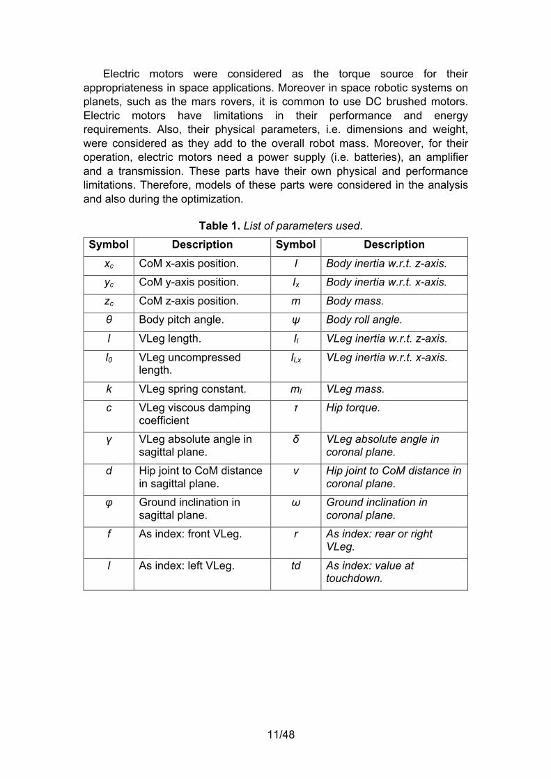
Electric motors were considered as the torque source for their appropriateness in space applications. Moreover in space robotic systems on planets, such as the mars rovers, it is common to use DC brushed motors. Electric motors have limitations in their performance and energy requirements. Also, their physical parameters, i.e. dimensions and weight, were considered as they add to the overall robot mass. Moreover, for their operation, electric motors need a power supply (i.e. batteries), an amplifier and a transmission. These parts have their own physical and performance limitations. Therefore, models of these parts were considered in the analysis and also during the optimization.

Table 1. List of parameters used.

Symbol Description Symbol Description xc CoM x-axis position. I Body inertia w.r.t. z-axis.

yc CoM y-axis position. Ix Body inertia w.r.t. x-axis.

zc CoM z-axis position. m Body mass.

θ Body pitch angle. ψ Body roll angle.

l VLeg length. Il VLeg inertia w.r.t. z-axis.

l0 VLeg uncompressed length.

Il,x VLeg inertia w.r.t. x-axis.

k VLeg spring constant. ml VLeg mass.

c VLeg viscous damping coefficient

τ Hip torque.

γ VLeg absolute angle in sagittal plane.

δ VLeg absolute angle in coronal plane.

d Hip joint to CoM distance in sagittal plane.

v Hip joint to CoM distance in coronal plane.

φ Ground inclination in sagittal plane.

ω Ground inclination in coronal plane.

f As index: front VLeg. r As index: rear or right VLeg.

l As index: left VLeg. td As index: value at touchdown.

12/48

3 Environmental Conditions

The environmental conditions affect the motion of a legged system, therefore it is necessary to develop mathematical models or concepts that shall quantify their relation with the emerging gaits. The environmental parameters that have direct effect on motion types are:

gravity, topographic features, surface characteristics and subsurface characteristics. Other parameters that have indirect effect but can be modelled sufficiently

by changing the characteristics of the body and legs are:

environmental radiation, temperature, pressure, corrosive environment, weather conditions of the celestial body. For example in the case of environmental radiation a larger mass would

correspond to the addition of a radiation protection system. On the other hand wind gusts can be modelled as external disturbances with which the controller must cope.

To this end, this analysis focuses on the first four parameters, which are the most crucial and cannot be modelled via an indirect way without loss of realism. In the coming sections, these four parameters are discussed in detail. Subsurface characteristics are a very intriguing issue on its own, and this particular matter is thoroughly developed. A model for simulating the leg-ground interaction is being proposed based on the literature on similar fields like terramechanics and impact mechanics, which is considered more appropriate for our purposes. Next, the algorithms used for simulation of the environment are presented.

3.1 Gravity This parameter plays a dominant role in the definition of the best strategy for gaits, as it was evident by the astronauts’ movements on the Moon. Gravity has direct implication on the motion of any multibody system, but even more on legged systems. At the limit of lack of gravity, no gait of any kind is possible. Additionally, gravity defines the apex height of the gait during dynamic motion. For example, a large stride may result in the landing of a robot far from the scientific point of interest. Table 2 displays the gravity for a number of celestial bodies.

Table 2 also includes the escape velocity. It is reasonable to assume that real danger exists mainly during motions on objects like asteroids, which have very small gravitational acceleration. This velocity actually represents an upper limit of rebound velocity after the impact with the ground of the legged robot. However and without loss of generality, this problem is considered less

13/48

severe for planets like Mars, therefore no particular limits are set in the simulations. However, the interested reader should have in mind this limit.

Table 2. Characteristics of some celestial bodies of interest [10].

Name Celestial Type g/gEarth Escape Velocity (km/s)

Weather Effects

Earth Planet 1.000 11.2 YES Moon Natural Satellite 0.163 2.4 NO Mars Planet 0.378 5.0 YES Jupiter* Planet 2.357 59.5 YES Titan Natural Satellite 0.138 2.6 YES Europa Natural Satellite 0.134 2.0 YES Itokawa Asteroid 0.00001 0.0002 NO Eros Asteroid 0.0006 0.0103 NO

*Jupiter is presented only as a reference, mainly for the gravitational parameter. Whilst gravity has a dominant role, the modelling of gravity is rather

simple. The dynamic model of the robot system explicitly includes the gravitational acceleration g . This is done by default during the formulation of the equations. Therefore in order to set the gravitational acceleration, the constant g is set prior to running the model according to the selection of the celestial body. For obvious reasons, there is no point in changing this constant while running a model.

3.2 Topographic Features The surface of celestial bodies is not flat and the slope on any area of interest is expected to be highly varied. Usually of great scientific importance are craters or similar features (e.g. mountain or volcanoes), and the inclination on these areas imposes various dangers for any robot (e.g. tipping over), especially when a dynamically stable gait is used, Fig. 3.

(a)

(b)

Figure 3. Topographic features of interest: (a) mountains and (b) craters.

To this end, it is necessary to model the inclinations so as to obtain

reliable results. More specifically, a general procedure has been developed both for 2D paths and 3D areas, Fig. 4. Each path is separated in small

14/48

segments with local inclinations (defined by the global inclination characteristics which can be variational or constant). The user defines only the dimensions of these segments, length for the 2D case, length and width for the 3D case. The dimensions are defined by the foot characteristics, which in this case the double of the diameter of the foot has been selected. In our case, a diameter of 20mm has been chosen, which leads to d = 2 ⋅20mm = 40mm length of segments. The same figures were selected for the width in the 3D case. Naturally this discretisation leads to a simplification when the foot lies on two consecutive segments at the same time, but without great loss of accuracy the simulation selects the most prominent of the two (the segment where the largest part of the foot lies). Of course by increasing or decreasing the dimension of the segment partitioning (for length or width), the user can configure the desired resolution. The properties of the terrain at xe,i or (xe,i , ze, j ) are defined by the properties of the segment they belong.

(a)

(b)

Figure 4. Discretisation in (a) 2D path and (b) 3D area.

3.3 Surface Characteristics The coverage of an area by rocks or soil, define the path profile of the robot. The rock dimensions are directly related to the gait that the robot should use to pass over without tipping. Moreover when touchdown occurs, it is highly possible some legs to be at a different level from the rest due to uneven terrain characteristics, such as different rock sizes. Various distribution models can be applied for this reason; for example for Mars, distribution model equations can be found in [11].

On the simulation side however, the existence of rocks can be modelled via changing locally and abruptly the local inclination. This can be easily done for example by adding an angle to the existing angle of a segment (due to local inclination), and then adding a negative angle of the same value on the next segment. However, it was considered that by using the proper controlled options, these abrupt alterations could be handled while the most significant problem is the main slope of the ground. For this reason, a user can add inclination spikes at the program (manually or automatically via the use of some random matrix), however in the rest of the analysis, this effect is not considered.

xi�1 xi xi+1xe,i

he,ihihi+1

d

�e,i

xi

xi+1xe,id

he,ij

ze, j z jz j+1

d

15/48

3.4 Subsurface Characteristics The terrain includes areas with regolith and bedrocks that can be comprised of materials with different properties [12]. Similar information can be obtained for other planets, satellites or asteroids. In addition, the compliance of the ground affects the motion and different contact models and/or parameters should be applied according to the nature of the terrain, e.g. granular soil could be implemented as a surface with large deformations, and a rocky surface as a fixed body with large stiffness. Stick, slip and sliding conditions should be taken into account, with surface friction playing dominant role for the proper characterization [13]. Since space agencies have shown in the past large interest in rover locomotion, various terramechanics models have been developed or exemplified for the case of planets, such as in [14]. Related work in the past took place for the case of legged locomotion with combined use of artificial intelligence schemes for real time estimation of soil parameters [15]. These works have as a common feature the use of equations that make use of the Bekker equations or similar. However, as [16] presents, this approach lags on the accurate representation of a dynamics interaction between soils and legs – and for this reason the authors introduce the term “terradynamics”. This approach is proved interesting for the locomotion of the robot types that the authors examine but does not include impact characteristics, which are prominent in our case. However the term terradynamics can be used here as well. Besides terradynamics, modelling of the interaction of legged robots with the ground during dynamic walking also includes impact mechanics.

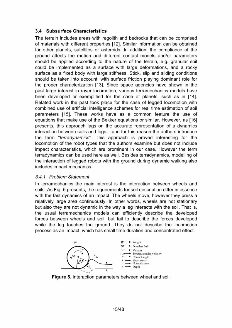
3.4.1 Problem Statement In terramechanics the main interest is the interaction between wheels and soils. As Fig. 5 presents, the requirements for soil description differ in essence with the fast dynamics of an impact. The wheels move, however they press a relatively large area continuously. In other words, wheels are not stationary but also they are not dynamic in the way a leg interacts with the soil. That is, the usual terramechanics models can efficiently describe the developed forces between wheels and soil, but fail to describe the forces developed while the leg touches the ground. They do not describe the locomotion process as an impact, which has small time duration and concentrated effect.

Figure 5. Interaction parameters between wheel and soil.

W

VDP

T ,�

��

x

�

W

VDP

T ,�

��

x

�

WeightDrawbar PullVelocityTorque, angular velocity

Normal stressShear stress

Depth

Contact angle

16/48

For example, the basic equations about relation of sinkage and pressure, which can be found in in literature, e.g. [14, 17] are based on Bekker or similar empirical equations in which the normal stress is given by:

σ x( ) = k1 + k2 ⋅b( ) ⋅ x b( )n (7)

where b is wheel width, k1,k2 constants depending on the material, x is sinkage and n the sinkage coefficient. On the other hand the equations concerning the shear stress, use the cohesion, c , and the friction angle φ which lead for example to the known equation which combines the above parameters and the maximum normal stress σ max with

τmax = c +σ max ⋅ tanφ (8)

However the focus of this study is dynamic walking, that is the legs nominally touch the ground for fractions of second. In contrast to static walking, the duration of time in which leg and soil interact is smaller. By this virtue, this interaction should be considered as an impact. Therefore, in order to efficiently analyze the interaction, impact mechanics procedures are necessary.

There are basically three approaches for analyzing such impacts. The first case employs the theory of rigid body impacts. The drawback in this case is that except for particular cases (e.g. solid terrain) this theory cannot produce reliable results. The second case employs compliant models. This case seems the most appropriate, as the different soil kinds can be simulated by lumped parameters (i.e. springs and dampers) with different linear or non-linear characteristics. Finally, one may employ the Finite Element Method (FEM); however this method requires a different procedure and large analytical representation of the soil elements per se, which would burden the simulation time and efficiency, add unnecessary complexity and of course would not allow the development of theoretical analysis that would be necessary to examine the problem. Furthermore, in the case a robotic controller is required to estimate the soil characteristics on the fly, FEM models are completely unacceptable. In other words a more appropriate method should be developed to overcome this problem, which is fast and reliable enough to be used during dynamic interaction of robots (or bodies in general) with a terrain (or a material in general). This approach must take into account the characteristics of the impact and the loss of energy. A novel method was proposed in [16]. This method is mainly applied to granular soils with particular characteristics. At its current form, it cannot simulate efficiently environments like wet terrain, whereas the concentrated force development of impact is not considered.

In this study, the compliant model for the normal direction of impact is prefered. The soil differences can be adopted easily by matching the stiffness and damping parameters to implicit characteristics of candidate soils. On the other hand the tangential force can be analyzed via a simpler rigid body model according to some basic assumptions, which are stated in the sequel.

17/48

Here, if a gait is not stable (i.e. due to soil characteristics the leg may slip), the simulation stops. Therefore the forces developed depend only on the geometry of the leg and the coefficient of friction µ . A more detailed model should take into account additional effects like tangential compliance, soil coherence and bulldozing.

The assumptions that apply in this research, considering the impact of legs on a ground are summarized:

i. The impact duration is very small and the impact forces very high. ii. Due to (i), the effects from external forces like gravity are

considered negligible. iii. The area of impact is localized, and thus small in comparison with

other dimensions. iv. Tangential effects are considered mainly due to friction and

geometrical characteristics of the leg under impact. Tangential compliance, coherence and bulldozing are not examined here.

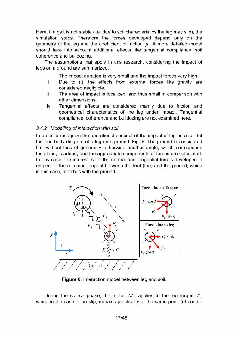
3.4.2 Modelling of interaction with soil In order to recognize the operational concept of the impact of leg on a soil let the free body diagram of a leg on a ground, Fig. 6. The ground is considered flat, without loss of generality, otherwise another angle, which corresponds the slope, is added, and the appropriate components of forces are calculated. In any case, the interest is for the normal and tangential forces developed in respect to the common tangent between the foot (toe) and the ground, which in this case, matches with the ground.

Figure 6. Interaction model between leg and soil.

During the stance phase, the motor M , applies to the leg torque T , which in the case of no slip, remains practically at the same point (of course

Ground

�

Kl

K C

Cl

l

T

y

+

x

FT

FT �cos�

FT �sin�

Fl �sin�

Fl �cos�Fl

M

m

Force due to leg

Force due to Torque

Fg

18/48

this is an assumption which is closer to the reality as the toe becomes smaller). Due to the falling motion, as the leg touches the ground, the main body continues its motion, which compresses the spring and the damper of the leg, Kl ,Cl respectively. Also the leg during touchdown has an initial angle θ in respect to the main body. The parameters K , C are the equivalent spring and damper parameters of the ground which represent its behaviour during impact (these values depend both on the ground and the material of the toe). The forces that act on the small mass which comes into contact with the ground are (the weight is omitted due to the impact):

- The force due to the torque:

FT = T l (9)

where l is the current length of the leg spring & damper - The force due to the spring and damper of the leg

Fl = Fl Kl ,Bl ,δ l,δ l

i⎛⎝

⎞⎠ (10)

where Fl is generally a non-linear equation depending on leg characteristics and the compression or restitution δ l and its speed, defined as

δ l = l0 − l (11)

with l0 the initial length of the leg. - The force due to the ground which is

Fg = Fg K ,B,δ y,δ y

i⎛⎝

⎞⎠ (12)

where Fg is generally a non-linear equation depending on the ground characteristics and the compression δ y and its velocity.

3.4.3 Impact dynamics between soil and leg The most intriguing part of simulating the interaction between the soil and a leg is the modelling of impact dynamics. The difficulties arise from the fact that to the best of the knowledge of the authors of this study, no unified approach towards the description of this kind of impact exists. On one hand, this is reasonable, as in general, different soil behave differently [18]. On the other hand some commonalities exist, which can be combined with well-established impact theory results, [19].

In fact, the problem is the dynamic nature of walking. The motion of the quadruped cannot be described via classic approaches of terramechanics. There is not a constant pressure from a tire, and the main driving force is the normal force of impact which in turn affects the tangential impact characteristics. On the other hand, static walking requires the stance phase duration to be several hundreds of milliseconds or even seconds, depending on the required forward velocity. Therefore this motion can be considered only partially as an impact. That is, dynamic walking requires a different approach which takes into account the fast dynamics of impact. As stated already at the

19/48

introduction of this chapter, the compliant model has been selected as a candidate for modelling the impacts.

First of all it is necessary to examine the existing models of this kind. Fortunately there are several ways to implement the viscoelastic impact. The two main models are the Kelvin-Voigt model, F = K ⋅ x + B ⋅ x (13) and the Hunt and Crossley model

F = K ⋅ xn + B ⋅ x ⋅ xn (14) where K ,B are the stiffness and damping coefficients of the ground, n a parameter which depends on the material and x the depth of penetration. It is known that the first model suffers from the fact that it starts and ends with discontinuity, and also that the force can take negative values, even if it is not a sticky or tensile terrain. Note that due to this modelling, the point where force crosses zero, has no physical meaning, and it is just a mathematical result. On the other hand, the Hunt and Crossley model, Fig.7, usually used with n = 3 2 to resemble a Hertzian contact, has been experimentally proven as a robust model for viscoelastic impacts, e.g. [20]. The area inside the curve represents the loss of energy during dissipation, and which is related with damping. In [18], the interested reader can find some more versions of non-linear models. It should be mentioned that the authors of [20] present an approach similar to the proposed solution, considering that the end of impact ends at a non-zero depth, still the implementation lacks in terms of generality: as their focus is in changing the damping parameters, the authors refer to some cases which cannot be efficiently modeled.

Figure 7. Impact curve using the Hunt- Crossley model.

Many researchers implement different approaches towards the more

accurate determination of the parameters of both models, and especially the non-linear Hunt and Crossley (HC) model. However, all approaches have some common characteristics.

! !"!!# !"!$ !"!$# !"!% !"!%#!

#!

$!!

$#!

!"#"$%&$'(#)*"+$,)-./

0#$"

%&1$

'(#

)2(

%1")

-3/)

0.+&1$)45'#6)74#$89%(55:";).(<":

&'()*+,'-+*./0+1+(+*23145+16'178998:.68'(

20/48

i. In general stiffness and damping can be non-linear functions. However as they describe the whole impact procedure, it is assumed that the impact starts and ends at x = 0 . That is the impact ends at the same position it begun.

ii. The case of a plastic deformation is not described. Theoretically this is correct from the point of view of strict viscoelastic description of the process. However, even in this case of plastic deformation, the behaviour of the material itself also has characteristics which can be modeled via lumped elements, without loss of generality.

iii. The case where the viscoelastic element has a delay in restitution (creepage) is not modelled via the non-linear model. In fact, that would not be a problem in very slow impacts, where the impacting solid almost «rests» on the material. That is the impact may end before the material reaches again x = 0 .

iv. It is known that terrains have specialized characteristics, which have to do with material properties, like behaviour under repetitive loading or compaction characteristics. For example consider the case of the wet soil at a beach. It is consistent with our understanding, that when we run on this soil, the surface sinks, and recovers for just a fraction, while we have to give more power to the legs to make the same motion, compared to the case where the surface were a solid material. This situation is not depicted in any non-linear model currently in use, and it is considered at the best case as an external disturbance.

Problems ii, iii and iv are examined in more detail, in the case of legged locomotion. As shown in Fig. 8, the spring element above the contacting mass m has an elongation according to the relative motion between m and the main body M . Using an HC model to examine the impact, it is reasonable to assume that the stance phase ends, when the surface of the material reaches again x = 0 . The spring then will have a particular elongation u1 , and of course, the analogous potential energy stored. However, the impact on a wet soil will end sooner than x = 0 , that is x > 0 (positive depth is considered towards the ground), and the elongation (and thus the potential energy stored) will be in general u2 ≠ u1 . This may introduce significant deviations from the first case, and must be taken into account in the controller, if possible not as a disturbance, but as part of the deterministic description of the controlled plant.

In order to fully understand the proposed model, it is imperative to examine again the impact phases, but under a different point of view. We start by examining the classical approach. Let us say we have a body M that hits the ground. At the moment of impact, the relative velocity between these is positive (towards the ground). As the body compresses the material the interaction force is increased, the depth is increased and the relative velocity is decreased. Note that in general, at non-linear viscoelastic models, the maximum force can be achieved before the end of the compression phase (see for example Fig. 6). When the relative velocity is zeroed, the maximum compression has been achieved. During restitution phase, the relative velocity

21/48

increases but in the opposite direction, the depth decreases, and the interaction force decreases. The most critical point here is how these two phases are separated – via the change of sign of the relative velocity. Note that the restitution ends when both x = 0 and interaction force is zeroed, but in fact this is due to the closed form of the impact models. What really matters is that the interaction force is zeroed or in other words, there is no contact between the impacting body and the terrain any more.

Now it is time to examine the proposed model, Fig. 8. As the body m comes into contact with the terrain, a fictional spring and damper that corresponds to the elastoplastic parameters of the contacting materials is compressed. As the compression proceeds, a part of the energy is stored to the spring, a part of the energy is dissipated through internal vibrations and other forms of energy loss and a part is dissipated because of the shape deformation. During compression this does not actually matter: the material that has been lost (e.g. via cratering around the impact point or compaction), “produced” their part of stiffness and damping and play no other role now.

As we reach the restitution phase, there is “less” material in the direction of motion, which might also become more stiff because of the compaction (or similar procedures). The spring now cannot be extended until the initial height (except it is a very sticky material), and also there is not so much elastic energy stored – the spring has been “broken”. The impact restitution phase will be “stiffer” and faster. In other words, we have a strong non-linearity in the fictional spring, which takes the form of a piecewise equation, between compression and restitution.

Figure 8. Different approaches of the usual viscoelastic models and the

proposed model.

Therefore, as the leg touches the ground, it feels the first fictional spring and damper. A classic HC model, until the point of maximum compression,

Impact Using Common Viscoelastic Models

Impact Using Proposed Model

Impact Compression Max. Compr. Restitution End of Impact

Impact Compression Max. Compr.Stiffness Change

Restitution End of Impact

22/48

can model this. At this point another stiffer spring should operate. The restitution phase begins. When the interaction force is zeroed, the impact has finished. Some notes are necessary:

I. Apparently a stiffer spring exerts a higher force for the same depth. An algebraic manipulation in order to have a smooth curve is required.

II. Theoretically there is the capability for the terrain, after the end of interaction, to have negative force. This negative force can be considered for example for grounds with creepage. Take for example an elastic terrain, which inherently delays its restitution. The end of the interaction with the impacted body does not coincide with the return of the terrain at its initial depth.

The final model has the following form for an impact instant “i”,

Fg =λc (i) ⋅K ⋅ xn + B ⋅ x ⋅ xn ,

λr (i) ⋅K ⋅ xn + B ⋅ x ⋅ xn + Fconst ,x ≥ 0x < 0

⎧⎨⎪

⎩⎪ (15)

where,

Fconst = K ⋅ xn ⋅ λc (i)− λr (i)[ ] (16)

and,

λr (i) ≥ λc (i) (17)

Eq. (17) is necessary for the model to have a physical meaning. Finally the interaction between m and the ground ends when no force exists anymore and at the same time this defines the final depth xe Fg = 0→ x = xe (18)

The above model has several advantages: I. The model can be used also with other models, like Kelvin-Voigt, or

models with non-linear dampers. It does not affect their performance, because it does not affect any of their properties. The use of the HC model is purely a choice of preference, because this model has been found to be very accurate on describing impact processes.

II. If the parameters in Eq. (17) are equal, then the model degenerates to a simple HC model. This means that the fictional spring of Fig. 8 retains its stiffness between compression and restitution.

III. After the impact at time “i” the soil has been compressed and its characteristics may change. For some materials, this can be characterized by:

λc (i) = λc (i +1) = λc (i + 2) = ...= 1λr (i) ≤ λr (i +1) ≤ λr (i + 2) ≤ ...

(19)

23/48

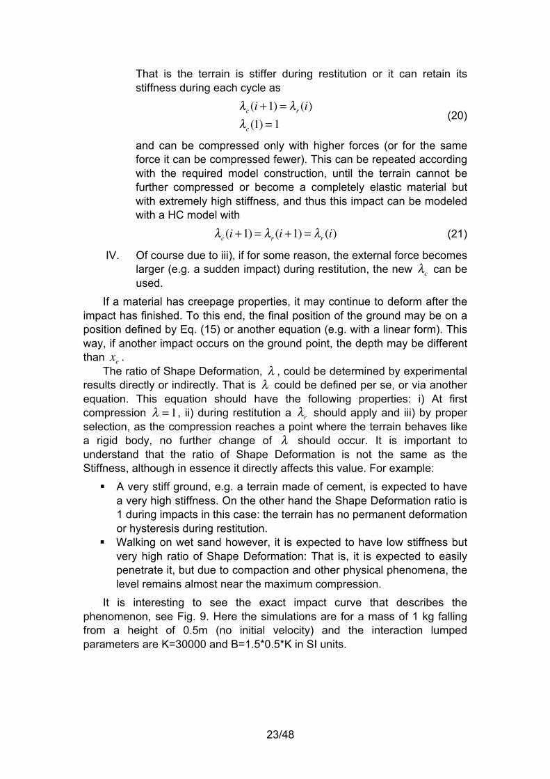
That is the terrain is stiffer during restitution or it can retain its stiffness during each cycle as

λc (i +1) = λr (i)λc (1) = 1

(20)

and can be compressed only with higher forces (or for the same force it can be compressed fewer). This can be repeated according with the required model construction, until the terrain cannot be further compressed or become a completely elastic material but with extremely high stiffness, and thus this impact can be modeled with a HC model with

λc (i +1) = λr (i +1) = λr (i) (21)

IV. Of course due to iii), if for some reason, the external force becomes larger (e.g. a sudden impact) during restitution, the new λc can be used.

If a material has creepage properties, it may continue to deform after the impact has finished. To this end, the final position of the ground may be on a position defined by Eq. (15) or another equation (e.g. with a linear form). This way, if another impact occurs on the ground point, the depth may be different than xe .

The ratio of Shape Deformation, λ , could be determined by experimental results directly or indirectly. That is λ could be defined per se, or via another equation. This equation should have the following properties: i) At first compression λ = 1, ii) during restitution a λr should apply and iii) by proper selection, as the compression reaches a point where the terrain behaves like a rigid body, no further change of λ should occur. It is important to understand that the ratio of Shape Deformation is not the same as the Stiffness, although in essence it directly affects this value. For example:

A very stiff ground, e.g. a terrain made of cement, is expected to have a very high stiffness. On the other hand the Shape Deformation ratio is 1 during impacts in this case: the terrain has no permanent deformation or hysteresis during restitution.

Walking on wet sand however, it is expected to have low stiffness but very high ratio of Shape Deformation: That is, it is expected to easily penetrate it, but due to compaction and other physical phenomena, the level remains almost near the maximum compression.

It is interesting to see the exact impact curve that describes the phenomenon, see Fig. 9. Here the simulations are for a mass of 1 kg falling from a height of 0.5m (no initial velocity) and the interaction lumped parameters are K=30000 and B=1.5*0.5*K in SI units.

24/48

Figure 9. Impact curve of the proposed model.

For λ = 1, the curve has the shape of the HC model. Increasing the Shape Deformation ratio, the exit point of the impact moves to the right.

Let now examine further the physical notion of the proposed impact model. To this end see Fig. 10. During compression (area “1”) the required energy includes the stored energy to the (in general) non-linear spring, the energy dissipated through waves or other sinks because of the (in general) non-linear damper and finally, the permanent deformation of the terrain at the particular point. If this deformation does not exists, then the restitution returns as in Fig.5. Similarly an area of dissipation due to various sinks but not permanent shape deformation near the impact point happens in area “2”. The model however takes into account the shape deformation near the impact point. The area numbered “3”, is the energy loss due to shape deformation, which cannot be restored.

Figure 10. Energy dissipation due to shape deformation and other means.

! !"!!# !"!$ !"!$# !"!% !"!%#!

#!

$!!

$#!

!"#"$%&$'(#)*"+$,)-./

0#$"

%&1$

'(#

)2(

%1")

-3/)

&$$"' ' $!

!%(+(4"5)0.+&1$)6(5"7)8(%)9&%'(:4) )

! !"!!# !"!$ !"!$# !"!% !"!%#!

#!

$!!

$#!

&'()*+,*-./0(12.3

41'*/+5*(36+.-+,2662)(12.3

!

"

#

$%&%'()'*+&,-%.'/,012

3&'%

()4'

*+&

,5+

(4%,

062,

7&)89:*:,+;,<&%(=9,-*::*.)'*+&

25/48

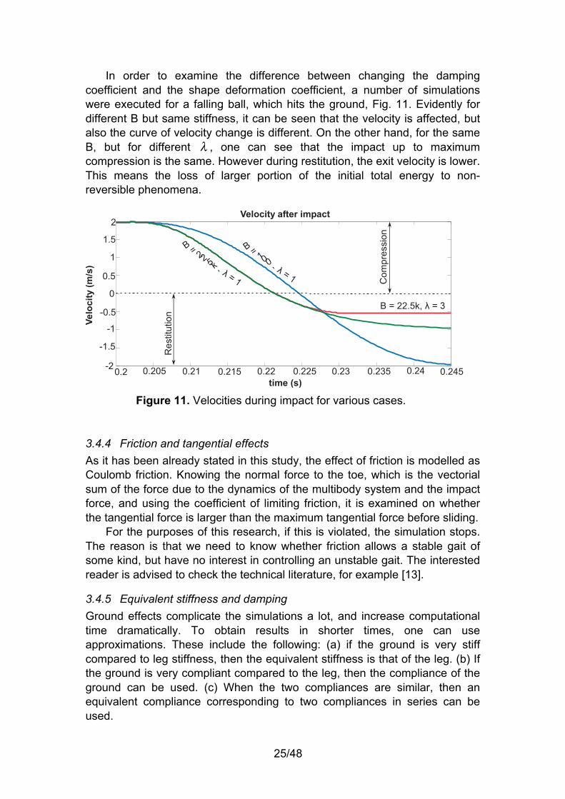
In order to examine the difference between changing the damping coefficient and the shape deformation coefficient, a number of simulations were executed for a falling ball, which hits the ground, Fig. 11. Evidently for different B but same stiffness, it can be seen that the velocity is affected, but also the curve of velocity change is different. On the other hand, for the same B, but for different λ , one can see that the impact up to maximum compression is the same. However during restitution, the exit velocity is lower. This means the loss of larger portion of the initial total energy to non-reversible phenomena.

Figure 11. Velocities during impact for various cases.

3.4.4 Friction and tangential effects As it has been already stated in this study, the effect of friction is modelled as Coulomb friction. Knowing the normal force to the toe, which is the vectorial sum of the force due to the dynamics of the multibody system and the impact force, and using the coefficient of limiting friction, it is examined on whether the tangential force is larger than the maximum tangential force before sliding.

For the purposes of this research, if this is violated, the simulation stops. The reason is that we need to know whether friction allows a stable gait of some kind, but have no interest in controlling an unstable gait. The interested reader is advised to check the technical literature, for example [13].

3.4.5 Equivalent stiffness and damping Ground effects complicate the simulations a lot, and increase computational time dramatically. To obtain results in shorter times, one can use approximations. These include the following: (a) if the ground is very stiff compared to leg stiffness, then the equivalent stiffness is that of the leg. (b) If the ground is very compliant compared to the leg, then the compliance of the ground can be used. (c) When the two compliances are similar, then an equivalent compliance corresponding to two compliances in series can be used.

!"#$%&'(!"# !"#!$ !"#% !"#%$ !"## !"##$ !"#& !"#&$ !"#' !"#'$

(#

(%"$

(%

(!"$

!

!"$

%

%"$

#

)*+

,-./

/0*1

2./

30343

0*1

5676%!!86

5676##"$986

5676##"$986

)$*

+,"

!-%&

#.'

(

)$*+,"!-%/0!$1%"#2/,!%

26/48

3.5 Computer Programs for Environmental Parameters

3.5.1 Ground Parameters In order to acquire robust conclusions about the effect of each environmental parameter to the gaits, two different approaches have been selected and therefore two different programs developed. In all cases one or more files can be produced with different

gravitational acceleration, slope, soil characteristics (equivalent stiffness, equivalent damping, coefficient

of friction). Note that all programs include extensive comments that make easy to the

user to understand their logic. Here for the sake of simplicity, only the main ideas are given. Additionally, if it is needed, the user can change the functions that create the values for each parameter, in order to increase randomness, etc.

3.5.2 Interactive Program The interactive program allows the user to define particular characteristics according to requirements, even the exact path. The user defines some basic characteristics and can select the kind of the terrain that is preferred.

More specifically, the program asks the user to define the kind of celestial body, the tolerance of the segments and the type of path or area (there is also the option to load a user-made path). The program processes the information and allocates characteristics to each segment. Then it plots the results and asks the user if it is needed to save the results for use on the multibody model.

File: mainenv.m

Functions: getcelest.m, pathdes.m, envselect2.m

3.5.3 Program for batch files creation The second program produces batches of files with various terrain characteristics. The user defines the minimum and maximum value for each parameter and the program covers all possible values according to some programming step (also user defined). For each combination of parameters a new file is being created.

This way it is more convenient to produce file batches in order to use them to create smooth mappings of the effect of each environmental parameter at the behavior of the quadruped, and makes easier for the researcher or the designer of such a robot, to find the operational point for each case of interest.

File: mainenvlight.m (for path), mainvenvlight3.m (for area) Functions: pathdeslight.m, envselectlight.m

27/48

3.5.4 Contact Interaction This is a function based on the proposed impact model, however by setting the Shape Deformation parameter equal to 1, a simple HC model is implemented. The algorithm examines if the impact started, if the maximum compression has been reached and whether the impact has finished or not. It has as inputs the position and velocity of each toe, and produces the impact force from the ground, which is the output back to the main multibody model of the legged robot.

This function is incorporated in the larger simulation of the legged robot and is being evoked every time the main program detects collision with ground. Note that this function is highly stiff mathematically; therefore for better results appropriate tolerances should be employed.

Function: Impact_Forces_Calculations_nim.m

28/48

4 Gait Classification

4.1 Concept Simulation-provided gaits were analysed with methods such the ones used in biological research. A classification was undertaken using the Hildebrand method.

4.2 Motivation The first level of classification using the gait diagram distinguishes gaits into symmetrical and asymmetrical. Symmetrical gaits have the footfalls of each pair of feet (front or rear) evenly spaced in time. Each foot of a pair contacts the ground for the same duration and usually fore contacts are the same as rear contacts. A gait diagram classifies the gaits according to two variables, one in each axis. The duration of the ground contact, or the duty factor, is expressed as a percentage of the cycle duration. For example, walking gaits in horses present a duty factor around value 60, which means that each foot in on the ground 60% of the cycle time and therefore, 40% of the cycle time off the ground. The second variable describes the phase difference between the rear and the front leg of the same side; again it is calculated as a percentage of the cycle time after which the front footfall follows the rear on the same side. Hildebrand plotted 1200 gaits for different animals in a single gait diagram and the result was a single irregular cloud proving that gaits are not discrete but they form a continuum.

4.3 Literature Survey Initial research on gait classification done by Muybridge lead to the support sequence [21], a sketch that indicates the sequence of combinations of supporting feet in each gait cycle. Although it is a simple and useful method, the support sequence does not show the relative durations of the various phases of the support that can differ in gaits with the same sequence. To deal with this shortcoming, Hildebrand introduced the gait diagram [22], which plots the support by each foot versus a time scale or a count of frames of the motion-capture video.

4.4 Contents of this work

4.4.1 Hildebrand Diagrams The simulation environment can provide the ordinate values of the CM of the robot, their respective time values and their respective phase indicator.

At first, we compute the time moment in which the evolution from the transient to the steady state occurs so as to be able to discriminate between these two phases of the robot locomotion. This is the time instance, for which, the pair of the local minimum value and the local maximum value of the robot CM ordinate coordinate, which appear first, after that, (i.e., the transitional time), contains exactly these two CM ordinate values, that differ from each one of the following local minimums and local maximums, respectively, less

29/48

than a user-defined tolerance. Here, we need to compute the vector that holds the indexes that correspond to both the local maximum and minimum values of the CM ordinate (versus time). We do this by detecting the monotonous (increasing or decreasing) sub-arrays that form the one-dimensional array of CM ordinate values, and then, we save the index of each ordinate value that is located between a couple of these sub-arrays. These sub-arrays are alternated sequentially, and that leads to an alternating finding of local maximums and minimums. We start by finding a maximum value, since the running process starts by dropping our robot from some height and with some initial horizontal velocity.

Secondly, we compute four vectors that hold the lift-off (lo) and touchdown (td) time instances of both the hind (back) and the fore (front) feet. In order to build these four vectors (”lo_hind” for the lo times of the hind feet, “td_fore” for the td times of the fore feet, and, similarly, “td_hind” and “lo_fore”), we check the succession of the phase indicators (integers in the range from one to four, 1 := double flight, 2 := back stance, 3 := double stance, 4 := fore stance) in a row-vector which is generated by the sets of differential equations, which are successively integrated in order to produce the simulated movement. According to the result of this check (different every time, in general) we update the appropriate time vector with the time value that corresponds to the last phase indicator which we inspected, before we detect a change in the values of the indicator vector, e.g., if at some part of this array the sequence of the indicators is […] 1 1 1 1 2 2 2 2 […], then we the update the td_hind vector with the time moment that is respective to the last “1” that appears.

To proceed, we calculate the three scalar quantities that form the gait diagrams. These quantities are the duty factors (DF’s) for both the hind and the fore feet and the phase relationship (PR) between the fore and hind ground contacts. For the computation of the DF’s (same procedure for both the hind and the fore feet), what we do is to compute every possible DF value that corresponds to one of the identified gait cycles of the robot motion, and then we consider their mean value as the final output value. We adopt this procedure because we want to calculate the most typical value of each DF.

The algorithm of computing one, of the many DF values, is fairly simple as it implements straight the definition schema [22]. For example, for the above-stated computation, we consider a pair of successive td time instances of a pair of feet and the unique lo event of the same pair of feet that is located between these two td events. In the end, we calculate the ratio of the time interval that separates the first (smaller of the two) td value from the lo value to the time interval between the two td values. We apply this for every pair of adjacent td incidents of the current pair of feet (hind or fore) and then we take their mean value as stated above.

Subsequently, we compute the value of the PR between the footfalls of the hind and fore feet. To do this, we implement two different methods.

The first is the classical method [22]. According to it, the value of the PR, of a gait, is equal to the ratio of the time interval between the td of the hind

30/48

feet and the td of the fore feet (where hind footfall precedes fore footfall, since the stride here is defined as the robot movement between two successive footfalls of the hind feet) to the time interval between the two successive landings of the hind feet.

The second is a variation of the classical method [23]. According to it, the PR value is equal to the ratio of the time interval between the td value of the fore feet and the td of the hind feet (here, the fore feet are used as reference in the definition of the gait cycle) to the time interval that separates the two consecutive touchdowns of the fore feet that are matched to the current gait.

To conclude, the PR computation is completed after we calculate every possible PR value, using both of the two pre-mentioned methods and after we consider as our final value the mean value of all realistic values that emerged.

Note that not all of the computed values are realistic. For example, if the fore feet hit the ground before the hind feet in the “beginning” of two successive gaits, and the “classic” computational method is employed, then a non-realistic value for the PR of the “first” gait is calculated. This is due to the fact that the touchdown incident of the fore feet of that gait is located very close to the second touchdown of the hind feet of the same gait, in proportion to its stride duration (the time interval between two successive footfalls of the hind feet). In other words, it is a percentage of 0% to 25%, which leads to a 75% to 100% value for the PR. For a similar reason, the value of the PR, computed using the alternate procedure, of the “first” gait of a couple of successive gaits where the hind feet touch the ground before the fore feet, in the beginning of that gait, is also non-realistic.

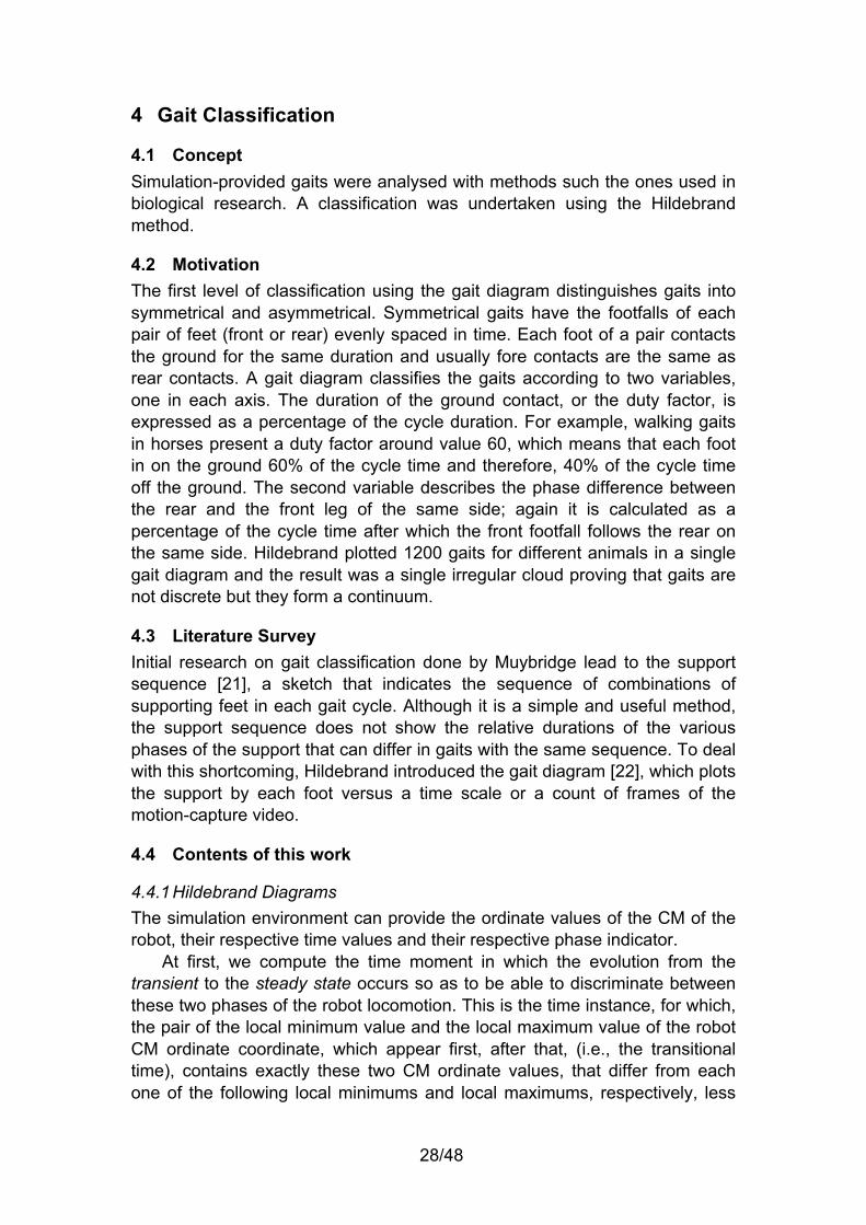
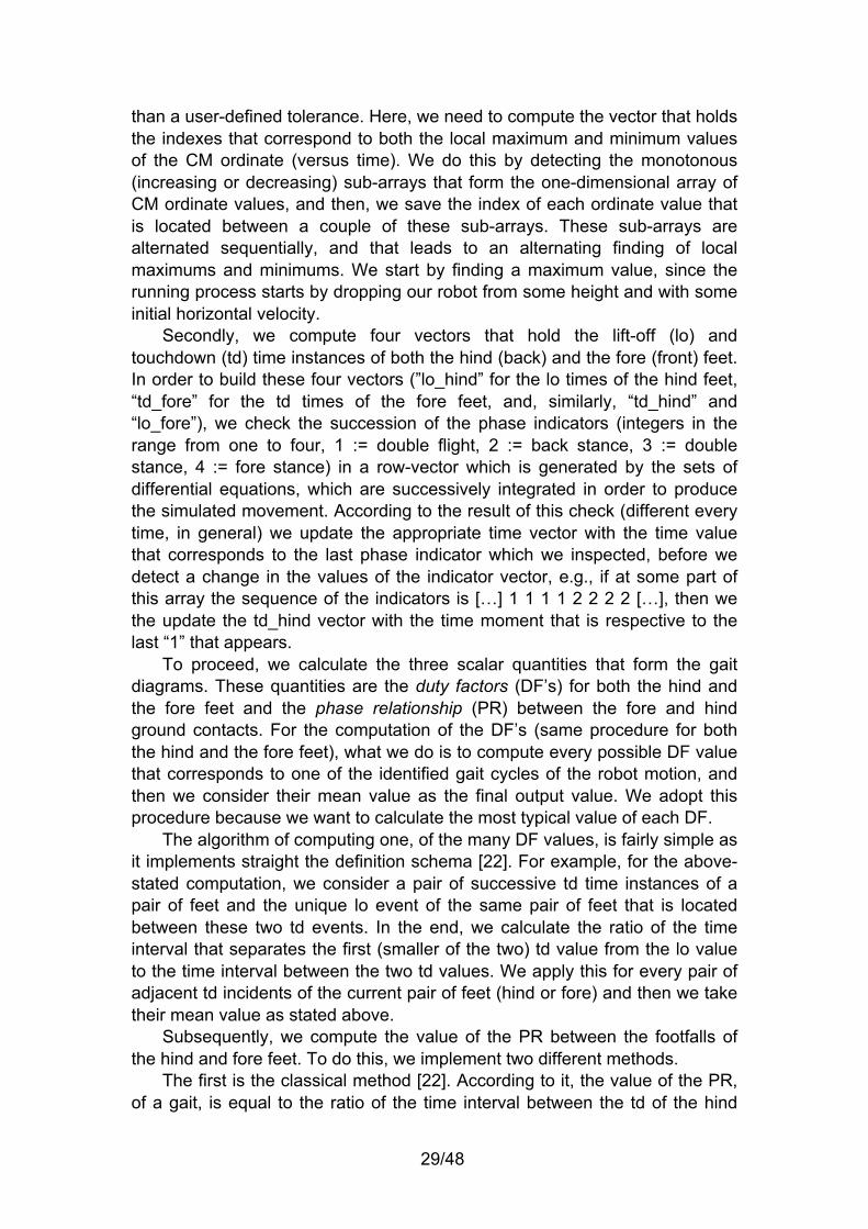
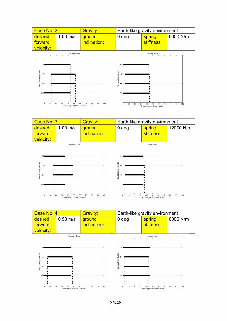
4.4.2 Results In this section, a number of characteristic Hildebrand Diagrams is presented for the Earth, Mars and the Moon, for the transient and the steady state states. Other variables that affect these include the desired forward velocity, the ground inclination and the leg spring stiffness. Case No: 1 Gravity: Earth-like gravity environment desired forward velocity:

1.00 m/s ground inclination:

0 deg spring stiffness

2200 N/m

0 10 20 30 40 50 60 70 80 90 100

RH

RF

LF

LH

Transient State

Percentage of Stride Duration

Feet

Loa

ding

Indi

cato

r

0 10 20 30 40 50 60 70 80 90 100

RH

RF

LF

LH

Steady State


Feet

Loa

ding

Indi

cato

r

31/48

Case No: 2 Gravity: Earth-like gravity environment desired forward velocity:



6000 N/m




12000 N/m




6000 N/m

0 10 20 30 40 50 60 70 80 90 100

RH

RF

LF

LH

Transient State


Feet

Loa

ding

Indi

cato

r

0 10 20 30 40 50 60 70 80 90 100

RH

RF

LF

LH

Steady State


Feet

Loa

ding

Indi

cato

r

0 10 20 30 40 50 60 70 80 90 100

RH

RF

LF

LH

Transient State


Feet

Loa

ding

Indi

cato

r

0 10 20 30 40 50 60 70 80 90 100

RH

RF

LF

LH

Steady State


Feet

Loa

ding

Indi

cato

r

0 10 20 30 40 50 60 70 80 90 100

RH

RF

LF

LH

Transient State


Feet

Loa

ding

Indi

cato

r

0 10 20 30 40 50 60 70 80 90 100

RH

RF

LF

LH

Steady State


Feet

Loa

ding

Indi

cato

r

32/48




9200 N/m




12000 N/m

Case No: 7 Gravity: Mars-like gravity environment desired forward velocity:



2800 N/m

0 10 20 30 40 50 60 70 80 90 100

RH

RF

LF

LH

Transient State


Feet

Loa

ding

Indi

cato

r

0 10 20 30 40 50 60 70 80 90 100

RH

RF

LF

LH

Steady State


Feet

Loa

ding

Indi

cato

r

0 10 20 30 40 50 60 70 80 90 100

RH

RF

LF

LH

Transient State


Feet

Loa

ding

Indi

cato

r

0 10 20 30 40 50 60 70 80 90 100

RH

RF

LF

LH

Steady State


Feet

Loa

ding

Indi

cato

r

0 10 20 30 40 50 60 70 80 90 100

RH

RF

LF

LH

Transient State


Feet

Loa

ding

Indi

cato

r

0 10 20 30 40 50 60 70 80 90 100

RH

RF

LF

LH

Steady State


Feet

Loa

ding

Indi

cato

r

33/48




3100 N/m




7400 N/m




1200 N/m

0 10 20 30 40 50 60 70 80 90 100

RH

RF

LF

LH

Transient State


Feet

Loa

ding

Indi

cato

r

0 10 20 30 40 50 60 70 80 90 100

RH

RF

LF

LH

Steady State


Feet

Loa

ding

Indi

cato

r

0 10 20 30 40 50 60 70 80 90 100

RH

RF

LF

LH

Transient State


Feet

Loa

ding

Indi

cato

r

0 10 20 30 40 50 60 70 80 90 100

RH

RF

LF

LH

Steady State


Feet

Loa

ding

Indi

cato

r

0 10 20 30 40 50 60 70 80 90 100

RH

RF

LF

LH

Transient State


Feet

Loa

ding

Indi

cato

r

0 10 20 30 40 50 60 70 80 90 100

RH

RF

LF

LH

Steady State


Feet

Loa

ding

Indi

cato

r

34/48




850 N/m




3900 N/m

Case No: 13 Gravity: Moon-like gravity environment desired forward velocity:



1780 N/m

0 10 20 30 40 50 60 70 80 90 100

RH

RF

LF

LH

Transient State


Feet

Loa

ding

Indi

cato

r

0 10 20 30 40 50 60 70 80 90 100

RH

RF

LF

LH

Steady State


Feet

Loa

ding

Indi

cato

r

0 10 20 30 40 50 60 70 80 90 100

RH

RF

LF

LH

Transient State


Feet

Loa

ding

Indi

cato

r

0 10 20 30 40 50 60 70 80 90 100

RH

RF

LF

LH

Steady State


Feet

Loa

ding

Indi

cato

r

0 10 20 30 40 50 60 70 80 90 100

RH

RF

LF

LH

Transient State


Feet

Loa

ding

Indi

cato

r

0 10 20 30 40 50 60 70 80 90 100

RH

RF

LF

LH

Steady State


Feet

Loa

ding

Indi

cato

r

35/48




1810 N/m




1810 N/m




2000 N/m

0 10 20 30 40 50 60 70 80 90 100

RH

RF

LF

LH

Transient State


Feet

Loa

ding

Indi

cato

r

0 10 20 30 40 50 60 70 80 90 100

RH

RF

LF

LH

Steady State


Feet

Loa

ding

Indi

cato

r

0 10 20 30 40 50 60 70 80 90 100

RH

RF

LF

LH

Transient State


Feet

Loa

ding

Indi

cato

r

0 10 20 30 40 50 60 70 80 90 100

RH

RF

LF

LH

Steady State


Feet

Loa

ding

Indi

cato

r

0 10 20 30 40 50 60 70 80 90 100

RH

RF

LF

LH

Transient State


Feet

Loa

ding

Indi

cato

r

0 10 20 30 40 50 60 70 80 90 100

RH

RF

LF

LH

Steady State


Feet

Loa

ding

Indi

cato

r

36/48




600 N/m




4000 N/m

0 10 20 30 40 50 60 70 80 90 100

RH

RF

LF

LH

Transient State


Feet

Loa

ding

Indi

cato

r

0 10 20 30 40 50 60 70 80 90 100

RH

RF

LF

LH

Steady State


Feet

Loa

ding

Indi

cato

r

0 10 20 30 40 50 60 70 80 90 100

RH

RF

LF

LH

Transient State


Feet

Loa

ding

Indi

cato

r

0 10 20 30 40 50 60 70 80 90 100

RH

RF

LF

LH

Steady State


Feet

Loa

ding

Indi

cato

r

37/48

5. Optimization

5.1 Concept In this part of the study, we analyse first quadruped robot gaits that result from an extensive search process. An optimization procedure using MathWorks fmincon is employed to determine the optimum motion initial conditions, quadruped model physical parameters and the desired motion parameters with respect to energy efficiency. Environmental conditions taken into consideration include gravity, topographic features, surface and subsurface characteristics. A point contact/ impact between foot and surface is assumed.

A number of figures are produced that depict the gait graphs resulting from simulations differing by a single significant parameter each time, e.g. leg stiffness. Resulting “multiple gait graphs” show that as gravity increases, the mean value of the Duty Factor also increases. Also, when ground inclination increases the Phase Relationship value increases, too. However, when leg stiffness increases the mean value of the Duty Factor decreases.

5.2 Motivation The extensive analysis using passive dynamic robot models and numerical return maps reveal fixed points, i.e. forward speed, apex height, pitch or roll rate, for different constant values of touchdown angles and for different gravity and soil properties. Using the same extensive analysis, the apex height and forward speed can have constant values according to mission requirements, while touchdown angles are the states of the searching procedure. This search answers the question, “which touchdown angles can achieve specific motion characteristics in different environments”. The methodology is employed and extended to different gravity environments (planets) to determine the conditions required to permit steady state cyclic motion.

5.3 Literature Survey Previous research showed that even simple passive planar models of a quadruped robot, like the one presented in Section 2.4 but without energy input (actuator torques) and losses, are able to capture a steady state behaviour without dependence on the details of the physical prototype [24], [25]. It was revealed, using numerical return map studies, that passive generation of a large variety of cyclic bounding motion is possible. Moreover, local stability analysis showed that the dynamics of the open loop passive system alone could confer stability of the motion.

5.4 Contents of this work

5.4.1 Extensive Search The extensive search scheme used in this work was set using the Matlab environment and has a two-layer structure. The inner layer involves the robot motion simulation. The equations of motion of each phase presented in Section 2.4 are solved using the ODE45 function. Which set of them is solved

38/48

each time is determined by the transition equations. The multipart controller function calculates during each flight phase the leg touchdown angles and actuator torques for the upcoming stance phase (rear, double or front). A simple PD-controller is used to position the legs to the calculated desired touchdown angles during the flight phase. The robot motion simulation was set to be terminated when the robot had completed 65 strides, i.e. complete cycles considered from a reference limb, e.g. rear left, flight phase till the next.

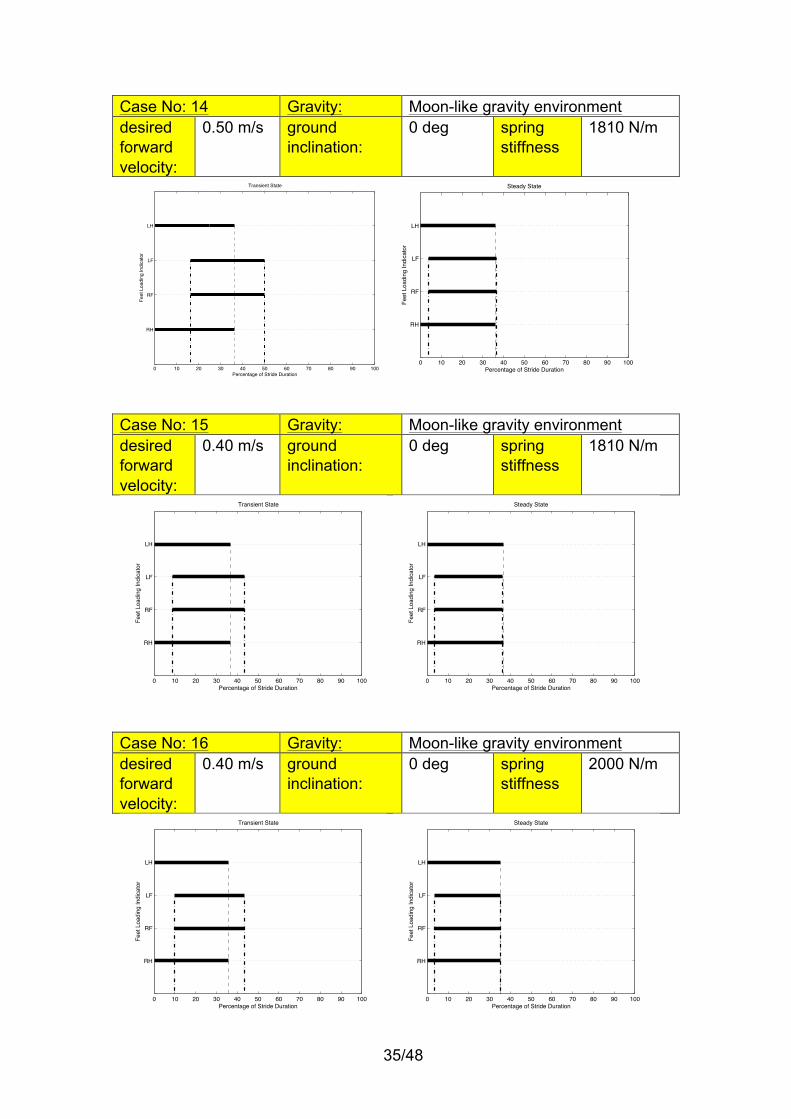
The outer layer involves definition of the initial conditions, the quadruped model physical parameters, the environment parameters and the desired motion parameters. This definition is programmed as a loop function to make the extensive search through a range of values of the parameters of interest feasible. In this work, parameters of interest include the uncompressed leg length and stiffness, gravity and ground inclination, quadruped forward velocity, while Table 3 displays the parameter values that were kept constant during the extensive search scheme.

Table 3. Constrained parameters during simulation.

Parameter Value Parameter Value Initial robot CM vertical position 0.35 m Body mass 9 kg

Initial body pitch 0 rad VLeg mass 0.62 kg

Initial body pitch rate 0.5 rad/s

Prismatic joint viscous friction

10 Ns/m

Initial vertical velocity 0 m/s Hip joint distance 0.50 m

Initial forward velocity 0.4 m/s Body inertia 0.56 kgm2

Desired robot CM apex height 0.32 m

5.4.2 MathWorks fmincon The initial conditions, the quadruped model physical parameters, the environment parameters and the desired motion parameters influence directly the robot motion and its characteristics. We seek to find their optimum values in order for the robot to traverse a specific distance while consuming the least amount of energy, which is directly associated to a measure of actuator torques. This corresponds to a constrained nonlinear multivariable problem, which can be solved using MathWorks fmincon and an appropriate problem formalization.

The optimization vector is chosen to be:

x = xcdes hdes x0 y0 θ0 k l0 d⎡

⎣⎤⎦ (22)

where xcdes and hdes are the desired robot forward velocity and apex height respectively, x0 , y0 and

θ0 are the initial forward velocity, vertical position and pitch rate respectively, while k , l0 and d are described in Table 1. The

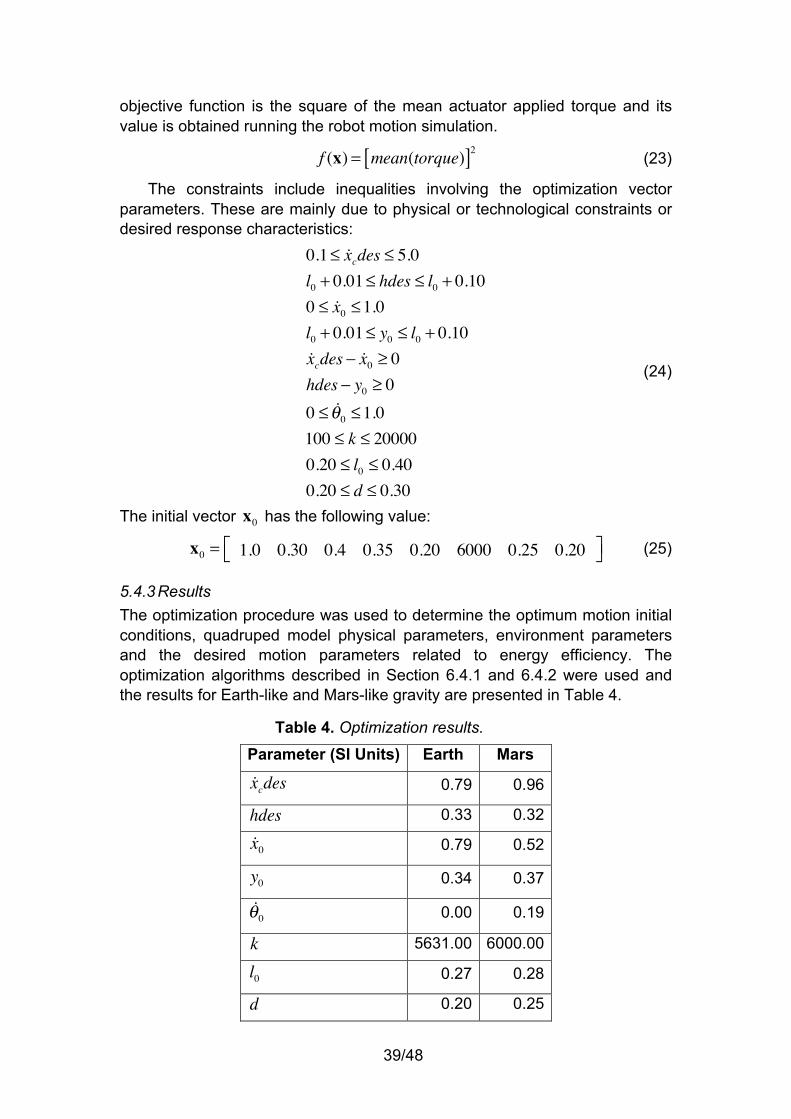
39/48

objective function is the square of the mean actuator applied torque and its value is obtained running the robot motion simulation.

f (x) = mean(torque)[ ]2 (23)

The constraints include inequalities involving the optimization vector parameters. These are mainly due to physical or technological constraints or desired response characteristics:

0.1≤ xcdes ≤ 5.0l0 + 0.01≤ hdes ≤ l0 + 0.100 ≤ x0 ≤1.0l0 + 0.01≤ y0 ≤ l0 + 0.10xcdes − x0 ≥ 0hdes − y0 ≥ 00 ≤ θ0 ≤1.0100 ≤ k ≤ 200000.20 ≤ l0 ≤ 0.400.20 ≤ d ≤ 0.30

(24)

The initial vector x0 has the following value:

x0 = 1.0 0.30 0.4 0.35 0.20 6000 0.25 0.20⎡⎣ ⎤⎦ (25)

5.4.3 Results The optimization procedure was used to determine the optimum motion initial conditions, quadruped model physical parameters, environment parameters and the desired motion parameters related to energy efficiency. The optimization algorithms described in Section 6.4.1 and 6.4.2 were used and the results for Earth-like and Mars-like gravity are presented in Table 4.

Table 4. Optimization results.

Parameter (SI Units) Earth Mars

xcdes 0.79 0.96

hdes 0.33 0.32

x0 0.79 0.52

y0 0.34 0.37

θ0 0.00 0.19

k 5631.00 6000.00

l0 0.27 0.28

d 0.20 0.25

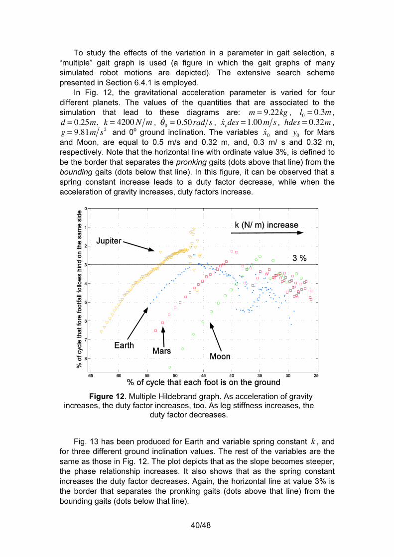
40/48

To study the effects of the variation in a parameter in gait selection, a “multiple” gait graph is used (a figure in which the gait graphs of many simulated robot motions are depicted). The extensive search scheme presented in Section 6.4.1 is employed.

In Fig. 12, the gravitational acceleration parameter is varied for four different planets. The values of the quantities that are associated to the simulation that lead to these diagrams are: m = 9.22kg , l0 = 0.3m , d = 0.25m, k = 4200N m ,

θ0 = 0.50 rad s , xcdes = 1.00m s , hdes = 0.32m , g = 9.81m s2 and 0o ground inclination. The variables x0 and y0 for Mars and Moon, are equal to 0.5 m/s and 0.32 m, and, 0.3 m/ s and 0.32 m, respectively. Note that the horizontal line with ordinate value 3%, is defined to be the border that separates the pronking gaits (dots above that line) from the bounding gaits (dots below that line). In this figure, it can be observed that a spring constant increase leads to a duty factor decrease, while when the acceleration of gravity increases, duty factors increase.

Figure 12. Multiple Hildebrand graph. As acceleration of gravity

increases, the duty factor increases, too. As leg stiffness increases, the duty factor decreases.

Fig. 13 has been produced for Earth and variable spring constant k , and for three different ground inclination values. The rest of the variables are the same as those in Fig. 12. The plot depicts that as the slope becomes steeper, the phase relationship increases. It also shows that as the spring constant increases the duty factor decreases. Again, the horizontal line at value 3% is the border that separates the pronking gaits (dots above that line) from the bounding gaits (dots below that line).

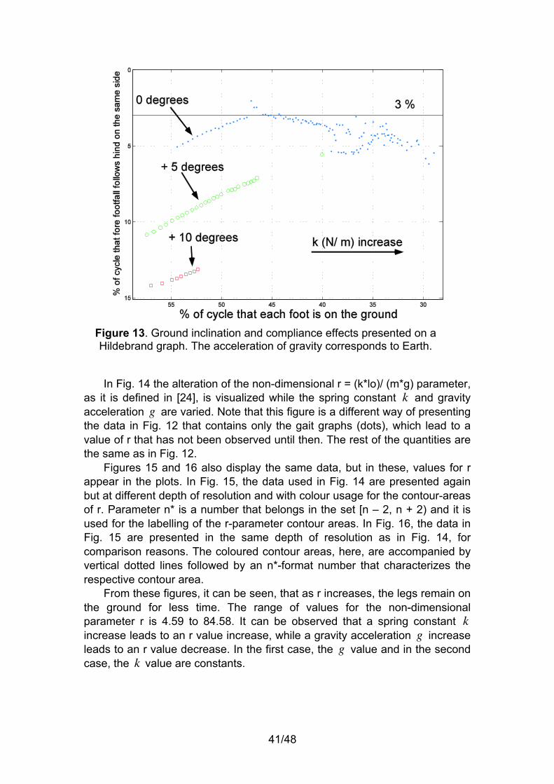
41/48

Figure 13. Ground inclination and compliance effects presented on a Hildebrand graph. The acceleration of gravity corresponds to Earth.

In Fig. 14 the alteration of the non-dimensional r = (k*lo)/ (m*g) parameter, as it is defined in [24], is visualized while the spring constant k and gravity acceleration g are varied. Note that this figure is a different way of presenting the data in Fig. 12 that contains only the gait graphs (dots), which lead to a value of r that has not been observed until then. The rest of the quantities are the same as in Fig. 12.

Figures 15 and 16 also display the same data, but in these, values for r appear in the plots. In Fig. 15, the data used in Fig. 14 are presented again but at different depth of resolution and with colour usage for the contour-areas of r. Parameter n* is a number that belongs in the set [n – 2, n + 2) and it is used for the labelling of the r-parameter contour areas. In Fig. 16, the data in Fig. 15 are presented in the same depth of resolution as in Fig. 14, for comparison reasons. The coloured contour areas, here, are accompanied by vertical dotted lines followed by an n*-format number that characterizes the respective contour area.

From these figures, it can be seen, that as r increases, the legs remain on the ground for less time. The range of values for the non-dimensional parameter r is 4.59 to 84.58. It can be observed that a spring constant k increase leads to an r value increase, while a gravity acceleration g increase leads to an r value decrease. In the first case, the g value and in the second case, the k value are constants.

42/48

Figure 14. Compliance - gravity effect on a Hildebrand graph as a

function of the dimensionless parameter r. The vertical lines correspond to fixed r values, indicated by the figure next to them.

Figure 15. Compliance – gravity (non-dimensional r) Hildebrand

graph. Coloured contour areas.

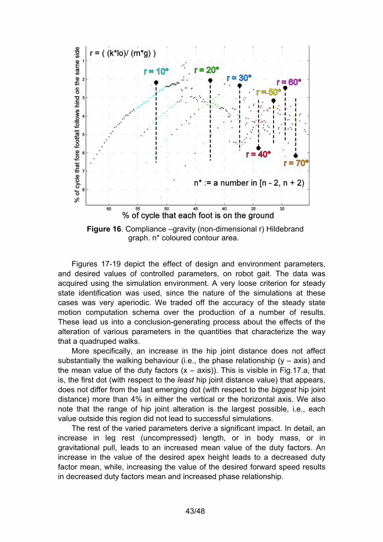
43/48

Figure 16. Compliance –gravity (non-dimensional r) Hildebrand

graph. n* coloured contour area.

Figures 17-19 depict the effect of design and environment parameters, and desired values of controlled parameters, on robot gait. The data was acquired using the simulation environment. A very loose criterion for steady state identification was used, since the nature of the simulations at these cases was very aperiodic. We traded off the accuracy of the steady state motion computation schema over the production of a number of results. These lead us into a conclusion-generating process about the effects of the alteration of various parameters in the quantities that characterize the way that a quadruped walks.

More specifically, an increase in the hip joint distance does not affect substantially the walking behaviour (i.e., the phase relationship (y – axis) and the mean value of the duty factors (x – axis)). This is visible in Fig.17.a, that is, the first dot (with respect to the least hip joint distance value) that appears, does not differ from the last emerging dot (with respect to the biggest hip joint distance) more than 4% in either the vertical or the horizontal axis. We also note that the range of hip joint alteration is the largest possible, i.e., each value outside this region did not lead to successful simulations.

The rest of the varied parameters derive a significant impact. In detail, an increase in leg rest (uncompressed) length, or in body mass, or in gravitational pull, leads to an increased mean value of the duty factors. An increase in the value of the desired apex height leads to a decreased duty factor mean, while, increasing the value of the desired forward speed results in decreased duty factors mean and increased phase relationship.

44/48

(a) (b)

Figure 17. (a) Hip joint distance and (b) leg uncompressed length effect Hildebrand graph.

(a) (b)

Figure 18. (a) Gravitational pull and (b) body mass effect Hildebrand graph.

(a) (b)

Figure 19. (a) Desired forward speed and (b) desired apex height effect Hildebrand graph.

45/48

5.5 Computer Programs for Gait Graphs and Optimization To produce the results in Chapters 4 and 5, a number of Matlab files were used. These include: • Extensive search:

quadruped_sim_1_5.m quadruped robot motion simulation quadruped_sim_5.m parameters of interest definition

• Optimization: quadruped_sim_1_5.m quadruped robot motion simulation quadruped_sim_2_5.m quadruped robot motion simulation with

objective function calculation func_1.m objective function calculation routine call opt_spacegaits.m starting point, constraints and environment

parameters definition.

46/48

6 Conclusions

Although research in legged robots over the last three decades led to several models, control algorithms and designs, a general systematic approach to the design and selection of appropriate gaits is lacking.

This work focused to the systematic use of Hildebrand gait diagrams in analysing gaits that are the result of an optimisation process according to criteria important for space missions, i.e. motion speed, energy efficiency, payload capability.

A lumped parameter model of a quadruped robot in the sagittal and the coronal plane, was obtained using the Lagrangian methodology, and used in a simulation set-up to tackle the body pitch/ roll stabilization problem. Appropriate models for the environment including gravity and soil properties were used. An optimization study based on an extensive analysis using numerical return maps and passive robot models used to determine the conditions required to permit steady state cyclic motion.

The results were evaluated using an appropriate objective function, an optimization algorithm and a complex robot model. The optimum gaits were classified using an automated scheme based on the Hildebrand diagrams.

A Hildebrand diagram computation procedure for legged robots has been developed. Combined with an extensive search scheme or an optimization procedure leads to optimum gait parameters and design guidelines.

The main results include the following:

As gravity increases the Mean Duty Factor increases. As ground inclination increases the Phase Relationship increases. As leg stiffness increases the Mean Duty Factor decreases.

Also, the range of the relative leg stiffness r value has been presented, under the variation of leg stiffness and gravity. The results show that:

As the spring constant k increases, the value of r increases. As gravity g increases the value of r decreases.

Overall, this study examined the effects of gravity, slopes, and stiffness to the gaits achieved by quadruped robots in dynamic walking and running. The study showed that it is possible to obtain stable gaits despite the varied conditions encountered in planetary exploration, and therefore, it indicates that legged robots can be used in such missions. It also presented important design guidelines that can be useful in designing robots able to complete their exploratory tasks successfully.

47/48

References [1] Heverly, M. and Matthews, J., “A Wheel-on-limb rover for lunar

operation,” i-SAIRAS 2008, Hollywood, USA, 2008. [2] Wheeler, D., Chávez-Clemente, D. and SunSpiral, V., “FootSpring:

A Compliance Model for the ATHLETE Family of Robots,” i-SAIRAS 2010, Sapporo, Japan, 2010.

[3] Görner, M., Chilian, A. and Hirschmüller, H., “Towards an Autonomous Walking Robot for Planetary Surfaces,” i-SAIRAS 2010, Sapporo, Japan, 2010.

[4] Younse, P., “Launchable and Retrievable Tetherbot Exploration System”, i-SAIRAS 2008, Hollywood, USA, 2008.

[5] Chacin, M. and Yoshida, K., “A Microgravity Emulation Testbed for Asteroid Exploration Robots,” i-SAIRAS 2008, Hollywood, USA, 2008.

[6] Bartsch, S., Birnschein, T., Cordes, F., Kühn, D., Kampmann, P., Hilljegerdes, J., Planthaber, S., Römmermann, M., and Kirchner, F., “SpaceClimber: Development of a Six-Legged Climbing Robot for Space Exploration,” ISR/ ROBOTIK 2010, Munich, Germany, 2010.

[7] Latta, M., Remy, C. D., Hutter, M., Höpflinger, M. and Siegwart, R., “Towards Walking on Mars,” Symposium of Advanced Space Technology in Robotics and Automation, ASTRA, Noordwijk, Netherlands, 2011.

[8] Full, R. J. and Koditschek, D., “Templates and Anchors: Neuromechanical Hypotheses of Legged Locomotion on Land,” Journal of Experimental Biology, 202, pp. 3325-3332, 1999.

[9] Raibert, M., Legged Robots That Balance. Cambridge, MA: MIT Press, 1986.

[10] http://nssdc.gsfc.nasa.gov/planetary/planetfact.html [11] ESA, MREP Mars Environmental Specification, SRE-

PAP/MREP/SFR-MES, Issue 1, Rev. 0, April 2010. [12] Golembek, M. P. et al, “The Martian Surface: Composition,

Mineralogy, and Physical Properties,” ed. J.F. Bell III. Cambridge University Press 2008.

[13] Stronge, W. J., “Impact Mechanics”, Cambridge University Press, 2000

[14] Iagnemma, K., Kang, S., Shibly, H. and Dubowsky, S., “Online Terrain Parameter Estimation for Wheeled Mobile Robots With Application to Planetary Rovers,” IEEE Transactions on Robotics, Vol. 20, No. 5, October 2004, pp. 921-927

[15] Caurin, G. and Tschichold-Gurman, N., “The development of a robot-terrain interaction system for walking machines,” IEEE ICRA 1994, vol. 2, 1994.

48/48

[16] Li, C, Zhang, T. and Goldman, D. I., “A Terradynamics of Legged Locomotion on Granular Media”, Science, 339, pp. 1408-1412, 2013

[17] Wong, J. Y., “Terramechanics and Off-Road Vehicle Engineering”, 2nd Edition, Elsevier, 2010.

[18] Gilardi, G. and Sharf I., “Literature Survey of Contact Dynamics Modelling”, Mechanism and Machine Theory 37, pp. 1213-1239, 2002

[19] Marhefka, D. and Orin, D., “A Compliant Contact Model with Nonlinear Damping for Simulation of Robotic Systems”, IEEE Transactions on Systems, Man and Cybernetics – Part A: Systems and Humans, 29(6), pp. 566-572, 1999.

[20] Azad, M. and Featherstone, R., “Modeling the Contact Between a Rolling Sphere and a Compliant Ground Plane,” ACRA 2010, Brisbane Australia, Dec 1-3, 2010.

[21] Muybridge, E., Animals in Motion. New York, NY: Dover, 1957. [22] Hildebrand, M., “The Quadrupedal Gaits of Vertebrates,”

BioScience, Vol. 39, No. 11, Animals in Motion, December 1989, pp. 766-775.

[23] Renous, S., Herbin, M. and Gasc J.-P., Contribution to the analysis of gaits: practical elements to complement the Hildebrand method, Comptes Rendus Biologies, vol. 327, 2004, pp. 99-103.

[24] Chatzakos, P. and Papadopoulos, E., “A Parametric Study on the Rolling Motion of Dynamically Running Quadrupeds,” IEEE MED 2009, Thessaloniki, Greece, 2009.

[25] Poulakakis, I., Papadopoulos, E. and Buehler M., “On the Stability of the Passive Dynamics of Quadrupedal Running with a Bounding Gait,” International Journal of Robotics Research, Vol. 25, Νο. 7, July 2006, pp. 669-688.

Ariadna Study: Space Gaits - esa.int Study Report/ACT-RPT-AI-ARI-12-52… · Ariadna Study: Space...

Documents

Transcript of Ariadna Study: Space Gaits - esa.int Study Report/ACT-RPT-AI-ARI-12-52… · Ariadna Study: Space...