fiILL C)PY UK-UNLIMITEDJ

ARETM(UHA)68512

Ln Octobaer 1988

L~~) COPY No. -

1-fPARISON OF INTEGRAL AND FINITE-DIFFERENCE METHODS

FOR PREDICTING THE TURBULENT BOUNDARY LAYER

ON AXISYMMETRICBODIES

O.J. ATKINS

This docum nt is the property of, 14r Majesty's Governmentand Crown copyright is reserved. R(-qlaests for permissson tod;sclost its contents outside offkiit Circles should, baddressed to the Issu;ng Authority

ADMIRALTY RESEARCH ESTABLISHMENTFE0718Procurement Executive, Ministry of. Defence

Queens Road. Teddington. Middlesex

1 ibY ~'\T:MET A UK-UNL IMI TED

ARE TM(1IHA)AH-,I.

COMPARISON OF INTEGRAL AND FTNITE-DIFFERENCE METHODSFOR PREDICTING THE TURBULENT BOUNDARY LAYER

ON AXISYMMETRIC BODIES

by

D J ATKINS

Predictions of the attached turbulent boundary layer onthree axisymmetric bodies were obtained usina integral andfinite-difference methods. The integral method was developed byMyring and the finite-difference method by Wang & Huang. Bothmethods take account of viscous-inviscid interaction effects andthe finite-difference method also takes account of the variationof static pressure across the boundary layer. Comparisons withexperimental data show both methods to be of similar accuracyover all but the last few per cent of the body length. However,the finite-difference method is marginally superior in thisregion and gives more detailed information, including theindividual velocity components and the Reynolds shear stress.

22 pages ARE (Teddin"ton)9 figures Queen's Road August 1988

Teddington Middx TWll OLN

CCopyright

Controller HMSO London1988

--p

CO0N TEN T S

1. Introduction

2. Theory

3. Comparison of theory with experiment

4. Conclusions and further research

Acc~rs1on For

'TIC' '7' &I

-3-

LIST OF SYMBOLS

C Skin-friction coefficient = (wall shear stress)/ApU e

H Shape factor = / iE

L Body length

RO Body radius at axial distance X from nose

R Radial distance from axis

UV Tangential and normal components of mean velocity

U'.V' Tangential and normal turbulent velocity fluctuations

Ue Velocity at edge of boundary layer

UINF Freestream velocity

UXUR Axial and radial components of mean velocity

X Axial distance from nose

Y Normal distance from body surface

XAngle of tangent to body surface with respect to axis

8 Boundary layer thicknessA|

8 Boundary layer displacement thickness

Displacement area = J (I-U/U e) (RO + Y cosm) dYM0 e

e Momentum area = f U/Ue(l-U/U ) (R0 + Y cos ) dY

J0 e e

, u I

I NTRODUCTION

Current ARE propulsor design methods for underwatervehicles require a knowledge of the boundary layer flow in theregion of the propulsor on the unpropelled vehicle. A typicalvehicle configuration often comprises a non-axisymmetric hullshape fitted with control fins, which results in a highly three-dimensional flow field with vortex shedding and high levels ofturbulence. Although such flow fields can be measured on scalemodels. the Reynolds numbers involved are usually considerablylower than the full-scale value, sometimes by a factor of 100.However, axisymmetric calculation methods can be used to givedesign information and estimate the boundary-layer Reynoldsnumber scaling effects.

An integral method for predicting' the tuirbulent boundarylayer on axisymmetric bodies, developed by Myring []], has beenin use at ARE for several years. The method was designedprimarily for predicting drag and has been shown to give goodresults for a wide variety of body shapes [2]. There is alsoreasonable aareement with experiment of the boundary-layerintegTral parameters and velocity profiles, which are required forpropulisor design purposes, on body shapes with small longitudinalcurvature and tail cone semi-aniles of less than about 201. Forbody shapes with fuller sterns, the agreement is less favourablewith the shape parameter in particular beina under-predicted atthe tail end of the body where the boundary layer may be close tosepa rat ion.

The present investigation aims to compare the Myring methodwith a more sophisticated finite-difference method developed byWang & Huang [3,4,51 and described in Section 2 below. Accuratemeasurements of the boundary-layer velocity components andReynolds stresses using hot-wire or laser-Doppler anemometry arenow available, and these are compared in Section 3 with pre-dictions using both integral and finite-difference methods forthree representative body shapes.

2. THIEORY

Roth the integral and the finite-difference method use thesame technique based on the displacement body concept, i.e. thestatic pressure or velocity at the edge of the boundary layer(required by the boundary-layer calculation) is the same as thesurface pressure or velocity in an inviscid flow over the bodysurface to which the displacement thickness has been added. Thismeans that the boundary-layer and potential-flow calculations canbe couipled together in an iterative cycle. The potential calcu-lation in both methods is based on the source panel method ofHess & Smith [61. The main difference between the two methods Isin the boundary-layer calculation. In the finite-differencemethod the momentum equation is solved directly, whereas in thejnt;egra] method it is formally integrated across the boundarylayer to give the momentum integral equation, which Is thensolved empirically.

-95

The Myring integral method proceeds as follows: the boundarylayer is calculated using an initial guess at the externalpressure distribution. The location of transition to turbulencemust be prescribed explicitly by the user. The potential flow isthen calculated over the "displacement surface" and the predictedpressure distribution is used as the input to the next boundary-layer calculation. The calculation is extended into the wake andsuitable end conditions are imposed. The profile drag isestimated from the momentum deficit in the far wake and theskin-friction dra* by integrating the local skin-frictioncoefficient over the body surface. An iterative scheme resultswhich stops when the iterated values of dracr have converged,usually after about six iterations. Profiles of the tangentialvelocity along a normal to the hull can be determined by assuminga power-law profile. The method has been adapted to include asimple actuator-disk representation of a lightly-loaded propeller[71.

The Wang & Huang method is based on the finite-differencesolution of the boundary-layer equations developed by Cebeci &Smith [8]. The location of transition can be prescribed orpredicted using a simple empirical method, and the effects of atripping device can be incorporated. A simple eddy-viscositymodel of turbulence is used, which is based on the traditionalmixing-length approach. The flow in the wake is calculated usinaan integral method proposed by Granville [9]. The displacementsurface is determined from the boundary-layer and wake calcu-lations, but in the body stern and near-wake regions a fifth-degree polynomial is used to connect the two displacementsurfaces. The iteration procedure starts with a potential flowcalculation over the body surface, and continues until themaximum change in the pressure coefficient on the displacementsurface is less than a specified tolerance, or the number ofiterations is exceeded. The results converge in an oscillatorymanner, and so the final pressure coefficient is usually taken tobe the average of the previous two values. The original versionof the method has been improved in two ways [5). Firstly, acorrection was made to the predicted velocity profiles to takeaccount of the variation of static pressure across the boundarylayer and to obtain the correct conditions at the freestreamboundary. Secondly, the turbulent mixing-length formulation wasmodified to include thick boundary-layer effects. Both modifi-cations are aimed at giving improved predictions in the propulsorregion at the stern of the body.

3. COMPARISON OF THEORY WITH EXPERIMENT

In this Section, brief details are given of boundary-layermeasurements on three axisymmetric bodies, and the measurementsare compared with integral and finite-difference method predic-tions. The body shapes are a prolate spheroid with conical tail,which was investigated by Patel et al (10), and two in-housebodies: a torpedo-shaped body with an inflected stern, known asthe propulsor research vehicle (PRV) E11] and a body with astreamline nose and tail cone with 15-degree semi-angle [121.Figure 1 shows the geometry and notation in the thick boundary

-6-

layer near the tail of a typical body, and the body shapeL;actually used are plotted as Figure 2.

The modified spheroid was investigated experimentally byPatel et al [10] in a low speed wind tunnel at Iowa Institute ofHydraulic Research. The tunnel speed was 40 ft/sec (12.2 m/s)

corresponding to a body-length Reynolds number of 1.26xl0 6 .Velocity and Reynolds stress measurements were conducted using ahot-wire anemometer, with the boundary-layer traverses beingnormal to the hull enabling direct comparison with boundary-layercalculation methods. In the present investigation, predictionsof the boundary-layer integral parameters and velocity profileswere obtained using both integral and finite-difference methods.Figures 3 and 4 show comparisons with theory of the measuredintegral parameters derived by integrating the velocity measure-ments across the boundary layer. Figure 9 shows comparisons ofthe tangential and normal velocity components as predicted by theintegral and finite-difference methods with hot-wire measure-ments. The integral method can only predict the tangentialcomponent. The finite-difference predictions here do not takeinto account the variation of static pressure across the boundarylayer. The integral method predictions agree well with themeasurements for X/L,0.93. At X/L=0.99, the finite-differencemethod is clearly superior to the integral method in predictingthe tangential velocity component. Figure 6 shows similarcomparisons with experiments of finite-difference predictions.both uncorrected and corrected to allow for static pressurevariation across the boundary layer. The improvement between theuncorrected and corrected profiles is only marginal for thetangential velocity component, but is more siqnificant for the

- normal velocity component, particularly near the edge of thea boundary layer. Figure 7 shows measurements and finite-differ-

ence predictions of the Reynolds shear stress. The agreement isgood up to X/L=0.90 but then falls off. This illustrates thedifficulty of using a simple eddy-viscosity model of turbulencein a thick axisymmetric boundary layer.

The propulsor research vehicle has a nose flat and bothprediction methods were modified slightly to account for this.Velocity measurements were carried out in the ARE 30-inch WaterTunnel at Teddington at a tunnel speed of 11 m/s corresponding to

a body length Reynolds number of 3x107 The body diameter was0.324m and the tunnel has a slotted wall working section 0.76m indiameter, so there may have been some small blockage effect.Boundary-layer velocity components were measured using a two-axislaser-Doppler system. Two traverses were undertaken, one movingin a horizontal direction, where the axial and radial componentswere measured, and the other in a vertical direction. where theaxial and circumferential components were measured. The tur-bulence levels were also estimated, but these were found to berelatively high because of the slotted wall.

The measurements of axial and radial velocity components arecompared with finite-difference predictions in Figure 8. Themeasured profiles are along radii and the predictions alongnormals to the hull. However examination of the predictionssuggest that the velocity profiles do not change significantly in

-7-

the distance spanned by the measured boundary layer and so nocorrection was applied. The finite-difference method is shown togive reasonable predictions of both the axial and radial velocitycomponents.

The body with the 15-decree tail cone was tested in the No 5Wind Tunnel at British Maritime Technology Ltd. at a body length

Reynolds number of 6.5xi06 . The main objective of the exper-iments was to study the wake of a body with fins, but somepreliminary measurements were carried out on the unappended body.The axial and radial velocity components were measured traversingthe boundary layer along a radius. The measurements were takenat one axial and seven radial locations and a complete circum-ferental traverse was obtained at 10 intervals. The purpose ofthis experiment was to ensure that any departures from axialsymmetry due to the effects of the supporting strut and wireswere minimal. Axial velocities were measured traversing in aradial direction. These are compared with finite-differencepredictions in Figure 9 and the agreement is generally favour-able.

4. CONCLUSIONS AND FURTHER RESEARCH

The Wang & Huang finite-difference and Myring integralmethods for predicting the turbulent boundary layer on axi-symmetric bodies have been evaluated against each other andcompared with experiment. The methods are found to be of similaraccuracy over all but the extreme tail end of a practical bodyshape. However the finite-difference method is marginallysuperior in this region because it takes some account of staticpressure across the boundary layer. The integral method can onlypredict the tangential velocity component, whereas the finite-difference method can predict the tangential and normal or axialand radial components and the Reynolds shear stress. However theintegral method is easier to use and produces much less outputthan the finite-difference method. The finite-difference methodis recommended for the majority of future computations, but somepreliminary calculations, for example, to investigate the effectof varying a parameter, are probably best performed using theintegral method.

There are several more sophisticated axisymmetric bodyprediction methods now available and a review of these hasrecently been carried out by Patel & Chen [13). For our currentbody shapes they appear to be only marginally more accurate thanthe finite-difference method but require significantly morecomputational effort. For practical vehicle configurationsincluding control fins and propulsor, a three-dimensionalReynolds-averaged Navier-Stokes calculation is necessary.Research into the relevant numerical methods is now in progressat ARE.

D J Atkins (SSO)

--8-

REFERENCES

1. MYRING, D.F. The profile drag of bodies of revolution insubsonic axisymmetric flow. Royal Aircraft Est TR72234(1973).

2. ATKINS, D.J. Assessment of a method for predicting the dragand boundary-layer development on a body of revolution atzero incidence. Admiralty Marine Technol Est AMTE(N)R78111(1979).

3. HUANG, T.T. et al. Propeller/stern/boundary-layer inter-action on axisymmetric bodies: theory and experiment.DTNSRDC Rep 76-0113 (1976).

4. WANG.H.T. & HUANG.T.T. User's manual for a FORTRAN IVcomputer program for calculating the potential flow/boundary-layer interaction on axisymmetric bodies.UDTNSRDC SPD-737-01 (1976).

5. HANG, H.T. & HUANG, T.T. Calculation of potential flow/boundary-layer interaction on axisymmetric bodies.Proc. ASME Symp. on Turbulent Boundary Layers. NiacgaraFalls. N. Y. (1979).

6. HESS, J.L. & SMITH. A.M.O. Calculation of potential flowabout arbitrary bodies. Progress in Aeronaut Sci, Voi 8,Pergamon Press (1966).

7. ATKINS, D.J. The effect of a propulsor on the hull boundarylayer of a body of revolution. Admiralty Marine Technol EstAMTE(N)TM79101 (1979).

8. CEBECI, T. & SMITH, A.M.O. Analysis of turbulent boundarylayers. Academic Press (1974).

9. GRANVILLE, P.S. The calculation of the viscous drag ofbodies of revolution. David Taylor Model Basin Rep 849(1953).

10. PATEL, V.C. et al. An experimental study of the thickturbulent boundary layer near the tail of a body ofrevolution. Iowa Inst of Hydraul Res Rep 142 (1973).

11. ARE Drawing no NI/1161.

12. ARE Drawings nos 0/2008/1-6 and Nl/1165.

13. PATE,. V.C. & CHEN, H.C. Flow over tail and in wake ofaxisymmetric bodies: review of the state of the art.J Ship Res 30(3)201-214 (1986).

Reports quoted are not necessarily available to members of thepublic or to commercial organisations.

-9-

I -J

ILI

IIz x

IDJ 0 <11 Z -A

>1 0 a

Ut 0

IA.

Ii 0

L LI00

-U 0II

I coTEi a'00

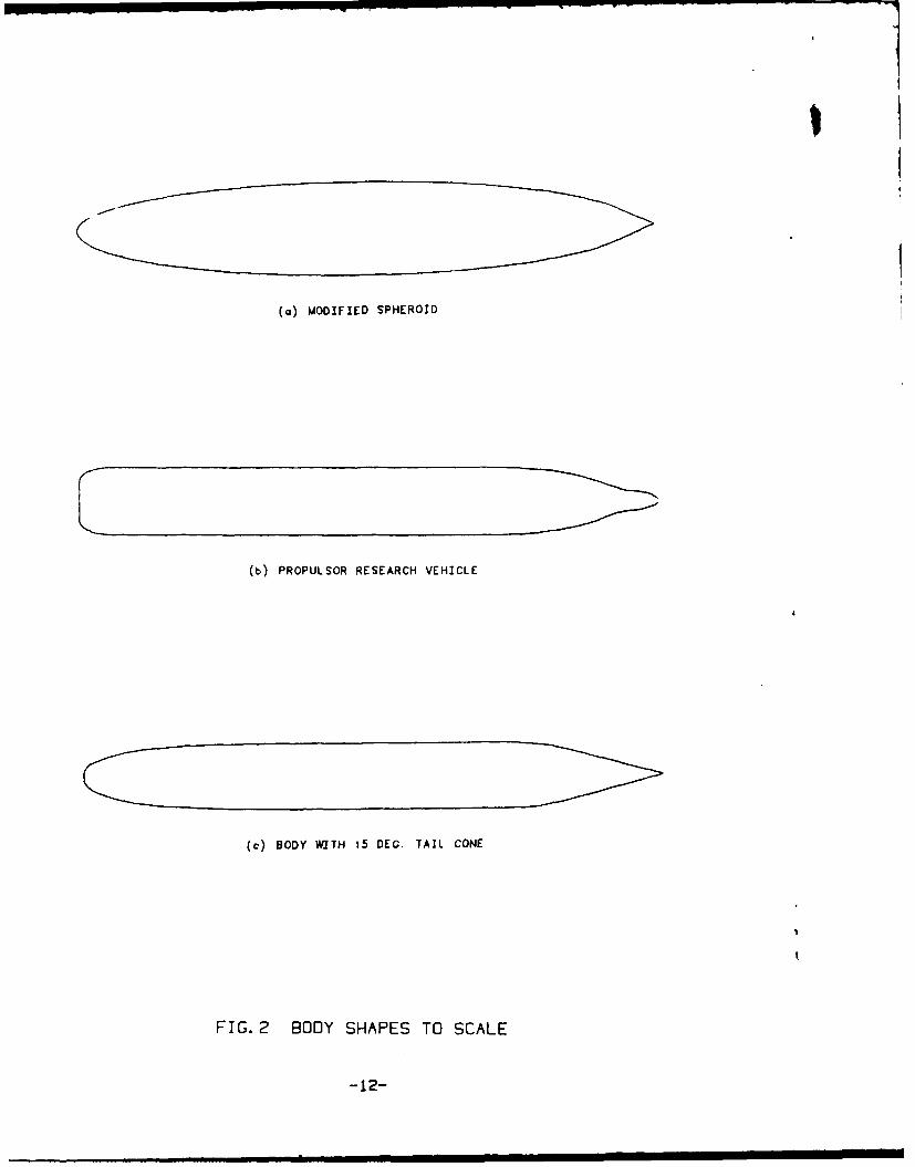
(a) MODIFIED SPHEROID

(b) PROPULSOR RESEARCH VEHICLE

()BODY WITH 15 DEC. TAIL CONE

FIG. 2 BODY SHAPES TO SCALE

-12-

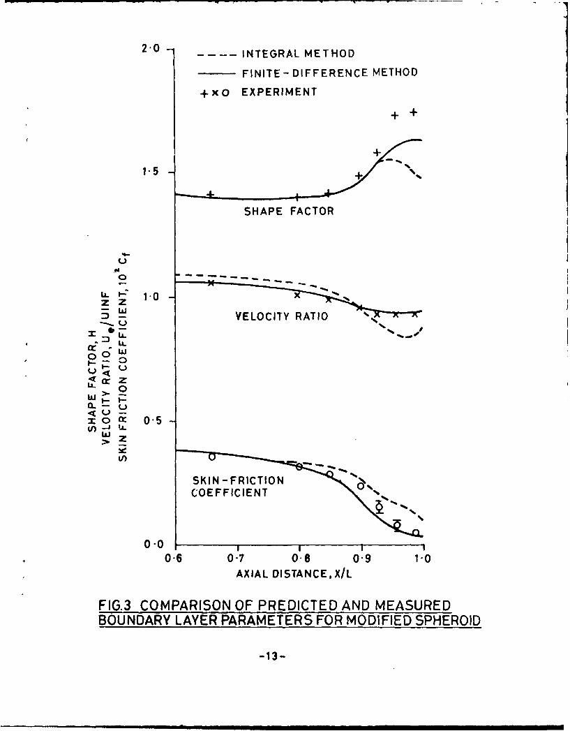
2-0 INTEGRAL METHOD

FINITE -DIFFERENCE METHOD

+xo EXPERIMENT

1.5

0

VELOCITY RATIO

~LL

a. t

U )-

06 07 06 95

FIG.3COMPAIN-FITO PRDITE ANMASRE

BOUNDARY LAYER PARAMETERS FOR MODIFIED SPHEROID

-13-

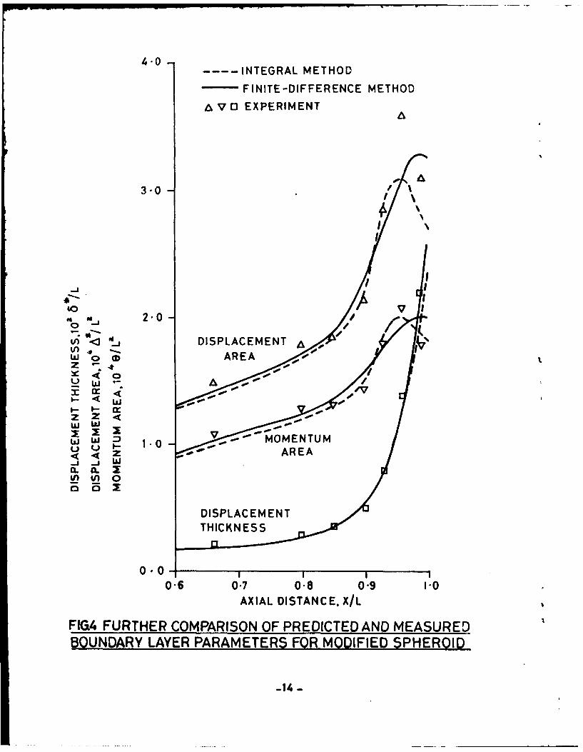
4.0---- INTEGRAL METHOD

- FINITE -DIFFERENCE METHOD

a VO1 EXPERIMENT

3-0

toI

Lfl ~ DISPLACEMENTA

I.- * .

zZw lop

w w D .o~ MOMENTUMU 1.0

DIAXIALMDITANE/

FlG4 FURTHER COMPARISON OF PREDICTED AND MEASUREDBOUNDARY LAYER PARAMETERS FOR MODIFIED SPHEROID

. INTEGRAL METHOD PREDICTIONS

FINITE-DIFFERENCE METHOD PREDICTIONS

x MEASUREMENTS (U/UINF)

+ MEASUREMENTS (V/UINF)

0.10 .X/L .0.85

+0.04 + x

+ xx 0.04* ~X+ X

X

* x0.04, 7 0.04

0.02 0.02

-80" 0.2 0.4 0.6 0.6 1.0 0.8%, 0.2 0.4 0.6 0.6 1.0

u/uXN. v/UYN u/iJzw. v/ulw

0.200- + / = 0.9 go 0.00 + = 0. 93

0.175 0.175" 40.150 " 0.150 "

0.125 + 0.12 +

,0.100- 0100

0.o7 + 0.075 ++

0.030- 0.050

0.025 0.025

.? 0080 0.2 0.4 0.6 0., 1.a 0 0 0.1 0 .4 0.4 ., 0., 1.0

u/u ,. v/uiw U/UNF, V/uIJW

0.30- X/L = 0.96 0.30 X/L = 0.99

0.25 0.25'

0.20- 0 .10- +++

O,.90" + 01 . 10- +,

4 +

/4 ~"/ o.@ *s

0.057 0.0: x /

08?o 0.1 0.4 0.$ 0.4, .0 0.2 0.4 0. 0.6 1.0

u/UJIw, v/ulf u/Uz. vluz

FIG.5 COMPARISON OF PREDICTED AND MEASURED TANGENTIAL

AND NORMAL VELOCITIES ON MODIFIED SPHEROID

-15-

SIICORRECTED FINITE-DIFFERENCE PREDICTIONS

UN-CORRECTED FINITE-DIFFERENCE PREDICTIONS

X MEASUREMENTS (U/UINF)

+ MEASUREMENTS (V/UNIF)

+ X/L = 0.80 0.1 X/L =0.85

+ Ic

0.04 + xx 0.0

xx0.04 x ~ 0.04

0.02 - 0.02

00. 0 .2 0.4 . 9, 1. 0 .. 0.2 0.4 0.0, 0.8 1.0

u/un,. V/UZNF tU/utr. V/uxw

0.200- = 0.90 0.20 = O. 93

o.17- /.,75 +

0.150 ". 150

0.1 I2 iI. 4125 + 0.125"

.0750 -.

075-0.1050- 0. O00-

0.05 ".002.5

08 0.2 0.4 0.0 o .0 0.2 0.4 0.4 0.3 1.0

u/ur. v/uNt u/u ,. v/uIN'

0.30- 1+ X/L 0. 96 0.20 / X/L = 0.99I /4./

/4.0.25 0.25

o. t - 4., +

/40.20- " 1/ 42 +

0. 10 0.10xIc +

_ x,

0.05 0.05 * I

0. 0.2 0.4 0., 0.8 1.0 0.80 0.2 0.4 0., 0.a 1.0

u/ua. v/urmr u/ui. v/uxw

FIG.6 COMPARISON OF FINITE-DIFFERENCE PREDICTIONS AND

MEASUREMENTS SHOWING EFFECT OF STATIC PRESSURE CORRECTION

(MODIFIED SPHEROID)

-16-

- FINITE-DIFFERENCE PREDICTIONS

M MEASUREMENTS

REYNOLDS SHEAR STRESS - UV'/WZNF*UINF)

0 X/L 0. 80 0.10 = 0.85

0.050.0"

0.06.- 0.04 A0.04- A

A

0 02 A 0.02

711h 0 0.023 0.050 0.075 0.100 0.125 0.150 0.175 0.200 80. 0.02 0.050 0.070 0.100 0.125 0,150 0.175 0.S00100 N REYNOLDS SHEAR STRESS 100 x REYNOLDS SHEAR STRESS

0.200 X/L = 0.90 o.oo0 X/L = 0. 93

0; 175 0.175

0.150 0.150

0.i15 0.115 A

N0.100- A . 0.100 A

AA

0.075- 0.070 A

0.050 A 0.050" 'A

.025 A a o0.025 A4AA

0?8o 0.010 0.000 0.075 0.100 0.125 0.150 0.175 0.200 0.025 0.050 0.075 0.100 0.120 0.150 0.170 0.200100 a REYNOLDS SHEAR STIRSS 100 V REYNOLDS SHEAR STRESS

0.,0 X/L 0.96 o.o X/L 0.99

0.25 0.25

0.20 0.20

TAA

A

0.015 A 0.10"

5: 8o 0. 02S'O *.SO'&. 07S 0. 100'0. 125'0. so'o, 173' 0. 200 S" 88O' 0. 025' 0. 030'0. 075'0. 100' 0. 125'0. 150O o. 17 O. 2o0000 0 REYNODS SHEAR STR.I0 100 v REYNOLDS SHEA PRESS

FIG. 7 COMPARISON OF PREDICTIONS AND MEASUREMENTS OF

REYNOLDS SHEAR STRESS ON MODIFIED SPHEROID

-17-

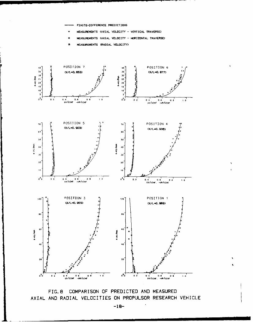
FINITE-DIFFERENCE PREDICTIONS

+ MEASUREMENTS (AXIAL VELOCITY - VERTICAL TRAVERSE)

* MEASUREMENTS (AXIAL VELOCITY - HORIZONTAL TRAVERSE)

* MEASUREMENTS (RADIAL VELOCITY)

40 POSITION 7 x e POSITION 6 + x

35 (X/L-O 853) 35 (X/L-O 877)3o-~~ JE30 .x

0 30- 4~*

+ 10£f 0 25 3 x.

0- + 20

00 0 0 2 . 4t 0 .1 0 8 1 0 0 0 " 0 .2 0 4 0 6 0 8 1 0

70" o-P S T O 4

15-5 " +

+x

+0 +

40 1* 0 +

0 + . + 4.

01 + * T - - -

00 02 04 0.6 0 8B 1 o00 0.2 0.4 0 6 0.6 10

UX/UINF. -UR/UINF UX/UINF, -UR/UINF

0 0 POSITION 6 + 00 POSITION 1

(X/LO. g5) (/L-O. g36,

60O 80"

6 0 x

~ x

:

~x

++ xx

60 60

so 50 +

40 40

300

+ x

++20 620

4WUI~. -,6 4rUXU~ . -O/UN

0I.8 OPAI.NO 0RDCE 4N.EAUE

TO + ++4

0 +

00 0 2 04 06 06 a a 00 0. 2 04 0. 6 0. a 4.0lUX/UINF. -UJ/Ulf4r UX/UINF, -Uft/UINF

AXIAL AND RADIAL VELOCITIES ON PROPULSOR RESEARCH VEHICLE

-18-

iiL095) +(/L099

Is soii i i••m / l •lH u

- FINITE-DIFFERENCE PREDICTIONS

-- ' MEASUREMENTS

140

120

100

II

40

2060

0.0 0.2 0.4 0.6 0.6 1.0UIC/uzN. -mJ/URN?

AXISYAETRIC BODY WITH 15 DEGREE TAIL CONE

FIG.9 COMPARISON OF PREDICTED AND MEASURED

AXIAL AND RADIAL. VELOCITIES

DISTRIBUTION

Copy No

D Sc (Sea)1

DD(U) ARE (Portland)2

DES Washington 3

CS (R) 2e Navy 4

ARE (Haslar) tJH 5

ARE (Haslar) UI-R 6

ARE (Haslar) UHU 7

ARE (Portland) UDU 8

ARE (Portland) UTW 9

DRIC 10-39

TEP ABC-17 40-45

RAE (Farnborouqh) Library 46

ARE (Haslar) Technical Information Centre 47-55

-21 -