ARE YOUR VARIABLE SPEED PUMPING APPLICATIONS

DELIVERING THE PREDICTED SAVINGS? IMPROVING CONTROL TO

MAXIMIZE RESULTS University of Dayton, Dayton, Ohio

Vijay Gopalakrishnan, Lead Engineer

Alexandra Brogan, Lead Engineer

Rohan Das, Research Assistant

Kelly Kissock, Ph.D., P.E., Director

Donald Chase, Ph.D., P.E., Chair

ABSTRACT

About one-fifth of all U.S. utilities incentivize variable frequency drives (VFDs) (NCSU

2014), and many of these drives control pumping systems. Field studies and research show that

few variable-flow systems are optimally controlled and the fraction of actual-to-ideal savings is

frequently as low as 40% (Kissock 2014a; Ma 2015; L. Song, Assistant Professor, Department of

Mechanical Engineering, University of Oklahoma, pers. comm., July, 2013.). Utility incentive

programs that rely on ideal energy saving calculations could overestimate savings by 30%

(Maxwell 2005).

Previous work has shown that excluding the effects of changing motor efficiency, VFD

efficiency, pump efficiency, and static head requirements results in overestimating savings

(Bernier and Bourret 1999; Maxwell 2005). This work considers the difference between actual

and ideal savings caused by bypass, position and setpoint of control sensors, and control

algorithms. This paper examines the influence of these factors on energy savings using

simulations, experimental data, and field measurements. In general, energy savings are increased

when bypass is minimized or eliminated, pressure sensors for control are located near the most

remote end use, and the pressure control setpoint is minimized.

INTRODUCTION

According to some estimates, pumps account for between 10% and 20% of world

electricity consumption (EERE 2001; Grundfos 2011). In industrial applications, pumps

frequently account for 25% of plant energy use (EERE 2001). Unfortunately, about two thirds of

all pumps use up to 60% too much energy (Grundfos 2011). A primary reason is that, although

pumps are designed for peak flow, most pumping systems seldom require peak flow and the

energy efficiency of flow control methods varies significantly. Before variable-frequency drives

(VFD), bypass and throttling were common, but inefficient, methods of varying flow to a

specific end use. Today, the most energy-efficient method of varying flow is by varying pump

speed with a VFD. Previous work has shown that excluding the effects of changing motor

efficiency, VFD efficiency, pump efficiency and static head requirements results in

overestimating savings (Bernier and Bourret 1999; Maxwell 2005).

The quantity of energy saved in variable-flow systems is highly dependent on other

factors in addition to motor, pump, and VFD efficiencies. Field studies and research show that

few variable-flow systems are optimally controlled and the fraction of actual-to-maximum

savings can be as low as 40% in poorly-controlled flow systems (Song 2013; Kissock 2014a; Ma

2015). In fact, it is not uncommon to find instances where VFDs actually increase energy use

when VFD efficiency losses are greater than pump power savings (Seryak, John. 2014. "Fan and

Pump System Low-Cost/No-Cost Energy Efficiency Opportunity Identification”. Triple Point

Energy Saving Seminar, Chillicothe, OH, April 10, 2014.).

This work considers the difference between actual and ideal savings caused by bypass,

position and setpoint of control sensors, and control algorithms. The paper begins by defining

“ideal” flow control as the most energy-efficient type of flow control, and compares pump power

from reducing flow by throttling to the ideal case. Since some minimum flow is required in most

pumping systems, the effect of bypass flow on pumping energy use is considered. The control

variable for most variable flow pumping systems is pressure; hence, the effect of the location and

setpoint value of pressure sensors on pump power is considered. Finally, a case study is

presented which demonstrates how pumping energy can be reduced through application of these

ideas.

IDEAL FLOW CONTROL

In order to consider the effect of bypass and control on pumping system energy use, it is

useful to define the maximum savings that can be expected from reducing flow. Figure 1 shows

two operating points of a pumping system. Point 1 represents the pump operating at full flow.

Point 2V is the operating point if pump speed is slowed by an optimally-controlled VFD. Point 2V

lies on a system curve in which dh (the pressure head) approaches zero as volume flow rate

approaches zero and pump head varies with the square of volume flow rate. This ideal case

represents the minimum pumping power that can be expected when flow is reduced from V̇1 to

V̇2. The reduction in pump power is also defined by the pump affinity law shown in Equation 1,

where W is fluid work and V̇ is volume flow rate at respective operating points.

𝑊2𝑉 = 𝑊1 × (�̇�2

�̇�1

)

3

1

Figure 1. The ideal system curve approaches zero head at zero flow.

Few actual pumping systems achieve the power reduction defined by the pump affinity

law because of throttling, minimum flow constraints, static head requirements due to changes in

elevation, velocity and pressure between the inlet and outlet of the piping system, and control

losses. In the following sections, these deviations from the ideal case are investigated.

THROTTLED FLOW CONTOL

One of the most common methods of varying flow is to throttle flow by partially closing

a valve in the piping system. In this section, we compare pump power from reducing flow by

throttling to reducing flow by slowing the pump with a VFD. The University of Dayton

Hydraulics Lab (UDHL) is equipped with two pumps, a VFD, a parallel piping network with

four branches, pressure sensors, and flow meters. In Figure 2, Point 1 is the operating point with

the pump at full flow. Point 2T is the operating point when flow was throttled to volume flow

rate, V̇2. Point 2V is the operating point when pump speed was slowed by a VFD to volume flow

rate, V̇2. Pump power is proportional to the product of head and flow, which is represented by the

rectangular area defined by each operating point. The data show that when flow was controlled

by throttling at Point 2T, the pump ran at 1,800 rpm and consumed 8.5 kW. When flow was

controlled by the VFD at Point 2V, the pump ran at 1,180 rpm and consumed 3.25 kW; pump

power decreased by 62%. Clearly, reducing flow with a VFD is more energy-efficient than

throttling flow.

Figure 2. Measured energy penalty due to throttled flow.

In pumping systems the power transmitted to the fluid, Wfluid, is given by Equation 2

where dh is the pressure head across the pump and V̇ is the volume flow rate.

𝑊𝑓𝑙𝑢𝑖𝑑[𝑘𝑊] =𝑑ℎ[𝑓𝑡 𝐻2𝑂 ] × 𝑉[𝑔𝑝𝑚]

3,960 [𝑔𝑝𝑚 ∙ 𝑓𝑡 ∙ 𝐻2𝑂/ℎ𝑝]× 0.746 [

𝑘𝑊

ℎ𝑝] 2

At Point 2V, the fluid work was:

𝑊𝑓𝑙𝑢𝑖𝑑[𝑘𝑊] =71.6 𝑓𝑡 𝐻2𝑂 × 81 𝑔𝑝𝑚

3,960 𝑔𝑝𝑚 ∙ 𝑓𝑡 ∙ 𝐻2𝑂/ℎ𝑝×

0.746 𝑘𝑊

ℎ𝑝= 1.09 𝑘𝑊

However, the electrical power to the pump motor is always greater than fluid work because of

efficiency losses in motor, pump, and VFD. Using the measured power draw and calculated fluid

work, the combined efficiency, ηcombined, is given by Equation 3.

𝜂𝑐𝑜𝑚𝑏𝑖𝑛𝑒𝑑 =𝑊𝑓𝑙𝑢𝑖𝑑[𝑘𝑊]

𝑃[𝑘𝑊] 3

At Point 2V, the combined efficiency was:

𝜂𝑐𝑜𝑚𝑏𝑖𝑛𝑒𝑑 =1.09 𝑘𝑊

3.25 𝑘𝑊× 100% = 34%

The combined efficiencies at Points 2T and 2V were 32% and 34%, respectively. These results

indicate that about 70% of pump power was lost due to inefficiencies in the motor, pump, and

VFD.

MINIMUM FLOW CONSTRAINTS

Most pumping systems require some minimum flow due to constraints such as minimum

VFD speed, minimum flow through the pump, or minimum flow through equipment such as a

chiller evaporator. Hence, a bypass is needed to provide a path for minimum flow when end uses

reduce flow below this minimum. In the ideal case, no bypass flow is permitted when the end

uses require more than minimum flow. Flow in excess of the minimum required flow increases

pumping power and wastes energy.

Ideal Bypass Flow Control

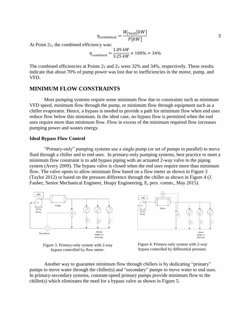
“Primary-only” pumping systems use a single pump (or set of pumps in parallel) to move

fluid through a chiller and to end uses. In primary-only pumping systems, best practice to meet a

minimum flow constraint is to add bypass piping with an actuated 2-way valve to the piping

system (Avery 2009). The bypass valve is closed when the end uses require more than minimum

flow. The valve opens to allow minimum flow based on a flow meter as shown in Figure 3

(Taylor 2012) or based on the pressure difference through the chiller as shown in Figure 4 (J.

Fauber, Senior Mechanical Engineer, Heapy Engineering, E, pers. comm., May 2015).

Another way to guarantee minimum flow through chillers is by dedicating “primary”

pumps to move water through the chiller(s) and “secondary” pumps to move water to end uses.

In primary-secondary systems, constant-speed primary pumps provide minimum flow to the

chiller(s) which eliminates the need for a bypass valve as shown in Figure 5.

Figure 3. Primary-only system with 2-way

bypass controlled by flow meter.

Figure 4. Primary-only system with 2-way

bypass controlled by differential pressure.

Chilled Water to End Uses

Secondary Pump

Constant Speed Primary Pump

VFD

dP

Chiller

Figure 5. Primary-secondary system eliminates the need for a bypass valve

Excess Bypass Flow

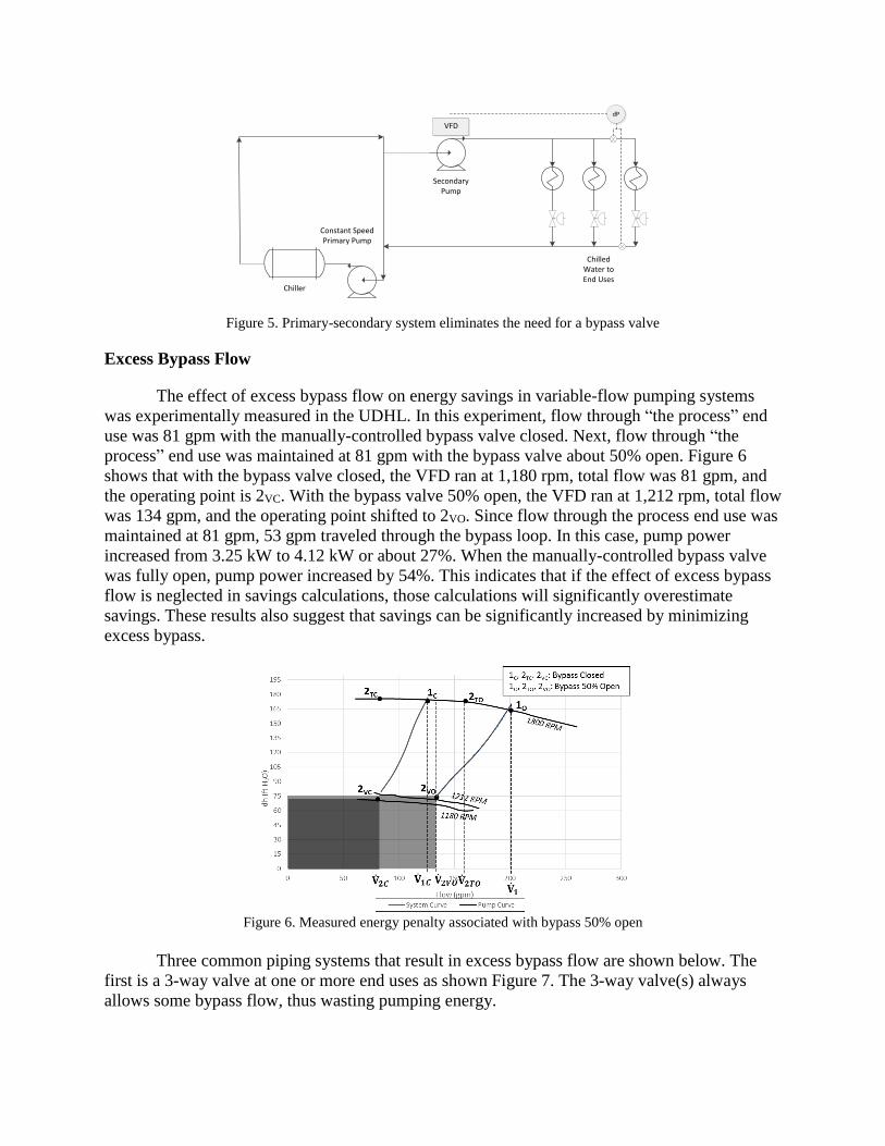
The effect of excess bypass flow on energy savings in variable-flow pumping systems

was experimentally measured in the UDHL. In this experiment, flow through “the process” end

use was 81 gpm with the manually-controlled bypass valve closed. Next, flow through “the

process” end use was maintained at 81 gpm with the bypass valve about 50% open. Figure 6

shows that with the bypass valve closed, the VFD ran at 1,180 rpm, total flow was 81 gpm, and

the operating point is 2VC. With the bypass valve 50% open, the VFD ran at 1,212 rpm, total flow

was 134 gpm, and the operating point shifted to 2VO. Since flow through the process end use was

maintained at 81 gpm, 53 gpm traveled through the bypass loop. In this case, pump power

increased from 3.25 kW to 4.12 kW or about 27%. When the manually-controlled bypass valve

was fully open, pump power increased by 54%. This indicates that if the effect of excess bypass

flow is neglected in savings calculations, those calculations will significantly overestimate

savings. These results also suggest that savings can be significantly increased by minimizing

excess bypass.

Figure 6. Measured energy penalty associated with bypass 50% open

Three common piping systems that result in excess bypass flow are shown below. The

first is a 3-way valve at one or more end uses as shown Figure 7. The 3-way valve(s) always

allows some bypass flow, thus wasting pumping energy.

Figure 7. 3-way bypass valve at one end use.

Another piping system that allows excess bypass flow uses a manually-controlled bypass

valve as shown in Figure 8. Manually-controlled valves are always at least partially open and

hence allow bypass flow even when no bypass is required. The recommended commissioning

practice in a system with a manually-controlled bypass valve is to close all end use loads and

throttle to allow minimum required flow (J. Kelley, Energy Engineer, Plug Smart, LLC, E, pers.

comm., February 2015.). However, when end use valves close, flow through the bypass valve

increases due to rebalancing of flow, allowing more than minimum flow through bypass.

Rebalancing of flow is shown experimentally by the difference in flows V̇2𝑇𝑂 and V̇2𝑉𝑂 in Figure

6. In industrial systems, manually-controlled bypass valves are often neglected after installation

and allow unmonitored excess bypass flow.

Figure 8. Manually-controlled bypass valve.

A third common piping system that allows excess flow uses an automatic flow-limiter on

the bypass pipe as shown in Figure 9. Automatic flow-limiters are better than manually-

controlled valves since they prevent rebalancing of flow. However, they still allow a fixed

amount of bypass flow when no bypass is required, resulting in wasted pumping energy.

Figure 9. Automatic flow-limiter bypass valve.

PUMP SPEED CONTROL

Fixed Pressure Setpoint Control

Automatically-controlled VFDs modulate pump speed based on data from a control

variable; the most common control variable is pressure. The setpoint pressure determines the y-

intercept of the system curve; hence, a high pressure setpoint increases pump power at all flows.

This concept is demonstrated in Figure 10. The rectangle defined by Point 2V80 represents pump

power when the pressure setpoint value is 80 ft. H2O. The rectangle defined by Point 2V40

represents pump power when the pressure setpoint value is 40 ft. H2O. The difference in the size

of the rectangles represents the additional energy associated with setting the dP at 80 ft. H2O

compared to setting it at 40 ft. H2O.

Figure 10. Additional energy associated with a higher dP setpoint is represented by the difference in the rectangles.

The setpoint pressure must be large enough to push fluid through the end uses and

depends on the location of the sensor in relation to the pump and end uses. The influence of

sensor location on pressure setpoint is demonstrated by considering four common pumping

systems.

Figure 11 shows a closed-loop chilled water system with a sensor located at the pump

outlet measuring differential pressure between the supply and return headers. At this location, the

pressure setpoint has to be high enough to push fluid from point 2 through the supply header,

through the most remote end use, and back to point 3 through the return header. If the differential

pressure sensor were located near the most remote end use, the pressure setpoint would only

have to be high enough to push fluid through the most remote end use. Thus, controlling the

VFD based on the differential pressure near the most remote end use results in a lower setpoint

pressure and reduced energy use. Locating a differential pressure sensor at the most remote

location is recommended by ASHRAE Standard 90.1-2010 (ANSI/ASHRAE Standard 90.1-

2010).

Another way to consider pumping energy use is to characterize energy savings in terms

of flow reductions and head reductions. In Figure 11, from reference points 1-to-2 and 3-to-1,

energy savings would be realized from flow and head reductions. From reference points 2-to-3,

energy savings would only be realized from flow reduction in end uses. Thus, the total pressure

drop across the pump would decrease only slightly due to reduced flow through the chiller.

Figure 11. Closed-loop chilled water system with differential pressure sensor at the discharge of the pump.

Figure 12 shows a closed-loop chilled water system with a sensor measuring pressure at

the discharge of the pump. At this location, the pressure setpoint has to be high enough to push

fluid from point 2, through the end uses, through the chiller, and back to the pump at point 2.

Thus, controlling the VFD based on pump discharge pressure results in an even higher setpoint

than in Figure 11, and increased energy use.

As before, pumping energy use through Figure 12 can also be described in terms of flow

reductions and head reductions. From reference points 1-to-2, energy savings would be realized

from flow and head reductions. From reference points 2-to-1, energy savings would only be

realized from flow reduction in end uses. Thus, the total pressure drop across the pump would

remain nearly constant even as flow is reduced, and energy savings from pressure reduction are

minimal.

Figure 12. Closed-loop chilled water system with single pressure sensor at the discharge of the pump.

Figure 13 shows an open-loop cooled-water system with a sensor measuring pressure at

the discharge of the pump. At this location, the pressure setpoint has to be high enough to push

fluid from point 2 through the end uses and into the open tank. Moreover, additional pressure

head is required to lift the fluid from 3-to-2. Thus, controlling the VFD based on pump discharge

pressure results in a high pressure setpoint.

As before, from reference points 1-to-2 and 3-to-1, energy savings would be realized

from flow and head reductions. From reference points 2-to-3 and to lift the fluid through the

elevation gain, energy savings would only be realized from flow reduction.

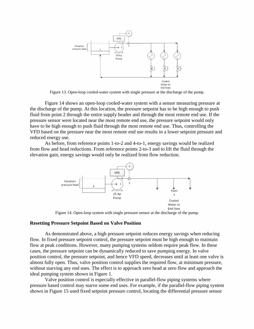
Figure 13. Open-loop cooled-water system with single pressure at the discharge of the pump.

Figure 14 shows an open-loop cooled-water system with a sensor measuring pressure at

the discharge of the pump. At this location, the pressure setpoint has to be high enough to push

fluid from point 2 through the entire supply header and through the most remote end use. If the

pressure sensor were located near the most remote end use, the pressure setpoint would only

have to be high enough to push fluid through the most remote end use. Thus, controlling the

VFD based on the pressure near the most remote end use results in a lower setpoint pressure and

reduced energy use.

As before, from reference points 1-to-2 and 4-to-1, energy savings would be realized

from flow and head reductions. From reference points 2-to-3 and to lift the fluid through the

elevation gain, energy savings would only be realized from flow reduction.

Figure 14. Open-loop system with single pressure sensor at the discharge of the pump.

Resetting Pressure Setpoint Based on Valve Position

As demonstrated above, a high pressure setpoint reduces energy savings when reducing

flow. In fixed pressure setpoint control, the pressure setpoint must be high enough to maintain

flow at peak conditions. However, many pumping systems seldom require peak flow. In these

cases, the pressure setpoint can be dynamically reduced to save pumping energy. In valve

position control, the pressure setpoint, and hence VFD speed, decreases until at least one valve is

almost fully open. Thus, valve position control supplies the required flow, at minimum pressure,

without starving any end uses. The effect is to approach zero head at zero flow and approach the

ideal pumping system shown in Figure 1.

Valve position control is especially effective in parallel-flow piping systems where

pressure based control may starve some end uses. For example, if the parallel-flow piping system

shown in Figure 15 used fixed setpoint pressure control, locating the differential pressure sensor

in circuit A may starve end uses in the circuit B if circuit B requires more flow and pressure than

circuit A. Valve position control is less effective on systems with multiple end uses of different

sizes. Moreover, valve position control does not set the lower limit on VFD speed; this is done

elsewhere in the control algorithm.

Figure 15. Parallel-flow pumping system.

CASE STUDY

The following case study demonstrates energy saving potential from minimizing bypass

flow and pressure control losses. The variable-flow HVAC chilled water system shown in

Figure 16 employs best practice by locating a differential pressure sensor near the most remote

end use. In addition, the pressure sensors across the chiller evaporators can be used to measure

flow through the evaporators to ensure minimum flow. The use of reverse return balances

unregulated flow through the air handlers (Taylor 2002). The use of a three-way bypass valve at

AHU 1 is not a recommended practice because some flow is always being pumped through the

bypass.

Figure 16. Chilled water pumping system in case study.

Despite the existence of VFDs and well-located pressure sensors, data from the control

system indicate non-optimal control. Figure 17 shows measured five-minute VFD speed versus

building differential pressure (dP) data from April 2014 to November 2014 when only Pump 1

was operating. Figure 18 shows measured five-minute VFD speed versus chiller evaporator dP

data from April 2014 to November 2014 when only Pump 1 was operating. In a properly

controlled system, the VFD should vary speed to maintain a constant building dP. However, the

data show that the building dP varies between 1 psi and 8 psi. In addition, in a properly

controlled system, the VFD speed and building dP should be highly correlated. However,

statistical analysis shows an R2 value of 0.02 between VFD speed and building dP. In fact, Pump

1 operates at 70% for 55% of the time. According to the chiller specification sheets, the chiller

evaporator dP must be between 1.4 psi and 6.4 psi. However, it maintains an average chiller

evaporator dP of 6 psi and often exceeds the limit of 6.4 psi. All this indicates very poor control.

Time series data offers more insight into the control problems. As seen in Figure 19, the

VFD operated at an average speed of 70% on Saturday, May 10, when the average outdoor air

temperature was 65.5 ˚F, the average relative humidity was 70% and occupancy and internal

loads were small. In Figure 20, the VFD operated at an average speed of 64% on Thursday, July

10, when the average outdoor air temperature was 70.7 ˚F1 and the average relative humidity was

66%2 and occupancy and internal loads were high. If properly controlled, the VFD speed would

be higher on a hotter, wetter day with higher occupancy and internal loads. However, the

opposite is true. The VFD speed is stuck at 70% on May 10 and drops to 30% on July 10. This

indicates inefficient control.

Figure 19. Trend data on Saturday, May 10, 2014. Figure 20. Trend data on Thursday, July 10, 2014.

1 Average daily temperatures were taken from Kissock’s Average Daily Temperature Archive:

http://academic.udayton.edu/kissock/http/Weather/ 2 Relative humidity taken from Weather Underground: http://www.wunderground.com

Figure 17. Building dP vs. VFD Speed. Figure 18. Chiller Evaporator dP vs. VFD Speed.

0

10

20

30

40

50

60

70

80

90

100

0 2 4 6 8 10

VSD

Sp

eed

(%

)

Building dP (psi)

Building differential pressure varies from 1 psi to 7.5 psi.

0

10

20

30

40

50

60

70

80

90

100

0 1 2 3 4 5 6 7 8V

FD S

pee

d (

%)

Evaporator dP (psi)

Upper limit of chiller evaporator dP, 6.4 psi

The original control algorithm executes the following steps:

1. Chiller 1 and Pump 1 turn on when the outdoor air temperature is above 65 ˚F. For

outdoor air temperatures between 55 ˚F and 65 ˚F, economizers on the air handling units

(AHU) are able to meet the cooling load.

2. Differential pressure is read across the building and Chiller 1 evaporator:

The chiller evaporator dP must be maintained between 1.5 psi and 6.4 psi. If it is

higher or lower, the VFD ramps up or down to maintain the upper and lower

bounds.

The building dP setpoint is 10 psi. The VFD simultaneously ramps up or down to

maintain 10 psi across the building.

3. If the building dP drops below 2.3 psi for 30 minutes, pump 2 turns on to increase

building pressure.

4. If the chilled water supply temperature is greater than 48 ˚F, Chiller 2 comes on to

provide more cooling capacity to the building.

Because of the 6.4 psi upper bound on the chiller evaporator dP, the VFD is always

hunting for, but never reaches, the building dP setpoint of 10 psi. To improve energy-efficiency,

the building dP setpoint should be reset to 2.3 psi. According to maintenance personnel this is

sufficient to supply all air handlers with adequate flow. In addition, it guarantees a minimum of

1.4 psi pressure drop, and minimum flow, through the evaporator. This change will stop the VFD

from hunting for a set-point it can never attain. Instead, the VFD speed will vary with the

thermal building load; resulting in better controlled and more energy-efficient pumping. Using

the pump affinity law with an exponent of 2.5, the estimated annual savings from implementing

the reduced building dP setpoint are 47% of chilled water pumping energy use.

After this change is successfully implemented, we will recommend replacing the 3-way

bypass valve with an actuated 2-way bypass valve controlled to provide a minimum pressure

drop, and hence flow, across the chiller evaporator. Next, we will recommend resetting the

building dP setpoint based on valve position. We will begin implementing these changes after

sufficient baseline data is collected so energy savings can be measured.

CONCLUSIONS

This paper describes several best practices for controlling variable-flow pumping

systems. As variable-flow pumping systems become more common, adhering to these best

practices are important in order to maximize energy savings. In our experience, many variable-

flow pumping systems are not optimally controlled, so the potential for savings is great.

To maximize energy savings in variable-flow pumping systems, bypass flow should be

minimized or eliminated. Best practice to eliminate excess bypass flow is to employ an actuated

two-way bypass valve or primary-secondary pumping. If the effect of excess bypass is neglected,

savings calculations will significantly overestimate savings.

Best practice in controlling VFD speed is locating a differential pressure sensor near the

most remote end use in the system. To increase energy savings, the dP setpoint should be as low

as possible. Further, valve position can be used to reset the pressure setpoint downward to allow

static head to approach zero and maximize energy savings.

ACKNOWLEDGMENTS

We are grateful for support for this work from the U.S. Department of Energy through

the Industrial Assessment Center program and through an Excellence in Applied Energy

Engineering Research grant. We are very grateful to Steve Kendig and John Brammer for

providing access to and information about the chilled water pumping system and for helping us

develop an improved algorithm. We are also grateful to Bernard Glascoe for assisting us in the

UDHL. We are also very grateful to Jeremy Fauber for technical support and feedback. Finally,

we are grateful to the IAC students and staff upon whose work this effort is built.

REFERENCES

ANSI/ASHRAE Standard 90.1-2010, Energy Standard for Buildings Except Low-Rise

Residential Buildings

Avery, Gil and Rishel, James B. 2009. "Case Against Balancing Valves." ASHRAE Journal 26-

29. ASHRAE, July.

Bernier and Bourret, 1999, “Pumping Energy and Variable Frequency Drives”, ASHRAE

Journal, December.

EERE (Energy Efficiency and Renewable Energy). 2001. “Pump Life Cycle Costs: A Guide to

LCC Analysis for Pumping Systems.” U.S. Department of Energy

https://www1.eere.energy.gov/manufacturing/tech_assistance/pdfs/pumplcc_1001.pdf

Grundfos Management. 2011. “All You Need to Know About Pumps and Energy”

http://energy.grundfos.com/en/facts-on-pumps-energy/energy-and-pump-facts

Kissock, J. 2014a. Energy Efficient Buildings: Duct System Design, CAV/VAV.

http://academic.udayton.edu/kissock/http/EEB/Energy%20Efficient%20Buildings_1.htm

Ma, Y., Turker, A., Kissock, J. 2015. “Energy Efficient Static Pressure Reset in VAV Systems.”

2015 ASHRAE Winter Conference, Chicago: ASHRAE.

Maxwell, Jonathan. 2005. “How to Avoid Overestimating Variable Speed Drive Savings.”

NCSU (North Carolina State University). 2014. DSIRE (Database of State Incentives for

Renewables & Energy Efficiency). www.dsireusa.org

Taylor, S., Stein, J. 2002. “Balancing Variable Flow Hydronic Systems.” ASHRAE Journal,

October.

Taylor, S. 2012. “Optimizing Design & Control of Chilled Water Plants, Part 5: Optimized

Control Sequences.” ASHRAE Journal, June.