Are Kalecki-Minsky models consistent with the data? Evidence

from the US

Alejandro Gonzalez∗

September 24, 2018

Abstract: Post-Keynesians have incorporated one or more insights from Minsky’s work in theirmacroeconomic models at an exponential rate during the past 10 years. The time to produce rigor-ous empirical work in order to discriminate the relevance of different families of models seems ripe.This paper contributes to filling this gap in the literature by estimating various forms of Kalecki-Minsky models for the US whose reduced-form representation are nested by linear and non-linearvector autoreggressions containing leverage and accumulation. The results imply that all modelsconsidered in the literature, except for the Charles model, are broadly inconsistent with the data.Many of the non-linear restrictions implied by the Charles model are borne by the data: There is alow leverage and a high leverage equilibrium and in both equilibria accumulation is debt burdened.However, we do not find evidence of increased financial instability in the high leverage equilibria, asproposed by the Charles model, nor do we find any evidence of the Financial Instability Hypothesisor the Paradox of Debt in any of the equilibria. This implies that much more work needs to bedone to understand the dynamic effects of leverage on accumulation, instead of focusing on modelswhich emphasize the univariate dynamics of leverage.

Key words: Kalecki-Minsky Models, Leverage, Vector Autoreggression, Non-Linear Time SeriesJEL codes: C32, E02, E12

PRELIMINARY DRAFT - PLEASE DO NOT CITE

∗Universidad de Chile. Mail: Agonzalezc@fen.uchile.cl. The author would like to thank Romulo Chumacero forhis guidance, patience and numerous discussion during the period of research that led to this paper. The authorwould also like to thank Matheus Grasselli, Francisco Diaz-Valdez, Rafael Ribeiro and Guilherme Magacho for theircomments and discussions on previous drafts of this paper, as well as participants in the INET 2017 conference.Finally, he would also like to thank Isidora Diaz for her assistance using the package tikz.

1

1 Introduction

Hyman Minsky’s (1975, 1982, 1986, 1992) prolific work regarding the financial dynamics of ma-ture capitalists economies has attracted renewed attention both from the mainstream press andheterodox authors since the sub-prime financial crisis. Accordingly, there has been an explosion inthe formalization of many Minskian insights into otherwise standard Kaleckian, Harrodian, Good-winian and Kaldorian macroeconomic models, a literature which has been recently surveyed byNikolaidi and Stockhammer (2017).1

Unfortunately, econometric work aimed at distinguishing the empirical plausibility of these differ-ent models is rather scarce, not to say non-existent. This paper aims to fill this empirical gap byinvestigating the empirical implications of Kalecki-Minsky models. We exploit the fact that mostmodels produced in the literature can be written either as a two dimensional dynamical systemon leverage and output or as one dimensional dynamical systems on leverage. This implies thatlinear and non-linear vector autorregressions (VAR) nest these models as special cases. Indeed, alinear univariate autoregressive model of leverage is implied by the model of Hein (2007), a non-linear univariate autoregressive model is implied by the models described in Taylor (2009), Lavoie(1995;2014), which is examined in depth in Ryoo (2013a), and a non-linear VAR on accumulationand leverage is implied by the more sophisticated Kaleckian model of Charles (2008a).2

The few existing empirical investigations regarding Minsky’s ideas are not explicitly derived from aheterodox macroeconomic model, and thus, are poorly suited to try to discriminate between com-peting frameworks in which to understand Minsky’s work. There are two exceptions to this rule.The first exception concerns the study by Nishi (2012), where the author claims that he developsa discrete-time version of Charles (2008a) Kalecki-Minsky model, and develops some identifyingrestrictions for a three-dimensional Vector Autoreggresion (VAR) on accumulation, leverage, andthe profit share. The author’s main finding is that the Japanese economy exhibits a debt-burdenedand profit-led accumulation rate, while the leverage rate is essentially insensitive to accumulationand distribution. While this paper is an important contribution to the literature, it suffers from twoflaws: As we discuss later, the paper does not implement the Charles model in the correct fashion,since it uses a linear specification for a non-linear model. Secondly, the paper does not discuss howhis findings help to either accept or reject Kalecki-Minsky models or their broader implications forthe theoretical literature which seeks to model Minsky.

The second exception to this rule is the small literature which has discussed Minsky’s financialinstability hypothesis (FIH), which has been mostly interpreted as the idea that business cyclesshould exhibit pro cyclical leverage. The FIH is typically a building block in Minskian models,since it specifies the dynamic response of leverage to output or accumulation. The first and mostinfluential attempt at testing this question is conducted in Lavoie and Seccareccia (2001), wherethe authors analyse the correlation between GDP and the aggregate debt to equity ratio for six

1Lavoie (2009) provides a comprehensive review on the earlier literature, although in the context of the evolutionof Cambridge Post-Keynesians and American Fundamentalists Keynesians.

2Of course, as underlined by Nikolaidi and Stockhammer (2017), the modelling of leverage and accumulation isnot the only way to formalize Minsky’s views. Other Kaleckian formalizations stress the role of interest rate dynamics(Lima and Meirelles, 2007; Fazzari, Ferri and Greenberg, 2008) or the dynamics of the retention ratio set by firms(Charles, 2008b). Also, a smaller but growing literature analyses the roles of asset prices and their interaction withgoods market to produce instability and Minsky cycles; see, for example, Ryoo (2013b). However, it seems fair tosay that most Kaleckian models have emphasized the leverage - output link as an accurate interpretation of manymajor Minskian insights, so we postpone an empirical investigation of these families of models for the future.

2

OECD countries at yearly frequencies. They essentially conclude that the leverage rate is a-cyclical.Furthermore, they estimate a regression of leverage on GDP growth, noting that economic activityis not significant once appropriate controls are included, with the point estimates always displayinga negative coefficient. This would imply that leverage and GDP are counter-cyclical, a phenom-ena professor Lavoie would latter name ’The paradox of debt’: Firms attempt to cut debt duringrecessions would further depress economic activity, which would conduce to higher leverage ratiosduring recessions and lower leverage ratios during expansions. As mentioned above, this finding isessentially corroborated by Nishi for Japan.

However, there has also been some evidence contradicting the Paradox of Debt and supporting theFIH. A few representative examples are Charles (2015) and Gonzalez and Perez-Caldentey (2017):While the first paper shows that are low frequency comovements between GDP and aggregate lever-age3 over the 20th century in the US economy, the second paper shows that for a panel of firms in12 Latin American countries the paradox of debt is rejected in favour of the FIH. These authorsalso show that there is an important asymmetry regarding the FIH: the correlation between debtand investment is higher during expansions than during recessions.4

The main results of our empirical investigation are summarized as follows: First, linear Kalecki-Minsky models, such as the one proposed by Hein (2007), are broadly inconsistent with the data. Alinear specification reveals there is no feedback effect whatsoever from leverage to accumulation andfrom accumulation to leverage. Furthermore, there is substantial evidence of non-linearities in theleverage series. Second, models which are solved in terms of a univariate specification of leverageare also broadly inconsistent with the data. They do not predict the correct number of equilibriaempirically nor do they characterize the qualitative behaviour of these equilibria in the correctfashion. Thirdly, the Charles (2008a) model seems to be the most promising candidate to explainthe features of our dataset: It correctly predicts the existence of two equilibria - a low leverage equi-libria and a high leverage equilibria, and also correctly predicts that accumulation is debt-burdenedin this two equilibria. However, it incorrectly characterizes the low leverage equilibria as stable andthe high leverage equilibria as unstable. The equilibria estimated in the data present exactly theopposite features: The low-leverage equilibria is stationary while the high-leverage equilibria showsunit-root like behaviour. Furthermore, leverage does not react to lagged accumulation in eitherof the equilibria, implying that neither the FIH or the Paradox of debt hold in any regime. Allin all, while the Charles model fails to explain some important patterns of the data, many of itsinteresting properties are borne out in our dataset. Thus, further work in the Kaleckian traditionneeds to be directed at analysing the dynamic feedbacks from leverage to the goods market, and lesstime needs to be devoted on models whose emphasis is solely on the univariate dynamics of leverage.

This paper is organized as follows: Section 2 briefly reviews a series of Kalecki-Minsky models,paying special attention to the dynamical systems that describe the evolution of the economy overtime. Section 3 presents our data sources, with special care of our definition of Aggregate Debt, andsome stylized facts of our univariate series. Section 4 starts by tracing the empirical implicationsof the various vintages of Kaleckian models presented earlier. It then proceeds to show how vectorauto regressions can be used to test these implications. Section 5 presents our main results, wherethe number and qualitative properties of the equilibria present in the data are analysed. Section 6

3The aggregate leverage ratio is measured as the debt to GDP ratio4Evidently, other empirical work exists, such as Isenberg (1988) or more recently, Davis, de Souza and Hernandez

(2017). This article claims that this rich empirical work either doesn’t nest or doesn’t test an explicit macroeconomicmodel.

3

presents some last remarks on the Minsky research agenda and concludes.

2 Minsky’s insights in a Kaleckian framework.

As noted by Nikolaidi and Stockhammer (2017), there has been an explosion of formal presenta-tions of Minsky’s insights during the last decade. Many differences stand out across these models:Among them, the choice of endogenous variables, the focus on cycles or explosive instability, andtheir use of different heterodox authors to complement Minsky’s work.

However, it seems fair to say that extensions of the benchmark Neo-Kaleckian model, presentedin texbook form in Lavoie (2014) and Hein (2014), for example, are one of the most popular waysto formalize Minsky’s work. This section starts presenting the Kalecki-Minsky model of Charles(2008a), and then shows how successive simplifying assumptions yield different models popular inthe literature.

2.1 Model 1: Sluggish adjustment in the goods market

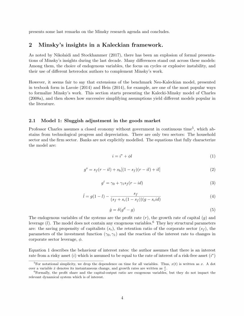
Professor Charles assumes a closed economy without government in continuous time5, which ab-stains from technological progress and depreciation. There are only two sectors: The householdsector and the firm sector. Banks are not explicitly modelled. The equations that fully characterizethe model are:

i = i∗ + φl (1)

gs = sf (r − il) + sh[(1− sf )(r − il) + il] (2)

gi = γ0 + γ1sf (r − id) (3)

l = g(1− l)− sf(sf + sc(1− sf ))(g − scid)

(4)

g = δ(gd − g) (5)

The endogenous variables of the systems are the profit rate (r), the growth rate of capital (g) andleverage (l). The model does not contain any exogenous variables.6 They key structural parametersare: the saving propensity of capitalists (sc), the retention ratio of the corporate sector (sf ), theparameters of the investment function (γ0, γ1) and the reaction of the interest rate to changes incorporate sector leverage, φ.

Equation 1 describes the behaviour of interest rates: the author assumes that there is an interestrate from a risky asset (i) which is assumed to be equal to the rate of interest of a risk-free asset (i∗)

5For notational simplicity, we drop the dependence on time for all variables. Thus, x(t) is written as x. A dotover a variable x denotes its instantaneous change, and growth rates are written as x

x.

6Formally, the profit share and the capital-output ratio are exogenous variables, but they do not impact therelevant dynamical system which is of interest.

4

plus a risk premium associated with the level of leverage of the corporate sector.7 The rationalefor this equation is Kalecki’s (1937) principle of increasing risk.

Equations 2, 3 and 5 characterize the behavior of the goods market: The growth rate of savings (2)is decomposed in savings from the corporate sector, which retain a constant fraction (sf ) of theirretained earnings (r− il), and the household sector, in which only capitalists save a constant frac-tion of their dividend income, and their rentier income. The growth rate of investment is a functionsolely of retained earnings and a constant. Finally, equation 5 assumes that actual accumulationadjusts slowly to the desired by capitalists.8

Equation 4 is obtained by assuming that investment can only be financed by means of retainedearnings or by issuing debt9; thus, equity finance plays no role in this model. As mentioned be-fore, since internal finance is simply a fraction of retained earnings, debt grows to close the gapbetween desired investment and internal finance, bearing all of the adjustment in the firm’s budgetconstraint.

The model is closed by assuming that savings (2) must be equal to actual accumulation, andplugging desired investment (3) into the adjustment equation (5). Replacing the interest rateequation into the investment function gives a two-dimensional dynamical system in leverage andaccumulation which is quadratic:

g = a1 + a2g − a3l − a4l2 (6)

l = b1g − b2gl + b3l + b4l2 (7)

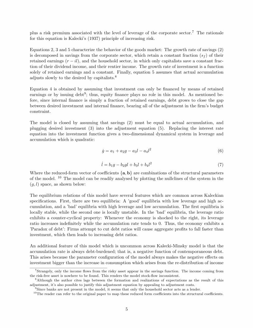
Where the reduced-form vector of coefficients {a,b} are combinations of the structural parametersof the model. 10 The model can be readily analysed by plotting the nullclines of the system in the(g, l) space, as shown below:

The equilibrium relations of this model have several features which are common across Kaleckianspecifications. First, there are two equilibria: A ’good’ equilibria with low leverage and high ac-cumulation, and a ’bad’ equilibria with high leverage and low accumulation. The first equilibria islocally stable, while the second one is locally unstable. In the ’bad’ equilibria, the leverage ratioexhibits a counter-cyclical property: Whenever the economy is shocked to the right, its leverageratio increases indefinitely while the accumulation rate tends to 0. Thus, the economy exhibits a’Paradox of debt’: Firms attempt to cut debt ratios will cause aggregate profits to fall faster thaninvestment, which then leads to increasing debt ratios.

An additional feature of this model which is uncommon across Kalecki-Minsky model is that theaccumulation rate is always debt-burdened; that is, a negative function of contemporaneous debt.This arises because the parameter configuration of the model always makes the negative effects oninvestment bigger than the increase in consumption which arises from the re-distribution of income

7Strangely, only the income flows from the risky asset appear in the savings function. The income coming fromthe risk-free asset is nowhere to be found. This renders the model stock-flow inconsistent.

8Although the author cites lags between the formation and realizations of expectations as the result of thisadjustment, it’s also possible to justify this adjustment equation by appealing to adjustment costs.

9Since banks are not present in the model, it seems that only the household sector acts as a lender.10The reader can refer to the original paper to map these reduced form coefficients into the structural coefficients.

5

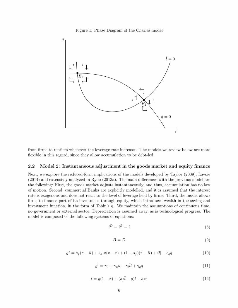
Figure 1: Phase Diagram of the Charles model

l

g

l = 0

E1

E2

g = 0

from firms to rentiers whenever the leverage rate increases. The models we review below are moreflexible in this regard, since they allow accumulation to be debt-led.

2.2 Model 2: Instantaneous adjustment in the goods market and equity finance

Next, we explore the reduced-form implications of the models developed by Taylor (2009), Lavoie(2014) and extensivly analyzed in Ryoo (2013a). The main differences with the previous model arethe following: First, the goods market adjusts instantaneously, and thus, accumulation has no lawof motion. Second, commercial Banks are explicitly modelled, and it is assumed that the interestrate is exogenous and does not react to the level of leverage held by firms. Third, the model allowsfirms to finance part of its investment through equity, which introduces wealth in the saving andinvestment function, in the form of Tobin’s q. We maintain the assumptions of continuous time,no government or external sector. Depreciation is assumed away, as is technological progress. Themodel is composed of the following systems of equations:

iD = iB = i (8)

B = D (9)

gs = sf (r − il) + sh[u(v − r) + (1− sf )(r − il) + il]− cqq (10)

gi = γ0 + γuu− γl il + γqq (11)

l = g(1− x) + (sf i− g)l − sfr (12)

6

Compared with the previous model, the utilization rate is introduced as an endogenous variablewhich adjusts to clear the goods market, which is a defining characteristic of Kaleckian models.The model now has three exogenous variables: the capital to potential output ratio (v), the profitshare (π) and the interest rate (i). They key structural parameters are: the saving propensityof the household sector (sh), the retention ratio of the corporate sector (sf ), the percentage ofinvestment financed by equities, (x), the parameters of the investment function (γ0, γu, γl, γq), andthe propensities to consume out of wealth, cq.

Equations (8) and (9) describe the behaviour of banks: The interest rate on deposits is set equalto the interest rate on loans, which is exogenous. Additionally, since it is assumed that the publicdoes not hold money and that banks don’t hold reserves, bank loans (B) are equal to bank deposits(D).

Equation (10) now assumes that workers do save as a class, and thus we analyse the savings of thehousehold sector as a whole via the parameter sc. It is also know assumed that there are somewealth effects from consumption, contained into Tobin’s q. Equations (11) and (12) describe thebehaviour of the firm: Investment now additionally depends on the utilization rate and Tobin’s q.Retained earnings now do not appear as a determinant of investment; only interest payments outof debt.11 The differential equation for leverage is derived from the finance frontier of the firm,which states that the growth of investment expenditures net of wage payments must be financedeither by issuing equities, bank loans or retained earnings. As mentioned before, equation (12) isextended to include the fact that equity finance is a fixed percentage of investment, while internalfunds enter the finance frontier in the same way.

Long-run equilibrium requires that the goods market clears in every period (which implies (10)= (11)), and that investment expenditures are consistent with the budget constraint of the firm(which implies (11) = (12)). It is assumed that the utilization rate adjusts to clear the goodsmarket, while leverage adjusts to bring in planned investment in line with the budget constraintof the firm. Since only leverage exhibits dynamic behaviour, however, the whole economy can becharacterized by solving the dynamics of leverage: we can obtain the trajectories of the growth rateof capital, the profit rate and the utilization rate all as functions of leverage.

Thus, if we denote g(l) as the equilibrium growth rate of capital as a function of leverage, which isderived from the equilibrium on the goods market, equation (12) becomes:

l = g(l)(1− x) + (sf i− g(l))l − sfr (13)

It can be shown that g(l) is a linear function of leverage, which implies that (7) will be a quadraticfunction of leverage. The reaction of the goods market to leverage will be crucial to determiningequilibrium: if the goods market is ’debt-led’(g′(l) > 0), the quadratic equation will have onlyone equilibrium with positive leverage, which will be globally stable. If the goods market is ’debt-burdened’, (g′(l) < 0), the above equation will have two equilibiria: One with low leverage andhigh growth, which will be locally stable, and one with high leverage and low growth, which willbe locally unstable.12 Figure 2 plots the phase line for both cases.

11Thus, in this variant of the Kalecki-Minsky models, it’s not clear what explains the impact of interest paymentsof investment, since if a cash-constrained story would hold, we would expect the profit rate to enter the investmentfunction with the same parameter value as interest payment, as in the Charles model.

12See Ryoo (2013), pages 6-7 for a more detailed discussion of these results.

7

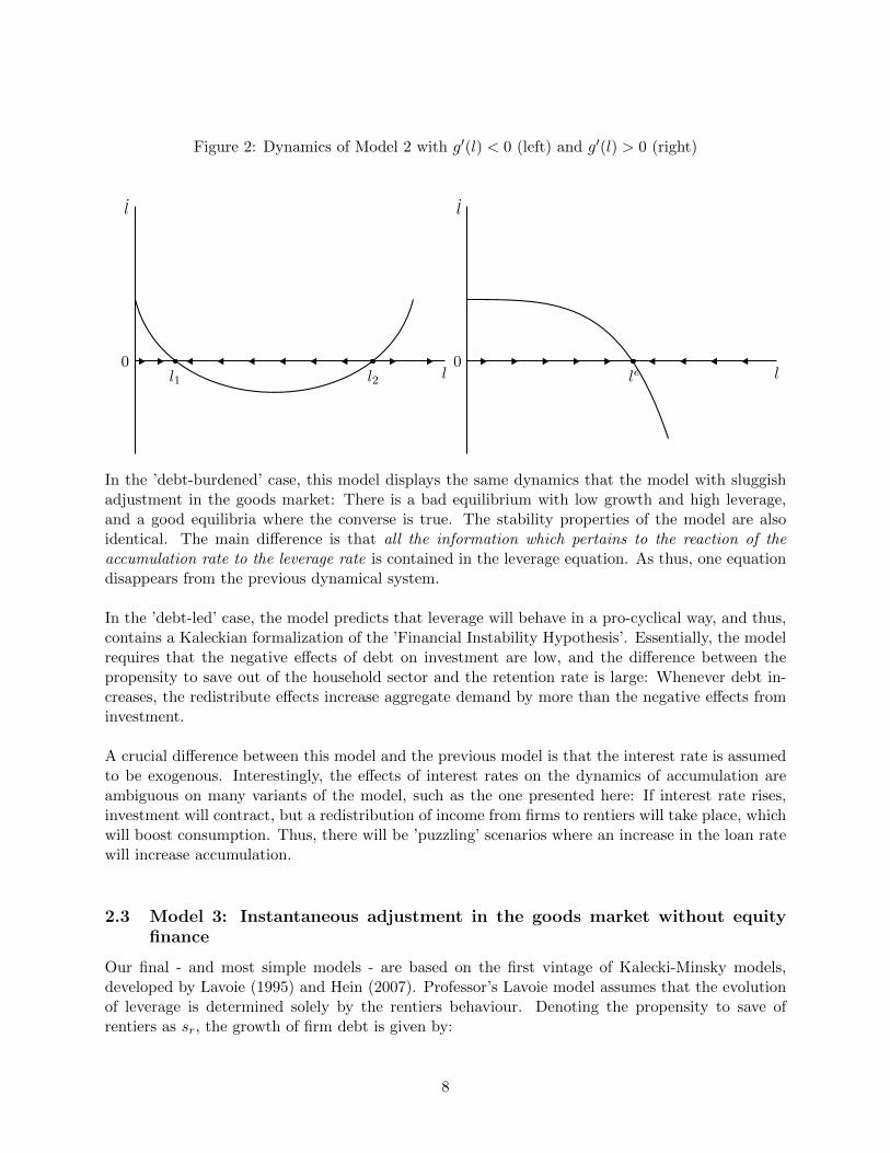
Figure 2: Dynamics of Model 2 with g′(l) < 0 (left) and g′(l) > 0 (right)

l

l

0l1 l2 l

l

0le

In the ’debt-burdened’ case, this model displays the same dynamics that the model with sluggishadjustment in the goods market: There is a bad equilibrium with low growth and high leverage,and a good equilibria where the converse is true. The stability properties of the model are alsoidentical. The main difference is that all the information which pertains to the reaction of theaccumulation rate to the leverage rate is contained in the leverage equation. As thus, one equationdisappears from the previous dynamical system.

In the ’debt-led’ case, the model predicts that leverage will behave in a pro-cyclical way, and thus,contains a Kaleckian formalization of the ’Financial Instability Hypothesis’. Essentially, the modelrequires that the negative effects of debt on investment are low, and the difference between thepropensity to save out of the household sector and the retention rate is large: Whenever debt in-creases, the redistribute effects increase aggregate demand by more than the negative effects frominvestment.

A crucial difference between this model and the previous model is that the interest rate is assumedto be exogenous. Interestingly, the effects of interest rates on the dynamics of accumulation areambiguous on many variants of the model, such as the one presented here: If interest rate rises,investment will contract, but a redistribution of income from firms to rentiers will take place, whichwill boost consumption. Thus, there will be ’puzzling’ scenarios where an increase in the loan ratewill increase accumulation.

2.3 Model 3: Instantaneous adjustment in the goods market without equityfinance

Our final - and most simple models - are based on the first vintage of Kalecki-Minsky models,developed by Lavoie (1995) and Hein (2007). Professor’s Lavoie model assumes that the evolutionof leverage is determined solely by the rentiers behaviour. Denoting the propensity to save ofrentiers as sr, the growth of firm debt is given by:

8

l = [srr − g(l)]l (14)

As before, two equilibria exists with the same characteristics as the previous model. Thus, we deferto commenting it further. Professor’s Hein model is the simplest model of the ones consideredhere: There is istantaneous adjustment in the goods market, workers do not save, dividends are notdistributed (sf = 1), there are no equities in the model, and a class of pure rentiers exists whichsaves in the form of deposits. The growth rate of leverage is thus a simplified version of (12) whichequals:

l = g − (1− l)r (15)

The linearity of the leverage function now guarantees the existence of only one steady state whetherthe accumulation rate is debt-led or debt-burdened. However, the debt-led regime will be globallystable, and the debt-burdened regime will be globally unstable.

To summarize our discussion, various Kalecki-Minsky models imply a dynamical system which ex-hibits multiple equilibria. In general, the high leverage equilibria will be unstable, while the lowleverage equilibria is stable. These multiple equilibria can arise either from specific assumptionsregarding how firm’s finance investment - specifically, assuming that equity finance is a fixed pro-portion of investment, or by assuming that the risk premium is a function of leverage. We willdiscuss how to test these and other implications below; however, we first turn to discussions relatedto data sources.

3 Data Sources and Stylized Facts

In order to appropriately estimate the Kaleckian-Minsky model outlined above, we need two rele-vant time series. The first one concerns the accumulation rate, while the second one concerns themeasure of leverage employed in the model. Unfortunately, previous empirical work has not beenconsistent when measuring leverage. Lavoie and Secareccia (2001) use a measure of debt securitiesover equity, while Charles (2008) uses a measure of aggregate debt over GDP. However, the Kaleck-ian model employs aggregate bank loans over tangible capital as its relevant measure of leverage.Thus, in order to stay as closely as possible to our theoretical model, we attempt to construct atime series consistent with this notion.

We first obtain our series of annual capital stock as the current-cost gross stock of private fixedassets constructed by the Bureau of Economic Analysis. This constitutes the denominator of ourseries. The numerator of our series should be a measure of aggregate debt. If we were to takeour model literally, this measure should only contain aggregate bank loans of the corporate andnon-corporate financial sector, which is readily available from the flow of funds accounts. However,one could also argue that one should not take this simplification literally and should add otherdebt securities used by the corporate sector, such as corporate bonds, mortgages, and so on. Wechoose to employ this latter measure of aggregate debt. The capital accumulation series is simplyconstructed by taking total investment in fixed assets by the private sector and dividing them byour measure of the capital stock. All series are measured in real terms.13

13Links to all data sources.

9

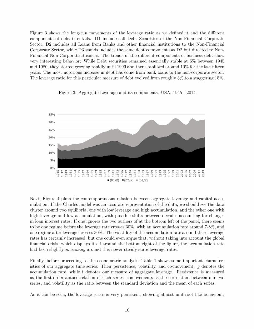
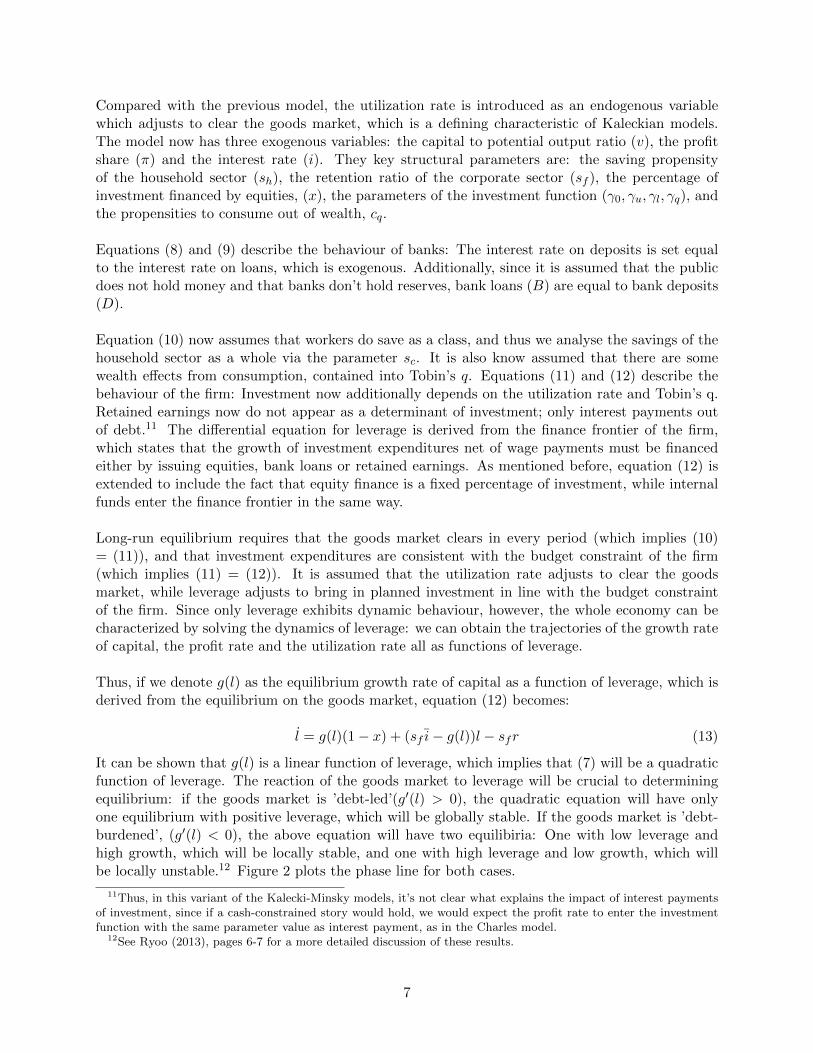
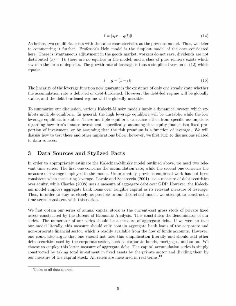
Figure 3 shows the long-run movements of the leverage ratio as we defined it and the differentcomponents of debt it entails. D1 includes all Debt Securities of the Non-Financial CorporateSector, D2 includes all Loans from Banks and other financial institutions to the Non-FinancialCorporate Sector, while D3 stands includes the same debt components as D2 but directed to Non-Financial Non-Corporate Business. The trends of the different components of business debt showvery interesting behavior: While Debt securities remained essentially stable at 5% between 1945and 1980, they started growing rapidly until 1999 and then stabilized around 10% for the last fifteenyears. The most notorious increase in debt has come from bank loans to the non-corporate sector.The leverage ratio for this particular measure of debt evolved from roughly 3% to a staggering 15%.

Figure 3: Aggregate Leverage and its components. USA, 1945 - 2014

0%

5%

10%

15%

20%

25%

30%

35%

1945

1947

1949

1951

1953

1955

1957

1959

1961

1963

1965

1967

1969

1971

1973

1975

1977

1979

1981

1983

1985

1987

1989

1991

1993

1995

1997

1999

2001

2003

2005

2007

2009

2011

2013

(D1/K) (D2/K) (D3/K)

Next, Figure 4 plots the contemporaneous relation between aggregate leverage and capital accu-mulation. If the Charles model was an accurate representation of the data, we should see the datacluster around two equilibria, one with low leverage and high accumulation, and the other one withhigh leverage and low accumulation, with possible shifts between decades accounting for changesin loan interest rates. If one ignores the two outliers of at the bottom left of the panel, there seemsto be one regime before the leverage rate crosses 30%, with an accumulation rate around 7-8%, andone regime after leverage crosses 30%. The volatility of the accumulation rate around these leveragerates has certainly increased, but one could even argue that, without taking into account the globalfinancial crisis, which displays itself around the bottom-right of the figure, the accumulation ratehad been slightly increasing around this newer steady-state leverage rates.

Finally, before proceeding to the econometric analysis, Table 1 shows some important character-istics of our aggregate time series: Their persistence, volatility, and co-movement. g denotes theaccumulation rate, while l denotes our measure of aggregate leverage. Persistence is measuredas the first-order autocorrelation of each series, comovements as the correlation between our twoseries, and volatility as the ratio between the standard deviation and the mean of each series.

As it can be seen, the leverage series is very persistent, showing almost unit-root like behaviour,

10

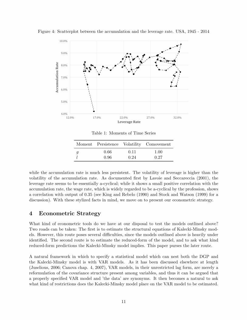
Figure 4: Scatterplot between the accumulation and the leverage rate. USA, 1945 - 2014

4.0%

5.0%

6.0%

7.0%

8.0%

9.0%

10.0%

12.0% 17.0% 22.0% 27.0% 32.0%

AccumulationRate

Leverage Rate

Table 1: Moments of Time Series

Moment Persistence Volatility Comovement

g 0.66 0.11 1.00l 0.96 0.24 0.27

while the accumulation rate is much less persistent. The volatility of leverage is higher than thevolatility of the accumulation rate. As documented first by Lavoie and Seccareccia (2001), theleverage rate seems to be essentially a-cyclical; while it shows a small positive correlation with theaccumulation rate, the wage rate, which is widely regarded to be a-cyclical by the profession, showsa correlation with output of 0.35 (see King and Rebelo (1990) and Stock and Watson (1999) for adiscussion). With these stylized facts in mind, we move on to present our econometric strategy.

4 Econometric Strategy

What kind of econometric tools do we have at our disposal to test the models outlined above?Two roads can be taken: The first is to estimate the structural equations of Kalecki-Minsky mod-els. However, this route poses several difficulties, since the models outlined above is heavily underidentified. The second route is to estimate the reduced-form of the model, and to ask what kindreduced-form predictions the Kalecki-Minsky model implies. This paper purses the later route.

A natural framework in which to specify a statistical model which can nest both the DGP andthe Kalecki-Minsky model is with VAR models. As it has been discussed elsewhere at length(Juselious, 2006; Canova chap. 4, 2007), VAR models, in their unrestricted lag form, are merely areformulation of the covariance structure present among variables, and thus it can be argued thata properly specified VAR model and ’the data’ are synonyms. It then becomes a natural to askwhat kind of restrictions does the Kalecki-Minsky model place on the VAR model to be estimated.

11

4.1 Testable Implications

Fortunately, variants of Kalecki-Minsky models are rich with implications. One common feature ofall the models explored above, with the sole exception of Hein (2007) is that these models featuremultiple equilibria: there is typically an bad equilibria with low growth and high leverage, and agood equilibria with the opposite characteristics. To fix ideas as to how this multiple-equilibriamight be tested in this setting, let us reproduce graphically the dynamics of leverage from model2 in the debt-burdened case, but in discrete time.

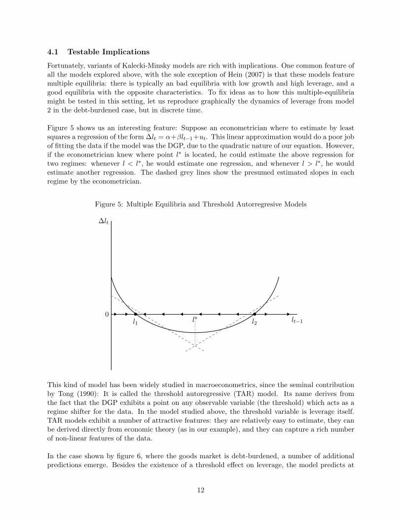
Figure 5 shows us an interesting feature: Suppose an econometrician where to estimate by leastsquares a regression of the form ∆lt = α+βlt−1+ut. This linear approximation would do a poor jobof fitting the data if the model was the DGP, due to the quadratic nature of our equation. However,if the econometrician knew where point l∗ is located, he could estimate the above regression fortwo regimes: whenever l < l∗, he would estimate one regression, and whenever l > l∗, he wouldestimate another regression. The dashed grey lines show the presumed estimated slopes in eachregime by the econometrician.

Figure 5: Multiple Equilibria and Threshold Autorregresive Models

lt−1

∆lt

0l1 l2l∗

This kind of model has been widely studied in macroeconometrics, since the seminal contributionby Tong (1990): It is called the threshold autoregressive (TAR) model. Its name derives fromthe fact that the DGP exhibits a point on any observable variable (the threshold) which acts as aregime shifter for the data. In the model studied above, the threshold variable is leverage itself.TAR models exhibit a number of attractive features: they are relatively easy to estimate, they canbe derived directly from economic theory (as in our example), and they can capture a rich numberof non-linear features of the data.

In the case shown by figure 6, where the goods market is debt-burdened, a number of additionalpredictions emerge. Besides the existence of a threshold effect on leverage, the model predicts at

12

most two distinct regimes, with each regime having distinct time series properties. The regime withlow leverage was shown to be locally stable, which implies that leverage should be stationary in thisregime, while the regime with high leverage is locally unstable, which means that leverage shouldbe non-stationary in this regime. Furthermore, the (sum of) coefficient(s) on the autorregresiveterms should change signs with each regime. Finally, we should expect to see a debt-burdenedgoods market: capital accumulation should react negatively to leverage in order to observe such anon-linearity.

It can be shown that all of these results carry on to the Charles model.14 The key additionalprediction of the Charles model is that the debt-burdened demand effects on accumulation havedynamic implications; that is, past values of leverage should also enter the accumulation rate. Thesluggish goods-market assumption guarantees that this holds, and this generates a two-dimensionaldynamical system which in turns implies a Threshold Vector Autorregression (TVAR) with the rateof growth of capital and leverage as endogenous variables. As before, the threshold variable shouldbe leverage, not accumulation; there should be at most 2 regimes, one regime with low leverageand high growth, and one regime with high leverage and low growth. The first regime should bestationary, while the second should be non-stationary, the autoregressive coefficient on the leverageequation should change signs when we change from one regime to another and finally, as before,these qualitative features of the data should be accompanied by a debt-burdened accumulation rateon each equilibrium.

4.2 Vector Autorregressions

In light of the above discussion, it seems fair to say that a one way to test the implications of theKalecki-Minsky model would imply the following steps: First, estimate the following linear VAR(p)model:

yt = c+A1yt−1 + ...+Apyt−p + ut (16)

Where yt = (lt, gt) is our vector time series containing leverage and accumulation, c is the vectorof constants, Ai is the matrix accompanying the i lagged vector of dependent variables and ut is avector of white noise shocks on each equation. Provided that our VAR passes the relevant diagnosticmisspecification tests, we could claim that we can pit the best linear approximation of the dataagainst a global linear alternative. If we reject the assumption of linearity, we would expect thenon-linearity to take a threshold form and the threshold variable to be leverage or lagged values ofleverage, but not the accumulation rate. In this case, the above model would take the form:

yt =

{c1 +A1

1yt−1 + ...+A1pyt−p + ut1 if lt−d ≤ l∗

c2 +A21yt−1 + ...+A2

pyt−p + ut2 if lt−d > l∗

Where l∗ is the threshold level of leverage, which we must estimate. With this formulation esti-mated, we can investigate whether the predictions outlined in the section above are fulfilled by ourTVAR model. This requires a few distinct steps; first, we need to test the existence of a thresholdeffect; second, we need to develop a method to distinguish which is the threshold variable, and

14One might suspect that the threshold variable in the Charles model is the accumulation rate; however, given thelogical bounds which must be imposed on a number of parameters, the non-linearity of the accumulation nullclinewill be generally much less pronounced that the one from the leverage nullcline. This makes us suspect that leveragewill also be the threshold variable in the Charles model.

13

to estimate its location; finally, we need to estimate the VAR model within each regime. Detailsregarding all of these issues as well as a review of influential applications of TAR and TVAR modelsare surveyed in Hansen (2010) and Hubrich and Terasvirta (2013).

5 Results

5.1 A linear VAR benchmark

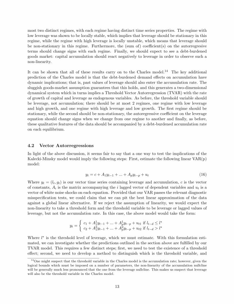
The first step towards specifying a linear VAR model is to select the maximum lag order, k. In orderto do so, we compute different information criteria for up two 5 lags. The results are presentedin Table 2. The results of this procedure are encouraging since all lag selection criteria suggest aVAR(2) model.15

Table 2: Lag-Length selection criteria

Lag AIC BIC HQ

1 -15.01 -14.81 -14.932 -15.67 -15.33 -15.543 -15.66 -15.19 -15.474 -15.57 -14.96 -15.335 -15.46 -14.73 -15.17

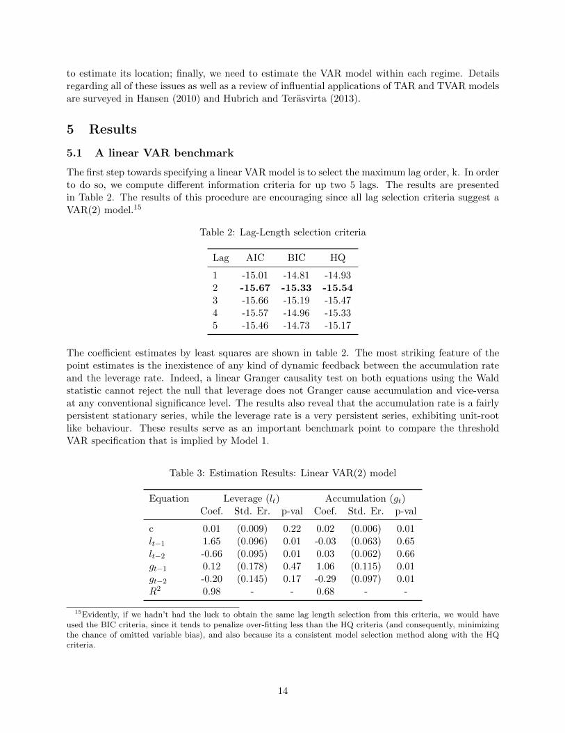
The coefficient estimates by least squares are shown in table 2. The most striking feature of thepoint estimates is the inexistence of any kind of dynamic feedback between the accumulation rateand the leverage rate. Indeed, a linear Granger causality test on both equations using the Waldstatistic cannot reject the null that leverage does not Granger cause accumulation and vice-versaat any conventional significance level. The results also reveal that the accumulation rate is a fairlypersistent stationary series, while the leverage rate is a very persistent series, exhibiting unit-rootlike behaviour. These results serve as an important benchmark point to compare the thresholdVAR specification that is implied by Model 1.

Table 3: Estimation Results: Linear VAR(2) model

Equation Leverage (lt) Accumulation (gt)Coef. Std. Er. p-val Coef. Std. Er. p-val

c 0.01 (0.009) 0.22 0.02 (0.006) 0.01lt−1 1.65 (0.096) 0.01 -0.03 (0.063) 0.65lt−2 -0.66 (0.095) 0.01 0.03 (0.062) 0.66gt−1 0.12 (0.178) 0.47 1.06 (0.115) 0.01gt−2 -0.20 (0.145) 0.17 -0.29 (0.097) 0.01R2 0.98 - - 0.68 - -

15Evidently, if we hadn’t had the luck to obtain the same lag length selection from this criteria, we would haveused the BIC criteria, since it tends to penalize over-fitting less than the HQ criteria (and consequently, minimizingthe chance of omitted variable bias), and also because its a consistent model selection method along with the HQcriteria.

14

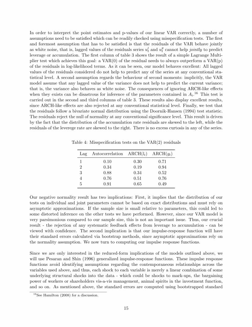
In order to interpret the point estimates and p-values of our linear VAR correctly, a number ofassumptions need to be satisfied which can be readily checked using misspecification tests. The firstand foremost assumption that has to be satisfied is that the residuals of the VAR behave jointlyas white noise, that is, lagged values of the residuals series ult and ugt cannot help jointly to predictleverage or accumulation. The first column of table 3 shows the result of a simple Lagrange Multi-plier test which achieves this goal: a VAR(0) of the residual needs to always outperform a VAR(p)of the residuals in log-likelihood terms. As it can be seen, our model behaves excellent: All laggedvalues of the residuals considered do not help to predict any of the series at any conventional sta-tistical level. A second assumption regards the behaviour of second moments: implicitly, the VARmodel assume that any lagged value of the variance does not help to predict the current variance;that is, the variance also behaves as white noise. The consequences of ignoring ARCH-like effectswhen they exists can be disastrous for inference of the parameters contained in Ai.

16 This test iscarried out in the second and third columns of table 3. These results also display excellent results,since ARCH-like effects are also rejected at any conventional statistical level. Finally, we test thatthe residuals follow a bivariate normal distribution using the Doornik-Hansen (1994) test statistic.The residuals reject the null of normality at any conventional significance level. This result is drivenby the fact that the distribution of the accumulation rate residuals are skewed to the left, while theresiduals of the leverege rate are skewed to the right. There is no excess curtosis in any of the series.

Table 4: Misspecification tests on the VAR(2) residuals

Lag Autocorrelation ARCH(lt) ARCH(gt)

1 0.10 0.30 0.712 0.34 0.19 0.943 0.88 0.34 0.524 0.76 0.51 0.765 0.91 0.65 0.49

Our negative normality result has two implications: First, it implies that the distribution of ourtests on individual and joint parameters cannot be based on exact distributions and must rely onasymptotic approximations. If the sample size is small relative to parameters, this could led tosome distorted inference on the other tests we have performed. However, since our VAR model isvery parsimonious compared to our sample size, this is not an important issue. Thus, our crucialresult - the rejection of any systematic feedback effects from leverage to accumulation - can beviewed with confidence. The second implication is that our impulse-response function will havetheir standard errors calculated via bootstrap methods, since asymptotic approximations rely onthe normality assumption. We now turn to computing our impulse response functions.

Since we are only interested in the reduced-form implications of the models outlined above, wewill use Pesaran and Shin (1996) generalized impulse-response functions. These impulse responsefunctions avoid identifying assumptions regarding the contemporaneous relationships across thevariables used above, and thus, each shock to each variable is merely a linear combination of someunderlying structural shocks into the data - which could be shocks to mark-ups, the bargainingpower of workers or shareholders vis-a-vis management, animal spirits in the investment function,and so on. As mentioned above, the standard errors are computed using bootstrapped standard

16See Hamilton (2008) for a discussion.

15

errors which are drawn from 1000 repetitions.

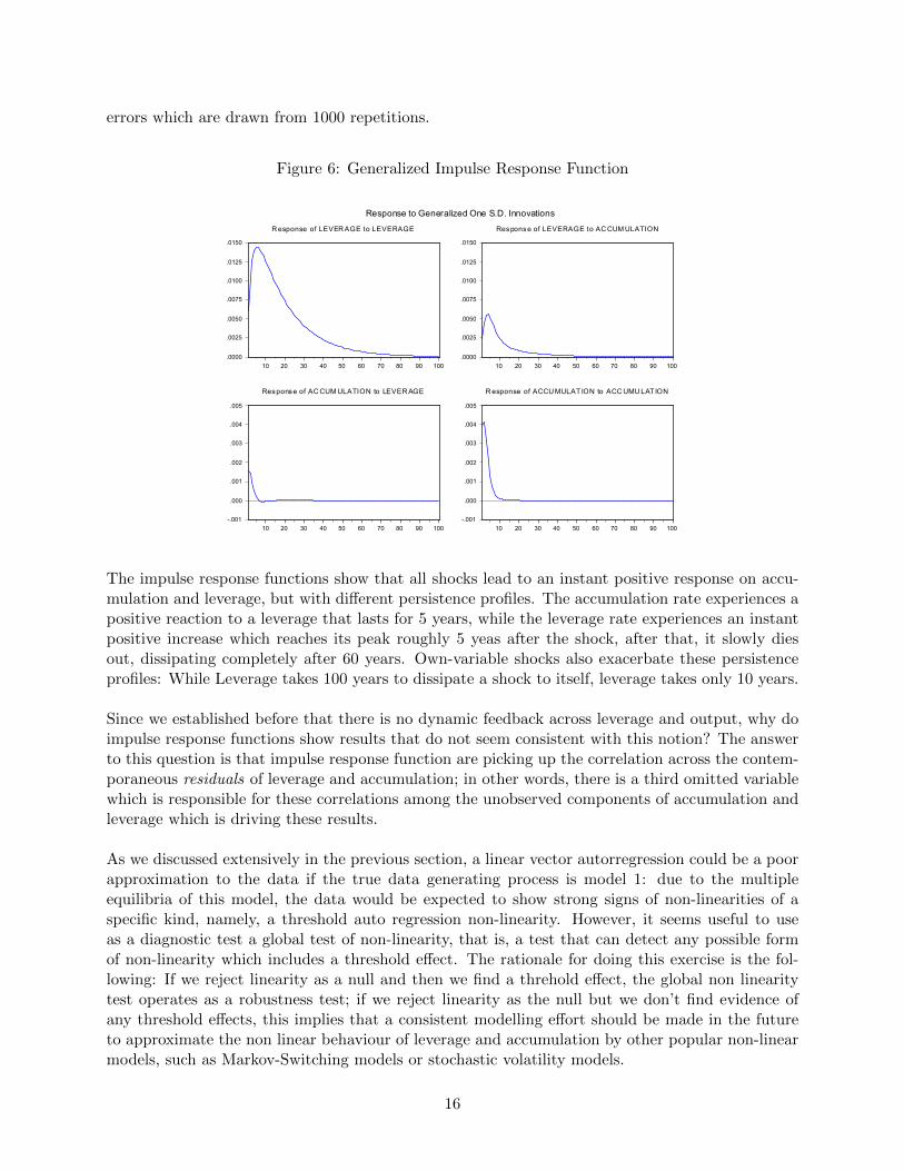
Figure 6: Generalized Impulse Response Function

.0000

.0025

.0050

.0075

.0100

.0125

.0150

10 20 30 40 50 60 70 80 90 100

R esponse of LEVER AGE to LEVERAGE

.0000

.0025

.0050

.0075

.0100

.0125

.0150

10 20 30 40 50 60 70 80 90 100

Response of LEVERAGE to AC CUM ULATION

-.001

.000

.001

.002

.003

.004

.005

10 20 30 40 50 60 70 80 90 100

Response of AC CUM ULATION to LEVER AGE

-.001

.000

.001

.002

.003

.004

.005

10 20 30 40 50 60 70 80 90 100

R esponse of ACCU MULAT ION to ACC UMU LAT ION

Response to Generalized One S.D. Innovations

The impulse response functions show that all shocks lead to an instant positive response on accu-mulation and leverage, but with different persistence profiles. The accumulation rate experiences apositive reaction to a leverage that lasts for 5 years, while the leverage rate experiences an instantpositive increase which reaches its peak roughly 5 yeas after the shock, after that, it slowly diesout, dissipating completely after 60 years. Own-variable shocks also exacerbate these persistenceprofiles: While Leverage takes 100 years to dissipate a shock to itself, leverage takes only 10 years.

Since we established before that there is no dynamic feedback across leverage and output, why doimpulse response functions show results that do not seem consistent with this notion? The answerto this question is that impulse response function are picking up the correlation across the contem-poraneous residuals of leverage and accumulation; in other words, there is a third omitted variablewhich is responsible for these correlations among the unobserved components of accumulation andleverage which is driving these results.

As we discussed extensively in the previous section, a linear vector autorregression could be a poorapproximation to the data if the true data generating process is model 1: due to the multipleequilibria of this model, the data would be expected to show strong signs of non-linearities of aspecific kind, namely, a threshold auto regression non-linearity. However, it seems useful to useas a diagnostic test a global test of non-linearity, that is, a test that can detect any possible formof non-linearity which includes a threshold effect. The rationale for doing this exercise is the fol-lowing: If we reject linearity as a null and then we find a threhold effect, the global non linearitytest operates as a robustness test; if we reject linearity as the null but we don’t find evidence ofany threshold effects, this implies that a consistent modelling effort should be made in the futureto approximate the non linear behaviour of leverage and accumulation by other popular non-linearmodels, such as Markov-Switching models or stochastic volatility models.

16

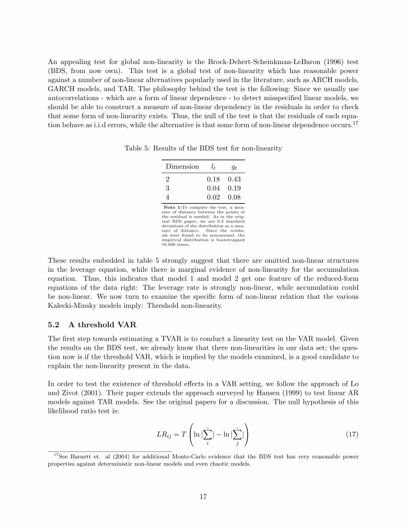
An appealing test for global non-linearity is the Brock-Dehert-Scheinkman-LeBaron (1996) test(BDS, from now own). This test is a global test of non-linearity which has reasonable poweragainst a number of non-linear alternatives popularly used in the literature, such as ARCH models,GARCH models, and TAR. The philosophy behind the test is the following: Since we usually useautocorrelations - which are a form of linear dependence - to detect misspecified linear models, weshould be able to construct a measure of non-linear dependency in the residuals in order to checkthat some form of non-linearity exists. Thus, the null of the test is that the residuals of each equa-tion behave as i.i.d errors, while the alternative is that some form of non-linear dependence occurs.17

Table 5: Results of the BDS test for non-linearity

Dimension lt gt

2 0.18 0.433 0.04 0.194 0.02 0.08

Note 1:To compute the test, a mea-sure of distance between the points ofthe residual is needed. As in the orig-inal BDS paper, we use 0.5 standarddeviations of the distribution as a mea-sure of distance. Since the residu-als were found to be non-normal, theempirical distribution is bootstrapped10.000 times.

These results embedded in table 5 strongly suggest that there are omitted non-linear structuresin the leverage equation, while there is marginal evidence of non-linearity for the accumulationequation. Thus, this indicates that model 1 and model 2 get one feature of the reduced-formequations of the data right: The leverage rate is strongly non-linear, while accumulation couldbe non-linear. We now turn to examine the specific form of non-linear relation that the variousKalecki-Minsky models imply: Threshold non-linearity.

5.2 A threshold VAR

The first step towards estimating a TVAR is to conduct a linearity test on the VAR model. Giventhe results on the BDS test, we already know that there non-linearities in our data set; the ques-tion now is if the threshold VAR, which is implied by the models examined, is a good candidate toexplain the non-linearity present in the data.

In order to test the existence of threshold effects in a VAR setting, we follow the approach of Loand Zivot (2001). Their paper extends the approach surveyed by Hansen (1999) to test linear ARmodels against TAR models. See the original papers for a discussion. The null hypothesis of thislikelihood ratio test is:

LRij = T

ln |∑i

| − ln |∑j

|

(17)

17See Barnett et. al (2004) for additional Monte-Carlo evidence that the BDS test has very reasonable powerproperties against deterministic non-linear models and even chaotic models.

17

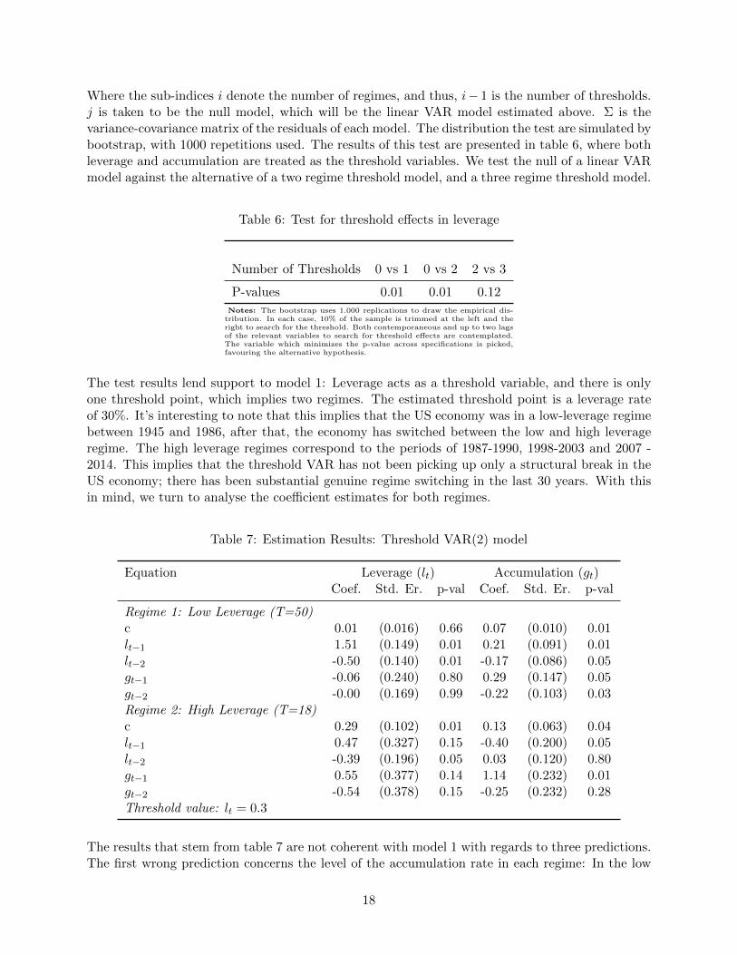
Where the sub-indices i denote the number of regimes, and thus, i− 1 is the number of thresholds.j is taken to be the null model, which will be the linear VAR model estimated above. Σ is thevariance-covariance matrix of the residuals of each model. The distribution the test are simulated bybootstrap, with 1000 repetitions used. The results of this test are presented in table 6, where bothleverage and accumulation are treated as the threshold variables. We test the null of a linear VARmodel against the alternative of a two regime threshold model, and a three regime threshold model.

Table 6: Test for threshold effects in leverage

Number of Thresholds 0 vs 1 0 vs 2 2 vs 3

P-values 0.01 0.01 0.12

Notes: The bootstrap uses 1.000 replications to draw the empirical dis-tribution. In each case, 10% of the sample is trimmed at the left and theright to search for the threshold. Both contemporaneous and up to two lagsof the relevant variables to search for threshold effects are contemplated.The variable which minimizes the p-value across specifications is picked,favouring the alternative hypothesis.

The test results lend support to model 1: Leverage acts as a threshold variable, and there is onlyone threshold point, which implies two regimes. The estimated threshold point is a leverage rateof 30%. It’s interesting to note that this implies that the US economy was in a low-leverage regimebetween 1945 and 1986, after that, the economy has switched between the low and high leverageregime. The high leverage regimes correspond to the periods of 1987-1990, 1998-2003 and 2007 -2014. This implies that the threshold VAR has not been picking up only a structural break in theUS economy; there has been substantial genuine regime switching in the last 30 years. With thisin mind, we turn to analyse the coefficient estimates for both regimes.

Table 7: Estimation Results: Threshold VAR(2) model

Equation Leverage (lt) Accumulation (gt)Coef. Std. Er. p-val Coef. Std. Er. p-val

Regime 1: Low Leverage (T=50)c 0.01 (0.016) 0.66 0.07 (0.010) 0.01lt−1 1.51 (0.149) 0.01 0.21 (0.091) 0.01lt−2 -0.50 (0.140) 0.01 -0.17 (0.086) 0.05gt−1 -0.06 (0.240) 0.80 0.29 (0.147) 0.05gt−2 -0.00 (0.169) 0.99 -0.22 (0.103) 0.03Regime 2: High Leverage (T=18)c 0.29 (0.102) 0.01 0.13 (0.063) 0.04lt−1 0.47 (0.327) 0.15 -0.40 (0.200) 0.05lt−2 -0.39 (0.196) 0.05 0.03 (0.120) 0.80gt−1 0.55 (0.377) 0.14 1.14 (0.232) 0.01gt−2 -0.54 (0.378) 0.15 -0.25 (0.232) 0.28Threshold value: lt = 0.3

The results that stem from table 7 are not coherent with model 1 with regards to three predictions.The first wrong prediction concerns the level of the accumulation rate in each regime: In the low

18

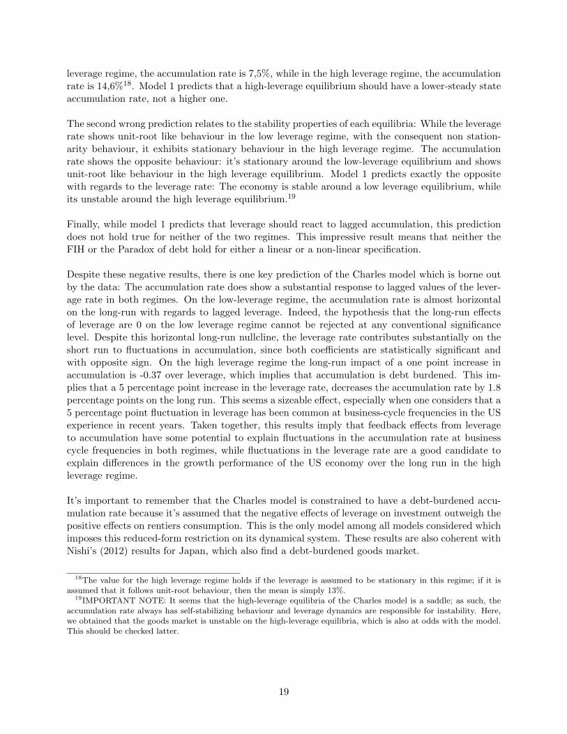
leverage regime, the accumulation rate is 7,5%, while in the high leverage regime, the accumulationrate is 14,6%18. Model 1 predicts that a high-leverage equilibrium should have a lower-steady stateaccumulation rate, not a higher one.

The second wrong prediction relates to the stability properties of each equilibria: While the leveragerate shows unit-root like behaviour in the low leverage regime, with the consequent non station-arity behaviour, it exhibits stationary behaviour in the high leverage regime. The accumulationrate shows the opposite behaviour: it’s stationary around the low-leverage equilibrium and showsunit-root like behaviour in the high leverage equilibrium. Model 1 predicts exactly the oppositewith regards to the leverage rate: The economy is stable around a low leverage equilibrium, whileits unstable around the high leverage equilibrium.19

Finally, while model 1 predicts that leverage should react to lagged accumulation, this predictiondoes not hold true for neither of the two regimes. This impressive result means that neither theFIH or the Paradox of debt hold for either a linear or a non-linear specification.

Despite these negative results, there is one key prediction of the Charles model which is borne outby the data: The accumulation rate does show a substantial response to lagged values of the lever-age rate in both regimes. On the low-leverage regime, the accumulation rate is almost horizontalon the long-run with regards to lagged leverage. Indeed, the hypothesis that the long-run effectsof leverage are 0 on the low leverage regime cannot be rejected at any conventional significancelevel. Despite this horizontal long-run nullcline, the leverage rate contributes substantially on theshort run to fluctuations in accumulation, since both coefficients are statistically significant andwith opposite sign. On the high leverage regime the long-run impact of a one point increase inaccumulation is -0.37 over leverage, which implies that accumulation is debt burdened. This im-plies that a 5 percentage point increase in the leverage rate, decreases the accumulation rate by 1.8percentage points on the long run. This seems a sizeable effect, especially when one considers that a5 percentage point fluctuation in leverage has been common at business-cycle frequencies in the USexperience in recent years. Taken together, this results imply that feedback effects from leverageto accumulation have some potential to explain fluctuations in the accumulation rate at businesscycle frequencies in both regimes, while fluctuations in the leverage rate are a good candidate toexplain differences in the growth performance of the US economy over the long run in the highleverage regime.

It’s important to remember that the Charles model is constrained to have a debt-burdened accu-mulation rate because it’s assumed that the negative effects of leverage on investment outweigh thepositive effects on rentiers consumption. This is the only model among all models considered whichimposes this reduced-form restriction on its dynamical system. These results are also coherent withNishi’s (2012) results for Japan, which also find a debt-burdened goods market.

18The value for the high leverage regime holds if the leverage is assumed to be stationary in this regime; if it isassumed that it follows unit-root behaviour, then the mean is simply 13%.

19IMPORTANT NOTE: It seems that the high-leverage equilibria of the Charles model is a saddle; as such, theaccumulation rate always has self-stabilizing behaviour and leverage dynamics are responsible for instability. Here,we obtained that the goods market is unstable on the high-leverage equilibria, which is also at odds with the model.This should be checked latter.

19

5.3 Are the models consistent with the data?

Given our previous discussion, it seems safe to say that model 3 - the variants proposed by Proffe-sor’s Hein and Lavoie - are not consistent at all with the data. As we’ve seen, a linear specificationimplies essentially no feedback from the relevant endogenous variables, which implies that a linearmodel, such as the one developed by Professor Hein, misses most of the important reduced-formfeatures of the data. The problem with Professor Lavoie’s model is that his low-leverage equilibriumhas a steady-state value of 0 - a prediction also rejected by the data.

Models 2 and 3 can be said to be inconsistent with the data in another very important dimen-sion: Using a one dimension dynamical systems ignores all the relevant feedback from leverage toaccumulation. As we’ve shown, this is the most important empirical fact that arises when we usea non-linear model, since there doesn’t seem to exist any dynamic effects from accumulation toleverage whatsoever. In this sense, future models should seek to explore the dynamic effects ofleverage on aggregate demand, and not only the contemporaneous effects as the literature has doneso far - with the exception of model 1.

One could object to this claims by suggesting that models 2 and 3 predict precisely that accumula-tion has no dynamic effect on leverage; a result which was borne by the data. As such, it could beargued that these models are a reasonable approximation to understand the dynamics of leverageas an univariate process. In Appendix A1 we investigate this claim and provide a negative answer:Whenever we consider leverage in isolation, our data finds 2 thresholds, not 1, as predicted bymodel 2; all the qualitative characteristics of this equilibria are inconsistent with the claims of themodel. As such, even when we give model 2 and 3 a fair chance, they get the non-linear featuresof the data wrong.

Two robustness results which do not essentially change the above discussion are conducted in ap-pendix A1 and A2. In appendix A1, we consider the interest rate of the commercial banking systemexogenous, as it is also assumed in variants of model 2, and include the loan prime rate as an addi-tional regressor. The results on our bivariate or univariate specification do not change at all, sincethe loan prime rate is at best marginally significant in all specifications. In appendix A2, we takeour dependent variable as output growth instead of accumulation. Since the capital to potentialoutput should be fixed in the long run, this implies that these two series should exhibit the samelong-run growth rate. Furthermore, one could argue that Minsky’s reflection about the businesscycle were done in terms of output growth, not in terms the accumulation rate. The results fromthis econometric exercise are disappointing for the Kalecki-Minsky models: In all specifications,there are no feedback effects from output growth to leverage in any sense. Furthermore, leveragedoes not show omitted non-linearities in this specification and output growth acts as the thresholdvariable. Thus, if we take output growth instead of the accumulation rate as the dependent vari-able, all of the predictions by Kalecki-Minsky models are rejected.

In light of the above discussion, we think that the verdict of this empirical investigation is that theCharles model is the only Kaleckian specification which shows some promise of capturing relevantfeatures of the data. More work needs to be done on the feedback channels from lagged leverage tocurrent accumulation, and less work on models which have a solution in terms of a one dimensiondynamical system containing leverage - be it linear o non-linear, since these simple Kalecki-Minskymodels are not relevant to explain the patterns of the data, at least in the US case. However,more empirical work needs to be done taking this family of models to other countries to test their

20

implications before any definite conclusions are reached. Moreover, the implications from Kaldorianand Goodwinian models with Minskian insights also need to be tested, since many variants of thesemodels also imply multiple equilibria and non-linear behaviour.

6 Conclusion

This paper investigates the empirical relevance of Kaleckian model which are augmented by busi-ness debt to produce Minskian insights. In order to do so, it formulates several variants of theKalecki-Minsky models found in the literature, explores what are their main reduced-form impli-cations on the joint dynamics of accumulation and leverage, and shows how linear and non-linearvector autorregressions can be used to test their implications. Specifically, a common feature ofKalecki-Minsky models is their multiple equilibria nature, where one stationary equilibria featuringlow leverage and high accumulation and one non-stationary equilibria featuring high leverage andlow growth are implied by the models. This implies that the Data Generating Process should be athreshold vector auto-regression, which is a specific form of non-linearity.

Using 70 years of US data, this paper finds that the two-equilibria description of accumulation andleverage is borne by the data; furthermore, there exists a threshold effect caused by leverage, notaccumulation, with at most 2 regimes, as predicted by the Charles model. However, many of thequalitative behaviours expected from the Charles model are not borne by the data: One equilibriahas low average leverage and accumulation, while the other has high average leverage and accu-mulation. Furthermore, there is no feedback from accumulation to the leverage rate, contrary towhat is predicted by any of the Kalecki-Minsky variants considered. One key prediction which ischaracteristic of the Charles model is that the accumulation rate is debt-burdened; this implies thatthe negative effects of leverage on investment are higher than their effects on rentiers consumption.It is found that the high-leverage regime is substantially more debt-burdened that the low leverageregime, which implies that the financial behaviour of firm’s have become more important to ex-plaining business cycles and long-run accumulation in the highly leveraged economy that is the US.Overall, while the Charles model can be used as a baseline to understand some relevant features ofthe data, many work still remains to be done to explain the wrong predictions of the Charles model.

Two last comments are in order. First, non-linearity or multiple equilibria are not exclusive fea-tures of the Kalecki-Minsky family, for example, the Goodwin-Minsky model of Keen (1994) is alsoshown to have two equilibria in Grasselli and Costa Lima (2012). The particular feature of Kalecki-Minsky models is that the source of non-linearity is in the behaviour of leverage, while in theGoodwin-Minsky models the Wage Share behaves non-linearly to generate two distinct equilibria.As such, it is certainly promising to study if the labour market feed backs into the accumulationrate in a way that the goods market does not. Second, we ignored Kalecki-Minsky models whichexamine the joint behaviour of accumulation and interest rates (Lima and Meirelles, 2007) or ofthe retention rate and accumulation (Charles, 2008b). Given the results reviewed here, it seemsthat other big families of minskian models or other variants of Kalecki-Minsky models might bepromising avenues of research.

21

Bibliography

Barnett, W. A., Ronald Gallant, A., Hinich, M. J., Jungeilges, J. A., & Kaplan, D. T. (2004). Asingle-blind controlled competition among tests for nonlinearity and chaos. In Functional Structureand Approximation in Econometrics (pp. 581-615). Emerald Group Publishing Limited.

Canova, F. (2007). Methods for applied macroeconomic research (Vol. 13). Princeton UniversityPress.

Charles, S. (2008a). Teaching Minsky’s financial instability hypothesis: a manageable suggestion.Journal of Post Keynesian Economics, 31(1), 125-138.

Charles, S. (2008b). Corporate debt, variable retention rate and the appearance of financial fragility.Cambridge Journal of Economics, 32(5), 781-795.

Charles, S. (2015). Is Minsky’s financial instability hypothesis valid?. Cambridge Journal of Eco-nomics, 40(2), 427-436.

Davis, L. E., De Souza, J. P. A., & Hernandez, G. (2017). An empirical analysis of Minsky regimesin the US economy. UMASS working paper series, 2017-08.

Doornik, J. A., & Hansen, H. (1994). An omnibus test for univariate and multivariate normalit(No. W4&91.). Economics Group, Nuffield College, University of Oxford.

Eggertsson, G. B., & Krugman, P. (2012). Debt, deleveraging, and the liquidity trap: A Fisher-Minsky-Koo approach. The Quarterly Journal of Economics, 127(3), 1469-1513.

Fazzari, S., Ferri, P., & Greenberg, E. (2008). Cash flow, investment, and Keynes-Minsky cycles.Journal of Economic Behavior & Organization, 65(3), 555-572.

Grasselli, M. R., & Lima, B. C. (2012). An analysis of the Keen model for credit expansion, assetprice bubbles and financial fragility. Mathematics and Financial Economics, 6(3), 191.

Hansen, B. E. (2011). Threshold autoregression in economics. Statistics and its Interface, 4(2),123-127.

Hamilton, J. D. (2008). Macroeconomics and ARCH (No. w14151). National Bureau of EconomicResearch.

Hein, E. (2007). Interest rate, debt, distribution and capital accumulation in a post-Kaleckianmodel. Metroeconomica, 58(2), 310-339.

Hein, E. (2014). Distribution and growth after Keynes: A Post-Keynesian guide. Edward ElgarPublishing.

Juselius, K. (2006). The cointegrated VAR model: methodology and applications. Oxford univer-sity press.

22

Kalecki, M. (1937). The principle of increasing risk. Economica, 4(16), 440-447.

King, R. G., & Rebelo, S. T. (1999). Resuscitating real business cycles. Handbook of macroeco-nomics, 1, 927-1007.

Hubrich, K., & Terasvirta, T. (2013). Thresholds and Smooth Transitions in Vector Autoregres-sive Models. In ’VAR Models in Macroeconomics–New Developments and Applications: Essays inHonor of Christopher A. Sims (pp. 273-326)’. Emerald Group Publishing Limited.

Lavoie, M. (1995). Interest Rates in Post-Keynesian Models of Growth and Distribution. Metroe-conomica, 46(2), 146-177.

Lavoie, M. (2009). Towards a post-Keynesian consensus in macroeconomics: Reconciling the Cam-bridge and Wall Street views. Macroeconomic Policies on Shaky Foundations–Whither MainstreamEconomics, 75-99.

Lavoie, M. (2014). Post-Keynesian economics: new foundations. Edward Elgar Publishing.

Lima, G. T., & Meirelles, A. J. (2007). Macrodynamics of debt regimes, financial instability andgrowth. Cambridge Journal of Economics, 31(4), 563-580.

Nishi, H. (2012). Structural VAR analysis of debt, capital accumulation, and income distributionin the Japanese economy: a Post Keynesian perspective. Journal of Post Keynesian Economics,34(4), 685-712.

Nikolaidi, M., & Stockhammer, E. (2017). Minsky models. A structured survey.

Minsky, H. (1975). John Maynard Keynes. Columbia University Press: New York.

Minsky, H. (1982) Can “It” Happen Again. Essays on Stability and Finance. M.E. Sharpe: NewYork.

Minsky, H. (1986) Stabilizing an Unstable Economy. Yale University Press: New Haven

Minsky, H. (1992) The Financial Instability Hypothesis. Levy Economics Institute. Working PaperNo.74.

Ryoo, S. (2013a). The paradox of debt and Minsky’s financial instability hypothesis. Metroeco-nomica, 64(1), 1-24.

Ryoo, S. (2013b). Bank profitability, leverage and financial instability: a Minsky–Harrod model.Cambridge journal of economics, 37(5), 1127-1160.

Hirsch, M. W., Smale, S., & Devaney, R. L. (2012). Differential equations, dynamical systems, andan introduction to chaos. Academic press.

Skott, P. (2013). Increasing inequality and financial instability. Review of Radical Political Eco-nomics, 45(4), 478-488.

23

Stockhammer, E. (2005). Shareholder value orientation and the investment-profit puzzle. Journalof Post Keynesian Economics, 28(2), 193-215.

Stock, J. H., & Watson, M. W. (1999). Business cycle fluctuations in US macroeconomic timeseries. Handbook of macroeconomics, 1, 3-64.

24