Are GANs Created Equal? A Large-Scale Study · PDF fileAre GANs Created Equal? A Large-Scale...

Are GANs Created Equal? A Large-Scale Study

Mario Lucic? Karol Kurach? Marcin Michalski Sylvain Gelly Olivier BousquetGoogle Brain

Abstract

Generative adversarial networks (GAN) are a powerfulsubclass of generative models. Despite a very rich researchactivity leading to numerous interesting GAN algorithms, itis still very hard to assess which algorithm(s) perform bet-ter than others. We conduct a neutral, multi-faceted large-scale empirical study on state-of-the art models and evalu-ation measures. We find that most models can reach similarscores with enough hyperparameter optimization and ran-dom restarts. This suggests that improvements can arisefrom a higher computational budget and tuning more thanfundamental algorithmic changes. To overcome some limi-tations of the current metrics, we also propose several datasets on which precision and recall can be computed. Our ex-perimental results suggest that future GAN research shouldbe based on more systematic and objective evaluation pro-cedures. Finally, we did not find evidence that any of thetested algorithms consistently outperforms the original one.

1. IntroductionGenerative adversarial networks (GAN) are a power-

ful subclass of generative models and were successfullyapplied to image generation and editing, semi-supervisedlearning, and domain adaptation [20, 24]. In the GANframework the model learns a deterministic transformationG of a simple distribution pz , with the goal of matching thedata distribution pd. This learning problem may be viewedas a two-player game between the generator, which learnshow to generate samples which resemble real data, and adiscriminator, which learns how to discriminate betweenreal and fake data. Both players aim to minimize their owncost and the solution to the game is the Nash equilibriumwhere neither player can improve their cost unilaterally [8].

Various flavors of GANs have been recently proposed,both purely unsupervised [8, 1, 9, 4] as well as conditional[18, 19]. While these models achieve compelling results inspecific domains, there is still no clear consensus on whichGAN algorithm(s) perform objectively better than others.

?Indicates equal authorship. Correspondence to Mario Lucic ([email protected]) and Karol Kurach ([email protected]).

This is partially due to the lack of robust and consistentmetric, as well as limited comparisons which put all algo-rithms on equal footage, including the computational bud-get to search over all hyperparameters. Why is it impor-tant? Firstly, to help the practitioner choose a better algo-rithm from a very large set. Secondly, to make progress to-wards better algorithms and their understanding, it is usefulto clearly assess which modifications are critical, and whichones are only good on paper, but do not make a significantdifference in practice.

The main issue with evaluation stems from the fact thatone cannot explicitly compute the probability pg(x). As aresult, classic measures, such as log-likelihood on the testset, cannot be evaluated. Consequently, many researchersfocused on qualitative comparison, such as comparing thevisual quality of samples. Unfortunately, such approachesare subjective and possibly misleading [7].

As a remedy, two evaluation metrics were proposed toquantitatively assess the performance of GANs. Both as-sume access to a pre-trained classifier. Inception Score (IS)[21] is based on the fact that a good model should gen-erate samples for which, when evaluated by the classifier,the class distribution has low entropy. At the same time,it should produce diverse samples covering all classes. Incontrast, Frechet Inception Distance is computed by con-sidering the difference in embedding of true and fake data[10]. Assuming that the coding layer follows a multivariateGaussian distribution, the distance between the distributionsis reduced to the Frechet distance between the correspond-ing Gaussians.

Our main contributions:1. We provide a fair and comprehensive comparison of

the state-of-the-art GANs, and empirically demon-strate that nearly all of them can reach similar valuesof FID, given a high enough computational budget.

2. We provide strong empirical evidence1 that to compareGANs it is necessary to report a summary of distri-bution of results, rather than the best result achieved,due to the randomness of the optimization process andmodel instability.

1As a note on the scale of the setup, the computational budget to repro-duce those experiments is approximately 6.85 GPU years (NVIDIA P100).

1

arX

iv:1

711.

1033

7v3

[st

at.M

L]

20

Mar

201

8

3. We assess the robustness of FID to mode dropping, useof a different encoding network, and provide estimatesof the best FID achievable on classic data sets.

4. We introduce a series of tasks of increasing difficultyfor which undisputed measures, such as precision andrecall, can be approximately computed.

5. We open-sourced our experimental setup and modelimplementations at goo.gl/G8kf5J.

2. Background and Related WorkThere are several ongoing challenges in the study of

GANs, including their convergence properties [2, 17], andoptimization stability [21, 1]. Arguably, the most criticalchallenge is their quantitative evaluation.

The classic approach towards evaluating generative mod-els is based on model likelihood which is often intractable.While the log-likelihood can be approximated for distribu-tions on low-dimensional vectors, in the context of complexhigh-dimensional data the task becomes extremely chal-lenging. Wu et al. [23] suggest an annealed importancesampling algorithm to estimate the hold-out log-likelihood.The key drawback of the proposed approach is the assump-tion of the Gaussian observation model which carries overall issues of kernel density estimation in high-dimensionalspaces. Theis et al. [22] provide an analysis of commonfailure modes and demonstrate that it is possible to achievehigh likelihood, but low visual quality, and vice-versa. Fur-thermore, they argue against using Parzen window densityestimates as the likelihood estimate is often incorrect. In ad-dition, ranking models based on these estimates is discour-aged [3]. For a discussion on other drawbacks of likelihood-based training and evaluation consult Huszar [11].

Inception Score (IS). Proposed by [21], IS offers a wayto quantitatively evaluate the quality of generated samples.The score was motivated by the following considerations:(i) The conditional label distribution of samples containingmeaningful objects should have low entropy, and (ii) Thevariability of the samples should be high, or equivalently,the marginal

∫zp(y|x = G(z))dz should have high entropy.

Finally, these desiderata are combined into one score,

IS(G) = exp(Ex∼G[dKL(p(y | x), p(y)])

The classifier is Inception Net trained on Image Netwhich is publicly available. The authors found that thisscore is well-correlated with scores from human annotators[21]. Drawbacks include insensitivity to the prior distribu-tion over labels and not being a proper distance.

Frechet Inception Distance (FID). Proposed by [10],FID provides an alternative approach. To quantify the qual-ity of generated samples, they are first embedded into afeature space given by (a specific layer) of Inception Net.Then, viewing the embedding layer as a continuous multi-variate Gaussian, the mean and covariance is estimated for

both the generated data and the real data. The Frechet dis-tance between these two Gaussians is then used to quantifythe quality of the samples, i.e.

FID(x, g) = ||µx − µg||22 + Tr(Σx + Σg − 2(ΣxΣg)12 ),

where (µx,Σx), and (µg,Σg) are the mean and covarianceof the sample embeddings from the data distribution andmodel distribution, respectfully. The authors show that thescore is consistent with human judgment and more robust tonoise than IS [10]. Furthermore, the authors present com-pelling results showing negative correlation between theFID and visual quality of generated samples. Unlike IS,FID can detect intra-class mode dropping, i.e. a model thatgenerates only one image per class can score a perfect IS,but will have a bad FID. We provide a thorough empiricalanalysis of FID in Section 5.

A significant drawback of both measures is the inabilityto detect overfitting. A “memory GAN” which stores alltraining samples would score perfectly.

A very recent study comparing several GANs using IShas been presented by Fedus et al. [6]. The authors focuson IS and consider a smaller subset of GANs. In contrast,our focus is on providing a fair assessment of the currentstate-of-the-art GANs using FID, as well as precision andrecall, and also verifying the robustness of these models ina large-scale empirical evaluation.

3. Flavors of Generative Adversarial NetworksIn this work we focus on unconditional generative ad-

versarial networks. In this setting, only unlabeled data isavailable for learning. The optimization problems arisingfrom existing approaches differ by (i) the constraint on thediscriminators output and corresponding loss, and the pres-ence and application of gradient norm penalty.

In the original GAN formulation [8] two loss functionswere proposed. In the minimax GAN the discriminator out-puts a probability and the loss function is the negative log-likelihood of a binary classification task (MM GAN in Ta-ble 1). Here the generator learns to generate samples thathave a low probability of being fake. To improve the gradi-ent signal, the authors also propose the non-saturating loss(NS GAN in Table 1), where the generator instead aims tomaximize the probability of generated samples being real.

In Wasserstein GAN [1] the discriminator is allowed tooutput a real number and the objective function is equiva-lent to the MM GAN loss without the sigmoid (WGAN inTable 1). The authors prove that, under an optimal (Lips-chitz smooth) discriminator, minimizing the value functionwith respect to the generator minimizes the Wasserstein dis-tance between model and data distributions. Weights of thediscriminator are clipped to a small absolute value to en-force smoothness. To improve on the stability of the train-ing, Gulrajani et al. [9] instead add a soft constraint on the

Table 1: Generator and discriminator loss functions. The main difference whether the discriminator outputs a probability (MM GAN, NS

GAN, DRAGAN) or its output is unbounded (WGAN, WGAN GP, LS GAN, BEGAN), whether the gradient penalty is present (WGAN GP,DRAGAN) and where is it evaluated. We chose those models based on their popularity.

GAN DISCRIMINATOR LOSS GENERATOR LOSS

MM GAN LGAND = −Ex∼pd [log(D(x))]− Ex∼pg [log(1−D(x))] LGAN

G = Ex∼pg [log(1−D(x))]

NS GAN LNSGAND = −Ex∼pd [log(D(x))]− Ex∼pg [log(1−D(x))] LNSGAN

G = −Ex∼pg [log(D(x))]

WGAN LWGAND = −Ex∼pd [D(x)] + Ex∼pg [D(x)] LWGAN

G = −Ex∼pg [D(x)]

WGAN GP LWGANGPD = LWGAN

D + λEx∼pg [(||∇D(αx+ (1− αx)||2 − 1)2] LWGANGPG = −Ex∼pg [D(x)]

LS GAN LLSGAND = −Ex∼pd [(D(x)− 1)2] + Ex∼pg [D(x)2] LLSGAN

G = −Ex∼pg [(D(x− 1)2]

DRAGAN LDRAGAND = LGAN

D + λEx∼pd+N (0,c)[(||∇D(x)||2 − 1)2] LDRAGANG = Ex∼pg [log(1−D(x))]

BEGAN LBEGAND = Ex∼pd [||x− AE(x)||1]− ktEx∼pg [||x− AE(x)||1] LBEGAN

G = Ex∼pg [||x− AE(x)||1]

norm of the gradient which encourages the discriminator tobe 1-Lipschitz. The gradient norm is evaluated on pointsobtained by linear interpolation between data points andgenerated samples where the optimal discriminator shouldhave unit gradient norm [9].

Gradient norm penalty can also be added to both MMGAN and NS GAN and evaluated around the data manifold(DRAGAN [14] in Table 1 based on NS GAN). This encour-ages the discriminator to be piecewise linear around the datamanifold. Note that the gradient norm can also be evaluatedbetween fake and real points, similarly to WGAN GP, andadded to either MM GAN or NS GAN [6].

Mao et al. [16] propose a least-squares loss for the dis-criminator and show that minimizing the corresponding ob-jective (LS GAN in Table 1) implicitly minimizes the Pear-son χ2 divergence. The idea is to provide smooth loss whichsaturates slower than the sigmoid cross-entropy loss of theoriginal MM GAN.

Finally, Berthelot et al. [4] propose to use an autoen-coder as a discriminator and optimize a lower bound of theWasserstein distance between auto-encoder loss distribu-tions on real and fake data. They introduce an additionalhyperparameter γ to control the equilibrium between thegenerator and discriminator.

4. Challenges of a Fair Comparison

There are several interesting dimensions to this problem,and there is no single right way to compare these models(i.e. the loss function used in each GAN). Unfortunately,due to the combinatorial explosion in the number of choicesand their ordering, not all relevant options can be explored.While there is no definite answer on how to best comparetwo models, in this work we have made several pragmatic

choices which were motivated by two practical concerns:providing a neutral and fair comparison, and a hard limit onthe computational budget.

Which metric to use? Comparing models implies ac-cess to some metric. As discussed in Section 2, classic mea-sures, such as model likelihood cannot be applied. We willargue for and study two sets of evaluation metrics in Sec-tion 5: FID, which can be computed on all data sets, andprecision, recall, and F1, which we can compute for theproposed tasks.

How to compare models? Even when the metric isfixed, a given algorithm can achieve very different scores,when varying the architecture, hyperparameters, randominitialization (i.e. random seed for initial network weights),or the data set. Sensible targets include best score acrossall dimensions (e.g. to claim the best performance on afixed data set), average or median score (rewarding modelswhich are good in expectation), or even the worst score (re-warding models with worst-case robustness). These choicescan even be combined — for example, one might train themodel multiple times using the best hyperparameters, andaverage the score over random initializations).

For each of these dimensions, we took several pragmaticchoices to reduce the number of possible configurations,while still exploring the most relevant options.

1. Architecture: We use the same architecture for allmodels. The architecture is rich enough to achievegood performance.

2. Hyperparameters: For both training hyperparameters(e.g. the learning rate), as well as model specific ones(e.g. gradient penalty multiplier), there are two validapproaches: (i) perform the hyperparameter optimiza-tion for each data set, or (ii) perform the hyperparame-

ter optimization on one data set and infer a good rangeof hyperparameters to use on other data sets. We ex-plore both avenues in Section 6.

3. Random seed: Even with everything else being fixed,varying the random seed may have a non-trivial influ-ence on the results. We study this particular effect andreport the corresponding confidence intervals.

4. Data set: We chose four popular data sets from GANliterature and report results separately for each data set.

5. Computational budget: Depending on the budgetto optimize the parameters, different algorithms canachieve the best results. We explore how the resultsvary depending on the budget.

In practice, one can either use hyperparameter valuessuggested by respective authors, or try to optimize them.Figure 5 and in particular Figure 15 show that optimizationis necessary. Hence, we optimize the hyperparameters foreach model and data set by performing a random search.2

We concur that the models with fewer hyperparameters havean advantage over models with many hyperparameters, butconsider this fair as it reflects the experience of practitionerssearching for good hyperparameters for their setting.

5. Metrics

In this work we focus on two sets of metrics. We first an-alyze the recently proposed FID in terms of robustness (ofthe metric itself), and conclude that it has desirable proper-ties and can be used in practice. Nevertheless, this metric,as well as Inception Score, is incapable of detecting overfit-ting: a memory GAN which simply stores all training sam-ples would score perfectly under both measures. Based onthese shortcomings, we propose an approximation to pre-cision and recall for GANs and how that it can be used toquantify the degree of overfitting. We stress that the pro-posed method should be viewed as complementary to IS orFID, rather than a replacement.

5.1. Frechet Inception Distance

FID was shown to be robust to noise [10]. Here we quan-tify the bias and variance of FID, its sensitivity to the encod-ing network and sensitivity to mode dropping. To this end,we partition the data set into two groups, i.e. X = X1 ∪X2.Then, we define the data distribution pd as the empiricaldistribution on a random subsample of X1 and the modeldistribution pg to be the empirical distribution on a randomsubsample fromX2. For a random partition this “model dis-tribution” should follow the data distribution.

Bias and variance. We evaluate the bias and variance ofFID on four classic data sets used in the GAN literature. We

2Furthermore, while we present the results which were obtained by arandom search, we have also investigated sequential Bayesian optimiza-tion, which resulted in comparable results.

Table 2: Bias and variance of FID. If the data distribution matchesthe model distribution, FID should evaluate to zero. However, weobserve some bias and low variance on samples of size 10000.

DATA SET AVG. FID DEV. FID

CELEBA 2.27 0.02CIFAR10 5.19 0.02FASHION-MNIST 2.60 0.03MNIST 1.25 0.02

start by using the default train vs. test partition and computethe FID between the test set (limited to N = 10000 sam-ples for CelebA) and the sample of size N from the trainset. The sampling from the train set is performed M = 50times. The optimistic estimate of FID are reported in Ta-ble 2. We observe that FID has rather high bias, but smallvariance. From this perspective, estimating the full covari-ance matrix might be unnecessary and counter-productive,and a constrained version might suffice.

To test the sensitivity to this initial choice of train vs. testpartitioning, we consider 50 random partitions (keeping therelative sizes fixed, i.e. 6 : 1 for MNIST) and compute theFID with M = 1 sample. We observe results similar toTable 2 which is to be expected if the train and test data setsare drawn from the same distribution.

Detecting mode dropping with FID. To simulate miss-ing modes, we fix a partition of data set X = X1 ∪ X2 andwe subsample X2 and keep only samples from the first kclasses, increasing k from 1 to 10. For each k, we consider50 random subsamples from X2. Figure 1 shows that FID isheavily influenced by the missing modes.

1 2 3 4 5 6 7 8 9 10

Number of classes

0

20

40

60

80

Frech

et

Ince

pti

on D

ista

nce

Data set

CIFAR10

FASHION-MNIST

MNIST

Figure 1: As the sample captures more classes the FID with re-spect to the reference data set decreases. We observe that FIDdrastically increases under mode dropping.

Sensitivity to encoding network. Suppose we computeFID using a different network and encoding layer. Wouldthe ranking of models change? To test this we apply VGGtrained on ImageNet and consider the layer FC7 of dimen-sion 4096. Figure 2 shows the resulting distribution. Weobserve high Spearman’s rank correlation ρ = 0.9 whichencourages the use of the default coding layer suggested by

0 50 100 150 200 250FID (Inception)

0

5

10

15

20

25

30

35

FID

(V

GG

) (I

n t

housa

nds)

pearsonr = 0.9; p = 0

Figure 2: The difference between FID score computed on Incep-tionNet vs FID computed using VGG for the CELEBA data set (forinteresting range: FID < 200). We observe high rank correlation(Spearman’s ρ = 0.9) which encourages the use of the defaultcoding layer suggested by the authors.

the authors. Of course, a natural comparison would be toapply VGG trained on some other data set, which we leavefor future work.

5.2. Precision, Recall and F1 Score

Precision, recall and F1 score are proven and widelyadopted techniques for quantitatively evaluating the qualityof discriminative models. Precision measures the fraction ofrelevant retrieved instances among the retrieved instances,while recall measures the fraction of the retrieved instancesamong relevant instances. F1 score is the harmonic averageof precision and recall.

Notice that IS only captures precision: It will not penal-ize the model for not producing all modes of the data distri-bution — it will only penalize the model for not producingall classes. On the other hand, FID captures both precisionand recall. Indeed, a model which fails to recover differentmodes of the data distribution will suffer in terms of FID.

We propose a simple and effective data set for evaluating(and comparing) generative models. Our main motivationis that the currently used data sets are either too simple (e.g.simple mixtures of Gaussians, or MNIST) or too complex(e.g. ImageNet). We argue that it is critical to be able toincrease the complexity of the task in a relatively smoothand controlled fashion. To this end, we present a set of tasksfor which we can approximate the precision and recall ofeach model. As a result, we can compare different modelsbased on established metrics.

Manifold of convex polygons. The main idea is to con-struct a data manifold such that the distances from samplesto the manifold can be computed efficiently. As a result, theproblem of evaluating the quality of the generative modelis effectively transformed into a problem of computing the

(a) High precision, high recall (b) High precision, low recall

(c) Low precision, high recall (d) Low precision, low recall

Figure 3: Samples from models with (a) high recall and precision,(b) high precision, but low recall (lacking in diversity), (c) lowprecision, but high recall (can decently reproduce triangles, butfails to capture convexity), and (d) low precision and low recall.

distance to the manifold. This enables an intuitive approachfor defining the quality of the model. Namely, if the sam-ples from the model distribution pg are (on average) closeto the manifold, its precision is high. Similarly, high recallimplies that the generator can recover (i.e. generate some-thing close to) any sample from the manifold.

For general data sets, this reduction is impractical as onehas to compute the distance to the manifold which we aretrying to learn. However, if we construct a manifold suchthat this distance is efficiently computable, the precision andrecall can be efficiently evaluated.

To this end, we propose a set of toy data sets for whichsuch computation can be performed efficiently: The mani-fold of convex polygons. As the simplest example, let usfocus on gray-scale triangles represented as one channelimages as in Figure 3. These triangles belong to a low-dimensional manifold C3 embedded in Rd×d. Intuitively,the coordinate system of this manifold represents the axesof variation (e.g. rotation, translation, minimum angle size,etc.). A good generative model should be able to capturethese factors of variation and recover the training samples.Furthermore, it should recover any sample from this man-ifold from which we can efficiently sample which is illus-trated in Figure 3.

Computing the distance to the manifold. Let us con-sider the simplest case: single-channel gray scale imagesrepresented as vectors x ∈ Rd2

. The distance of a sample

5 10 15 20 25 30 35 40 45 50 55 60 65 70

Budget

0

5

10

15

20

25

30

35

40

FID

Data set = MNIST

5 10 15 20 25 30 35 40 45 50 55 60 65 70

Budget

10

20

30

40

50

60

70

80

90

100Data set = FASHION-MNIST

5 10 15 20 25 30 35 40 45 50 55 60 65 70

Budget

60

80

100

120

140

Data set = CIFAR10

5 10 15 20 25 30 35 40 45 50 55 60 65 70

Budget

40

60

80

100

120

Data set = CELEBA

Model

BEGAN

DRAGAN

LSGAN

MM GAN

NS GAN

WGAN

WGAN GP

Figure 4: How does the minimum FID behave as a function of the budget? The plot shows the distribution of the minimum FID achievablefor a fixed budget along with one standard deviation interval. For each budget, we estimate the mean and variance using 5000 bootstrapresamples out of 100 runs. We observe that, given a relatively low budget (say less than 15 hyperparameter settings), all models achievea similar minimum FID. Furthermore, for a fixed FID, “bad” models can outperform “good” models given enough computational budget.We argue that the computational budget to search over hyperparameters is an important aspect of the comparison between algorithms.

x ∈ Rd2

to the manifold is defined as the squared Euclideandistance to the closest sample from the manifold C3, i.e.

minx∈C3

`(x, x) =d2∑

i=1

||xi − xi||22.

This is a non-convex optimization problem. We find an ap-proximate solution by gradient descent on the vertices ofthe triangle (more generally, a convex polygon), ensuringthat each iterate is a valid triangle (more generally, a con-vex polygon). To reduce the false-negative rate we repeatthe algorithm several times from random initial solutions.

To compute the latent representation of a sample x ∈Rd×d we invert the generator, i.e. we solve

z? = arg minz∈Rdz ||x−G(z)||22,using gradient descent on z while keeping G fixed [15].

6. Large-scale Experimental EvaluationWe consider two budget-constrained experimental setups

whereby in the (i) wide one-shot setup one may select100 samples of hyper-parameters per model, and where therange for each hyperparameter is wide, and (ii) the narrowtwo-shots setup where one is allowed to select 50 samplesfrom more narrow ranges which were manually selectedby first performing the wide hyperparameter search over aspecific data set. For the exact ranges and hyperparametersearch details we refer the reader to the Appendix A. In thesecond set of experiments we evaluate the models based onthe ”novel” metric: F1 score on the proposed data set. Fi-nally, we included the Variational Autoencoder [13] in theexperiments as a popular alternative.

6.1. Experimental Setup

To ensure a fair comparison, we made the followingchoices: (i) we use the generator and discriminator archi-tecture from INFO GAN [5] as the resulting function space

is rich enough and all considered GANs were not originallydesigned for this architecture. Furthermore, it is similar toa proven architecture used in DCGAN [20]. The exceptionis BEGAN where an autoencoder is used as the discrimina-tor. We maintain similar expressive power to INFO GANby using identical convolutional layers the encoder and ap-proximately matching the total number of parameters.

For all experiments we fix the latent code size to 64 andthe prior distribution over the latent space to be uniform on[−1, 1]64, except for VAE where it is Gaussian N (0, I). Wechoose Adam [12] as the optimization algorithm as it wasthe most popular choice in the GAN literature 3. We applythe same learning rate for both generator and discriminator.We set the batch size to 64 and perform optimization for 20epochs on MNIST and FASHION MNIST, 40 on CELEBA and100 on CIFAR4.

Finally, we allow for recent suggestions, such as batchnormalization in the discriminator, and imbalanced updatefrequencies of generator and discriminator. We explorethese possibilities, together with learning rate, parameter β1for ADAM, and hyperparameters of each model. We reportthe hyperparameter ranges and other details in Appendix A.

6.2. A Large Hyperparameter Search

We perform hyperparameter optimization and, for eachrun, look for the best FID across the training run (simulatingearly stopping). To choose the best model, every 5 epochswe compute the FID between the 10k samples generated bythe model and the 10k samples from the test set. We haveperformed this computationally expensive search for eachdata set. We present the sensitivity of models to the hyper-parameters in Figure 5 and the best FID achieved by eachmodel in Table 3.

3An empirical comparison to RMSProp is provided in Appendix F4Those four data sets are a popular choice for generative modeling.

They are of simple to medium complexity, making it possible to run manyexperiments as well as getting decent results.

MM G

AN

NS GAN

LSGAN

WGAN

WGAN G

P

DRAGAN

BEGAN

VAE

Model

10

20

30

40

50

60

FID

Sco

re

Dataset = MNIST

MM G

AN

NS GAN

LSGAN

WGAN

WGAN G

P

DRAGAN

BEGAN

VAE

Model

20

40

60

80

100

120

140

Dataset = FASHION-MNIST

MM G

AN

NS GAN

LSGAN

WGAN

WGAN G

P

DRAGAN

BEGAN

VAE

Model

50

100

150

200

250Dataset = CIFAR10

MM G

AN

NS GAN

LSGAN

WGAN

WGAN G

P

DRAGAN

BEGAN

VAE

Model

50

100

150

200

250Dataset = CELEBA

Figure 5: A wide range hyperparameter search (100 hyperparameter samples per model). Black stars indicate the performance of sug-gested hyperparameter settings. We observe that GAN training is extremely sensitive to hyperparameter settings and there is no modelwhich is significantly more stable than others. The importance of hyperparameter search is further highlighted in Figure 15.

Table 3: Best FID obtained in a large-scale hyperparametersearch for each data set. The scores were computed in twophases: first, we run a large-scale search on a wide range of hyper-parameters, and select the best model. Then, we re-run the trainingof the selected model 50 times with different initialization seeds, toestimate the stability of the training and report the mean FID andstandard deviation, excluding outliers. The asterisk (*) on somecombinations of models and data sets indicates the presence ofsignificant outlier runs, usually severe mode collapses or trainingfailures (** indicates up to 20% failures). We observe that the per-formance of each model heavily depends on the data set and nomodel strictly dominates the others. We note that VAE is heav-ily penalized due to the blurriness of the generated images. Notethat these results are not “state-of-the-art”: (i) larger architec-tures could improve all models, (ii) authors often report the bestFID which opens the door for random seed optimization.

MNIST FASHION CIFAR CELEBA

MM GAN 9.8± 0.9 29.6± 1.6 72.7± 3.6 65.6± 4.2NS GAN 6.8± 0.5 26.5± 1.6 58.5± 1.9 55.0± 3.3LSGAN 7.8± 0.6* 30.7± 2.2 87.1± 47.5 53.9± 2.8*WGAN 6.7± 0.4 21.5± 1.6 55.2± 2.3 41.3± 2.0WGAN GP 20.3± 5.0 24.5± 2.1 55.8± 0.9 30.0± 1.0DRAGAN 7.6± 0.4 27.7± 1.2 69.8± 2.0 42.3± 3.0BEGAN 13.1± 1.0 22.9± 0.9 71.4± 1.6 38.9± 0.9VAE 23.8± 0.6 58.7± 1.2 155.7± 11.6 85.7± 3.8

Critically, we consider the mean FID as the computa-tional budget increases which is shown in Figure 4. Thereare three important observations. Firstly, there is no algo-rithm which clearly dominates others. Secondly, for an in-teresting range of FIDs, a “bad” model trained on a largebudget can out perform a “good” model trained on a smallbudget. Finally, when the budget is limited, any statisticallysignificant comparison of the models is unattainable.

6.3. Impact of Limited Computational Budget

In some cases, the computational budget available to apractitioner is too small to perform such a large-scale hy-perparameter search. Instead, one can tune the range of hy-perparameters on one data set and interpolate the good hy-

perparameter ranges for other data sets. We now considerthis setting in which we allow only 50 samples from a set ofnarrow ranges, which were selected based on the wide hy-perparameter search on the FASHION-MNIST data set. Wereport the narrow hyperparameter ranges in Appendix A.

Figure 15 shows the variance of FID per model, wherethe hyperparameters were selected from narrow ranges.From the practical point of view, there are significant dif-ferences between the models: in some cases the hyperpa-rameter ranges transfer from one data set to the others (e.g.NS GAN), while others are more sensitive to this choice(e.g. WGAN). We note that better scores can be obtainedby a wider hyperparameter search. These results supportsthe conclusion that discussing the best score obtained bya model on a data set is not a meaningful way to discernbetween these models. One should instead discuss the dis-tribution of the obtained scores.

6.4. Robustness to Random Initialization

For a fixed model, hyperparameters, training algorithm,and the order that the data is presented to the model, onewould expect similar model performance. To test this hy-pothesis we re-train the best models from the limited hyper-parameter range considered for the previous section, whilechanging the initial weights of the generator and discrimi-nator networks (i.e. by varying a random seed). Table 3 andFigure 16 show the results for each data set. Most modelsare relatively robust to random initialization, except LSGAN,even though for all of them the variance is significant andshould be taken into account when comparing models.

6.5. Precision, recall, and F1

We perform a search over the wide range of hyperpa-rameters and compute precision and recall by consideringn = 1024 samples. In particular, we compute the precisionof the model by computing the fraction of generated sam-ples with distance below a threshold δ = 0.75. We thenconsider n samples from the test set and invert each sample

5 10 15 20 25 30 35 40 45 50 55 60 65 70

Budget

0.2

0.0

0.2

0.4

0.6

0.8

1.0

Valu

e

Measure = F1

5 10 15 20 25 30 35 40 45 50 55 60 65 70

Budget

0.3

0.4

0.5

0.6

0.7

0.8

0.9

1.0

1.1Measure = Precision

5 10 15 20 25 30 35 40 45 50 55 60 65 70

Budget

0.0

0.2

0.4

0.6

0.8

Measure = Recall

Model

BEGAN

DRAGAN

MM GAN

NS GAN

WGAN

WGAN GP

Figure 6: How does F1 score vary with computational budget? The plot shows the distribution of the maximum F1 score achievablefor a fixed budget with a 95% confidence interval. For each budget, we estimate the mean and confidence interval (of the mean) using5000 bootstrap resamples out of 100 runs. When optimizing for F1 score, both NS GAN and WGAN enjoy high precision and recall. Theunderwhelming performance of BEGAN and VAE on this particular data set merits further investigation.

x to compute z? = G−1(x) and compute the squared Eu-clidean distance between x and G(z?). We define the recallas the fraction of samples with squared Euclidean distancebelow δ. Figure 6 shows the results where we select the bestF1 score for a fixed model and hyperparameters and varythe budget. We observe that even for this seemingly sim-ple task, many models struggle to achieve a high F1 score.Analogous plots where we instead maximize precision orrecall for various thresholds are presented in Appendix E.

7. Conclusion & Open ProblemsIn this paper we have started a discussion on how to neu-

trally and fairly compare GANs. We focus on two sets ofevaluation metrics: (i) The Frechet Inception Distance, and(ii) precision, recall and F1. We provide empirical evidencethat FID is a reasonable metric due to its robustness withrespect to mode dropping and encoding network choices.

Comparison based on FID. Our main insight is that tocompare models it is meaningless to report the minimumFID achieved. Instead, distributions of the FID for a fixedcomputational budget should be compared. Indeed, empir-ical evidence presented herein imply that algorithmic dif-ferences in state-of-the-art GANs become less relevant, asthe computational budget increases. Furthermore, given alimited budget (say a month of compute-time), a “good” al-gorithm might be outperformed by a “bad” algorithm.

Comparison based on precision, recall and F1 score.Our simple triangle data set allows us to compute well un-derstood precision and recall metrics, and consequently theF1 score. We observe that even for this seemingly sim-ple task, many models struggle to achieve a high F1 score.When optimizing for F1 score both NS GAN and WGAN en-joy both high precision and recall. Other models, such asDRAGAN and WGAN GP fail to reach high recall values. Fi-

nally, we observe that it is possible to achieve high precisionand high recall on this task (cf. Appendix E).

Comparison with respect to original GAN. Whilemany algorithms have claimed superiority over the origi-nal GAN model [8], we found no empirical evidence whichsupports such claims, across all data sets. In fact, the NSGAN performs on par with most other models and achievesthe best overall FID on MNIST. Furthermore, it outperformsother models in terms of the F1 score on TRIANGLES.

Open problems. It remains to be examined whether FIDis stable under a more radical change of the encoding, e.gusing a network trained on a different task. Also, FID can-not detect overfitting to the training data set, and an algo-rithm that just remembers all the training examples wouldperform very well. Finally, FID can probably be “fooled”by artifacts that are not detected by the embedding network.

The triangles data set can be made progressively morecomplex by: (i) introducing multiple convex polygons atonce, (ii) providing color or texture inside the polygon, and(iii) gradually increasing the resolution. While the perfor-mance of existing models might be improved given a biggercomputational budget and larger model capacity, we arguethat algorithmic improvements should drive better perfor-mance. Having such a series of tasks of increasing com-plexity should greatly benefit the research community.

As discussed in Section 4, many dimensions have to betaken into account when comparing different models, andthis work only explores a subset of the options. We cannotexclude the possibility that that some models significantlyoutperform others under currently unexplored conditions.

Finally, this work strongly suggest that future GAN re-search should be more experimentally systematic and mod-els should be compared on a neutral ground.

AcknowledgmentsWe would like to acknowledge Tomas Angles for advo-

cating convex polygons as a benchmark data set. We wouldlike to thank Ian Goodfellow, Michaela Rosca, Ishaan Gul-rajani, David Berthelot, and Xiaohua Zhai for useful discus-sions and remarks.

References[1] Martın Arjovsky, Soumith Chintala, and Leon Bottou.

Wasserstein generative adversarial networks. In Interna-tional Conference on Machine Learning (ICML), 2017. 1,2

[2] Sanjeev Arora, Rong Ge, Yingyu Liang, Tengyu Ma, andYi Zhang. Generalization and equilibrium in generative ad-versarial nets (gans). In International Conference on Ma-chine Learning (ICML), 2017. 2

[3] Philip Bachman and Doina Precup. Variational generativestochastic networks with collaborative shaping. In Interna-tional Conference on Machine Learning (ICML), 2015. 2

[4] David Berthelot, Tom Schumm, and Luke Metz. BE-GAN: Boundary equilibrium generative adversarial net-works. arXiv preprint arXiv:1703.10717, 2017. 1, 3

[5] Xi Chen, Xi Chen, Yan Duan, Rein Houthooft, John Schul-man, Ilya Sutskever, and Pieter Abbeel. Infogan: Inter-pretable representation learning by information maximizinggenerative adversarial nets. In Advances in Neural Informa-tion Processing Systems (NIPS), 2016. 6

[6] William Fedus, Mihaela Rosca, Balaji Lakshminarayanan,Andrew M Dai, Shakir Mohamed, and Ian Goodfellow.Many paths to equilibrium: GANs do not need to decrease adivergence at every step. arXiv preprint arXiv:1710.08446,2017. 2, 3

[7] Holly E Gerhard, Felix A Wichmann, and Matthias Bethge.How sensitive is the human visual system to the local statis-tics of natural images? PLoS computational biology, 9(1),2013. 1

[8] Ian Goodfellow, Jean Pouget-Abadie, Mehdi Mirza, BingXu, David Warde-Farley, Sherjil Ozair, Aaron Courville, andYoshua Bengio. Generative adversarial nets. In Advances inNeural Information Processing Systems (NIPS), 2014. 1, 2,8

[9] Ishaan Gulrajani, Faruk Ahmed, Martin Arjovsky, VincentDumoulin, and Aaron Courville. Improved training ofWasserstein GANs. arXiv preprint arXiv:1704.00028, 2017.1, 2, 3

[10] Martin Heusel, Hubert Ramsauer, Thomas Unterthiner,Bernhard Nessler, Gunter Klambauer, and Sepp Hochreiter.GANs trained by a two time-scale update rule converge to aNash equilibrium. arXiv preprint arXiv:1706.08500, 2017.1, 2, 4

[11] Ferenc Huszar. How (not) to train your generative model:Scheduled sampling, likelihood, adversary? arXiv preprintarXiv:1511.05101, 2015. 2

[12] Diederik Kingma and Jimmy Ba. Adam: A method forstochastic optimization. arXiv preprint arXiv:1412.6980,2014. 6

[13] Diederik P Kingma and Max Welling. Auto-encoding varia-tional bayes. arXiv preprint arXiv:1312.6114, 2013. 6

[14] Naveen Kodali, Jacob Abernethy, James Hays, and ZsoltKira. On convergence and stability of gans. arXiv preprintarXiv:1705.07215, 2017. 3

[15] Aravindh Mahendran and Andrea Vedaldi. Understandingdeep image representations by inverting them. In IEEEConference on Computer Vision and Pattern Recognition(CVPR), 2015. 6

[16] Xudong Mao, Qing Li, Haoran Xie, Raymond YK Lau, ZhenWang, and Stephen Paul Smolley. Least squares genera-tive adversarial networks. arXiv preprint ArXiv:1611.04076,2016. 3

[17] Lars Mescheder, Sebastian Nowozin, and Andreas Geiger.The numerics of GANs. arXiv preprint arXiv:1705.10461,2017. 2

[18] Mehdi Mirza and Simon Osindero. Conditional generativeadversarial nets. arXiv preprint arXiv:1411.1784, 2014. 1

[19] Augustus Odena, Christopher Olah, and Jonathon Shlens.Conditional image synthesis with auxiliary classifier GANs.In International Conference on Machine Learning (ICML),2017. 1

[20] Alec Radford, Luke Metz, and Soumith Chintala. Un-supervised representation learning with deep convolu-tional generative adversarial networks. arXiv preprintarXiv:1511.06434, 2015. 1, 6

[21] Tim Salimans, Ian Goodfellow, Wojciech Zaremba, VickiCheung, Alec Radford, and Xi Chen. Improved techniquesfor training gans. In Advances in Neural Information Pro-cessing Systems (NIPS), 2016. 1, 2

[22] Lucas Theis, Aaron van den Oord, and Matthias Bethge. Anote on the evaluation of generative models. arXiv preprintarXiv:1511.01844, 2015. 2

[23] Yuhuai Wu, Yuri Burda, Ruslan Salakhutdinov, and RogerGrosse. On the quantitative analysis of decoder-based gen-erative models. arXiv preprint arXiv:1611.04273, 2016. 2

[24] Han Zhang, Tao Xu, Hongsheng Li, Shaoting Zhang, XiaoleiHuang, Xiaogang Wang, and Dimitris Metaxas. Stackgan:Text to photo-realistic image synthesis with stacked genera-tive adversarial networks. arXiv preprint arXiv:1612.03242,2016. 1

A. Wide and narrow hyperparameter rangesThe wide and narrow ranges of hyper-parameters are presented in Table 4 and Table 5 respectively. In both tables, U(a, b)

means that the variable was sample uniformly from the range [a, b]. The L(a, b) means that that the variable was sampled ona log-scale, that is x L(a, b) ⇐⇒ x 10U(log(a),log(b)). The parameters used in the search:

• β1: the parameter of the Adam optimization algorithm.

• Learning rate: generator/discriminator learning rate.

• λ: Multiplier of the gradient penalty for DRAGAN and WGAN GP. Learning rate for kt in BEGAN.

• Disc iters: Number of discriminator updates per one generator update.

• batchnorm: If True, the batch normalization will be used in the discriminator.

• γ: Parameter of BEGAN.

• clipping: Parameter of WGAN, weights will be clipped to this value.

Table 4: Wide ranges of hyper-parameters used for the large-scale search. “U” denotes uniform sampling, “L” sampling on a log-scale.

MM GAN NS GAN LSGAN WGAN WGAN GP DRAGAN BEGAN VAE

Adam’s β1 U(0, 1)

learning rate L(10−5, 10−2)

λ N/A N/A N/A N/A L(10−1, 102) L(10−1, 102) L(10−4, 10−2) N/A

disc iter Either 1 or 5, sampled with the same probablity

batchnorm True or False, sampled with the same probability

γ N/A N/A N/A N/A N/A N/A U(0, 1) N/A

clipping N/A N/A N/A L(10−3, 100) N/A N/A N/A N/A

Table 5: Narrow ranges of hyper-parameters used in the search with 50 samples per model. The ranges were optimized by looking at thewide search results for fashion-mnist data set. “U” denotes uniform sampling, “L” sampling on a log-scale.

MM GAN NS GAN LSGAN WGAN WGAN GP DRAGAN BEGAN VAE

Adam’s β1 Always 0.5

learning rate L(10−4, 10−3)

λ N/A N/A N/A N/A L(10−1, 101) L(10−1, 101) L(10−4, 10−2) N/A

disc iter Always 1

batchnorm True/False True/False True/False True/False False False True/False True/False

γ N/A N/A N/A N/A N/A N/A U(0.6, 0.9) N/A

clipping N/A N/A N/A L(10−2, 100) N/A N/A N/A N/A

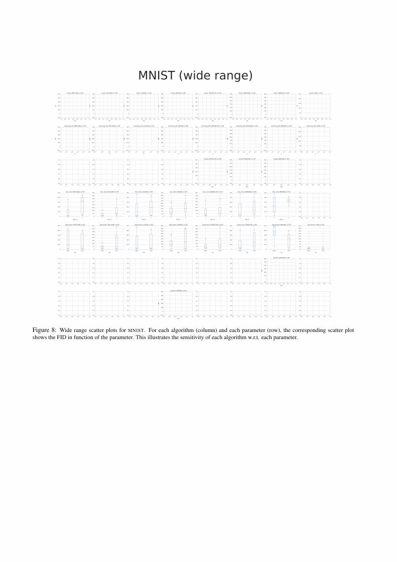
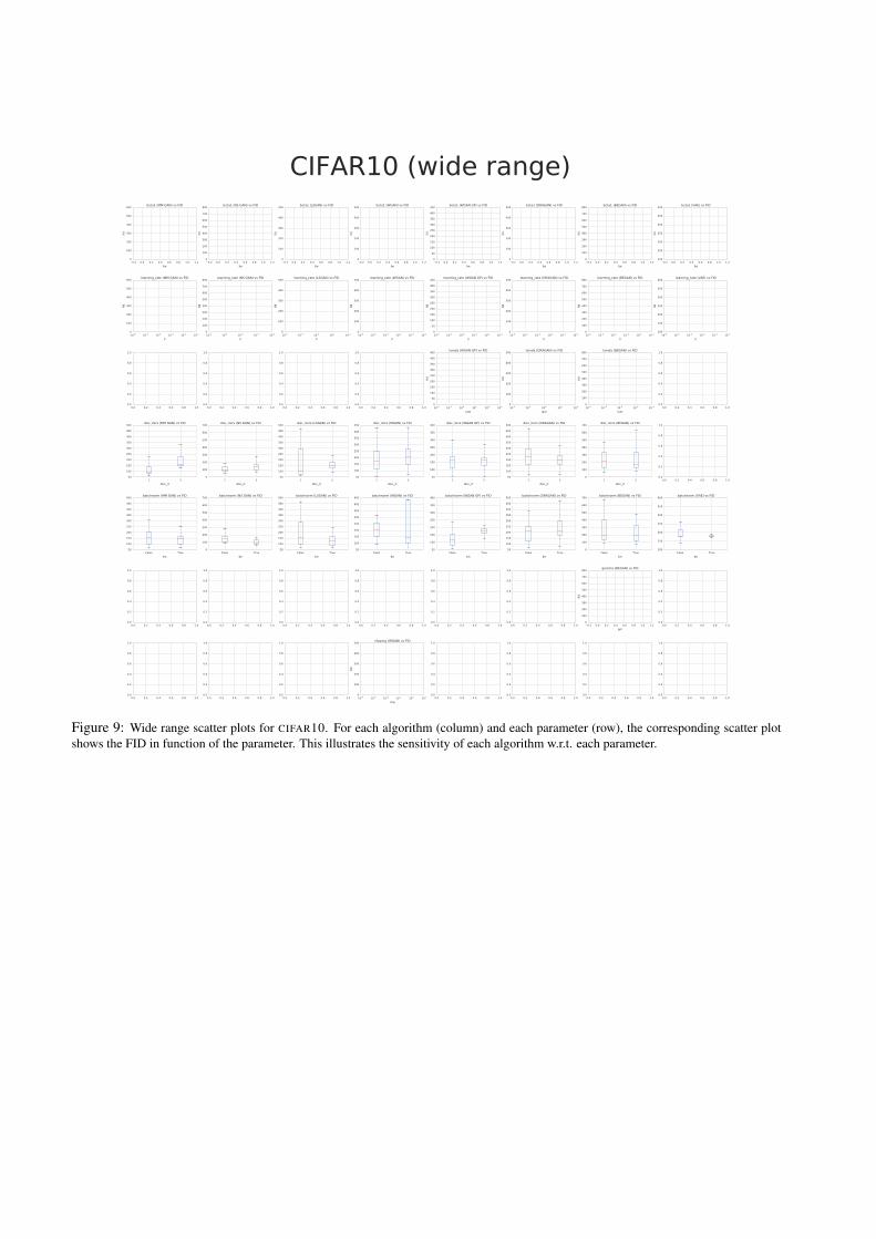
B. Which parameters really matter?Figure 7, Figure 8, Figure 9 and Figure 10 present scatter plots for data sets FASHION MNIST, MNIST, CIFAR, CELEBA

respectively. For each model and hyper-parameter we estimate its impact on the final FID. Figure 7 was used to select narrowranges of hyper-parameters.

0.2 0.0 0.2 0.4 0.6 0.8 1.0 1.2

be

0

100

200

300

400

500

600

fid

beta1 (MM GAN) vs FID

0.2 0.0 0.2 0.4 0.6 0.8 1.0 1.2

be

0

50

100

150

200

250

300

350

400

450

fid

beta1 (NS GAN) vs FID

0.2 0.0 0.2 0.4 0.6 0.8 1.0 1.2

be

0

100

200

300

400

500

fid

beta1 (LSGAN) vs FID

0.2 0.0 0.2 0.4 0.6 0.8 1.0 1.2

be

0

50

100

150

200

250

300

350

400

450

fid

beta1 (WGAN) vs FID

0.2 0.0 0.2 0.4 0.6 0.8 1.0 1.2

be

0

50

100

150

200

250

300

350

400

450

fid

beta1 (WGAN GP) vs FID

0.2 0.0 0.2 0.4 0.6 0.8 1.0 1.2

be

100

0

100

200

300

400

500

600

700

fid

beta1 (DRAGAN) vs FID

0.2 0.0 0.2 0.4 0.6 0.8 1.0 1.2

be

100

0

100

200

300

400

500

600

700

fid

beta1 (BEGAN) vs FID

0.2 0.0 0.2 0.4 0.6 0.8 1.0 1.2

be

0

50

100

150

200

250

300

fid

beta1 (VAE) vs FID

10-6 10-5 10-4 10-3 10-2 10-1

lr

0

100

200

300

400

500

600

fid

learning_rate (MM GAN) vs FID

10-6 10-5 10-4 10-3 10-2

lr

0

50

100

150

200

250

300

350

400

450

fid

learning_rate (NS GAN) vs FID

10-5 10-4 10-3 10-2 10-1

lr

0

100

200

300

400

500

fid

learning_rate (LSGAN) vs FID

10-6 10-5 10-4 10-3 10-2 10-1

lr

0

50

100

150

200

250

300

350

400

450

fid

learning_rate (WGAN) vs FID

10-6 10-5 10-4 10-3 10-2 10-1

lr

0

50

100

150

200

250

300

350

400

450

fid

learning_rate (WGAN GP) vs FID

10-6 10-5 10-4 10-3 10-2 10-1

lr

100

0

100

200

300

400

500

600

700

fid

learning_rate (DRAGAN) vs FID

10-6 10-5 10-4 10-3 10-2 10-1

lr

100

0

100

200

300

400

500

600

700

fid

learning_rate (BEGAN) vs FID

10-6 10-5 10-4 10-3 10-2 10-1

lr

0

50

100

150

200

250

300

fid

learning_rate (VAE) vs FID

0.0 0.2 0.4 0.6 0.8 1.00.0

0.2

0.4

0.6

0.8

1.0

0.0 0.2 0.4 0.6 0.8 1.00.0

0.2

0.4

0.6

0.8

1.0

0.0 0.2 0.4 0.6 0.8 1.00.0

0.2

0.4

0.6

0.8

1.0

0.0 0.2 0.4 0.6 0.8 1.00.0

0.2

0.4

0.6

0.8

1.0

10-2 10-1 100 101 102 103

lam

0

50

100

150

200

250

300

350

400

450

fid

lamda (WGAN GP) vs FID

10-2 10-1 100 101 102

lam

100

0

100

200

300

400

500

600

700

fid

lamda (DRAGAN) vs FID

10-5 10-4 10-3 10-2 10-1

lam

100

0

100

200

300

400

500

600

700

fid

lamda (BEGAN) vs FID

0.0 0.2 0.4 0.6 0.8 1.00.0

0.2

0.4

0.6

0.8

1.0

1 5

disc_it

0

100

200

300

400

500disc_iters (MM GAN) vs FID

1 5

disc_it

0

50

100

150

200

250

300

350

400

450disc_iters (NS GAN) vs FID

1 5

disc_it

0

100

200

300

400

500disc_iters (LSGAN) vs FID

1 5

disc_it

0

50

100

150

200

250

300

350

400

450disc_iters (WGAN) vs FID

1 5

disc_it

0

50

100

150

200

250

300

350

400disc_iters (WGAN GP) vs FID

1 5

disc_it

0

100

200

300

400

500

600disc_iters (DRAGAN) vs FID

1 5

disc_it

0

100

200

300

400

500

600disc_iters (BEGAN) vs FID

0.0 0.2 0.4 0.6 0.8 1.00.0

0.2

0.4

0.6

0.8

1.0

False True

bn

0

100

200

300

400

500batchnorm (MM GAN) vs FID

False True

bn

0

50

100

150

200

250

300

350

400

450batchnorm (NS GAN) vs FID

False True

bn

0

100

200

300

400

500batchnorm (LSGAN) vs FID

False True

bn

0

50

100

150

200

250

300

350

400

450batchnorm (WGAN) vs FID

False True

bn

0

50

100

150

200

250

300

350

400batchnorm (WGAN GP) vs FID

False True

bn

0

100

200

300

400

500

600batchnorm (DRAGAN) vs FID

False True

bn

0

100

200

300

400

500

600batchnorm (BEGAN) vs FID

False True

bn

50

100

150

200

250

300batchnorm (VAE) vs FID

0.0 0.2 0.4 0.6 0.8 1.00.0

0.2

0.4

0.6

0.8

1.0

0.0 0.2 0.4 0.6 0.8 1.00.0

0.2

0.4

0.6

0.8

1.0

0.0 0.2 0.4 0.6 0.8 1.00.0

0.2

0.4

0.6

0.8

1.0

0.0 0.2 0.4 0.6 0.8 1.00.0

0.2

0.4

0.6

0.8

1.0

0.0 0.2 0.4 0.6 0.8 1.00.0

0.2

0.4

0.6

0.8

1.0

0.0 0.2 0.4 0.6 0.8 1.00.0

0.2

0.4

0.6

0.8

1.0

0.2 0.0 0.2 0.4 0.6 0.8 1.0 1.2

gm

100

0

100

200

300

400

500

600

700

fid

gamma (BEGAN) vs FID

0.0 0.2 0.4 0.6 0.8 1.00.0

0.2

0.4

0.6

0.8

1.0

0.0 0.2 0.4 0.6 0.8 1.00.0

0.2

0.4

0.6

0.8

1.0

0.0 0.2 0.4 0.6 0.8 1.00.0

0.2

0.4

0.6

0.8

1.0

0.0 0.2 0.4 0.6 0.8 1.00.0

0.2

0.4

0.6

0.8

1.0

10-4 10-3 10-2 10-1 100 101

clip

0

50

100

150

200

250

300

350

400

450

fid

clipping (WGAN) vs FID

0.0 0.2 0.4 0.6 0.8 1.00.0

0.2

0.4

0.6

0.8

1.0

0.0 0.2 0.4 0.6 0.8 1.00.0

0.2

0.4

0.6

0.8

1.0

0.0 0.2 0.4 0.6 0.8 1.00.0

0.2

0.4

0.6

0.8

1.0

0.0 0.2 0.4 0.6 0.8 1.00.0

0.2

0.4

0.6

0.8

1.0

FASHION-MNIST (wide range)

Figure 7: Wide range scatter plots for FASHION MNIST. For each algorithm (column) and each parameter (row), the corresponding scatterplot shows the FID in function of the parameter. This illustrates the sensitivity of each algorithm w.r.t. each parameter. Those resultshave been used to choose the narrow range in Table 5. For example, Adam’s β1 does not seem to significantly impact any algorithm, sofor the narrow range, we fix its value to always be 0.5. Likewise, we fix the number of discriminator iterations to be always 1. For otherparameters, the selected range is smaller (e.g. learning rate), or can differ for each algorithm (e.g. batch norm).

0.2 0.0 0.2 0.4 0.6 0.8 1.0 1.2

be

100

0

100

200

300

400

500

fid


0.2 0.0 0.2 0.4 0.6 0.8 1.0 1.2

be

100

0

100

200

300

400

500

fid


0.2 0.0 0.2 0.4 0.6 0.8 1.0 1.2

be

100

0

100

200

300

400

500

fid


0.2 0.0 0.2 0.4 0.6 0.8 1.0 1.2

be

100

0

100

200

300

400

500

fid

beta1 (WGAN) vs FID

0.2 0.0 0.2 0.4 0.6 0.8 1.0 1.2

be

100

0

100

200

300

400

500

fid


0.2 0.0 0.2 0.4 0.6 0.8 1.0 1.2

be

100

0

100

200

300

400

500

600

fid


0.2 0.0 0.2 0.4 0.6 0.8 1.0 1.2

be

100

0

100

200

300

400

500

600

fid


0.2 0.0 0.2 0.4 0.6 0.8 1.0 1.2

be

0

50

100

150

200

250

fid

beta1 (VAE) vs FID

10-6 10-5 10-4 10-3 10-2 10-1

lr

100

0

100

200

300

400

500

fid


10-6 10-5 10-4 10-3 10-2

lr

100

0

100

200

300

400

500

fid


10-5 10-4 10-3 10-2 10-1

lr

100

0

100

200

300

400

500

fid


10-6 10-5 10-4 10-3 10-2 10-1

lr

100

0

100

200

300

400

500

fid


10-6 10-5 10-4 10-3 10-2 10-1

lr

100

0

100

200

300

400

500

fid


10-6 10-5 10-4 10-3 10-2 10-1

lr

100

0

100

200

300

400

500

600

fid


10-6 10-5 10-4 10-3 10-2 10-1

lr

100

0

100

200

300

400

500

600

fid


10-6 10-5 10-4 10-3 10-2 10-1

lr

0

50

100

150

200

250

fid


0.0 0.2 0.4 0.6 0.8 1.00.0

0.2

0.4

0.6

0.8

1.0

0.0 0.2 0.4 0.6 0.8 1.00.0

0.2

0.4

0.6

0.8

1.0

0.0 0.2 0.4 0.6 0.8 1.00.0

0.2

0.4

0.6

0.8

1.0

0.0 0.2 0.4 0.6 0.8 1.00.0

0.2

0.4

0.6

0.8

1.0

10-2 10-1 100 101 102 103

lam

100

0

100

200

300

400

500

fid


10-2 10-1 100 101 102

lam

100

0

100

200

300

400

500

600

fid


10-5 10-4 10-3 10-2 10-1

lam

100

0

100

200

300

400

500

600

fid


0.0 0.2 0.4 0.6 0.8 1.00.0

0.2

0.4

0.6

0.8

1.0

1 5

disc_it

0

100

200

300

400


1 5

disc_it

0

50

100

150

200

250

300

350


1 5

disc_it

0

100

200

300

400


1 5

disc_it

0

50

100

150

200

250

300

350

400


1 5

disc_it

0

50

100

150

200

250

300

350


1 5

disc_it

0

100

200

300

400


1 5

disc_it

0

100

200

300

400


0.0 0.2 0.4 0.6 0.8 1.00.0

0.2

0.4

0.6

0.8

1.0

False True

bn

0

100

200

300

400


False True

bn

0

50

100

150

200

250

300

350


False True

bn

0

100

200

300

400


False True

bn

0

50

100

150

200

250

300

350

400


False True

bn

0

50

100

150

200

250

300

350


False True

bn

0

100

200

300

400


False True

bn

0

100

200

300

400


False True

bn

20

40

60

80

100

120

140

160

180


0.0 0.2 0.4 0.6 0.8 1.00.0

0.2

0.4

0.6

0.8

1.0

0.0 0.2 0.4 0.6 0.8 1.00.0

0.2

0.4

0.6

0.8

1.0

0.0 0.2 0.4 0.6 0.8 1.00.0

0.2

0.4

0.6

0.8

1.0

0.0 0.2 0.4 0.6 0.8 1.00.0

0.2

0.4

0.6

0.8

1.0

0.0 0.2 0.4 0.6 0.8 1.00.0

0.2

0.4

0.6

0.8

1.0

0.0 0.2 0.4 0.6 0.8 1.00.0

0.2

0.4

0.6

0.8

1.0

0.2 0.0 0.2 0.4 0.6 0.8 1.0 1.2

gm

100

0

100

200

300

400

500

600

fid


0.0 0.2 0.4 0.6 0.8 1.00.0

0.2

0.4

0.6

0.8

1.0

0.0 0.2 0.4 0.6 0.8 1.00.0

0.2

0.4

0.6

0.8

1.0

0.0 0.2 0.4 0.6 0.8 1.00.0

0.2

0.4

0.6

0.8

1.0

0.0 0.2 0.4 0.6 0.8 1.00.0

0.2

0.4

0.6

0.8

1.0

10-4 10-3 10-2 10-1 100 101

clip

100

0

100

200

300

400

500

fid


0.0 0.2 0.4 0.6 0.8 1.00.0

0.2

0.4

0.6

0.8

1.0

0.0 0.2 0.4 0.6 0.8 1.00.0

0.2

0.4

0.6

0.8

1.0

0.0 0.2 0.4 0.6 0.8 1.00.0

0.2

0.4

0.6

0.8

1.0

0.0 0.2 0.4 0.6 0.8 1.00.0

0.2

0.4

0.6

0.8

1.0

MNIST (wide range)

Figure 8: Wide range scatter plots for MNIST. For each algorithm (column) and each parameter (row), the corresponding scatter plotshows the FID in function of the parameter. This illustrates the sensitivity of each algorithm w.r.t. each parameter.

0.2 0.0 0.2 0.4 0.6 0.8 1.0 1.2

be

0

100

200

300

400

500

600

fid


0.2 0.0 0.2 0.4 0.6 0.8 1.0 1.2

be

0

100

200

300

400

500

600

700

800

fid


0.2 0.0 0.2 0.4 0.6 0.8 1.0 1.2

be

0

100

200

300

400

500

fid


0.2 0.0 0.2 0.4 0.6 0.8 1.0 1.2

be

0

100

200

300

400

500

fid

beta1 (WGAN) vs FID

0.2 0.0 0.2 0.4 0.6 0.8 1.0 1.2

be

0

50

100

150

200

250

300

350

400

450

fid


0.2 0.0 0.2 0.4 0.6 0.8 1.0 1.2

be

0

100

200

300

400

500

fid


0.2 0.0 0.2 0.4 0.6 0.8 1.0 1.2

be

0

100

200

300

400

500

600

700

800

fid


0.2 0.0 0.2 0.4 0.6 0.8 1.0 1.2

be

100

150

200

250

300

350

400

fid

beta1 (VAE) vs FID

10-6 10-5 10-4 10-3 10-2 10-1

lr

0

100

200

300

400

500

600

fid


10-6 10-5 10-4 10-3 10-2

lr

0

100

200

300

400

500

600

700

800

fid


10-5 10-4 10-3 10-2 10-1

lr

0

100

200

300

400

500

fid


10-6 10-5 10-4 10-3 10-2 10-1

lr

0

100

200

300

400

500

fid


10-6 10-5 10-4 10-3 10-2 10-1

lr

0

50

100

150

200

250

300

350

400

450

fid


10-6 10-5 10-4 10-3 10-2 10-1

lr

0

100

200

300

400

500

fid


10-6 10-5 10-4 10-3 10-2 10-1

lr

0

100

200

300

400

500

600

700

800

fid


10-6 10-5 10-4 10-3 10-2 10-1

lr

100

150

200

250

300

350

400

fid


0.0 0.2 0.4 0.6 0.8 1.00.0

0.2

0.4

0.6

0.8

1.0

0.0 0.2 0.4 0.6 0.8 1.00.0

0.2

0.4

0.6

0.8

1.0

0.0 0.2 0.4 0.6 0.8 1.00.0

0.2

0.4

0.6

0.8

1.0

0.0 0.2 0.4 0.6 0.8 1.00.0

0.2

0.4

0.6

0.8

1.0

10-2 10-1 100 101 102 103

lam

0

50

100

150

200

250

300

350

400

450

fid


10-2 10-1 100 101 102

lam

0

100

200

300

400

500

fid


10-5 10-4 10-3 10-2 10-1

lam

0

100

200

300

400

500

600

700

800

fid


0.0 0.2 0.4 0.6 0.8 1.00.0

0.2

0.4

0.6

0.8

1.0

1 5

disc_it

50

100

150

200

250

300

350

400

450


1 5

disc_it

0

100

200

300

400

500

600


1 5

disc_it

50

100

150

200

250

300

350

400

450


1 5

disc_it

50

100

150

200

250

300

350

400


1 5

disc_it

50

100

150

200

250

300

350


1 5

disc_it

50

100

150

200

250

300

350

400

450


1 5

disc_it

0

100

200

300

400

500

600


0.0 0.2 0.4 0.6 0.8 1.00.0

0.2

0.4

0.6

0.8

1.0

False True

bn

50

100

150

200

250

300

350

400

450


False True

bn

0

100

200

300

400

500

600


False True

bn

50

100

150

200

250

300

350

400

450


False True

bn

50

100

150

200

250

300

350

400


False True

bn

50

100

150

200

250

300

350


False True

bn

50

100

150

200

250

300

350

400

450


False True

bn

0

100

200

300

400

500

600


False True

bn

100

150

200

250

300

350


0.0 0.2 0.4 0.6 0.8 1.00.0

0.2

0.4

0.6

0.8

1.0

0.0 0.2 0.4 0.6 0.8 1.00.0

0.2

0.4

0.6

0.8

1.0

0.0 0.2 0.4 0.6 0.8 1.00.0

0.2

0.4

0.6

0.8

1.0

0.0 0.2 0.4 0.6 0.8 1.00.0

0.2

0.4

0.6

0.8

1.0

0.0 0.2 0.4 0.6 0.8 1.00.0

0.2

0.4

0.6

0.8

1.0

0.0 0.2 0.4 0.6 0.8 1.00.0

0.2

0.4

0.6

0.8

1.0

0.2 0.0 0.2 0.4 0.6 0.8 1.0 1.2

gm

0

100

200

300

400

500

600

700

800

fid


0.0 0.2 0.4 0.6 0.8 1.00.0

0.2

0.4

0.6

0.8

1.0

0.0 0.2 0.4 0.6 0.8 1.00.0

0.2

0.4

0.6

0.8

1.0

0.0 0.2 0.4 0.6 0.8 1.00.0

0.2

0.4

0.6

0.8

1.0

0.0 0.2 0.4 0.6 0.8 1.00.0

0.2

0.4

0.6

0.8

1.0

10-4 10-3 10-2 10-1 100 101

clip

0

100

200

300

400

500

fid


0.0 0.2 0.4 0.6 0.8 1.00.0

0.2

0.4

0.6

0.8

1.0

0.0 0.2 0.4 0.6 0.8 1.00.0

0.2

0.4

0.6

0.8

1.0

0.0 0.2 0.4 0.6 0.8 1.00.0

0.2

0.4

0.6

0.8

1.0

0.0 0.2 0.4 0.6 0.8 1.00.0

0.2

0.4

0.6

0.8

1.0

CIFAR10 (wide range)

Figure 9: Wide range scatter plots for CIFAR10. For each algorithm (column) and each parameter (row), the corresponding scatter plotshows the FID in function of the parameter. This illustrates the sensitivity of each algorithm w.r.t. each parameter.

0.2 0.0 0.2 0.4 0.6 0.8 1.0 1.2

be

0

50

100

150

200

250

300

350

400

450

fid


0.2 0.0 0.2 0.4 0.6 0.8 1.0 1.2

be

0

50

100

150

200

250

300

350

400

450

fid


0.2 0.0 0.2 0.4 0.6 0.8 1.0 1.2

be

0

100

200

300

400

500

600

fid


0.2 0.0 0.2 0.4 0.6 0.8 1.0 1.2

be

0

100

200

300

400

500

fid

beta1 (WGAN) vs FID

0.2 0.0 0.2 0.4 0.6 0.8 1.0 1.2

be

0

50

100

150

200

250

300

350

400

fid


0.2 0.0 0.2 0.4 0.6 0.8 1.0 1.2

be

0

50

100

150

200

250

300

350

400

450

fid


0.2 0.0 0.2 0.4 0.6 0.8 1.0 1.2

be

0

50

100

150

200

250

300

350

400

450

fid


0.2 0.0 0.2 0.4 0.6 0.8 1.0 1.2

be

50

100

150

200

250

300

fid

beta1 (VAE) vs FID

10-6 10-5 10-4 10-3 10-2 10-1

lr

0

50

100

150

200

250

300

350

400

450

fid


10-6 10-5 10-4 10-3 10-2

lr

0

50

100

150

200

250

300

350

400

450

fid


10-5 10-4 10-3 10-2 10-1

lr

0

100

200

300

400

500

600

fid


10-6 10-5 10-4 10-3 10-2 10-1

lr

0

100

200

300

400

500

fid


10-6 10-5 10-4 10-3 10-2 10-1

lr

0

50

100

150

200

250

300

350

400

fid


10-6 10-5 10-4 10-3 10-2 10-1

lr

0

50

100

150

200

250

300

350

400

450

fid


10-6 10-5 10-4 10-3 10-2 10-1

lr

0

50

100

150

200

250

300

350

400

450

fid


10-6 10-5 10-4 10-3 10-2 10-1

lr

50

100

150

200

250

300

fid


0.0 0.2 0.4 0.6 0.8 1.00.0

0.2

0.4

0.6

0.8

1.0

0.0 0.2 0.4 0.6 0.8 1.00.0

0.2

0.4

0.6

0.8

1.0

0.0 0.2 0.4 0.6 0.8 1.00.0

0.2

0.4

0.6

0.8

1.0

0.0 0.2 0.4 0.6 0.8 1.00.0

0.2

0.4

0.6

0.8

1.0

10-2 10-1 100 101 102 103

lam

0

50

100

150

200

250

300

350

400

fid


10-2 10-1 100 101 102

lam

0

50

100

150

200

250

300

350

400

450

fid


10-5 10-4 10-3 10-2 10-1

lam

0

50

100

150

200

250

300

350

400

450

fid


0.0 0.2 0.4 0.6 0.8 1.00.0

0.2

0.4

0.6

0.8

1.0

1 5

disc_it

50

100

150

200

250

300

350

400


1 5

disc_it

50

100

150

200

250

300

350

400


1 5

disc_it

50

100

150

200

250

300

350

400

450


1 5

disc_it

0

50

100

150

200

250

300

350

400


1 5

disc_it

0

50

100

150

200

250

300

350


1 5

disc_it

0

50

100

150

200

250

300

350

400


1 5

disc_it

0

50

100

150

200

250

300

350

400


0.0 0.2 0.4 0.6 0.8 1.00.0

0.2

0.4

0.6

0.8

1.0

False True

bn

50

100

150

200

250

300

350

400


False True

bn

50

100

150

200

250

300

350

400


False True

bn

50

100

150

200

250

300

350

400

450


False True

bn

0

50

100

150

200

250

300

350

400


False True

bn

0

50

100

150

200

250

300

350


False True

bn

0

50

100

150

200

250

300

350

400


False True

bn

0

50

100

150

200

250

300

350

400


False True

bn

50

100

150

200

250


0.0 0.2 0.4 0.6 0.8 1.00.0

0.2

0.4

0.6

0.8

1.0

0.0 0.2 0.4 0.6 0.8 1.00.0

0.2

0.4

0.6

0.8

1.0

0.0 0.2 0.4 0.6 0.8 1.00.0

0.2

0.4

0.6

0.8

1.0

0.0 0.2 0.4 0.6 0.8 1.00.0

0.2

0.4

0.6

0.8

1.0

0.0 0.2 0.4 0.6 0.8 1.00.0

0.2

0.4

0.6

0.8

1.0

0.0 0.2 0.4 0.6 0.8 1.00.0

0.2

0.4

0.6

0.8

1.0

0.2 0.0 0.2 0.4 0.6 0.8 1.0 1.2

gm

0

50

100

150

200

250

300

350

400

450

fid


0.0 0.2 0.4 0.6 0.8 1.00.0

0.2

0.4

0.6

0.8

1.0

0.0 0.2 0.4 0.6 0.8 1.00.0

0.2

0.4

0.6

0.8

1.0

0.0 0.2 0.4 0.6 0.8 1.00.0

0.2

0.4

0.6

0.8

1.0

0.0 0.2 0.4 0.6 0.8 1.00.0

0.2

0.4

0.6

0.8

1.0

10-4 10-3 10-2 10-1 100 101

clip

0

100

200

300

400

500

fid


0.0 0.2 0.4 0.6 0.8 1.00.0

0.2

0.4

0.6

0.8

1.0

0.0 0.2 0.4 0.6 0.8 1.00.0

0.2

0.4

0.6

0.8

1.0

0.0 0.2 0.4 0.6 0.8 1.00.0

0.2

0.4

0.6

0.8

1.0

0.0 0.2 0.4 0.6 0.8 1.00.0

0.2

0.4

0.6

0.8

1.0

CELEBA (wide range)

Figure 10: Wide range scatter plots for CELEBA. For each algorithm (column) and each parameter (row), the corresponding scatter plotshows the FID in function of the parameter. This illustrates the sensitivity of each algorithm w.r.t. each parameter.

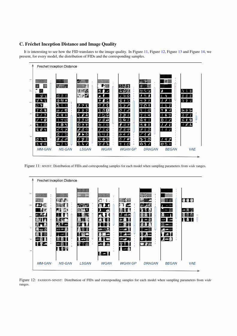
C. Frechet Inception Distance and Image QualityIt is interesting to see how the FID translates to the image quality. In Figure 11, Figure 12, Figure 13 and Figure 14, we

present, for every model, the distribution of FIDs and the corresponding samples.

Figure 11: MNIST: Distribution of FIDs and corresponding samples for each model when sampling parameters from wide ranges.

Figure 12: FASHION-MNIST: Distribution of FIDs and corresponding samples for each model when sampling parameters from wideranges.

Figure 13: CIFAR10: Distribution of FIDs and corresponding samples for each model when sampling parameters from wide ranges.

Figure 14: CELEBA: Distribution of FIDs and corresponding samples for each model when sampling parameters from wide ranges.

D. Hyper-parameter Search over Narrow RangesIn Figure 5 we presented the sensitivity of GANs to hyperparameters, assuming the samples are taken from the wide ranges

(see Table 4). For completeness, in Figure 15 we present a similar comparison for the narrow ranges of hyperparameters(presented in Table 5).

MM G

AN

NS GAN

LSGAN

WGAN

WGAN G

P

DRAGAN

BEGAN

VAE

Model

6

8

10

12

14

16

FID

Sco

re

Dataset = MNIST

MM G

AN

NS GAN

LSGAN

WGAN

WGAN G

P

DRAGAN

BEGAN

VAE

Model

20

25

30

35

40Dataset = FASHION-MNIST

MM G

AN

NS GAN

LSGAN

WGAN

WGAN G

P

DRAGAN

BEGAN

VAE

Model

50

60

70

80

90

100Dataset = CIFAR10

MM G

AN

NS GAN

LSGAN

WGAN

WGAN G

P

DRAGAN

BEGAN

VAE

Model

30

40

50

60

70

80

90

100Dataset = CELEBA

Figure 15: A narrow range search of hyperparameters which were selected based on the wide hyperparameter search on the FASHION-MNIST data set. Black stars indicate the performance of suggested hyperparameter settings. For each model we allow 50 hyperparametersamples. From the practical point of view, there are significant differences between the models: in some cases the hyperparameter rangestransfer from one data set to the others (e.g. NS GAN), while others are more sensitive to this choice (e.g. WGAN). We note that betterscores can be obtained by a wider hyperparameter search.

MM G

AN

NS GAN

LSGAN

WGAN

WGAN G

P

DRAGAN

BEGAN

VAE

Model

6

8

10

12

14

FID

Sco

re

Data set = MNIST

MM G

AN

NS GAN

LSGAN

WGAN

WGAN G

P

DRAGAN

BEGAN

VAE

Model

15

20

25

30

35

40Data set = FASHION-MNIST

MM G

AN

NS GAN

LSGAN

WGAN

WGAN G

P

DRAGAN

BEGAN

VAE

Model

50

55

60

65

70

75

80Data set = CIFAR10

MM G

AN

NS GAN

LSGAN

WGAN

WGAN G

P

DRAGAN

BEGAN

VAE

Model

20

30

40

50

60

70

80

90

100Data set = CELEBA

Figure 16: For each model we search for best hyperparameters on the wide range. Then, we retrain each model using the best parameters50 times with random initialization of the weights, keeping everything else fixed. We observe a slight variance in the final FID. Hence,when an FID is reported it is paramount that one compares the entire distribution, instead of the best seed for the best run. The figurecorresponds to Table 3.

E. Precision, Recall and F1 as a Function of the Budget

5 10 15 20 25 30 35 40 45 50 55 60 65 70

Budget

0.2

0.0

0.2

0.4

0.6

0.8

1.0

1.2

Valu

e

Measure = F1

5 10 15 20 25 30 35 40 45 50 55 60 65 70

Budget

0.2

0.4

0.6

0.8

1.0

Measure = Precision

5 10 15 20 25 30 35 40 45 50 55 60 65 70

Budget

0.2

0.0

0.2

0.4

0.6

0.8

1.0

1.2Measure = Recall

Model

BEGAN

DRAGAN

MM GAN

NS GAN

WGAN

WGAN GP

Figure 17: Optimizing for F1, threshold δ = 1.0.

5 10 15 20 25 30 35 40 45 50 55 60 65 70

Budget

0.1

0.0

0.1

0.2

0.3

0.4

0.5

Valu

e

Measure = F1

5 10 15 20 25 30 35 40 45 50 55 60 65 70

Budget

0.2

0.4

0.6

0.8

1.0

Measure = Precision

5 10 15 20 25 30 35 40 45 50 55 60 65 70

Budget

0.05

0.00

0.05

0.10

0.15

0.20

0.25

0.30

0.35Measure = Recall

Model

BEGAN

DRAGAN

MM GAN

NS GAN

WGAN

WGAN GP

Figure 18: Optimizing for F1, threshold δ = 0.5.

5 10 15 20 25 30 35 40 45 50 55 60 65 70

Budget

0.2

0.0

0.2

0.4

0.6

0.8

1.0

Valu

e

Measure = F1

5 10 15 20 25 30 35 40 45 50 55 60 65 70

Budget

0.60

0.65

0.70

0.75

0.80

0.85

0.90

0.95

1.00


5 10 15 20 25 30 35 40 45 50 55 60 65 70

Budget

0.2

0.0

0.2

0.4

0.6

0.8

1.0Measure = Recall

Model

BEGAN

DRAGAN

MM GAN

NS GAN

WGAN

WGAN GP

Figure 19: Optimizing for precision, threshold δ = 1.0.

5 10 15 20 25 30 35 40 45 50 55 60 65 70

Budget

0.05

0.00

0.05

0.10

0.15

0.20

0.25

Valu

e

Measure = F1

5 10 15 20 25 30 35 40 45 50 55 60 65 70

Budget

0.2

0.4

0.6

0.8

1.0

Measure = Precision

5 10 15 20 25 30 35 40 45 50 55 60 65 70

Budget

0.02

0.00

0.02

0.04

0.06

0.08

0.10

0.12

0.14


Model

BEGAN

DRAGAN

MM GAN

NS GAN

WGAN

WGAN GP

Figure 20: Optimizing for precision, threshold δ = 0.5.

5 10 15 20 25 30 35 40 45 50 55 60 65 70

Budget

0.2

0.0

0.2

0.4

0.6

0.8

1.0

Valu

e

Measure = F1

5 10 15 20 25 30 35 40 45 50 55 60 65 70

Budget

0.2

0.0

0.2

0.4

0.6

0.8

1.0


5 10 15 20 25 30 35 40 45 50 55 60 65 70

Budget

0.2

0.0

0.2

0.4

0.6

0.8

1.0

1.2Measure = Recall

Model

BEGAN

DRAGAN

MM GAN

NS GAN

WGAN

WGAN GP

Figure 21: Optimizing for recall, threshold δ = 1.0.

5 10 15 20 25 30 35 40 45 50 55 60 65 70

Budget

0.1

0.0

0.1

0.2

0.3

0.4

0.5

Valu

e

Measure = F1

5 10 15 20 25 30 35 40 45 50 55 60 65 70

Budget

0.2

0.4

0.6

0.8

1.0

Measure = Precision

5 10 15 20 25 30 35 40 45 50 55 60 65 70

Budget

0.05

0.00

0.05

0.10

0.15

0.20

0.25

0.30


Model

BEGAN

DRAGAN

MM GAN

NS GAN

WGAN

WGAN GP

Figure 22: Optimizing for recall, threshold δ = 0.5.

F. Does the Solver Matter?We ran the WGAN training across 100 hyperparameter settings. In the first set of experiments we used the ADAM

optimizer, and in the second the RMSPROP optimizer. We observe that distribution of the scores is similar and it’s unclearwhich optimizer is ”better”. However, on both data sets ADAM outperformed RMSPROP on recommended parameters(CIFAR10: 154.5 vs 161.2, CELEBA: 97.9 vs 216.3) which highlights the need for a hyperparameter search. As a result, theconclusions of this work are not altered by this choice.

Are GANs Created Equal? A Large-Scale Study · PDF fileAre GANs Created Equal? A Large-Scale...

Documents

Transcript of Are GANs Created Equal? A Large-Scale Study · PDF fileAre GANs Created Equal? A Large-Scale...