WP/04/141

Are Developing Countries Better Off Spending Their Oil Wealth Upfront?

Hajime Takizawa

Edward H. Gardner Kenichi Ueda

© 2004 International Monetary Fund WP/04/141

IMF Working Paper

Middle East and Central Asia Department and Research Department

Are Developing Countries Better Off Spending Their Oil Wealth Upfront?

Prepared by Hajime Takizawa, Edward H. Gardner, and Kenichi Ueda1

August 2004

Abstract

This Working Paper should not be reported as representing the views of the IMF. The views expressed in this Working Paper are those of the author(s) and do not necessarily represent those of the IMF or IMF policy. Working Papers describe research in progress by the author(s) and are published to elicit comments and to further debate.

We question the conventional view that it is optimal for government to maintain a stable level of spending out of oil wealth. We compare this conventional policy recommendation with one where government spends all of its oil revenues upfront, at the same rate as oil is extracted. Using a neoclassical growth model with positive external effects of public spending on consumption and productivity, we find that, if the economy is growing along the steady-state balanced path, the conventional view is validated. However, if the economy starts with a lower capital stock, the welfare ranking across two policies can be reversed. JEL Classification Numbers: O23, Q32 Keywords: Optimal fiscal policy, public investment, transitional growth, natural resource Author’s E-Mail Address: htakizawa@imf.org; egardner@imf.org; kueda@imf.org

1 Economist, Middle East and Central Asia Department, IMF; Division Chief, Middle East and Central Asia Department, IMF; and Economist, Research Department, IMF, respectively. The authors are grateful to Mohsin Khan, Ashoka Mody, Aasim Husain, Jean Le Dem, and Jacques Bouhga-Hagbe for their valuable comments. All remaining errors are our own.

- 2 -

Contents Page

I. Introduction .................................................................................................................. 3 II. The Model .................................................................................................................... 5 A. The Economy ......................................................................................................... 5 B. Competitive Equilibrium of the Economy ........................................................... 11 III. Results of Simulation Exercises................................................................................. 13 A. Some Considerations in Characterizing Equilibria .............................................. 13 B. The Baseline Economy......................................................................................... 13 C. Fiscal Policy Rules and Simulation Results ......................................................... 15 IV. Conclusions................................................................................................................ 19 Appendix ................................................................................................................................ 21 References .............................................................................................................................. 28 Tables 1. Parameter Values for the Baseline Economy............................................................. 15 2. Welfare Comparisons................................................................................................. 17 Figures 1. Comparison between the Hand-to-Mouth Policy and the Annuity Policy on a Balanced Growth Path (Example 1)......................................................................... 26 2. Comparison between the Hand-to-Mouth Policy and Annuity Policy on a Transitional Path (Example 2) ................................................................................. 27

- 3 -

I. INTRODUCTION The literature on optimal fiscal policy in countries endowed with exhaustible natural resources (oil, for simplicity) has typically been based on the premise that government spending is akin to consumption. Drawing from the classical paper by Hotelling (1931) and a more modern treatment by Romer (1986), the literature has essentially looked at the government’s problem as one of optimizing the intertemporal allocation of that consumption. Within this framework, intergenerational welfare maximization typically produces variants of a permanent consumption rule, where oil wealth is gradually transformed into financial wealth whose income stream sustains a stable level of government spending. This paper introduces another dimension to the government’s fiscal choice by assuming that government spending contains both an investment and a consumption component. This establishes an explicit link between government spending and productivity. In this expanded framework, government spending affects not only the welfare of the current generation, because of the consumption value of government spending, but also that of future generations, because of the impact of government spending on productivity and the incentives it creates for private capital accumulation. This interpretation of government spending is consistent with the broadly shared view that government spending on social (e.g., health and education) and physical infrastructure does in fact raise productivity and private investment. This is also the basis for the claim by governments in resource-rich developing countries that they should spend more of the resource endowment upfront, when the marginal benefit of government spending is likely to be higher than the return from external financial assets. Finding an analytical solution to the welfare maximization problem in this expanded model proves to be very difficult, and thus we opt for a numerical approach. We explore whether and how the welfare ranking of two simple policy rules in an economy with finite and declining oil revenues is affected by initial conditions and assumptions about the consumption and investment value of public spending. The policy rules we examine are: (i) the hand-to-mouth rule, under which the government spends the bulk of oil revenues as they accrue, thus favoring current spending over future spending; and (ii) the annuity rule, under which the government maintains a constant real per capita level of spending by transforming oil wealth into financial assets. The latter policy rule approximates the optimal solution typically found in the literature. We find that, when the economy grows along the steady-state balanced growth path, the conventional view is validated under standard assumptions about the production technology and the utility function: namely, the annuity policy yields a higher welfare than the hand-to-mouth policy rule. However, when the economy is on the transition path because of low initial capital stocks, as would be the case in developing countries, the welfare ranking across the two policies can be reversed, depending on the contribution of government spending to output growth.

- 4 -

This is not a trivial result, in that it does not simply follow from the fact that the rate of return from public investment exceeds that from financial assets when the initial capital stock is low. For future generations, the annuity policy is always better than the hand-to-mouth policy, because of the higher level of government spending that can be sustained in steady state. However, the hand-to-mouth policy can be welfare improving for a capital-scarce economy if the benefits of a faster convergence to steady state outweigh the losses of lower government spending in the steady state. The productivity-enhancing effects of government spending (investment) also depend on the quality or efficiency of that spending. This effect is modeled in the paper through an efficiency parameter. The analysis in this paper follows the tradition of the literature on dynamic optimal fiscal policy in which the government optimizes people’s welfare over time using fiscal policy tools.2 However, to our knowledge, this is the first formal analysis of the growth-enhancing effects of government spending that explicitly and formally looks at transitional dynamics to a steady state and their impact on welfare. Although the presence of exhaustible resources is central to the analysis, the issue of optimal intertemporal allocation of government spending raised in the paper has general applicability. In as much as government affects the growth path, it will also change its intertemporal budget constraint. However, these considerations take on much greater weight in resource-rich countries because of the greater latitude these countries enjoy in front-loading spending without incurring debt or facing the discipline of financial markets. Evidence of externalities of public goods on the production side can be found in various empirical studies. Cross country studies find that government’s development spending, a proxy for public capital stock, has positive effects on growth. Easterly and Rebelo (1993) find correlation between general government investment (as well as investment in transport and communications) and growth for low-income countries. The finding has been reconfirmed by subsequent studies including Gupta and others (2002) for low-income countries; Ueda and Parrado (2003) for small island countries; and Kneller, Bleaney, and Gemmel (1999, 2000) for OECD countries. There is also a strand of the empirical literature on growth models that takes into account growth-enhancing effect of public investment. Using an endogenous growth model with panel data for 23 industrial countries, Cashin (1995) finds a growth-enhancing effect of investment in public capital. Miller and Tsoukis (2001) reach a similar conclusion by testing a model in which both exogenous and endogenous growth models are nested. Some studies use a neoclassical growth model that is augmented to distinguish between public and private capital to estimate the impact of private and public sector investment on growth. Results of those studies are somewhat mixed. Aschauer (1989, 1998) finds that investment in infrastructure had a positive effect on productivity in the United States and Mexico. Using a cross-section sample of developing countries, Khan and Reinhart (1990) and Khan and 2 A seminal paper is Lucas and Stokey (1983). For a more recent treatment, see Barro and Sala-i-Martin (1995).

- 5 -

Kumar (1997) compare the effect of public and private investment on long-run growth and find that private investment has a larger direct effect. The remainder of the paper is organized as follows. Section II develops a model and defines a competitive equilibrium. Section III characterizes competitive equilibria of various economies to derive welfare implications of spending policies. Section IV concludes. The Appendix provides discussion on details of the model.

II. THE MODEL This section develops a model to analyze how alternative government spending paths, out of exhaustible natural resource revenues, affect the welfare of the economy in a decentralized competitive setting. We use a variant of the standard neoclassical growth model, in which private agents maximize welfare by allocating income between consumption and investment. Oil resources belong to the governments and are extracted at a predetermined and declining rate. Government spending affects both productivity of private capital and private utility, and the fiscal policy rule defines exante the pattern of spending over time. We do not model explicitly the choice between government consumption and government investment but assume that the consumption and investment contents of government spending are given, and examine how changes in this assumption affect the welfare ranking of the two spending rules.3 While the government has access to external financial assets to reallocate spending across time, private agents are assumed to operate in a closed economy, with physical capital as the only instrument available for intertemporal consumption smoothing. We believe (as discussed below) that this seemingly restrictive assumption is in fact quite realistic and that its relaxation would not alter the main conclusions of the paper.

A. The Economy The economy is populated by a large number of consumer-worker-investor households indexed by [0,1]η∈ . The measure of households is normalized to unity. The size of each household grows at an exogenous rate n. Hence, n represents the growth rate of the population. The economy is also populated by a single firm which takes prices as given in making its decisions.4 The government announces and commits to its fiscal policy for future dates. Households and the firm make their decisions after observing the announced fiscal policy. Timing of events in the economy is discrete, and no uncertainty exists. At the start of each period, the households rent their capital and labor services to the firm. The firm employs 3 We use the word spending to denote the use of real resources, even though part of government spending should in fact be considered as saving, in as much as it increases the public capital stocks.

4 The assumption of a single firm is made to simplify presentation, but it does not alter the results.

- 6 -

them and uses public capital available for free to produce a single consumption-capital good. At the end of the period, after production has occurred, the firm returns the undepreciated portion of the capital stock to the households and also makes rental payments for the use of production factors. All income payments to the households are taxed by the government at a flat rate. In addition, exhaustible resources endowed to the economy yield non-tax revenues to the government.5 Following the distribution of incomes, households use their after-tax incomes to purchase consumption and investment goods from the firm. The government purchases single consumption-investment goods from the firm and also imports the same goods from abroad if the supply from the domestic firm falls short of the government’s demand. The government uses the purchased goods to provide goods and services to the households and to make investment in public capital. The government’s net financial position is fully reflected in changes in the government’s net external assets. Finally, the undepreciated private capital plus the new investment goods are carried over by the households into the following period. The undepreciated public capital plus the new investment goods purchased by the government are similarly carried over into the following period. Income is taxed at a constant rate, and the tax parameter is not used as a policy instrument to maximize welfare. In the model, only the government has access to foreign capital markets. By contrast, households cannot save into foreign financial assets or borrow from abroad. By implication, the economy’s external current account balance equals the fiscal balance. We would argue that this seemingly arbitrary assumption is in fact not unrealistic for developing resource-rich economies. If the economy were open, sizable capital inflows (private current account deficits) would be observed on the convergence path toward steady-state growth, taking advantage of the fact that domestic assets carry a higher rate of return than foreign assets. This theoretical prediction is common to all the neoclassical growth models but is counterfactual—known as the Lucas puzzle (Lucas, 1990). Because this paper does not intend to solve this puzzle, a simple closed-economy assumption for households is adopted. Moreover, in our numerical examples, the government only accumulates or draws down foreign financial assets and is therefore not bound by any borrowing constraint. The model ignores the possibility of domestic saving by the government in the form of investing in and then renting private capital. Such an extension of the model would not change the results, in as much as private sector behavior would adjust to restore the original equilibrium. The firm A constant-returns-to-scale production technology is available for the firm to transform labor input, f

th , private capital, ,fp tk , and economy-wide public capital normalized by economy-

5 For computational simplicity, the natural resources sector is assumed to employ no domestic production factors. While this will not be entirely realistic, it is a good approximation for oil-rich countries, many of which rely on foreign capital and labor for exploration, development and extraction activities, with the government collecting part of the rents.

- 7 -

wide labor input, , /g t tK H , into a consumption-capital good, where ,g tK and tH are

economy-wide public capital stock and labor input, respectively. Inputs, fth and ,

fp tk , are

under the direct control of the firm, while an economy-wide variable, , /g t tK H , is outside the control of the firm. Here, and throughout the paper, the superscript f indicates quantities chosen by the firm, while the subscript t indicates quantities either in period t (in the case of flow variables) or at the beginning of period t (in the case of stock variables). The subscripts p and g indicate variables chosen by the private sector and the government, respectively. Uppercase and lowercase variables represent aggregate and individual (both firm and household) variables, respectively. In what follows, the following Cobb-Douglas production function is assumed:

( )1 α

α,, , ,( , ; , ) θ ,g tf f f f

p t t g t t t t t p tt

Kf k h K H A h k

H

−

= + (1)

where α (0,1)∈ is the income share of private capital, tθ (0,1)∈ represents the degree of efficiency in the use of public capital, and 0tA > represents the technology level. The technology level is assumed to grow at a constant rate, γ, that is exogenous to the economy.

One of the reasons that production depends not on the absolute level of the economy-wide public capital, ,g tK , but on the normalized public capital, , /g t tK H , is to capture congestion effects. The assumption implies that the higher the level of economic activity (approximated by the economy-wide labor input) is, the larger is the public capital stock required to maintain its efficiency in production.6 Another reason for normalizing public capital is that it ensures consistency of the model with balanced growth in steady state, one of the stylized facts of economic growth documented by Kaldor (1963).7 The model exhibits balanced growth in that, in steady state, private capital, public capital, and output grow at a constant rate8 (1 )(1 ) 1nγ+ + − driven by the exogenous productivity growth 1 γ+ and the exogenous population growth 1 n+ . 6 This congestion effect in the use of public goods is also analyzed by Barro and Sala-i-Martin (1992; 1995, pp. 158–59).

7 Also see Cooley and Prescott (1995).

8 That the production function is consistent with balanced growth can be confirmed by multiplying At by (1 )γ+ , ht and tH by (1 )n+ , and kp,t and ,g tK by (1 )(1 )nγ+ + in the production function. It is straightforward to confirm that output grows at the rate (1 )(1 ) 1nγ+ + − .

- 8 -

The optimal behavior of the firm can be derived as a solution to the maximization of period-by-period profit:

, , , , ,, , , , , , , , ,

{ , , , , , }

, , , , , ,

max ( , ) ( , )

s.t. ( , ; , ),

f f f f f fp t g t p t g t p t t

f f f f f fp t g t p t g t p t g t p t p t g t t

c c i i k h

f f f f f fp t g t p t g t p t t g t t

c c i i r K K k w K K h

c c i i f k h K H

+ + + − ⋅ − ⋅

+ + + ≤ (2)

where ,

fp tc and ,

fg tc represent consumption by households and the government, respectively,

and ,fp ti and ,

fg ti represent investment by households and the government, respectively. Rental

rate , ,( , )p t g tr K K and wage rate , ,( , )p t g tw K K are functions of aggregate economy-wide private capital and aggregate economy-wide public capital. The maximization requires that marginal returns of inputs be equal to marginal products:

, , , ,, ,

, ,

( , ; , ) ( , ; , )( , )

f f f fp t t g t t p t t g t t

t p t g t f fp t p t

f k h K H f k h K Hr K K

k kα

∂= =

∂, (3)

and

, , , ,, ,

( , ; , ) ( , ; , )( , ) (1 )

f f f fp t t g t t p t t g t t

t p t g t f ft t

f k h K H f k h K Hw K K

h hα

∂= = −

∂. (4)

Households Both private purchases cp,t and government purchases of the consumption good cg,t enter into each household’s utility function, as follows:

, ,0

( , )tp t g t

tu c cβ

∞

=∑ , (5)

where , ,( , )p t g tu c c is an isoelastic utility function and β is the discount factor. The households are both workers and own private capital. They provide labor services and capital to the firm. Available time for labor in period t is denoted by th . Furthermore, th in period 0t = is normalized to unity. Private capital owned by a household is denoted by ,p tk . Since the household’s preference does not depend on the number of hours worked, households inelastically provide labor services. Given the capital stock held by individual households at the beginning of period t, ,p tk , aggregate economy-wide capital held in total by all households can be defined by

1

, ,0p t p tK k dη= ∫ . Similarly, aggregate economy-wide labor input is defined by 1

0t tH h dη= ∫ .

The households receive factor payments from the firm, but taxes are collected at a uniform tax rate tτ . After-tax income is equal to , , , , ,( , ) ( , ) (1 )t p t g t t t p t g t p t tw K K h r K K k τ ⋅ + ⋅ − .

- 9 -

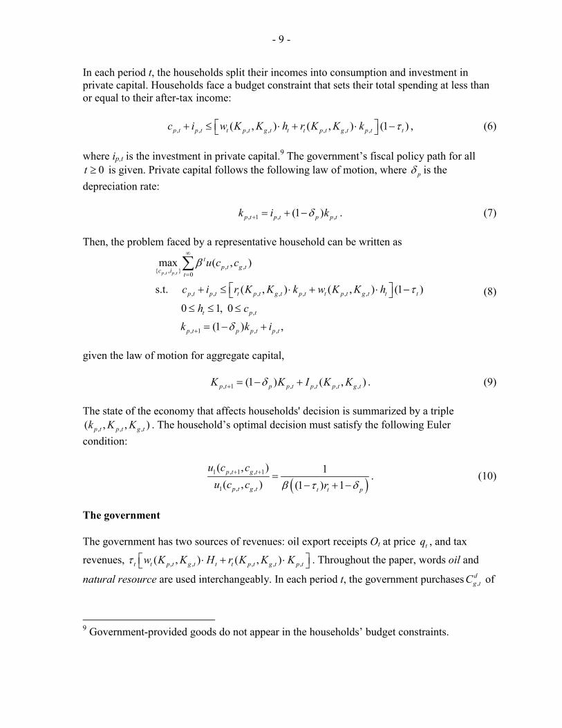
In each period t, the households split their incomes into consumption and investment in private capital. Households face a budget constraint that sets their total spending at less than or equal to their after-tax income: , , , , , , ,( , ) ( , ) (1 )p t p t t p t g t t t p t g t p t tc i w K K h r K K k τ + ≤ ⋅ + ⋅ − , (6) where ip,t is the investment in private capital.9 The government’s fiscal policy path for all

0t ≥ is given. Private capital follows the following law of motion, where pδ is the depreciation rate: , 1 , ,(1 )p t p t p p tk i kδ+ = + − . (7) Then, the problem faced by a representative household can be written as

, ,, ,{ , } 0

, , , , , , ,

,

, 1 , ,

max ( , )

s.t. ( , ) ( , ) (1 )

0 1, 0

(1 ) ,

p t p t

tp t g tc i t

p t p t t p t g t p t t p t g t t t

t p t

p t p p t p t

u c c

c i r K K k w K K h

h c

k k i

β

τ

δ

∞

=

+

+ ≤ ⋅ + ⋅ − ≤ ≤ ≤

= − +

∑

(8)

given the law of motion for aggregate capital, , 1 , , , ,(1 ) ( , )p t p p t p t p t g tK K I K Kδ+ = − + . (9) The state of the economy that affects households' decision is summarized by a triple

, , ,( , , )p t p t g tk K K . The household’s optimal decision must satisfy the following Euler condition:

( )1 , 1 , 1

1 , ,

( , ) 1( , ) (1 ) 1p t g t

p t g t t t p

u c cu c c rβ τ δ

+ + =− + −

. (10)

The government The government has two sources of revenues: oil export receipts Ot at price tq , and tax

revenues, , , , , ,( , ) ( , )t t p t g t t t p t g t p tw K K H r K K Kτ ⋅ + ⋅ . Throughout the paper, words oil and

natural resource are used interchangeably. In each period t, the government purchases ,dg tC of

9 Government-provided goods do not appear in the households’ budget constraints.

- 10 -

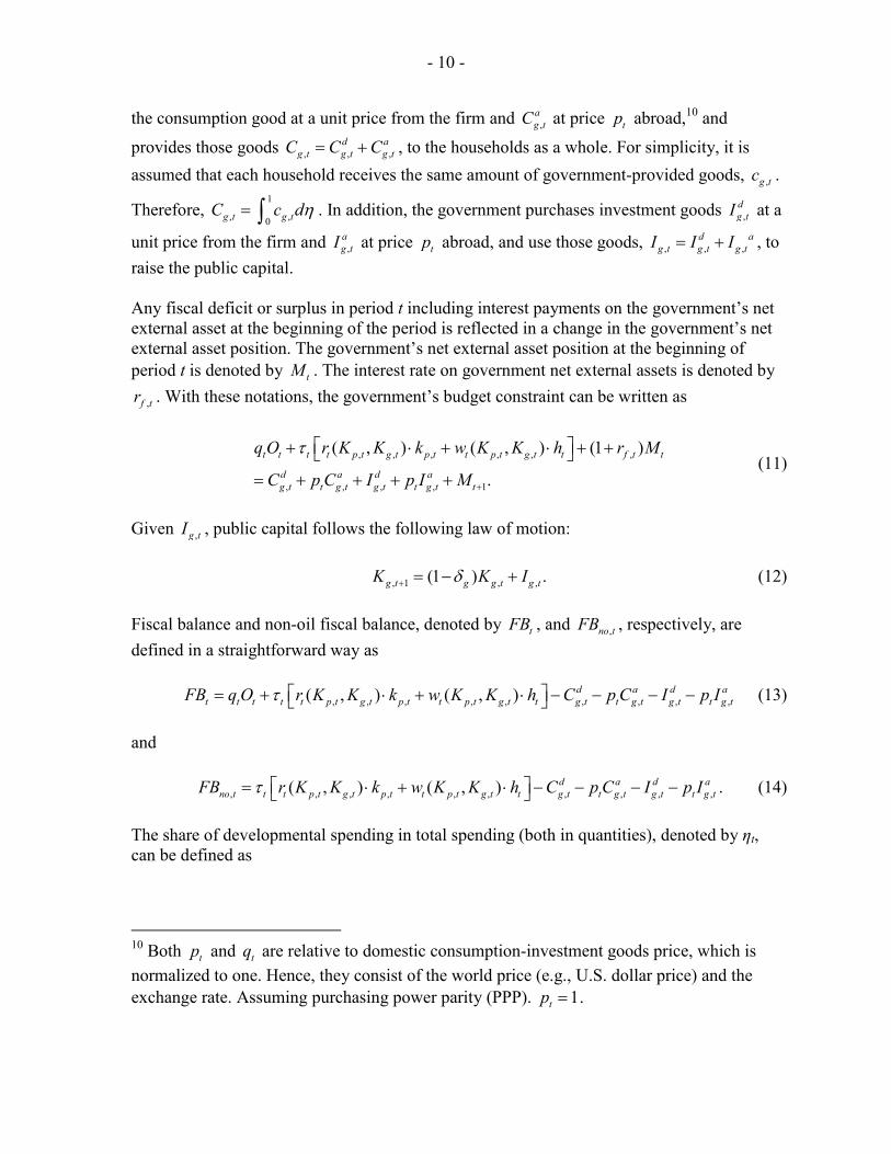
the consumption good at a unit price from the firm and ,ag tC at price tp abroad,10 and

provides those goods , , ,d a

g t g t g tC C C= + , to the households as a whole. For simplicity, it is assumed that each household receives the same amount of government-provided goods, ,g tc .

Therefore, 1

, , 0g t g tC c dη= ∫ . In addition, the government purchases investment goods ,dg tI at a

unit price from the firm and ,ag tI at price tp abroad, and use those goods, , , ,

d ag t g t g tI I I= + , to

raise the public capital. Any fiscal deficit or surplus in period t including interest payments on the government’s net external asset at the beginning of the period is reflected in a change in the government’s net external asset position. The government’s net external asset position at the beginning of period t is denoted by tM . The interest rate on government net external assets is denoted by

,f tr . With these notations, the government’s budget constraint can be written as

, , , , , ,

, , , , 1

( , ) ( , ) (1 )

.t t t t p t g t p t t p t g t t f t t

d a d ag t t g t g t t g t t

q O r K K k w K K h r M

C p C I p I M

τ

+

+ ⋅ + ⋅ + + = + + + +

(11)

Given ,g tI , public capital follows the following law of motion: , 1 , ,(1 ) .g t g g t g tK K Iδ+ = − + (12) Fiscal balance and non-oil fiscal balance, denoted by tFB , and ,no tFB , respectively, are defined in a straightforward way as , , , , , , , , ,( , ) ( , ) d a d a

t t t t t p t g t p t t p t g t t g t t g t g t t g tFB q O r K K k w K K h C p C I p Iτ = + ⋅ + ⋅ − − − − (13) and , , , , , , , , , ,( , ) ( , ) d a d a

no t t t p t g t p t t p t g t t g t t g t g t t g tFB r K K k w K K h C p C I p Iτ = ⋅ + ⋅ − − − − . (14) The share of developmental spending in total spending (both in quantities), denoted by ηt, can be defined as

10 Both tp and tq are relative to domestic consumption-investment goods price, which is normalized to one. Hence, they consist of the world price (e.g., U.S. dollar price) and the exchange rate. Assuming purchasing power parity (PPP). 1tp = .

- 11 -

,

, ,

g tt

g t g t

II C

η =+

. (15)

Resource constraint The economy’s external current account balance is, by construction, the same as its fiscal balance. While the sum of households’ after-tax incomes and tax revenues is equal to domestic non-oil output, the sum of households’ spending and the government’s spending is not necessarily equal to the non-oil output of the economy because of oil revenues and changes in government net external assets. In other words, saving must be equal to investment for the households but not for the government. Consequently, the economy-wide net external asset is simply the government’s net external asset. Since the current account balance determines how much resources the economy can use, the definition of the current account balance is also the resource constraint of the economy. The current account balance of the economy, tCA , is equal to the oil revenue plus the non-oil output minus the spending by the households and the government: , , , , , , ,( , ; , ) d a d a

t t t p t t g t p t g t t g t p t g t t g tCA q O f K H K H C C p C I I p I= + − − − − − − . (16) The non-oil current account balance, ,no tCA , is defined in a similar manner: , , , , , , , ,( , ; , ) d a d a

no t p t t g t p t g t t g t p t g t t g tCA f K H K H C C p C I I p I= − − − − − − . (17) Given tFB or tCA , net external asset evolves as follows:

1 ,

,

(1 )

(1 ) .t f t t t

f t t t

M r M FB

r M CA+ = + +

= + + (18)

B. Competitive Equilibrium of the Economy

This section defines competitive equilibrium of the economy. The equilibrium defined here is computed for various economies in the next section.

Definition 1. Competitive Equilibrium. Given an interest rate on net external assets, ,f tr , a

government’s policy, , , , , ,{ , , , , , , }d a d at g t g t g t g t g t tc c K I I Mτ , and world prices of an imported

consumption-investment good tp and of oil tq , a competitive equilibrium of the economy is defined by a set of domestic prices{ , }t tr w , an allocation of resources , , ,{ , , , }p t p t p t tc i k h , and the aggregate investment function, , , ,( , )p t p t g tI K K , such that

(i) all markets clear—that is,

- 12 -

1

, , , 0( )f

p t t p t p tk K k d kη= = =∫ ,

1

, , , , 0( )f

p t p t p t p tc C c d cη= = =∫ ,

1

01 ( 1)f

t t t th H h d hη= = = = =∫ ,

1

, , , , 0( )f

p t p t p t p ti I i d iη= = =∫ ;

(ii) prices and quantities solve the consumer’s problem (8) given the law of motion for aggregate private capital (9);

(iii) prices and quantities satisfy the first order necessary conditions of the firm’s profit maximization (3) and (4);

(iv) the aggregate resource constraint, equation (16), is satisfied; and

(v) the aggregate investment function assumed by the households, , , ,( , )p t p t g tI K K , coincides with what individual households actually plan to invest in the aggregate, based on the individual household’s decision function, , , , , ,( , , )p t p t p t p t g ti i k K K= % , evaluated at , ,p t p tk K= .

Definition 1 automatically implies the government budget constraint (11) because of the equivalence between the fiscal balance and the current account balance. Mechanically, this result follows from the constant-return-to-scale property of the production function—that is, the fact that all factor payments exhaust non-oil output. Because of the constant-return-to-scale property of the production function, combining the budget constrain of the households and the government results in the definition of the current account balance in equation (16).

Economic welfare is measured by the sum of a discounted utility stream (5) evaluated at a competitive equilibrium. The measure of the welfare is a function of initial private capital,

,p tk for 0t = . Accordingly, the welfare loss or gain arising from changes in fiscal policy can be measured by the amount of private capital, normalized by non-oil output, necessary to compensate for the welfare loss or gain.11, 12 Welfare comparisons in the rest of the paper are carried out using this metric.

11 For a given economy, non-oil output in the initial period is the same under any policies because labor input, initial private capital, and initial public capital of the economy are the same.

12 Welfare loss is typically measured by necessary compensations by consumption (see, for example, Lucas (2000)). Applying this approach to growth model with transition path, however, is questionable because the consumption path adjusted for the compensation is not necessarily the optimal choice of the households any more. On the other hand, measuring the welfare loss or gain by the necessary compensation in initial private capital is immune to this deviation from the optimal path. See Townsend and Ueda (2001) for welfare comparison by

(continued…)

- 13 -

III. RESULTS OF SIMULATION EXERCISES

A. Some Considerations in Characterizing Equilibria

Under the standard assumptions of neoclassical growth models, the model economy converges to a unique balanced growth path regardless of initial conditions. All simulations considered in this paper satisfy this convergence property. However, welfare depends not only on the balanced growth properties of the economy but also on the characteristics of the transitional convergence path to a balanced growth path. The characteristics of transitional paths depend on initial conditions and policy choices. The paper limits its attention to fiscal policy rules that are consistent with a constant net external asset positions in steady state, by requiring balanced budgets along the steady state growth path. This restriction ensures fiscal sustainability and makes it possible to carry out meaningful welfare comparisons across simulations.

B. The Baseline Economy This section describes a baseline economy. All extensions in the later sections are variants. Henceforth, all variables are de-trended by their respective growth rates on the balanced growth path so that they converge to constant levels in the steady state. A functional form for the household’s preference builds on a standard utility function used in the study of business cycles and economic growth in dynamic general equilibrium models. In particular, the following functional form is assumed:

( )11

, ,, ,( , )

1p t g t

p t g t

c cu c c

σλ λ

σ

−−

=−

. (19)

The inverse of the parameter σ represents the intertemporal elasticity of substitution and represents the degree to which consumption will be postponed (to the next period) in response to additional rewards (i.e., a rise in the interest rate). The lower the sensitivity, the greater is the desire of households to maintain a constant level of consumption over time. The parameter λ represents the weight of private consumption in the household utility function. Government spending potentially affects the welfare of the economy through two channels: the growth-enhancing effect of public capital and the direct provision of consumption goods. In order to study separately these two channels, we begin by assuming (in the baseline economy) that 1λ = in the baseline economy. Setting 1λ = shuts down the

wealth transfer based on a value function comparison in a transitional growth model and Burdick (1997) for a different approach.

- 14 -

second channel, meaning that all nondevelopmental spending by the government is effectively a waste of resources. Structural parameters are set at realistic values found in the literature. The inverse of the intertemporal elasticity of substitution, σ, is set to 1.1, which is within the range assumed in the literature; depreciation rates for both private and public capital, δp and δg, are set equal to 0.08; the share of capital income α is set to 0.3; the technology growth rate, γ, and the population growth rate, n, are set to 0.5 and 2.0 percent, respectively; and the interest rate on net external assets, ,f tr , is 3 percent. Similarly, some of the fiscal policy parameters are assumed to be realistic values: tax rate tτ is set at 0.2 for all t; and the share of developmental spending in total spending, tη , is assumed to be 0.2 for all t. The degree of efficiency of public capital tθ is arbitrarily assumed to be 0.5 for all t.13 Moreover, oil revenues are assumed to decline gradually over the period of 55 years. For year 56 onward, oil revenues are equal to zero. Finally, world prices of the consumption-investment good tp and of oil tq are both normalized to unity. The discount factor β is determined by the Euler equation (10) simultaneously with the rate of return on domestic capital tr . The left-hand side of (10) is constant on the balanced growth path, as are the tax rate tτ and the depreciation rate pδ . As a consequence, a smaller β (i.e., less patient households) implies a higher rate of return tr and a lower level of private capital on the balanced growth path. Since the households are not allowed to arbitrage between domestic and foreign assets, the international interest rate ,f tr is not necessarily equal to the domestic after-tax after-depreciation marginal return on private capital, (1 )t t prτ δ− − . However, we calibrate the model by assuming that , (1 )f t t t pr rτ δ= − − holds on the balanced steady-state growth path. This assumption, together with the Euler equation, implies that the discount factor 0.971β = , which is in line with typical values found in the business cycle literature.

13 Typical empirical studies estimate elasticity of public investment on growth. However, in our model, the elasticity depends on the level of capital and thus difficult to map the empirical studies into the degree of efficiency parameter tθ .

- 15 -

Assumptions on parameters are summarized in Table 1.

Table 1. Parameter Values for the Baseline Economy

A. Parameters for Fiscal Policies

η : Share of developmental spending 0.2 τ : Tax rate 0.2

B. Other Parameters

λ : Weight of consumption of privately purchased goods 1.0 n : Population growth rate 0.02

tθ : Efficiency of public capital 0.5 α : Share of capital income 0.3

σ : Intertemporal elasticity of substitution 1.1 β : Subjective discount rate 0.971

pδ : Depreciation rate (private capital) 0.08 ,f tr : Interest rate on assets/debt 0.03

gδ : Depreciation rate (public capital) 0.08 tp : Import price of goods 1.0

γ : Technology growth rate 0.005

C. Fiscal Policy Rules and Simulation Results Equilibrium growth paths are computed for two different fiscal policies, under varying model assumptions.14 The first fiscal rule, defined here as the hand-to-mouth policy, maintains overall fiscal balance in each period, meaning that oil revenues are spent as they accrue. Since oil revenues are assumed to be on a declining trend, this policy rule shifts government spending upfront. The second fiscal rule, defined as the annuity policy, transforms exhaustible resource wealth into external financial assets in order to sustain a constant level of spending throughout. This policy rule implies less spending over the transitional phase, but higher spending in the balanced growth steady state. By construction, both policy rules meet the government’s intertemporal budget constraint. The welfare implications of these two policy rules are examined under five different assumptions about initial conditions and about the consumption and investment content of government spending. The first example assumes that the initial capital stocks, both private and public, are already on the steady-state balanced growth path. As expected, under the annuity policy, non-oil output, consumption of privately purchased goods and government-provided goods, and capital stocks remain constant at their (detrended) balanced growth levels. In the second case, the initial capital stocks, both private and public, are set at half of the balanced growth levels. This second example approximates the initial conditions of

14 We explain the numerical methods in the Appendix.

- 16 -

developing economies. The third example is a variant of the second example and assumes that the efficiency of public capital tθ gradually increases from 0.3 to 0.5. This example fits the situation where the productive externality of government spending is potentially large but the efficiency of public investment rises over time with economic development. The fourth example is a variant of the second example and assumes that public goods consumption affects private utility, while public capital stock is assumed to have no productivity-enhancing effect. This is the case typically assumed in the existing literature on optimal fiscal policy. The fifth example encompasses both public goods consumption and productivity-enhancing public capital stock. In most cases, the hand-to-mouth policy accelerates convergence to the balanced growth path through increased upfront public spending, while the annuity policy always assures a higher level of consumption in the future out of accumulated financial assets. Speedier convergence enables household to improve the intertemporal allocation of consumption, resulting in higher utility for a given average consumption level. However, the average level of consumption is higher if financial assets are accumulated. The relative size of two effects determines the welfare ranking of the two policies. We compare the welfare ranking of the two policies under several parameter values in the following five examples. Example 1. The Baseline Economy: Initial Capital Stocks at Balanced-Growth Levels This example examines the baseline economy when the initial private and public capital stocks are already at the balanced growth path. Under the annuity policy, government spending is held constant. Initially, part of the oil revenues is saved through budget surpluses, leading to the accumulation of net external financial assets. Once oil revenues disappear, the budget returns to balance, with the primary deficit equal to interest earnings from external assets, and net external assets stabilize at a constant level (after de-trending). Given the constant level of government spending, private capital and output are obtained from the household’s budget constraint and the Euler equation (10). Not surprisingly, under the hand-to-mouth policy, public consumption and capital are higher upfront but lower in steady state (Figure 1). Higher levels of productivity associated with higher government spending in the initial period lead to higher private investment. However, private investment declines over time and reaches a steady-state level that is lower than the one prevailing under the annuity policy. In the initial period, the higher return to capital induces households to save and invest more of their income. However, private consumption still declines over time, and in steady state it is lower than that implied by the annuity policy. Because of the uneven private consumption path associated with the hand-to-mouth policy, the annuity policy yields a higher welfare. We express the welfare loss (gain) associated with the hand-to-mouth policy, relative to the annuity policy, in terms of the amount of private capital that would need to be added or forfeited to equalize welfare. In this case, the amount of private capital necessary to compensate for the welfare loss of moving from the annuity policy to the hand-to-mouth policy is equivalent to 0.45 percent of non-oil output at 0t = (Table 2).

- 17 -

Assuming a sufficiently large discount while holding the interest rate on the external asset unchanged of course reverses the welfare ranking. Doing so, however, leads to a divergence between the return on private capital and the interest rate on net external assets under balanced growth, which is difficult to justify in steady-state equilibrium.

Table 2. Welfare Comparisons 1/

Change in private capital that is necessary under the hand-to-mouth policy to produce the welfare level of the annuity policy. (measured in percent of non-oil output in t=0)

Example 1 0.45

Example 2 – 6.59

Example 3 6.12

Example 4: 2.75

Example 5: – 9.51

1/ A positive (negative) value implies that the hand-to-mouth policy is welfare inferior (superior) to the annuity policy. Example 2. The Baseline Economy: Low Initial Capital Stocks This example examines the baseline economy when the initial private and public capital stocks are only at 50 percent of the steady-state levels.15 The difference in the paths of the economy under the two policy rules is quantitative rather than qualitative. Figure 2 shows that in both cases the capital stocks, output, and consumption move on a transitional path, converging to balanced growth levels from below. The speed of the convergence to balanced growth is faster under the hand-to-mouth policy for obvious reasons. In this example, welfare is higher under the hand-to-mouth policy, reversing the result of Example 1. The hand-to-mouth policy results in higher welfare because the benefits of more rapid convergence to the steady state outweigh the permanent loss of consumption in the steady state relative to the annuity policy. The hand-to-mouth policy smoothes consumption over time by increasing output when it is lower, while sacrificing future output on the steady-state growth path. Moreover, the higher public capital increases the marginal product of private capital, resulting in a higher savings rate and additional private investment in the earlier periods. The welfare gain associated with the hand-to-mouth policy is equivalent to an increase in private capital of 6.59 percent non-oil output at 0t = relative to the annuity case (Table 2). 15 Specifically, the initial capital stock is set at 50 percent of that prevailing in the steady state associated with the hand-to-mouth policy.

- 18 -

Example 3. Low Initial Efficiency of the Use of Public Capital The third example examines a situation of low initial capital endowment (as in example 2), in which the current efficiency of the use of public capital is low but the government can improve the efficiency gradually over time. Thus, tθ is initially set to 0.3 and is assumed to increase to 0.5 over a 20-year period. Paths of economic variables look graphically the same as those in Figure 2, and a graphical presentation is omitted. In this case, despite low initial capital stocks, the annuity policy yields higher welfare, providing a counter example to Example 2 (Table 2). The result is driven by the fact that the low initial efficiency of government spending slows down the rate of convergence to the steady state, reducing the advantages of the hand-to-mouth policy, relative to example 2. Example 4. The Effect of Consumption of the Government-Provided Good This example considers the conventional case where government spending has positive consumption value for households but no impact on production. In this example, the consumption good is a composite good made of private and public goods. The parameterλ representing the weight of the private consumption good in the composite consumption bundle is set equal to 0.65, compared with 1 in the previous examples, and the degree of efficiency of public capital θ is set at 0. The initial capital level is set at 50 percent of that achieved on the balanced growth path as in Example 2.

Again, the hand-to-mouth policy smoothes consumption over time by increasing the level of consumption of the composite good in the early years through higher public spending, while sacrificing future output. However, the effect on the speed of convergence to steady state relative to Example 2 is ambiguous. Convergence is affected by two offsetting effects. First, the higher level of publicly provided consumption goods in the early years reduces (at the margin) the need for private consumption goods and tends to raise the private saving rate. This effect would accelerate convergence. Second, the marginal product of private consumption goods in the production of the composite consumption goods rises as the government provides more public goods, implying higher private consumption and a lower savings rate. This second effect would slow down convergence. The overall effect on capital accumulation is, therefore, ambiguous and depends on parameter values.

Example 5. Combination of Public Consumption Good and Public Investment Good Finally, we consider the case where both the public investment and consumption affect the welfare of people. The parameterλ , the weight of the private consumption good, is set equal to 0.65 as in the previous example, while the degree of efficiency of public capital θ is set at 0.5 as in examples 1 and 2. The initial capital level is set at 50 percent of that achieved on the balanced growth path as in Example 2.

Because this is a combination of Example 2 and 4, which predict opposite welfare ranking, we expect the result to depend on parameter values. Under the parameters we chose, the hand-to-mouth policy yields higher welfare than the annuity policy.

- 19 -

IV. CONCLUSIONS

Our study expands on the literature on the optimal use of exhaustible resources—oil, for simplicity—by taking into account government externalities not only in private consumption, as typically modeled in the literature, but also in production. Because of the analytical complexities involved, we do not attempt to solve for the optimal fiscal policy path in this expanded model, but instead carry out a welfare ranking of two stylized fiscal policy rules: (i) the annuity rule whereby spending out of oil is kept constant over time by transforming oil wealth into external financial assets; and (ii) the hand-to-mouth rule whereby declining oil revenues are spent as they accrue, with no accumulation of external financial assets. Welfare rankings are carried out across different assumptions about the intensity of the consumption and production externalities of government spending, as well as different initial capital endowments—that is, levels of economic development. Even though the results of the paper are based on restrictive policy assumption, they bring a new perspective to the policy debate on optimal fiscal strategies in oil-producing countries.16 In line with the traditional result in favor of a constant government spending rule, the annuity policy produces higher welfare than the hand-to-mouth rule when the economy is already on the balanced growth path, even if there is positive production externality. This result is reinforced when there is a positive consumption externality—that is, government spending enters the utility function. However, we find that, when the initial capital stock is low, the model validates the intuition that the country can be better off spending more of its oil wealth upfront, if government spending has positive externalities in production. In as much as government spending increases the return to private investment, it helps accelerate convergence to steady-state growth. Welfare improves if the benefits of faster convergence outweigh the effect of lower government spending in the steady state. The annuity policy may still yield a higher welfare, even if the economy starts from a lower capital stock, if the convergence benefits are not strong enough. For instance, when the efficiency of government spending increases over time, as it well might in developing countries that suffer not only from poor infrastructure but also from weak institutions, there are greater advantages to postponing spending to when it can be used more effectively. The fact that government institutions appear to be particularly weak in oil-rich developing countries reinforces this point.17

16 For operational aspects of optimal fiscal strategies in oil producing countries, see, for example, Barnett and Ossowski (2002) and Engel and Valdés (2000).

17 See, for instance, Sala-i-Martin and Subramanian (2003), who find that oil-exporting countries have weaker institutions than other developing countries.

- 20 -

Although this paper demonstrates that optimal fiscal policy in oil-rich economies can deviate from the standard set of permanent consumption rules, the results are based on a restricted set of policy options. As a next step, we would like to explore a richer set of policy alternatives, although the search for the optimal policy sequence would be computationally challenging. In the paper, we model the efficiency of government investment through a time-varying efficiency parameter. A useful extension of the paper would be to endogenize the efficiency parameter by relating it to the level of investment, in order to capture capacity constraints and adjustment costs. Uncertainty, in the form of volatile oil prices and productivity shocks, could also be introduced. Households tend to save more because of uncertainty. In the case of oil price shocks, the annuity policy would tend to lead to higher welfare than the hand-to-mouth policy because the latter does not permit smoothing out short-term shocks. Therefore, introduction of uncertainty calls for more elaborate policy rules than the ones explored in this paper.

- 21 - APPENDIX

A. The Detrended Model

The model economy exhibits a balanced growth under particular assumptions on the fiscal policy, forcing variables, and parameters. One set of such assumptions is fiscal balance, constant growth rates of total factor productivity and population, and constant values for forcing variables, ,, , , and t t t f trτ θ η . On a balanced growth path under the assumption, ht grows at the rate n, At and ,g tK grow at the rate γ, and , , ,, , and p t g t p tc c k grow at the rate (1 )(1 ) 1n γ+ + − .18 We can define detrended variables by dividing the original variables by respective growth rates. Specifically, detrended variables, signified by hut, are defined as follows: ˆ /(1 )tt th h n= + , ˆ /(1 )t

t tA A γ= + , , ,ˆ /((1 )(1 ))tp t p tc c n γ= + + , , ,ˆ /((1 )(1 ))t

g t g tc c n γ= + + ,

, ,ˆ /((1 )(1 ))t

p t p tk k n γ= + + , and , ,ˆ /((1 )(1 ))t

g t g tK K nγ= + + . Detrended aggregate economy-wide variable, tH , ,p tC , ,g tC , and ,p tK , can be defined in a similar manner.

Both the firm’s problem (2) and the households’ problem (8) and (9) can be rewritten to the problems based on detrended variables.

By substituting detrended variables, the first order conditions for the firm’s optimization condition becomes

1

, , ,1 1, , ,

,

ˆ ˆ ˆ ˆ ˆ( , ; , )ˆˆ ˆ ˆ ˆˆ ( , ) ˆ ˆg t p t t g t t

t def t p t g t t t t p tt p t

K f K H K Hr r K K A H K

H K

α

α αα θ α−

− −

≡ = + =

(20)

and

1

, , ,, , ,

ˆ ˆ ˆ ˆ ˆ( , ; , )ˆˆ ˆ ˆ ˆˆ ˆ ( , ) (1 ) (1 )ˆ ˆg t p t t g t t

t def t p t g t t t t p tt t

K f K H K Hw w K K A H K

H H

α

α αα θ α−

−

≡ = − + = −

.(21)

Similarly, by substituting detrended variables into the household’s utility function, budget constraint, and the law of motion of private capital in (8) and (9), the following household’s transformed maximization problem becomes

18 Aggregate economy-wide variables also grow at the same rates that respective individual variables do.

- 22 - APPENDIX

( )( ) ( ), ,

11, ,

ˆ{ , } 0

, , ,

,

, 1 , ,

ˆ ˆmax (1 )(1 )

1ˆ ˆˆˆ ˆ ˆs.t. (1 ),

ˆ ˆ 0 1, 0 ,ˆ ˆ ˆ (1 )(1 ) (1 ) ,

andˆ (1 )(1 )

p t p t

t p t g t

c i t

p t p t t p t t t t

t p t

p t p p t p t

p

c cn

c i r k w h

h c

n k k i

n K

σλ λσβ γ

σ

τ

γ δ

γ

−−∞1−

=

+

+ +−

+ ≤ ⋅ + ⋅ −

≤ ≤ ≤

+ + = − +

+ +

∑

, 1 , ,ˆ ˆ(1 )t p p t p tK Iδ+ = − +

(22)

given ,ˆg tc , tr , and ˆ tw .

Note that tr shows no trend growth and is equal to rt evaluated by detrended variables while ˆ tw grows at the rate γ.

The Euler condition for the household’s optimal intertemporal substitution, equation (10) is rewritten as:

( )1 , 1 , 1

1 , , 1 1

ˆ ˆ( , ) (1 ) (1 )ˆ ˆ( , ) (1 ) 1

p t g t

p t g t t t p

u c c nu c c r

σ σγβ τ δ

+ +

+ +

+ +=

− + − (23)

B. Analytical Solution for a Balanced Growth Path

The purpose of this Appendix is two-folds: providing a heuristic argument on the existence of a steady state balanced growth path, analytically solving for a steady state balanced growth path. A competitive equilibrium of the model exhibits balanced growth, provided that (i) fiscal balance is maintained in every period; (ii) tax rate, τt, the share of developmental spending in total spending, ηt, and the effectiveness of public capital, θt, remain constant, τ, η, and θ for all period 0t T> for some 0T .19 Below we provide a heuristic explanation. th is constant by definition. The balanced budget condition can be written as

, 1 ,, ,

ˆ ˆ ˆ(1 )(1 ) (1 )ˆ ˆ ˆ ˆ( , ; , ) g g t g g tp t t g t t

I n K Kf K H K H

γ δτ

η η++ + − −

= = . (24)

19 Fiscal balance in each period is indeed a very restrictive assumption.

- 23 - APPENDIX

From this condition, together with the constant value for the effectiveness parameter tθ θ=

and the definition ˆ 1tH = , it is clear that ,ˆ

g tK and ,ˆ

g tC remain constant if ,ˆ

p tK remains

constant. Suppose then that ,ˆ

p tK is constant. It is straightforward to verify that all detrended variables that appear in optimization problems for households and firms are constant. From (20) and (21), the rental rate, tr , and the wage rate, ˆ tw , are constant. By virtue of the Euler equation (23), ,ˆp tc is constant.

An analytical solution of the model exists for a balanced growth path. The Euler equation (23), the balanced budget condition (24), and the definition of the rental rate (20) form a system of linear equations for three unknowns, ˆ

pk , ˆgk , and r , that are independent of

period. The solution is derived in a recursive way as follows:

1 (1 ) (1 )ˆ 11 p

nrσ σγ δ

τ β + +

= − + − , (25)

1

11 (1 )(1 ) (1 )(1 ) (1 )ˆˆ ˆˆ 1

gg

p

nK AH

r R

αααα γ δτ α τ ατ τ θ

η δ

−

−−

+ + − −− − = − − +

(26)

( )1

1(1 )ˆ ˆ ˆ ˆˆp gk AH Kr

ατ α θ−− = +

(27)

Given ˆpk and ˆ

gK , consumption of privately purchased goods, ˆpc , and wage rate, w , follow from the household’s budget constraint in (22) and the first order condition for the firm’s profit maximization (21), respectively:

( )1 ˆ ˆ ˆˆ ˆ ˆˆ (1 ) (1 )(1 ) (1 )p g p p p pc AH K k n k kα

ατ θ δ δ−

= − + − + + − − (28)

and

( )1ˆ

ˆ ˆ ˆˆ (1 ) ˆp

g

Kw AH K

H

αα

α θ−

= − + (29)

Finally, ˆgc follows from the public capital stock ˆgK and the definition of η in (15):

( )ˆ ˆ(1 )(1 ) (1 )g g gC n Kη γ δη

1−= + + − − . (30)

- 24 - APPENDIX

C. Value Function Approach The fact that the households face the same time-invariant optimization problem each period on a steady state balanced growth path enables rewriting the households’ problem as a dynamic program. The key property of the dynamic program is to express the discounted value of a utility stream as a sum of contemporaneous utility plus the value of a utility stream for the next and all subsequent periods. Let ˆ

pK represent economy-wide private capital detrended by ( )(1 )(1 ) tnγ+ + . In the value

function approach, individual private capital stock per household ˆpk and economy-wide

private capital stock ˆpK sufficiently summarize the state of the problem for individual

households. The value function, denoted by ˆ ˆ( , )p pV k K , solves the following Bellman equation: ( ){ }†

1† † †ˆ

ˆ ˆ ˆ ˆˆ ˆ ˆ( , ) max ( , , ) (1 )(1 ) ( , )p

p p p p p p pk

V k K k K k n V k Kσυ β γ −= + + + (31)

where variables with superscript † denote variables in next period. The function

†ˆ ˆˆ( , , )p p pk K kυ is contemporaneous utility as a function of next period capital stock †ˆpk . This

return function follows by substituting out ,ˆp tc in the contemporaneous utility function using the household’s budget constraint and is written as ( )( )† †ˆ ˆ ˆ ˆ ˆ ˆˆ ˆ ˆˆ ˆ( , , ) (1 ) ( ) ( ) (1 ) (1 )(1 ) ,p p p p p p p p p gk K k u w K h r K k k n k cυ τ δ γ= − + + − − + + (32)

Note that wage and rental rate are functions of economy wide private capital per household and are beyond the control of individual households.

For a household, the optimal private capital stock in the next period is the one that maximizes the value function in (31) and is a function of the individual capital stock per household today, ˆ

pk , and the economy wide capital stock ˆpK with ˆ ˆ ˆ/p pk K H= holding on the solution

path.

D. Equilibrium on a Transitional Path to Balanced Growth

Given the value function on balanced growth, we can solve for equilibrium outcomes on a transitional path to balanced growth in a recursive way. We consider the period exactly one period prior to the period in which the economy is on a balanced growth path. We label the period in and after which the economy is on a balanced growth path as 1T . Then, the value function for a period 1 1T − , denoted W, satisfies the following Bellman equation:

- 25 - APPENDIX

( ){ }1 1 1 1 1 1 11 , 1

1, 1 , 1 1 , 1 , 1 , , ,ˆ

ˆ ˆ ˆ ˆˆ ˆ ˆ( , , 1) max ( , , ) (1 )(1 ) ( , )p T

p T p T p T p T p T p T p Tk

W k K T k K k n V k Kσυ β γ −− − − −− = + + + .

More generally, the value function for any period 1t T< satisfies ( ){ }

, 1

1, , , , , 1 , 1 , 1ˆ

ˆ ˆ ˆ ˆˆ ˆ ˆ( , , ) max ( , , ) (1 )(1 ) ( , , 1)p t

p t p t p t p t p t p t p tk

W k K t k K k n W k K tσυ β γ+

−+ + += + + + + . (33)

Once the value function that satisfies (33) is determined for all 1t T< , optimal capital stock for period t+1 is derived as the one that maximizes the right hand side of the functional equation (33). Once the path of private capital stock ˆ

pk is known, ,ˆp tc , tr , and ˆ tw follow from the consumer’s budget constraint (6) and first order necessary conditions for profit maximization (20) and (21).

- 26 -

Figure 1. Comparison Between the Hand-to-Mouth Policy and the Annuity Policy on a Balanced Growth Path (Example 1)

Public capital stock

0.8

0.9

1.0

1.1

1.2

0 20 40 60 80 100

Private capital stock

5.2

5.3

5.4

5.5

5.6

5.7

5.8

5.9

6.0

0 20 40 60 80 100

Non-oil output

2.1

2.2

2.3

2.4

2.5

0 20 40 60 80 100

Consumption

1.20

1.22

1.24

1.26

1.28

1.30

0 20 40 60 80 100

Non-oil fiscal balance to non-oil output ratio

-0.2

-0.1

0.0

0.1

0.2

0 20 40 60 80 100

Overall fiscal balance to non-oil output ratio

-0.2

-0.1

0.0

0.1

0.2

0 20 40 60 80 100

Expenditure to non-oil output ratio

0.15

0.20

0.25

0.30

0.35

0.40

0 20 40 60 80 100

Net foreign asset to non-oil output ratio

-0.2

0.0

0.2

0.4

0.6

0.8

1.0

1.2

1.4

1.6

0 20 40 60 80 100

Oil export receipts to non-oil output ratio

0.00

0.05

0.10

0.15

0.20

0 20 40 60 80 100

hand-to-mouth

annuity

- 27 -

Figure 2. Comparison Between the Hand-to-Mouth Policy and Annuity Policy on a Transitional Path (Example 2)

Public capital stock

0.4

0.5

0.6

0.7

0.8

0.9

1.0

0 20 40 60 80 100

Private capital stock

2.5

3.0

3.5

4.0

4.5

5.0

5.5

6.0

0 20 40 60 80 100

Non-oil output

1.4

1.5

1.6

1.7

1.8

1.9

2.0

2.1

2.2

2.3

0 20 40 60 80 100

Consumption

0.7

0.8

0.9

1.0

1.1

1.2

1.3

0 20 40 60 80 100

Non-oil fiscal balance to non-oil output ratio

-0.3

-0.2

-0.1

0.0

0.1

0 20 40 60 80 100

Overall fiscal balanceto non-oil output ratio

-0.1

0.0

0.1

0.1

0.2

0.2

0.3

0.3

0 20 40 60 80 100

Expenditure tonon-oil output ratio

0.15

0.20

0.25

0.30

0.35

0.40

0.45

0 20 40 60 80 100

Net foreign asset to non-oil output ratio

-0.20

0.00

0.20

0.40

0.60

0.80

1.00

1.20

1.40

0 20 40 60 80 100

Oil export receipts to non-oil output ratio

0.00

0.05

0.10

0.15

0.20

0.25

0.30

0 20 40 60 80 100

- 28 -

References Aschauer, David Alan, 1989, “Is Public Expenditure Productive?” Journal of Monetary

Economics, Vol. 23, pp. 177–200. ———, 1998, “The Role of Public Infrastructure Capital in Mexican Economic Growth,”

Economía Mexicana, Nueva Época, Vol. 7(1), pp. 47–78. Barnett, Steven, and Rolando Ossowski, 2002, “Operational Aspects of Fiscal Policy in Oil-

Producing Countries,” IMF Working Paper No. 02/177 (Washington: International Monetary Fund).

Barro, Robert, J., and Xavier Sala-i-Martin, 1992, “Regional Finance in Models of Economic

Growth,” Review of Economic Studies, Vol. 59(4), pp. 645–661. ———, 1995, Economic Growth, (New York: McGraw-Hill, Inc.). Burdick, Clark A., 1997, “A Transitional Analysis of the Welfare Cost of Inflation,” Federal

Reserve Bank of Atlanta Working Paper 97–15. Cashin, Paul, 1995, “Government Spending, Taxes, and Economic Growth,” IMF Staff

Papers, Vol. 42(2), pp. 237–269. Cooley, Thomas F., and Edward C. Prescott, 1995, “Economic Growth and Business

Cycles,” in Frontiers of Business Cycle Research, ed. Thomas F. Cooley (Princeton: Princeton University Press).

Easterly, William, and Sergio Rebelo, 1993, “Fiscal Policy and Economic Growth: An

Empirical Investigation,” NBER Working Paper No. 4499 (Cambridge, Massachusetts: National Bureau of Economic Research)

Engel, Eduardo, and Rodrigo Valdés, 2000, “Optimal Fiscal Strategy for Oil Exporting

Countries,” IMF Working Paper No. 00/118 (Washington: International Monetary Fund).

Gupta, Sanjeev, Benedict Clements, Emanuele Baldacci, and Carlos Mulas-Granados, 2002,

“Expenditure Composition, Fiscal Adjustment, and Growth in Low-Income Countries,” IMF Working Paper No. 02/77 (Washington: International Monetary Fund).

Hotelling, Harold, 1931, “The Economics of Exhaustible Resources,” The Journal of

Political Economy, Vol. 30 No. 2 pp.137–175. Kaldor, Nicholas, 1963, “Capital Accumulation and Economic Growth,” in Freidrich A. Lutz

and Douglas C. Hague, eds., Proceedings of a Conference Held by the International Economics Association, London, Macmillan.

- 29 -

Khan, Mohsin S., and Manmohan S. Kumar, 1997, “Public and Private Investment and the Growth Process in Developing Countries,” Oxford Bulletin of Economics and Statistics, Vol. 59 No. 1, pp.69–88.

Khan, Mohsin S., and Carmen M. Reinhart, 1990, “Private Investment and Economic Growth

in Developing Countries,” World Development, Vol. 18, No. 1, pp.19–27. Kneller, Richard, Michael Bleaney, and Norman Gemmell, 1999, “Fiscal Policy and Growth:

Evidence from OECD Countries,” Journal of Public Economics, Vol.74, pp.171–90. ———, 2000, “Testing the Endogenous Growth Model: Public Expenditure, Taxation and

Growth Over the Long Run,” University of Nottingham, Department of Economics Discussion Paper No. 00/25.

Lucas, Robert E., 1990, “Why Doesn’t Capital Flow from Rich to Poor Countries?”

American Economic Review, Vol. 80, No. 2, pp.92–96. ———, 2000, “Inflation and Welfare,” Econometrica, 66(2), pp. 247–274. ———, and Nancy L. Stokey, 1983, “Optimal Fiscal and Monetary Policy in an Economy

without Capital,” Journal of Monetary Economics, Vol. 12, pp.55–93. Miller, Nigel James, and Christopher Tsoukis, 2001, “On the Optimality of Public Capital for

Long-Run Economic Growth: Evidence from Panel Data,” Applied Economics, Vol. 33, pp. 1117–1129.

Romer, Paul M., 1986, “Cake Eating, Chattering, and Jumps: Existence Results for

Variational Problems,” Econometrica, Vol 54, Issue 4, pp. 897–908. Sala-i-Martin, Xavier and Arvind Subramanian, 2003, “Addressing the Natural Resource

Curse: An Illustration from Nigeria,” IMF Working Paper No. 03/139 (Washington: International Monetary Fund)

Townsend, Robert M., and Kenichi Ueda, 2001, “Transitional Growth with Increasing

Inequality and Financial Deepening,” IMF Working Paper No. 01/108 (Washington: International Monetary Fund).

Ueda, Kenichi, and Eric Parrado, 2003, “Public Investment and Economic Growth,” in IMF

Staff Country Report No. 03/9 (Washington: International Monetary Fund).