ARE AGRICULTURAL COMMODITY FUTURES GETTING NOISIER? THE IMPACT OF HIGH FREQUENCING QUOTING IN THE CORN MARKET

Xiaoyang Wang, Philip Garcia, and Scott H. Irwin* *Xiaoyang Wang is a former Ph.D. student and is now a commodity analyst for Smithfield Foods. Philip Garcia is the T.A. Hieronymus Distinguished Chair in Futures Markets, and Scott H. Irwin is the Laurence J. Norton Chair in the Department of Agricultural and Consumer Economics at the University of Illinois at Urbana-Champaign. Correspondence may be sent to: Philip Garcia, 343 Mumford Hall, 1301 W. Gregory, Urbana, IL 61801; Fax-number: (217) 333-5538; email: p-garcia@illinois.edu.

1  

 

ARE AGRICULTURAL COMMODITY FUTURES GETTING NOISIER? THE IMPACT OF HIGH FREQUENCY QUOTING IN THE CORN MARKET

   

2  

 

ARE AGRICULTURAL COMMODITY FUTURES GETTING NOISIER? THE IMPACT OF HIGH FREQUENCY QUOTING IN THE CORN MARKET

With the closing of trading pits, the transition in major grain futures markets from open outcry

trading to an electronic platform is now complete. Electronic markets are organized as a central

open limit order book. Traders observe the current market, place market orders or post and

revise their limit orders electronically. Evidence is emerging that electronic agricultural futures

markets provide opportunities to moderate transaction costs (Wang et al. 2014). However, the

transition to electronic trading also has resulted in high speed, automated computer trading

activities that were not physically possible during the open-outcry era. This change to higher

frequency trading has raised market-quality concerns about increased price risk in order

execution and impaired informational value of bid and offer price signals.

High frequency (HF) traders use predefined high speed computer algorithms to automatically

execute orders and revise existing quotes (Easley et al. 2012). These algorithms, which operate

with little human monitoring, can react to market changes in milliseconds. Due to their strategic

activities, the presence of HF traders in the market is often characterized by a high ratio of order

messages to volume traded. According to Chicago Mercantile Exchange reports (CME Group

2010a and 2011), 16% of total agricultural futures volume was generated by automated

algorithms in January 2010, which increased to 26% by the end of 2010. Notably, these

algorithms generated 49% and 50% of the order messages in these two periods. More recently,

Haynes and Roberts (2015) report that automated trading made up 39% of the total futures

volume traded in grain and oilseed markets in 2012-2014, and automated traders who were

involved in at least one side of the trade participated in nearly 59% of the corn volume

exchanged.

3  

 

HF traders are diverse with different trading objectives. Many HF traders function as liquidity

providers (Fabozzi et al. 2011; Easley et al. 2012). Acting like high speed competitive scalpers

in open outcry markets, these traders arbitrage small price differences in the bid-ask spread

(BAS), making markets more liquid and efficient (Fabozzi et al. 2011; Easley et al. 2012;

Menkveld 2013). Other HF traders have emerged, referred to as predatory or strategic algorithms

(Easley et al. 2012), that place strategic orders to trigger and exploit predictable price movements

in the market microstructure. Importantly, this strategic behavior can also transform liquidity

provision into a tactical game. In the presence of strategic algorithms, HF liquidity providers

may have to cancel posted limit orders, and even liquidate positions to cut losses (Easley et al.

2012). The outcome is price quotes that are updated quickly, with quote durations as short as

several milliseconds, a phenomenon known as HF quoting (Hasbrouck and Saar 2013; Baruch

and Glosten 2013; Hasbrouck 2013). One feature of this practice is it generates more bid/ask

quotes than transaction volume as observed in the CME reports.

HF quoting can harm market quality because liquidity can suddenly disappear, making it

more costly to execute orders. Additional cost arises from the uncertainty of the quotes and is

incurred by traders who manually place market orders. Consider an individual who intends to

place a market order. A trader observes an ask price P0 from time t-1 to t and decides to place an

order to buy at P0 (figure 1). However, during the t to t+1 period when the order is submitted,

quotes from an HF trader are canceled and the ask price moves to P1. In such a situation, the

market order will either not be filled or be executed at a higher buying price P1. Even if price

remains at P0 in t to t+1, when the HF trader cancels the limit orders, market depth is reduced

which may result in a larger price impact.1 As a consequence, HF quoting can add excess noise

4  

 

(or volatility) to a market. In the context of figure 1, ask prices can fluctuate quickly between P0

and P1 for no fundamental reason, which reduces the informational value of posted prices.

In recent years agricultural futures markets have experience heightened volatility. Clearly,

increased volatility has been related to changing fundamental supply and demand conditions in

the underlying commodities, but little is known about the impact of automated trading and

quoting noise. Despite limited information, public concerns that electronic markets are becoming

noisy and unstable have led regulators to take steps to restrict high speed traders.2 Prior to

pursuing regulatory policies with potentially unintended consequences, a fundamental question

to ask is—How much does high frequency quoting affect execution uncertainty by adding noise?

This paper is the first to study the impact of HF quoting in agricultural futures markets. We

refer to this impact as quoting noise because it reflects the price uncertainty of order execution

brought about by quoting. We ask two questions. First, what is the magnitude of quoting noise

and has it increased through time? Second, what is its economic magnitude? In other words, how

much price risk will traders incur in order execution because of HF quoting? Answers to these

questions can have key policy implications for trading regulation in agricultural futures markets.

We measure noise by excess price variance and correlation in bid/ask price co-movement,

which are directly related to HF quoting. Both measures are estimated using a wavelet-based

short-term volatility framework developed by Hasbrouck (2013). The framework decomposes

the quoted price into long-term price changes from fundamental information and short-term

variations from HF quoting. In an efficient market, based on the arrival of information, prices

should follow a random walk which implies the expected price variance increases linearly with

time. Excess variance is measured by comparing the short-term quoted price variance to that

implied by a random walk process. In addition, bid/ask co-movement discrepancies are estimated

5  

 

using wavelet correlations at different time scales. Because HF trading primarily involves

posting and canceling limit orders within extremely fine time intervals, we investigate quoting

noise starting at sub-second intervals. Economic meaning is provided by comparing net excess

volatility—square root of the variance—to the tick size (0.25 cents/bushel) on a percentage basis.

We answer our two research questions using the electronically-traded corn futures market for

2008-2013. Since 2009, this market has accounted for more than 90% of corn volume traded

with significant automated trading. We use the Best Bid Offer (BBO) data from the CME group

which contain all quote records at the top of the limit order book, and are time stamped to the

nearest second. Millisecond time stamps are simulated using the Bayesian Markov Chain Monte

Carlo method. We estimate volatility at time scales ranging from 250 milliseconds to 34.13

minutes.

At the 250 millisecond scale, we find average excess variance is about 90% higher than

implied by a random walk and the correlation between bid/ask prices is 0.67. At longer intervals,

average excess variance declines below 5% in slightly more than 2 minutes and average

correlation reaches 0.99 at the 32 second scale. In economic terms, net excess volatility is

negligibly small at 250 milliseconds, ranging from 2.8% to 10.3% of a tick size (0.25

cents/bushel), and is trending downward during the 2008-2013 period. HF quoting noise is

economically small and not increasing in the corn futures market. Overall, our findings lend little

support to the perception HF trading has contributed to heightened volatility in recent years.

Relevant Literature

Limited research on HF trading in agricultural futures markets exists. The CME Group

documented activities of automated trading for selected markets in January and the fourth quarter

of 2010. The CME tracks traders registered in Automated Trading Systems and records their

6  

 

volume and order messages. For aggregate agricultural futures, on average in January 2010,

automated traders sent 17.5 messages to obtain 1 traded contract of volume, while non-

automated traders sent only 3.3 messages/volume. The message/volume rates increased for both

groups in the fourth quarter of 2010 with an average of 32.1 messages/volume for automated

traders, which was much higher than the 10.9 messages/volume for non-automated traders. In the

corn futures market, which was the only individual agricultural commodity specifically

documented, the proportion of volume from automated traders increased from 26% to 32%. The

proportion of order messages from automated traders increased from 48% to 65%, more than the

proportional increase in volume. Message/volume rates in the two periods were 25.9 and 23.5 for

automated traders and 9.6 and 6.0 for non-automated traders.3 This evidence suggests that in

agricultural and particularly corn futures markets, automated trading algorithms are employing

HF quoting strategies, resulting in higher message/volume rates compared to non-automated

traders. However, the CME reports did not identify the noise arising from HF quoting.

In a recent study, Haynes and Roberts (2015) describe electronic trading in futures markets.

Using CFTC data for 2012-2014, they examine the characteristics of automated traders, finding a

diverse set of trading strategies and activities in a variety of markets. In general automated

orders by large volume traders (i.e., those that account for at least 0.5% of a given day’s volume)

contributed the majority share of volume. However, in the corn market, small traders

contributed the majority share of volume (54.7%). They point out that despite the spread of

algorithmic trading, traditional manual traders, particularly in the trading of physical

commodities, remain. These manual traders can be large in terms of the percent of volume

traded; in corn nearly 20% of volume traded by large accounts was executed through manual

means.

7  

 

Several studies on the quality of electronically-traded agricultural futures markets exist, but

none consider the impact of HF quoting. Wang et al. (2014) study liquidity cost measured by the

BAS on the electronically traded corn futures market. But their measure of daily average BAS

does not capture the quoting noise at shorter time scales. Martinez et al. (2011) and Janzen et al.

(2013) compare the quality of price discovery in an outcry market to electronic trading. They use

methods to decompose transaction price volatility into parts that arise from fundamental

information and transitory mispricing caused by microstructure frictions (Hasbrouck 1993, 1995;

Gonzalo and Granger 1995). However their studies do not directly reflect the noise created by

HF quoting because they rely on transactions which are small compared to quoting activities.

More research on HF trading exists in financial markets. Easley et al. (2012) report that over

70% of U.S. cash equity and over 50% of futures transactions involve HF trading. Strategies are

diverse, but two important categories are predatory algorithms and liquidity-providing. Predatory

algorithms profit by exploring opportunities from market microstructure. Due to the trading

mechanism, certain actions are likely to trigger predictable market reactions. For example, Clark-

Joseph (2013) identifies the existence of ‘exploratory trading’ in the E-mini S&P500 futures

market. Predatory algorithms first test the market using small transactions to learn price

responsiveness, and then place subsequent orders based on that information to profit from the

predicted incoming orders. Other examples of predatory algorithms also exist including quote

stuffing, quote dangling, and liquidity squeezing (Easley et al. 2012), which follow the same

notion of exploring predictable market reactions. This behavior contrasts with liquidity-

providing HF traders who gain the BAS by posting limit orders on both the bid and ask sides.

Menkveld (2013) performs a case study using detailed records of a HF trading firm. The firm

8  

 

functions as competitive liquidity provider that earns profit from the BAS, but loses money with

larger price moves.

Interactions of predatory and liquidity-providing HF traders turn liquidity supply into a

tactical game. Predatory algorithms can cause unwarranted price changes which can translate

into losses for liquidity-providing firms. Baruch and Glosten (2013) model the strategy of a HF

liquidity-providing trader in the presence of a predatory HF trader. In their theoretical model,

liquidity providers need to quickly cancel or replace posted limit orders to reduce risk. HF

quoting becomes the optimal strategy for a liquidity-providing firm in equilibrium, which results

in short quote durations. Observations from other studies confirm the existence of HF quoting.

Hasbrouck and Saar (2013) use stock market data with order messages time-stamped in

millisecond to describe the whole order book activity. They find 90% of submitted limit orders

are canceled with some orders only lasting for 2-3 milliseconds.

Limited empirical research on HF quoting noise exists. Conrad, Wahal, and Xiang (2015)

investigate the effect of high frequency quoting on market quality. Specifically, they examine

the relation between quote updates and variance ratios (generated using quote midpoint returns)

of one which is consistent with a random walk in prices and weak form market efficiency. Using

data from US securities and Japanese stocks for the 2009-2011 period, they find that average

variance ratios are reliably closer to one for stocks and securities with higher quote updates.

Higher updates are also associated with lower costs of trading as effective spreads narrow,

suggesting that increased competition between liquidity providers leads to incentives to update

quotes. Hasbrouck (2013) takes a different approach to assess the presence of quoting noise. He

estimates noise from top-of-the-book bid/ask prices using a stock market Best Bid Offer (BBO)

dataset and a wavelet-based short-term volatility model. Noise is measured by excess variance of

9  

 

quoted prices and bid/ask price discrepancies, which are estimated across different time scales

from 50 milliseconds to 27.3 minutes. Observations from each day in April are combined to form

monthly series which are used to estimate excess variance for each April in 2001-2011. The level

of excess variance is highest at 50 milliseconds and decreases with time scale. It eventually

disappears at the longest 27.3 minutes scale. Highest noise is identified in 2004-2006, a period of

transition to electronic trading and adaption to a new regulation policy (Reg NMS). For 150

representative stocks, average excess variance at 200 milliseconds is 7.5 times the normal level

implied by a random walk. After the transition is completed and Reg NMS is implemented,

excess variance continues but falls to lower more stable levels. In 2008-2011, average excess

quoted variance is 4.2 times the normal level. Breaking down the 150 stocks into five groups by

trading volume, average estimates for April 2011 are reported. Quoting noise is lower in highly

traded stocks. At 200 milliseconds, from the most- to least-traded group, excess variance

increases from 1.3 to 10.4 times the normal level, while bid/ask price correlation decreases from

0.65 to 0.11.

More HF trader participation does not necessarily lower market quality by generating higher

noise. Baruch and Glosten (2013) show theoretically while it is optimal for an individual HF

liquidity-providing trader to quickly post and cancel limit orders, that in aggregate the best

bid/ask prices may change little. If there are sufficient participants, new limit orders from other

liquidity-providing traders will enter the market when existing ones are cancelled. When

canceled orders are immediately replaced, top-of-book bid/ask prices can remain almost

unchanged. As a result, quoting noise can be small even in the presence of HF trading. This

explains Hasbrouck’s (2013) findings that excess variance is lower in deeply traded stocks and in

2008-2011 despite more HF trading in recent years. Easley et al. (2012) also make the empirical

10  

 

observation that HF liquidity-providing traders and low frequency traders can strengthen their

positions by using strategies (e.g. by monitoring order flows to infer potential disruptions) to

reduce the impact of predatory algorithms. They further predict that predators (predatory

algorithms) and prey (HF liquidity-providing and other low frequency traders) will adapt and

evolve toward a market equilibrium characterized by stable liquidity and effective price

discovery.

Wavelet Based Short-Term Volatility

A short-term volatility model is constructed in a variance decomposition framework. The

variance decomposition measures the excess variance (noise) from HF quoting by comparing the

total price variance for a time interval to that implied by a random walk.4 To begin, suppose

during a time interval s, there are n quotes. For the interval from time t-s to t, the bid (or ask)

price deviations are R(n,t,s) = pi – S(n,t), where ,∑

is the mean bid (or ask) price.

The corresponding mean squared price deviation in s is , ∑ , , / . Now,

let the length of interval s increase in a dyadic form (i.e., at the power of 2, e.g., 1, 2, 4, 8

seconds). Starting with an interval length s1, a series of sampling time scales can be defined as

sj= s12j, j = 1, 2, …J. In a random walk, price innovations follow a stochastic stationary process,

and the expected , equals the variance of the deviations R(n,t,s) for corresponding time

scale sj, which is finite and invariant for the interval.

Two measures of price variance are defined, a rough variance and a wavelet variance. The

rough variance represents cumulative price variations of bid or ask quotes for a specified time

scale sj.

≡ , , , . (1)

11  

 

Wavelet variance is the increment in the rough price variance as the time scale increases from sj-1

to sj.

. (2)

These variances have direct economic interpretations. Consider a trader who intends to place a

market order. From the time she decides to place an order until the order is executed, she faces

all the price variation in execution risk within the time sj. This type of risk is measured by the

rough variance. However, for many reasons, an order can take time to execute (e.g. more time to

make decision, or a delay in electronic traffic to route an order message). If order execution time

expands, the additional quote risk is represented by wavelet variance.

Rough variance measures the total price variance at a given time scale length and can be split

into two parts. One part corresponds to information arrival which leads price to follow a random

walk, and implies the informational variance increases linearly with time. The other corresponds

to market microstructure frictions which are not related to information (Stoll 2000). These

frictions arise from costs for immediate transactions, e.g. the BAS (Stoll 2000), the discreteness

of minimally allowed price changes–tick size, and HF quoting which aggravates frictional

variance by frequently posting/canceling orders at high speed. The relative portions of

informational and frictional variances can change as the time scale expands. Because of strategic

interactions between HF predatory and liquidity-providing traders, price movement in short time

intervals will likely exceed a level implied by a random walk (Easley et al. 2012). At larger time

intervals, this will likely change as the informational variance increases monotonically, but

frictional variance is more stable. The stability of the frictional variance emerges because HF

liquidity-providing traders will only post and revise quotes within the range defined by the

prevailing best ask and bid prices in order to attract transactions. Quotes outside the top of order

12  

 

book will not match incoming market orders, suggesting that the frictional variance is influenced

by the size of BAS. In a liquid market, frictional variance is likely to be small due to stable

liquidity costs, and the price effects for HF quoting may not be substantially larger than the

magnitude of BAS (Hasbrouck 2013).

Since the frictional variance is stable at larger intervals, the wavelet variance ( ) at the

longest scale reflects the effect of fundamental information. To see this, at the two longest time

scales sJ-1 and sJ, rough variances and contain the same amount of frictional variance. As

a result, wavelet variance strips off the common frictional variance from the

longest time scale sJ and represents the variance purely from fundamental information. From a

variance decomposition perspective, represents purely informational variance from the

random walk. The degree of excess variance can be evaluated by comparing variances at smaller

time scales to the random walk implied variance, which gives a measure of HF quoting noise.

To compare variances from different time scales with the benchmark , we need to find the

time scaling factors. For a random walk process, let the price variance per unit of time be . In

absence of frictional variance, Hasbrouck (2013) demonstrates that has the following

relationship with the wavelet variance

2 /3 (3)

and with rough variance

2 /3. (4)

The scaling relationship between wavelet and rough variances across averaging intervals

establishes the foundation for assessing excess quoting variance. Specifically, two ratios provide

a measure of excess variance. The first one is the wavelet variance ratio defined as

, 2 / . (5)

13  

 

This is the wavelet variance from each time scale divided by the random walk implied variance

adjusted for time scale. The second measure is similarly defined. The rough variance ratio is

rough variances divided by the same adjusted random walk implied variance

, 2 / . (6)

Both wavelet and rough variance ratios assess the degree of excess HF variance. If price is only a

random walk process, then based on the scaling relationship from equations (3) and (4), both

variance ratios Vj,J and VRj,J always equal unity for each interval, j = 1… J. The more the

variance ratios exceed 1, the higher the excess variance. Notice strips off the

frictional variance contained in time scale j-1 and measures the net increment of frictional

variance from time scale change sj – sj-1. Thus provides a better reflection of the level of

frictional variance as it expands from s1 to sJ. For this reason we rely on Vj,J as the primary gauge

of excess variance and use VRj,J for complementary information.

In addition to these two measures of excess variance, we also propose a measure of the

economic impact of HF quoting at each time scale by comparing the standard deviation of net

excess variance to the tick size on a percentage basis. This measure reflects the degree of

variability that a trader can expect relative to the minimum change in prices allowed by the

exchange for a particular time scale. To develop this measure, we scale back the informational

variance from sJ to sj, and subtract it from estimated variance and , which are composed of

both frictional and informational variances. Because of the monotonic characteristics of

informational variance, scaling can be accomplished by dividing the wavelet variance at longest

scale – which consists of only informational variance – by the scaling factors of 2 and

2 , in equations (5) and (6). The random walk implied variances are calculated as

/2 and /2 . Subtracting the scaled informational variance from and

14  

 

provides the net excess variance at that time scale, and taking standard deviations puts them into

monetary values which we compare to the tick on a percentage basis. The net excess wavelet and

rough variances are and , and we report their standard deviations and

, which are in cents/bushel. Similar to variance ratios, we rely on the net excess

wavelet volatility because it captures the frictional variance for that particular scale sj.

Finally, we estimate a wavelet correlation based on bid/ask quote co-movements. The wavelet

correlation between bid and offer quotes is defined as

, , / , , (7)

where , , , , , , . , , and , , are the wavelet and rough covariances between

bid and ask prices at time scale sj. , and , are respectively the wavelet variance of bid and

ask prices at sj. Wavelet correlation assesses the degree that bid and ask prices co-move with

each other across time scales. Hansen and Lunde (2006) illustrate that when price is purely

driven by fundamental information with no frictional noise, bid and ask prices should shift in the

same direction and by the same amount. If bid and ask prices follow closely in moving up and

downs in a ‘lock step’ pattern, the wavelet correlation equals to 1. In the presence of market

friction, discrepancies will occur and the bid/ask movements tend to be separated. In the sub-

second scales, HF quoting noise is the major force that separates bid/ask co-movement. Other

factors like volume and price volatility can also affect the bid/ask co-movement through their

impact on the BAS. However, Wang et al. (2014) study a broad range of determinants of daily

BAS and find their impacts are small. Particularly in nearby contracts, daily BAS is stable and

impervious to changes in its determinants. Thus reduced wavelet correlation mainly reflects the

HF quoting noise—the larger the deviation from 1 in the correlation , the more quoting noise.

15  

 

Data Description and Preparation

We use the BBO data in electronically traded corn futures from the CME. The BBO dataset

provides electronic Globex trading orders for each active contract. It contains the best bid prices

paired with best ask prices (the top-of-book quotes) with a time stamp to the nearest second.

When a better bid or ask price enters the market or when the number of contracts available for

trading at those prices changes, a new pair of best bid price and best ask price are recorded along

with the number of contracts available.

We study corn futures because it is the most actively traded agricultural contract and the only

individual agricultural market with reported automated trading by the CME Group. The sample

period is from January 14, 2008 to November 29, 2013, with more than 90% of total volume is

from electronic trading (Irwin and Sanders 2012). Since CME reports more than half of the quote

messages were from automated programs in January 2010 and it substantially increased in the

fourth quarter of 2010, it is quite likely that HF trading activity has increased with time. Corn

futures have five maturities a year: March, May, July, September and December. On each trading

day, about ten to twenty contracts are traded. The number of bid/ask quote records differ across

contracts. But typically, more than forty thousand pairs of quote records are recorded each day

for the nearest-to-maturity (nearby) contracts. CME runs both daytime and evening sessions in

corn futures, and we focus on the daytime session since it is the most actively traded, with more

than 90% of volume traded in the daytime session. The minimum allowed price change is one

tick, which is 0.25 cents/bushel in the CME Group corn futures market.

Not all quotes are time-stamped. Specifically, the BBO data do not provide sub-second time

stamps, but all quotes within each second are identified in order through a trading session. Figure

2 displays the quote records from the 2010 March corn futures contract during the first 5-second

16  

 

interval from 9:30:01 am to 9:30:05 am, January 29, 2010. A total of 70 pairs of matching bid

and ask prices are recorded. Within each second, there are multiple records listed in order. The

19 quote records stamped at 9:30:01 am take place in the 1 second interval from 9:30:01 am to

9:30:02 am.

Simulation of the Sub-second Time Stamp in the BBO Data

At the sub-second time scale, we use the Bayesian Markov Chain Monte Carlo (MCMC)

procedure to simulate time stamps (See details in Appendix A). Quote updates are assumed to

arrive following a Poisson process of constant intensity, which is a widely used in the literature

(Foucault et al. 2005; Biais and Weill 2009; Rosu 2009). Then for the total number of records n

in a particular time interval, the time length between any two updates follows a uniform

distribution due to the randomness of updates. The number of records n defines the posterior

distribution for the time length between updates, and the discrete probability density function is 1

for each second. The millisecond time stamps are simulated by making n random draws for that

second. The n simulated stamps are then sorted in ascending order and matched to each record.

For some of the data available, Hasbrouck (2013) compares actual records time-stamped to

milliseconds with estimates from simulated time stamps. The simulation produces a good fit to

the real time stamps. At 50 milliseconds, correlation between wavelet variances estimated using

real and simulated time is 0.78. It rises to 0.98 at the 200 milliseconds scale. The less compelling

performance at smaller time scale is due to the sensitivity of time alignment. Because there are

fewer observations at the smaller time scales, ascribing observations from one time interval to

another can make a large difference in calculating variances.

Concentration of Intraday Quoting Activities

17  

 

In commodity futures markets, trading activity is usually higher at the beginning and end of a

trading session. In the corn futures market, Lehecka et al. (2014) find both volume and volatility

are strongly U-shaped in the daytime trading session. Quote activity shares similar intraday

concentrations. In figure 3, we plot intraday bid/ask quotes of the 2010 March corn futures

contract for the 19 trading days in January 2010. The median, 10% and 90% quantiles are

consistently U-shaped.

The pattern of quote concentration affects variance estimates. Higher trading activity and

volatility at the market open often reflect price adjustment in response to the accumulated

overnight information rather than the normal information arrival rate. Similarly, higher trading

levels before the market close reflect adjustment to the expected overnight information after

market closure. Since trading concentrations at neither the open nor the close reflect the normal

information arrival rate during trading session, records in both periods need to be removed for

accurate estimation of rough variance. Hasbrouck (2013) recommends excluding records in the

first and last 15 minutes to remove the effects of these deterministic patterns. We follow his

strategy in this analysis. The daytime trading session is from 9:30 am to 1:15 pm for corn. After

removing the first and last 15 minutes, we keep the records from 9:45 am to 1:00 pm.5

Removing Inter-day Price Jumps and Limit Move Days

Another potential problem emerges when combining observations from each day to construct a

nearby series for a contract. Information arrives not only during trading sessions, but also when

the market is closed. As a result, market price at the open often jumps from the previous day’s

closing price. Combining intraday records across days can create spikes and jumps where the

data are merged. For example, the upper panel of figure 4 combines the best bid prices of the

2010 March contract in the 58 trading days from 12/1/2009 – 2/26/2010, after discarding the first

18  

 

and last 15 minutes for each day. Significant downward trends and inter-day price changes can

be observed. On one occasion, the price made a limit move at the market open and dropped from

4.20 to 3.80 dollars/bushel in two days. Inter-day price jumps lead to biases in estimating

wavelet correlation and variance ratios and create artificially high bid/ask wavelet correlations

reflecting the trending pattern. Jumps also exaggerate variance estimates by incorporating open-

close price changes from overnight information, complicating interpretation.

To remove the jump between the last price observation of day k and the first price of day k+1,

we subtract the first-last price gap from the price series of day k+1 for all prices in day k+1. In

this way, the first price of day k+1 equals the last price of day k and the inter-day price jump is

removed. The combined price series should follow a random walk in the two-day window

because connecting two random walk series with the same distribution produces a random walk

series. We perform this procedure sequentially, combining prices into one series per contract.

We also exclude limit price moves. On several days price makes a limit move and stays flat

(i.e., a straight line). Three examples can be seen in the upper panel of figure 4, which are

12/21/2009, 1/12/2010 and 2/8/2010. Price discovery stops arbitrarily and price variance is zero,

failing to reflect actual informational variance. We use the intraday high-low range and inter-day

open-close difference to identify days that price possibly reaches limit moves. Then we check

each day to determine whether the price just hits the price variation bound or stays at the bound

as a straight line. Only if price remains a straight line do we exclude observations on that day. In

total, we exclude 42 days in the nearby corn futures series for the entire sample.

The lower panel of figure 4 plots the combined series of the 2010 March contract after

removing inter-day price jumps and three limit move days. Compared to the original series, the

price high-low range reduces from over 70 cents/bushel to less than 35 cents/bushel, which gives

19  

 

a better estimate of price variance during trading sessions. The observed downward price trend is

also eliminated which can reduce the bias in wavelet correlation estimates.

Research Design

We use prices from the nearby contract until the maturity month because they are usually the

most actively traded in the corn futures market. Wang et al. (2014) show the level of trading

volume in the nearby period is stable until the maturity month, and then begins to migrate to the

next maturity contract. As most volume is generated in the nearby period, HF traders are more

likely to participate in a deeper market where it is easier to attract transactions.6

We estimate the short-term volatility model using the simulated millisecond time stamps. We

start from s1=250 milliseconds and reach the longest length at sJ≈34.13 minutes, where J=14 and

sj increases dyadically. The two sub-second scales – 250 and 500 milliseconds – are particularly

relevant in examining the effect of HF quoting. We do not use smaller intervals, e.g. 125

milliseconds, because Hasbrouck (2013) shows in his BBO data, wavelet variances based on the

simulated time conform better to the real time stamps at larger time scales, e.g. above 200

milliseconds. The upper time scale limit needs to be sufficiently long to allow frictional variance

to stabilize and fundamental information to dominate price variance. For these reasons, we set

the upper limit at 34.13 minutes, which is the closest length to the 27.3 minutes upper scale

selected by Hasbrouck (2013). Rough volatility at this time scale should be sufficiently larger

than the average BAS and variance ratios are expected to stabilize irrespective of using longer

upper time scale length. As a robustness check, we also compare the variance ratios from using

17.07 minutes and 68.27 minutes as upper limits to check if it stabilizes as expected.

The Maximal Overlapping Discrete Wavelet Transformation (MODWT) method developed

by Percival and Walden (2000) is used to calculate the variance estimates (Appendix B).

20  

 

Wavelet variances can be calculated directly by the MSD formula and equation (2). However it

is less efficient because taking maximal overlapping wavelet transformations averages all

possible time alignments. For example, for a 1 second scale variance, it calculates not only the 1

second intervals from t-1 to t, but also other alignment possibilities such as t-0.5 to t+0.5. In this

computation, we use the discrete Haar wavelet filter for simplicity and robustness, and variance

estimations are performed separately for bid and ask series.

Results

We report results in two parts. First, to clarify the meaning of the variances and their measures,

we present the results from the 2010 March corn futures contract. We choose this contract

because CME reports significant automated trading activity in January 2010 which is covered in

this nearby contract. Next we examine variations of variance ratios and wavelet correlations

through the period, by presenting average values and figures which demonstrate the change in

the variance measures for the 30 contracts.

2010 March Contract The data combine the nearby daily observations for 12/1/2009 – 2/26/2010 as demonstrated in

the data preparation procedures. The bid series is plotted in the lower panel of figure 4. In total

there are 267,0281 bid/ask quote records, an average of about 4 records per second. The average

BAS is 0.272 cents/bushel, which is calculated as the difference between ask and bid prices.

Table 1 contains the estimated rough and wavelet volatilities, variances, variance ratios and

wavelet correlations at time scales from 250 milliseconds to 34.13 minutes. Volatilities,

variances and variance ratios are the average of bid and ask series since their results are quite

similar and differences can be measured by the correlations. Rough and wavelet volatilities (

and ) are square roots of rough and wavelet variances, respectively, and are in cents/bushel.

21  

 

The two variance ratios are calculated using equations (5) and (6). They are generally consistent

in magnitude across time scales and decline at longer time scales. At the longest scale the

wavelet variance ratio converges to 1 and the rough variance ratio VR14,14 differs by only 2.7%.

Wavelet correlations between bid and ask prices begin at 0.642 and converge quickly to 1.

Rough and wavelet volatilities can be directly interpreted from their economic units. For a

hedger placing a market order, execution price can change from the observed price during the

time of order execution. Rough volatility is the standard deviation of price changes during

execution. If an order is executed within 250 milliseconds, execution price has a standard

deviation of =0.014 cents/bushel. When the execution window expands to exactly 250

milliseconds, price standard deviation increases to =0.022 cents/bushel. If it takes a hedger

34.13 minutes to decide and make the transaction, average price standard deviation is 1.452

cents/bushel. If an order takes an additional 250 milliseconds to be completed, the additional

price volatility occurring in this interval is measured by wavelet volatility =0.017 cents/bushel.

As expected, the additional volatility increases with time scale. At the longest time scale J=14,

the additional price volatility occurring in 17.07 minutes (s14 – s13) is v =1.013 cents/bushel. It

also represents the average price standard deviation purely from fundamental information in the

17.07 minutes interval.

Both wavelet and rough variance ratios show excess variance at small scales, which indicates

the existence of quoting noise. From the generally declining pattern of variance ratios, the

highest noise is identified in the sub-second scales. The wavelet variance ratio suggests that

variance at the 250 milliseconds scale is V1,14 = 2.272 times of the normal variance level implied

from fundamental information. At 500 milliseconds, the ratio is still high at V2,14 = 1.926.

Because HF trading primarily occurs in the millisecond environment, excess variance at the two

22  

 

sub-second intervals (250 and 500 milliseconds) indicates quoting impact exists. However, the

impact dissipates quickly. Starting at the 32 second scale, the net excess variance is less than 5%

of the normal variance as the wavelet variance ratio falls to V8,14 = 1.049. The rough variance

ratio shows a similar structure; VR1,14 = 1.871 and VR2,14 = 1.898 identify excess variance at sub-

second scales. Net excess rough variance falls quickly toward unity, reaching below 5% at the

2.13 minute scale.

Despite high variance ratios up to the 1 second time scales, the magnitude of HF quoting

noise is small. Solving backward, the random walk implied wavelet and rough volatilities at 250

milliseconds are =0.011 and =0.016 cents/bushel, which are about two thirds of the

estimated wavelet volatility =0.017 and rough volatility =0.022. We compare the net excess

wavelet ( ) and rough ( ) volatility to the tick size.7 The net excess volatility

enlarged by high frequency quoting is small compared to the minimally allowed price change.

From 250 milliseconds to 1 second time scales, the net excess wavelet volatility is 5.1% to 7.1%

and net excess rough volatility is 5.9% to 11.5% of the tick size. Up to the 1 second level, while

variance ratios are highest across all time scales, economic impact is small.

Wavelet correlations similarly demonstrate the quoting noise quickly disappears as the time

scale increases. The co-movement discrepancy between bid/ask prices is higher at smaller time

scales. At 250 milliseconds, =0.642 suggesting almost 40% of the bid/ask quotes are moving

in the other direction or lagging behind changes on the other side. The correlation quickly

increases to nearly 90% at the 2 second time scale. By the 32 second scale, the correlation

between bid/ask series is 0.99. Wavelet correlations corroborate the variance ratios; price

discrepancies exist at sub-second scales and disappear at intervals above a half a minute.

23  

 

As a robustness check, we compare variance ratios calculated using 34.13 minutes as the

upper limit with two alternative upper limits of 17.07 and 68.27 minutes. The comparison

suggests that the excess variance ratios at the 250 millisecond change only modestly when we

use 17.07 and 68.27 as upper limits. Importantly, the variance ratios also stabilize at the 34.13

minutes upper limit. Thus in the following analysis, a 34.13 minutes upper limit (J=14) is used.

HF Quoting Noise in the 2008-2013 Period

To examine changes in the HF quoting noise for the entire period, we estimate the short-term

volatility models for each contract. Variance ratios and wavelet correlations for each contract are

calculated and average values are generated for 2008-2013 period (Table 2). Average wavelet

variance ratios for all 30 contracts are 1.90, 1.56 and 1.46 from 250 milliseconds to 1 second

scales, which means variances at these three scales are on average 90%, 56% and 46% higher

than normal level. Through the period, the highest variance ratios consistently appear at the 250

milliseconds scale. Average correlations for the period are 0.67, 0.75 and 0.82 for the 250

millisecond, 500 millisecond, and 1 second scales. As expected, lowest wavelet correlations also

consistently appear at 250 milliseconds and ranges from 0.36 to 0.91. Consistent with estimation

results for the 2010 March contract, average wavelet and rough variance ratios quickly fall below

1.05 at 2.13 and 4.27 minutes respectively, and average wavelet correlation reaches 99% at 32

seconds.8

In figure 5, we focus on the three shortest time scales and plot their variance ratios and

wavelet correlations.9 Variance ratios identify the existence of excess high frequency variance

through the period that appears to decline slightly. Focusing on the 250 milliseconds, wavelet

variance ratio V1,14 ranges from 1.20 to 2.74. Seventy percent of the ratios are within the range of

1.5 to 2.5. Through time, the level of excess variance exhibits no large change, but appears to

24  

 

decline. Annual averages of V1,14 are 2.10, 2.26, 1.97, 1.67, 1.60 and 1.79 for the six years.

Average rough variance ratio VR1,14 is 1.64 for the period, providing a lower estimate of excess

variance. Its annual averages are 1.79, 1.92, 1.62, 1.39, 1.48 and 1.65, showing a similar pattern

to the wavelet variance ratios.

Wavelet correlations show the bid/ask price co-movement discrepancy improves through

sample, with only occasional breaks. Wavelet correlation moves inversely to variance ratios and

gives a consistent indication of the noise level. The correlation coefficient between and V1,14

is -0.35 for the 30 contracts. The occasionally few low spikes of correlation also correspond to

peaks of the variance ratio, e.g. 2010 September and 2011 March contracts. At 250 milliseconds,

annual average correlations are 0.50, 0.68, 0.64, 0.75, 0.71 and 0.77, which resemble the

variance ratios and improve over time.

To understand these variation patterns, we plot in figure 6 the wavelet variances estimated at

the 250 and 500 milliseconds, 1 second and 34.13 minutes, which are used to calculate the

wavelet variance ratio. Variance from fundamental information is represented by variance at

34.13 minutes and exhibits both annual and seasonal patterns. It is higher in 2008, 2011 and

2012 when price is volatile, years when inventories were tight and adverse weather conditions

prevailed. It dampens in 2009, 2010 and 2013 when price is stable because of ample harvest and

storage. The well-established seasonal pattern with higher summer volatility in the corn futures

market (Egelkraut et al. 2007) also appears. Estimated fundamental variance is higher for July

and September contracts, which span the summer time of May, June (July maturity) and July,

August (September maturity). Annual and seasonal patterns are consistent with expectations.

Wavelet variance at small time scales is less variable. From 250 milliseconds to 1 second,

wavelet variances show similar annual and seasonal patterns to the 34.13 minutes scale. We use

25  

 

the coefficient of variation (CEV) to compare their stability. CEVs are 0.56, 0.55 and 0.54 for

wavelet variances at three small scales, lower than that of 0.63 at 34.13 minutes. While the

difference appears small, large differences in variance ratio can emerge because of a scaling

factor at 2J-j. The implication is variance changes to a lesser degree than fundamental variance at

small scales.

The comparison sheds light on the pattern of variance ratios. Because of the different stability,

the variance ratio peaks when fundamental variance is low. Higher variance ratios are generally

observed in contracts with low fundamental variance, e.g., the May and July contracts of 2009,

March, May and September contracts of 2010 and July, September contracts of 2013. Due to the

common seasonality pattern in variances which offset each other, little seasonality is found in

variance ratios. The Samuelson hypothesis (1965) predicts price volatility may grow as contract

nears expiration. For March and December contracts with one more month in the nearby period,

it implies a lower average fundamental volatility than other contracts and can lead to higher

variance ratios. However the absence of a seasonal pattern gives little evidence that Samuelson

hypothesis has any effect on variance ratios. September contracts often have higher variance

ratios. Previous research (Smith 2005; Wang et al. 2014) identifies the September contract has

less trading because it combines old and new crop information which reduces hedging interest.

Its BAS is higher than other maturities (Wang et al. 2014) and sets a wider range for HF quoting.

Hence, September contract variance ratios are higher because of the higher frictional variance.

The magnitude of net excess volatility decreases through time. Figure 7 plots the net excess

wavelet volatility at 250 milliseconds as a percentage of the tick size. We calculate net excess

volatility and at 250 milliseconds because its variance ratio is the highest

for all contracts. Both measures are close, and decline slightly through the period. Net excess

26  

 

wavelet and rough volatility range from 2.8% to 10.3% and 3.4% to 12.6% of a tick, with mean

values of 6.2% and 7.2% respectively. The annual averages for 2008-2013 are 9.4%, 6.3%,

4.8%, 6.9%, 5.2% and 4.5% for net excess wavelet volatility and 11.2%, 7.6%, 5.3%, 6.9%,

6.5% and 5.7% for net excess rough volatility. The size of net excess volatility is small compared

to the minimum price change, suggesting HF quoting noise in economic terms is not substantial.

Conclusion

Agricultural futures markets have transitioned from open outcry to electronic trading. High

frequency (HF) traders have emerged as an important group of participants in electronic futures

markets. HF quoting – quickly canceling posted limit orders and replacing them with new ones –

arises as the strategy for HF liquidity providers to cope with predatory trading algorithms. Much

concern has arisen that bid/ask limit orders from this quoting are unstable, and liquidity can

disappear when other traders manually place market orders. This quoting can add noise to prices

and increase order execution uncertainty, which harms market quality due to added price

variation at execution. It can also impair the informational value of bid and ask prices. We

investigate the HF quoting noise in bid/ask price quotes using the corn futures market from

2008-2013. Noise is measured by the level of excess variance and bid/ask price co-movement

discrepancy at time scales as small as 250 milliseconds. With the Best Bid Offer (BBO) dataset

time-stamped to the nearest second, we simulate sub-second time stamps using a Bayesian

framework. Quoting noise is estimated using a wavelet-based short-term volatility model.

Evidence from the ratio of excess variance and bid/ask price correlations confirms the

existence of high frequency quoting noise, particularly at the sub-second levels. Highest noise is

consistently identified at the 250 millisecond scale, with an average short-term variance 90%

higher than normal level implied by a random walk. Over time, the annual average ratio of

27  

 

excess variance has declined from 110% in 2008 to 79% in 2013. Little seasonal pattern exists

except the September contract often has higher noise due to less trading interest and higher BAS.

In terms of economic magnitude, net excess volatility – the square root of variance – is

negligibly small at the 250 millisecond scale, ranging from 2.8% to 10.3% of a tick size and

declines over the 2008-2013 period. Bid/ask price co-movement exhibits a sample average

correlation of 0.67 at 250 milliseconds, but improved annually at this time scale from 0.50 in

2008 to 0.77 in 2013. For longer time scales, average excess variance declines below 5% in

slightly more than 2 minutes and average correlation reaches 99% at the 32 second scale. These

measures suggest that high frequency quoting noise is economically small and declining.

In comparison with findings in financial markets, HF quoting noise in corn futures market is

close to the levels for highly traded stocks. At the 200 millisecond scale, Hasbrouck (2013) finds

in April 2011, rough variance ratios are 1.3 and 1.57 for two groups of stocks with highest

volume. These are close to the average rough variance ratio of 1.64 in corn futures market.

Wavelet correlations for these two stocks groups are 0.65 and 0.49, which are close to the corn

futures market average of 0.67. Compared to the average of 4.2 in 2008-2011 for all stocks,

variance ratios in the corn futures market are less than half, which suggests quoting noise in corn

futures market is smaller than in the stock market. The level of excess variance in both the corn

and stock markets are relatively stable post-2007. Notably, the tick size, which can inflate

variance measures, in the corn market (0.25 cents/bushel) is larger than that in the stock market

(0.01 cents/share). While average excess variance and correlation measures compare favorably to

the most actively traded stocks, differences in the tick suggest quoting noise in the corn market

can be reduced further since a larger tick is a source of market frictions.

28  

 

In light of HF trading activities which appear to have increased in recent years, the overall

findings lead to the question: Why hasn’t HF quoting noise worsened through time? One

explanation comes from Baruch and Glosten (2013). They argue that in the presence of an

increasing number of HF liquidity-providing traders the best bid/ask prices change little. In

effect, when one HF trader cancels a posted limit order, it is immediately replaced by new orders

from other HF traders. As a result, in the corn futures market as well as in deeply-traded stocks,

high frequency quoting noise is relatively small. This is also consistent with the observation by

Easley et al. (2012) that predators (predatory algorithms) and prey (liquidity-providing HF

traders and other low frequency traders) will evolve into a balanced equilibrium.

In response to the perception that predatory HF traders have contributed to heightened

volatility in recent years, our findings lend little support to this perception as the quoting noise is

small in magnitude, almost disappears at the half minute scale, and has been rather stable or even

declining through time. Similarly, as shown in a robustness check, including the first 15 minutes

of trading—a time when considerable information enters the market are prevalent—in the

analysis leads to a slight reduction in excess variance measures. This suggests that even at

smaller time scales information rather than HF quoting may be driving volatility. At longer

intervals, observed higher volatility is more likely caused by changing market information.

However, since information is transmitted faster electronically, higher intraday volatility may

exist, a pattern less likely to be pronounced with the added liquidity in an electronic platform

(Wang, et al. 2014).

Future research is needed on other less deeply-traded commodity futures to broaden our

understanding. Markets with less activity may suffer from more pronounced HF quoting noise.

Attention should be paid to less-traded commodities like livestock and “softs” (cotton and coffee

29  

 

et al.). Studies using trader-specific data are also needed to complement findings in this study

and to identify the distribution of returns from HF trading in agricultural markets. But for the

moment this data are not available. Nevertheless, it appears that in the corn futures market

different traders adjust to provide sufficient liquidity with a limited level of noise. As such, this

study offers little support for policy proposals to curb high-speed activities in the corn futures

market.

30  

 

References

Baruch, S., and L. R. Glosten. 2013. Fleeting Orders. Working paper, University of Utah. Available at SSRN 2278457.

Biais, B., and P.O. Weill. 2009. Liquidity Shocks and Order Book Dynamics. National Bureau of Economic Research working paper, No. w15009.

Brunnermeier, M. K. and L. H. Pedersen. 2005. Predatory Trading. Journal of Finance 60(4):1825-1863.

Clark-Joseph, A. D. 2013. Exploratory Trading. Unpublished job market paper. Harvard University, Cambridge MA.

CME Group. 2010a. Algorithmic Trading Activity. http://www.cmegroup.com/education/files/Algo_Trading_Activity_04_09_10.pdf

CME Group. 2010b. Algorithmic Trading and Market Dynamics. http://www.cmegroup.com/education/files/Algo_and_HFT_Trading_0610.pdf

CME Group. 2011. Q4 2010 Algo Trading Update. http://www.cmegroup.com/education/files/algo-trading-update.pdf

Conrad, J., S. Wahal, and J. Xiang. 2015. High-frequency Quoting, Trading, and the Efficiency of Prices. Journal of Financial Economics 116:277-291.

Easley, D., D. P. Lopez, and M. O'Hara. 2012. The Volume Clock: Insights into the High-Frequency Paradigm. Journal of Portfolio Management 39(1):19-29.

Egelkraut, T. M., P. Garcia, and B. J. Sherrick. 2007. The Term Structure of Implied Forward Volatility: Recovery and Informational Content in the Corn Options Market. American Journal of Agricultural Economics 89(1):1-11.

Fabozzi, F., S. M. Focardi, and C. Jonas. 2011 High-frequency Trading: Methodologies and Market Impact. Review of Futures Markets (9):7-38.

Foucault, T., O. Kadan, and E. Kandel. 2005. Limit Order Book as a Market for Liquidity. Review of Financial Studies 18(4):1171-1217.

Gonzalo, J., and C. W. J. Granger. 1995. Estimation of Common Long-Memory Components in Cointegrated Systems. Journal of Business and Economic Statistics 13(1):27-35.

Hansen, P. R., and A. Lunde. 2006. Realized Variance and Market Microstructure Noise. Journal of Business and Economic Statistics 24(2):127-161.

Hasbrouck, J. 1995. One Security, Many Markets: Determining the Contributions to Price Discovery. Journal of Finance 50(4):1175-1199.

31  

 

Hasbrouck, J. 1993. Assessing the Quality of a Security Market: A New Approach to Transaction-Cost Measurement. Review of Financial Studies 6(1):191-212.

Hasbrouck, J., and G. Saar. 2013. Low-Latency Trading. Journal of Financial Markets 16(4):646-679.

Hasbrouck, J. 2013. High Frequency Quoting: Short-Term Volatility in Bids and Offers. Working paper, University of New York.

Haynes, R., and J.S. Roberts. 2015. Automated Trading in Futures Markets. CFTC paper. http://www.cftc.gov/idc/groups/public/@economicanalysis/documents/file/oce_automatedtrading.pdf

Hendershott, T., C. M. Jones, and A. J. Menkveld. 2011. Does Algorithmic Trading Improve Liquidity? Journal of Finance 66(1):1-33.

Irwin, S. H., and D. R. Sanders. 2012. Financialization and Structural Change in Commodity Futures Markets. Journal of Agricultural and Applied Economics 44(3):371-396.

Janzen, J. P., A. D.Smith, and C. A. Carter. 2012. The Quality of Price Discovery and the Transition to Electronic Trade: The Case of Cotton Futures. In 2012 Annual Meeting, Agricultural and Applied Economics Association.

Kauffman, N. 2013. Have Extended Trading Hours made Agricultural Commodity Markets Riskier? Federal Reserve Bank of Kansas City Economic Review 98(3):67-94.

Lehecka, G., X. Wang, and P. Garcia. 2014. Announcement Effects of Public Information: Intraday Evidence from the Electronic Corn Futures Market. Applied Economic Perspectives and Policy 36(3):504-526.

Martinez, V., P. Gupta, Y. Tse, and J. Kittiakarasakun. 2011. Electronic Versus Open Outcry Trading in Agricultural Commodities Futures Markets. Review of Financial Economics 20(1):28-36.

Menkveld, A. J. 2013. High Frequency Trading and the New Market Makers. Journal of Financial Markets 16(4):712-740.

Percival, D. P. (1995). On Estimation of the Wavelet Variance. Biometrika, 82(3):619-631.

Percival, D. P., and A. T. Walden. (2000). Wavelet Methods for Time Series Analysis, Cambridge Series in Statistical and Probabilistic Mathematics.

Rosu, I. 2009. A Dynamic Model of the Limit Order Book. Review of Financial Studies 22(11):4601-4641.

Samuelson P. A. 1965. Proof that Properly Anticipated Futures Prices Fluctuate Randomly. Industrial Management Review 6(2):41-49.

32  

 

Stoll, H. R. (2000). Friction. The Journal of Finance 55(4):1479-1514.

Wang, X., P. Garcia, and S. H. Irwin. 2014. The Behavior of Bid-Ask Spreads in the Electronically-Traded Corn Futures Market. American Journal of Agricultural Economics 96(2):557-577.

33  

 

Table 1. Volatility Estimates for the 2010 March Corn Contract, December 2009-February 2010

Level, j Time scale Rough Volatility

Rough Variance

Ratio VRj,J

Wavelet volatility

Wavelet Variance

Ratio Vj,J

Correlation

0 <250 ms 0.014 0.00021 250 ms 0.022 0.0005 1.871 0.017 0.0003 2.272 0.6422 500 ms 0.031 0.0010 1.898 0.022 0.0005 1.926 0.7303 1 sec 0.043 0.0019 1.818 0.030 0.0009 1.738 0.8254 2 sec 0.058 0.0034 1.688 0.040 0.0016 1.558 0.8905 4 sec 0.078 0.0061 1.534 0.053 0.0028 1.379 0.9336 8 sec 0.105 0.0110 1.378 0.070 0.0049 1.223 0.9627 16 sec 0.141 0.0199 1.246 0.095 0.0090 1.114 0.9808 32 sec 0.192 0.0369 1.148 0.130 0.0169 1.049 0.9919 64 sec 0.263 0.0692 1.075 0.179 0.0320 1.003 0.99710 2.13 min 0.365 0.1332 1.037 0.253 0.0640 1.000 0.99911 4.27 min 0.515 0.2652 1.033 0.363 0.1318 1.029 1.00012 8.53 min 0.733 0.5373 1.047 0.522 0.2725 1.060 1.00013 17.07 min 1.040 1.0816 1.053 0.738 0.5446 1.060 1.00014(=J) 34.13 min 1.452 2.1083 1.027 1.013 1.0262 1.000 1.000Note: The rough and wavelet volatilities ( and ) are in cents/bushel, calculated as the square root of rough and wavelet variances ( and ). Variances are estimated from bid/ask series separately. Here we report the mean of bid/ask series since their results are almost identical. ,

2 / is the rough variance ratio, and , 2 / is the wavelet variance ratio. J=14 is the maximum time scale. is the wavelet correlation between bid and ask series.

 

 

   

34  

 

 

Table 2. Average Volatility Estimates for the Nearby Corn Contracts, 2008-2013

Level, j Time scale Rough Volatility

Rough Variance

Ratio VRj,J

Wavelet volatility

Wavelet Variance

Ratio Vj,J

Correlation

0 <250 ms 0.021 0.00041 250 ms 0.032 0.0010 1.642 0.024 0.0006 1.900 0.6752 500 ms 0.045 0.0020 1.603 0.031 0.0010 1.565 0.7483 1 sec 0.062 0.0038 1.534 0.043 0.0018 1.464 0.8244 2 sec 0.085 0.0072 1.445 0.058 0.0034 1.357 0.8835 4 sec 0.116 0.0134 1.346 0.079 0.0062 1.246 0.9276 8 sec 0.158 0.0249 1.252 0.108 0.0116 1.158 0.9587 16 sec 0.217 0.0470 1.173 0.149 0.0221 1.095 0.9798 32 sec 0.301 0.0905 1.121 0.209 0.0435 1.069 0.9909 64 sec 0.421 0.1772 1.090 0.294 0.0867 1.059 0.99610 2.13 min 0.590 0.3486 1.068 0.414 0.1714 1.046 0.99811 4.27 min 0.826 0.6824 1.045 0.578 0.3338 1.022 0.99912 8.53 min 1.157 1.3383 1.021 0.810 0.6559 0.997 0.99913 17.07 min 1.631 2.6593 1.006 1.149 1.3210 0.990 0.99914(=J) 34.13 min 2.318 5.3720 1.003 1.647 2.7127 1 0.999Note: The rough and wavelet volatilities ( and ) are in cents/bushel, calculated as the square root of rough and wavelet variances ( and ).

Variances are estimated from bid/ask series separately. Here we report the mean of bid/ask series since their results are almost identical. ,

2 / is the rough variance ratio, and , 2 / is the wavelet variance ratio. J=14 is the maximum time scale. is the wavelet

correlation between bid and ask series. All statistics are averages of nearby contract estimates. 

 

   

35  

  

 

Figure 1. Illustration of High Frequency Quoting Impact 

Ask price

Bid price

t‐1 t t+1

t‐1 t t+1

P0

P1

36  

  

 

 

Figure 2. 2010 March Corn Contract Price Quotes, 9:30:01 am – 9:30:05 am, 1/29/2010

361

361.2

361.4

361.6

361.8

362

362.2

362.4

362.6

9:30:01

9:30:01

9:30:01

9:30:01

9:30:01

9:30:01

9:30:02

9:30:02

9:30:02

9:30:02

9:30:02

9:30:02

9:30:02

9:30:03

9:30:03

9:30:03

9:30:03

9:30:03

9:30:04

9:30:04

9:30:05

9:30:05

9:30:05

9:30:05

cents/bushel

Time

bid

ask

37  

  

Figure 3. Number of Bid/ask Quotes in the 2010 March Corn Contract, 1/4/2010-1/29/2010

Note: The graph plots the total number of bid/ask quotes in each minute of the trading session. There are 19 trading days in January 2010. We show the median (solid line), 10% and 90% quantile boundaries (dotted lines) of the 19 trading days.

 

09:30 09:45 10:00 10:15 10:30 10:45 11:00 11:15 11:30 11:45 12:00 12:15 12:30 12:45 13:00 13:150

500

1000

1500

2000

2500

3000

3500

10% quantilemedian90% quantile

38  

  

 

Figure 4. 2010 March Corn Contract Bid Prices, 12/1/2009-2/26/2010

Note: The upper panel is the original bid prices combined in the nearby 2010 March corn contract. The lower panel is bid prices after removing inter-day price jumps and price limit move days. 

 

 

0 0.5 1 1.5 2 2.5

x 106

340

360

380

400

420

440

cen

ts/b

ushe

l

0 0.5 1 1.5 2 2.5

x 106

380

390

400

410

420

430

cen

ts/b

ush

el

39  

  

 

Figure 5. Variance Ratios and Wavelet Correlations for Nearby Contracts, 2008-2013

Note: Variance ratios and wavelet correlations are estimated for series of each nearby contract. Three lines connecting dots represent the 250 milliseconds, 500 milliseconds and 1 second level estimates. J=14 is the maximum time scale.

0.5

1

1.5

2

2.5

3

0803

0805

0807

0809

0812

0903

0905

0907

0909

0912

1003

1005

1007

1009

1012

1103

1105

1107

1109

1112

1203

1205

1207

1209

1212

1303

1305

1307

1309

1312 YYMM

Wavelet Variance Ratio Nearby Series

250 ms

500 ms

1 sec

0.50.70.91.11.31.51.71.92.12.32.5

0803

0805

0807

0809

0812

0903

0905

0907

0909

0912

1003

1005

1007

1009

1012

1103

1105

1107

1109

1112

1203

1205

1207

1209

1212

1303

1305

1307

1309

1312

YYMM

Rough Variance Ratio Nearby Series

250 ms

500 ms

1 sec

0.3

0.4

0.5

0.6

0.7

0.8

0.9

1

1.1

0803

0805

0807

0809

0812

0903

0905

0907

0909

0912

1003

1005

1007

1009

1012

1103

1105

1107

1109

1112

1203

1205

1207

1209

1212

1303

1305

1307

1309

1312 YYMM

Wavelet Correlation Nearby Series

250 ms

500 ms

1 sec

40  

  

 

 

Figure 6. Wavelet Variance at Selected Time Scales

Note: The columns represent wavelet variance at the 34.13 minute scale. Its unit corresponds to the right-side y-axis in squared cent/bushel. Three lines connecting dots represent the 250 milliseconds, 500 milliseconds and 1 second level wavelet variance, corresponding to the left-side y-axis.

0

1

2

3

4

5

6

7

8

0

0.0005

0.001

0.0015

0.002

0.0025

0.003

0.0035

0.004

0.00450803

0805

0807

0809

0812

0903

0905

0907

0909

0912

1003

1005

1007

1009

1012

1103

1105

1107

1109

1112

1203

1205

1207

1209

1212

1303

1305

1307

1309

1312

Variance

Wavelet Variance

34.13 min 250 ms 500 ms 1 sec

41  

  

 

 

Figure 7. Net Excess Wavelet and Rough Volatility

Note: Net excess wavelet and rough volatilities are calculated as and

, where j=1 for the 250 millisecond scale. The left axis corresponds to the net

excess volatility as a percentage of the tick size, 0.25 cents/bushel.

0.00%

2.00%

4.00%

6.00%

8.00%

10.00%

12.00%

14.00%

0803

0805

0807

0809

0812

0903

0905

0907

0909

0912

1003

1005

1007

1009

1012

1103

1105

1107

1109

1112

1203

1205

1207

1209

1212

1303

1305

1307

1309

1312

Net Excess Volatility

Net Excess Wavelet Volatility Net Excess Rough Volatility

42  

  

APPENDIX A

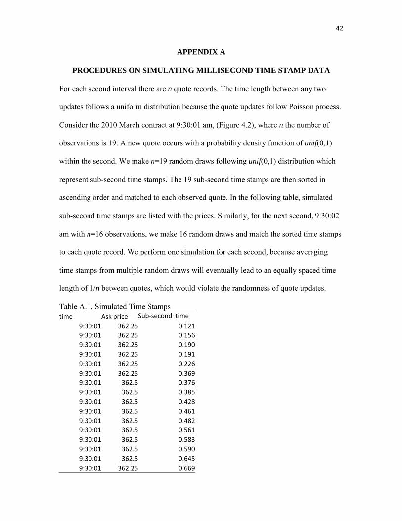
PROCEDURES ON SIMULATING MILLISECOND TIME STAMP DATA

For each second interval there are n quote records. The time length between any two

updates follows a uniform distribution because the quote updates follow Poisson process.

Consider the 2010 March contract at 9:30:01 am, (Figure 4.2), where n the number of

observations is 19. A new quote occurs with a probability density function of unif(0,1)

within the second. We make n=19 random draws following unif(0,1) distribution which

represent sub-second time stamps. The 19 sub-second time stamps are then sorted in

ascending order and matched to each observed quote. In the following table, simulated

sub-second time stamps are listed with the prices. Similarly, for the next second, 9:30:02

am with n=16 observations, we make 16 random draws and match the sorted time stamps

to each quote record. We perform one simulation for each second, because averaging

time stamps from multiple random draws will eventually lead to an equally spaced time

length of 1/n between quotes, which would violate the randomness of quote updates.

Table A.1. Simulated Time Stamps time  Ask price  Sub‐second  time 

9:30:01 362.25 0.121

9:30:01 362.25 0.156

9:30:01 362.25 0.190

9:30:01 362.25 0.191

9:30:01 362.25 0.226

9:30:01 362.25 0.369

9:30:01 362.5 0.376

9:30:01 362.5 0.385

9:30:01 362.5 0.428

9:30:01 362.5 0.461

9:30:01 362.5 0.482

9:30:01 362.5 0.561

9:30:01 362.5 0.583

9:30:01 362.5 0.590

9:30:01 362.5 0.645

9:30:01 362.25 0.669

43  

  

9:30:01 362.25 0.856

9:30:01 362.25 0.882

9:30:01 362.25 0.982

9:30:02 362.25 0.007

9:30:02 362.25 0.008

9:30:02 362.25 0.012

9:30:02 362.25 0.062

9:30:02 362.25 0.073

9:30:02 362.25 0.077

9:30:02 362.25 0.173

9:30:02 362.5 0.239

9:30:02 362.5 0.278

9:30:02 362.5 0.524

9:30:02 362.5 0.568

9:30:02 362.25 0.583

9:30:02 362.25 0.819

9:30:02 362.25 0.853

9:30:02 362.25 0.870

9:30:02 362.25 0.896

44  

  

APPENDIX B

PRICE DECOMPOSITION USING MODWT PROCEDURE

The Maximal Overlapping Discrete Wavelet Transformation (MODWT) (Percival and

Walden 2000) decomposes time series into add-up components which represent

variations at different time scales. As an illustration, figure B.1 plots a simulated random

walk price series for 30 seconds. The red bold lines are the average price for each non-

overlapping 5 seconds interval. This series can be decomposed into two parts—variations

within 5 seconds and at the 5 seconds time scale. For each 5-second interval, price

deviations R(n,t,s) = pi – S(n,t) represent the within 5-second variation component. The

average prices are the 5-second scale component, which can be further separated into

longer time scale variations like 10 or 20 seconds. However, this simple separation

method is not efficient because it fails to consider all possible time interval alignments,

e.g., a 5-second interval can be the 5th to 10th second as well as 7th to 12th second. As a

result, the extracted components are rough with jumps, e.g., the 5-second scale

component.

The MODWT procedure takes maximal overlapping wavelet transformation averages

at all possible time alignments. Because observations in price series are discrete, we use

the discrete Haar wavelet function as the signal filter. The Haar wavelet function is

defined as 1/ 0 0.51/ 0.5 0

, for a time scale s1. Notice that it is a zero-

mean filter symmetric over the time scale. It isolates the mean value of a series which

corresponds to extracting price deviations from the mean of each time scale. A set of

Haar filters covering time scales from s1 to sJ are defined as { ( ), (2 ),

45  

  

…, (2 )}. In practice, the set of filters are sequentially applied to extract variations

from the raw price series.

As an illustration, we apply the MODWT procedure on the price series of the 2010

nearby March contract. In figure B.2, we plot price variations at the 250 millisecond

(j=1), 32 second (j=8), 34.13 minute (j=14) time scales as well as post-filtered raw price

in the end. The high-low range of variations increase as scale expands from j=1 to 14.

The variance at 34.13 minutes is used as the benchmark measure of information driven

volatility. The filtered series are smooth, showing the efficiency of MODWT procedure.

Adding variations from each scale back to the filtered price recovers the original price

series in the lower panel of figure B.2.

46  

  

Figure B.1. Price Variations Within and at 5-second Time Scale

47  

  

Figure B.2. Application of the MODWT to the 2010 March Contract Bid Prices,

1/4/2010-1/29/2010

0 0.5 1 1.5 2 2.5

x 106

-1

0

1

250

ms

0 0.5 1 1.5 2 2.5

x 106

-1

0

1

32

s

0 0.5 1 1.5 2 2.5

x 106

-5

0

5

34.

13 m

in

0 0.5 1 1.5 2 2.5

x 106

380

400

420

Filt

ere

d P

rice

48  

  

Endnotes

                                                            1 A protective price band exists on the CME platform. In corn, the band is 20 ticks (5

cents/bu), meaning a specific market order cannot move price by more than 5 cents/bu.

2 ‘CFTC Moves to Rein In High-Speed Traders’, Wall Street Journal, August 22nd, 2013. 3 To account for an apparent reporting error, the January 2010 corn futures estimate was

adjusted, making it consistent with the aggregate agricultural futures markets and fourth

quarter 2010 corn estimates.

4 Notice in the long run, bid and ask quotes are assumed to follow the efficient price and

thus follow a random walk process.

5 Since May 2012, CME has changed corn trading hours several times (See Lehecka et al.

2014). We use the 9:45 am–1:00 pm window in the full sample for consistency.

6 Consider the December 2009 contract. To avoid maturity and overlapping data

problems, the data is September 1-November 30. Other contracts are treated similarly.

7 Tick size is selected for comparison because order execution price changes are often

viewed in this context, and because it is constant, making temporal comparisons easier.

8 These results are not presented but are available from the authors.

9 We also estimate the model including the first and last 15 minutes of data. As expected,

fundamental price variance represented by the 34.13 minute scale is higher because of

accumulated overnight information. As a result, estimated variance ratios are lower. For

the 2010 March contract, wavelet variance ratio at 250 millisecond scale drops from 2.27

to 2.18. The change suggests the excluded time exhibits higher fundamental volatility.