Arctic Sea Ice 2013: A Cooler Summer, but Still on Thin Ice Walt Meier, Code 615, NASA GSFC

Figure 2: Sea ice thickness estimates from March-April 2012 (left) and 2013 (right) from NASA Operation IceBridge flights. The scale is in meters.

Figure 1: Monthly average sea ice extent for September, the month of the minimum extent. The long term linear trend since 1979 is shown in blue, and the 1981-2010 average in red.

Figure 3: Ice age time series for March 1983-2013 (top) and ice age spatial distribution in March and September 2013 (bottom). Ice age provides a proxy for thickness (older ice is thicker ice). Colors denote age as given in the top figure with dark blue corresponding to open water or no data.

Trend = -13.7% per decade (relative to 1981-2010 avg.)

March 2013 Age September 2013 Age

March Sea Ice Fraction by Age Category

5

4

3

2

1

0 m

2013

Average 1981-2010

IceBridge images by N. Kurtz, NASA GSFC

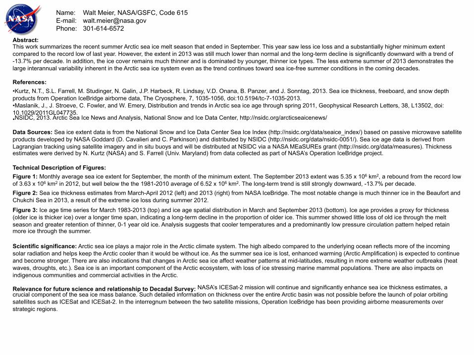
Abstract: This work summarizes the recent summer Arctic sea ice melt season that ended in September. This year saw less ice loss and a substantially higher minimum extent compared to the record low of last year. However, the extent in 2013 was still much lower than normal and the long-term decline is significantly downward with a trend of -13.7% per decade. In addition, the ice cover remains much thinner and is dominated by younger, thinner ice types. The less extreme summer of 2013 demonstrates the large interannual variability inherent in the Arctic sea ice system even as the trend continues toward sea ice-free summer conditions in the coming decades. References: • Kurtz, N.T., S.L. Farrell, M. Studinger, N. Galin, J.P. Harbeck, R. Lindsay, V.D. Onana, B. Panzer, and J. Sonntag, 2013. Sea ice thickness, freeboard, and snow depth products from Operation IceBridge airborne data, The Cryosphere, 7, 1035-1056, doi:10.5194/tc-7-1035-2013. • Maslanik, J., J. Stroeve, C. Fowler, and W. Emery, Distribution and trends in Arctic sea ice age through spring 2011, Geophysical Research Letters, 38, L13502, doi:10.1029/2011GL047735. • NSIDC, 2013. Arctic Sea Ice News and Analysis, National Snow and Ice Data Center, http://nsidc.org/arcticseaicenews/ Data Sources: Sea ice extent data is from the National Snow and Ice Data Center Sea Ice Index (http://nsidc.org/data/seaice_index/) based on passive microwave satellite products developed by NASA Goddard (D. Cavalieri and C. Parkinson) and distributed by NSIDC (http://nsidc.org/data/nsidc-0051/). Sea ice age data is derived from Lagrangian tracking using satellite imagery and in situ buoys and will be distributed at NSIDC via a NASA MEaSUREs grant (http://nsidc.org/data/measures). Thickness estimates were derived by N. Kurtz (NASA) and S. Farrell (Univ. Maryland) from data collected as part of NASA’s Operation IceBridge project. Technical Description of Figures: Figure 1: Monthly average sea ice extent for September, the month of the minimum extent. The September 2013 extent was 5.35 x 106 km2, a rebound from the record low of 3.63 x 106 km2 in 2012, but well below the the 1981-2010 average of 6.52 x 106 km2. The long-term trend is still strongly downward, -13.7% per decade. Figure 2: Sea ice thickness estimates from March-April 2012 (left) and 2013 (right) from NASA IceBridge. The most notable change is much thinner ice in the Beaufort and Chukchi Sea in 2013, a result of the extreme ice loss during summer 2012.

Figure 3: Ice age time series for March 1983-2013 (top) and ice age spatial distribution in March and September 2013 (bottom). Ice age provides a proxy for thickness (older ice is thicker ice) over a longer time span, indicating a long-term decline in the proportion of older ice. This summer showed little loss of old ice through the melt season and greater retention of thinner, 0-1 year old ice. Analysis suggests that cooler temperatures and a predominantly low pressure circulation pattern helped retain more ice through the summer. Scientific significance: Arctic sea ice plays a major role in the Arctic climate system. The high albedo compared to the underlying ocean reflects more of the incoming solar radiation and helps keep the Arctic cooler than it would be without ice. As the summer sea ice is lost, enhanced warming (Arctic Amplification) is expected to continue and become stronger. There are also indications that changes in Arctic sea ice affect weather patterns at mid-latitudes, resulting in more extreme weather outbreaks (heat waves, droughts, etc.). Sea ice is an important component of the Arctic ecosystem, with loss of ice stressing marine mammal populations. There are also impacts on indigenous communities and commercial activities in the Arctic. Relevance for future science and relationship to Decadal Survey: NASA’s ICESat-2 mission will continue and significantly enhance sea ice thickness estimates, a crucial component of the sea ice mass balance. Such detailed information on thickness over the entire Arctic basin was not possible before the launch of polar orbiting satellites such as ICESat and ICESat-2. In the interregnum between the two satellite missions, Operation IceBridge has been providing airborne measurements over strategic regions.

Name: Walt Meier, NASA/GSFC, Code 615 E-mail: walt.meier@nasa.gov Phone: 301-614-6572

Snow Science Results from Goddard’s Airborne Earth Science Microwave Imaging Radiometer (AESMIR)

Edward Kim, Code 617, Hemanshu Patel & Albert Wu--Emergent/Code 617, NASA GSFC

Figure 2: (above) Snow Water Equivalent (SWE) retrieved from AESMIR 10 & 18 GHz observations plus 36 GHz from AMSR-E. The patterns closely follow forest cover and elevation patterns in this part of Vermont.

Figure 3: (above, left) histograms of SWE derived from AESMIR (top) and from AMSR-E (bottom). Much larger AMSRE footprints have reduced sensitivity to both high & low end SWE values. The strong spike at zero SWE is largely a result of the AMSRE forest correction. (above, right) densest (red) areas in this forest density map correspond to many of the zero-SWE black areas in Fig 2.

Figure 1: AESMIR (circled in red above) on the NASA Wallops P-3 during 2009 flights.

Figure 4: (above) Image of AESMIR 10 GHz brightness temperature showing excellent sensitivity.

Burlington VT

island

RFI

lake

lake

Dense Forest

Pauses for Calibration

SWE

TB

Forest density

AMSRE SWE

AESMIR SWE

Sleepers River

Montpelier, VT

Name: Edward Kim, NASA/GSFC, Code 617 E-mail: ed.kim@nasa.gov Phone: 301-614-5653

Abstract: High resolution airborne snow water equivalent (SWE) retrievals from Goddard’s AESMIR passive microwave imager enable an evaluation of coarser-resolution satellite SWE accuracy in a forested area of Vermont. Satellite SWE underestimates vs. airborne SWE for both high and low SWE values. Effect is significantly attributed to forest cover, but imperfect match suggests other factors also contributing. There is room for an improved forest correction. High resolution SWE retrievals from sensors like AESMIR should lead to more accurate SWE estimates—both at a point and aggregated over watersheds. References: Kelly, R.E.J. (2009) The AMSR-E Snow Depth Algorithm: Description and Initial Results, Journal of The Remote Sensing Society of Japan. 29(1): 307-317. Data Sources: High res 10 & 18 GHz passive microwave data from AESMIR instrument (36 GHz channel was not flown). Satellite res 10, 18, & 36 GHz passive microwave data from AMSR-E instrument on Aqua. Aircraft Flight date 1/14/2009 from NASA Wallops. Snow-water equivalent calculated with Kelly (2009) algorithm. Ground truth from Sleepers River Research Watershed, Danville, VT measured 1/13/2009. Technical Description of Figures: Figure 1: AESMIR in flight on NASA Wallops P-3. AESMIR is installed in the bomb bay (circled in red in figure). Altitude 15500 ft for the flight lines depicted. Originally solely an engineering test flight, AESMIR worked well enough to extract science. Visually there was 100% snow cover in the area. Figure 2: Snow Water Equivalent (SWE) retrieved from AESMIR 10 & 18 GHz observations plus 36 GHz from AMSR-E. The patterns closely follow forest cover and elevation patterns in this part of Vermont. The box at Sleepers River shows where limited ground truth was collected the day before the flight. The diagonal box indicates an area of zero SWE due to the high forest density (red areas in Fig 3). Note that not all zero SWE (black) areas in Fig 2 correspond to high forest density (red) areas in Fig 3, so there are additional causes of zero retrieved SWE. Figure 3: On the left are histograms of SWE derived from AESMIR (top) and from AMSR-E (bottom). Comparing these shows that the much larger AMSR-E footprints have reduced sensitivity to both high & low end SWE values. The strong spike at zero SWE is largely a result of the AMSRE forest correction. On the right, densest (red) areas in this forest density map correspond to many of the zero-SWE black areas in Fig 2, but imperfect match suggests room for improved correction. High res AESMIR observations should lead to more accurate SWE estimates. Figure 4: This brightness temperature image for 10 GHz vertical polarization highlights excellent AESMIR’s sensitivity: mid-range values (yellow) corresponding to the widespread forest cover dominate although cooler green areas (towns, roads, ponds, and clearings) can be seen. Cold blue areas are Lake Champlain with shades of blue correspond to varying lake ice thickness and snow cover. Hot red areas are radio-frequency interference; cooler green areas are towns, roads, and clearings in forest cover Scientific significance: Although still a mainstay, passive microwave SWE retrievals have significant tlimitations including large footprint sizes from satellites (~25km) and masking due to forest cover. Some current SWE algorithms, such as the Kelly (2009) algorithm used here try to correct for this masking, but few studies have examined such a correction in detail. This study is an initial attempts to check the correction. Ground truth data (not shown) suggest both satellite and airborne SWE estimates are underestimating by a factor of 2-4. Relevance for future science and relationship to Decadal Survey: Any future snow mission concept must deal with masking by forests. The performance of potential techniques must be evaluated. High resolution airborne observations are a uniquely powerful tool for such evaluations.

0

50

100

150

200

250

300

350

400

2000 2001 2002 2003 2004 2005 2006 2007 2008

Dis

chag

e - c

ms

LU2003LU2010

Figure 1. a) Land Use map circa 2003 (Vietnam) and 1997 (Lao/Cambodia); b) newly developed Land Use map from 2010 MODIS data

Figure 3. Modeled discharge on the Sesan River using old (blue) and updated (yellow) Land Use products

Updating Land Cover and Soil Parameter Maps in the Lower Mekong River Basin

a) b)

Figure 2. Demonstrated feasibility of estimating Available Water Capacity map from modeled parameters

John D. Bolten, Code 617, NASA GSFC

Name: John D. Bolten, NASA/GSFC, Code 617 E-mail: john.bolten@nasa.gov Phone: 301-614-6529

Abstract: : ‘Project Mekong’ is a collaborative effort between NASA and the Mekong River Commission (MRC) aimed at improving flood and water management in the Lower Mekong. New floodplain management datasets and tools are being provided to MRC by integrating remotely sensed terrestrial water storage (GRACE), soil moisture (e.g., Advance Microwave Radiometer (AMSR) and future Soil Moisture Active Passive (SMAP)), and vegetation (Moderate Resolution Imaging Spectroradiometer (MODIS), Landsat) into the existing MRC Soil and Water Assessment tool (SWAT). An updated Land Use Land Cover map was developed using 2010 MODIS data and Landsat 30m multispectral data from 2004, 2009, and 2010 to derive a seamless mosaic for sub-region 6 (Figure 1). The mosaic was processed into a basic land cover map that included a water class, using methods from Ellis et al. (2011) and Spruce et al. (2013). These three LULC classes were then processed independently by converting the 30m class to the 240m scale, using a spatial averaging, fractional abundance estimation technique. The AWC map was estimated using the NASA Catchment Land Surface Model (CLSM) for years 2002-2010 over the Lower Mekong Basin (LMB) (Figure 2). References: Ellis, J.T., J.P. Spruce, R.A. Swann, J.C. Smoot, and K.W. Hilbert, 2011: An assessment of coastal land use and land cover change from 1974-2008 in the vicinity of Mobile Bay, Alabama, Journal of Coastal Conservation, 15:139-149. Spruce, J.P., J.C. Smoot, J.T., Ellis, K. Hilbert, and R. Swann, 2013: Geospatial method for computing supplemental multi-decadal U.S. coastal land-use and land-cover classification products, using Landsat data and C-CAP products. Geocarto International, published on-line, DOI:10.1080/10106049.2013.798357. Data Sources: MODIS MCD12C1 land cover classification data obtained from the NASA Land Processes Distributed Active Archive Center (2010), MODIS MCD12C1 (Collection 5). USGS/Earth Resources Observations and Science (EROS), Sioux Falls, South Dakota; Landsat TM winter data from 2004, 2009, and 2010 obtained from the NASA Land Processes Distributed Active Archive Center, USGS/Earth Resources Observations and Science (EROS), Sioux Falls, South Dakota. Technical Description of Figures: Figure 1: . a) Land Use map circa 2003 (Vietnam) and 1997 (Laos/Cambodia); b) newly developed Land Use map from 2010 MODIS data. The updated map shows significant changes in cultivated lands in Vietnam and Cambodia. Figure 2: Demonstrated feasibility of estimating Available Water Capacity map from modeled parameters. Figure 3: Results of analysis provided by MRC Stakeholders – The modeled discharge from the SWAT model on the Sesan River using old (blue) and updated (yellow) Land Use products. Scientific significance: Changes in Land Use and soil parameter maps are envisioned to have significant effects in surface runoff and water storage within the soil profile. Such changes will have a notable impact on MRC SWAT discharge estimates and resulting decisions regarding floodplain management. Therefore, the updated maps, which are constrained by observed dynamics in water and vegetation, are envisaged to provide more realistic estimates of runoff and enhanced floodplain management from its application. Relevance for future science and relationship to Decadal Survey: In preparation for the upcoming Decadal Survey mission, Soil Moisture Active Passive (SMAP), it is essential that we investigate new methods of applying and validating the utility of remotely-sensed soil moisture.