
Archiving Scienti c Data - University of Edinburgh
50
Archiving Scientific Data PETER BUNEMAN University of Edinburgh SANJEEV KHANNA University of Pennsylvania KEISHI TAJIMA Japan Advanced Institute of Science and Technology and WANG-CHIEW TAN University of California, Santa Cruz Archiving is important for scientific data, where it is necessary to record all past versions of a database in order to verify findings based upon a specific version. Much scientific data is held in a hierachical format and has a key structure that provides a canonical identification for each element of the hierarchy. In this paper we exploit these properties to devlop an archiving technique that is both efficient in its use of space and preserves the continuity of elements through versions of the database, something that is not provided by traditional minimum-edit-distance diff approaches. The approach also uses timestamps. All versions of the data are merged into one hierarchy where an element appearing in multiple versions is stored only once along with a timestamp. By identifying the semantic continuity of elements and merging them into one data structure, our technique is capable of providing meaningful change descriptions, the archive allows us to easily answer certain temporal queries such as retrieval of any specific version from the archive and finding the history of an element. This is in contrast with approaches that store a sequence of deltas where such operations may require undoing a large number of changes or significant reasoning with the deltas. A suite of experiments also demonstrates that our archive does not incur any significant space overhead when contrasted with diff approaches. Another useful property of our approach is that we use XML format to represent hierarchical data and the resulting archive is also in XML. Hence, XML tools can be directly applied on our archive. In particular, we apply an XML compressor on our archive, and our experiments show that our compressed archive outperforms compressed diff-based repositories in space efficiency. We also show how we can extend our archiving tool to an external memory archiver for higher scalability and describe various index structures that can further improve the efficiency of some temporal queries on our archive. Categories and Subject Descriptors: H.2.8 [Database Management]: Scientific Databases; H.3.7 [Information Storage and Retrieval]: Collection, Dissemination, Systems issues; H.2.1 [Database Management]: Data models General Terms: Algorithms, Design, Experimentatal Analysis, Management Additional Key Words and Phrases: Keys for XML Authors’ addresses: Peter Buneman, Email: [email protected]; Sanjeev Khanna, Email: [email protected]; Keishi Tajima, Email: [email protected]; Wang-Chiew Tan, Email: [email protected]. Permission to make digital/hard copy of all or part of this material without fee for personal or classroom use provided that the copies are not made or distributed for profit or commercial advantage, the ACM copyright/server notice, the title of the publication, and its date appear, and notice is given that copying is by permission of the ACM, Inc. To copy otherwise, to republish, to post on servers, or to redistribute to lists requires prior specific permission and/or a fee. c 20 ACM 0362-5915/20/0300-0001 $5.00 ACM Transactions on Database Systems, Vol. , No. , 20, Pages 1–39.
Transcript of Archiving Scienti c Data - University of Edinburgh

Archiving Scientific Data
PETER BUNEMAN
University of Edinburgh
SANJEEV KHANNA
University of Pennsylvania
KEISHI TAJIMA
Japan Advanced Institute of Science and Technology
and
WANG-CHIEW TAN
University of California, Santa Cruz
Archiving is important for scientific data, where it is necessary to record all past versions of adatabase in order to verify findings based upon a specific version. Much scientific data is held in ahierachical format and has a key structure that provides a canonical identification for each elementof the hierarchy. In this paper we exploit these properties to devlop an archiving technique that is
both efficient in its use of space and preserves the continuity of elements through versions of thedatabase, something that is not provided by traditional minimum-edit-distance diff approaches.The approach also uses timestamps. All versions of the data are merged into one hierarchywhere an element appearing in multiple versions is stored only once along with a timestamp.By identifying the semantic continuity of elements and merging them into one data structure,our technique is capable of providing meaningful change descriptions, the archive allows us toeasily answer certain temporal queries such as retrieval of any specific version from the archiveand finding the history of an element. This is in contrast with approaches that store a sequenceof deltas where such operations may require undoing a large number of changes or significantreasoning with the deltas.
A suite of experiments also demonstrates that our archive does not incur any significant spaceoverhead when contrasted with diff approaches. Another useful property of our approach is thatwe use XML format to represent hierarchical data and the resulting archive is also in XML. Hence,XML tools can be directly applied on our archive. In particular, we apply an XML compressoron our archive, and our experiments show that our compressed archive outperforms compresseddiff-based repositories in space efficiency. We also show how we can extend our archiving tool toan external memory archiver for higher scalability and describe various index structures that canfurther improve the efficiency of some temporal queries on our archive.
Categories and Subject Descriptors: H.2.8 [Database Management]: Scientific Databases;H.3.7 [Information Storage and Retrieval]: Collection, Dissemination, Systems issues; H.2.1[Database Management]: Data models
General Terms: Algorithms, Design, Experimentatal Analysis, Management
Additional Key Words and Phrases: Keys for XML
Authors’ addresses: Peter Buneman, Email: [email protected]; Sanjeev Khanna, Email:[email protected]; Keishi Tajima, Email: [email protected]; Wang-Chiew Tan, Email:[email protected] to make digital/hard copy of all or part of this material without fee for personalor classroom use provided that the copies are not made or distributed for profit or commercialadvantage, the ACM copyright/server notice, the title of the publication, and its date appear, andnotice is given that copying is by permission of the ACM, Inc. To copy otherwise, to republish,to post on servers, or to redistribute to lists requires prior specific permission and/or a fee.c© 20 ACM 0362-5915/20/0300-0001 $5.00
ACM Transactions on Database Systems, Vol. , No. , 20, Pages 1–39.

2 · Buneman, Khanna, Tajima, and Tan
1. INTRODUCTION
Scientific databases are published on the Web to disseminate the latest research.As new results are obtained these databases will be updated, mainly by adding data,but also by modifying and deleting existing data. Since other research may be basedon a specific version of a database, it is important to create archives containing allprevious states of the data. Failure to do so means that scientific evidence maybe lost and the basis of findings cannot be verified. A search of scientific dataavailable on the Web [CELLBIODBS ] suggests that archiving is an ubiquitousproblem. Even databases of physical constants [PHYSICSCONSTANTS ] are less“constant” than one might naively imagine. The onus of keeping archives typicallyfalls on the producers of data, but there are no general techniques for efficientlykeeping long-term archives that also provide efficient support for basic operationssuch as retrieval of a past version from the archive and tracing the evolutionaryhistory of an element in the archive.
As an example of the issues involved, consider two widely used datasets in geneticresearch: Swiss-Prot [Bairoch and Apweiler 2000], a protein sequence database,and On-line Mendelian Inheritance in Man (OMIM) [OMIM 2000], a database ofdescriptions of human genes and genetic disorders. Both databases have a similarhierarchical structure and both are heavily curated, i.e., they are maintained withextensive manual input from experts in the field. In the case of Swiss-Prot, a newversion is produced approximately every four months, and all old versions are kept.On the other hand, in the case of OMIM, a new version is produced almost everyday, but only occasionally is a (printed) archive produced. Swiss-Prot and OMIMare two contrasting examples of archiving practices1. There is an obvious trade-off between the frequency with which the database is “published” and the spacerequired for complete archiving. Although keeping all old versions allows one toquickly obtain an old version, such an archiving method clearly does not scale wellin the long run or if the database is published very frequently, such as like OMIM.Even if the issue of space is not critical, and we choose to keep all versions, thereis also the issue of the efficiency with which one can query the temporal historyof some part of the database. For example, to find when a given observation firstappeared in history or when it was last changed may require one to locate thatobservation in each of a very large number of versions.
Another approach to archiving is to keep a record of the changes – a “delta”– between every pair of consecutive versions. We will call this the sequence-of-
delta approach throughout the paper. Such a method of archiving clearly conservesspace and scales well. In this approach, however, retrieving an old version mightinvolve undoing or applying many deltas. Likewise, the efficiency of finding theevolutionary history of an element is also a problem and may require significant
1It should be mentioned that, in addition to the published versions, both SWISS-PROT andOMIM keep audit trails of the edits to the data, so there is more historical information than isapparent from the archives. However it is not clear that either organization could easily producethe state of its data as it was at some arbitrary past time.
ACM Transactions on Database Systems, Vol. , No. , 20.

Archiving Scientific Data · 3
Version 1 Version 2 Output of diff
<gene>
<id>6230</id>
<name>GRTM</name>
<seq>GTCG...</seq>
<pos>11A52</pos>
</gene>
<gene>
<id>2953</id>
<name>ACV2</name>
<seq>AGTT...</seq>
<pos>08A96</pos>
</gene>
<gene>
<id>2953</id>
<name>ACV2</name>
<seq>GTCG...</seq>
<pos>11A52</pos>
</gene>
<gene>
<id>6230</id>
<name>GRTM</name>
<seq>AGTT...</seq>
<pos>08A96</pos>
</gene>
2,3c
<id>2953</id>
<name>ACV2</name>
8,9c
<id>6230</id>
<name>GRTM</name>
Fig. 1. Two versions and the diff.
reasoning with the deltas.Tools for keeping changes made to text documents, such as CVS [CVS ] of-
ten adopt the sequence-of-delta approach. Such tools typically use line-diff algo-rithms [Miller and Myers 1985; Myers 1986] to describe changes. Tree diffs havealso been developed for XML and other hierarchical structures [Zhang and Shasha1989; Chawathe et al. 1996; Chawathe and Garcia-Molina 1997; Cobena et al. 2001].These diff algorithms compute deltas that are also based on the notion of minimal-edit-distance, and we shall refer to these as diff-based aproaches . Measuring the”diff” of two structures is one of a number of ways of computing a delta, otherscould be based, for example, on edit scripts or transaction logs. The problem withthe diff-based approach is that it may ignore the semantic continuity of data ele-ments. As an example, suppose we have a database containing data of two genes,as shown in Version 1 of Figure 1. It was later discovered that the information onone gene had been confused with the other, and the data was corrected as shownin Version 2. A diff algorithm might explain the change as genes changing theirnames and id numbers, as shown by the diff output in Figure 1; It says that lines 2-3of Version 1 should be replaced with <id>2953</id><name>ACV2</name>, i.e., thegene GRTM changed its id to 2953, and also changed its name to ACV2. Similarly,the diff says the gene ACV2 changed its id to 6230, and also changed its name toGRTM.
If we are only interested in retrieving an entire (past) version from a diff-basedrepository, such nonsensical change descriptions do not surface. However, if weare interested in finding the temporal history of an element in the database, thediff-based approach may require one to perform some complicated analysis on thediff scripts. This example suggests that there is a temporal invariance of keys thatshould be captured by an archiving system. We would like an archiving systemthat is able to preserve the continuity of data elements through time.
The archiving techniques described in this paper stem from the requirementsand properties of scientific databases. They are, of course, applicable to data inother domains, but they are especially appropriate to scientific data for a variety ofreasons. First, as we have noted, archiving is important for scientific data. Second,
ACM Transactions on Database Systems, Vol. , No. , 20.
4 · Buneman, Khanna, Tajima, and Tan
scientific data is largely accretive or ”write mostly”, and the transaction rate is low.In particular, an individual data entry will be modified infrequently. Third, muchscientific data is kept in well-organized hierarchical data formats and is naturallyconverted into XML. Finally, this hierarchically structured data usually has a key
structure which is explicit in the design of the format. The key structure providesa canonical identification for every part of the document, and it is this structurethat is the basis for our techniques.
Our archiver leverages these properties and effectively stores multiple versionsof hierarchical data in a compact archive that can easily support certain temporalqueries by using the following techniques:
—Identifying changes based on keys. In contrast to the many existing toolsthat use the diff-based approach based on minimum edit distance, we identify thecorrespondence and changes between two given versions based on keys. We willcall this approach key-based approach. By this, our archive can preserve semanticcontinuity of each data element in the archive, and can efficiently support querieson the history of those elements.
—Merging versions based on keys. In contrast to the delta-based approach,we merge all versions into one hierarchy. We will call this approach merging
approach. An element may appear in many versions, but we identify those occur-rences using the key structure and store it only once in the merged hierarchy. Thesequence of versions in which an element appears is described by its timestamp
(a sequence of version numbers) and is stored together with that element. Sincechanges to our database are largely accretive and an element is likely to exist fora long time, we can compactly represent its timestamp using time intervals ratherthan a sequence of version numbers. Notice that the description of changes isgrouped by elements in this structure while the description of changes is groupedby time in the sequence-of-delta approach. When compared with the latter ap-proach, the former can easily support both the retrieval of very old versions orqueries on the history of an element.
—Inheritance of timestamps. Conceptually, a timestamp is stored with everyelement to indicate its existence at various points in history. In actual implemen-tation, a timestamp is stored at a child element only when it is different fromthe timestamp of its parent element. Since most changes are insertions of newelements, it is likely that an element in the archive has identical timestamp toits parent element. Hence a fair amount of space overhead is usually avoided byinheriting timestamps.
There are two orthogonal choices to be made among the possible descigns of anarchiver: whether to use a diff-based or key-based method of describing change andwhether to use a sequence-of-delta or a merging technique in recording the change.Our approach is key-based + merging approach while systems such as CVS usea diff-based + sequence-of-delta approach. The other two combinations are alsopossible, and in fact, we also use diff-based + merging approach for unkeyed partof the data. The details are explained later.
Another interesting aspect of our approach is that our archive can be easily rep-resented as yet another XML document. Our choice of using XML is motivated in
ACM Transactions on Database Systems, Vol. , No. , 20.
Archiving Scientific Data · 5
db
dept
name
finance fn
John Doe
ln
emp
123−4567
telsal
95K
db
dept
telfn ln
emp
tel
dept
name
finance
db
dept
fn
emp
John
ln
Doe 123−4567
tel
90K
sal
name
marketing fn
emp
John
ln
Doe
name
finance fn ln
SmithJane
emp
db
dept
name
finance
sal
95KJane Smith 123−6789 112−3456
PSfrag replacements
Version 1 Version 2 Version 3
Version 4
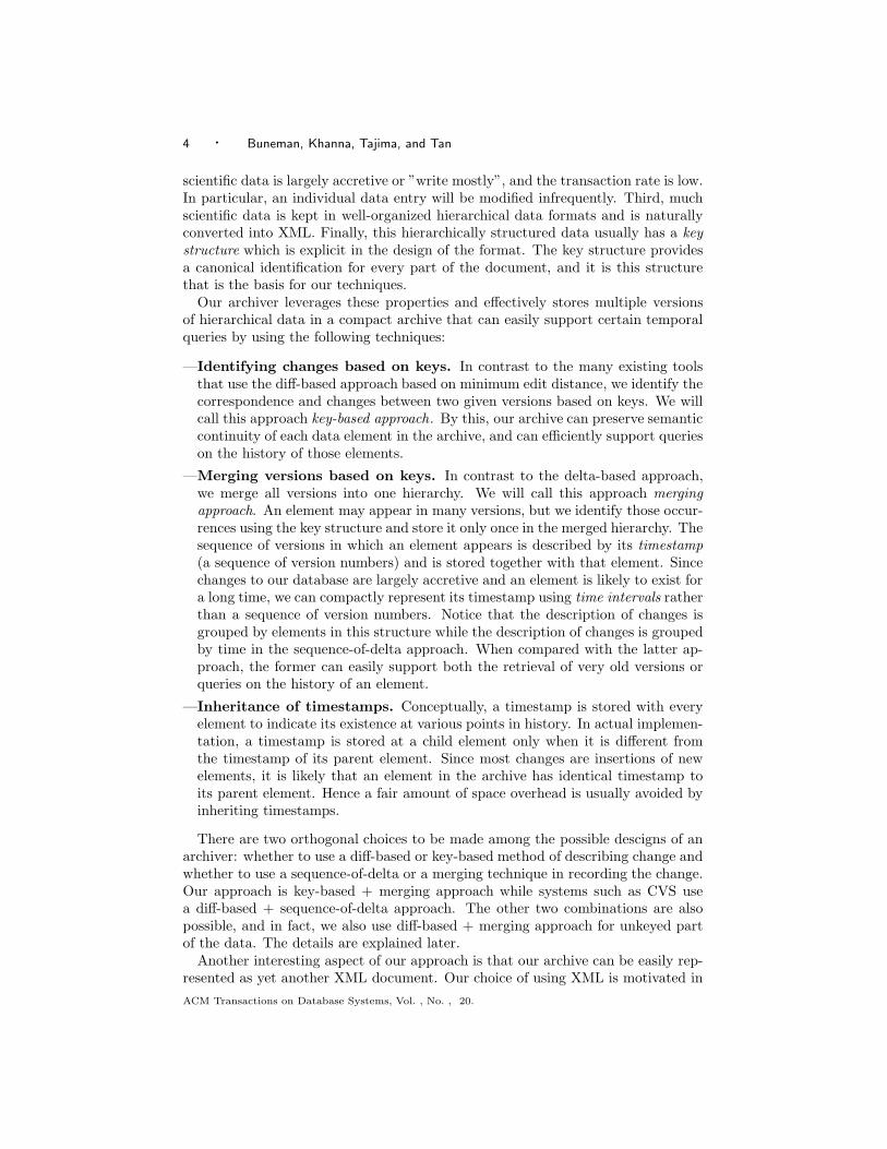
Fig. 2. A sequence of versions
part by the existence of many biological databases in hierarchical formats, whichare close to the XML data model. Many of these databases are also moving to-wards support for XML (e.g., Swiss-Prot [EMBL-EBI (European BioinformationsInstitute) ]). Since XML is also a widespread format for representation and ex-change, we assume sources are provided in XML and chose to represent our archivein XML. Our choice of XML also allows us to leverage many existing XML toolssuch as XML editors, parsers, etc. that are readily available. In particular, we sub-sequently use an XML compressor such as XMill [Liefke and Suciu 2000] to furthercompress the archive (see Section 5).
This paper describes the archiving technique in detail and gives some experi-mental data on its performance. The technique is an extension of the “persistentdata structures” of Driscoll et al. [Driscoll et al. 1989] (see Section 8). In order toestablish the viability of this approach, we do several things:
—We show that the compacted archive can be constructed efficiently, i.e., a newversion can be efficiently merged with an existing archive.
—We show, experimentally, that the space overhead for our compacted archive iscomparable to the existing approaches.
—We also establish experimentally that our compacted archives work well withXMill, and outperform compressed diff-based repositories in terms of space effi-ciency.
—Since our archive preserves the semantic continuity of elements, it is easy tosupport various temporal queries more efficiently than delta-based approaches.We also show that we can further improve the efficiency of answering certain
ACM Transactions on Database Systems, Vol. , No. , 20.

6 · Buneman, Khanna, Tajima, and Tan
name
finance fn lnfn
John Doe
ln
123−4567
tel{123−4567} tel{112−3456}
112−3456
sal
95KJane Smith
sal
95K
emp{fn=John,ln=Doe} emp{fn=Jane,ln=Smith}
123−6789
tel{123−6789}
dept{name=finance}
db
Fig. 3. Version 4 annotated with key values.
queries by defining simple index structures on top of our archive.
For example, on the basis of our experimental findings for OMIM, which is notadequately archived (we recorded 100 versions over roughly 100 days), we predictthat we should be able to construct a compacted archive for a year in less than1.12 times the space of the last version. Moreover, the archive, under XMill, willcompress to 40% of the size of the last version.
2. AN EXAMPLE
A simple example illustrates how the archiver works. In Figure 2, we see a sequenceof versions of a company database containing information about its employees ineach department. Every department can be identified by its department name, i.e.,name is the key for departments. Within each department, every employee can beuniquely identified by the employee’s firstname and lastname, i.e., firstname andlastname is the key for employees. Notice that it is possible for two employees havethe same firstname and lastname if they belong to distinct departments (e.g., JohnDoes of version 3). Each employee also has at most one salary value, and one ormore telephone numbers. Figure 3 shows version 4 of Figure 2 with key informationannotated on nodes. For example, emp nodes are annotated with firstname andlastname values and tel nodes are annotated with its subvalue.
Figure 4 shows how those versions can be merged into one compact archive by“pushing down” timestamps. We first start at the top level of the versions, anddetermine the nodes that correspond to one another across all versions accordingto their key values. At the top level, each version has only one root node andthey correspond to one another. We merge corresponding nodes together, annotatethe resulting node with the version numbers of all merged nodes and push thetimestamp of each merged node down their respective subtrees. We recursivelyinvoke this procedure for the children of merged nodes until we reach the leaves.The root node in the archive is used to keep track of the possibility that an archivedversion is empty. For example, suppose the database is empty at version 5. If version5 is archived, then the node root will have timestamp t=[1-5] while the node db willhave timestamp t=[1-4], indicating that version 5 is an empty database2.
2Note that the current version number is the largest number in the root node. Instead of using aroot node, one can also choose to keep track of the next version number as meta-information andincrement the next version number whenever a version is archived.
ACM Transactions on Database Systems, Vol. , No. , 20.

Archiving Scientific Data · 7
name
finance fn
John Doe
ln
123−4567
tel{123−4567}sal
95K
t=3 t=4
dept{name=finance}
123−6789
fn ln
Smith 95K
sal, t=[4]
Jane
tel{123−6789}, t=[4]
root, t=[1−4]
db
emp{fn=John,ln=Doe}, t=[3−4]
90K
dept{name=marketing}, t=[3]
112−3456
tel{112−3456}, t=[4]
emp{fn=Jane,ln=Smith}, t=[2,4]
Fig. 4. “Pushing” time down. Example of an archive.
Observe that in the resulting archive in Figure 4, nodes appearing in many ver-sions are stored only once in the archive. If a node occurs in version i, then thetimestamp of the corresponding node in the archive contain i. We use time inter-vals to describe the sequence of versions for which a node exists. For example, thetime intervals [1-3,5,7-9] denotes the set {1,2,3,5,7,8,9}. If a node does not have atimestamp, it is assumed to inherit the timestamp of its parent. For example, thefinance dept node inherits the timestamp t=[1-4] from its parent db node. Observealso that it is a property of the archive that the timestamp of a node is always asuperset of timestamps of any descendant node. This archive can be representedin XML, as shown in Figure 5. For example, employee John Doe of the financedepartment has a timestamp <T t="3-4"> around it, indicating that the entiresubtree within exists in versions 3 and 4. Furthermore, during these times, Johnhas salary 90K at version 3 and 95K at version 4.
We may assume that the tag T is in a separate namespace [W3C 1999a]. It isalso easy to see that to reconstruct any previous version, all we need is a simplescan through the “compacted” document. Notice that information on changes isgrouped by elements in this structure while information on changes is grouped bytime in the sequence-of-delta approach. Also, our archive ignores the order amongelements with keys. If the emp node corresponding to John Doe occurs in version5 after the emp node corresponding to Jane Smith, it might still be represented inthe archive before Jane Smith.
There are two immediate caveats about this approach. First, what happens ifthe data does not have a key system, i.e., there are nodes that cannot be uniquelyidentified by their paths and any subelements? We have found that most scientificdata sources have a well-organized key system. However, there are cases in whichwe cannot define appropriate keys for all the nodes down to the leaves. For example,some data may be free text represented as a sequence of <line> elements and some<line> elements may have same text value. Even in such a case, provided the uppernodes in the tree have keys, we can still “push down” the timestamps in the upperpart, stop merging, and apply a conventional diff algorithm when we reach elementswithout keys, such as <line> elements in the example above. In fact, if the entiredocument does not have appropriate keys, our archiving technique is very close tothe SCCS approach [Rochkind 1975] (see also Section 8). The second caveat is
ACM Transactions on Database Systems, Vol. , No. , 20.

8 · Buneman, Khanna, Tajima, and Tan
<T t="1-4">
<root>
<db>
<T t="3">
<dept>
<name>marketing</name>
<emp>
<fn>John</fn> <ln>Doe</fn>
</emp>
</dept>
</T>
<dept>
<name>finance</name>
<T t="3-4">
<emp>
<fn>John</fn> <ln>Doe</ln>
<T t="3"><sal>90K</sal></T>
<T t="4"><sal>95K</sal></T>
<tel>123-4567</tel>
</emp>
</T>
<T t="2,4">
<emp>
<fn>Jane</fn> <ln>Smith</ln>
<T t="4"><sal>90K</sal></T>
<T t="4"><tel>123-4567</tel></T>
<T t="4"><tel>112-3456</tel></T>
</emp>
</T>
</dept>
</db>
</root>
</T>
Fig. 5. XML representation of the archive in Figure 4.
whether the new structure really is smaller than the accumulated past versions.Here, we capitalize on the fact that the timestamps associated with elements canbe compactly represented as a small number of intervals and are often inheritedfrom a parent element. Our experiments in Section 5 validate this.
In the following sections we first explain the notion of keys for hierarchical datathat plays an important role in our archiving system. Next, we describe the mainmodules of the archiver in detail, including key annotation, nested merge and fin-gerprinting of keys for efficiency. We then show some experimental results on somewidely used biological data sets and also on some synthetic data. The followingsections show how the whole process can be implemented on large data sets usingexternal memory and show how versions and the temporal history of an elementmay be efficiently retrieved.
ACM Transactions on Database Systems, Vol. , No. , 20.

Archiving Scientific Data · 9
3. KEYS FOR HIERARCHICAL DATA
The general notion of a key for XML is described in [Buneman et al. 2001] and sum-marized in Appendix A. Informally, a key is an assertion of the form (Q, {P1, . . . , Pk})where Q, P1, . . . , Pk are all path expressions in a syntax like XPath [W3C 1999b]but consisting only of node and attribute names. The path Q identifies the target
set for the key – the set of nodes to be constrained by the key. The paths P1, . . . , Pk
are the key paths and are analogous to the key attributes in the relational setting.An XML document satisfies a key (Q, {P1, . . . , Pk}) if
—from any node identified by Q, every path Pi (1 ≤ i ≤ k) exists uniquely, and
—if two nodes n1 and n2 identified by Q have the same value at the end of eachkey path in {P1, . . . , Pk}, then n1 and n2 are identical nodes.
Example: (/book, {isbn}). Every book child of the root must have a unique isbnchild, and if two such book nodes have the same value for their isbn children, thenthey are the same node.
In the definition above, the path Q in a key starts at the root. We shall need tobe able to define keys starting from one of a set of “context nodes”. For examplewe would like to say that beneath any book node, a chapter node is specified byits chapter-number child. But this is to hold only beneath some book node – notglobally. We can specify such a key simply by adding to the definition the contextpath, in this case (/book, (chapter, {chapter-number})). Such a key is called arelative key. All the keys we deal with will be relative.
As a further example, version of the company database satisfies the following keyconstraints.
—(/, (db, {})). There is at most one db element below the root.
—(/db, (dept, {name})). Every dept node within a db node can be uniquely iden-tified by the contents of its name subelement.
—(/db/dept, (emp, {fn, ln})). Every emp node within a dept node along the path/db/dept can be uniquely identified by the contents of its fn and ln subelements.
—(/db/dept/emp, (sal, {})). There is at most one sal subelement under each empnode along the path /db/dept/emp.
—(/db/dept/emp, (tel, {.})). Every tel node within an emp node along the path/db/dept/emp can be uniquely identified by its contents (“.” denotes the emptypath). That is, the same telephone number cannot be repeated below an empnode.
The keys shown above are rather simple. For the scientific data that we use forour experiments, keys are also simple. (See Appendix B.) Observe that for strongkeys, whenever a key (Q, (Q′, {P1, ..., Pk})) exists, the keys (Q/Q′, (Pi, {})),1 ≤ i ≤ k are implied (Pi is a non-empty key path). Although we do not explicitlystate these keys, we shall always assume that they are part of the key specification.We remark that for documents that are standard and consistent representations ofrelations in XML, the set of keys can be automatically generated from the relationalschema.Some terminology. We say a node or an element is keyed if it has a key. In otherwords the sequence of tag names from the root to this node is equal to the concate-
ACM Transactions on Database Systems, Vol. , No. , 20.

10 · Buneman, Khanna, Tajima, and Tan
nation of context and target path of some key. In the example databases in Figure 2,every non-leaf node is keyed. Given a set of keys, we consider the paths given bythe concatenation of context and target paths for every key in the key specification.We say a path in this set is a frontier path if it is not a proper prefix of some otherpath in the set. A node is a frontier node if the sequence of tag names from rootto that node equals to some frontier path. In other words, a frontier node is thedeepest possible keyed node. For example, the key specification for the companydatabase has frontier paths /db/dept/name, /db/dept/emp/fn, /db/dept/emp/ln,/db/dept/emp/sal, and /db/dept/emp/tel. An example of a frontier node is name,but the node emp is not a frontier node. Obviously, there can be unkeyed nodesbeyond frontier nodes. If there are area code and number subelements within eachtel node, then these subelements are unkeyed nodes beyond the frontier node tel.
Assumptions about the key structure. In this paper, we assume the given keyspecification possess the following properties.
—We assume that every key defined for a node is relative to its parent node andkeys are defined up to a certain depth in the tree. For example, to identify anemp node that lies on the path /db/dept/emp requires one to first identify thecorrect db and dept nodes. That is, the key defined for an emp node is relative toits parent node, dept, and the key defined for a dept node is relative to its parentnode, db. Such keys are called “insertion-friendly” keys in [Buneman et al. 2001].
—Given a set of keys that a document satisfies, every node that does not occurbeneath frontier nodes is keyed. In other words, we assume that the keys “cover”every node that does not occur beneath frontier nodes. For example, there cannotbe some unkeyed node directly under emp since emp nodes are not frontier nodes.
—Our last restriction is that nodes that exist beneath some key path cannot bekeyed. Given a key (Q2, (Q
′
2, {...})), there cannot be a key (Q1, (Q′
1, {P1, ..., Pk}))where k ≥ 1 such that Q1/Q′
1/Pi is a proper prefix of Q2/Q′
2, for some i ∈ [1, k].The reason is that the order among keyed nodes is unimportant and since theorder among element nodes in an XML value is important for (key) value equality,the nodes beneath Q1/Q′
1/Pi for every i ∈ [1, k] should not be keyed. Otherwise,the key of a node in Q1/Q′
1 may be different each time the order among keyednodes beneath Q1/Q′
1/Pi changes.
The first assumption makes it easy for us to determine the correspondences betweennodes in the archive and a version as we go down the trees starting from the root.Although this assumption may seem restrictive, we have found that the keys forour experimental data naturally adhere to this assumption. The second assumptionis a restriction made only to simplify the discussion of our merge algorithm inSection 4.2. In the event that non-keyed nodes above frontier nodes exist, ourarchiver handles these nodes by applying conventional diff techniques on the nodes,since no key information is known about these nodes. The last assumption is infact not required due to the “top-down” localized merging of nodes in our mergealgorithm as discussed in Section 4.2. Two nodes in Q1/Q′
1 are merged only whentheir corresponding values at Q1/Q′
1/Pi are equal. In case the two nodes at Q1/Q′
1
are merged, the two corresponding nodes at Q2/Q′
2 are also merged by virtue thatthey occur in a key path of Q1/Q′
1.
ACM Transactions on Database Systems, Vol. , No. , 20.

Archiving Scientific Data · 11
New version
Keys
ArchiveAnnotate Keys,Timestamps
Annotate Keys
Nested Merge New Archive
Fig. 6. Main modules in our archiving system.
4. MAIN MODULES
We now describe our main modules: Annotate Keys and Nested Merge as shown inFigure 6. The module Annotate Keys annotates each keyed element in a documentor an archive with its key value. For example, Annotate Keys will transform theversion 4 of the database in Figure 2 into the database shown in Figure 3. Thekey values allow Nested Merge to determine immediately the corresponding nodesin the archive and version. A node in the archive corresponds to a node in theversion if they have the same key value. The module Nested Merge merges a newversion into the existing archive according to correspondence of nodes between thearchive and version. When annotating archives, we also need some processing ofthe timestamps, which will be explained later.
4.1 Annotate Keys
In this section, we show how, given a key specification, one can annotate everykeyed node in an XML document with its key value. For example, emp nodes inthe version of Figure 3 and the archive of Figure 4 are annotated with these keys —emp{fn=Jane, ln=Smith} and emp{fn=John, ln=Doe}. The resulting tree is suchthat every keyed node can be identified by the path from root to that node bytaking into account existing key values as well.
The idea behind the algorithm Annotate Keys is to scan through the document,looking out for nodes that should be keyed and nodes that contain key path values.Given a key (Q, (Q′, {P1, ..., Pk})), a node that is on the path Q/Q′ is a node tobe keyed and a node that is on the path Q/Q′/Pi, where i ∈ [1, k], is a node thatcontains a key path value. (The key path value is the XML value rooted under thatnode.) As an XML document is scanned in document order, an open tag is alwaysencountered before the corresponding close tag (assuming that the document iswell-formed). Alternatively, we say a node is entered first before it is exited in thetree representation of the XML document. Observe that by the time one exits anode n that needs to be keyed (i.e., n is along the path Q/Q′), the nodes containingkey path values of n would already have been visited (i.e., those nodes are alongpaths Q/Q′/Pi, i ∈ [1, k]).
Whenever we encounter a node that contains a key path value, we memorizethe entire “subtree” of the node and store the subtree value at the node. One canavoid storing large key path values by computing and storing its fingerprint instead.We describe how one can compute fingerprints in Section 4.3. We emphasize thatfingerprints are used entirely for efficiency purposes. A fingerprint uses less space
ACM Transactions on Database Systems, Vol. , No. , 20.

12 · Buneman, Khanna, Tajima, and Tan
than the actual value and it is faster to compare two fingerprints (comparisonsare done in Nested Merge described in Section 4.2) of the respective key valuesinstead of comparing the actual key values. In fact, most well-organized databaseshave small key path values and hence, fingerprints might not be necessary for suchdatabases.
The algorithm below describes how to annotate keyed nodes of an incomingversion with its key value. We assume that the document D satisfies the keyconstraints imposed by K which consists of q keys (C1, (S1, {P11, ..., P1m1
})),...,(Cq , (Sq , {Pq1, ..., Pqmq
})). We let CSi denote the sequence of label names in Ci
followed by Si of the ith key and let p(M) denote the sequence of label names ona stack M . The process of annotating keyed nodes in D can occur during the timethe document is first read into memory.Algorithm Annotate Keys(D, K)
1. Initialize an empty main stack M .2. Traverse the nodes of tree D in document order (preorder).
(a) Upon entering a node, push the node label onto all active stacks.If p(M) = CSi for some i, then
initialize an empty stack Mij for each key path, Pij , j ∈ [1, mi].For each stack Mij corresponding to key path Pij do
If p(Mij) equals the sequence of tag names in key path Pij , thenstart memorizing P v
ij , the XML value of current node. (**)(b) Before leaving a node,
If P vij is currently being memorized and
p(Mij) equals the sequence of tag names in key path Pij , thenstop memorizing P v
ij (**)
remove P vij and stack Mij .
If p(M) = CSi for some i, thenannotate the node with key path values P v
i1,...,Pvimi
.Pop all active stacks.
The main stack M is used to keep track of the path from root node to the currentnode – the sequence of tag names from root to the current node. There are twomain events during the traversal of the document in document order. Whenever anode (an open tag) is first encountered, we push the tag name of the node onto allactive stacks and check if the path of the current node is equal to the concatenationof tag names in Ci/Si of some key i. The check against Ci/Si will tell if the node isto be keyed according to key i. If so, we create an empty stack for each key path inkey i. Whenever we reach a node at the end of a key path of i, we start memorizingthe value (or subtree) as we traverse the subtree of this node. Upon exit of a node(a close tag), we check if the memorization of the value has been completed. If so,we stop memorizing the value and remove the key path stack. If the current nodeto be exited is a keyed node, we annotate the current node with all the values ofits key paths. (For the above code, a node refers to an element node and can beeasily extended to handle attribute nodes. Text nodes have no labels and are notpushed onto the stacks.) Observe that all relevant key paths of a keyed node willhave been visited before the keyed node is exited. Hence we are always guaranteedto have all values of the key paths upon leaving a keyed node. Moreover observe
ACM Transactions on Database Systems, Vol. , No. , 20.

Archiving Scientific Data · 13
Data Size No. of Nodes(N) Height(h)
OMIM 27.0MB 206466 5
Swiss-Prot 436.2MB 10903568 6
XMark 11.2MB 167864 12
Fig. 7. Various statistics of our experiment data.
that there can be at most Σqi=1mi key path stacks active at any time. The reason
is that a keyed node of path l has to be exited before another keyed node of pathl can be encountered. Furthermore, since we do not have keyed nodes within keypath values, at most one key path value is being memorized at any time. The sizeof each stack is at most h where h is the height of the tree.Analysis. We show that the running time of Annotate Keys is dominated by thesize of the document and key specification. We first analyze the statements marked(**). In the extreme case, a key path value of an element may occur within thekey path value of another element. Such situation occurs when we have overlappingkey paths, e.g., when we have keys (/A, (B, {C/D})) and (/A/B, (C, {D/E})). Thekey path value under the path D/E of element C occurs within the key path valueunder the path C/D of element B. A naive implementation that copies P v
ij (a keypath value) can increase the size of the document by a factor of N where N isthe number of nodes in the document. The total size of all key path values isO(N2) since the total size of all outermost key path values, second outermost keypath values and so on is at most N , N − 1, ..., 1 respectively. To obtain smallerkey path values, we could compute the fingerprint and copy the fingerprint insteadof P v
ij (see Section 4.3). Alternatively, we have implemented P vij as a pointer to
the node holding the key path value. We copy the pointers around and they aresubsequently dereferenced when its value is sought. For simplicity of our analysis,we shall assume that P v
ij is implemented as a pointer to the node holding the keypath value.
The algorithm scans D once, taking actions in 2(a) and 2(b) for every node. In2(a), assuming that the time for every path comparison is proportional to the lengthof the path, a naive implementation for this step takes qh + hΣq
i=1mi time. Thecondition check for p(M) = CSi for some i takes qh time and the check that somestack Mij corresponds to key path Pij takes hΣq
i=1mi time. There are possiblymore efficient alternatives to the implementation of the check p(M) = CSi due tooverlapping paths among CSi. See for instance [Altinel and Franklin 2000; Diaoet al. 2002]. In 2(b), since we only remember the pointer to the key path valuewhen necessary, this step takes at most 1 + h time where h is the time to checkif p(Mij) equals Pij . It also checks if the current path is equal to CSi for somei and performs annotations accordingly. This takes qh + maxi mi time at mostwhere qh is the time required to check if the current path equals CSi for some iand maxi mi is the time required to annotate a node with all its key path values (orpointers). Popping all active stacks takes another Σq
i=1mi time at most. Hence thetotal time taken for each node is qh + hΣq
i=1mi + 1 + h + qh + maxi mi + Σqi=1mi =
O(h(Σqi=1mi + q)). If D has N nodes, total time is O(Nh(Σq
i=1mi + q)). Figure 7shows the size of each parameter for the experiment data we use. Size, N and hare statistics pertaining to the largest version of each dataset.
ACM Transactions on Database Systems, Vol. , No. , 20.
14 · Buneman, Khanna, Tajima, and Tan
db
a b
d e f t1
Archive�(versions�1-11)
db
a c
d e g t2
Version�12
Nested�Merge
T=1-11
T=1-11T=1,3-11db
a b
d e f
t1
Archive�(versions�1-12)
T=1-12
T=1-11c
t2
T=12T=1,3-12
T=1,3-11 T=12
d e g
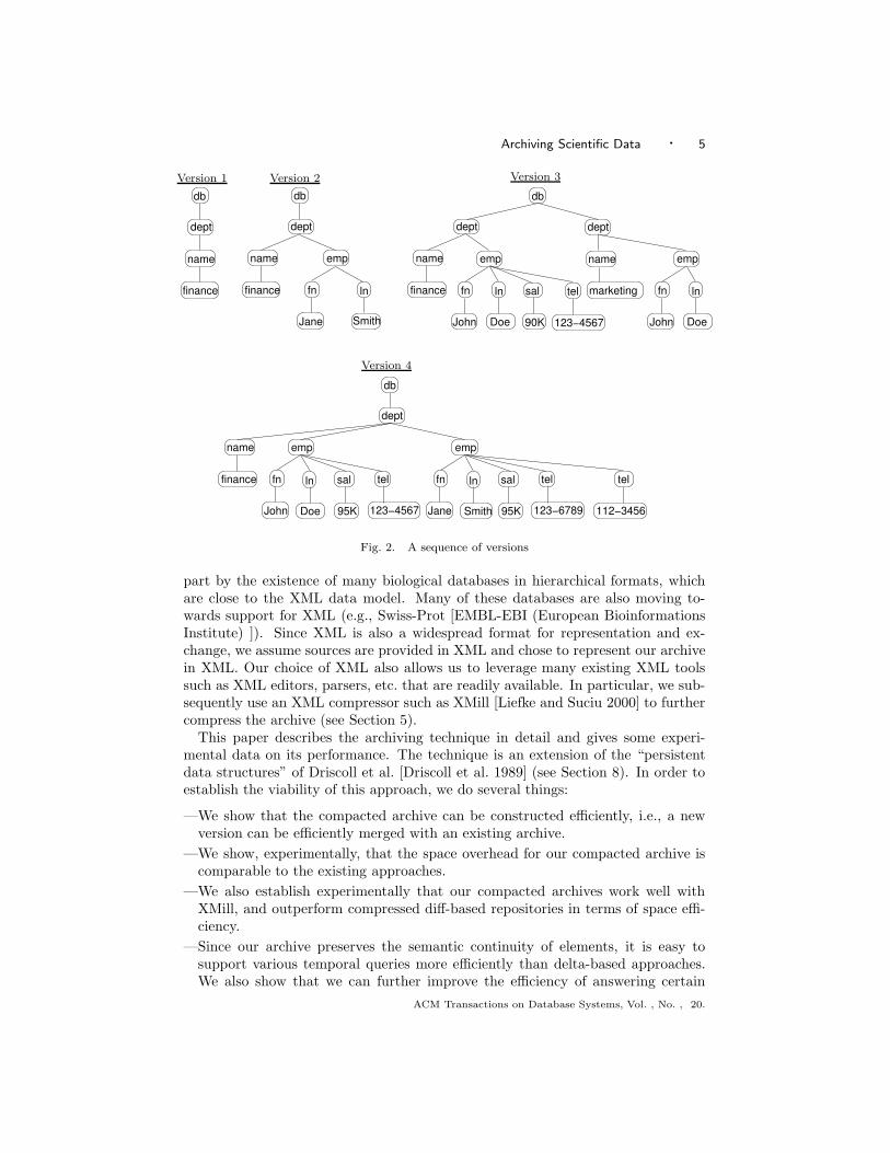
Fig. 8. Illustration of Nested Merge.
Keyed nodes of an archive are annotated in the same way. In addition, wehandle the timestamp tags as follows. Whenever “...<T t=...>V </T>...” occurswhere t=... is the timestamp and V represents the contents within the tag T, theroot nodes of V are annotated with timestamp t=... if they are keyed. Otherwise,V must contain nodes beneath frontier nodes. In this case, V remains as a subtreeof node <T t=...>.
Example 4.1. Figure 4 shows an example. Observe that the timestamp t=[3-4]is annotated on the emp{fn=John, ln=Doe} node. However, since 90K and 95Kare beyond frontier nodes, they continue to exist under their respective timestampnodes.
4.2 Nested Merge
Nested Merge is used for archiving documents where the order among keyed nodesdoes not matter. We first describe the main idea behind Nested Merge beforedescribing the algorithm in detail below. The main idea behind nested merge isrecursively to merge nodes in D (the incoming version) to nodes in A (the archive)that have the same key value, starting from the root. When a node y from Dis merged with a node x from A, the timestamp of x is augmented with i, thenew version number. The subtrees of nodes x and y are then recursively mergedtogether. Nodes in D that do not have corresponding nodes in A are simply addedto A with the new version number as its timestamp. Nodes in A that no longerexists in the current version D will have their timestamps terminated appropriately,i.e., these nodes do not contain timestamp i.
Example 4.2. Figure 8 illustrates the basic idea of Nested Merge. An arrowbetween a node in the archive and a node in the version indicates that they arecorresponding nodes, i.e., they have the same key value. Corresponding nodes aremerged together in the new archive and their timestamps are augmented with thelatest version number, i.e., number 12. Since the b element no longer exists inVersion 12, its timestamp is not augmented with the latest version number in thenew archive. On the other hand, since c first exists in Version 12, a new c element iscreated in the new archive with the timestamp t=[12]. Assuming that a is a frontiernode, Nested Merge will detect that the contents of the a element in the archiveand that in the incoming version are different, i.e., <d/><e/><f/> is not the same
ACM Transactions on Database Systems, Vol. , No. , 20.

Archiving Scientific Data · 15
as <d/><e/><g/> according to value equality. Hence, although there are clearlycommon elements among the contents, they are stored separately under differenttimestamp nodes in the new archive.
Value Equality. Before we describe the algorithm Nested Merge, we shall recallthe definition of value equality (also described in Appendix A), which is used incomparing key values of nodes in Nested Merge. Recall that the value of a nodeis defined according to its type. If a node is a text node (T-node), the value is itstext string. If a node is an attribute node (A-node) that has attribute name l andstring v, its value is the pair (l, v). The value of an element node (E-node) consistsof two things: (1) a possibly empty list of values of its E and T children nodesaccording to the document order, and (2) a possibly empty set of values of its Achildren nodes. A node n1 is value equal to a node n2, denoted as n1 =v n2, if theyagree on their value, i.e., intuitively, the trees rooted at the nodes are isomorphicby an isomorphism that is identity on string values.
In the following discussion, we assume that A and D are already annotated withkeys as described in the previous section. We assume the archive A contains versions1 through i−1 and D is the new version (version i), which respects key specificationK, to be archived into A. To simplify discussion, we assume that elements in theincoming version or archive, except timestamp elements, do not contain attributes.The archive A is assumed to contain a single root node rA even when no versionsare present. For any node x in A, let time(x) denote the timestamps annotatedon node x. Before any version is merged into A, time(rA) exists as an emptyset. Let label(x) denote the full label of a node x, including its key value butexcluding timestamp annotations. For example, the label of the emp node of JohnDoe in Figure 4 is emp{fn=John, ln=Doe}. In general, the label of a node hasthe form l(p1 = v1, ..., pk = vk). The labels of two nodes, l{p1 = v1, ..., pk = vk}and l′{p1 = v′1, ..., pk = v′k}, are equal if the corresponding tag names are identical(l = l′) and key values are the same (v1 =v v′1, ..., vk =v v′k). Otherwise, theyare not the same. Let rD denote the virtual root of D where label(rD) is identicalto label(rA) and the tree representation of D is contained as a subtree of rD . Letchildren(x) denote the sequence of children nodes of x. Let xml(x) denote theXML representation of the entire tree rooted at x. We invoke the algorithm withthe following arguments, Nested Merge(rA, rD, {}). The last argument containsinherited timestamp, initially empty.Algorithm Nested Merge(x, y, T )
If time(x) exists, thenadd i to time(x),let T be time(x).
If y is a frontier node thenIf every node in children(x) is not a timestamp node, then
If x 6=v y, thencreate timestamp node t1 (i.e., <T t="T − {i}">) and attach children(x) to t1,create timestamp node t2 (i.e., <T t="i">) and attach children(y) to t2,attach t1 and t2 as children nodes of x.
ElseIf there exists a node x′ in children(x) such that children(x′)=v children(y), then
ACM Transactions on Database Systems, Vol. , No. , 20.

16 · Buneman, Khanna, Tajima, and Tan
add i to time(x′).Else
create timestamp node t1 (i.e., <T t="i">) and attach children(y) to t1,attach t1 as child node of x.
ElseLet XY = {(x′, y′) | x′ ∈ children(x), y′ ∈ children(y), label(x′) = label(y′)}.Let X ′ denote the rest of the nodes in children(x) that do not occur in XY andY ′ denote the rest of the nodes in children(y) that do not occur in XY .For every pair (x′, y′) ∈ XY
(a) Nested Merge(x′, y′, T )For every x′ ∈ X ′
(b) If time(x′) does not exist, then let time(x′) be T − {i}.For every y′ ∈ Y ′
(c) Let time(y′) = {i} and attach y′ as a child node of x.
The algorithm first determines the current timestamp. It is i added to time(x)if time(x) exists. Otherwise, the timestamp is inherited from its parent. Observethat time(rA) always exists. It is a property of the algorithm that label(x) =label(y) whenever Nested Merge(x, y, T ) is invoked. The algorithm then proceedsby checking if y is a frontier node.
Frontier nodes are handled specially because there are no keyed nodes beyondfrontier nodes. Thus the recursive merging of identical nodes no longer applies forthe descendents of frontier nodes. The children nodes of any frontier node have theproperty that either they are all timestamp nodes or none of them is a timestampnode. In Figure 4, sal of John Doe is an example of a frontier node whose childrenare all timestamp nodes, tel of John Doe is a frontier node none of whose childrenare timestamp nodes. The transition from having no timestamp children nodesto all timestamp children nodes occurs when an incoming version is such that thecontent of the frontier node to be merged differs from that in the archive. Considerthe last archive in Figure 9 which contains versions 1-3. When version 4 is merged,sal of John Doe in version 4 differs from that in the archive containing versions 1-3.Hence, timestamps are used to enclose the salary values at the respective times.The resulting archive is shown in Figure 4.
If y is not a frontier node, we “partition” nodes in children(x) and children(y)into three sets. (1) The first set, XY , contains pairs of nodes from children(x) andchildren(y) respectively with equal key values. Observe that by the property ofkeys, for every node in children(x), there can be at most one node in children(y)with an equal key value. (2) The second and third sets are X ′ and Y ′. The set X ′
(resp. Y ′) consists of nodes in children(x) (resp. children(y)) where there does notexist any node in children(y) (resp. children(X)) with an equal key value.
Nested merge is recursively called on pairs of nodes in XY , inheriting the currenttimestamp T . To ensure that nodes of X ′ no longer exist at time i, timestamp Texcluding i is annotated on nodes of X ′ if they do not already contain timestampannotations that terminate earlier than i. Subtrees rooted at nodes of Y ′ areattached as a subtrees of x and they are annotated with timestamp i since theyonly begin to exist at time i.
ACM Transactions on Database Systems, Vol. , No. , 20.
Archiving Scientific Data · 17
root, t=[]
db
dept
name
finance
root, t=[1]
name
finance fn ln
SmithJane
db
root, t=[1,2]
dept
emp, t=[2]
dept
db
root, t=[1−3]
dept, t=[3]
name
finance fn
John
ln
Doe 123−4567
telsal
90K
emp, t=[3] name
marketing fn
emp
John
ln
Doe
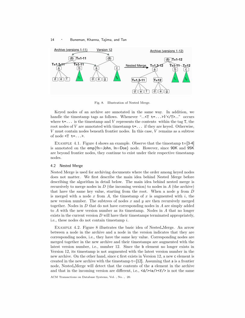
Fig. 9. States of the archive as versions 1-3 are merged. Keys of nodes are omitted.
Figure 9 together with Figure 4 shows the evolution of the archive as versions 1to 4 of Figure 2 are added.Analysis. We analyze the running time of Nested Merge to show that it isO(αN log N), where N = max(NA, ND), NA and ND are the number of nodesin A and D respectively, and α is the maximum time it takes to compare the labelsof two nodes or test if two nodes are value equal. We assume the set of frontierpaths are kept in a hash table and hashing will allow us to determine if a givenpath (or node) is a frontier path in expected constant time. Let dA and dD be themaximum degree of A and D respectively. Hence children(x) and children(y) canbe determined in dA and dD time. According to the algorithm, if y is a frontiernode, so is x. The first If statement following the condition that y is a frontiernode in the algorithm executes in O(dA) time since there are at most dA childrennodes in children(x). The second If statement executes in α time. The third Ifstatement executes in O(α ∗ dA) time assuming that the time to test whether thesequence of nodes in children(x′) is value equal to the respective sequence of nodesin children(y) takes less time than testing whether x′ =v y, which takes α time atworst. The rest of the statements take take at worst O(dA + dD) time to attachnodes to t1 or t2 respectively. Hence the statements on the condition that y is afrontier node executes in O(α(dA + dD)) time.
In case y is not a frontier node, the algorithm proceeds to determine XY , X ′,and Y ′ and appropriate actions, (a), (b), and (c), are taken for nodes in each set. Infact, one does not have to determine XY , X ′ and Y ′ naively. Our implementation
ACM Transactions on Database Systems, Vol. , No. , 20.

18 · Buneman, Khanna, Tajima, and Tan
assumes that children(x) and children(y) are sorted in ascending order according totheir key values and a merge-sort is done on the sorted nodes: Start with the firstnode of each sorted sequence children(x) and children(y). Call them x′ and y′. (1)If label(x′)=lablabel(y′), then perform action (a). (2) If label(x′)<lablabel(y′), thenperform the action (b) on x′ and let x′ be the next node in the sequence children(x).(3) Otherwise, perform action (c) on y′ and let y′ be the next node in the sequencechildren(y). We repeat this procedure until we run out of nodes on either sequence.If children(x) (resp. children(y)) is empty first, we perform action (c) (resp. (b))on the rest of the nodes in children(y) (resp. children(x)). Since every node in Aand D is sorted at some point and a merge sort is performed, Nested Merge takesO(αN log N) time.
Observe that in the description above, we have used “≤lab” to compare the labelsof two nodes. We define “≤lab” for labels of nodes next. Let label(x) be l1(p1 = v1,..., pk = vk) and label(y) be l2(p
′
1 = v′1, ..., p′l = v′l), where the key path valuesare lexicographically ordered according to pis and p′is. Then, label(x)<lablabel(y)if (i) l1 < l2, or (ii) l1 = l2 and k < l, or (iii) l1 = l2, k = l, pi = p′i, vi =v v′ifor all i ∈ [1, j − 1], j ∈ [1, k], and pj < p′j , or (iv) l1 = l2, k = l, pi = p′i,vi =v v′i for all i ∈ [1, j − 1], j ∈ [1, k], pj = p′j , and vj <v v′j . The label of twonodes are equal (label(x)=lablabel(y)) if l1 = l2, k = l, pi = p′i, vi =v v′i for alli ∈ [1, k]. The definition of “≤v” for XML values can be found in Appendix A.Notice that had we computed fingerprints, the process of determining whetherlabel(x) is less than label(y) will compare the fingerprints vj and v′j instead ofactual XML values. The use of fingerprints for ordering nodes does not affectcorrectness since we use the same ordering on nodes in the archive and versionand all that really matters in Nested Merge is that nodes with identical key values(therefore identical fingerprints) are merged together.Further Compaction. To obtain a further compact archive representation, onecan apply diff-based techniques on values beneath frontier nodes. Within the fron-tier node, we represent the contents that remain the same across versions only onceand mark the parts that differ by timestamps. This approach is much like the onethat SCCS [Rochkind 1975] adopts. In this way, instead of representing values ofthese nodes under the respective timestamps, we represent only their difference.The advantage of this technique arises when values differ only slightly across ver-sions.
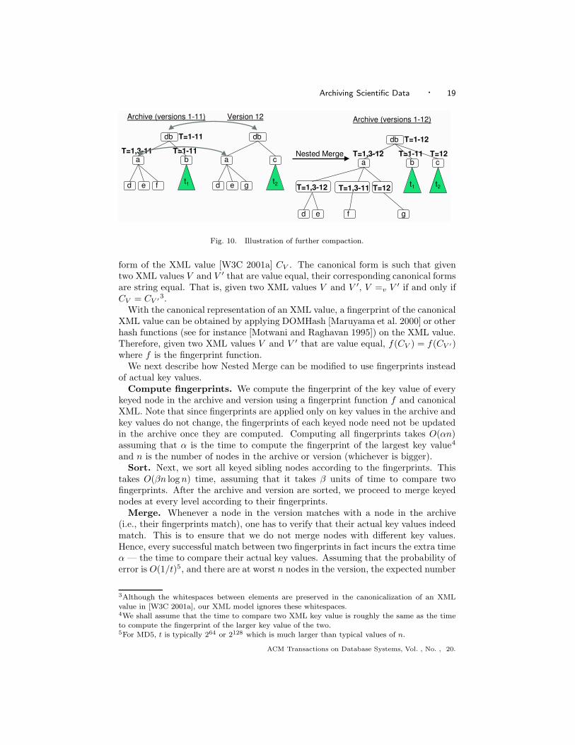
Example 4.3. Going back to the illustration for Nested Merge in Example 4.2,Figure 10 shows the resulting archive if further compaction is applied. Observe thatelements d and e occur only once in the output archive under further compactionsince the difference between the values of the frontier node a in the archive andincoming version is only on the last element. As before, we use timestamps tomark the existence of the nodes at various times.
4.3 The fingerprint of an XML value
In this section, we show how one can adapt Nested Merge to use fingerprints insteadof actual key values so that the version is archived correctly even when collisions offingerprints may occur.
To compute the fingerprint of an XML value V , we first obtain the canonical
ACM Transactions on Database Systems, Vol. , No. , 20.
Archiving Scientific Data · 19
db
a b
d e f t1
Archive�(versions�1-11)
db
a c
d e g t2
Version�12
Nested�Merge
T=1-11
T=1-11T=1,3-11db
a b
d e f
t1
Archive�(versions�1-12)
T=1-12
T=1-11c
t2
T=12T=1,3-12
T=1,3-12 T=12
g
T=1,3-11
Fig. 10. Illustration of further compaction.
form of the XML value [W3C 2001a] CV . The canonical form is such that giventwo XML values V and V ′ that are value equal, their corresponding canonical formsare string equal. That is, given two XML values V and V ′, V =v V ′ if and only ifCV = CV ′
3.With the canonical representation of an XML value, a fingerprint of the canonical
XML value can be obtained by applying DOMHash [Maruyama et al. 2000] or otherhash functions (see for instance [Motwani and Raghavan 1995]) on the XML value.Therefore, given two XML values V and V ′ that are value equal, f(CV ) = f(CV ′)where f is the fingerprint function.
We next describe how Nested Merge can be modified to use fingerprints insteadof actual key values.
Compute fingerprints. We compute the fingerprint of the key value of everykeyed node in the archive and version using a fingerprint function f and canonicalXML. Note that since fingerprints are applied only on key values in the archive andkey values do not change, the fingerprints of each keyed node need not be updatedin the archive once they are computed. Computing all fingerprints takes O(αn)assuming that α is the time to compute the fingerprint of the largest key value4
and n is the number of nodes in the archive or version (whichever is bigger).Sort. Next, we sort all keyed sibling nodes according to the fingerprints. This
takes O(βn log n) time, assuming that it takes β units of time to compare twofingerprints. After the archive and version are sorted, we proceed to merge keyednodes at every level according to their fingerprints.
Merge. Whenever a node in the version matches with a node in the archive(i.e., their fingerprints match), one has to verify that their actual key values indeedmatch. This is to ensure that we do not merge nodes with different key values.Hence, every successful match between two fingerprints in fact incurs the extra timeα — the time to compare their actual key values. Assuming that the probability oferror is O(1/t)5, and there are at worst n nodes in the version, the expected number
3Although the whitespaces between elements are preserved in the canonicalization of an XMLvalue in [W3C 2001a], our XML model ignores these whitespaces.4We shall assume that the time to compare two XML key value is roughly the same as the timeto compute the fingerprint of the larger key value of the two.5For MD5, t is typically 264 or 2128 which is much larger than typical values of n.
ACM Transactions on Database Systems, Vol. , No. , 20.

20 · Buneman, Khanna, Tajima, and Tan
of collisions for any node in the archive is therefore O(n/t). Therefore, at worstevery node in the version is compared with O(1+n/t) nodes in the archive during themerge process. Hence, the merge phase takes expected time O((β + α)(n + n2/t)).
We next compare the total “work” done when Nested Merge uses fingerprintswith the total “work” done when Nested Merge does not use fingerprints. Thetotal work done when Nested Merge uses fingerprints is
—Compute fingerprints. O(αn) for computing fingerprints of nodes in archiveand version.
—Sort. O(βn log n) for sorting nodes in archive and version.
—Merge. O((β + α)(n + n2/t) expected time for merging nodes in the version tothe archive.
The total work done when Nested Merge does not use fingerprints is
—Sort. O(αn log n) for sorting nodes in the archive and version.
—Merge. O(αn) for merging nodes in the version to archive.
Since a fingerprint is smaller than the size of the actual key value (β < α) and t istypically larger than n, the total work done in either case is roughly the same. Hencethe difference in total work done is essentially the time to compute fingerprints andsort nodes in the former case versus the time to sort nodes using actual key valuesin the latter case.
5. EXPERIMENTAL RESULTS
The main purpose of our experiments is to answer the following question: Howdoes the storage space performance of our technique compare with traditional diff-based + sequence-of-delta approaches? Our experiments show that our archiverequires only slightly more space than those existing approaches on real scientificdata. Moreover, our results also show that our compressed archive is more spaceefficient than any compressed delta-based repository. There are many variants ofdelta-based approaches but we identified two likely competitive candidates: (1) theincremental diff approach that stores the first version and diffs of every successivepairs of versions in a repository, and (2) the cumulative diff approach that storesthe first version and diffs of every version from the first version.
An alternative to the incremental diff approach is to store the last version to-gether with successive backward diffs. Whether with the forward or backward diffapproach, the size of the repositories should be the same since each element ap-pears exactly once in some diff and in the first (or last) version. Thus, we focusour attention on the forward diff approach and simply refer to it as the incrementaldiff approach. For similar reasons, the size of a cumulative backward diff repositoryshould be the same as that of the forward cumulative repository. Since the back-ward cumulative diff approach involves reconstructing all cumulative diffs whenevera new version arrives, we focus our attention instead on the forward cumulative diffapproach and simply refer to it as the cumulative diff approach.
Cumulative diffs is obviously worse than incremental diffs in storage efficiency.However, it has the advantage of being fast in retrieving any version: Any versioncan be retrieved by one application of an edit script. Hence if the storage space
ACM Transactions on Database Systems, Vol. , No. , 20.

Archiving Scientific Data · 21
required by cumulative diffs is not far from that required by incremental diffs, cumu-lative diffs would be a tougher competitor for us. Our experiments, however, showthat cumulative diffs quickly suffers from the large storage space when the numberof versions gets larger as shown later. Henceforth, we concentrate on comparisonsbetween our archive and the incremental diff approach.
In addition to the choice of incremental diffs or cumulative diffs, we also havea choice of tree diffs or line diffs. Tree diffs have been extensively studied [Zhangand Shasha 1989; 1990; Chawathe et al. 1996; Chawathe and Garcia-Molina 1997;Cobena et al. 2001] and we used XML-Diff [XMLTREEDIFF ], which is imple-mented for XML and is downloadable from the Web. However, when comparedwith line diff, XML-Diff incurred a significantly higher space overhead (and it wasalso not robust: We could only run it on some of our data). Since our XML datais formatted in such a way that each element is represented by one or more consec-utive lines separate from other elements, line diff gives a compact representationfor small changes. For this reason, we chose line diff for the comparison. In all ourexperiments, we used the standard unix diff command with “-d” option to computethe smallest edit scripts. Hence, the sizes of our diff repositories are always thesmallest possible.
Since each version of our data is large and our basic archiver is an in-memoryalgorithm, we quickly ran out of memory on a machine with 256MB memory. Toovercome the memory limitation, we hashed our experimental data into “chunks”based on the values of keys. An incoming version is partitioned in the same manner,and we apply our archiver to the corresponding chunks of the archive and theincoming version. Since we never merge elements with different key values, we canobtain the archive of the whole data by merging the archive and the version chunkby chunk, and concatenating the results. Since our concern was storage space,what we did to overcome the memory limitation was done in order to obtain aquick verification of how our archiving technique compares to conventional diff-based techniques. We show how to extend Nested Merge to an external memoryalgorithm in Section 6 to handle large files. We note here that unix diff (line diff)also ran out of memory on large files. Therefore we applied unix diff on versions ofthe respective chunks as well.
We also examined how our approach and other approaches perform in combi-nation with compression techniques. We compress the diff-based repositories withgzip (a standard file compression tool) and we compress our archives with XMill(an XML compression tool) [Liefke and Suciu 2000]. We also experimented withcompressing cumulative diffs with gzip since compressed cumulative diffs may besmall. As another possible competitor, we also put all the versions side by side intoone XML tree and compress it with XMill. Both gzip and XMill were run with“-9” option to give the best possible compression.
In the following graphs in this section, line version shows the size of each version,and line archive shows the size of our archives storing up to each version. LineV1+inc diffs shows the size of incremental diff repositories, i.e., the total size of thefirst version and all the incremental diffs, and line V1+cumu diffs shows the size ofcumulative diff repositories. Line gzip(V1+incremental diffs) and line gzip(V1+cumudiffs) refer to the size of incremental diff repository and cumulative diff repository
ACM Transactions on Database Systems, Vol. , No. , 20.
22 · Buneman, Khanna, Tajima, and Tan
Size (bytes) x 106 Size (bytes) x 109
OMIM Data
V1+cumulative_diffsarchiveV1+incremental_diffsversion
size (bytes) x 106
# of versions0.00
10.00
20.00
30.00
40.00
50.00
60.00
70.00
80.00
90.00
100.00
110.00
120.00
130.00
140.00
150.00
160.00
170.00
180.00
190.00
200.00
210.00
220.00
0.00 20.00 40.00 60.00 80.00 100.00
SwissProt Data
V1+cumulative_diffsarchiveV1+successive_diffsversion
size (bytes) x 109
version sequence0.00
0.20
0.40
0.60
0.80
1.00
1.20
1.40
1.60
1.80
2.00
2.20
2.40
2.60
2.80
3.00
0.00 5.00 10.00 15.00 20.00
V1+
cum
udi
ffs
archive
V1+inc diffs version
V1+
cum
udiff
s
arch
ive
V 1+incdiffs
version
Number of Versions
(a) OMIM (over 3 − 4 months) (b) Swiss-Prot (over ≈ 5 yrs)
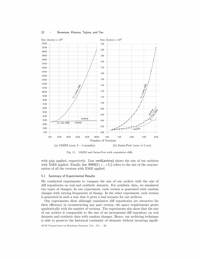
Fig. 11. OMIM and Swiss-Prot with cumulative diffs.
with gzip applied, respectively. Line xmill(archive) shows the size of our archiveswith XMill applied. Finally, line XMill(V1+...+Vi) refers to the size of the concate-nation of all the versions with XMill applied.
5.1 Summary of Experimental Results
We conducted experiments to compare the size of our archive with the size ofdiff repositories on real and synthetic datasets. For synthetic data, we simulatedtwo types of changes; In one experiment, each version is generated with randomchanges with varying frequencies of change. In the other experiment, each versionis generated in such a way that it gives a bad scenario for our archiver.
Our experiments show although cumulative diff repositories are attractive fortheir efficiency in reconstructing any past version, the space requirements growsquadratically with the number of versions. The experiments also show that the sizeof our archive is comparable to the size of an incremental diff repository on realdatasets and synthetic data with random changes. Hence, our archiving techniqueis able to preserve the historical continuity of elements without incurring signifi-
ACM Transactions on Database Systems, Vol. , No. , 20.

Archiving Scientific Data · 23
Size (bytes) x 106 Size (bytes) x 109
OMIM Data
archiveV1+incremental_diffsversiongzip(V1+cumulative_diffs)xmill(V1+...+Vi)gzip(V1+incremental_diffs)xmill(archive)
size (bytes) x 106
# of versions
0.00
5.00
10.00
15.00
20.00
25.00
30.00
35.00
40.00
45.00
50.00
55.00
60.00
65.00
70.00
0.00 20.00 40.00 60.00 80.00 100.00
SwissProt Data
archiveV1+successive_diffsversiongzip(V1+cumulative_diffs)xmill(V1+...+Vi)gzip(V1+successive_diffs)xmill(archive)
size (bytes) x 106
version sequence0.00
50.00
100.00
150.00
200.00
250.00
300.00
350.00
400.00
450.00
500.00
550.00
600.00
650.00
700.00
750.00
800.00
850.00
900.00
0.00 5.00 10.00 15.00 20.00
archive, V1+inc diffs
version
gzip
(V1+
cum
udiff
s)
xmill(V1 + ...Vi)
gzip(V1+inc diffs)
xmill(archive)
arch
ive
V1+
inc
diff
s
versio
n
gzip(V
1+
cum
udiffs)
xmill(V
1
+...
+V i
)
gzip(V
1+inc
diffs)
xmill(archi
ve)
Number of Versions
(a) OMIM (over 3 − 4 months) (b) Swiss-Prot (over ≈ 5 yrs)
Fig. 12. Storage space of OMIM and Swiss-Prot with incremental diffs.
cant space overhead when compared with diff-based repositories. Furthermore, weshow that our compressed archive outperforms compressed diff repositories in allscenarios (real or synthetic). For synthetic data where we generated bad scenariosfor our archiver, our archive indeed takes up much more space than an incrementaldiff repository as expected. Suprisingly, however, our compressed archive continuesto outperform the compressed incremental diff repository even under such circum-stances. Hence, if space is the main concern, we are likely to do better archivingwith our technique and compressing with XML compression tools.
5.2 Comparison with Cumulative Diffs
We first show that although cumulative diff has the advantage of retrieving anypast version fast, it quickly suffers from the drawback of incurring large amounts ofstorage space when it is applied to real data. Figure 11 shows the result of applyingthe cumulative diff approach to OMIM [OMIM 2000] and Swiss-Prot [Bairoch and
ACM Transactions on Database Systems, Vol. , No. , 20.
24 · Buneman, Khanna, Tajima, and Tan
Size (bytes) x 106 Size (bytes) x 106
Auction Data (05)
archiveV1 + incremental diffsversiongzip(V1 + cumulative diffs)xmill(V1+...+Vi)gzip(V1 + incremental diffs)xmill(archive)
size (bytes) x 106
version sequence
0.00
1.00
2.00
3.00
4.00
5.00
6.00
7.00
8.00
9.00
10.00
11.00
12.00
13.00
14.00
15.00
16.00
17.00
18.00
19.00
0.00 5.00 10.00 15.00 20.00
Auction Data (30)
archiveV1 + incremental diffsversiongzip(V1 + cumulative diffs)xmill(V1+...+Vi)gzip(V1 + incremental diffs)xmill(archive)
size (bytes) x 106
version sequence
0.00
5.00
10.00
15.00
20.00
25.00
30.00
35.00
40.00
45.00
50.00
55.00
60.00
65.00
70.00
75.00
0.00 5.00 10.00 15.00 20.00
archiv
e
V1+inc
diffs
versiongz
ip(V
1+
cum
udi
ffs)
xmill(V1+ ... + Vi)
gzip(V1+inc diffs)
xmill(archive)
arch
ive
V1+
inc
diffs
version
gzip(V
1+
cum
udiffs)
xmill(V
1+
...+
Vi)
gzip
(V1+
inc
diffs)
xmill(arch
ive)
Number of Versions
(a) 1.66%/1.66%/1.66% change ratio (b) 10%/10%/10% change ratio
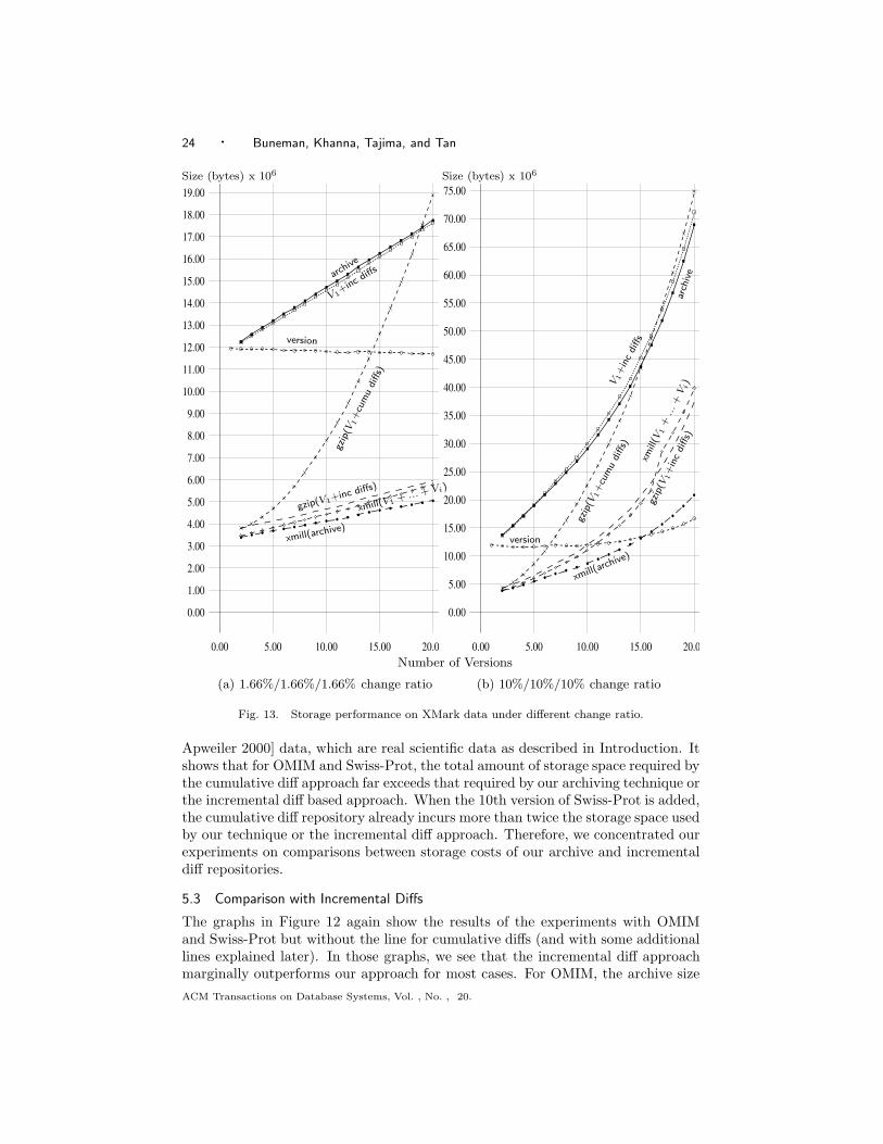
Fig. 13. Storage performance on XMark data under different change ratio.
Apweiler 2000] data, which are real scientific data as described in Introduction. Itshows that for OMIM and Swiss-Prot, the total amount of storage space required bythe cumulative diff approach far exceeds that required by our archiving technique orthe incremental diff based approach. When the 10th version of Swiss-Prot is added,the cumulative diff repository already incurs more than twice the storage space usedby our technique or the incremental diff approach. Therefore, we concentrated ourexperiments on comparisons between storage costs of our archive and incrementaldiff repositories.
5.3 Comparison with Incremental Diffs
The graphs in Figure 12 again show the results of the experiments with OMIMand Swiss-Prot but without the line for cumulative diffs (and with some additionallines explained later). In those graphs, we see that the incremental diff approachmarginally outperforms our approach for most cases. For OMIM, the archive size
ACM Transactions on Database Systems, Vol. , No. , 20.

Archiving Scientific Data · 25
Size (bytes) x 106 Size (bytes) x 106
Auction Data (05)
archiveV1 + incremental diffsversiongzip(V1 + cumulative diffs)xmill(V1+...+Vi)gzip(V1 + incremental diffs)xmill(archive)
size (bytes) x 106
version sequence
0.00
1.00
2.00
3.00
4.00
5.00
6.00
7.00
8.00
9.00
10.00
11.00
12.00
13.00
14.00
15.00
16.00
0.00 5.00 10.00 15.00 20.00
Auction Data (30)
archiveV1 + incremental diffsversiongzip(V1 + cumulative diffs)xmill(V1+...+Vi)gzip(V1 + incremental diffs)xmill(archive)
size (bytes) x 106
version sequence
0.00
2.00
4.00
6.00
8.00
10.00
12.00
14.00
16.00
18.00
20.00
22.00
24.00
26.00
28.00
30.00
32.00
34.00
36.00
38.00
0.00 5.00 10.00 15.00 20.00
archiv
e
V1+inc diffs
version
gzip(V1+cumu diffs)
xmill(V1 + ... + Vi)
gzip(V1+inc diffs)
xmill(archive)
arch
ive
V1+inc diffs
version
gzip(V1+cumu diffs)
xmill(V1 + ... + Vi)gzip(V1+inc diffs)
xmill(archive)
Number of Versions
(a) 1.66%/1.66%/1.66% change ratio (b) 10%/10%/10% change ratio
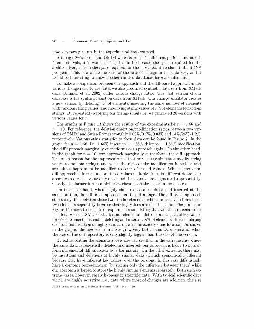
Fig. 14. Storage performance on XMark data with insertion and deletion of highly similar elements.
is never 1% more than the size of incremental diffs, and for Swiss-Prot, the archivesize is never 8% more than the size of incremental diffs.
In the graph for Swiss-Prot, the size of our archive grows quadratically or evenfaster. This is because the size of each version grows very fast, and as it grows, theamount of change between two consecutive versions also grows. Compared withthe incremental diff approach, which logically achieves the smallest space cost, ourapproach is not doing much worse.
Observe that the data stored in our approach and the diff approach are essentiallythe same (although they are organized in different ways, i.e., grouped by elementsversus grouped by time). The small difference between the storage space in thetwo approaches mainly comes from the difference between the size of timestampsin our archives and the size of “markers” in diff scripts. If we have a huge numberof changes of very small data, such as a text data of length 1, the ratio of thatdifference to the size of the archive can be considerable. Such an extreme situation,
ACM Transactions on Database Systems, Vol. , No. , 20.
26 · Buneman, Khanna, Tajima, and Tan
however, rarely occurs in the experimental data we used.
Although Swiss-Prot and OMIM were recorded for different periods and at dif-ferent intervals, it is worth noting that in both cases the space required for thearchive diverges from the space required for the most recent version at about 15%per year. This is a crude measure of the rate of change in the database, and itwould be interesting to know if other curated databases have a similar rate.
To make a comparison between our approach and the diff-based approach undervarious change ratio to the data, we also produced synthetic data sets from XMarkdata [Schmidt et al. 2002] under various change ratio. The first version of ourdatabase is the synthetic auction data from XMark. Our change simulator createsa new version by deleting n% of elements, inserting the same number of elementswith random string values, and modifying string values of n% of elements to randomstrings. By repeatedly applying our change simulator, we generated 20 versions withvarious values for n.
The graphs in Figure 13 shows the results of the experiments for n = 1.66 andn = 10. For reference, the deletion/insertion/modification ratios between two ver-sions of OMIM and Swiss-Prot are roughly 0.02%/0.2%/0.03% and 14%/26%/1.2%,respectively. Various other statistics of these data can be found in Figure 7. In thegraph for n = 1.66, i.e. 1.66% insertion + 1.66% deletion + 1.66% modification,the diff approach marginally outperforms our approach again. On the other hand,in the graph for n = 10, our approach marginally outperforms the diff approach.The main reason for the improvement is that our change simulator modify stringvalues to random strings, and when the ratio of the modification is high, a textsometimes happens to be modified to some of its old values. While incrementaldiff approach is forced to store those values multiple times in different deltas, ourapproach stores the value only once, and timestamps are augmented appropriately.Clearly, the former incurs a higher overhead than the latter in most cases.
On the other hand, when highly similar data are deleted and inserted at thesame location, the diff-based approach has the advantage. The diff-based approachstores only diffs between those two similar elements, while our archiver stores thosetwo elements separately because their key values are not the same. The graphs inFigure 14 shows the results of experiments simulating that worst-case scenario forus. Here, we used XMark data, but our change simulator modifies part of key valuesfor n% of elements instead of deleting and inserting n% of elements. It is simulatingdeletion and insertion of highly similar data at the exactly same location. As shownin the graphs, the size of our archives grow very fast in this worst scenario, whilethe size of the diff repository is only slightly bigger than the size of one version.
By extrapolating the scenario above, one can see that in the extreme case wherethe same data is repeatedly deleted and inserted, our approach is likely to outper-form incremental diff approach by a big margin. On the other extreme, there maybe insertions and deletions of highly similar data (though semantically differentbecause they have different key values) over the versions. In this case diffs usuallyhave a compact representation (by storing only the difference between them) whileour approach is forced to store the highly similar elements separately. Both such ex-treme cases, however, rarely happens in scientific data. With typical scientific datawhich are highly accretive, i.e., data where most of changes are addition, the size
ACM Transactions on Database Systems, Vol. , No. , 20.

Archiving Scientific Data · 27
of our archive and the size of the diff-based repository would be roughly the same.The experimental results with OMIM data, changes to which is mainly addition asshown in Figure 7, verifies that observation.
5.4 Interaction with Compression
We have seen that incremental diff technique may outperform our technique interms of storage space. However, when compression is applied to both our archivesand incremental diff repositories, our archives use less storage space in most of ourexperiments. For both OMIM and Swiss-Prot (in Figure 12), we see that XMillapplied on our archive (xmill(archive) line) outperforms any other approaches, i.e.gzip(incremental-diff), gzip(cumulative-diff), and xmill(V1 + . . . + Vi), even duringthe times when the incremental diff repository is clearly smaller than our archivewithout compression. For instance, in Figure 12(b), as our archive starts to performworse than the incremental diff repository after Version 17, our compressed archivecontinues to outperform the compressed diff repository by a growing margin. Bythe time Version 20 of Swiss-Prot is added, the storage space used by our archive isclearly more than incremental-diff. However, gzip(incremental-diff) uses clearly morestorage space than xmill(archive) by about the same magnitude. It seems the marginbetween gzip(incremental-diff) and xmill(archive) is bigger when the change ratio ishigh. It is bigger in Figure 12(b) than in Figure 12(a), and within Figure 12(b), itis bigger at Version 10. . . 20 than at Version 1. . . 10. The same characteristic canalso be seen in Figure 13.
This reversal of storage space efficiency occurs because our archive of XML datasets is again in XML format, and XMill can exploit this specific structure to obtain abetter compression ratio than general compression tools like gzip. XMill groups textdata according to the names of the elements in which they occur and compresseseach group separately. Since text data that belong to elements of the same nametend to be fairly similar, high compression ratios can usually be achieved.
Higher compression ratio of xmill(archive) can be seen even in the graphs of theworst-case scenario in Figure 14. In those graphs, xmill(archive) is smaller thangzip(incremental-diff) up to the points where our archive gets about 1.2 times largerthan the incremental diff repository (ver. 14 in (a) and ver. 3 in (b)). After thosepoints, the difference of the size of our archive and the diff repository seems outrunthe higher compression ratio of XMill.
Our graphs also show that a simple application of XMill to the concatenation ofall the versions does not work as well as our archive compressed with XMill (seelines xmill(V1 + ... + Vi) and xmill(archive)). Finally, the combination of gzip andcumulative diffs achieves a rather high compression ratio. However, it still does notperform as well as the XMill applied to our archive.
Remarks. In Figure 12(b), we reached the system file size limit of 231 whentrying to add Version 19 to V1+cumulative-diffs repository before applying gzip.The limit is also reached when trying to add Version 16 to the V1 + ... + V15
repository before XMill can be applied and hence the discontinuation in linesgzip(V1+cumulative-diffs) and xmill(V1 + ... + Vi) in this graph. In the same way, inFigure 12(a), xmill(V1 + ...+V80) reaches the limit. In addition, the stepping in thexmill(V1 + . . . + Vi) is due to the fact that xmill is using “dictionary compression”and is increasing the space allocation for the dictionary.
ACM Transactions on Database Systems, Vol. , No. , 20.

28 · Buneman, Khanna, Tajima, and Tan
6. EXTERNAL MEMORY NESTED MERGE
The algorithm Nested Merge, presented in Section 4.2, is an “in-memory” algo-rithm. Nested Merge assumes that the entire archive and version can be read intomemory before deciding which nodes can be merged. The smallest version in Swiss-Prot has about 2, 037, 292 nodes and can contain as many as 10, 903, 568 nodes. Ona machine with a standard amount of memory, Nested Merge clearly cannot han-dle such files. To overcome the memory limitation, one solution is to use PDOM(Persistent Document Object Model) [PDOM ]. PDOM provides DOM API to pro-cess XML documents that far exceed memory limits. However, the performance ofPDOM largely depends on how the XML file is fragmented, what indices are builtaccording to PDOM implementation and how the XML file is accessed.
In this section, we describe how one can extend Nested Merge to an externalmemory algorithm to handle data where the size of data may be much larger thanthe available memory. The main steps taken by the external memory archiver,which we outline here, are essentially the same as that described Section 4.External Memory Archiver
Input: An archive, a new version (to be merged into the archive), and a set ofkey specifications.Output: A new archive that contains the new version.
(1) Annotate nodes with their key values. Both the archive and new ver-sion are preprocessed so that, conceptually, every keyed node has its key valueimmediately associated with it. (See Section 6.1.)
(2) Sort archive and new version. The archive and new version are each sortedaccording to keys, i.e., all sibling nodes are ordered according to key values.(See Section 6.2.)
(3) Merge sorted archive with version. The archive and version are mergedtogether by making a single pass through both documents. (See Section 6.3.)
In the ensuing description, we let M be the total memory size and B be the sizeof a page (or 1 disk block). Let the total size of a version or archive (whichever islarger) be N . We are of course interested in the case when M < N . We assumethat every root-to-leaf path (including all key values of nodes along the path) inour document can fit in one page. This means h < B (which is generally truein practice), where h is the height of the document. For example, the heights ofOMIM, Swiss-Prot and XMark versions are 5, 6 and 12 respectively. The heightsof the respective archives is at worst twice (due to timestamp tags) the heights ofthe respective versions.
6.1 Annotate nodes with their key values
Prior to sorting a document according to key values, we first annotate every keyednode with its key value. Our implementation makes use of an internal representa-tion of an XML document similar to that used by XMill [Liefke and Suciu 2000].This step breaks an input document into three main types of files for subsequentprocessing: (1) an internal representation of the document, (2) a dictionary, and(3) keys files.
ACM Transactions on Database Systems, Vol. , No. , 20.
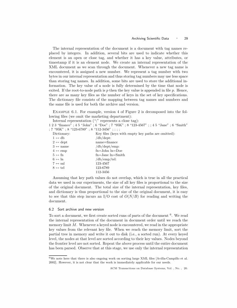
Archiving Scientific Data · 29
The internal representation of the document is a document with tag names re-placed by integers. In addition, several bits are used to indicate whether thiselement is an open or close tag, and whether it has a key value, attributes, ortimestamp if it is an element node. We create an internal representation of theXML document as we scan through the document. Whenever a new tag name isencountered, it is assigned a new number. We represent a tag number with twobytes in our internal representation and thus storing tag numbers may use less spacethan storing tag names. In addition, some bits are used to store the additional in-formation. The key value of a node is fully determined by the time that node isexited. If the root-to-node path is p then the key value is appended in file p. Hence,there are as many key files as the number of keys in the set of key specifications.The dictionary file consists of the mapping between tag names and numbers andthe same file is used for both the archive and version.
Example 6.1. For example, version 4 of Figure 2 is decomposed into the fol-lowing files (we omit the marketing department):
Internal representation (“;” represents a close tag):1 2 3 “finance” ; 4 5 “John” ; 6 “Doe” ; 7 “95K” ; 8 “123-4567” ; ; 4 5 “Jane” ; 6 “Smith”; 7 “95K” ; 8 “123-6789” ; 8 “112-3456” ; ; ; ;
Dictionary:1 ↔ db2 ↔ dept3 ↔ name4 ↔ emp5 ↔ fn6 ↔ ln7 ↔ sal8 ↔ tel
Key files (keys with empty key paths are omitted):/db/dept:name=finance/db/dept/emp:fn=John ln=Doefn=Jane ln=Smith/db/emp/tel:123-4567123-6789112-3456
Assuming that key path values do not overlap, which is true in all the practicaldata we used in our experiments, the size of all key files is proportional to the sizeof the original document. The total size of the internal representation, key files,and dictionary is thus proportional to the size of the original document, it is easyto see that this step incurs an I/O cost of O(N/B) for reading and writing thedocument.
6.2 Sort archive and new version
To sort a document, we first create sorted runs of parts of the document 6. We readthe internal representation of the document in document order until we reach thememory limit M . Whenever a keyed node is encountered, we read in the appropriatekey values from the relevant key file. When we reach the memory limit, sort thepartial tree in memory and write it out to disk (i.e., a sorted run). At every keyedlevel, the nodes at that level are sorted according to their key values. Nodes beyondthe frontier level are not sorted. Repeat the above process until the entire documenthas been parsed. Observe that at this stage, we use only the internal representation
6We note here that there is also ongoing work on sorting large XML files [Avilla-Campillo et al.2002]. However, it is not clear that the work is immediately applicable for our needs.
ACM Transactions on Database Systems, Vol. , No. , 20.

30 · Buneman, Khanna, Tajima, and Tan
and key files of the archive or version. Moreover, we only make a single pass throughthese files to create the sorted runs.
In the course of producing sorted runs, many root-to-leaf paths may be duplicatedacross the runs. Hence, the total size of all sorted runs may be larger than the sizeof the original document. For example, consider a document which has a long stema1, ..., am and many leaves b1, ..., bn as shown below.PSfrag replacements
a1 a1 a1a1
a2 a2 a2a2
am amam
am
b1 b1b2 b2bn bn
Original document Run 1 Run 2 Run n
It may happen that the memory limit is reached whenever a bi is read (Recallthat we assume every root-to-leaf path can fit in a page.). Therefore, each sortedrun produced consists of a1/.../am/bi. The stem a1/.../am is copied n times acrosseach sorted run. Since, in the worst scenario, each sorted runs begins with h units ofmemory already occupied by some root-to-leaf path (the point where the algorithmstops in the previous run), the number of sorted runs is bounded by O(N/(M −h)). Due to duplication, the total size of all sorted runs may have increased byO(hN/(M − h)). Hence we have used a total of O(N/B + hN/(B(M − h))) I/Osso far.
To obtain a sorted tree, we repeatedly merge the sorted runs until we end upwith one sorted run containing the entire tree. We start by placing a marker atthe root of each (M/B) − 1 trees in memory. Consider the markers at height 0(hence all markers initially), we output the marker node with the smallest label.Next, for every marker node whose label equals the smallest value, we advancethe marker to the next node of the tree (in document order). Observe that somemarkers will advance to their siblings while other markers will advance to theirchildren nodes. We repeat the process by considering markers occurring at thedeepest level in all runs. Everytime the output buffer is full, we simply write it outto disk and keep the path from the root to the last node we emitted. During themerge process, whenever a frontier node is encountered, we write out the subtreein the order which the runs are created. In this way, we ensure that the relativeorder of unkeyed nodes remains unchanged.
Since there are O(N/B+hN/(B(M−h))) number of pages in all sorted runs, eachmerge phase of (M/B)−1 sorted runs can be done with O(N/B+hN/(B(M −h)))I/Os. With N/(M − h) sorted runs at most, we have roughly
log(M/B)−1 N/(M − h) = log(M/B)−1 N/B − log(M/B)−1(M − h)/B
≤ log(M/B)−1 N/B
phases (h ≤ B and M > 2B). Therefore we use a total of O((N/B + hN/(B(M −h))) log(M/B)−1 N/B) I/Os.
ACM Transactions on Database Systems, Vol. , No. , 20.
Archiving Scientific Data · 31
6.3 Merge sorted archive and version
This step is very much like the previous step except that frontier nodes are han-dled differently — in a way similar to that described in the basic Nested Mergealgorithm. Given an archive A and version D, the external memory nested mergealgorithm first sorts A and D using the sorting procedure above. Call the sortedfiles A′ and D′ respectively. We let x and y denote nodes in A′ and D′, respectively.Initially, x is the root of A′ and y is a virtual root of D′ with the same key as xand x and y proceed through A′ and D′ in document order. We keep track of thetimestamp of the current node in A′ as we traverse the document. If label(x) <label(y), we output x and its entire subtree and attach the current timestamp tox. If label(x) > label(y) we output y and its entire subtree and attach timestampi (the new version number) to y. Otherwise label(x) = label(y). In this case, weoutput x and attach the current timestamp together with i if a timestamp originallyexists at x. Otherwise we output only x. If y is a frontier node, we proceed in asimilar way as described in Nested Merge algorithm in Section 4. Subsequently, wemove x and y to the next nodes of A′ and D′ in document order and repeat theprocedure. If we reach the end of A′ first, we output the entire subtree rooted aty with timestamp i and repeat with the next y until we reach the end of D′. Ifwe reach the end of D′ first, we output x and its entire subtree together with theexisting timestamp if any. We let x denote the next node in A′ and repeat untilwe reach the end of A′. Since this step makes one pass through the archive andversion, it incurs another O(N/B) I/Os.
We remark that a line-diff algorithm could also be extended so that it can handlelarge files. Given two versions that each far exceeds the available memory, a line-diffalgorithm can operate on “windows” of text, i.e., break each version into pages andcompute diff on corresponding pages of data of the two versions. Although the diffresult may not be optimal in this way, this method uses only O(N/B) I/Os.
7. EFFICIENTLY RETRIEVING A VERSION OR TEMPORAL HISTORY
We show how to retrieve a version and the temporal history of a keyed element effi-ciently. Our archive can already support these basic operations efficiently withoutbuilding any index structures. Here, we show that the complexity of these oper-ations can be further reduced by defining simple index structures on our archive:A version can be retrieved in time roughly proportional to the size of the ver-sion and the temporal history of a keyed element can be retrieved in time roughlyproportional to the size of its key.
7.1 Retrieving a Version
The structure of the archive is such that a simple scan through the archive canretrieve any version. Whenever a timestamp tag is encountered, we output thecontents of the timestamp element if the required version number can be found inthe timestamp. This process is likely to be more efficient than the sequence-of-delta approach whereby reconstructing a version may require many scans over thedata in order to apply all the relevant deltas. Our approach, however, still takestime proportional to the size of the archive even when the size of the version to beretrieved is much smaller than the archive. We describe here a simple scheme that
ACM Transactions on Database Systems, Vol. , No. , 20.
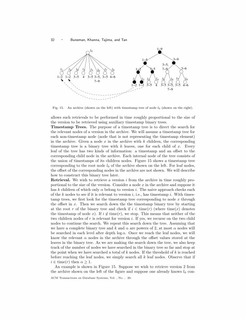
32 · Buneman, Khanna, Tajima, and Tan
3−5,7−9
3−5,7−9
3−5,7−9
1−2 1−2 3−543−5 3−5 4−6
1−2 1−2 3−5 4 3−5 3−5 4−6
1−2 3−5 3−6
3−91−5
1−9
PSfrag replacements
a1
a2
am
b1
b2
bn
Original document
Run 1Run 2Run n
l1
l1
l2
l2
l3
l3
l4
l4
l5
l5
l6
l6
l7
l7
l8
l8
l0
Fig. 15. An archive (shown on the left) with timestamp tree of node l0 (shown on the right).
allows such retrievals to be performed in time roughly proportional to the size ofthe version to be retrieved using auxiliary timestamp binary trees.Timestamp Trees. The purpose of a timestamp tree is to direct the search forthe relevant nodes of a version in the archive. We will assume a timestamp tree foreach non-timestamp node (node that is not representing the timestamp element)in the archive. Given a node x in the archive with k children, the correspondingtimestamp tree is a binary tree with k leaves, one for each child of x. Everyleaf of the tree has two kinds of information: a timestamp and an offset to thecorresponding child node in the archive. Each internal node of the tree consists ofthe union of timestamps of its children nodes. Figure 15 shows a timestamp treecorresponding to the root node l0 of the archive shown on the left. For leaf nodes,the offset of the corresponding nodes in the archive are not shown. We will describehow to construct this binary tree later.Retrieval. We wish to retrieve a version i from the archive in time roughly pro-portional to the size of the version. Consider a node x in the archive and suppose ithas k children of which only α belong to version i. The naive approach checks eachof the k nodes to see if it is relevant to version i, i.e., has timestamp i. With times-tamp trees, we first look for the timestamp tree corresponding to node x throughthe offset in x. Then we search down the the timestamp binary tree by startingat the root r of the binary tree and check if i ∈ time(r) (where time(x) denotesthe timestamp of node x). If i 6∈ time(r), we stop. This means that neither of thetwo children nodes of r is relevant for version i. If yes, we recurse on the two childnodes to continue the search. We repeat this search down the tree. Assuming thatwe have a complete binary tree and k and α are powers of 2, at most α nodes willbe searched in each level after depth log α. Once we reach the leaf nodes, we willknow the relevant α nodes in the archive through the offset values stored at theleaves in the binary tree. As we are making the search down the tree, we also keeptrack of the number of nodes we have searched in the binary tree so far and stop atthe point when we have searched a total of k nodes. If the threshold of k is reachedbefore reaching the leaf nodes, we simply search all k leaf nodes. Observe that ifi ∈ time(r) then α ≥ 1.
An example is shown in Figure 15. Suppose we wish to retrieve version 2 fromthe archive shown on the left of the figure and suppose one already knows l0 con-
ACM Transactions on Database Systems, Vol. , No. , 20.
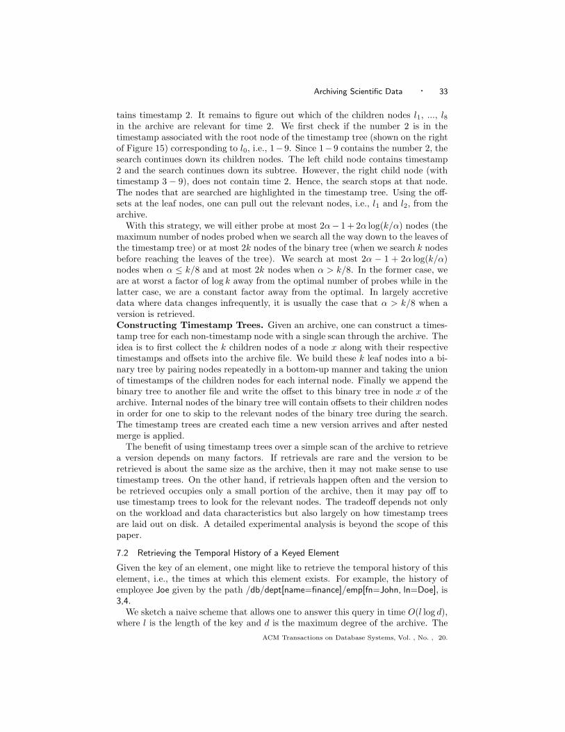
Archiving Scientific Data · 33
tains timestamp 2. It remains to figure out which of the children nodes l1, ..., l8in the archive are relevant for time 2. We first check if the number 2 is in thetimestamp associated with the root node of the timestamp tree (shown on the rightof Figure 15) corresponding to l0, i.e., 1−9. Since 1−9 contains the number 2, thesearch continues down its children nodes. The left child node contains timestamp2 and the search continues down its subtree. However, the right child node (withtimestamp 3 − 9), does not contain time 2. Hence, the search stops at that node.The nodes that are searched are highlighted in the timestamp tree. Using the off-sets at the leaf nodes, one can pull out the relevant nodes, i.e., l1 and l2, from thearchive.
With this strategy, we will either probe at most 2α− 1 + 2α log(k/α) nodes (themaximum number of nodes probed when we search all the way down to the leaves ofthe timestamp tree) or at most 2k nodes of the binary tree (when we search k nodesbefore reaching the leaves of the tree). We search at most 2α − 1 + 2α log(k/α)nodes when α ≤ k/8 and at most 2k nodes when α > k/8. In the former case, weare at worst a factor of log k away from the optimal number of probes while in thelatter case, we are a constant factor away from the optimal. In largely accretivedata where data changes infrequently, it is usually the case that α > k/8 when aversion is retrieved.Constructing Timestamp Trees. Given an archive, one can construct a times-tamp tree for each non-timestamp node with a single scan through the archive. Theidea is to first collect the k children nodes of a node x along with their respectivetimestamps and offsets into the archive file. We build these k leaf nodes into a bi-nary tree by pairing nodes repeatedly in a bottom-up manner and taking the unionof timestamps of the children nodes for each internal node. Finally we append thebinary tree to another file and write the offset to this binary tree in node x of thearchive. Internal nodes of the binary tree will contain offsets to their children nodesin order for one to skip to the relevant nodes of the binary tree during the search.The timestamp trees are created each time a new version arrives and after nestedmerge is applied.
The benefit of using timestamp trees over a simple scan of the archive to retrievea version depends on many factors. If retrievals are rare and the version to beretrieved is about the same size as the archive, then it may not make sense to usetimestamp trees. On the other hand, if retrievals happen often and the version tobe retrieved occupies only a small portion of the archive, then it may pay off touse timestamp trees to look for the relevant nodes. The tradeoff depends not onlyon the workload and data characteristics but also largely on how timestamp treesare laid out on disk. A detailed experimental analysis is beyond the scope of thispaper.
7.2 Retrieving the Temporal History of a Keyed Element
Given the key of an element, one might like to retrieve the temporal history of thiselement, i.e., the times at which this element exists. For example, the history ofemployee Joe given by the path /db/dept[name=finance]/emp[fn=John, ln=Doe], is3,4.
We sketch a naive scheme that allows one to answer this query in time O(l log d),where l is the length of the key and d is the maximum degree of the archive. The
ACM Transactions on Database Systems, Vol. , No. , 20.

34 · Buneman, Khanna, Tajima, and Tan
idea is to maintain, for each keyed node in the archive, a sorted list of key valuesof children nodes. Each node in the sorted list contains its key value, an offset toits sorted list of children nodes (index offset), and an offset to the timestamp nodein the archive in which its timestamps are inherited from (timestamp offset). Weassume that these information are kept in fix size records.
Using the example archive from Figure 4, there is a sorted list of children nodes,dept[name=finance] and dept[name=marketing] for the node db. There is also asorted list emp[fn=Jane,ln=Smith], emp[fn=John,ln=Doe] for node dept[name=finance]and so on. To retrieve the temporal history of the element/db/dept[name=finance]/emp[fn=John, ln=Doe], we first use the sorted list of thedb node. A binary search for the node dept[name=finance] is performed on the list.The index offset in the record dept[name=finance] will lead us to the second sortedlist. A binary search for John Doe is then performed on the second list and thetimestamp offset in the record of will lead us to the desired temporal history.
It is easy to see that to retrieve the temporal history of an element given by apath, one performs a binary search for every key along the path. If a key alongthe path is not found in the sorted list, the required element does not exist in thearchive. Otherwise, we locate the next index list and repeat our binary search. Atthe end, we use the timestamp offset in the record of the desired element to locatethe timestamp node in the archive. The process therefore takes O(l log d) time. Ifa node has a large number of children nodes, one can also consider building moresophisticated index structures, such as a B+ tree, for these children nodes.
The sorted lists can be constructed with a single scan through the archive. Theidea is to first collect the key values of all children nodes of each keyed node as wescan through the archive, keeping track of the timestamp offsets as we go along.All key values of children nodes of any node x are known by the time x is exited.The key values are then sorted and the offset to this sorted list can be written asthe index offset in the record corresponding to node x.
Like timestamp trees, the benefit of using an index over a simple scan of thearchive to retrieve the temporal history of a keyed element depends on many factors.If retrievals are rare and the archive is small, then it may not make sense to createor use an index. On the other hand, if retrievals happen often and the archive ishuge, then it may pay off to use the index to pinpoint the desired node quickly. Adetailed experimental analysis is beyond the scope of this paper.
8. RELATED WORK
There has been considerable research on version management systems for hierar-chical data recently [Marian et al. 2001; Chien et al. 2001; Chawathe et al. 1998].Xyleme system [Marian et al. 2001] takes the sequence-of-delta approach. Theystore the latest version together with all forward completed deltas – changes be-tween successive versions that can also allow one to get to an earlier version byinverting deltas on the latest version. Additional information has to be kept inorder for deltas to be invertible. Another approach taken by Chien et al. [Chienet al. 2001] is a reference-based versioning scheme. The first version is always fullystored. As subsequent versions arrive in the form of updates describing the changes,only newly inserted objects in the latest version are stored. Objects that remain
ACM Transactions on Database Systems, Vol. , No. , 20.

Archiving Scientific Data · 35
unchanged are stored as references to the corresponding object in the previous ver-sion. It is shown that this approach provides good support for (temporal) queriessince it preserves the logical structure of every version as opposed to diff-scripts.Moreover, a usefulness-based storage scheme is shown to give good storage cost andsupports efficient reconstruction of any past version. An earlier versioning schemeproposed by Chawathe et al. [Chawathe et al. 1998] stores updates as annotationson nodes and edges of a graph in the DOEM model as edits are made. A special-ized query language Chorel where annotations can be queried is used to query suchchanges.
There has been substantial work on diff-based approaches for tree-like struc-tures [Tai 1979; Zhang and Shasha 1989; 1990; Chawathe et al. 1996; Chawatheand Garcia-Molina 1997; Cobena et al. 2001]. The general problem of finding theminimum cost edit distance between two ordered trees was first studied by [Tai1979] and subsequently improved by Zhang et al. [Zhang and Shasha 1989; 1990].Chawathe et al. [Chawathe et al. 1996] made further restrictions to obtain a fasteralgorithm for the minimum cost edit distance. A heuristic change detection algo-rithm for unordered trees is also proposed by [Chawathe and Garcia-Molina 1997]with a richer set of edit operations. Another diff technique is proposed by [Cobenaet al. 2001] that uses signatures to find matchings and another top down phaseto compute further matchings heuristically. An external memory algorithm forcomputing minimum-cost edit script for two ordered trees has has been proposedby [Chawathe 1999]. Recently, the use of keys in computing diffs has also beenproposed by DeltaXML [Fontaine 2001] as a more systematic way for identifyingcorresponding elements between two XML versions. In DeltaXML, if some ele-ment has a special attribute key (in their namespace), the system uses the valueof key attribute for identifying corresponding elements in different versions. Thekey attribute and its value has to be created manually or automatically, e.g. byusing XSL. Moreover since key values must “fit” into the unary attribute key, itsuffers from the same problems as ID attributes of XML standard in expressingcomposite keys. Software configuration management systems such as CVS [CVS ]use diff-based techniques that store the last version together with backward deltasbased on line-diffs [Miller and Myers 1985; Myers 1986]. Our archiving system ismore like the Source Code Control System (SCCS) [Rochkind 1975], where the(non-)existence of lines of text at various versions are indicated with timestamps.In SCCS, a line-diff is performed between the incoming version and the latest ver-sion in the repository to determine the forward delta (deletions and insertions only)from the latest version to the new version. The repository file is then updated ac-cording to the delta. A single scan through this repository file retrieves any version.However, changes are not grouped by identical lines. If the same line is repeatedlyinserted and deleted over time, the repository file will contain a series of identicallines marked as deleted and inserted. With keys, our archive will only contain theline once and we use timestamps to mark the existence of the lines at the varioustimes. Nested Merge bears a resemblance to the deep union operator introducedby [Buneman et al. 1999] in that it is conceptually taking a union of two deter-ministic trees. It is also similar to the Merge Template of [Tufte and Maier 2001]that merges two XML documents according to a specified template. The template
ACM Transactions on Database Systems, Vol. , No. , 20.

36 · Buneman, Khanna, Tajima, and Tan
specifies which elements can be merged together, inserted or replaced.
Our work is largely inspired by the work of Driscoll et al. [Driscoll et al. 1989]who studied methods for making data structures persistent. A data structure ispartially persistent if it supports updates to the latest version and access to pastversions. Linked structures where each node is assumed to hold a set of field nameand value pairs can be made partially persistent by the fat node method. Each nodeholds a timestamp of when it is first created and field values within “inherit” thistimestamp. Whenever a field value within a node is modified, the new value alongwith its field name and the current timestamp are added to the node. An accessto version i of field f is done by finding among the values of f , the value withthe largest timestamp less than i. Our data structure is that of a key-annotatedtree where each node has a label and outgoing nodes contain distinct labels due tokeys. One can view the set of child labels of a node as a set of field names in the fatnode. However in our case, each field value can be yet another set of field names,and so on. Another difference concerns updates. Driscoll et al. [Driscoll et al. 1989]assumes the updates to the latest version are known and hence one is not requiredto compute the diff. In our case as well as others [Chawathe et al. 1996; Chawatheand Garcia-Molina 1997; Marian et al. 2001; Cobena et al. 2001], the input isyet another version and hence one is required to compute the correspondences (ordifference). One can certainly apply updates to the latest version directly on thearchive if known.
Our technique differs from existing versioning schemes in the several ways. First,elements in every version are identified by key. A key for an element gives a mean-ingful identifier to the element and is naturally persistent as opposed to generatedobject identifiers. With such persistent identifiers, one can easily detect identicalelements across versions, thus arriving at meaningful change descriptions. Diff tech-niques are based on minimizing edit costs which may give semantically meaninglessdeltas as seen by the Person(Name, BirthDate, Address, Zip) example in Figure 1 ofSection 1. Second, the sequence-of-delta techniques store many deltas separately.Apart from the ability to quickly answer queries about the difference between twosuccessive versions, sequence-of-delta approaches do not immediately lend them-selves to support other (temporal) queries such as the evolutionary history of anelement during a specified time period. Third, although the work by [Chien et al.2001] supports temporal queries to some extent through special procedures tied totheir storage scheme and Chawathe et al. [Chawathe et al. 1998] supports tem-poral queries through a specialized query language, they assume that edits thatgenerate each new version are available. In some cases, edits are not always avail-able. Although OMIM and Swiss-Prot publish update logs tracking new entries andentries that have been modified since the last version, they do not publish exactchanges made to each modified entry. It is also not clear whether they keep trackof these changes. Our technique does not assume the existence of edit scripts andstill makes it easy to discover the evolutionary history of any element. Moreover,since our archive is in XML, existing XML query languages such as XQuery [W3C2001b] can be used to query such documents. It is also mentioned by [Chien et al.2001] that the ideal solution is to represent the history of a versioned document asyet another XML document, for such representation will leverage on web-browsers,
ACM Transactions on Database Systems, Vol. , No. , 20.

Archiving Scientific Data · 37
style sheets, query processors and other tools that already support XML.Most work on temporal databases are in the relational context [Torp et al. 2000].
Every tuple has a timestamp that indicates the period of time that tuple exists. Ifa non-key attribute of some existing tuple is modified, a new tuple with the currenttimestamp is created. The new tuple has the same values on all attributes of thetuple whose values are unmodified and contains the new value only on the attributewhose value has been changed. In contrast, our approach pushes timestamps as fardown the hierarchy as possible. Therefore, only the new attribute value togetherwith its timestamp need to be added to the archive. As a result, it would be morespace-efficient to use our archiving technique for keeping a relational database thatundergoes many changes than to rely on a temporal relational database system forarchiving.
9. CONCLUSIONS AND OPEN ISSUES
We have described a novel approach to archiving data based on naturally occurringkeys. Perhaps the most contrasting difference with traditional approaches is thattraditional diff-based approaches are based on minimizing edit distance and mayignore the historical continuity of elements through time. On the other hand, ourtechnique is “aware” of semantic continuity of elements and therefore, we are ableto describe the temporal history of these elements easily. We have shown thatsuch benefit can be achieved without incurring significant space overhead whencompared with delta-based repositories in our experiments with real scientific dataas well as synthetic data. Moreover, it interacts well with existing compressiontechniques. For example, the OMIM and Swiss-Prot archives are always within 1%and 8% of the sizes of their respective diff repositories and the compressed archivesare always smaller than their respective compressed diff repositories. We have alsodescribed how we can extend our archiving tool to an external memory archiver.
We have detailed analysis of the space performance of our archive compared withother approaches. A detailed performance analysis of the external memory archiver,the space efficiency of the proposed indexing schemes as well as actual performanceof answering various queries using the proposed indexing schemes, however, have yetbeen conducted. Another dimension of analysis would be to conduct experiments,for different change ratios and different query workloads, to find out how our archivewould perform when compared with delta-based repositories where checkpointingmay occur periodically: In the case of our archive, a fresh archive may be createdat every kth addition and in the case of a delta-based repository, an entire versionof data is stored as a whole for every kth version for some constant k. Our archiverassumes the keys for the data are provided by experts of the database. A naturalquestion is whether the keys can be automatically derived, through data analysisor mining methodologies on various versions. There is also the question on whetherwe could relax the various requirements we currently impose on keys. Another issueinvolves changing key structures (or changing schemas); Currently, our archivingtechnique requires that all versions of the database must conform to the same keystructure. Since schemas tend to change slightly over time, a natural question ishow this technique can be extended to archive data under circumstances where thekey structure may also change.
ACM Transactions on Database Systems, Vol. , No. , 20.

38 · Buneman, Khanna, Tajima, and Tan
10. ACKNOWLEDGEMENTS
The authors are grateful to the anonymous reviewers for many useful comments.Peter Buneman is formerly of the University of Pennsylvania and was supportedby NSF IIS 99-77408, NSF DL-2 IIS 98-177408 and a Royal Society Wolfson MeritAward. Sanjeev Khanna is supported by an Alfred P. Sloan Fellowship and by NSFCareer Award CCR-0093117. Part of this work was done while Keishi Tajima wasvisiting University of Pennsylvania. Part of this work was done while Wang-ChiewTan was a Ph.D. student at University of Pennsylvania and was supported by NSFIIS 99-77408 and NSF DL-2 IIS 98-177408.
REFERENCES
Altinel, M. and Franklin, M. J. 2000. Efficient Filtering of XML Documents for SelectiveDissemination of Information. In Proceedings of the International Conference on Very LargeData Bases (VLDB). Cairo, Egypt, 53–64.
Avilla-Campillo, I., Green, T. J., Gupta, A., Onizuka, M., Raven, D., and Suciu, D. 2002.XMLTK: An XML Toolkit for Scalable XML Stream Processing. In Proceedings of PLAN-X:Programming Language Technologies for XML. Pittsburg, Pennsylvania.
Bairoch, A. and Apweiler, R. 2000. The SWISS-PROT protein sequence database and itssupplement TrEMBL. Nucleic Acids Research 28, 45–48.
Buneman, P., Davidson, S., Fan, W., Hara, C., and Tan, W. 2001. Keys for XML. InProceedings of the International World Wide Web Conference(WWW10). Hong Kong, China,201–210.
Buneman, P., Deutsch, A., and Tan, W. 1999. A Deterministic Model for SemistructuredData. In Workshop on Query Processing for Semistructured Data and Non-standard DataFormats. Jerusalem, Israel, 14–19.
CELLBIODBS. The WWW Virtual Library of Cell Biology.http://vlib.org/Science/Cell Biology/databases.shtml.
Chawathe, S. S. 1999. Comparing Hierarchical Data in External Memory. In Proceedings of theInternational Conference on Very Large Data Bases (VLDB). Edinburg, Scotland, 90–101.
Chawathe, S. S., Abiteboul, S., and Widom, J. 1998. Representing and Querying Changes inSemistructured Data. In Proceedings of the International Conference on Data Engineering(ICDE). Orlando, Florida, 4–13.
Chawathe, S. S. and Garcia-Molina, H. 1997. Meaningful Change Detection in StructuredData. In Proceedings of the ACM SIGMOD International Conference on Management ofData (SIGMOD). Tucson, Arizona, 26–37.
Chawathe, S. S., Rajaraman, A., Garcia-Molina, H., and Widom, J. 1996. ChangeDetection in Hierarchically Structured Information. In Proceedings of the ACM SIGMODInternational Conference on Management of Data (SIGMOD). Montreal, Canada, 493–504.
Chien, S., Tsotras, V., and Zaniolo, C. 2001. Efficient Management of MultiversionDocuments by Object Referencing. In Proceedings of the International Conference on VeryLarge Data Bases (VLDB). Roma, Italy, 291–300.
Cobena, G., Abiteboul, S., and Marian, A. 2001. Detecting Changes in XML Documents. InProceedings of the International Conference on Data Engineering (ICDE). Heidelberg,Germany.
CVS. Concurrent Versions System: The open standard for version control.http://www.cvshome.org.
Diao, Y., Fischer, P., Franklin, M. J., and To, R. 2002. Efficient and Scalable Filtering ofXML Documents. In Proceedings of the International Conference on Data Engineering(ICDE). San Jose, California.
Driscoll, J. R., Sarnak, N., Sleator, D. D., and Tarjan, R. E. 1989. Making DataStructures Persistent. Journal of Computer and System Sciences 38, 1, 86–124.
ACM Transactions on Database Systems, Vol. , No. , 20.
Archiving Scientific Data · 39
EMBL-EBI (European Bioinformations Institute). SPTr-XML Documentation.
http://www.ebi.ac.uk/swissprot/SP-ML/.
Fontaine, R. L. 2001. A Delta Format for XML: Identifying Changes in XML Files andRepresenting the Changes in XML. In XML Europe. Berlin, West Germany.
Liefke, H. and Suciu, D. 2000. XMill: an Efficient Compressor for XML Data. In Proceedingsof the ACM SIGMOD International Conference on Management of Data (SIGMOD). Dallas,Texas, 153–164.
Marian, A., Abiteboul, S., Cobena, G., and Mignet, L. 2001. Change-Centric Managementof Versions in an XML Warehouse. In Proceedings of the International Conference on VeryLarge Data Bases (VLDB). Roma, Italy, 581–590.
Maruyama, H., Tamura, K., and Uramoto, N. 2000. Digest Values for DOM (DOMHASH).http://www.trl.ibm.com/projects/xml/xss4j/docs/rfc2803.html.
Miller, W. and Myers, E. 1985. A file comparison program. Software-Practice andExperience 15, 11, 1025–1040.
Motwani, R. and Raghavan, P. 1995. Randomized Algorithms. Cambridge University Press.
Myers, E. 1986. An O(ND) difference algorithm and its variations. Algorithmica 1, 2, 251–266.
OMIM 2000. Online Mendelian Inheritance in Man, OMIM (TM).http://www.ncbi.nlm.nih.gov/omim/.
PDOM. GMD-IPSI XQL Engine Version 1.0.2. http://xml.darmstadt.gmd.de/xql/index.html.
PHYSICSCONSTANTS. The NIST Reference on Constants, Units, and Uncertainty.http://physics.nist.gov/cuu/Constants/links.html.
Ramakrishnan, R. and Gehrke, J. 2002. Database Management Systems. McGraw-HillHigher Education, 3rd Edition.
Rochkind, M. 1975. The Source Code Control System. IEEE Transactions on SoftwareEngineering 1, 4, 364–370.
Schmidt, A. R., Waas, F., Kersten, M. L., Carey, M. J., Manolescu, I., and Busse, R.2002. XMark: A Benchmark for XML Data Management. In Proceedings of the InternationalConference on Very Large Data Bases (VLDB). Hong Kong, China, 974–985.
Tai, K. C. 1979. The tree-to-tree correction problem. Journal of the ACM (JACM) 26, 422–433.
Torp, K., Jensen, C. S., and Snodgrass, R. T. 2000. Effective Timestamping in Databases.The VLDB Journal 8, 3-4, 267–288.
Tufte, K. and Maier, D. 2001. Aggregation and Accumulation of XML Data. IEEE DataEngineering Bulletin 24, 2, 34–39.
W3C. 1998. Extensible markup language (xml) 1.0. http://www.w3.org/TR/REC-xml.
W3C. 1999a. Namespaces in XML. http://www.w3.org/TR/REC-xml-names.
W3C. 1999b. XML Path Language (XPath). http://www.w3.org/TR/xpath.
W3C. 2000. XML Schema Part 1: Structures. http://www.w3.org/TR/xmlschema-1/.
W3C. 2001a. Canonical XML Version 1.0. http://www.w3.org/TR/xml-c14n.
W3C. 2001b. XQuery 1.0: An XML Query Language. http://www.w3.org/TR/xquery/.
XMLTREEDIFF. XML TreeDiff. http://www.alphaworks.ibm.com/formula/xmltreediff.
Zhang, K. and Shasha, D. 1989. Simple fast algorithms for the editing distance between treesand related problems. SIAM Journal of Computing 18, 6, 1245–1262.
Zhang, K. and Shasha, D. 1990. Fast algorithms for unit cost editing distance between trees.Journal of Algorithms 11, 6, 581–621.
Received September 2002; revised March 2003; accepted;
ACM Transactions on Database Systems, Vol. , No. , 20.

40 · Buneman, Khanna, Tajima, and Tan
APPENDIX
A. KEYS FOR XML
Various forms of key specification have been proposed for XML, for example, inXML standard [W3C 1998] and XML Schema [W3C 2000]. We use the system ofkey specification developed in [Buneman et al. 2001] mainly because it provides asimple method for specifying relative keys. Relative keys allow one to define keysin a specified scope and hence one can define a hierarchical set of keys, some ofwhich are relative to others. Here, we briefly review the concept of keys developedin [Buneman et al. 2001].
A.1 XML Model
We model an XML document as a tree whose nodes can be one of the three types:(1) E-node: An E-node is labeled with a tag name, (2) A-node: An A-node is apair consisting of an attribute name and value, and (3) T-node: A T-node consistsof text values only. Only E-nodes can be internal nodes.
A.2 Path Expression
A path expression is a sequence of node names — tag or attribute names. For thepurpose of this paper, we consider only the simple fragment of the path languagediscussed in [Buneman et al. 2001]. The path language consists of the following:(1) the empty path “ε”, (2) a node name, and (3) the concatenation of paths P/Qwhere P and Q are paths defined by these rules. We use “/” as the pathconcatenator just as XPath [W3C 1999b] uses it as a location step separator. InXPath, “/” alone or at the beginning of an XPath expression selects an elementabove the document root. We disallow concatenations where Q begins with “/”.
A.3 Value Equality
The value of a T-node is its data value. The value of an A-node is a pair consistingof its attribute name and its attribute value. The value of an E-node consists ofits tag name and two things: (1) a possibly empty list of values of its E and Tchildren nodes according to the document order, and (2) a possibly empty set ofvalues of its A children nodes. Two nodes are value equal if they agree on theirvalue, i.e., the trees rooted at the nodes are isomorphic by an isomorphism that isidentity on string values according to the type of E-nodes and A-nodes as defined.Finally, we use the notation n1 =v n2 to denote the XML value rooted at node n1
is value equal to the XML value rooted at node n2.
A.4 Keys
A key is a pair (Q, {P1, ..., Pk}) where Q and Pi, i ∈ [1, k] are path expressions. Qis the target path and Pi are the key paths. Informally, Q identifies a set of nodes –target set – reachable from some context node and the target set satisfies the keyconstraints given by the key paths. This is analogous to relational database whereQ is a relation name and Pis form the key for that relation. A formal definition isgiven below. We denote by n[[P ]] the set of nodes reachable from node n via pathP .Definition. A node n satisfies a key specification (Q, {P1, . . . , Pk}) if
ACM Transactions on Database Systems, Vol. , No. , 20.

Archiving Scientific Data · 41
—For every n′ in n[[Q]] and for each Pi, (1 ≤ i ≤ k), Pi is unique at n′.
—For any n1, n2 in n[[Q]], if n1[[Pi]] =v n2[[Pi]], (1 ≤ i ≤ k), then n1 = n2.
In the definition above, =v denotes value equality and = denotes node equality(whether two nodes are the exact same node). This is the definition of strong keysgiven in [Buneman et al. 2001].Example. The document below does not satisfy the key (/DB/A, {B}) since bothA elements have the same key path value, i.e., <B> 1 </B>. However, thedocument satisfies the key (/DB/A, {C}). Observe that these keys are specifiedwith respect to the root of the document.
<DB> <A><B> 1 </B><C> 1 </C></A> <A><B> 1 </B><C> 2 </C></A> </DB>
A.5 Relative Keys
Keys as discussed above are defined with respect to some node. We often wouldlike to describe the key of some node dependent on the key of an ancestor nodemuch like weak entities in relational databases [Ramakrishnan and Gehrke 2002].For example, the key of a weak entity consists of its parent’s key and its key (e.g.,course Math120, section B). Such dependent keys can be expressed throughrelative keys as defined below.Definition. A document satisfies a relative key (Q, (Q′, S)) if for all nodes n in[[Q]], n satisfies the key (Q′, S).The target path Q′ identifies the target set relative to the context path Q and Q isalways defined with respect to the document root. In other words, “/” is always aprefix of Q. In this paper, we use the word key to mean a relative key.Example. An example of a set of relative keys can be found in the keys for thecompany database in Example 2. Versions 1 to 4 of Figure 2 are examples ofdatabases that satisfy these keys.
A.6 Value Inequality
A node n1 is less than or equal to a node n2, denoted as n1 ≤v n2, if n1 <v n2 orn1 =v n2. The nodes n1 <v n2 if
—n1 is a T-node, n2 is not a T-node, or
—n1 is an A-node, n2 is an E-node, or
—n1 and n2 are both T-nodes and text(n1) < text(n2) where text(n) denotes thetext string associated with T-node n,
—n1 and n2 are both A-nodes and (i) l1 < l2, or (ii) l1 = l2 and v1 < v2 where(l1, v1) and (l2, v2) are the pairs of attribute name and value associated withnodes n1 and n2 respectively, or
—n1 and n2 are both E-nodes and (i) tag(n1) < tag(n2), or (ii) tag(n1) = tag(n2)and children(n1) <l children(n2), or (iii) tag(n1) = tag(n2), children(n1) =l
children(n2), and attr(n1) <s attr(n2). Next, we define ≤l and ≤s.Let children(n1) be [c1, ..., cm] and children(n2) be [c′1, ..., c
′
n] where each childnode is either a T or E-node. Then, [c1, ..., cm] <l [c′1, ..., c
′
n] if
—m < n, or—m = n and ci =v c′i for all i ∈ [1, k − 1], k ∈ [1, m], and ck <v c′k.
ACM Transactions on Database Systems, Vol. , No. , 20.

42 · Buneman, Khanna, Tajima, and Tan
We have [c1, ..., cm] =l [c′1, ..., c′
n] if m = n and ci =v c′i for all i ∈ [1, m].
Let attr(n1) and attr(n2) be {l1 = v1, ..., lm = vm} and {l′1 = v′1, ..., l′
n = v′n}respectively where lis and l′is are lexicographically ordered. Then,{l1 = v1, ..., lm = vm} <s {l′1 = v′1, ..., l
′
n = v′n} if—m < n, or—m = n, li = l′i, vi = v′i for i ∈ [1, k − 1], k ∈ [1, m], lk < l′k, or—m = n, li = l′i, vi = v′i for i ∈ [1, k − 1], k ∈ [1, m], lk = l′k, and vk < v′k.We have {l1 = v1, ..., lm = vm} =s {l′1 = v′1, ..., l
′
n = v′n} if m = n, li = l′i, vi = v′ifor i ∈ [1, m].
ACM Transactions on Database Systems, Vol. , No. , 20.

Archiving Scientific Data · 43
B. SAMPLE DATA
B.1 Sample record and keys from OMIM
A sample OMIM record is shown below. Some fields of OMIM have been omittedduring our translation into XML because they appear in inconsistent formats inolder versions of OMIM.
<ROOT>
<Record>
<Num>102579</Num>
<Title>*102579 REPLICATION FACTOR C, 140-KD SUBUNIT; RFC1</Title>
<AlternativeTitle>REPLICATION FACTOR C1</AlternativeTitle>
<AlternativeTitle>RFC*FIELD* TX</AlternativeTitle>
<Text>Replication factor C is a multisubunit, ... </Text>
<Contributors>
<Name>Paul J. Converse</Name>
<CNtype>updated</CNtype>
<Date> <Month>11</Month> <Day>16</Day> <Year>2000</Year> </Date>
</Contributors>
<Contributors>
<Name>Jennifer P. Macke</Name>
<CNtype>updated</CNtype>
<Date> <Month>8</Month> <Day>27</Day> <Year>1997</Year> </Date>
</Contributors>
<Creation_Date>
<Name>Victor A. McKusick</Name>
<Date> <Month>12</Month> <Day>14</Day> <Year>1993</Year> </Date>
</Creation_Date>
</Record>
...
</ROOT>
Keys for OMIM data are shown below (many fields in the keys are not reflected inthe above sample record):
(/, (ROOT, {}))
(/ROOT, (Record, {Num}))
(/ROOT/Record, (Title, {}))
(/ROOT/Record, (AlternativeTitle, {\e}))
(/ROOT/Record, (Text, {}))
(/ROOT/Record, (Ref, {\e}))
(/ROOT/Record, (Contributors,
{Name, CNtype, Date/Month, Date/Day, Date/Year}))
(/ROOT/Record/Contributors, (Date, {}))
(/ROOT/Record, (Creation_Date, {Name, Date/Month, Date/Day, Date/Year}))
(/ROOT/Record/Creation_Date, (Date, {}))
(/ROOT/Record, (Edit_History, {Name, Date/Month, Date/Day, Date/Year}))
(/ROOT/Record/Edit_History, (Date, {}))
(/ROOT/Record, (Clinical_Synop, {Part, Synop}))
(/ROOT/Record, (See_Also, {Authors, Year}))
(/ROOT/Record, (Allelic_Variants, {Id}))
(/ROOT/Record/Allelic_Variants, (Name, {}))
ACM Transactions on Database Systems, Vol. , No. , 20.
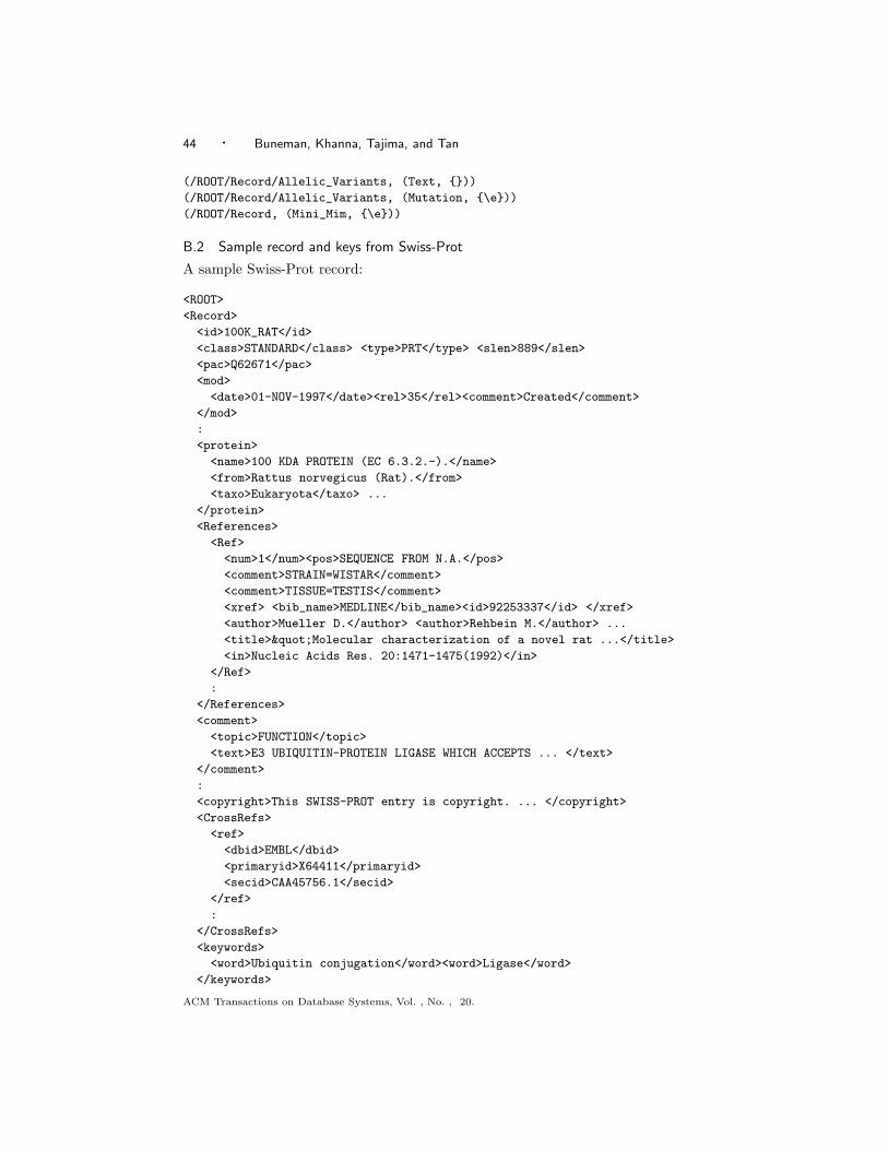
44 · Buneman, Khanna, Tajima, and Tan
(/ROOT/Record/Allelic_Variants, (Text, {}))
(/ROOT/Record/Allelic_Variants, (Mutation, {\e}))
(/ROOT/Record, (Mini_Mim, {\e}))
B.2 Sample record and keys from Swiss-Prot
A sample Swiss-Prot record:
<ROOT>
<Record>
<id>100K_RAT</id>
<class>STANDARD</class> <type>PRT</type> <slen>889</slen>
<pac>Q62671</pac>
<mod>
<date>01-NOV-1997</date><rel>35</rel><comment>Created</comment>
</mod>
:
<protein>
<name>100 KDA PROTEIN (EC 6.3.2.-).</name>
<from>Rattus norvegicus (Rat).</from>
<taxo>Eukaryota</taxo> ...
</protein>
<References>
<Ref>
<num>1</num><pos>SEQUENCE FROM N.A.</pos>
<comment>STRAIN=WISTAR</comment>
<comment>TISSUE=TESTIS</comment>
<xref> <bib_name>MEDLINE</bib_name><id>92253337</id> </xref>
<author>Mueller D.</author> <author>Rehbein M.</author> ...
<title>"Molecular characterization of a novel rat ...</title>
<in>Nucleic Acids Res. 20:1471-1475(1992)</in>
</Ref>
:
</References>
<comment>
<topic>FUNCTION</topic>
<text>E3 UBIQUITIN-PROTEIN LIGASE WHICH ACCEPTS ... </text>
</comment>
:
<copyright>This SWISS-PROT entry is copyright. ... </copyright>
<CrossRefs>
<ref>
<dbid>EMBL</dbid>
<primaryid>X64411</primaryid>
<secid>CAA45756.1</secid>
</ref>
:
</CrossRefs>
<keywords>
<word>Ubiquitin conjugation</word><word>Ligase</word>
</keywords>
ACM Transactions on Database Systems, Vol. , No. , 20.
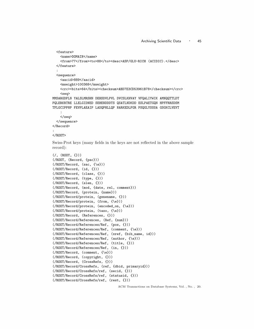
Archiving Scientific Data · 45
<feature>
<name>DOMAIN</name>
<from>77</from><to>88</to><desc>ASP/GLU-RICH (ACIDIC).</desc>
</feature>
:
<sequence>
<aacid>889</aacid>
<mweight>100368</mweight>
<crc><bits>64</bits><checksum>ABD7E3CD53961B78</checksum></crc>
<seq>
MMSARGDFLN YALSLMRSHN DEHSDVLPVL DVCSLKHVAY VFQALIYWIK AMNQQTTLDT
PQLERKRTRE LLELGIDNED SEHENDDDTS QSATLNDKDD ESLPAETGQN HPFFRRSDSM
TFLGCIPPNP FEVPLAEAIP LADQPHLLQP NARKEDLFGR PSQGLYSSSA GSGKCLVEVT
:
</seq>
</sequence>
</Record>
:
</ROOT>
Swiss-Prot keys (many fields in the keys are not reflected in the above samplerecord):
(/, (ROOT, {}))
(/ROOT, (Record, {pac}))
(/ROOT/Record, (sac, {\e}))
(/ROOT/Record, (id, {}))
(/ROOT/Record, (class, {}))
(/ROOT/Record, (type, {}))
(/ROOT/Record, (slen, {}))
(/ROOT/Record, (mod, {date, rel, comment}))
(/ROOT/Record, (protein, {name}))
(/ROOT/Record/protein, (genename, {}))
(/ROOT/Record/protein, (from, {\e}))
(/ROOT/Record/protein, (encoded_on, {\e}))
(/ROOT/Record/protein, (taxo, {\e}))
(/ROOT/Record, (References, {}))
(/ROOT/Record/References, (Ref, {num}))
(/ROOT/Record/References/Ref, (pos, {}))
(/ROOT/Record/References/Ref, (comment, {\e}))
(/ROOT/Record/References/Ref, (xref, {bib_name, id}))
(/ROOT/Record/References/Ref, (author, {\e}))
(/ROOT/Record/References/Ref, (title, {}))
(/ROOT/Record/References/Ref, (in, {}))
(/ROOT/Record, (comment, {\e}))
(/ROOT/Record, (copyright, {}))
(/ROOT/Record, (CrossRefs, {}))
(/ROOT/Record/CrossRefs, (ref, {dbid, primaryid}))
(/ROOT/Record/CrossRefs/ref, (secid, {}))
(/ROOT/Record/CrossRefs/ref, (statusid, {}))
(/ROOT/Record/CrossRefs/ref, (rest, {}))
ACM Transactions on Database Systems, Vol. , No. , 20.
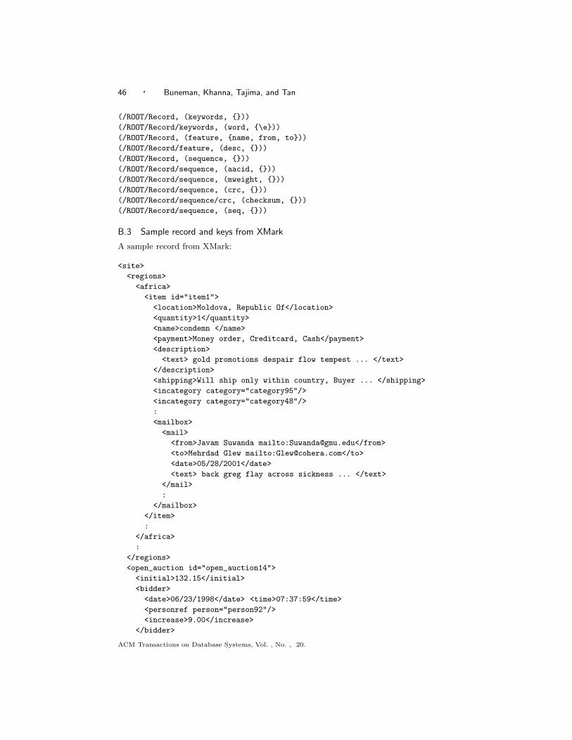
46 · Buneman, Khanna, Tajima, and Tan
(/ROOT/Record, (keywords, {}))
(/ROOT/Record/keywords, (word, {\e}))
(/ROOT/Record, (feature, {name, from, to}))
(/ROOT/Record/feature, (desc, {}))
(/ROOT/Record, (sequence, {}))
(/ROOT/Record/sequence, (aacid, {}))
(/ROOT/Record/sequence, (mweight, {}))
(/ROOT/Record/sequence, (crc, {}))
(/ROOT/Record/sequence/crc, (checksum, {}))
(/ROOT/Record/sequence, (seq, {}))
B.3 Sample record and keys from XMark
A sample record from XMark:
<site>
<regions>
<africa>
<item id="item1">
<location>Moldova, Republic Of</location>
<quantity>1</quantity>
<name>condemn </name>
<payment>Money order, Creditcard, Cash</payment>
<description>
<text> gold promotions despair flow tempest ... </text>
</description>
<shipping>Will ship only within country, Buyer ... </shipping>
<incategory category="category95"/>
<incategory category="category48"/>
:
<mailbox>
<mail>
<from>Javam Suwanda mailto:[email protected]</from>
<to>Mehrdad Glew mailto:[email protected]</to>
<date>05/28/2001</date>
<text> back greg flay across sickness ... </text>
</mail>
:
</mailbox>
</item>
:
</africa>
:
</regions>
<open_auction id="open_auction14">
<initial>132.15</initial>
<bidder>
<date>06/23/1998</date> <time>07:37:59</time>
<personref person="person92"/>
<increase>9.00</increase>
</bidder>
ACM Transactions on Database Systems, Vol. , No. , 20.
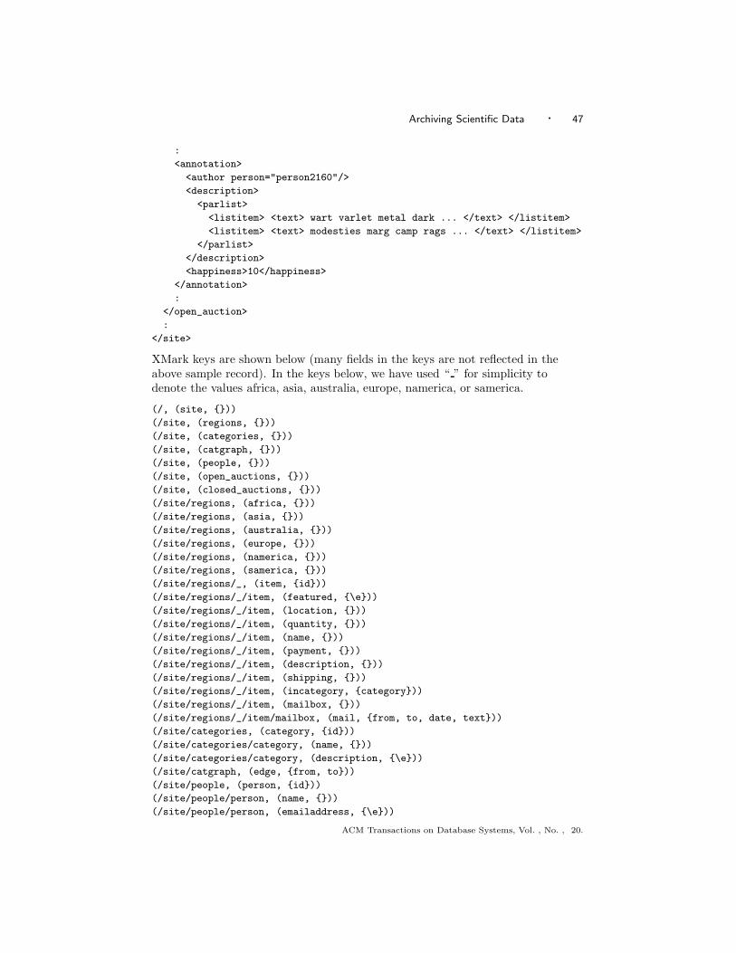
Archiving Scientific Data · 47
:
<annotation>
<author person="person2160"/>
<description>
<parlist>
<listitem> <text> wart varlet metal dark ... </text> </listitem>
<listitem> <text> modesties marg camp rags ... </text> </listitem>
</parlist>
</description>
<happiness>10</happiness>
</annotation>
:
</open_auction>
:
</site>
XMark keys are shown below (many fields in the keys are not reflected in theabove sample record). In the keys below, we have used “ ” for simplicity todenote the values africa, asia, australia, europe, namerica, or samerica.
(/, (site, {}))
(/site, (regions, {}))
(/site, (categories, {}))
(/site, (catgraph, {}))
(/site, (people, {}))
(/site, (open_auctions, {}))
(/site, (closed_auctions, {}))
(/site/regions, (africa, {}))
(/site/regions, (asia, {}))
(/site/regions, (australia, {}))
(/site/regions, (europe, {}))
(/site/regions, (namerica, {}))
(/site/regions, (samerica, {}))
(/site/regions/_, (item, {id}))
(/site/regions/_/item, (featured, {\e}))
(/site/regions/_/item, (location, {}))
(/site/regions/_/item, (quantity, {}))
(/site/regions/_/item, (name, {}))
(/site/regions/_/item, (payment, {}))
(/site/regions/_/item, (description, {}))
(/site/regions/_/item, (shipping, {}))
(/site/regions/_/item, (incategory, {category}))
(/site/regions/_/item, (mailbox, {}))
(/site/regions/_/item/mailbox, (mail, {from, to, date, text}))
(/site/categories, (category, {id}))
(/site/categories/category, (name, {}))
(/site/categories/category, (description, {\e}))
(/site/catgraph, (edge, {from, to}))
(/site/people, (person, {id}))
(/site/people/person, (name, {}))
(/site/people/person, (emailaddress, {\e}))
ACM Transactions on Database Systems, Vol. , No. , 20.

48 · Buneman, Khanna, Tajima, and Tan
(/site/people/person, (phone, {\e}))
(/site/people/person, (address, {\e}))
(/site/people/person, (homepage, {\e}))
(/site/people/person, (creditcard, {\e}))
(/site/people/person, (profile, {\e}))
(/site/people/person, (watches, {\e}))
(/site/open_auctions, (open_auction, {id}))
(/site/open_auctions/open_auction, (initial, {}))
(/site/open_auctions/open_auction, (reserve, {\e}))
(/site/open_auctions/open_auction,
(bidder, {date, time, personref/person, increase}))
(/site/open_auctions/open_auction/bidder, (personref, {}))
(/site/open_auctions/open_auction, (current, {}))
(/site/open_auctions/open_auction, (privacy, {\e}))
(/site/open_auctions/open_auction, (itemref, {}))
(/site/open_auctions/open_auction/itemref, (item, {}))
(/site/open_auctions/open_auction, (seller, {}))
(/site/open_auctions/open_auction/seller, (person, {}))
(/site/open_auctions/open_auction, (annotation, {}))
(/site/open_auctions/open_auction/annotation, (author, {}))
(/site/open_auctions/open_auction/annotation/author, (person, {}))
(/site/open_auctions/open_auction/annotation, (description, {}))
(/site/open_auctions/open_auction/annotation, (happiness, {}))
(/site/open_auctions/open_auction, (quantity, {}))
(/site/open_auctions/open_auction, (type, {}))
(/site/open_auctions/open_auction, (interval, {start,end}))
(/site/closed_auctions,
(closed_auction, {seller, buyer, itemref/item, date}))
(/site/closed_auctions/closed_auction, (itemref, {}))
(/site/closed_auctions/closed_auction, (price, {}))
(/site/closed_auctions/closed_auction, (annotation, {}))
(/site/closed_auctions/closed_auction/annotation, (author, {}))
(/site/closed_auctions/closed_auction/annotation/author, (person, {}))
(/site/closed_auctions/closed_auction/annotation, (description, {}))
(/site/closed_auctions/closed_auction/annotation, (happiness, {}))
(/site/closed_auctions/closed_auction, (quantity, {}))
(/site/closed_auctions/closed_auction, (type, {}))
ACM Transactions on Database Systems, Vol. , No. , 20.

Archiving Scientific Data · 49
C. ADDITIONAL EXPERIMENTAL RESULTS
C.1 Storage performance on XMark under different change ratio
Size (bytes) x 106 Size (bytes) x 106
Auction Data (10)
archiveV1 + incremental diffsversiongzip(V1 + cumulative diffs)xmill(V1+...+Vi)gzip(V1 + incremental diffs)xmill(archive)
size (bytes) x 106
version sequence
0.00
2.00
4.00
6.00
8.00
10.00
12.00
14.00
16.00
18.00
20.00
22.00
24.00
26.00
28.00
30.00
0.00 5.00 10.00 15.00 20.00
PSfrag replacements
a1
a2
am
b1
b2
bn
Original document
Run 1Run 2Run n
Auction Data (20)
archiveV1 + incremental diffsversiongzip(V1 + cumulative diffs)xmill(V1+...+Vi)gzip(V1 + incremental diffs)xmill(archive)
size (bytes) x 106
version sequence
0.00
5.00
10.00
15.00
20.00
25.00
30.00
35.00
40.00
45.00
0.00 5.00 10.00 15.00 20.00
PSfrag replacements
a1
a2
am
b1
b2
bn
Original document
Run 1Run 2Run n
V1+incdiffs
arch
ive
gzip(V
1+
cum
udiff
s)
version
xmill(archive)
xmill(V
1+ ... +
Vi)
gzip(V
1+inc
diffs)
version gzip(V
1+incdiffs
)
xmill(
V1
+...
+V i
)
xmill(
archiv
e)
gzip
(V1+
cum
udiff
s)
arch
iveV1+
inc
diffs
Number of Versions
(a) 3.33%/3.33%/3.33% change ratio (b) 6.66%/6.66%/6.66% change ratio
ACM Transactions on Database Systems, Vol. , No. , 20.

50 · Buneman, Khanna, Tajima, and Tan
C.2 Storage performance on XMark with insertion and deletion of highly similarelements
Size (bytes) x 106 Size (bytes) x 106
Auction Data (10)
archiveV1 + incremental diffsversiongzip(V1 + cumulative diffs)xmill(V1+...+Vi)gzip(V1 + incremental diffs)xmill(archive)
size (bytes) x 106
version sequence
0.00
1.00
2.00
3.00
4.00
5.00
6.00
7.00
8.00
9.00
10.00
11.00
12.00
13.00
14.00
15.00
16.00
17.00
18.00
19.00
20.00
0.00 5.00 10.00 15.00 20.00
PSfrag replacements
a1
a2
am
b1
b2
bn
Original document
Run 1Run 2Run n
Auction Data (20)
archiveV1 + incremental diffsversiongzip(V1 + cumulative diffs)xmill(V1+...+Vi)gzip(V1 + incremental diffs)xmill(archive)
size (bytes) x 106
version sequence
0.00
2.00
4.00
6.00
8.00
10.00
12.00
14.00
16.00
18.00
20.00
22.00
24.00
26.00
28.00
0.00 5.00 10.00 15.00 20.00
PSfrag replacements
a1
a2
am
b1
b2
bn
Original document
Run 1Run 2Run n
V1+inc diffs
arch
ive
gzip(V1+cumu diffs)
version
xmill(archive)
xmill(V1 + ... + Vi) gzip(V1+inc diffs)
version
xmill(archive)
gzip(V1+inc diffs)gzip(V1+inc diffs),
xmill(V1 + ... + Vi)
arch
ive
V1+inc diffs
Number of Versions
(a) 3.33%/3.33%/3.33% change ratio (b) 6.66%/6.66%/6.66% change ratio
ACM Transactions on Database Systems, Vol. , No. , 20.