ARCH Modelling of the Exchange and Interest Rates in - DOFIN

Applications of ARCH modelling in financial time

series: the case of Germany

I. Exchange rate volatility modelling.

II. Time varying-premium in the term structure of interest rates.

Research Techniques Project

Florin Ovidiu Bilbiie May 2000

Department of Economics

University of Warwick

Coventry CV4 7AL

Email: [email protected]

mailto:[email protected]

2

Introduction

ARCH and GARCH models in empirical finance have gained a wide use since their initial

introduction by Engle (1982) to describe different phenomena. Mills (1999) and Bollerslev et al

(1994) contain comprehensive surveys of these developments and of applications. This paper

approaches two topics. In the first part we model the returns for the DEM/USD rate, more

specifically its volatility, by using ARCH and GARCH models. In the second one, we apply the

same tools to model a time-varying term premium in the yield curve that might explain failures of

the expectation hypothesis.

PART 1 -Exchange rate volatility modelling

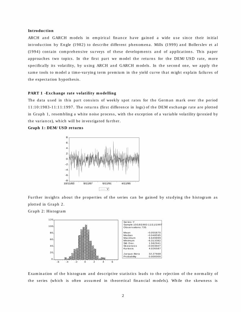
The data used in this part consists of weekly spot rates for the German mark over the period

11:10:1983-11:11:1997. The returns (first difference in logs) of the DEM exchange rate are plotted

in Graph 1, resembling a white noise process, with the exception of a variable volatility (proxied by

the variance), which will be investigated further.

Graph 1: DEM/USD returns

Further insights about the properties of the series can be gained by studying the histogram as

plotted in Graph 2.

Graph 2: Histogram

Examination of the histogram and descriptive statistics leads to the rejection of the normality of

the series (which is often assumed in theoretical financial models). While the skewness is

-8

-6

-4

-2

0

2

4

6

8

10/11/83 8/11/87 6/11/91 4/11/95

Y

0

20

40

60

80

100

120

-6 -4 -2 0 2 4 6

Ser ies : YSample 10/18/1983 11/11/1997Obs erv ations 735

Mean -0.055870Median -0.048595Max imum 6.649899Minimum -6.313382Std. D ev . 1.562941Skew nes s -0.003607Kur tos is 4.026587

J arque-Bera 32.27668Probability 0.000000

3

reasonably small, the excess kurtosis leads to the rejection of normality. This is indicated by the

highly significant Jarque-Berra statistic. More specifically, the distribution is leptokurtic (it has

fat tails), which usually generates a 'volatility smile' in the options on exchange rates (different

implied volatilities for different exercise prices but same other characteristics). This finding is

rather a common result (i.a Diebold and Nerlove (1989)). We also mention that the series is

stationary, the ADF tests we performed rejecting the hypothesis of a unit root at 1% critical level

(not reported, available at request), making subsequent statistical inference valid.

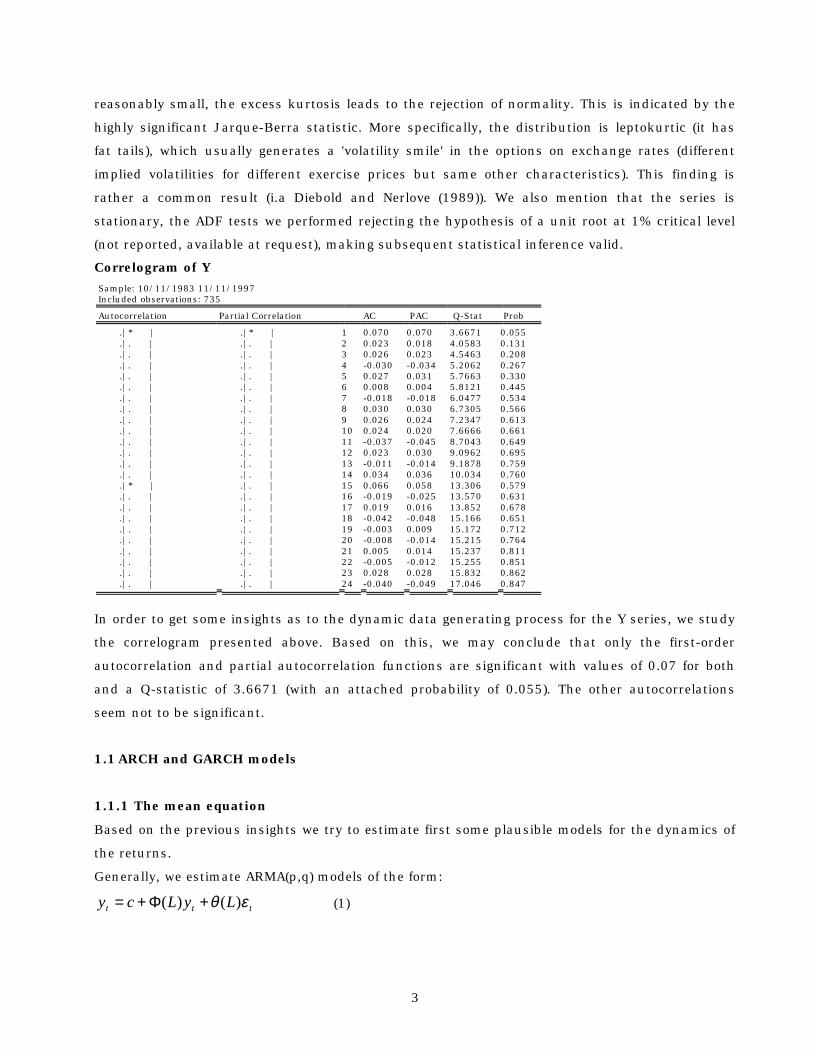
Correlogram of Y Sample: 10/11/1983 11/11/1997 Included observations: 735

Autocorrelation Partial Correlation AC PAC Q-Stat Prob

.|* | .|* | 1 0.070 0.070 3.6671 0.055 .|. | .|. | 2 0.023 0.018 4.0583 0.131 .|. | .|. | 3 0.026 0.023 4.5463 0.208 .|. | .|. | 4 -0.030 -0.034 5.2062 0.267 .|. | .|. | 5 0.027 0.031 5.7663 0.330 .|. | .|. | 6 0.008 0.004 5.8121 0.445 .|. | .|. | 7 -0.018 -0.018 6.0477 0.534 .|. | .|. | 8 0.030 0.030 6.7305 0.566 .|. | .|. | 9 0.026 0.024 7.2347 0.613 .|. | .|. | 10 0.024 0.020 7.6666 0.661 .|. | .|. | 11 -0.037 -0.045 8.7043 0.649 .|. | .|. | 12 0.023 0.030 9.0962 0.695 .|. | .|. | 13 -0.011 -0.014 9.1878 0.759 .|. | .|. | 14 0.034 0.036 10.034 0.760 .|* | .|. | 15 0.066 0.058 13.306 0.579 .|. | .|. | 16 -0.019 -0.025 13.570 0.631 .|. | .|. | 17 0.019 0.016 13.852 0.678 .|. | .|. | 18 -0.042 -0.048 15.166 0.651 .|. | .|. | 19 -0.003 0.009 15.172 0.712 .|. | .|. | 20 -0.008 -0.014 15.215 0.764 .|. | .|. | 21 0.005 0.014 15.237 0.811 .|. | .|. | 22 -0.005 -0.012 15.255 0.851 .|. | .|. | 23 0.028 0.028 15.832 0.862 .|. | .|. | 24 -0.040 -0.049 17.046 0.847

In order to get some insights as to the dynamic data generating process for the Y series, we study

the correlogram presented above. Based on this, we may conclude that only the first-order

autocorrelation and partial autocorrelation functions are significant with values of 0.07 for both

and a Q-statistic of 3.6671 (with an attached probability of 0.055). The other autocorrelations

seem not to be significant.

1.1 ARCH and GARCH models 1.1.1 The mean equation

Based on the previous insights we try to estimate first some plausible models for the dynamics of

the returns.

Generally, we estimate ARMA(p,q) models of the form:

ttt LyLcy εθ )()( +Φ+= (1)

4

where ΦΦΦΦ and θθθθ are lag polynomials of the p and q order respectively, where ΦΦΦΦ does not have a free

term.

As there appears to be informational content only for the first lag (judging by the correlograms),

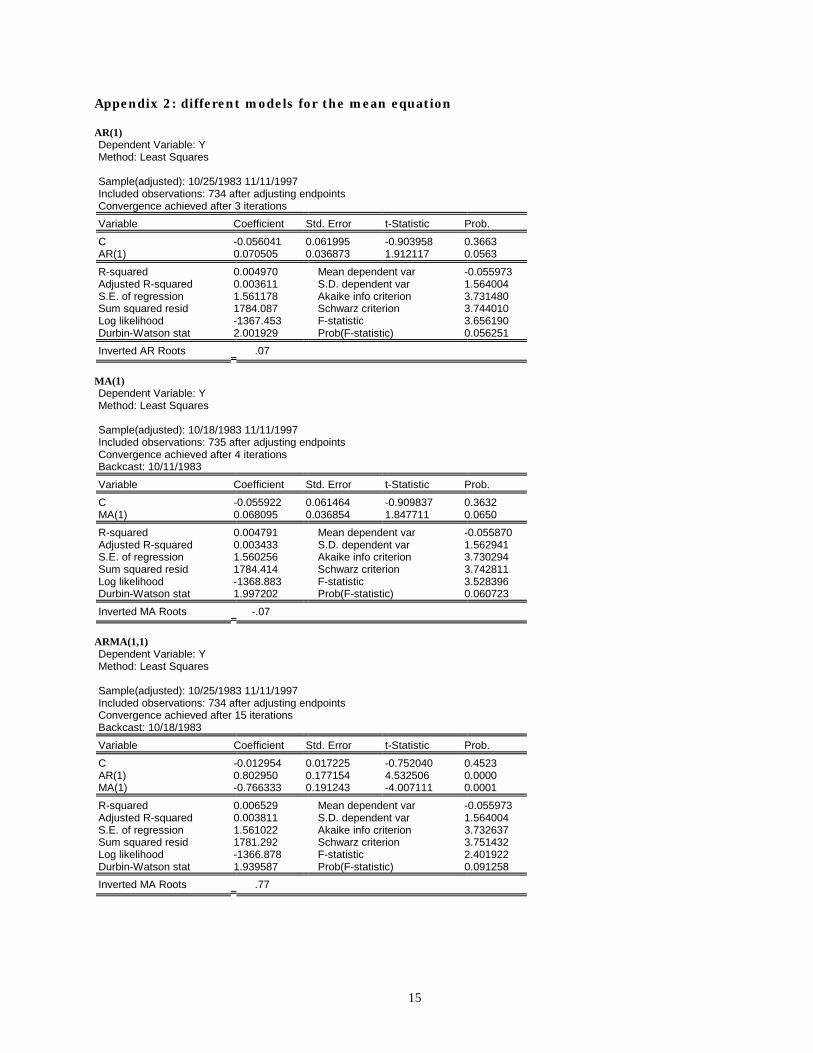
we tried to estimate AR(1), MA(1) and ARMA(1,1) models presenting the outputs in Appendix 21.

Judging by the AIC and the SBC the MA(1) model would seem the most appropriate. On the other

hand, the AR(1) term proves to be significant in the ARMA (1,1) equation. We decided not to use

the ARMA specification, however, due to the common factor that appears to be present. Testing

(by a Wald test) the hypothesis that Φ1=-θ1 we obtained an F Statistic of 1.853856 (0.173755)

leading to a non-rejection of the common factor. This would imply that the mean equation would

comprise only a constant, which would be consistent with the non-predictability of returns (weak

efficiency). However, as there seems to be informational content attached to the first lag (Φ1 is

marginally significant) we use an AR(1) model. This is far easier to manipulate and to use for

forecasts and the improvement in the AIC and SBC are, however, marginal. In terms of the

residual test, all the models perform similarly, so this cannot be a decision rule we rely upon.

Moreover, we find support in Diebold and Nerlove (1989) who use an AR(3) even if they find a

random walk to be the best description, arguing that this is a safeguard against specification

error. This would account for any potential non-captured weakly serial correlation.

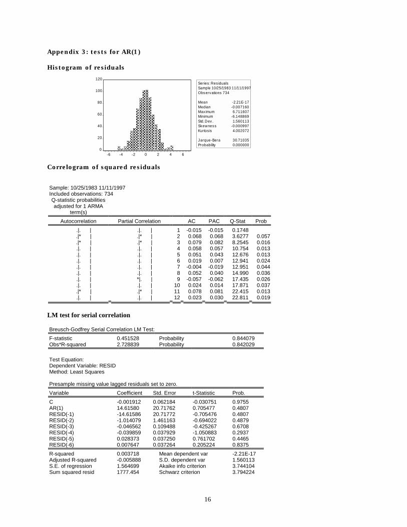
We present some of the residual tests for the chosen AR(1) (but not for the ARMA and MA models)

model in Appendix 3. The Breusch-Godfrey test does not reject the null hypothesis of no serial

correlation (conclusion supported by the plot of the correlogram) with a value of 0.451528 and an

attached probability of 0.844079.

However, there is strong evidence of non-normality as indicated by the Jarque-Berra test (rejects

normality at 0.00000 significance level) and the histogram plot.

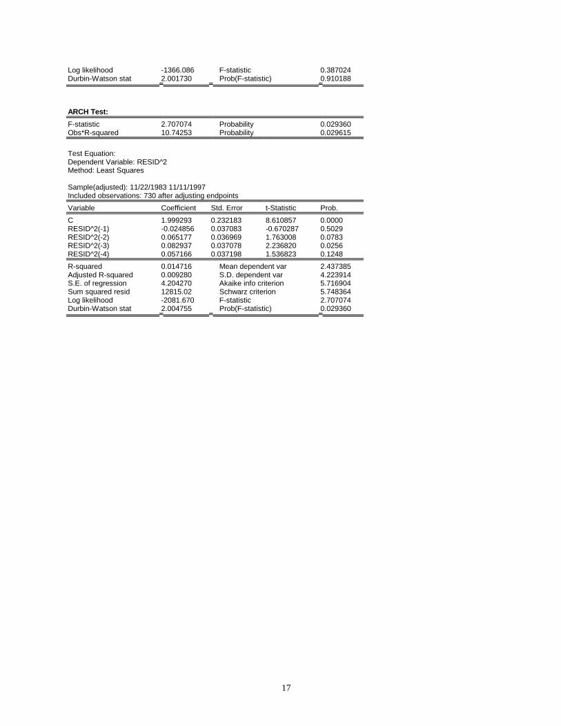
An ARCH LM test indicates strong ARCH effects for the first three lags, consistent with the

conclusion from the correlogram of the squared residuals. Thus the residuals are, although

uncorrelatted, not independent. Finding and modelling ARCH effects help explaining contiguous

periods of volatility and stability. Secondly, they are consistent with the unconditional

leptokurtosis we found in the returns' distribution. Thirdly, they provide a parsimonious

description of the evolving conditional variance. Fourthly, it would help forecasting the changing

variance, i.e. to obtain time-varying confidence intervals for the point forecasts of the returns.

This leads us to the next step, i.e. using ARCH models to explain the changing variance.

I.1.2 Modelling the conditional variance

Following Engle (1982), we estimate the model:

5

),0(~/)(

1

211

ttt

tt

ttt

hNwhereLAh

ycy

−

−

Ω=

+Φ+=

εε

ε

(2)

A(L) is a lag polynomial of order m.

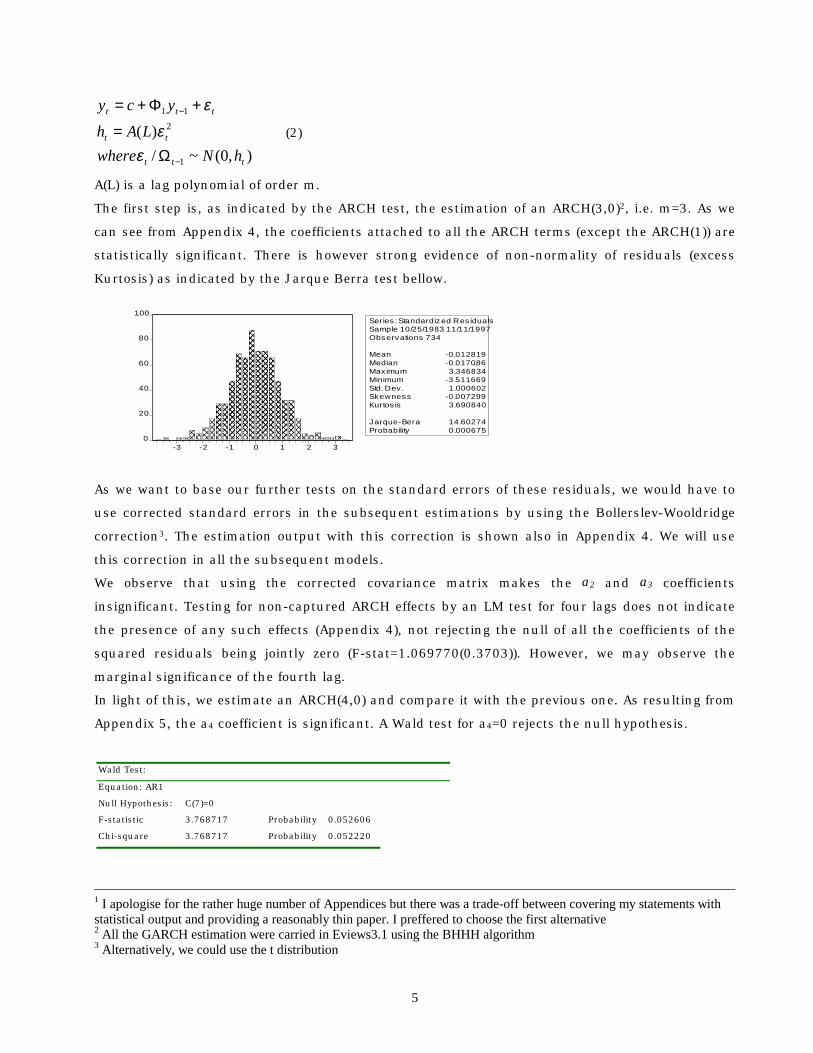
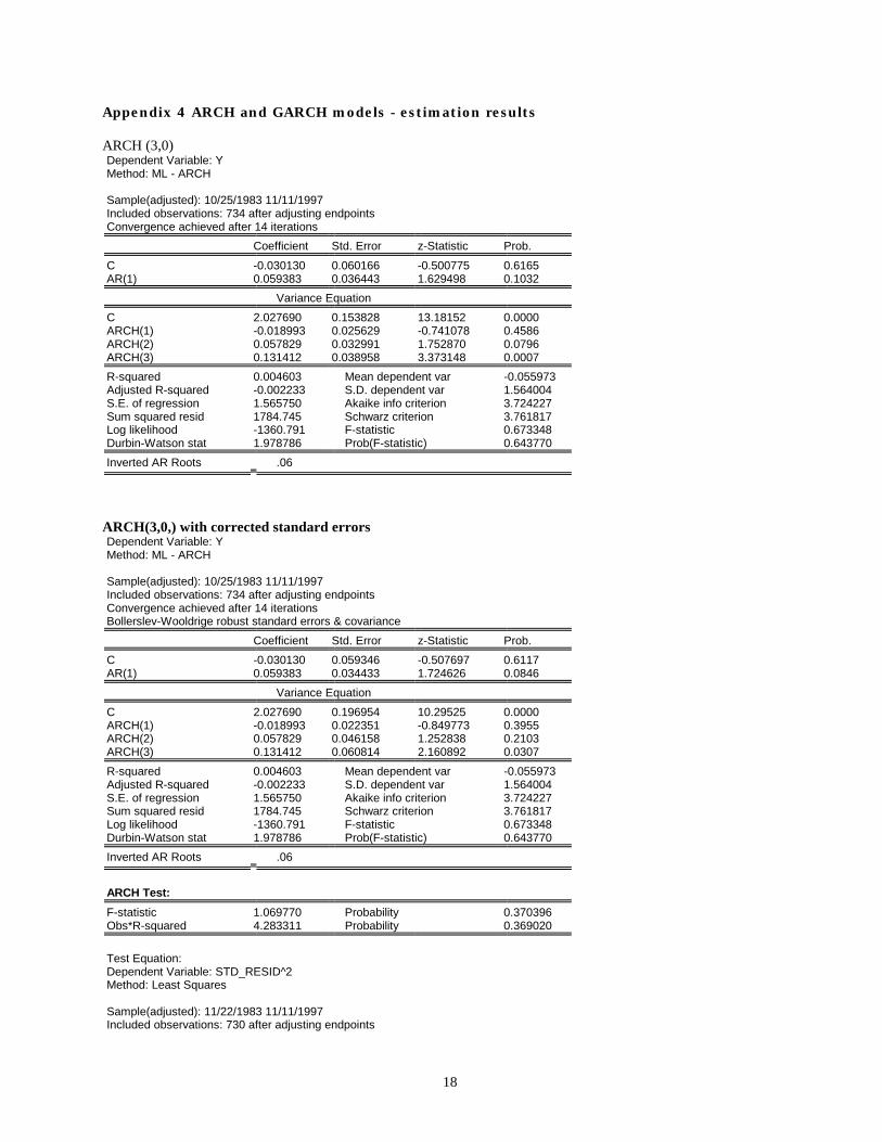
The first step is, as indicated by the ARCH test, the estimation of an ARCH(3,0)2, i.e. m=3. As we

can see from Appendix 4, the coefficients attached to all the ARCH terms (except the ARCH(1)) are

statistically significant. There is however strong evidence of non-normality of residuals (excess

Kurtosis) as indicated by the Jarque Berra test bellow.

As we want to base our further tests on the standard errors of these residuals, we would have to

use corrected standard errors in the subsequent estimations by using the Bollerslev-Wooldridge

correction3. The estimation output with this correction is shown also in Appendix 4. We will use

this correction in all the subsequent models.

We observe that using the corrected covariance matrix makes the a2 and a3 coefficients

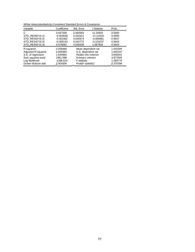
insignificant. Testing for non-captured ARCH effects by an LM test for four lags does not indicate

the presence of any such effects (Appendix 4), not rejecting the null of all the coefficients of the

squared residuals being jointly zero (F-stat=1.069770(0.3703)). However, we may observe the

marginal significance of the fourth lag.

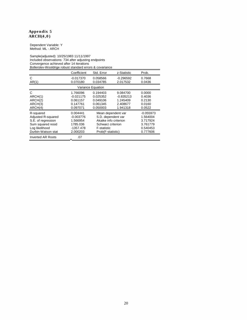
In light of this, we estimate an ARCH(4,0) and compare it with the previous one. As resulting from

Appendix 5, the a4 coefficient is significant. A Wald test for a4=0 rejects the null hypothesis.

Wald Test:

Equation: AR1

Null Hypothesis: C(7)=0

F-statistic 3.768717 Probability 0.052606

Chi-square 3.768717 Probability 0.052220

1 I apologise for the rather huge number of Appendices but there was a trade-off between covering my statements with statistical output and providing a reasonably thin paper. I preffered to choose the first alternative 2 All the GARCH estimation were carried in Eviews3.1 using the BHHH algorithm 3 Alternatively, we could use the t distribution

0

20

40

60

80

100

-3 -2 -1 0 1 2 3

Series : Standardized Res idualsSample 10/25/1983 11/11/1997Observations 734

Mean -0.012819Median -0.017086Maximum 3.346834Minimum -3.511669Std. Dev . 1.000602Skewness -0.007299Kurtos is 3.690840

Jarque-Bera 14.60274Probability 0.000675

6

As any ARCH model might have a more parsimonious GARCH representation (Bollerslev 1986,

Boero 2000), the next step was to incorporate a GARCH term and test for its significance, as well

as observing how the significance of the ARCH terms modifies. We thus estimated models that

allow the conditional variance to be an ARMA process:

),0(~/)()(

1

2

11

ttt

ttt

ttt

hNwherehLBLAh

ycy

−

−

Ω+=

+Φ+=

εε

ε

(4)

where B(L) is a lag polynomial of order n.

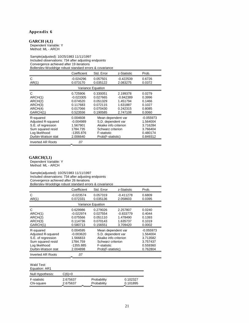
The first GARCH model we estimate has m=4 and n=1 (i.e. there is a GARCH(4,1))4 and we present

the estimation output in Appendix 6. Observing that judging by the t-statistics the ARCH terms

appear to be non-significant, we performed a Wald test for their joint significance (H0: all ai=0).

The hypothesis is rejected at the 10% level but not at the 5% level.

Wald Test:

Null Hypothesis: aI=0 for all i



We thus try to adopt a general-to-specific approach in reducing the number of lags in the ARCH

process. Testing for a4 =0 is not rejected. Wald Test:

Null Hypothesis: a4=0



We thus move to estimating GARCH(3,1) presenting the results in Appendix 6 together with a

Wald test for a3=0 which cannot be rejected even at 10% significance.

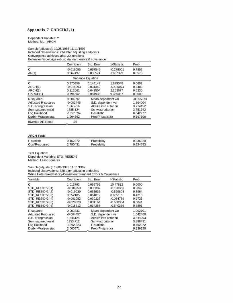
In light of this, we estimate a GARCH(2,1) (Appendix 7). The hypothesis a2=0 is now rejected at a

0.0238 level. Wald Test:

Null Hypothesis: a2=0



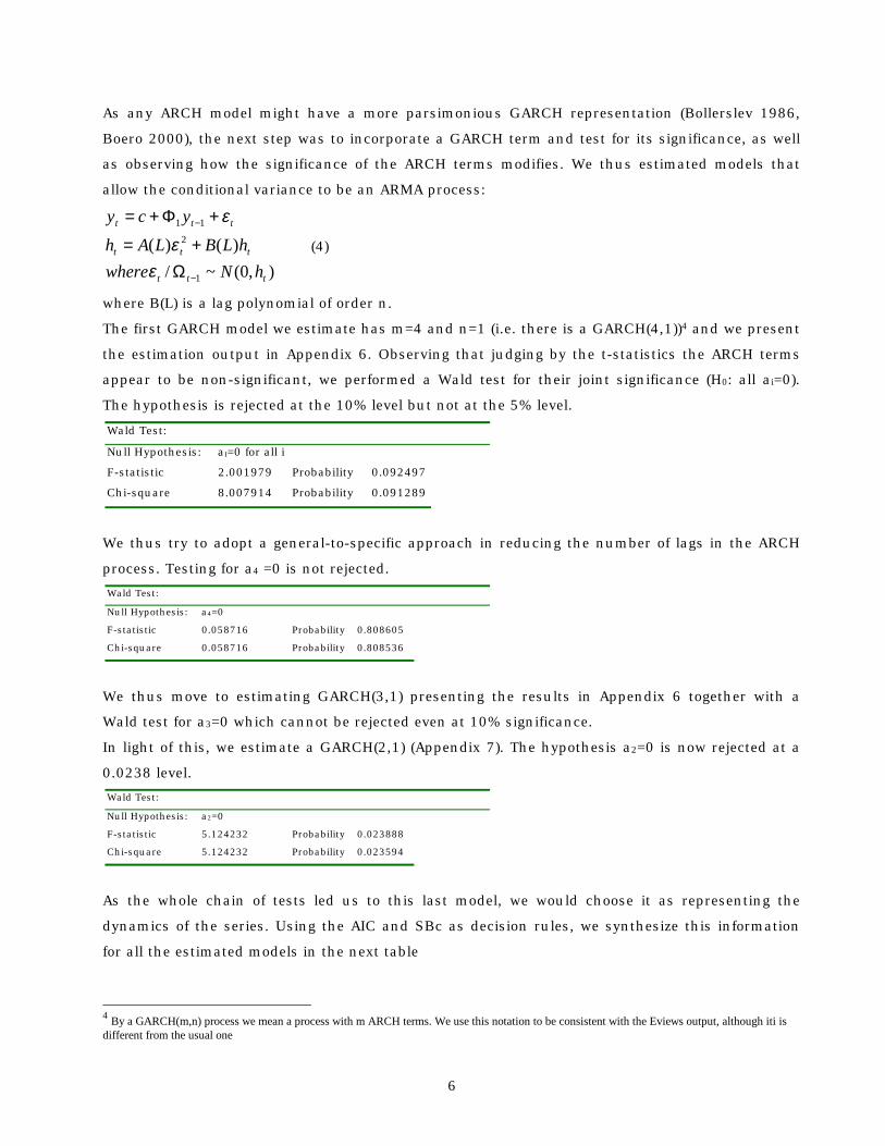
As the whole chain of tests led us to this last model, we would choose it as representing the

dynamics of the series. Using the AIC and SBc as decision rules, we synthesize this information

for all the estimated models in the next table

4 By a GARCH(m,n) process we mean a process with m ARCH terms. We use this notation to be consistent with the Eviews output, although iti is different from the usual one

7

Tests for AR(1) - GARCH(m,n) models, QML estimation, Bolerslev-Wooldridge Corrected Std Errors

ARCH(3,0) ARCH(4,0) GARCH(4,1) GARCH(3,1) GARCH(2,1)

JB* 14.60274 12.10750 12.28501 12.16835 14.26392

ARCH(4)** 0.370396 0.987807 0.992430 0.997868 0.702314

AIC 3.724227 3.717924 3.716284 3.713582 3.714152

SBC 3.761817 3.761779 3.766404 3.757437 3.751742

*test values, ** significance levels

Not surprisingly, the conclusion from the AIC is different from the one based on SBC as the last

one penalizes for the extra lags. However, since based on the Wald test we could reject the 3rd-

order term in the ARCH we choose the GARCH(2,1) model to describe the dynamics as it is more

parsimonious. We will thus use this model in the subsequent analysis.

Further analysis

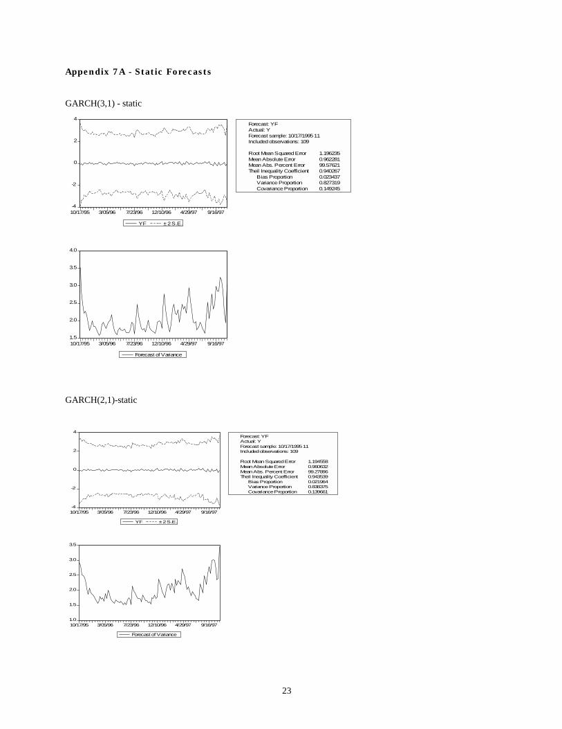
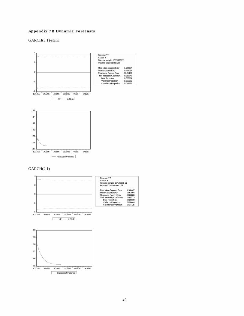
In terms of forecasting, we again tried to compare the GARCH(2,1) and GARCH(3,1) models,

presenting the results in Appendices 7A and 7B. The forecasts are made over the period

11:10:1995-11:11:1997 with the corresponding models5. Again, the GARCH(2,1) model performs

better in terms of forecasting (static), judging by the RMSE of 1.194558 compared to 1.196235 for

GARCH(2,1). For the dynamic method the values are 1.188447 as opposed to 1.189657

respectively.

We observe that the sum a1+a2+b1=0.892 implying that the volatility shocks are persistent in the

returns of the exchange rate, which comes as no surprise for the chosen high-frequency series.

The IGARCH hypothesis has been tested and reported below:

Wald Test: Equation: AR1 Null Hypothesis:

C(4)+C(5)+C(6)=1

F-statistic 3.507739 Probability 0.061483 Chi-square 3.507739 Probability 0.061083

This fact makes also the forecast of the conditional variance converge to the steady state rather

slowly (appendices 7ab). However, the process does not explode (sum of coefficients=1 rejected at

10%), which is consistent with the results rejection of a unit root. We also observe that a1<0, but

the conditional variance may still be well specified since it is of a rather small magnitude and is

not significant statistically (the probability of the t-statistic is 0.6483).

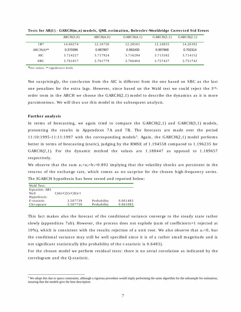
For the chosen model we perform residual tests: there is no serial correlation as indicated by the

correlogram and the Q-statistic.

5 We adopt this due to space constraints, although a rigorous procedure would imply performing the same algorithm for the subsample for estimation, insuring that the models give the best description

8

Q-statistic probabilities adjusted for 1 ARMA term(s)


.|. | .|. | 1 0.009 0.009 0.0562 .|. | .|. | 2 0.034 0.034 0.9021 0.342 .|. | .|. | 3 0.035 0.034 1.7915 0.408 .|. | .|. | 4 -0.027 -0.028 2.3126 0.510 .|. | .|. | 5 0.020 0.018 2.5980 0.627 .|. | .|. | 6 0.018 0.019 2.8422 0.724 .|. | .|. | 7 -0.010 -0.009 2.9117 0.820 .|. | .|. | 8 0.028 0.025 3.5034 0.835 .|. | .|. | 9 0.006 0.006 3.5320 0.897 .|. | .|. | 10 0.025 0.024 3.9831 0.913 .|. | .|. | 11 -0.034 -0.038 4.8227 0.903 .|. | .|. | 12 0.019 0.019 5.1010 0.926 .|. | .|. | 13 -0.009 -0.009 5.1619 0.952 .|. | .|. | 14 0.025 0.026 5.6147 0.959 .|. | .|. | 15 0.059 0.056 8.2415 0.876 .|. | .|. | 16 -0.031 -0.033 8.9773 0.879 .|. | .|. | 17 0.018 0.013 9.2090 0.905 .|. | .|. | 18 -0.032 -0.035 9.9716 0.905 .|. | .|. | 19 0.002 0.008 9.9733 0.933 .|. | .|. | 20 -0.004 -0.009 9.9836 0.953 .|. | .|. | 21 0.004 0.009 9.9959 0.968 .|. | .|. | 22 0.004 0.001 10.010 0.979 .|. | .|. | 23 0.041 0.040 11.292 0.970 .|. | .|. | 24 -0.041 -0.043 12.568 0.961

The ARCH LM test indicates that there are no ARCH effects not captured by the model. (please see

Appendix 7), the probability attached to the TR2 being 0.8346 and thus not rejecting the 'no-

further-ARCH' hypothesis.

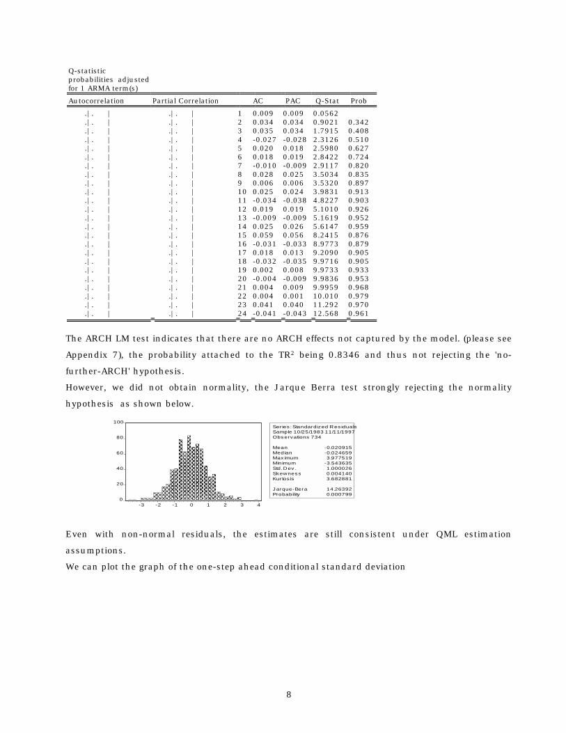
However, we did not obtain normality, the Jarque Berra test strongly rejecting the normality

hypothesis as shown below.

Even with non-normal residuals, the estimates are still consistent under QML estimation

assumptions.

We can plot the graph of the one-step ahead conditional standard deviation

0

20

40

60

80

100

-3 -2 -1 0 1 2 3 4

Series : Standardized Res idualsSample 10/25/1983 11/11/1997Obs ervations 734

Mean -0.020915Median -0.024659Max imum 3.977519Minimum -3.543635Std. Dev . 1.000026Skewness 0.004140Kurtos is 3.682881

J arque-Bera 14.26392Probability 0.000799

9

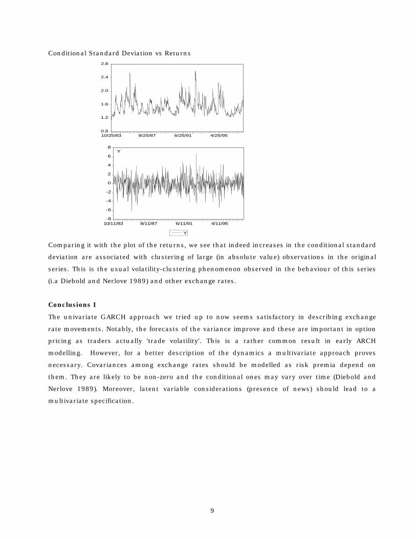
Conditional Standard Deviation vs Returns

Comparing it with the plot of the returns, we see that indeed increases in the conditional standard

deviation are associated with clustering of large (in absolute value) observations in the original

series. This is the usual volatility-clustering phenomenon observed in the behaviour of this series

(i.a Diebold and Nerlove 1989) and other exchange rates.

Conclusions I

The univariate GARCH approach we tried up to now seems satisfactory in describing exchange

rate movements. Notably, the forecasts of the variance improve and these are important in option

pricing as traders actually 'trade volatility'. This is a rather common result in early ARCH

modelling. However, for a better description of the dynamics a multivariate approach proves

necessary. Covariances among exchange rates should be modelled as risk premia depend on

them. They are likely to be non-zero and the conditional ones may vary over time (Diebold and

Nerlove 1989). Moreover, latent variable considerations (presence of news) should lead to a

multivariate specification.

0.8

1.2

1.6

2.0

2.4

2.8

10/25/83 8/25/87 6/25/91 4/25/95

-8

-6

-4

-2

0

2

4

6

8

10/11/83 8/11/87 6/11/91 4/11/95

Y

Y

10

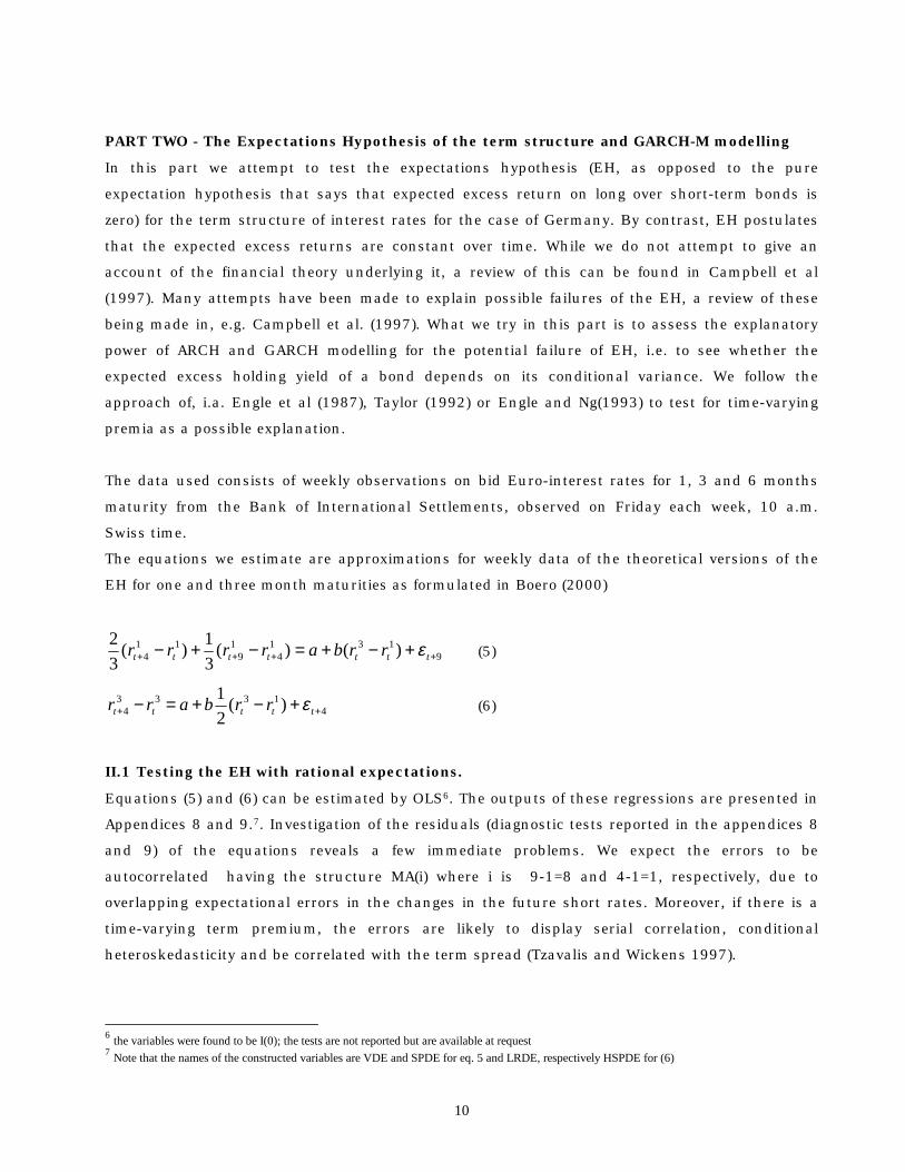
PART TWO - The Expectations Hypothesis of the term structure and GARCH-M modelling

In this part we attempt to test the expectations hypothesis (EH, as opposed to the pure

expectation hypothesis that says that expected excess return on long over short-term bonds is

zero) for the term structure of interest rates for the case of Germany. By contrast, EH postulates

that the expected excess returns are constant over time. While we do not attempt to give an

account of the financial theory underlying it, a review of this can be found in Campbell et al

(1997). Many attempts have been made to explain possible failures of the EH, a review of these

being made in, e.g. Campbell et al. (1997). What we try in this part is to assess the explanatory

power of ARCH and GARCH modelling for the potential failure of EH, i.e. to see whether the

expected excess holding yield of a bond depends on its conditional variance. We follow the

approach of, i.a. Engle et al (1987), Taylor (1992) or Engle and Ng(1993) to test for time-varying

premia as a possible explanation.

The data used consists of weekly observations on bid Euro-interest rates for 1, 3 and 6 months

maturity from the Bank of International Settlements, observed on Friday each week, 10 a.m.

Swiss time.

The equations we estimate are approximations for weekly data of the theoretical versions of the

EH for one and three month maturities as formulated in Boero (2000)

9131

41

911

4 )()(31)(

32

++++ +−+=−+− ttttttt rrbarrrr ε (5)

41333

4 )(21

++ +−+=− ttttt rrbarr ε (6)

II.1 Testing the EH with rational expectations.

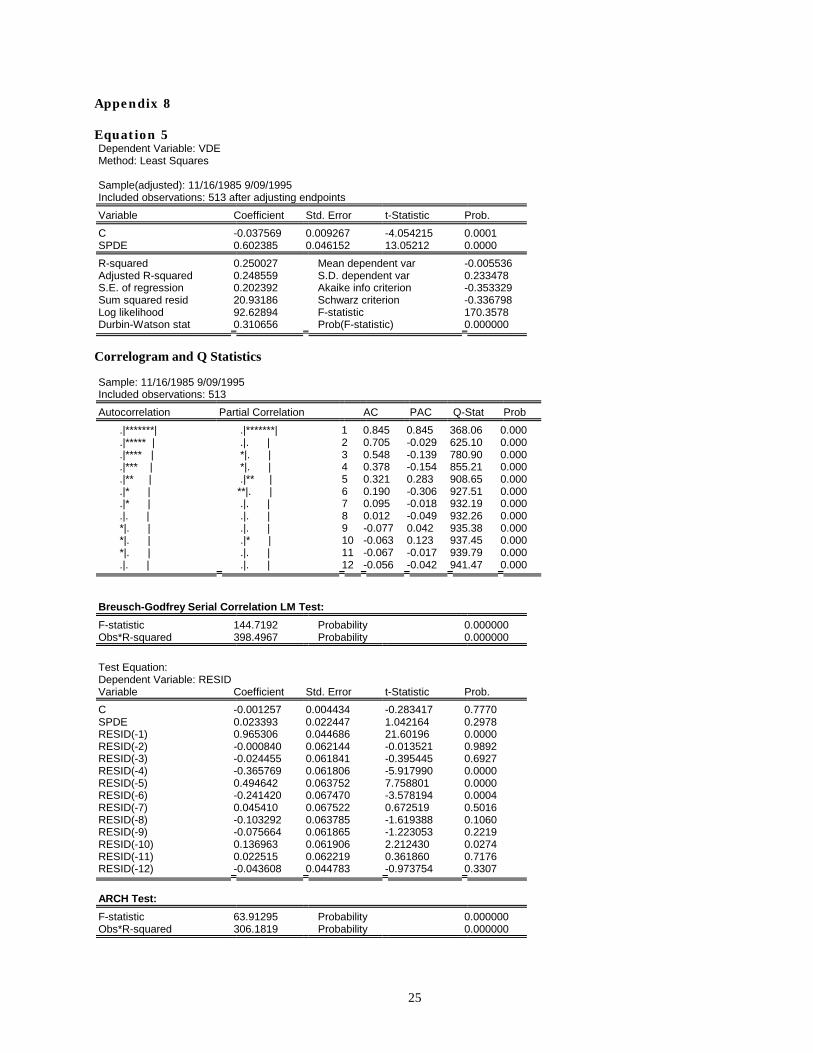
Equations (5) and (6) can be estimated by OLS6. The outputs of these regressions are presented in

Appendices 8 and 9.7. Investigation of the residuals (diagnostic tests reported in the appendices 8

and 9) of the equations reveals a few immediate problems. We expect the errors to be

autocorrelated having the structure MA(i) where i is 9-1=8 and 4-1=1, respectively, due to

overlapping expectational errors in the changes in the future short rates. Moreover, if there is a

time-varying term premium, the errors are likely to display serial correlation, conditional

heteroskedasticity and be correlated with the term spread (Tzavalis and Wickens 1997).

6 the variables were found to be I(0); the tests are not reported but are available at request 7 Note that the names of the constructed variables are VDE and SPDE for eq. 5 and LRDE, respectively HSPDE for (6)

11

Inspecting the diagnostic tests we find confirmation of the expected results: there are strong serial

correlation and ARCH effects as well as non-normality. Moreover, the correlograms of the

residuals resemble the structure of MA(8) and MA(3) data generating processes, as expected.

In order to perform the subsequent analysis we will thus have to use a correction of covariance

matrix, consistent with the presence of heteroskedasticity and serial correlation of unknown form,

as the Newey-West correction provided by EViews. Estimation outputs using the corrected

standard errors are presented in the final sections of Appendices 8 and 9. These are the

representations we will use further.

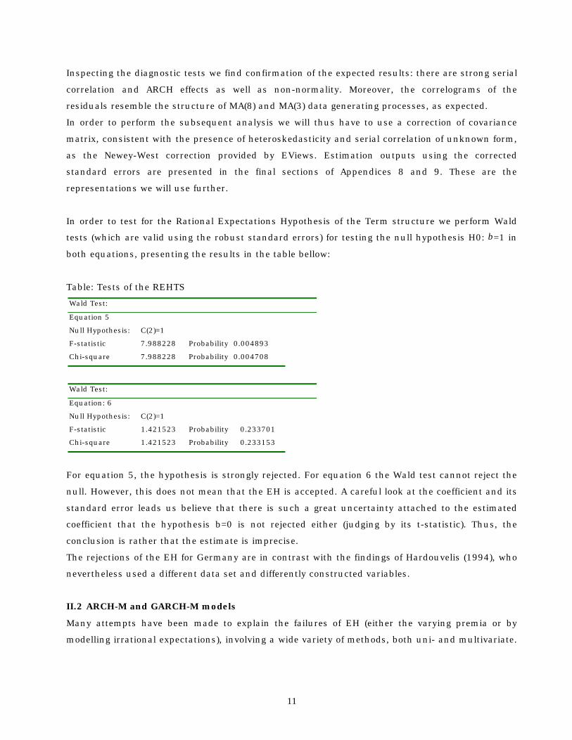
In order to test for the Rational Expectations Hypothesis of the Term structure we perform Wald

tests (which are valid using the robust standard errors) for testing the null hypothesis H0: b=1 in

both equations, presenting the results in the table bellow:

Table: Tests of the REHTS

Wald Test:

Equation 5




Wald Test:

Equation: 6




For equation 5, the hypothesis is strongly rejected. For equation 6 the Wald test cannot reject the

null. However, this does not mean that the EH is accepted. A careful look at the coefficient and its

standard error leads us believe that there is such a great uncertainty attached to the estimated

coefficient that the hypothesis b=0 is not rejected either (judging by its t-statistic). Thus, the

conclusion is rather that the estimate is imprecise.

The rejections of the EH for Germany are in contrast with the findings of Hardouvelis (1994), who

nevertheless used a different data set and differently constructed variables.

II.2 ARCH-M and GARCH-M models

Many attempts have been made to explain the failures of EH (either the varying premia or by

modelling irrational expectations), involving a wide variety of methods, both uni- and multivariate.

12

Here we just follow one of them, i.e. using ARCH in mean and GARCH in mean processes to take

into account a time varying term premium as pioneered by Engle et al(1987).

The argument for estimating such models runs as follows: variables with apparent explanatory

power for the dynamics of the spread (useful in forecasting excess returns) may be correlated with

the risk premia and thus would use their significance when a risk measure is included in the

regression.

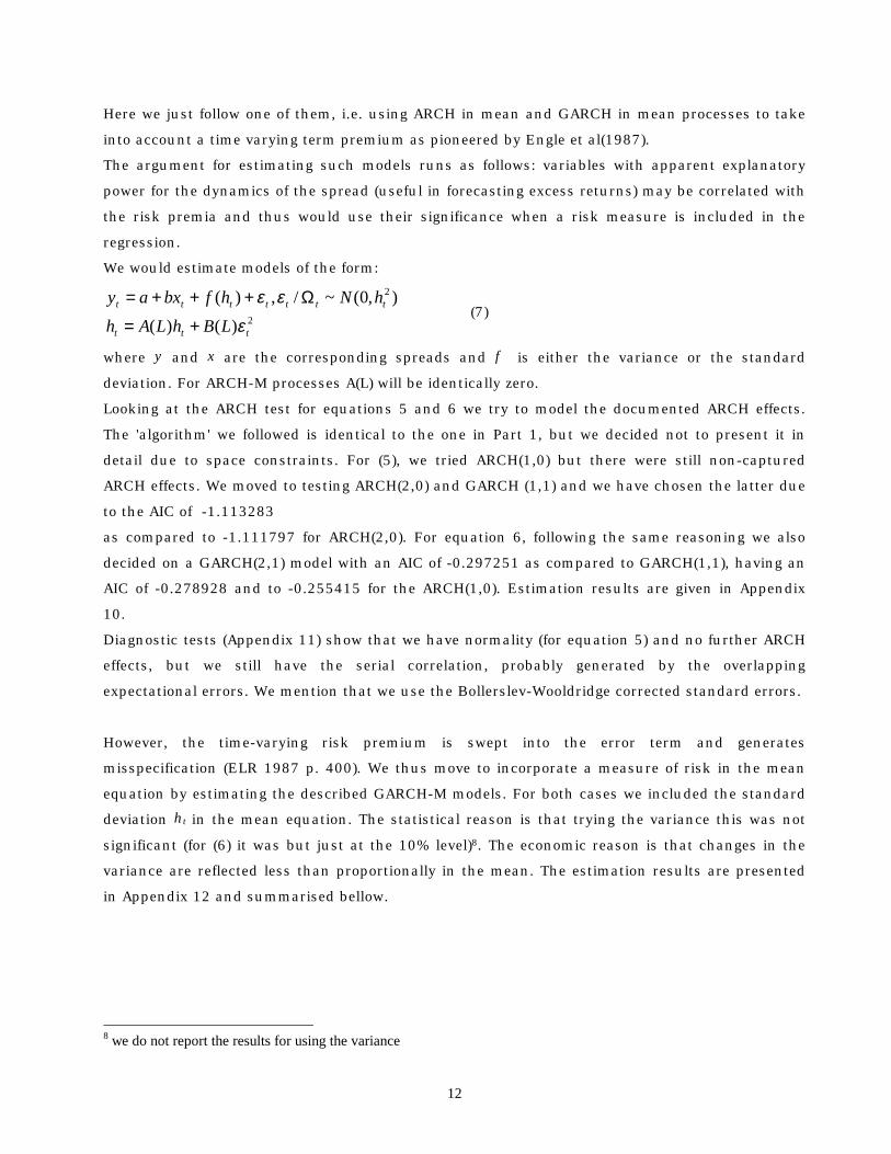
We would estimate models of the form:

2

2

)()(

),0(~/,)(

ttt

ttttttt

LBhLAhhNhfbxay

εεε

+=

Ω+++= (7)

where y and x are the corresponding spreads and f is either the variance or the standard

deviation. For ARCH-M processes A(L) will be identically zero.

Looking at the ARCH test for equations 5 and 6 we try to model the documented ARCH effects.

The 'algorithm' we followed is identical to the one in Part 1, but we decided not to present it in

detail due to space constraints. For (5), we tried ARCH(1,0) but there were still non-captured

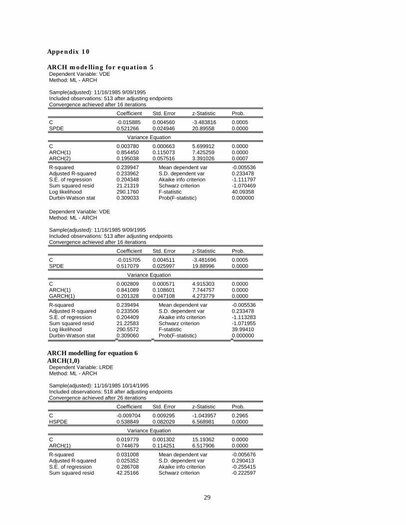
ARCH effects. We moved to testing ARCH(2,0) and GARCH (1,1) and we have chosen the latter due

to the AIC of -1.113283

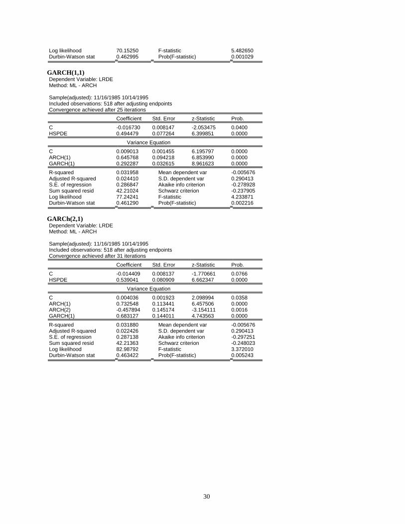
as compared to -1.111797 for ARCH(2,0). For equation 6, following the same reasoning we also

decided on a GARCH(2,1) model with an AIC of -0.297251 as compared to GARCH(1,1), having an

AIC of -0.278928 and to -0.255415 for the ARCH(1,0). Estimation results are given in Appendix

10.

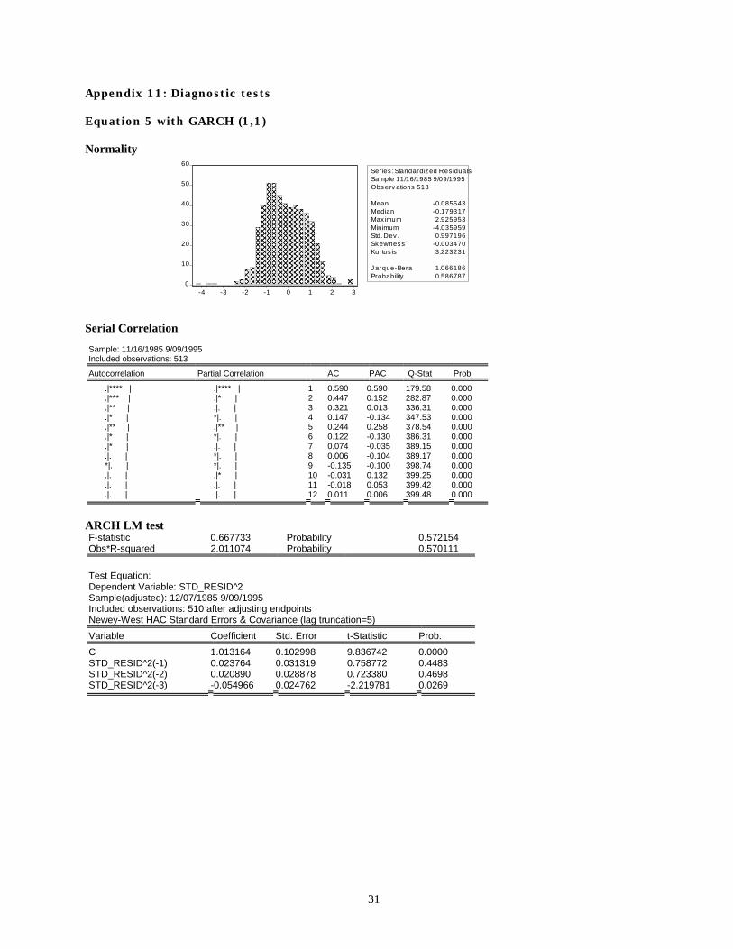
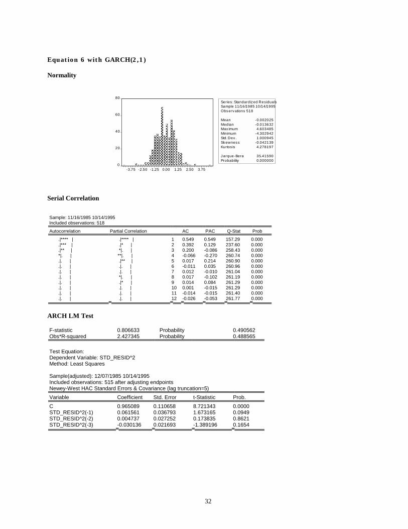
Diagnostic tests (Appendix 11) show that we have normality (for equation 5) and no further ARCH

effects, but we still have the serial correlation, probably generated by the overlapping

expectational errors. We mention that we use the Bollerslev-Wooldridge corrected standard errors.

However, the time-varying risk premium is swept into the error term and generates

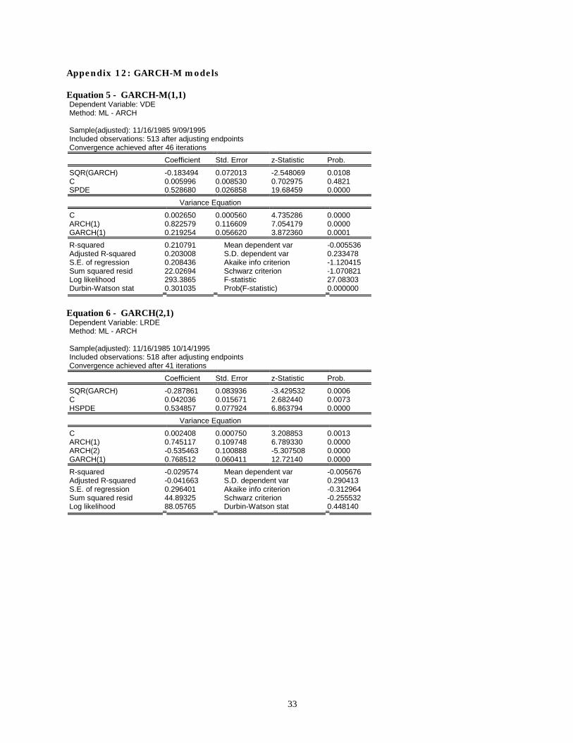
misspecification (ELR 1987 p. 400). We thus move to incorporate a measure of risk in the mean

equation by estimating the described GARCH-M models. For both cases we included the standard

deviation ht in the mean equation. The statistical reason is that trying the variance this was not

significant (for (6) it was but just at the 10% level)8. The economic reason is that changes in the

variance are reflected less than proportionally in the mean. The estimation results are presented

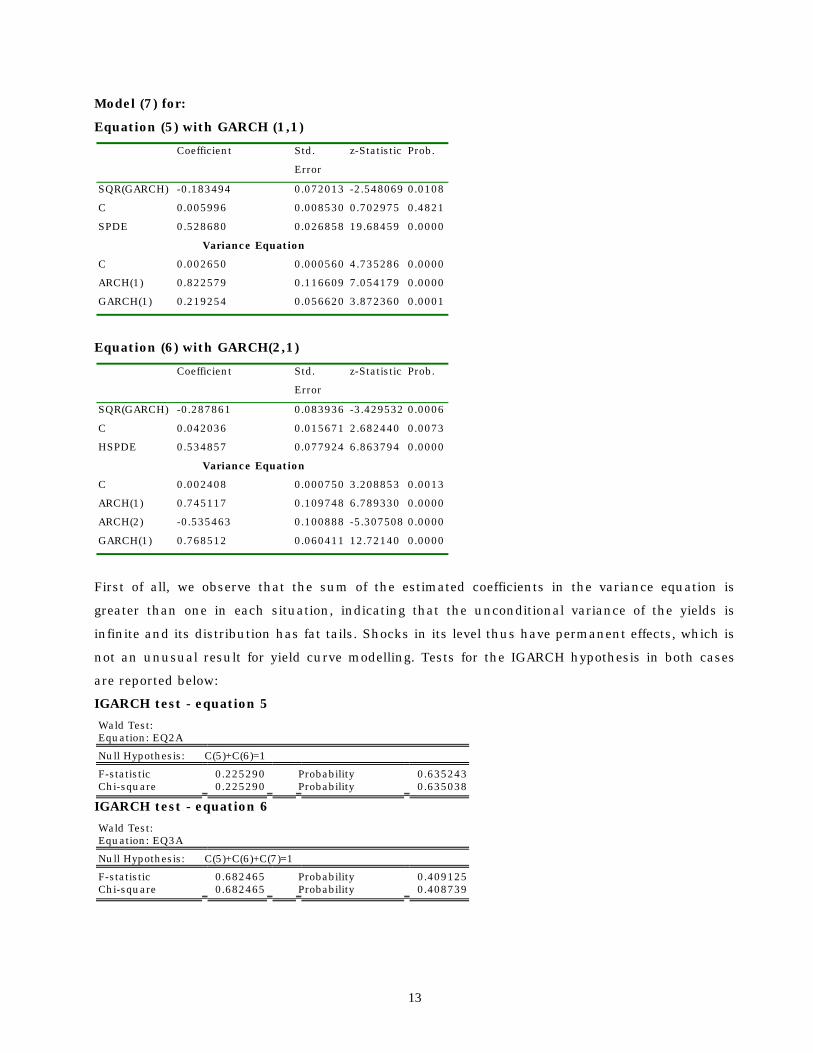
in Appendix 12 and summarised bellow.

8 we do not report the results for using the variance

13

Model (7) for: Equation (5) with GARCH (1,1) Coefficient Std.

Error

z-Statistic Prob.

SQR(GARCH) -0.183494 0.072013 -2.548069 0.0108

C 0.005996 0.008530 0.702975 0.4821

SPDE 0.528680 0.026858 19.68459 0.0000

Variance Equation C 0.002650 0.000560 4.735286 0.0000

ARCH(1) 0.822579 0.116609 7.054179 0.0000

GARCH(1) 0.219254 0.056620 3.872360 0.0001

Equation (6) with GARCH(2,1) Coefficient Std.

Error

z-Statistic Prob.

SQR(GARCH) -0.287861 0.083936 -3.429532 0.0006

C 0.042036 0.015671 2.682440 0.0073

HSPDE 0.534857 0.077924 6.863794 0.0000

Variance Equation C 0.002408 0.000750 3.208853 0.0013

ARCH(1) 0.745117 0.109748 6.789330 0.0000

ARCH(2) -0.535463 0.100888 -5.307508 0.0000

GARCH(1) 0.768512 0.060411 12.72140 0.0000

First of all, we observe that the sum of the estimated coefficients in the variance equation is

greater than one in each situation, indicating that the unconditional variance of the yields is

infinite and its distribution has fat tails. Shocks in its level thus have permanent effects, which is

not an unusual result for yield curve modelling. Tests for the IGARCH hypothesis in both cases

are reported below:

IGARCH test - equation 5 Wald Test: Equation: EQ2A

Null Hypothesis: C(5)+C(6)=1


IGARCH test - equation 6 Wald Test: Equation: EQ3A

Null Hypothesis: C(5)+C(6)+C(7)=1


14

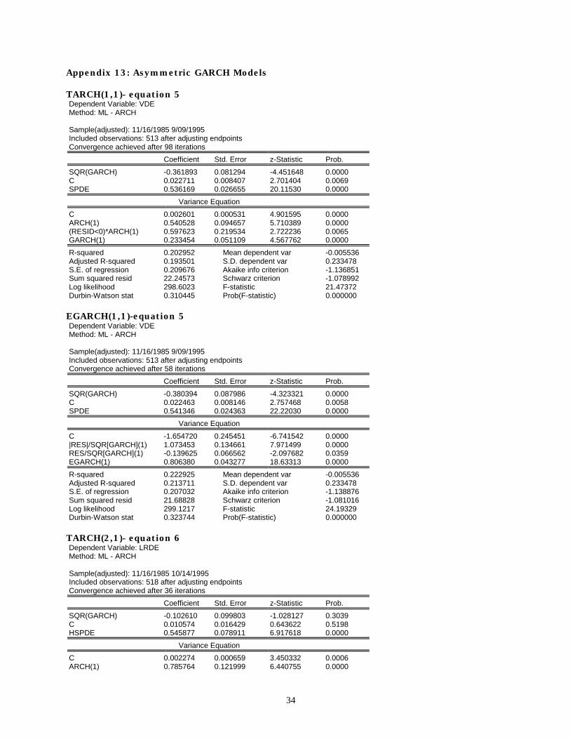
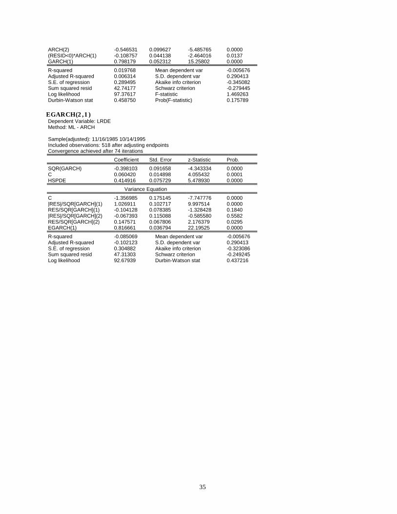
For completion, we also estimated TARCH and EGARCH models for the same specification in

order to take into account any asymmetric effects that are present9. While in all cases the

asymmetric terms are statistically significant, they do not change the main conclusions

(estimation outputs are presented in Appendix 13). Moreover, there is even a loss of statistical

significance in (6) of the standard deviation in the mean equation if we are to choose the TARCH

model as indicated by the AIC and SBC (Appendix 13).

Conclusions II

In contrast with the findings of ELR(1987), in our case introduction of a measure of risk does not

do a good job in explaining the time varying term premium. The coefficient on the spread in (5)

falls with 0.7 but its t-statistic actually rises. In equation (6) things are worse, the fall being of

0.05. However, the most important is the high statistical significance of the spread as opposed to

the uncertainty in the OLS case. These results are hardly consistent with the 'dramatic' fall in

ELR paper. However, the risk premium is statistically significant in explaining the time-varying

term premium. Nevertheless, the unsuccess in explaining the EH failure does not exclude the

possibility that another specification of the risk premium can do a better job (e.g. by taking into

account only systematic risk by using a time-varying beta CAPM for the term structure as

suggested by Taylor(1992)).

The failure of these simple models to explain why EH does not hold comes as no surprise. Even in

this univariate case, any omitted variable has been swept into the disturbance and thus all the

statistics are biased. In trying to explain failures of the EH it has been shown that multivariate

models can do a better job as in Campbell and Shiller (1987) or Taylor (1992). Moreover, as the

interest rates are also a policy variable, the relation between policy and the term spread needs to

be modelled (Boero and Torricelli, 1998). Thus, a system estimation in which a policy rule is

specified may prove necessary.

9 Presence of such effects can be more plausible in analysing interest rates on corporate bonds. However, we present the results for completion

15

Appendix 2: different models for the mean equation AR(1) Dependent Variable: Y Method: Least Squares Sample(adjusted): 10/25/1983 11/11/1997 Included observations: 734 after adjusting endpoints Convergence achieved after 3 iterations Variable Coefficient Std. Error t-Statistic Prob. C -0.056041 0.061995 -0.903958 0.3663 AR(1) 0.070505 0.036873 1.912117 0.0563 R-squared 0.004970 Mean dependent var -0.055973 Adjusted R-squared 0.003611 S.D. dependent var 1.564004 S.E. of regression 1.561178 Akaike info criterion 3.731480 Sum squared resid 1784.087 Schwarz criterion 3.744010 Log likelihood -1367.453 F-statistic 3.656190 Durbin-Watson stat 2.001929 Prob(F-statistic) 0.056251 Inverted AR Roots .07

MA(1) Dependent Variable: Y Method: Least Squares Sample(adjusted): 10/18/1983 11/11/1997 Included observations: 735 after adjusting endpoints Convergence achieved after 4 iterations Backcast: 10/11/1983 Variable Coefficient Std. Error t-Statistic Prob. C -0.055922 0.061464 -0.909837 0.3632 MA(1) 0.068095 0.036854 1.847711 0.0650 R-squared 0.004791 Mean dependent var -0.055870 Adjusted R-squared 0.003433 S.D. dependent var 1.562941 S.E. of regression 1.560256 Akaike info criterion 3.730294 Sum squared resid 1784.414 Schwarz criterion 3.742811 Log likelihood -1368.883 F-statistic 3.528396 Durbin-Watson stat 1.997202 Prob(F-statistic) 0.060723 Inverted MA Roots -.07

ARMA(1,1) Dependent Variable: Y Method: Least Squares Sample(adjusted): 10/25/1983 11/11/1997 Included observations: 734 after adjusting endpoints Convergence achieved after 15 iterations Backcast: 10/18/1983 Variable Coefficient Std. Error t-Statistic Prob. C -0.012954 0.017225 -0.752040 0.4523 AR(1) 0.802950 0.177154 4.532506 0.0000 MA(1) -0.766333 0.191243 -4.007111 0.0001 R-squared 0.006529 Mean dependent var -0.055973 Adjusted R-squared 0.003811 S.D. dependent var 1.564004 S.E. of regression 1.561022 Akaike info criterion 3.732637 Sum squared resid 1781.292 Schwarz criterion 3.751432 Log likelihood -1366.878 F-statistic 2.401922 Durbin-Watson stat 1.939587 Prob(F-statistic) 0.091258 Inverted MA Roots .77

16

Appendix 3: tests for AR(1) Histogram of residuals Correlogram of squared residuals Sample: 10/25/1983 11/11/1997 Included observations: 734 Q-statistic probabilities adjusted for 1 ARMA

term(s)

Autocorrelation Partial Correlation AC PAC Q-Stat Prob .|. | .|. | 1 -0.015 -0.015 0.1748 .|* | .|* | 2 0.068 0.068 3.6277 0.057 .|* | .|* | 3 0.079 0.082 8.2545 0.016 .|. | .|. | 4 0.058 0.057 10.754 0.013 .|. | .|. | 5 0.051 0.043 12.676 0.013 .|. | .|. | 6 0.019 0.007 12.941 0.024 .|. | .|. | 7 -0.004 -0.019 12.951 0.044 .|. | .|. | 8 0.052 0.040 14.990 0.036 .|. | *|. | 9 -0.057 -0.062 17.435 0.026 .|. | .|. | 10 0.024 0.014 17.871 0.037 .|* | .|* | 11 0.078 0.081 22.415 0.013 .|. | .|. | 12 0.023 0.030 22.811 0.019

LM test for serial correlation Breusch-Godfrey Serial Correlation LM Test: F-statistic 0.451528 Probability 0.844079 Obs*R-squared 2.728839 Probability 0.842029 Test Equation: Dependent Variable: RESID Method: Least Squares Presample missing value lagged residuals set to zero. Variable Coefficient Std. Error t-Statistic Prob. C -0.001912 0.062184 -0.030751 0.9755 AR(1) 14.61580 20.71762 0.705477 0.4807 RESID(-1) -14.61586 20.71772 -0.705476 0.4807 RESID(-2) -1.014079 1.461163 -0.694022 0.4879 RESID(-3) -0.046562 0.109488 -0.425267 0.6708 RESID(-4) -0.039859 0.037929 -1.050883 0.2937 RESID(-5) 0.028373 0.037250 0.761702 0.4465 RESID(-6) 0.007647 0.037264 0.205224 0.8375 R-squared 0.003718 Mean dependent var -2.21E-17 Adjusted R-squared -0.005888 S.D. dependent var 1.560113 S.E. of regression 1.564699 Akaike info criterion 3.744104 Sum squared resid 1777.454 Schwarz criterion 3.794224

0

20

40

60

80

100

120

-6 -4 -2 0 2 4 6

Series: Res idualsSample 10/25/1983 11/11/1997Obs erv ations 734

Mean -2.21E-17Median -0.007160Max imum 6.711607Minimum -6.148869Std. Dev . 1.560113Skewness -0.000997Kurtosis 4.002072


17

Log likelihood -1366.086 F-statistic 0.387024 Durbin-Watson stat 2.001730 Prob(F-statistic) 0.910188

ARCH Test: F-statistic 2.707074 Probability 0.029360 Obs*R-squared 10.74253 Probability 0.029615 Test Equation: Dependent Variable: RESID^2 Method: Least Squares Sample(adjusted): 11/22/1983 11/11/1997 Included observations: 730 after adjusting endpoints Variable Coefficient Std. Error t-Statistic Prob. C 1.999293 0.232183 8.610857 0.0000 RESID^2(-1) -0.024856 0.037083 -0.670287 0.5029 RESID^2(-2) 0.065177 0.036969 1.763008 0.0783 RESID^2(-3) 0.082937 0.037078 2.236820 0.0256 RESID^2(-4) 0.057166 0.037198 1.536823 0.1248 R-squared 0.014716 Mean dependent var 2.437385 Adjusted R-squared 0.009280 S.D. dependent var 4.223914 S.E. of regression 4.204270 Akaike info criterion 5.716904 Sum squared resid 12815.02 Schwarz criterion 5.748364 Log likelihood -2081.670 F-statistic 2.707074 Durbin-Watson stat 2.004755 Prob(F-statistic) 0.029360

18

Appendix 4 ARCH and GARCH models - estimation results ARCH (3,0) Dependent Variable: Y Method: ML - ARCH Sample(adjusted): 10/25/1983 11/11/1997 Included observations: 734 after adjusting endpoints Convergence achieved after 14 iterations Coefficient Std. Error z-Statistic Prob. C -0.030130 0.060166 -0.500775 0.6165 AR(1) 0.059383 0.036443 1.629498 0.1032 Variance Equation C 2.027690 0.153828 13.18152 0.0000 ARCH(1) -0.018993 0.025629 -0.741078 0.4586 ARCH(2) 0.057829 0.032991 1.752870 0.0796 ARCH(3) 0.131412 0.038958 3.373148 0.0007 R-squared 0.004603 Mean dependent var -0.055973 Adjusted R-squared -0.002233 S.D. dependent var 1.564004 S.E. of regression 1.565750 Akaike info criterion 3.724227 Sum squared resid 1784.745 Schwarz criterion 3.761817 Log likelihood -1360.791 F-statistic 0.673348 Durbin-Watson stat 1.978786 Prob(F-statistic) 0.643770 Inverted AR Roots .06

ARCH(3,0,) with corrected standard errors Dependent Variable: Y Method: ML - ARCH Sample(adjusted): 10/25/1983 11/11/1997 Included observations: 734 after adjusting endpoints Convergence achieved after 14 iterations Bollerslev-Wooldrige robust standard errors & covariance Coefficient Std. Error z-Statistic Prob. C -0.030130 0.059346 -0.507697 0.6117 AR(1) 0.059383 0.034433 1.724626 0.0846 Variance Equation C 2.027690 0.196954 10.29525 0.0000 ARCH(1) -0.018993 0.022351 -0.849773 0.3955 ARCH(2) 0.057829 0.046158 1.252838 0.2103 ARCH(3) 0.131412 0.060814 2.160892 0.0307 R-squared 0.004603 Mean dependent var -0.055973 Adjusted R-squared -0.002233 S.D. dependent var 1.564004 S.E. of regression 1.565750 Akaike info criterion 3.724227 Sum squared resid 1784.745 Schwarz criterion 3.761817 Log likelihood -1360.791 F-statistic 0.673348 Durbin-Watson stat 1.978786 Prob(F-statistic) 0.643770 Inverted AR Roots .06

ARCH Test: F-statistic 1.069770 Probability 0.370396 Obs*R-squared 4.283311 Probability 0.369020 Test Equation: Dependent Variable: STD_RESID^2 Method: Least Squares Sample(adjusted): 11/22/1983 11/11/1997 Included observations: 730 after adjusting endpoints

19

White Heteroskedasticity-Consistent Standard Errors & Covariance Variable Coefficient Std. Error t-Statistic Prob. C 0.937338 0.082663 11.33933 0.0000 STD_RESID^2(-1) -0.003648 0.031911 -0.114316 0.9090 STD_RESID^2(-2) -0.002302 0.040474 -0.056881 0.9547 STD_RESID^2(-3) -0.005143 0.042772 -0.120237 0.9043 STD_RESID^2(-4) 0.076692 0.045436 1.687926 0.0919 R-squared 0.005868 Mean dependent var 1.002594 Adjusted R-squared 0.000383 S.D. dependent var 1.645197 S.E. of regression 1.644883 Akaike info criterion 3.840041 Sum squared resid 1961.588 Schwarz criterion 3.871500 Log likelihood -1396.615 F-statistic 1.069770 Durbin-Watson stat 2.004306 Prob(F-statistic) 0.370396

20

Appendix 5 ARCH(4,0) Dependent Variable: Y Method: ML - ARCH Sample(adjusted): 10/25/1983 11/11/1997 Included observations: 734 after adjusting endpoints Convergence achieved after 14 iterations Bollerslev-Wooldrige robust standard errors & covariance Coefficient Std. Error z-Statistic Prob. C -0.017370 0.058566 -0.296592 0.7668 AR(1) 0.070180 0.034785 2.017532 0.0436 Variance Equation C 1.766096 0.194403 9.084700 0.0000 ARCH(1) -0.021175 0.025352 -0.835213 0.4036 ARCH(2) 0.061157 0.049106 1.245409 0.2130 ARCH(3) 0.147761 0.061345 2.408677 0.0160 ARCH(4) 0.097071 0.050003 1.941318 0.0522 R-squared 0.004441 Mean dependent var -0.055973 Adjusted R-squared -0.003776 S.D. dependent var 1.564004 S.E. of regression 1.566954 Akaike info criterion 3.717924 Sum squared resid 1785.036 Schwarz criterion 3.761779 Log likelihood -1357.478 F-statistic 0.540453 Durbin-Watson stat 2.000203 Prob(F-statistic) 0.777606 Inverted AR Roots .07

21

Appendix 6 GARCH (4,1) Dependent Variable: Y Method: ML - ARCH Sample(adjusted): 10/25/1983 11/11/1997 Included observations: 734 after adjusting endpoints Convergence achieved after 19 iterations Bollerslev-Wooldrige robust standard errors & covariance Coefficient Std. Error z-Statistic Prob. C -0.024296 0.057501 -0.422539 0.6726 AR(1) 0.073170 0.035122 2.083275 0.0372 Variance Equation C 0.725906 0.330051 2.199378 0.0279 ARCH(1) -0.023305 0.027665 -0.842389 0.3996 ARCH(2) 0.074520 0.051329 1.451794 0.1466 ARCH(3) 0.117683 0.072115 1.631887 0.1027 ARCH(4) 0.017066 0.070430 0.242315 0.8085 GARCH(1) 0.523556 0.190585 2.747108 0.0060 R-squared 0.004608 Mean dependent var -0.055973 Adjusted R-squared -0.004989 S.D. dependent var 1.564004 S.E. of regression 1.567901 Akaike info criterion 3.716284 Sum squared resid 1784.735 Schwarz criterion 3.766404 Log likelihood -1355.876 F-statistic 0.480174 Durbin-Watson stat 2.006640 Prob(F-statistic) 0.849312 Inverted AR Roots .07

GARCH(3,1) Dependent Variable: Y Method: ML - ARCH Sample(adjusted): 10/25/1983 11/11/1997 Included observations: 734 after adjusting endpoints Convergence achieved after 26 iterations Bollerslev-Wooldrige robust standard errors & covariance Coefficient Std. Error z-Statistic Prob. C -0.023574 0.057319 -0.411278 0.6809 AR(1) 0.072331 0.035136 2.058603 0.0395 Variance Equation C 0.629986 0.279026 2.257807 0.0240 ARCH(1) -0.022974 0.027554 -0.833779 0.4044 ARCH(2) 0.075566 0.051110 1.478490 0.1393 ARCH(3) 0.114736 0.070143 1.635737 0.1019 GARCH(1) 0.580713 0.156551 3.709420 0.0002 R-squared 0.004595 Mean dependent var -0.055973 Adjusted R-squared -0.003620 S.D. dependent var 1.564004 S.E. of regression 1.566833 Akaike info criterion 3.713582 Sum squared resid 1784.759 Schwarz criterion 3.757437 Log likelihood -1355.885 F-statistic 0.559360 Durbin-Watson stat 2.004898 Prob(F-statistic) 0.762804 Inverted AR Roots .07

Wald Test: Equation: AR1 Null Hypothesis: C(6)=0 F-statistic 2.675637 Probability 0.102327 Chi-square 2.675637 Probability 0.101895

22

Appendix 7 GARCH(2,1) Dependent Variable: Y Method: ML - ARCH Sample(adjusted): 10/25/1983 11/11/1997 Included observations: 734 after adjusting endpoints Convergence achieved after 20 iterations Bollerslev-Wooldrige robust standard errors & covariance Coefficient Std. Error z-Statistic Prob. C -0.016055 0.057546 -0.279001 0.7802 AR(1) 0.067497 0.035574 1.897329 0.0578 Variance Equation C 0.270859 0.144147 1.879048 0.0602 ARCH(1) -0.014293 0.031340 -0.456074 0.6483 ARCH(2) 0.112061 0.049504 2.263677 0.0236 GARCH(1) 0.794662 0.084935 9.356087 0.0000 R-squared 0.004392 Mean dependent var -0.055973 Adjusted R-squared -0.002446 S.D. dependent var 1.564004 S.E. of regression 1.565916 Akaike info criterion 3.714152 Sum squared resid 1785.124 Schwarz criterion 3.751742 Log likelihood -1357.094 F-statistic 0.642277 Durbin-Watson stat 1.994662 Prob(F-statistic) 0.667506 Inverted AR Roots .07

ARCH Test: F-statistic 0.462372 Probability 0.836320 Obs*R-squared 2.790431 Probability 0.834653 Test Equation: Dependent Variable: STD_RESID^2 Method: Least Squares Sample(adjusted): 12/06/1983 11/11/1997 Included observations: 728 after adjusting endpoints White Heteroskedasticity-Consistent Standard Errors & Covariance Variable Coefficient Std. Error t-Statistic Prob. C 1.013793 0.096752 10.47832 0.0000 STD_RESID^2(-1) -0.004259 0.035387 -0.120366 0.9042 STD_RESID^2(-2) -0.019039 0.035936 -0.529808 0.5964 STD_RESID^2(-3) 0.052185 0.064812 0.805185 0.4210 STD_RESID^2(-4) -0.001052 0.030228 -0.034789 0.9723 STD_RESID^2(-5) -0.020828 0.031164 -0.668334 0.5041 STD_RESID^2(-6) -0.018512 0.034258 -0.540359 0.5891 R-squared 0.003833 Mean dependent var 1.002101 Adjusted R-squared -0.004457 S.D. dependent var 1.642468 S.E. of regression 1.646124 Akaike info criterion 3.844293 Sum squared resid 1953.712 Schwarz criterion 3.888431 Log likelihood -1392.323 F-statistic 0.462372 Durbin-Watson stat 2.000571 Prob(F-statistic) 0.836320

23

Appendix 7A - Static Forecasts GARCH(3,1) - static GARCH(2,1)-static

-4

-2

0

2

4

10/17/95 3/05/96 7/23/96 12/10/96 4/29/97 9/16/97

YF ± 2 S.E.

Forecast: YFActual: YForecast sample: 10/17/1995 11Included observations: 109

Root Mean Squared Error 1.196235Mean Absolute Error 0.962281Mean Abs. Percent Error 99.57621Theil Inequality Coefficient 0.940267 Bias Proportion 0.023437 Variance Proportion 0.827319 Covariance Proportion 0.149245

1.5

2.0

2.5

3.0

3.5

4.0

10/17/95 3/05/96 7/23/96 12/10/96 4/29/97 9/16/97

Forecast of Variance

-4

-2

0

2

4

10/17/95 3/05/96 7/23/96 12/10/96 4/29/97 9/16/97

YF ± 2 S.E.



1.0

1.5

2.0

2.5

3.0

3.5

10/17/95 3/05/96 7/23/96 12/10/96 4/29/97 9/16/97


24

Appendix 7B Dynamic Forecasts GARCH(3,1)-static GARCH(2,1)

-4

-2

0

2

4

10/17/95 3/05/96 7/23/96 12/10/96 4/29/97 9/16/97

YF ± 2 S.E.



2.4

2.6

2.8

3.0

3.2

3.4

3.6

10/17/95 3/05/96 7/23/96 12/10/96 4/29/97 9/16/97


-4

-2

0

2

4

10/17/95 3/05/96 7/23/96 12/10/96 4/29/97 9/16/97

YF ± 2 S.E.



2.5

2.6

2.7

2.8

2.9

3.0

10/17/95 3/05/96 7/23/96 12/10/96 4/29/97 9/16/97


25

Appendix 8 Equation 5 Dependent Variable: VDE Method: Least Squares Sample(adjusted): 11/16/1985 9/09/1995 Included observations: 513 after adjusting endpoints Variable Coefficient Std. Error t-Statistic Prob. C -0.037569 0.009267 -4.054215 0.0001 SPDE 0.602385 0.046152 13.05212 0.0000 R-squared 0.250027 Mean dependent var -0.005536 Adjusted R-squared 0.248559 S.D. dependent var 0.233478 S.E. of regression 0.202392 Akaike info criterion -0.353329 Sum squared resid 20.93186 Schwarz criterion -0.336798 Log likelihood 92.62894 F-statistic 170.3578 Durbin-Watson stat 0.310656 Prob(F-statistic) 0.000000

Correlogram and Q Statistics Sample: 11/16/1985 9/09/1995 Included observations: 513 Autocorrelation Partial Correlation AC PAC Q-Stat Prob .|*******| .|*******| 1 0.845 0.845 368.06 0.000 .|***** | .|. | 2 0.705 -0.029 625.10 0.000 .|**** | *|. | 3 0.548 -0.139 780.90 0.000 .|*** | *|. | 4 0.378 -0.154 855.21 0.000 .|** | .|** | 5 0.321 0.283 908.65 0.000 .|* | **|. | 6 0.190 -0.306 927.51 0.000 .|* | .|. | 7 0.095 -0.018 932.19 0.000 .|. | .|. | 8 0.012 -0.049 932.26 0.000 *|. | .|. | 9 -0.077 0.042 935.38 0.000 *|. | .|* | 10 -0.063 0.123 937.45 0.000 *|. | .|. | 11 -0.067 -0.017 939.79 0.000 .|. | .|. | 12 -0.056 -0.042 941.47 0.000

Breusch-Godfrey Serial Correlation LM Test: F-statistic 144.7192 Probability 0.000000 Obs*R-squared 398.4967 Probability 0.000000 Test Equation: Dependent Variable: RESID Variable Coefficient Std. Error t-Statistic Prob. C -0.001257 0.004434 -0.283417 0.7770 SPDE 0.023393 0.022447 1.042164 0.2978 RESID(-1) 0.965306 0.044686 21.60196 0.0000 RESID(-2) -0.000840 0.062144 -0.013521 0.9892 RESID(-3) -0.024455 0.061841 -0.395445 0.6927 RESID(-4) -0.365769 0.061806 -5.917990 0.0000 RESID(-5) 0.494642 0.063752 7.758801 0.0000 RESID(-6) -0.241420 0.067470 -3.578194 0.0004 RESID(-7) 0.045410 0.067522 0.672519 0.5016 RESID(-8) -0.103292 0.063785 -1.619388 0.1060 RESID(-9) -0.075664 0.061865 -1.223053 0.2219 RESID(-10) 0.136963 0.061906 2.212430 0.0274 RESID(-11) 0.022515 0.062219 0.361860 0.7176 RESID(-12) -0.043608 0.044783 -0.973754 0.3307

ARCH Test: F-statistic 63.91295 Probability 0.000000 Obs*R-squared 306.1819 Probability 0.000000

26

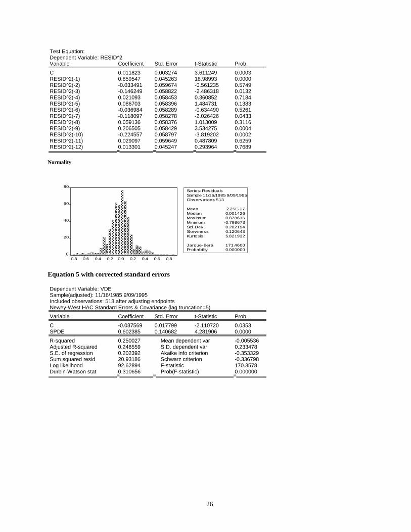
Test Equation: Dependent Variable: RESID^2 Variable Coefficient Std. Error t-Statistic Prob. C 0.011823 0.003274 3.611249 0.0003 RESID^2(-1) 0.859547 0.045263 18.98993 0.0000 RESID^2(-2) -0.033491 0.059674 -0.561235 0.5749 RESID^2(-3) -0.146249 0.058822 -2.486318 0.0132 RESID^2(-4) 0.021093 0.058453 0.360852 0.7184 RESID^2(-5) 0.086703 0.058396 1.484731 0.1383 RESID^2(-6) -0.036984 0.058289 -0.634490 0.5261 RESID^2(-7) -0.118097 0.058278 -2.026426 0.0433 RESID^2(-8) 0.059136 0.058376 1.013009 0.3116 RESID^2(-9) 0.206505 0.058429 3.534275 0.0004 RESID^2(-10) -0.224557 0.058797 -3.819202 0.0002 RESID^2(-11) 0.029097 0.059649 0.487809 0.6259 RESID^2(-12) 0.013301 0.045247 0.293964 0.7689

Normality Equation 5 with corrected standard errors Dependent Variable: VDE Sample(adjusted): 11/16/1985 9/09/1995 Included observations: 513 after adjusting endpoints Newey-West HAC Standard Errors & Covariance (lag truncation=5) Variable Coefficient Std. Error t-Statistic Prob. C -0.037569 0.017799 -2.110720 0.0353 SPDE 0.602385 0.140682 4.281906 0.0000 R-squared 0.250027 Mean dependent var -0.005536 Adjusted R-squared 0.248559 S.D. dependent var 0.233478 S.E. of regression 0.202392 Akaike info criterion -0.353329 Sum squared resid 20.93186 Schwarz criterion -0.336798 Log likelihood 92.62894 F-statistic 170.3578 Durbin-Watson stat 0.310656 Prob(F-statistic) 0.000000

0

20

40

60

80

-0.8 -0.6 -0.4 -0.2 0.0 0.2 0.4 0.6 0.8

Series: ResidualsSample 11/16/1985 9/09/1995Observations 513

Mean 2.25E-17Median 0.001426Maximum 0.878616Minimum -0.798673Std. Dev. 0.202194Skewness 0.120643Kurtosis 5.821932


27

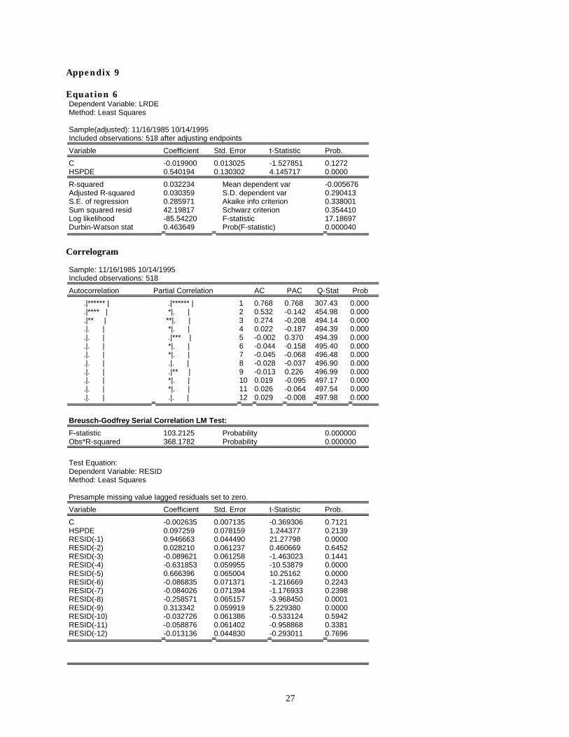
Appendix 9 Equation 6 Dependent Variable: LRDE Method: Least Squares Sample(adjusted): 11/16/1985 10/14/1995 Included observations: 518 after adjusting endpoints Variable Coefficient Std. Error t-Statistic Prob. C -0.019900 0.013025 -1.527851 0.1272 HSPDE 0.540194 0.130302 4.145717 0.0000 R-squared 0.032234 Mean dependent var -0.005676 Adjusted R-squared 0.030359 S.D. dependent var 0.290413 S.E. of regression 0.285971 Akaike info criterion 0.338001 Sum squared resid 42.19817 Schwarz criterion 0.354410 Log likelihood -85.54220 F-statistic 17.18697 Durbin-Watson stat 0.463649 Prob(F-statistic) 0.000040

Correlogram Sample: 11/16/1985 10/14/1995 Included observations: 518 Autocorrelation Partial Correlation AC PAC Q-Stat Prob .|****** | .|****** | 1 0.768 0.768 307.43 0.000 .|**** | *|. | 2 0.532 -0.142 454.98 0.000 .|** | **|. | 3 0.274 -0.208 494.14 0.000 .|. | *|. | 4 0.022 -0.187 494.39 0.000 .|. | .|*** | 5 -0.002 0.370 494.39 0.000 .|. | *|. | 6 -0.044 -0.158 495.40 0.000 .|. | *|. | 7 -0.045 -0.068 496.48 0.000 .|. | .|. | 8 -0.028 -0.037 496.90 0.000 .|. | .|** | 9 -0.013 0.226 496.99 0.000 .|. | *|. | 10 0.019 -0.095 497.17 0.000 .|. | *|. | 11 0.026 -0.064 497.54 0.000 .|. | .|. | 12 0.029 -0.008 497.98 0.000

Breusch-Godfrey Serial Correlation LM Test: F-statistic 103.2125 Probability 0.000000 Obs*R-squared 368.1782 Probability 0.000000 Test Equation: Dependent Variable: RESID Method: Least Squares Presample missing value lagged residuals set to zero. Variable Coefficient Std. Error t-Statistic Prob. C -0.002635 0.007135 -0.369306 0.7121 HSPDE 0.097259 0.078159 1.244377 0.2139 RESID(-1) 0.946663 0.044490 21.27798 0.0000 RESID(-2) 0.028210 0.061237 0.460669 0.6452 RESID(-3) -0.089621 0.061258 -1.463023 0.1441 RESID(-4) -0.631853 0.059955 -10.53879 0.0000 RESID(-5) 0.666396 0.065004 10.25162 0.0000 RESID(-6) -0.086835 0.071371 -1.216669 0.2243 RESID(-7) -0.084026 0.071394 -1.176933 0.2398 RESID(-8) -0.258571 0.065157 -3.968450 0.0001 RESID(-9) 0.313342 0.059919 5.229380 0.0000 RESID(-10) -0.032726 0.061386 -0.533124 0.5942 RESID(-11) -0.058876 0.061402 -0.958868 0.3381 RESID(-12) -0.013136 0.044830 -0.293011 0.7696

28

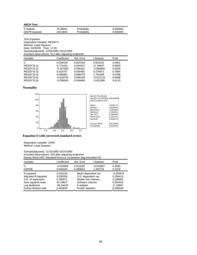
ARCH Test: F-statistic 76.38041 Probability 0.000000 Obs*R-squared 243.5844 Probability 0.000000 Test Equation: Dependent Variable: RESID^2 Method: Least Squares Date: 04/30/00 Time: 17:26 Sample(adjusted): 12/28/1985 10/14/1995 Included observations: 512 after adjusting endpoints Variable Coefficient Std. Error t-Statistic Prob. C 0.028428 0.007434 3.824152 0.0001 RESID^2(-1) 0.771410 0.044471 17.34647 0.0000 RESID^2(-2) -0.167628 0.056161 -2.984800 0.0030 RESID^2(-3) 0.015757 0.056481 0.278972 0.7804 RESID^2(-4) 0.099482 0.056479 1.761405 0.0788 RESID^2(-5) -0.028760 0.056159 -0.512119 0.6088 RESID^2(-6) -0.036549 0.044469 -0.821895 0.4115

Normality Equation 6 with corrected standard errors Dependent Variable: LRDE Method: Least Squares Sample(adjusted): 11/16/1985 10/14/1995 Included observations: 518 after adjusting endpoints Newey-West HAC Standard Errors & Covariance (lag truncation=5) Variable Coefficient Std. Error t-Statistic Prob. C -0.019900 0.021632 -0.919957 0.3580 HSPDE 0.540194 0.385654 1.400724 0.1619 R-squared 0.032234 Mean dependent var -0.005676 Adjusted R-squared 0.030359 S.D. dependent var 0.290413 S.E. of regression 0.285971 Akaike info criterion 0.338001 Sum squared resid 42.19817 Schwarz criterion 0.354410 Log likelihood -85.54220 F-statistic 17.18697 Durbin-Watson stat 0.463649 Prob(F-statistic) 0.000040

0

20

40

60

80

100

120

-1.0 -0.5 0.0 0.5 1.0

Series: Res idualsSample 11/16/1985 10/14/1995Observations 518

Mean 3.94E-17Median 0.003694Maximum 1.250993Minimum -1.293991Std. Dev. 0.285694Skewness 0.102411Kurtosis 6.858273


29

Appendix 10 ARCH modelling for equation 5 Dependent Variable: VDE Method: ML - ARCH Sample(adjusted): 11/16/1985 9/09/1995 Included observations: 513 after adjusting endpoints Convergence achieved after 16 iterations Coefficient Std. Error z-Statistic Prob. C -0.015885 0.004560 -3.483816 0.0005 SPDE 0.521266 0.024946 20.89558 0.0000 Variance Equation C 0.003780 0.000663 5.699912 0.0000 ARCH(1) 0.854450 0.115073 7.425259 0.0000 ARCH(2) 0.195038 0.057516 3.391026 0.0007 R-squared 0.239947 Mean dependent var -0.005536 Adjusted R-squared 0.233962 S.D. dependent var 0.233478 S.E. of regression 0.204348 Akaike info criterion -1.111797 Sum squared resid 21.21319 Schwarz criterion -1.070469 Log likelihood 290.1760 F-statistic 40.09358 Durbin-Watson stat 0.309033 Prob(F-statistic) 0.000000

Dependent Variable: VDE Method: ML - ARCH Sample(adjusted): 11/16/1985 9/09/1995 Included observations: 513 after adjusting endpoints Convergence achieved after 16 iterations Coefficient Std. Error z-Statistic Prob. C -0.015705 0.004511 -3.481696 0.0005 SPDE 0.517079 0.025997 19.88996 0.0000 Variance Equation C 0.002809 0.000571 4.915303 0.0000 ARCH(1) 0.841089 0.108601 7.744757 0.0000 GARCH(1) 0.201328 0.047108 4.273779 0.0000 R-squared 0.239494 Mean dependent var -0.005536 Adjusted R-squared 0.233506 S.D. dependent var 0.233478 S.E. of regression 0.204409 Akaike info criterion -1.113283 Sum squared resid 21.22583 Schwarz criterion -1.071955 Log likelihood 290.5572 F-statistic 39.99410 Durbin-Watson stat 0.309060 Prob(F-statistic) 0.000000

ARCH modelling for equation 6 ARCH(1,0) Dependent Variable: LRDE Method: ML - ARCH Sample(adjusted): 11/16/1985 10/14/1995 Included observations: 518 after adjusting endpoints Convergence achieved after 26 iterations Coefficient Std. Error z-Statistic Prob. C -0.009704 0.009295 -1.043957 0.2965 HSPDE 0.538849 0.082029 6.568981 0.0000 Variance Equation C 0.019779 0.001302 15.19362 0.0000 ARCH(1) 0.744679 0.114251 6.517906 0.0000 R-squared 0.031008 Mean dependent var -0.005676 Adjusted R-squared 0.025352 S.D. dependent var 0.290413 S.E. of regression 0.286708 Akaike info criterion -0.255415 Sum squared resid 42.25166 Schwarz criterion -0.222597

30

Log likelihood 70.15250 F-statistic 5.482650 Durbin-Watson stat 0.462995 Prob(F-statistic) 0.001029

GARCH(1,1) Dependent Variable: LRDE Method: ML - ARCH Sample(adjusted): 11/16/1985 10/14/1995 Included observations: 518 after adjusting endpoints Convergence achieved after 25 iterations Coefficient Std. Error z-Statistic Prob. C -0.016730 0.008147 -2.053475 0.0400 HSPDE 0.494479 0.077264 6.399851 0.0000 Variance Equation C 0.009013 0.001455 6.195797 0.0000 ARCH(1) 0.645768 0.094218 6.853990 0.0000 GARCH(1) 0.292287 0.032615 8.961623 0.0000 R-squared 0.031958 Mean dependent var -0.005676 Adjusted R-squared 0.024410 S.D. dependent var 0.290413 S.E. of regression 0.286847 Akaike info criterion -0.278928 Sum squared resid 42.21024 Schwarz criterion -0.237905 Log likelihood 77.24241 F-statistic 4.233871 Durbin-Watson stat 0.461290 Prob(F-statistic) 0.002216

GARCh(2,1) Dependent Variable: LRDE Method: ML - ARCH Sample(adjusted): 11/16/1985 10/14/1995 Included observations: 518 after adjusting endpoints Convergence achieved after 31 iterations Coefficient Std. Error z-Statistic Prob. C -0.014409 0.008137 -1.770661 0.0766 HSPDE 0.539041 0.080909 6.662347 0.0000 Variance Equation C 0.004036 0.001923 2.098994 0.0358 ARCH(1) 0.732548 0.113441 6.457506 0.0000 ARCH(2) -0.457894 0.145174 -3.154111 0.0016 GARCH(1) 0.683127 0.144011 4.743563 0.0000 R-squared 0.031880 Mean dependent var -0.005676 Adjusted R-squared 0.022426 S.D. dependent var 0.290413 S.E. of regression 0.287138 Akaike info criterion -0.297251 Sum squared resid 42.21363 Schwarz criterion -0.248023 Log likelihood 82.98792 F-statistic 3.372010 Durbin-Watson stat 0.463422 Prob(F-statistic) 0.005243

31

Appendix 11: Diagnostic tests Equation 5 with GARCH (1,1) Normality Serial Correlation Sample: 11/16/1985 9/09/1995 Included observations: 513


.|**** | .|**** | 1 0.590 0.590 179.58 0.000 .|*** | .|* | 2 0.447 0.152 282.87 0.000 .|** | .|. | 3 0.321 0.013 336.31 0.000 .|* | *|. | 4 0.147 -0.134 347.53 0.000 .|** | .|** | 5 0.244 0.258 378.54 0.000 .|* | *|. | 6 0.122 -0.130 386.31 0.000 .|* | .|. | 7 0.074 -0.035 389.15 0.000 .|. | *|. | 8 0.006 -0.104 389.17 0.000 *|. | *|. | 9 -0.135 -0.100 398.74 0.000 .|. | .|* | 10 -0.031 0.132 399.25 0.000 .|. | .|. | 11 -0.018 0.053 399.42 0.000 .|. | .|. | 12 0.011 0.006 399.48 0.000

ARCH LM test F-statistic 0.667733 Probability 0.572154 Obs*R-squared 2.011074 Probability 0.570111 Test Equation: Dependent Variable: STD_RESID^2 Sample(adjusted): 12/07/1985 9/09/1995 Included observations: 510 after adjusting endpoints Newey-West HAC Standard Errors & Covariance (lag truncation=5) Variable Coefficient Std. Error t-Statistic Prob. C 1.013164 0.102998 9.836742 0.0000 STD_RESID^2(-1) 0.023764 0.031319 0.758772 0.4483 STD_RESID^2(-2) 0.020890 0.028878 0.723380 0.4698 STD_RESID^2(-3) -0.054966 0.024762 -2.219781 0.0269

0

10

20

30

40

50

60

-4 -3 -2 -1 0 1 2 3

Series: Standardized ResidualsSample 11/16/1985 9/09/1995Observ ations 513

Mean -0.085543Median -0.179317Max imum 2.925953Minimum -4.035959Std. Dev . 0.997196Skewness -0.003470Kurtos is 3.223231


32

Equation 6 with GARCH(2,1) Normality Serial Correlation Sample: 11/16/1985 10/14/1995 Included observations: 518


.|**** | .|**** | 1 0.549 0.549 157.29 0.000 .|*** | .|* | 2 0.392 0.129 237.60 0.000 .|** | *|. | 3 0.200 -0.086 258.43 0.000 *|. | **|. | 4 -0.066 -0.270 260.74 0.000 .|. | .|** | 5 0.017 0.214 260.90 0.000 .|. | .|. | 6 -0.011 0.035 260.96 0.000 .|. | .|. | 7 0.012 -0.010 261.04 0.000 .|. | *|. | 8 0.017 -0.102 261.19 0.000 .|. | .|* | 9 0.014 0.084 261.29 0.000 .|. | .|. | 10 0.001 -0.015 261.29 0.000 .|. | .|. | 11 -0.014 -0.015 261.40 0.000 .|. | .|. | 12 -0.026 -0.053 261.77 0.000

ARCH LM Test F-statistic 0.806633 Probability 0.490562 Obs*R-squared 2.427345 Probability 0.488565 Test Equation: Dependent Variable: STD_RESID^2 Method: Least Squares Sample(adjusted): 12/07/1985 10/14/1995 Included observations: 515 after adjusting endpoints Newey-West HAC Standard Errors & Covariance (lag truncation=5) Variable Coefficient Std. Error t-Statistic Prob. C 0.965089 0.110658 8.721343 0.0000 STD_RESID^2(-1) 0.061561 0.036793 1.673165 0.0949 STD_RESID^2(-2) 0.004737 0.027252 0.173835 0.8621 STD_RESID^2(-3) -0.030136 0.021693 -1.389196 0.1654

0

20

40

60

80

-3.75 -2.50 -1.25 0.00 1.25 2.50 3.75

Series: Standardized ResidualsSample 11/16/1985 10/14/1995Observ ations 518

Mean -0.002025Median -0.013632Max imum 4.603485Minimum -4.302942Std. Dev . 1.000945Skewness -0.042139Kurtos is 4.278197


33

Appendix 12: GARCH-M models Equation 5 - GARCH-M(1,1) Dependent Variable: VDE Method: ML - ARCH Sample(adjusted): 11/16/1985 9/09/1995 Included observations: 513 after adjusting endpoints Convergence achieved after 46 iterations Coefficient Std. Error z-Statistic Prob. SQR(GARCH) -0.183494 0.072013 -2.548069 0.0108 C 0.005996 0.008530 0.702975 0.4821 SPDE 0.528680 0.026858 19.68459 0.0000 Variance Equation C 0.002650 0.000560 4.735286 0.0000 ARCH(1) 0.822579 0.116609 7.054179 0.0000 GARCH(1) 0.219254 0.056620 3.872360 0.0001 R-squared 0.210791 Mean dependent var -0.005536 Adjusted R-squared 0.203008 S.D. dependent var 0.233478 S.E. of regression 0.208436 Akaike info criterion -1.120415 Sum squared resid 22.02694 Schwarz criterion -1.070821 Log likelihood 293.3865 F-statistic 27.08303 Durbin-Watson stat 0.301035 Prob(F-statistic) 0.000000

Equation 6 - GARCH(2,1) Dependent Variable: LRDE Method: ML - ARCH Sample(adjusted): 11/16/1985 10/14/1995 Included observations: 518 after adjusting endpoints Convergence achieved after 41 iterations Coefficient Std. Error z-Statistic Prob. SQR(GARCH) -0.287861 0.083936 -3.429532 0.0006 C 0.042036 0.015671 2.682440 0.0073 HSPDE 0.534857 0.077924 6.863794 0.0000 Variance Equation C 0.002408 0.000750 3.208853 0.0013 ARCH(1) 0.745117 0.109748 6.789330 0.0000 ARCH(2) -0.535463 0.100888 -5.307508 0.0000 GARCH(1) 0.768512 0.060411 12.72140 0.0000 R-squared -0.029574 Mean dependent var -0.005676 Adjusted R-squared -0.041663 S.D. dependent var 0.290413 S.E. of regression 0.296401 Akaike info criterion -0.312964 Sum squared resid 44.89325 Schwarz criterion -0.255532 Log likelihood 88.05765 Durbin-Watson stat 0.448140

34

Appendix 13: Asymmetric GARCH Models TARCH(1,1)- equation 5 Dependent Variable: VDE Method: ML - ARCH Sample(adjusted): 11/16/1985 9/09/1995 Included observations: 513 after adjusting endpoints Convergence achieved after 98 iterations Coefficient Std. Error z-Statistic Prob. SQR(GARCH) -0.361893 0.081294 -4.451648 0.0000 C 0.022711 0.008407 2.701404 0.0069 SPDE 0.536169 0.026655 20.11530 0.0000 Variance Equation C 0.002601 0.000531 4.901595 0.0000 ARCH(1) 0.540528 0.094657 5.710389 0.0000 (RESID<0)*ARCH(1) 0.597623 0.219534 2.722236 0.0065 GARCH(1) 0.233454 0.051109 4.567762 0.0000 R-squared 0.202952 Mean dependent var -0.005536 Adjusted R-squared 0.193501 S.D. dependent var 0.233478 S.E. of regression 0.209676 Akaike info criterion -1.136851 Sum squared resid 22.24573 Schwarz criterion -1.078992 Log likelihood 298.6023 F-statistic 21.47372 Durbin-Watson stat 0.310445 Prob(F-statistic) 0.000000

EGARCH(1,1)-equation 5 Dependent Variable: VDE Method: ML - ARCH Sample(adjusted): 11/16/1985 9/09/1995 Included observations: 513 after adjusting endpoints Convergence achieved after 58 iterations Coefficient Std. Error z-Statistic Prob. SQR(GARCH) -0.380394 0.087986 -4.323321 0.0000 C 0.022463 0.008146 2.757468 0.0058 SPDE 0.541346 0.024363 22.22030 0.0000 Variance Equation C -1.654720 0.245451 -6.741542 0.0000 |RES|/SQR[GARCH](1) 1.073453 0.134661 7.971499 0.0000 RES/SQR[GARCH](1) -0.139625 0.066562 -2.097682 0.0359 EGARCH(1) 0.806380 0.043277 18.63313 0.0000 R-squared 0.222925 Mean dependent var -0.005536 Adjusted R-squared 0.213711 S.D. dependent var 0.233478 S.E. of regression 0.207032 Akaike info criterion -1.138876 Sum squared resid 21.68828 Schwarz criterion -1.081016 Log likelihood 299.1217 F-statistic 24.19329 Durbin-Watson stat 0.323744 Prob(F-statistic) 0.000000

TARCH(2,1)- equation 6 Dependent Variable: LRDE Method: ML - ARCH Sample(adjusted): 11/16/1985 10/14/1995 Included observations: 518 after adjusting endpoints Convergence achieved after 36 iterations Coefficient Std. Error z-Statistic Prob. SQR(GARCH) -0.102610 0.099803 -1.028127 0.3039 C 0.010574 0.016429 0.643622 0.5198 HSPDE 0.545877 0.078911 6.917618 0.0000 Variance Equation C 0.002274 0.000659 3.450332 0.0006 ARCH(1) 0.785764 0.121999 6.440755 0.0000

35

ARCH(2) -0.546531 0.099627 -5.485765 0.0000 (RESID<0)*ARCH(1) -0.108757 0.044138 -2.464016 0.0137 GARCH(1) 0.798179 0.052312 15.25802 0.0000 R-squared 0.019768 Mean dependent var -0.005676 Adjusted R-squared 0.006314 S.D. dependent var 0.290413 S.E. of regression 0.289495 Akaike info criterion -0.345082 Sum squared resid 42.74177 Schwarz criterion -0.279445 Log likelihood 97.37617 F-statistic 1.469263 Durbin-Watson stat 0.458750 Prob(F-statistic) 0.175789

EGARCH(2,1) Dependent Variable: LRDE Method: ML - ARCH Sample(adjusted): 11/16/1985 10/14/1995 Included observations: 518 after adjusting endpoints Convergence achieved after 74 iterations Coefficient Std. Error z-Statistic Prob. SQR(GARCH) -0.398103 0.091658 -4.343334 0.0000 C 0.060420 0.014898 4.055432 0.0001 HSPDE 0.414916 0.075729 5.478930 0.0000 Variance Equation C -1.356985 0.175145 -7.747776 0.0000 |RES|/SQR[GARCH](1) 1.026911 0.102717 9.997514 0.0000 RES/SQR[GARCH](1) -0.104128 0.078385 -1.328428 0.1840 |RES|/SQR[GARCH](2) -0.067393 0.115088 -0.585580 0.5582 RES/SQR[GARCH](2) 0.147571 0.067806 2.176379 0.0295 EGARCH(1) 0.816661 0.036794 22.19525 0.0000 R-squared -0.085069 Mean dependent var -0.005676 Adjusted R-squared -0.102123 S.D. dependent var 0.290413 S.E. of regression 0.304882 Akaike info criterion -0.323086 Sum squared resid 47.31303 Schwarz criterion -0.249245 Log likelihood 92.67939 Durbin-Watson stat 0.437216

36

References

Boero G., Torricelli, C., 1998, Tests of the Expectations Hypothesis and Policy Reaction to The

Term Spread: Some Comparative Evidence, Warwick Economic Research Papers, No. 512.

Boero, G., 2000, Research Techniques - Financial Time Series Models, MSc Course, University

of Warwick

Bollerslev, T., 1986, Generalised Autoregressive Conditional Heteroskedasticity, Journal of

Econometrics, 31, 307-28

Bollerslev, T., Engle, R ad Nelson, D., 1994, ARCH models, in Engle, R. and McFadden, D.,

Handbook of Econometrics, vol. 4, 2959-3038

Campbell, J. Y. and Shiller, R. J., 1987, Cointegration and Tests of Present Value Models, The

Journal of Political Economy, 95, No. 5., pp. 1062-1088.

Campbell, J., 1995, Some Lessons from the Yield Curve, The Journal of Economic Perspectives,

9, No. 3., pp. 129-152.

Campbell, J.; Lo, A. and MacKinlay, A., 1997, The econometrics of financial markets, Princeton

University Press

Diebold F. X. and Marc Nerlove, 1989: The Dynamics of Exchange Rate Volatility: A

Multivariate Latent Factor Arch Model, Journal of Applied Econometrics, Vol. 4, No. 1,

pp. 1-21.

Enders, W., 1995, Applied econometric time series, Wiley

Engle R. F.; Ng, V., 1993, Time-Varying Volatility and the Dynamic Behavior of the Term

Structure, Journal of Money, Credit and Banking, Vol. 25, No. 3, Part 1., pp. 336-349.

Engle, R. F., Ng, V. K., 1993, Measuring and Testing the Impact of News on Volatility, Journal

of Finance, Vol. 48, No. 5. (Dec., 1993), pp. 1749-1778.

Engle, R., 1982, Autoregressive conditional heteroskedasticity with estimates of the variance of

the UK inflation, Econometrica, 50, 987-1008

Engle, R; Lillien, D. and Robins, R., 1987,Estimating Time Varying Risk Premia in the Term

Structure: The Arch-M Model, Econometrica, 55, 2, pp. 391-407.

37

Hardouvelis, G., 1994, The term structure spread and future changes in long and short rates in

the G7 countries: is there a puzzle?', Journal of Monetary Economics, 33, 255-83

Lastrapes, W., 1989, Exchange Rate Volatility and U. S. Monetary Policy: An ARCH Application,

Journal of Money, Credit and Banking, 21, No. 1., pp. 66-77.

Mills,T., 1999, The econometric modelling of financial time series, 2nd ed, CUP

Taylor, M.P., 1992, Modelling the yield curve, The Economic Journal, 102, 524-537

Tzavalis, E. and Wickens, M., 1997, Explaining the failures of the term spread models of the

rational expectations hypothesis of the term structure, Journal of Money, Credit and

Banking, 29, 3, 364-80

ARCH Modelling of the Exchange and Interest Rates in - DOFIN

Documents

Transcript of ARCH Modelling of the Exchange and Interest Rates in - DOFIN