Arbitrage and Its Physical Limits

Louis H. Ederington

Price College of Business, University of Oklahoma

Chitru S. Fernando

Price College of Business, University of Oklahoma

Kateryna V. Holland

Krannert School of Management, Purdue University

Scott C. Linn

Price College of Business, University of Oklahoma

January 15, 2017

Abstract

We examine how physical constraints limit arbitrage by studying the effect of crude oil storage

constraints on arbitrage activity in the U.S. crude oil market. We document both temporary

and long-term violations of the no-arbitrage conditions that are robustly attributable to storage

capacity constraints. When crude oil storage levels are well below available storage capacity,

temporary violations of the upper no-arbitrage bound occur but tend to be eliminated within a

few days. However, as the amount of oil in storage approaches the capacity limit, the price

adjustment process slows and violations of the upper no-arbitrage limit persist. We find

evidence of temporary, but not long-term, violations of the lower no-arbitrage futures pricing

bound, with the latter being consistent with our observation that there were no periods of stock-

out conditions during our sample period. We also find that arbitrage was limited by financial

constraints over our 2004-2015 sample period. However, the evidence in support of physical

constraints impeding arbitrage is independently strong and remains robust when we control for

the effect of financial constraints. Our results are also robust to the use of different measures

of physical constraints. Our evidence further indicates that arbitrage normally impacts the spot

price more than the futures price. Our findings highlight the importance of accounting for

physical arbitrage limits in the pricing of commodity futures. We also contribute to the Theory

of Storage literature by highlighting the consequences for prices when inventories approach

storage capacity limits.

JEL Classifications: law of one price, limits to arbitrage, commodity markets, oil futures

markets, oil storage, physical constraints, cash-and-carry arbitrage.

Keywords: G13, G18, Q41.

Author contact information: Ederington: lederington@ou.edu, (405)325-5697; Fernando: cfernando@ou.edu,

(405)325-2906; Holland: khollan@purdue.edu; (765)496-2194; Linn: slinn@ou.edu (405)325-3444.

We thank Bruce Bawks, John Conti, Thomas Lee, Yongjia Li, Anthony May, Glen Sweetnam, John Zyren, and

seminar participants at the U.S. Energy Information Administration, and the Second IEA IEF OPEC Workshop

on the interactions between physical and financial energy markets for valuable discussions and comments. We

gratefully acknowledge financial support from the U.S. Department of Energy -- Energy Information

Administration and the University of Oklahoma Office of the Vice President for Research. We also thank

Moody’s Analytics for making the company’s EDF (Expected Default Frequency) data available to us and to Sue

Zhang and Robert Tran for their gracious help in assembling the data. The views expressed in this paper reflect

the opinions of the authors only, and do not necessarily reflect the views of the Energy Information Administration

or the U.S. Department of Energy. The authors are solely responsible for all errors and omissions.

2

Arbitrage and Its Physical Limits

Abstract

We examine how physical constraints limit arbitrage by studying the effect of crude oil

storage constraints on arbitrage activity in the U.S. crude oil market. We document both

temporary and long-term violations of the no-arbitrage conditions that are robustly

attributable to storage capacity constraints. When crude oil storage levels are well below

available storage capacity, temporary violations of the upper no-arbitrage bound occur but

tend to be eliminated within a few days. However, as the amount of oil in storage approaches

the capacity limit, the price adjustment process slows and violations of the upper no-arbitrage

limit persist. We find evidence of temporary, but not long-term, violations of the lower no-

arbitrage futures pricing bound, with the latter being consistent with our observation that

there were no periods of stock-out conditions during our sample period. We also find that

arbitrage was limited by financial constraints over our 2004-2015 sample period. However,

the evidence in support of physical constraints impeding arbitrage is independently strong

and remains robust when we control for the effect of financial constraints. Our results are

also robust to the use of different measures of physical constraints. Our evidence further

indicates that arbitrage normally impacts the spot price more than the futures price. Our

findings highlight the importance of accounting for physical arbitrage limits in the pricing of

commodity futures. We also contribute to the Theory of Storage literature by highlighting the

consequences for prices when inventories approach storage capacity limits.

JEL Classifications: law of one price, limits to arbitrage, commodity markets, oil futures

markets, oil storage, physical constraints, cash-and-carry arbitrage.

Keywords: G13, G18, Q41.

3

Arbitrage and Its Physical Limits

“…contango would have to widen much more to signal real storage distress.”

Spencer Jakab, Wall Street Journal, December 2, 2015

1. Introduction

While the Law of One Price (LOP) is one of the most powerful concepts in the

financial economics tool chest, a number of recent papers explore the financial limits to the

arbitrage that enforces LOP, and the implications of these limits for asset pricing.1 Physical

limits, specifically limits on the availability of either inventory or storage capacity, are

potentially equally important in the arbitrage pricing relationship for financial assets whose

value is derived from the value of commodities.2 While several recent studies have examined

the role of financial limits to arbitrage in the pricing of commodity derivatives,3 the potential

effect of physical limits has not been empirically studied. In this paper, we address this gap

in the literature by studying the effect of physical storage limits on arbitrage activity in the

U.S. crude oil market. We specifically focus on the futures physical delivery hub at

Cushing, Oklahoma, which is also the major storage center in the U.S. for crude oil. We draw

inferences through an examination of the behavior of the spread between futures and spot

prices for West Texas Intermediate (WTI) crude oil.

In commodity markets, if the price of a commodity for future delivery exceeds the

price for near-term delivery by more than the carrying (including storage) and transaction

costs, arbitrageurs should be able to make a riskless profit by simultaneously executing

contracts to buy in the spot market and sell in the forward market, while storing the

commodity over the interim period. Exploitation of such an arbitrage opportunity, commonly

referred to as “cash-and-carry arbitrage,” results in the now familiar relation between futures

and spot prices derived from the Theory of Storage.4 More precisely, cash-and-carry

1 See, for example, Shleifer and Vishny (1997), Gromb and Vayanos (2002), Mitchell, Pulvino and Stafford

(2002), Hong and Stein (2003), Gabaix, Krishnamurthy, and Vigneron (2007), Brunnermeier and Pedersen

(2009), Etula (2013), and Acharya, Lochstoer, and Ramadorai (2013). 2 See Routledge, Seppi, and Spatt (2000) and Gorton, Hayashi, and Rouwenhorst (2013). 3 See, for example, Mou (2010), Hong and Yogo (2012), Etula (2013), Acharya, Lochstoer, and Ramadorai

(2013), and Cheng, Kirilenko, and Xiong (2015). 4 Kaldor (1939), Working (1949), Brennan (1958), Deaton and Laroque (1992), and Routledge, Seppi, and Spatt

(2000).

4

arbitrage should place an upper limit on the spread between the price for near-term delivery,

the “spot price,”5 and the price for longer-term delivery, henceforth the “futures price.”

Likewise, the possibility of reverse cash-and-carry arbitrage, which involves a short sale in

the spot market covered by a purchase in the forward market, should set a lower limit on the

futures-spot spread. In many commodity markets, however, storage capacity is limited --

especially at the delivery location for the futures contract. Once all available storage

facilities are full (or, in the case of reverse cash-and-carry arbitrage, the available inventory is

depleted), the corresponding arbitrage described above is no longer possible and the no-

arbitrage limits on the futures-spot spread should no longer hold.

In a classical cash-and-carry arbitrage transaction involving a physical commodity at

a spot-futures market hub like the WTI Cushing hub, the arbitrageur will execute three

simultaneous transactions: (1) purchase the commodity in the spot market; (2) sell a

corresponding quantity of the commodity in the futures market; and (3) contract to store the

commodity at the hub until the futures transaction is closed out or settled. The ability to

execute this trade depends on the availability of storage space at the hub.6 If storage capacity

or inventory is not immediately available, violations of the no-arbitrage condition may persist

until storage becomes available. Storage contracts are typically over-the-counter agreements

and thus may require some time to arrange. Moreover, they have elements of counterparty

risk, such as force majeure and physical delivery default that are not present in purely

financial arbitrage trades. These elements may discourage or delay the actions necessary to

implement the arbitrage trades. If delayed, spreads above the no-arbitrage limit may persist

until storage can be arranged. Consequently, the physical limits to executing an arbitrage

may contribute to the persistence of futures-spot spread no-arbitrage violations above and

beyond the limits imposed by financial constraints.

5 As discussed below, contracts in the crude-oil market are normally for delivery over a month since (unlike for

commodities like gold) immediate spot delivery of large quantities of oil is very difficult and expensive. For

futures contracts held to physical delivery, the CME group allows one calendar month for the oil to be delivered

to the Cushing hub. Hence the quoted “spot” prices are normally forward or futures prices for delivery over the

nearest calendar month. Contracts for immediate delivery are rare and typically for small quantities that can be

moved by tanker truck. Despite the absence of immediate spot delivery in this market, we keep with convention

by using the term “spot price” to refer to the settlement price for near-term-delivery contracts. 6 In a reverse cash-and-carry arbitrage transaction, the arbitrageur will simultaneously (1) borrow and sell the

commodity in the spot market; and (2) purchase a corresponding quantity of the commodity in the futures

market. The ability to execute this contract depends on the availability of inventory at the hub that can be

borrowed.

5

We find evidence of both short- and long-term violations of the no-arbitrage

conditions in the U.S. crude oil futures market at the WTI Cushing hub. Consistent with the

argument that often storage cannot be arranged immediately, we find evidence of numerous

temporary violations of the no-arbitrage upper bound. When storage levels are well below

capacity, these temporary violations tend to be eliminated quickly, i.e., within a couple of

days. However, as the amount of oil stored approaches the available capacity, the adjustment

process takes longer and violations of the upper no-arbitrage limit persist for longer than a

few days. In contrast, we observe only temporary violations of the no-arbitrage lower bound

indicating the absence of persistent physical limits on reverse cash-and-carry arbitrage. Our

finding for reverse cash-and-carry arbitrage is consistent with the absence of any periods of

inventory stock-out conditions during our sample period, with crude oil inventory in storage

never dropping below 30% of available storage capacity. Our evidence further indicates that

the spot price adjusts more than the futures price in bringing the spread back within the no-

arbitrage bounds, which again points to physical arbitrage limits being a major factor

determining the mispricing of the futures-spot spread.

Testing for violations of the no-arbitrage conditions is complicated because we are

unable to exactly identify the no-arbitrage limits at each point in time since (as discussed

below) historical data on storage and transaction costs are not available. Hence, we test for

evidence of cash-and-carry and reverse cash-and-carry arbitrage by examining the behavior

of the futures-spot spread. We find evidence of both cash-and-carry arbitrage and reverse

cash-and-carry arbitrage normally operating to return the futures-spot spread to within no-

arbitrage bounds. When the futures-spot spread is positive on day t-2 and rises further on day

t-1 (and storage capacity is not exhausted), there is a strong tendency for the spread to fall on

day t which is what we would expect if the further rise in the spread on day t-1 sets off cash-

and-carry arbitrage. This reversal tendency is stronger when the spread on day t-2 is high

than when it is positive but low. This is again what we would expect since the further rise on

day t-1 is more likely to raise the spread above the upper no-arbitrage bound if the spread is

already very high. Likewise, if the spread on day t-2 is negative and the spread declines

further on day t-1, there is a strong tendency for the spread to rise or reverse on day t. Again,

this is what one would expect if the further decline in the spread on day t-1 triggers reverse

6

cash-and-carry arbitrage and this reversal tendency is stronger the more negative is the

spread on day t-2. Both of these spread reversal tendencies are stronger when spread

volatility is high. In contrast, if the level of the spread on day t-2 and the change on day t-1

are of opposite sign, making it less likely that the change in the spread on day t-1 carried it

outside the no-arbitrage bound, the spread changes on days t-1 and t are basically

uncorrelated.

While normally a further rise in the spread on day t-1 from an already high level on

day t-2 tends to be reversed on day t, this is not the case when oil inventories are close to

capacity, which indicates that the lack of available storage space hinders the cash-and-carry

arbitrage which would normally operate to pull the spread back down on day t. On the other

hand, as alluded to previously, we find no evidence that reverse cash-and-carry arbitrage is

impeded by low inventories.

We also examine possible financial limits to arbitrage in the WTI crude oil market

concurrently with measures of physical limits to arbitrage. The importance of financial limits

to arbitrage in the oil market is highlighted by Acharya, Lochstoer, and Ramadorai (2013).7

Those authors document the effect on futures and spot prices when producers’ hedging

demand in the futures market is not fully met due to broker-dealer capital constraints. We

also present evidence that arbitrage was restricted by financial constraints over our 2004-

2015 sample period. However, the evidence in support of physical constraints impeding

arbitrage is considerably stronger and remains robust when we control for the effect of the

financial constraint measures we examine. While Acharya, Lochstoer, and Ramadorai (2013)

emphasize the importance of an inventory stock-out in giving rise to commodity sector

default risk, there is no significant oil inventory stock-out that occurs in the 2004-2015

period of our study. In contrast, our study highlights the role played by the unavailability of

storage capacity due to high inventory levels as the cause of a decoupling between the futures

and spot market in oil, an event that occurs several times during our sample period.

Therefore, our study builds on the existing literature on the financial limits to arbitrage in

commodity markets by also establishing the importance of the physical limits to arbitrage in

these markets. We therefore provide a more complete picture of the role that limits to

7 Birge, Hortacsu, and Mercadal (2016) show that financial constraints impede arbitrage in electricity markets.

7

arbitrage, both physical limits as well as financial limits, play in the pricing of commodity

futures.

We contribute to the literature on the Theory of Storage by examining the effect of

inventory storage capacity limits. The existing literature has focused on the effect of stock-

outs when inventories are very low with little or no attention to the possible pricing effects

when inventories are very high and storage capacity becomes limited or is exhausted. For

instance, Routledge, Seppi, and Spatt (2000), who explore the consequences of the non-

negativity inventory constraint for forward and futures prices, write, “Inventory can always

be added to keep current spot prices from being too low relative to expected future spot

prices.” We contribute to this literature by exploring the price consequences when

inventories approach storage capacity limits so that additional inventory cannot be added.

Modeling inventories as buffers to supply and demand shocks, Deaton and Laroque

(1992) show that the increase in the risk of an inventory stock-out when inventories are low

carries through to an increase in expected future spot price volatility. Routledge, Seppi, and

Spatt (2000) extend the Deaton and Laroque (1992) model by including a forward market

and show that inventory stock-outs can break the arbitrage link between the spot and forward

markets. Similarly, we show that when storage capacity is limited or exhausted, the

commodity’s spot price will also be decoupled from the forward price. Therefore, in the case

of both inventory stockouts and full storage situations, the arbitrage pricing relation between

forward and spot prices will break down. Additionally, consistent with the Theory of Storage,

we find that when inventories are neither very high nor very low, arbitrage restores the

futures-spot spread to its no-arbitrage bounds following temporary violations.

The rest of the paper is structured as follows. In the next section, we discuss arbitrage

and storage in the crude oil market and develop our primary hypotheses. The data is

described and basic results are presented in section 3, where we test for how the market

responds to temporary violations of the no-arbitrage limits and present evidence that

violations of the upper limit persist as storage approaches full capacity. In section 4, we

explore how reverse cash-and-carry arbitrage enforces the lower no-arbitrage limit on the

spread and whether this spread enforcing arbitrage is hindered when available oil inventories

are low. In section 5, we expand the analysis to consider financial as well as physical limits

8

to arbitrage. In section 6, we examine how spot and futures prices change due to arbitrage

and ask whether arbitrage impacts primarily the spot price, primarily the futures price, or

both. Various robustness checks are presented in section 7, and section 8 concludes.

2. Oil market arbitrage and storage

2.1. No arbitrage spread conditions in the oil market

Consider the limits that arbitrage places on the futures-spot and futures-futures

spreads at the crude oil futures contract delivery/pricing hub assuming that storage is

available for lease at the hub location.8 Let Pt,t+v designate the price at time t for delivery at

time t+v and Pt,t+s represent the time t price for delivery at time t+s where s>v. If t+v is the

first available delivery time, Pt,t+v may be referred to as the spot price and Pt,t+s-Pt,t+v as the

futures-spot spread. We will follow that convention here. Since large quantities of crude oil

cannot be delivered instantaneously, virtually all physical delivery contracts in the crude oil

market, including spot contracts, are contracts for delivery over a future period of time –

generally one month (Kaminski, 2012). For futures contracts held to physical delivery, the

CME group allows one calendar month for the oil to be delivered to the Cushing hub. For

example, suppose the current month is June. The three-month futures contract will be the

contract that, if held to expiration, will result in physical delivery of crude oil commencing

September 1 and ending on or before September 30. Similarly, delivery on the two-month

futures contract will occur from August 1-31. In the case of the “spot” contract traded in the

month of June, physical delivery of crude oil will commence July 1 and end on or before July

31. Hence by convention the quoted “spot” prices in the crude oil market are typically prices

for delivery over the nearest forward calendar month.9 Contracts that stipulate physical

delivery over shorter periods, including immediate physical delivery, are rare and typically

for small quantities that can be moved by tanker truck.

8 More generally, storage may also be available at remote locations, in which case the availability of such

remote storage will be determined by both storage and transportation constraints. 9 The CME group stipulates several methods by which the buyer can opt to receive physical delivery. At the

buyer's option, delivery can be made by: (1) by inter-facility transfer ("pumpover") into a designated pipeline or

storage facility with access to seller's incoming pipeline or storage facility; (2) by in-line (or in-system) transfer,

or book-out of title to the buyer; or (3) if the seller agrees to such transfer and if the facility used by the seller

allows for such transfer, without physical movement of product, by in-tank transfer of title to the buyer.

Especially with the third option, physical delivery will effectively be instantaneous and subject only to the

provision that the buyer has acquired the right to store oil in the tank/s used previously by the seller.

9

Let SCt,t+v,t+s represent the present value as of time t of the cost of storing one unit of

the commodity from time t+v to t+s including transaction costs on the futures trades.10 Let

CVt,t+v,t+s designate the (assumed known) present value as of time t of the convenience yield

from holding physical units of the commodity from time t+v to t+s. If Pt,t+s > [Pt,t+v +

SCt,t+v.t+s – CVt,t+v,t+s](1+rt,t+v,t+s) where rt,t+v,t+s is the interest rate from t+v to t+s, arbitrageurs

can earn a “riskless” profit by simultaneously: (1) buying the near-term contract Pt,t+v, (2)

shorting the longer term contract Pt,t+s, and (3) assuming storage capacity is available,

arranging for storage from t+v to t+s.11 An implicit assumption is that funding of the

transaction is not constrained, which we will relax in the analysis presented in section 5. As

arbitrageurs transact to capture the riskless profit, Pt,t+v should rise and Pt,t+s fall until Pt,t+s ≤

[Pt,t+v + SCt,t+v.t+s – CVt,t+v,t+s](1+rt,t+v,t+s). Hence this arbitrage should ensure that:

[Pt,t+s -Pt,t+v] ≤ [Pt,t+vrt,t+v,t+s + (SCt,t+v.t+s – CVt,t+v,t+s)(1+rt,t+v,t+s)] (1)

Ederington, Fernando, Holland, Lee, and Linn (2016) provide strong evidence in support of

this arbitrage relationship for U.S. crude oil futures at the Cushing delivery point.

Assuming trades and storage can be contracted the instant violations of equation 1 are

observed, violations of equation 1 should be fleeting and only observable in high frequency

data. However, if storage takes time to arrange (as explored in section 2.2 below), violations

of equation 1 could arise but be temporary. If storage cannot be arranged immediately, a

trader pursuing riskless arbitrage would need to wait to arbitrage the mispricing between the

spot and futures contracts until storage becomes available.12 In the latter case, the spread may

continue to exceed the no-arbitrage upper bound in equation 1 until sufficient storage

capacity becomes available. Assuming storage can be arranged, any temporary violation of

10 For ease of exposition, we disregard the possibility of storage at a location away from the hub, in which case

any transportation costs between the delivery points for the t+v and t+s contracts need to be added to the

transaction costs. 11 This trade is not completely riskless if the convenience yield is uncertain. For pedagogical simplicity we

allow future storage costs to be uncertain but treat the convenience yield as uncertain but effect of uncertainty

regarding either is basically the same. Nonetheless, risk cannot be completely eliminated due to physical and

financial performance risk. 12 Speculators could execute a naked speculative transaction involving only the spot and futures trades, hoping

that storage can be arranged in the future on terms that would not eliminate arbitrage profit. However, such

transactions are not riskless. Ederington et al. (2016) show that most cash-and-carry arbitrage transactions in

this market tend to be riskless.

10

equation 1 should be followed by a fall in the spread as arbitrage trades take place.13

However if storage is at capacity, violations of equation 1 can persist.

Our treatment of SCt,t+v.t+s in equation 1 warrants clarification. We recognize that

both SCt,t+v.t+s and CVt,t+v,t+s are endogenous. In particular, as discussed below, SCt,t+v.t+s will

tend to rise and CVt,t+v,t+s will tend to fall as inventories increase. Thus, it could be argued

that if storage cannot be arranged immediately, the cost of storage is effectively infinite so

that equation 1 always holds but this is void of any predictive content. To obtain predictive

hypotheses, when we refer to equation 1 being violated, we are treating SCt,t+v.t+s as the cost

of storage when it can be arranged.

We next examine the no-arbitrage lower bound. Consider a trader who holds the

commodity in inventory. If Pt,t+s < [Pt,t+v + SCSt,t+v.t+s – CVt,t+v,t+s](1+rt,t+v,t+s) where SCSt,t+v,t+s

is the saving on storage costs by not storing oil from t+v to t+s minus transaction costs, the

trader can profit by simultaneously: (1) selling the oil for delivery at time t+v at Pt,t+v and (2)

purchasing for delivery at time t+s for Pt,t+s. This frees up storage from time t+v to t+s. If

alternative uses for the storage can be arranged immediately or SCSt,t+v,t+s is known, this

arbitrage is riskless and arbitrage should ensure that:

[Pt,t+s -Pt,t+v] ≥ [Pt,t+vrt,t+v,t+s + (SCSt,t+v.t+s – CVt,t+v,t+s)(1+rt,t+v,t+s)] (2)

Note that this lower bound on the spread may be either positive or negative.14 If alternative

storage uses cannot be arranged immediately and SCSt,t+v,t+s is uncertain, this trade is risky

unless the trades are delayed until alternative uses for the storage have been arranged.

Therefore, it is possible that inequality (2) is violated temporarily. If inventories are depleted

so that there is no oil to sell for delivery at time t+v, then the violation of equation 2 may

persist longer.

13 Additionally, temporary violations of arbitrage bounds could occur because of inattentive traders (Duffie,

2010) or lack of sufficient financial traders in the market, which is also inhabited by physical traders who have

traditionally dominated the market. 14 In commodity futures market analyses, it is sometimes assumed that (1) transaction costs are negligible, and

(2) any storage costs can be completely recaptured if the storage is not used so that SCSt,t+v,t+s = SCt,t+v,t+s and

hence [Pt,t+s -Pt,t+v] = [Pt,t+vrt,t+v,t+s + (SCt,t+v.t+s – CVt,t+v,t+s)(1+rt,t+v,t+s)]. However we argue in section 2.2 below

that in commodity markets, and crude oil in particular, SCSt,t+v,t+s is generally less than SCt,t+v,t+s either because

transaction costs are not negligible or because storage costs cannot be totally recouped if the storage is unused.

Hence there is normally a gap between the upper and lower spread limits in equations 1 and 2.

11

2.2. Storage and storage costs

If oil is purchased for delivery at time t+s and sold for delivery at time t+v in a cash-

and-carry arbitrage, storage must be arranged for the time period between t+s and t+v. Since

the availability and cost of storage are important to our analysis, it is helpful to summarize

relevant characteristics of crude oil storage. Once produced, crude oil may be stored in tank

farms, underground caverns, refineries, and pipelines, or off-shore in tankers. Particularly

important for our purpose are storage levels and costs at the pricing point and delivery hub

for the WTI futures contract, which is in Cushing, Oklahoma. Ederington et al. (2016) find

that most arbitrage in the WTI crude oil market entails Cushing oil inventories. The U.S.

Energy Information Administration (EIA) estimates the working capacity of tank farms in the

U.S. at 399.7 million barrels as of September 2015 of which 73 million barrels, or 18.0%, are

at Cushing, making it the largest oil storage facility in the world (EIA, 2015,

http://www.eia.gov/petroleum/storagecapacity/table1.pdf ). Cushing, labeled the “pipeline

capital of the world,” is connected to crude oil production facilities and oil refineries

throughout the United States through an extensive pipeline network. Oil is stored in Cushing

for operational, arbitrage, and speculative purposes. While anecdotal and media reports

appear from time to time about investment banks and other oil traders leasing storage at

Cushing for arbitrage and speculative purposes (see, for example, Leff, 2015), hard data is

unavailable. However according to the EIA, in spring 2015 approximately 80% of the storage

at Cushing was leased by the owner-operators to others while the percentage leased to others

at other tank farms in the U.S. was only about 29%. Storage away from Cushing entails

additional transportation costs or additional risk to arbitrage using crude oil futures since the

delivery point for the NYMEX oil futures contract is Cushing.15 This suggests that much of

the storage at Cushing is leased for arbitrage or speculative purposes. Storage capacity at

Cushing has grown considerably over the last decade. The EIA reports that working capacity

increased from 46.0 million barrels in September 2010 to 71.4 million in March 2015.

Capacity figures prior to 2010 are unavailable but the maximum held in storage prior to

January 2006 was only 22.8 million barrels. The business media commonly attribute at least

15 Nonetheless, the press has published articles describing crude oil being stored on floating tankers in

conjunction with arbitrage trades (See, for example, Kent and Kantchev, 2015). However, a precise time series

of tanker storage data is not available.

12

some of this storage construction to demand for storage by WTI futures traders (see, for

example, Blas, 2015, and Kaufman, 2015).

Storage contracts at Cushing and elsewhere are typically over-the-counter and thus

may require some time to arrange.16 Moreover, they have counterparty risk, force majeure

and physical delivery risk elements that are not present in purely financial arbitrage trades,

which may discourage or delay the actions necessary to implement the arbitrage trades. If

delayed, spreads above the no-arbitrage limit may persist until storage can be arranged.17

Unfortunately, historical figures for the storage cost measures SCt,t+v,t+s and SCSt,t+v,t+s

are unavailable so we cannot directly test for violations of equations 1 and 2. Instead, as

explained below, we test for indirect evidence of violations and consequent market

corrections by examining changes in the futures-spot spread. Average crude oil storage costs

at Cushing are commonly estimated around $0.40 to $0.50 per barrel per month but

reportedly vary considerably depending on capacity utilization.18 If a trader wants to execute

an arbitrage transaction but has not yet leased storage capacity, the cost to him is the storage

cost per barrel stated in the new lease. If a trader has already leased storage, what matters to

him in considering a particular arbitrage possibility is the storage unit’s opportunity cost,

which will vary with capacity utilization and quite possibly across individual traders.

Consider, for instance, a trader who has leased storage capacity for a year at $0.50 a

barrel/month. After the lease is signed, the $0.50 becomes a sunk cost and what then matters

is the marginal opportunity cost of using the storage capacity. Depending on whether it is

possible to re-lease the unused storage capacity, this marginal opportunity cost may vary

from zero to the re-lease rate. Moreover the unused storage has an option value. If the trader

institutes a cash and carry arbitrage as soon as the spread widens sufficiently to make the

arbitrage profitable and hence fills his storage units to capacity, he loses the option to

conduct the arbitrage on even more favorable terms in the future if spreads should widen

16 The CME has recently launched an oil storage futures contract at the Louisiana Offshore Port but not as yet

for storage at Cushing. 17 Faced with an apparently profitable futures-spot spread that exceeds expected storage costs, some traders may

trade the futures and spot immediately. In doing so, they accept the risk that storage cannot be arranged or will

be more expensive than anticipated and the trade will remain a speculation unless and until the exposure is

covered in the physical market. 18 Private communication with a company specializing in oil and petroleum product storage confirms that the

typical price has been about $.50/barrel per month but that the cost increases whenever the market is in

contango, suggesting those are periods in which demand for storage capacity is high.

13

further. Thus, in this case, SCt,t+v,t+s is hard to measure and may vary across traders but

undoubtedly varies positively with capacity utilization.

While storage costs likely vary positively with capacity utilization, the convenience

yield likely varies inversely as Einloth (2009), Gorton, Hayashi, and Rouwenhorst (2013)

and others point out, reinforcing the tendency for the upper no-arbitrage bound in equation 1

to vary positively with capacity utilization levels. Gorton, Hayashi, and Rouwenhorst (2013)

argue that the convenience yield in commodity futures should vary inversely with inventory

levels since low inventory levels increase price volatility. Consistent with this, using data for

33 commodity markets, they find that: 1) the cash-futures basis is an inverse function of

inventory levels, and 2) returns to a strategy of holding long futures positions are positive and

inversely correlated with inventory levels. Turning to reverse-cash-and-carry arbitrage, the

storage cost savings if the trader draws down his inventory, SCSt,t+v,t+s, depend on whether

the storage tank can be re-leased or used for other purposes since he will pay the storage cost

per barrel of leased capacity whether he has oil stored or not. If it cannot be re-leased,

SCSt,t+v,t+s is zero.

Since we hypothesize that arbitrage possibilities are limited by available storage

capacity and that storage costs vary directly with capacity utilization, we need measures of

both actual storage levels and storage capacity at Cushing. Since the EIA began reporting

actual weekly Cushing storage levels in April 2004, our data period begins April 5, 2004.19

The EIA began surveying and reporting storage capacity figures semi-annually in September

2010.20 Since the EIA’s capacity figures cover only the latter third of our data period and

only estimate shell and working capacity, not effective capacity, we use as our primary proxy

for effective capacity a measure based on historical peaks in actual storage. In Figure 1, we

chart Cushing estimated working storage capacity levels and actual storage levels from April

2004 to April 2015 on a logarithmic scale.

***Insert Figure 1 about here***

Searching for the lowest number of peaks or inflection points for a linear spline

19 Prior to that time the Cushing figures were lumped into those for the Midwest region. 20 The EIA reports both shell capacity and working capacity where the latter lower figure adjusts for the fact

that oil at the bottom of the tank is not obtainable and that the tanks cannot be filled to the very top. Both the

EIA and others stress that the unknown effective capacity is less than either figure since some space is required

for effective operation.

14

function, which bounds all observed storage levels with inflection points at the chosen peaks,

yields the linear spline with peaks at 4/18/2005, 2/2/2009, 1/4/2013, and 4/3/2015 shown as

the solid blue line in Figure 1 where we also graph actual storage levels. We use this log

linear function as our initial and primary proxy for computing effective storage capacity. In

section 7, we also use the EIA measures of working capacity for the October 2010 – April

2015 sub-period for which these figures are available.

2.3. Storage and spreads – Initial evidence

According to the analysis in section 2.l, large positive spreads between the prices of

contracts for longer-term and near-term delivery should only persist when storage levels

approach capacity so that arbitrageurs find it difficult or impossible to arrange storage.

Initial evidence on this is presented in Figure 2 where we chart 10-day moving averages of

both capacity utilization and the futures-spot spread.

***Insert Figure 2 about here***

Capacity utilization is measured as the ratio of the actual level of crude oil stocks as

reported by the EIA to the proxy for effective storage capacity described in section 2.2. The

futures-spot spread in Figure 2 is measured as the difference between the price of the second

and nearby futures contracts. As predicted, Figure 2 shows that large positive futures-spot

spreads are generally associated with high levels of capacity utilization.

2.4. Hypotheses

While Figure 2 indicates that high futures-spot spreads are generally associated with

high levels of capacity utilization, this does not necessarily indicate that physical limits to

arbitrage were a constraint since other factors could account for the correlation in Figure 2.

For instance, an unexpected short-term decline in the demand for crude oil which is not

expected to persist could lead to both an increase in crude oil inventories and a

disproportionate decline in the spot price, and therefore an increase in the spread.

For further evidence on the effect of arbitrage and its limits, we analyze the behavior

of the futures-spot spread across time. Ideally, if we could observe the storage cost and

convenience yield terms, SCt,t+v,t+s, SCSt,t+v,t+s, and CVt,t+v,t+s, in equations 1 and 2, we could

15

explore how they change as storage levels approach capacity and test for violations of

equations 1 and 2. However, as explained in section 2.2 those data are unobservable.

Consequently, we test for arbitrage and its limits based on the behavior of the futures-spot

spread.

Consider the implications of the analysis in section 2.1 for the behavior of the futures-

spot spread. As long as the futures-spot spread is between the upper bound defined by

equation 1 and the lower bound defined by equation 2, arbitrage should not occur. In this

case, if markets are weak form efficient and news arrives randomly, the change in the spread

one day should be independent of previous spread changes. However, if a change in the

spread in period t-1 carries the spread above the no-arbitrage bound, this should set off

arbitrage in which arbitrageurs buy for delivery in the near-term and sell for delivery in the

longer-term resulting in a decline in the spread in period t. Likewise, a fall in the spread

below the no-arbitrage upper bound in period t-1 should set off arbitrage that raises the

spread in period t. Thus, we expect successive changes in the spread to be uncorrelated

within the upper and lower no-arbitrage bounds and negatively correlated outside the no-

arbitrage bounds.

Testing for evidence of arbitrage based on spread autocorrelations is complicated by

the fact that we cannot observe storage costs, transaction costs, the convenience yield, or the

storage cost savings when storage levels are reduced, and so we cannot compute the upper

and lower no-arbitrage bounds. However, we expect storage costs to vary directly and the

convenience yield to vary inversely with storage capacity utilization and thus, the upper

bound should rise as capacity utilization rises. In addition, for given values of the no-

arbitrage bounds, the likelihood that a change in the spread leads to a violation of the upper

or lower bounds should depend on the sign and size of both the change in the spread and its

16

prior level.21 For instance, suppose the period t-1 change in the spread is positive. In this

case, it is more likely that it crosses the upper bound and thus leads to a fall in the spread in

period t if the spread level at the beginning of period t-1 is positive and high than if the

spread at the beginning of period t-1 is negative or low. Likewise, a given decline in the

spread in period t-1 is more likely to cross the lower bound, and thus lead to a rise in period t,

if the spread at the beginning of period t is already negative or low. This leads to our first

hypothesis:

H1: If there are no limits to arbitrage, an increase (decrease) in the futures-spot spread should

be more likely to lead to arbitrage and a subsequent fall (rise) in the spread if the spread is

already high (low).

It is not clear a priori whether we should observe this predicted autocorrelation

pattern in weekly, daily, hourly, or higher frequency data. If the arbitrage can be arranged

almost instantaneously, then we should observe these patterns only in high frequency data if

at all. However, we have argued above in sections 2.1 and 2.2 that, when the spread rises

above the upper bound, risk or the inability to arrange storage may lead arbitrageurs to delay

going long in the near-term contract and shorting the longer-term contract until they can

contract for storage. Thus it may take hours or days until the spread change reverses. We test

for arbitrage patterns in daily data.

We have argued above that there are likely physical limits to arbitrage. When storage

is near capacity, both storage costs and the lead time required to contract storage will likely

increase. Given these difficulties in storage contracting when storage is near capacity, a

21 To see this, suppose the upper bound is fixed and equal to U. Suppose also that at t-1 the actual spread equals

A. The distance to U therefore equals U-A. The narrower the gap the smaller is the required change in the

spread before the upper bound is breached. Assume arbitrage opportunities arrive randomly (that is the change

in the spread arrives randomly each period) and that the size of the change is a drawing from a stationary

distribution with mean 0 and constant variance. The probability that U will be breached given U and A equals

the probability that the change will exceed U-A. To illustrate, suppose the change in the spread is a drawing

from a 2(0, )N distribution. Therefore, the probability that the change will breach U equals PrU A

z

,

which is increasing in A since U is fixed. Conditional on the change equaling an arbitrary value P, the

probability evaluated at t-1 equals PrU A P

z

which is increasing in P given U and A.

17

spread change reversing arbitrage is less likely, implying lower first-order autocorrelation.

This leads to our second hypothesis:

H2: When storage levels are at or near capacity, cash-and-carry arbitrage is more costly or

difficult, thus if the futures-spot spread is positive and high, a further increase in the spread is

less likely to be followed by arbitrage and a reversal in the spread.

Similarly, if there is an inventory stockout or if inventories are at the minimum required for

operational purposes, reverse cash-and-carry arbitrage, in which arbitrageurs sell from

inventory in the spot market, cannot occur, leading to our third hypothesis:

H3: When tradeable inventory levels are at or near zero, reverse cash-and-carry arbitrage is

more costly or difficult, thus if the futures-spot spread is negative and low, a further decrease

in the spread is less likely to be followed by arbitrage and a reversal in the spread.

3. Results

3.1. Data description and initial evidence.

While futures and spot price data are available from 1983, our data period begins in

April 2004 when the EIA began reporting crude oil stock levels at Cushing. We examine

daily prices of NYMEX WTI crude oil futures contracts from April 6 2004 through May 6,

2015 obtained from the website of the Energy Information Administration. Descriptive

statistics for the futures-spot spread measured as the difference between the prices of the

second and nearby contracts are presented in Table 1 for both the level and daily changes in

the spread.

***Insert Table 1 about here***

Interestingly, while Schwartz (1997) and Routledge, Seppi, and Spatt (2000) argue

that in this market backwardation should be more common than contango, the market

actually tended to be in contango over much of this period with the spread averaging $0.52,

as shown in Panel A. The spread was positive on 76.5% of the observed days. With a

standard deviation of $0.39, daily changes in the spread were fairly large.

18

Partial autocorrelations out to a four-day lag are reported in Panel B for both the

spread and its components. Several patterns are worth noting. First, consistent with our

arbitrage argument, there is evidence of fairly strong mean reversion with a first order

autocorrelation of -0.246 between changes on successive days. Clearly, there is a tendency

for increases and decreases in the spread to be partially reversed on subsequent days. In the

absence of arbitrage, this would seem to violate weak-form efficiency. Second, the spread

displays considerably more mean reversion than either of its two components. The first order

autocorrelation for the futures and spot price changes are only -0.045 and -0.053 respectively.

This indicates that the mean reversion of the spread is not simply a reflection of mean

reversion in the spot and futures prices due to some other cause such as bid-ask bounce.

Third, while the first-order autocorrelation in spread changes is clearly the largest, there is

also evidence of negative partial correlation at lags of two and three days. As we discussed

above, it is unclear a priori how long it would take arbitrageurs to contract storage and thus

how quickly arbitrage should reverse violations of the no-arbitrage bounds. If indeed the

mean reversion observed in the spread is due to arbitrage, this indicates that most of the

reversal takes place in one day but that full reversal may take several days.

3.2. Testing for evidence of arbitrage activity and physical limits to arbitrage

According to the arbitrage hypothesis, mean reversion in the spread should be

observed only when the change in the spread crosses the no-arbitrage bounds – and then only

if arranging the arbitrage transactions occurs with a lag. As long as the spread is fluctuating

within the no-arbitrage bounds, weak form efficiency implies that there should be little, if

any, autocorrelation. As discussed above, testing is complicated by the difficulty in

measuring the no-arbitrage bounds. However, as we argued in section 2.4 and H1, an

increase in the spread in period t-1 is more likely to cross the no-arbitrage upper bound, and

thus lead to mean reversion in period t, if the spread is already positive and high than if it is

negative or low. Likewise, a negative change in the spread is more likely to cross the no-

arbitrage lower bound leading to mean reversion if the spread is already low.

To test this, we examine variations of a simple regression ΔSPt = β0 + β1ΔSPt-1+et, 22

22 The estimated β1 = -0.246 which is significant at the 1% level based on Newey-West standard errors.

19

where ΔSPt = SPt – SPt-1 and SPt = Ft – St with Ft being the futures price on day t and St

being the spot price. We consider several variations. First, we divide the sample into (1)

cases when the change in the spread and the beginning spread have the same sign and (2)

cases when they have different signs. We define DSamet-1 =1 if ΔSPt-1*SPt-2 >0 and =0

otherwise. Thus DSamet-1 =1 if a positive spread at time t-2 is followed by a further increase

in the spread at time t-1 or if a negative spread at time t-2 is followed by a further decrease at

time t-1, i.e. if the spread at time t-2 and the change in day t-1 have the same sign. We define

DDifft-1 =1-DSamet-1. Thus DDifft-1=1 if ΔSPt-1*SPt-2 <=0, i.e., if the spread change on day t-

1 is opposite in sign to the spread on day t-2. As reported in Table 2 DDifft-1=1 is slightly

more common than DSamet-1=1 since it includes the cases when ΔSPt-1 or SPt-2 are zero.

***Insert Table 2 about here***

Second, we separate those cases when the change in the spread (at time t-1) and the

beginning spread (at time t-2) have the same sign into two groups: contango, where both

signs are positive (so that the upper bound might be violated) and backwardations, where

both signs are negative (or zero) (so that the lower bound might be violated). DPost-1=1 if

SPt-2>0 and ΔSPt-1>0 and zero otherwise and DNegt-1=1 if SPt-2<0 and ΔSPt-1<0 and zero

otherwise. Table 2 shows that during our sample period DPos is more common than DNeg.

Third, given that the spread is positive and in contango for 76.5% of the observations

in our sample, we further divide the set when a positive spread is followed by a further

increase in the spread into: (1) those cases when the time t-2 spread is positive but less than

$0.50 and (2) those cases when the time t-2 spread is positive and greater than $0.50. We

choose $0.50 since this is a common estimate of storage costs and since the median spread is

$0.45. Specifically, we take cases where the spread is positive (SPt-2>0) and the change in

spread is positive (ΔSPt-1>0) and define DPosLowt-1=1 if the spread is between 0 and $0.50,

0<SPt-2<=0.50, and zero otherwise and DPosHight-1=1 if the spread is above $0.5 (SPt-2>0.5)

and zero otherwise.

Fourth, we consider instances of contango where the spread is more likely to provide

opportunities for arbitrage (positive, increasing and above $0.50) but storage capacity is

exhausted. To test this, we define the dummy variable DCap_Utilt=1 if the ratio of actual

Cushing storage levels announced by the EIA for that week divided by our estimate of

20

effective capacity based on historical production peaks as described in section 2.2 is in the

top 20% of observed levels of capacity utilization. This translates to capacity utilization rates

exceeding approximately 92%.23 Since storage levels should only affect the likelihood of

arbitrage when the spread increases from already high levels, we interact this variable with

DPosHigh t-1. As reported in Table 2, DCap_Utilt-1*DPosHight-1=1 for approximately 7.4%

of our observations.

Table 3 presents results of the four variations of the simple regression ΔSPt = β0 +

β1ΔSPt-1+et described above. Model 1 examines periods where change in the spread and the

beginning spread have the same sign and those with the opposite sign by modifying the

above mentioned simple regression in the following manner: ΔSPt = β0 + β1DDifft-1*ΔSPt-1

+β2 DSamet-1*ΔSPt-1+ et. According to our hypothesis H1, the likelihood of setting off

arbitrage by crossing either no-arbitrage bounds is greater if DSamet-1=1; thus H1 implies β2-

β1<0. Model 2 examines periods where change in the spread and the beginning spread have

the same sign and further separates those into periods of backwardation (negative spreads)

and contango (positive spreads). We expect that the coefficient of DNegt-1*ΔSPt-1 will be

more negative than that of DPost-1*ΔSPt-1.24

***Insert Table 3 about here***

Model 3 further divides contango cases into those where spreads are above and below

$0.50 We expect more instances of spread movements above the $0.50 level to set off cash-

and-carry arbitrage (given that the approximate cost of storage is $0.5), and thus more mean

reversion, when DPosHight-1=1. Model 4 adds a physical storage capacity limit. In

hypothesis H2 in section 2.4., we hypothesized that as crude oil storage tanks approach

capacity, storage costs rise, thereby elevating the no-arbitrage upper bound for cash-and-

carry arbitrage. This implies that, for a given level of SPt-2, a further increase in the spread is

less likely to cross the no-arbitrage bound setting off cash-and-carry arbitrage and mean

reversion when capacity utilization is high. We also hypothesized that arbitrage and mean

23 We consider alternative measures of storage capacity utilization in section 7. 24 We have argued that SCSt,t+v,t+s is generally less than SCt,t+v,t+s and therefore, expect the likelihood that

the lower bound is crossed when Dnegt-1=1 to be greater than the likelihood that the upper bound is crossed

when Dpost-1=1. This depends on the relative sizes of storage costs, SC, storage cost savings, SCS and the

convenience yield, CV, in equations 1 and 2. But, the fact that mean and median spreads are strongly positive

and that negative spreads are observed only 23.3% of the time suggests that storage costs and savings normally

exceed the convenience yield in this market so that the absolute value of the upper bound exceeds the absolute

value of the lower bound (which may even be positive).

21

reversion might be delayed because more time may be required to contract storage when

capacity is tight. This implies that even when other conditions for cash-and-carry arbitrage

are met, i.e. a further increase in the spread from already high spread levels, arbitrage and

mean reversion are less likely when storage levels are already high. Therefore, we expect less

mean reversion when DCap_Utilt-1*DPosHight-1=1.

Results for Model 1 in Table 3 are striking. 𝛽1̂ is insignificant and even positive in

sign, indicating that there is no evidence of mean reversion on day t when a positive spread at

time t-2 is followed by a negative change at time t-1 or a negative spread at time t-2 is

followed by a positive change on day t-1. This is consistent with our argument that in these

cases, the change on day t-1 is unlikely to cross the no-arbitrage bounds and set off arbitrage.

In summary, when the change in the spread in period t-1 has the opposite sign to the level of

the spread at the beginning of period t-1, making it unlikely that the change in period t-1

carried the spread outside the no-arbitrage bounds, there is no evidence of mean reversion or

arbitrage and weak form efficiency holds.

On the other hand, 𝛽2̂ = -.679 which is significant at the .0001 level based on Newey-

West standard errors. This implies that when a positive spread on day t-2 is followed by a

further increase in the spread on day t-1 or when a negative spread is followed by a further

decrease, approximately two-thirds of the day t-1 change is reversed on day t. This is

consistent with our argument that in these cases, the change on day t-1 is more likely to cross

one of the no-arbitrage bounds leading to arbitrage which partially reverses the day t change.

Needless to say 𝛽2̂ - 𝛽1̂ <0 and the difference is significant at the .0001 level confirming

hypothesis H1. This evidence also indicates that arranging arbitrage trades takes some time,

likely because storage takes time to arrange, so that temporary violations of the no-arbitrage

limits are observed.

Model 2 in Table 3 examines cases where the spread on day t-2 and change in spread

on day t-1 have the same sign, which are further separated into cases where the spread is

increasing or decreasing. While significantly negative in both cases, as expected, the

coefficient of DNegt-1*ΔSPt-1 is considerably larger in absolute terms than the coefficient of

DPost-1*ΔSPt-1. The difference between the two is significant at the .01 level. This pattern is

consistent with our argument that the no-arbitrage lower bound is smaller in absolute terms

22

than the upper bound, and may even be positive in some periods so that arbitrage is more

likely when the t-2 spread and the t-1 change are both negative than when both are positive.

Model 3 shows that, as hypothesized, when the time t-2 spread is positive, the

tendency for the spread to mean revert is much stronger when the beginning spread exceeds

$0.50 than when it is positive but less than $0.50. Thus, it appears that increases in the spread

are more likely to cross the no-arbitrage upper bound thus leading to cash-and-carry arbitrage

if the t-2 spread is more than approximately $0.50. This further confirms our hypothesis H1.

Model 4 confirms our hypothesis H2. The coefficient of DCap_Utilt-1* DPosHight-1*

ΔSPt-1 is positive and significant at the .05 level. Moreover, the coefficient of DPosHight-1*

ΔSPt-1 is a highly significant -0.6588. The latter result implies that when the spread increases

from a level exceeding $0.50, approximately 65.88% of the increase in the spread tends to be

reversed the next day if capacity utilization levels are below the top 20%. However, when

capacity utilization levels are in the top 20% of observed utilization levels, the estimated

reversal is only 0.6588-0.4705 = 18.83% which is insignificant at the 10% level. In other

words, when the spread already exceeds $0.50, a further increase in the spread tends to be

mostly reversed if capacity utilization is low but not reversed significantly if capacity

utilization is already high. This is consistent with our argument that available storage

capacity imposes a physical limit on cash-and-carry arbitrage.

Note that when capacity utilization is high and storage approaches its capacity limits,

the cost of storage increases causing the spread to increase. However, this effect works

against our finding evidence supporting H2. Specifically, when DPosHight- 1=1 and

DCap_Utilt-1=1, the mean of SPt-1 is $1.891 while when DPosHight- 1=1 and DCap_Utilt-1=0,

the mean of SPt-1 is $1.219. Thus, in the absence of storage limits, the incentive to undertake

cash and carry arbitrage that would reverse the spread increase would be even greater when

DCap_Utilt-1=1 implying a negative coefficient for DCap_Utilt- 1* DPosHight-1* ΔSPt-1.

Despite this, we find a positive coefficient, indicating that cash-and-carry arbitrage is less

likely to occur when actual oil in storage is close to capacity.

3.3 Volatility

In Table 4, we add measures of spread volatility to the regression. Movements of the

23

futures-spot spread are more likely to cross the no-arbitrage bounds and thus trigger C&C

arbitrage when spread volatility is high. In our regressions, we relate the spread change at

time t to the change in the spread at time t-1, but profitable arbitrage may also be more likely

if the changes in the spread at times t-2, t-3, t-4 etc. were large. Also, our measure of the

change based on settlement prices, misses intraday spread changes which might set off

arbitrage and these are likely larger when volatility is high. Finally, spread volatility tends to

be higher when Cushing storage tanks are almost full. Hence it is important to control for

volatility when testing for evidence of physical limits to arbitrage.

Our measure of spread volatility is the log of one plus the standard deviation of the

futures-spot spread over the 20 days prior to t-2. With the exception of ΔSPt-1, all our

independent variables in Table 3 are zero-one dummies. To facilitate interpretation of the

coefficient of the continuous volatility variable and comparison with the other coefficients,

we standardize this log volatility measure to a mean of zero and variance of one.25 We label

this variable: Volt-2. As explained and confirmed above, in the absence of physical limts,

violation of the upper no-arbitrage limit should be most likely when the spread increases at

time t-1 after already exceeding $0.50 at time t-2. To test whether violation of the no-

arbitrage limit and thus a reversal of the spread increase at time t-1 under these conditions is

more likely when spread volatility is high, we interact Volt-2 with DPosHight-1* ΔSPt-1 and

add this variable to Model 4 of Table 3. The hypothesis that C&C arbitrage is more likely

when volatility is high implies a negative coefficient on the new interaction variable.

*** Insert Table 4 about here ***

Results with this variable added are reported as Model 1 in Table 4. As expected the

coefficient of the interactive volatility variable is negative and significant at the 1% level

implying C&C arbitrage is more likely when volatility is high. The coefficients in Table 4

imply that when spread volatility is at its mean level, i.e. Volt-2=0, and storage is not

constrained, approximately 32.2% of the increase in the spread at time t-1 (from an already

high level a time t-2) tends to be reversed at time t. However, when volatility is one standard

deviation above its mean, approximately 55.2% (-0.3219-0.2296) of the increase in the

spread at time t-1 tends to be reversed.

25 Prior to standardization, the mean was .23213 and standard deviation .1955.

24

Importantly, controlling for volatility leads to a substantial increase in the coefficient

of the capacity utilization variable which rises from .4705 in Table 3 to .8180 and is now

significant at the .1% level. The implication is that C&C arbitrage is impeded when oil

storage approaches capacity.

Our evidence in Table 3 indicates that, consistent with reverse C&C arbitrage, a

further decline in the futures spot spread at time t-1 from an already negative level at time t-

2, tends to be partially reversed at time t. To test whether this tendency is even stronger

when volatility is high (as we would expect), in Model 2, we add a variable in which we

interact Volt-2 with DNegt-1* ΔSPt-1. The hypothesis that reverse C&C arbitrage is more likely

when volatility is high implies a negative coefficient.

We found no significant evidence in Table 3 that increase in the spread at time t-1

from a positive but low level at time t-2 (specifically < $0.50) sets off C&C arbitrage. To

test whether spread volatility impacts the probability of a spread reversal in this case, we

interact Volt-2 with DPosLowt-1*ΔSPt-1. We have no strong prior for this coefficient sign. It

is possible that while the conditions for C&C arbitrage are not normally met in this case, they

might be when volatility is high implying a negative coefficient. On the other hand, it may

be that volatility has little impact when the other conditions for arbitrage are not met

implying a coefficient insignificantly different from zero.

Finally, in Model 2 in Table 4 we include Volt-2 un-interacted. We do not expect a

significant coefficient for this variable since our theory implies that the impact of volatility

on the change in the spread at time t should be conditional on the prior level and change in

the spread. Nonetheless, it seems prudent to put this expectation to the test and to determine

if our interacted volatility variables are actually just proxying for an un-interacted effect.

The results in Model 2 confirm our expectations. Consistent with our reverse C&C

arbitrage hypothesis, the coefficient of Volt-2*DNegt-1* ΔSPt-1is negative and significant

implying that when the spread at time t-1 declines further from an already negative level, the

spread reversal tendency at time t is stronger when volatility is high. As expected the

coefficient of the un-interacted volatility measure is insignificant and the coefficient of

Volt-2*DPosLowt-1* ΔSPt-1 is also insignificant. In Model 3, we drop Volt-2 and

Volt-2*DPosLowt-1* ΔSPt-1 since these variables both lack theoretical justification and are

25

insignificant. Model 3 is used as our base model for a number of subsequent estimations

3.4 Summary

In summary, the behavior of the futures-spot spread in the crude oil market shows

evidence of considerable arbitrage activity that is sometimes limited by significant physical

constraints. We argued that an increase (decrease) in the spread is unlikely to set off

arbitrage if the spread is negative (positive) prior to the increase (decrease) and there is no

evidence of mean reversion in the spread when this is the case. Likewise, when the spread is

positive and storage costs are substantial, minimal arbitrage and mean reversion are expected

when the beginning spread is positive but small. Consistent with this expectation, we find

evidence of only a slight mean reversion when the beginning spread is positive but below

$0.50. In other words, when the past spread pattern makes it unlikely that the no-arbitrage

bounds are crossed, there is little evidence of mean reversion or arbitrage, and weak form

efficiency holds.

However, as hypothesized, we find evidence of strong mean reversion when an

already negative spread declines further. Likewise, in the absence of capacity constraints, we

find evidence of strong mean reversion when the spread increases after it already exceeds

$0.50. These mean reversion tendencies are especially strong when futures-spot spread

volatility is high. However, when capacity utilization rates are relatively high, the mean

reversion tendency is non-existent or much weaker, indicating that due to unavailability or

high cost of storage, arbitrage to reverse the spread is limited.

The spread’s mean reversion tendency could be due to other factors such as

inefficient markets. However, the fact that it is not observed (or is much weaker) when the

spread and the change in the spread are of different signs or when the beginning spread is

positive but small, and is substantial when the spread falls from a negative level or increases

from an already high level seem most consistent with arbitrage. In short, strong mean

reversion is observed when the arbitrage hypothesis implies it should be observed and not

observed when arbitrage is not expected. Moreover, the fact that this is observed in daily

data indicates that storage cannot normally be contracted immediately but takes some time to

arrange.

26

This evidence of physical limits to arbitrage has serious economic efficiency

implications. Cash-and-carry arbitrage tends to allocate assets across time in an efficient

manner. If traders foresee a future crude oil shortage and thus bid up the futures price

relative to the spot price, the resulting arbitrage leads to oil being taken off the market in the

current time of relative plenty and coming back on the market during the foreseen period of

relative scarcity. If storage capacity is limited, this reallocation cannot take place.

4. Minimum Inventories and Reverse Cash-and-Carry Arbitrage

In section 3, we examined the possible effects of storage limits on cash-and-carry

arbitrage, finding that when the market is in contango, the futures-spot spread is already high,

and there is excess storage capacity, further increases in the spread tend to be reversed

consistent with cash-and-carry arbitrage. However, when the futures-spot spread is already

high but there is little or no excess storage capacity, further increases in the spread are not

reversed (or the reverse is much smaller) indicating that cash-and-carry arbitrage is limited

by the lack of storage.

As discussed above, the existing theory of storage has focused more on the

consequences of inventory depletions than storage limits. If inventories are quite low, the

risk of a stockout is high, leading to a convenience yield for physical holdings of the

commodity. In addition, if there are no inventories, reverse cash-and-carry arbitrage in which

the arbitrageur simultaneously sells from inventory in the spot market and buys (or goes

long) in the futures market cannot take place. Accordingly, the arbitrage enforcing a lower

limit on the futures-spot spread cannot occur. This suggests that just as we find evidence of a

lack of available storage capacity inhibiting the ability of cash-and-carry arbitrage to return

the futures-spot spread to below the no-arbitrage upper bound when oil inventories approach

capacity, we might find evidence that an inventory shortage inhibits the ability of reverse

cash-and-carry arbitrage to enforce the no-arbitrage lower spread bound.

Determining the level at which inventories might be so low as to limit reverse cash-

and-carry arbitrage is difficult. Oil is an economically essential commodity and inventories

are never zero. Indeed, over our 2004-2015 period, actual oil storage levels at Cushing never

fall below 30.5% of our capacity proxy. Still, it is possible that inventories could fall below

27

the minimum level required for operational purposes, leaving no inventories for reverse C&C

arbitrage, but it is hard to determine what this minimum level might be.26 Testing for possible

inventory limits on reverse C&C arbitrage is also complicated by the relative scarcity of days

in our sample (10.3% of all days) when the spread declines from an already negative level so

that reverse C&C arbitrage might be profitable.

Despite these limitations, we nonetheless explore the possibility of lower inventory

limits on reverse C&C arbitrage. Analogous to our definition of DCap_Utilt, we first define

DLow_Inv_10t =1 when the ratio of actual inventories to our capacity proxy is in the lower

10% of observed capacity utilization ratios.27 This translates to capacity utilization rates

below 52%. Since this inventory cutoff level is high relative to the minimum observed of

30.5%, we also define DLow_Inv_5t =1, and DLow_Inv_3t =1 when the ratio of actual

inventories to our capacity proxy is in the lower 5% and 3% of observed capacity utilization

ratios, i.e., below 40% and 35%, respectively.

In the previous section, we made a distinction between cases when the spread at time

t-2 was positive but less than $0.50 and cases when it was more than $0.50, since cash-and-

carry arbitrage should be more profitable when the spread is larger (as our evidence

confirmed). Likewise, we would expect reverse cash-and-carry arbitrage to be more

profitable when the spread is negative and large in absolute terms than when negative but

small. However, we do not split these observations into spreads above and below -$0.50 due

to several reasons. First, the number of backwardation observations (DNegt-1) is quite low in

our sample. 28 Second, while +$0.50 is an often-quoted storage cost, there is no such guide as

to where to draw the lower bound and it might not even be negative. Also, while $0.50 is

quite important in the case of C&C arbitrage as storage will need to be secured, in the case of

reverse C&C there are may be many instances where the $0.50 storage cost is sunk.

26 While we refer to a minimum operational level for ease of exposition, it should be made clear that this is

likely a continuum since the risk of a stock-out increases as the level of operational inventories is lowered. Thus

it is more accurate to say that as inventories decline, obtaining oil for reverse cash and carry arbitrage becomes

more difficult. 27While we use the upper 20% of observed levels of capacity utilization to define the upper bound, it is

equivalent to storage being 92% full, which is a likely physical capacity constraint. However, the smallest 20%

of observations happen when storage is over 63% full, which is hardly a shortage. We therefore consider the

bottom 10% of observations when defining the lower bound. 28 Unfortunately, as noted above, cases when the spread is negative make up only 23.5% of our sample so the

number of cases when SPt-2< -$0.50 and ΔSPt-1<0 is only 5.3%.

28

To test the ability of reverse cash-and-carry arbitrage to reverse the spread (i.e., pull

up the spread following the further decline of a negative spread that is more than $0.50 in

absolute terms) we include in the regression the interaction variable DLow_Inv_10t-1* DNegt-

1* ΔSPt-1. The hypothesis that reverse cash-and-carry arbitrage is impeded when inventories

are low (specifically in the bottom 10% of capacity utilization) implies less mean reversion

when DLow_Inv_10t-1* DNegHight-1=1.

Results are shown in Model 1 in Table 5 where we repeat the Model 3 regressions

from Table 4 adding DLow_Inv_10t-1* DNegt-1* ΔSPt-1. The significant negative coefficient

for DNegt-1*ΔSPt-1 indicates again that when the spread is negative on day t-2 and declines

further on day t-1, reverse cash-and-carry arbitrage tends to pull the spread back up on day t.

***Insert Table 5 about here***

In Model 1, there is no evidence that reverse cash-and-carry arbitrage is impeded by

lower than normal inventories in our data period. Indeed, the coefficient of DLow_Inv_10t-

1* DNegt-1* ΔSPt-1 is negative and significant at the 1% level while the hypothesis that

reverse C&C arbitrage is impeded by inventories in the bottom 10% of observed capacity

utilization levels implies a positive coefficient. This negative coefficient is likely due to the

correlation between inventory levels and the spread. Also, DLow_Inv_10t-1 still includes a

number of relatively high inventory levels, i.e., up to 52% of capacity, levels at which

stockouts are less likely.

Since DLows_Inv_10t-1 includes many days with relatively high oil inventories (up to

52% of capacity) in Models 2 and 3 in Table 5, we replace DLow_Inv_10t-1 with

DLow_Inv_5t-1 and DLow_Inv_3t-1, respectively. Results in Models 2 and 3 are somewhat

different from those in Model 1. The coefficient of DLow_Inv_5t-1* DNegt-1* ΔSPt-1 is

positive although statistically insignificant, and similarly for DLow_Inv_3t-1* DNegt-1* ΔSPt-

1. This provides some indication that reverse cash-and-carry may be constrained by low

inventory levels in the bottom 5% of observed capacity utilization levels. However, a caveat

is that the insignificance of these variables could be due to the small number of observations

where both the level and change in the spread are negative and inventories are in the bottom

5% of our sample.

In summary, we find that when the futures-spot spread is negative on day t-2 and

29

declines further on day t-1, it tends to rise or reverse on day t, which is what we would expect

if the further decline on day t-1 makes reverse C&C arbitrage profitable. In contrast to our

findings for C&C arbitrage and storage limitations, we find no evidence that this reverse

C&C arbitrage is constrained by inventory levels in the bottom 10% of the sample. When we

examine lower inventory levels (bottom 5% and 3% of the sample) there is some suggestion

that the spread does not narrow, which would be consistent with reverse C&C arbitrage being

impeded by low inventories. However, the relation is not statistically significant.

5. Financial Constraints and Arbitrage

Next, we consider possible financial limits on cash-and-carry arbitrage. In cash-and-

carry arbitrage, the arbitrageur must finance both the spot market purchase and the storage as

well as post margin for the futures sale. Thus, any financial constraints faced by the

arbitrageur could impede the arbitrage, as Brunnermeier and Pedersen (2009) note.

In this section, we examine how, in addition to physical storage constraints, financial

(funding) constraints influence cash-and-carry arbitrage. The spread data that form the basis

for our examination to this point are measured at the daily frequency. As a measure of the

extent to which financial constraints are influential we, therefore, begin by utilizing a market-

based variable also measured at the daily frequency that is in the spirit of several measures

that have been used in the literature but which are measured at a quarterly frequency. For

completeness, however, we also examine the influence of the financial constraint measures

that have been commonly used in the literature as indicators of funding constraints for

arbitrage trades. We focus on cash-and-carry arbitrage since some reverse cash-and-carry

arbitrage trades may involve arbitrageurs selling oil from inventory and therefore impose less

need for new capital.

Several measures of financial constraints have been employed in the literature. Which

of these measures are most relevant for our purposes depends on the types of firms

conducting cash-and-carry arbitrage in the crude oil markets. While hard data on the firms

conducting arbitrage trades is unavailable, the trading desks of both oil firms and financial

firms are known to lease storage at Cushing for arbitrage purposes.29 Consequently, we

29 See, for example, http://www.reuters.com/article/us-oil-storage-houston-analysis-

idUSKBN0LU2DL20150226.

30

employ financial constraint measures that are applicable to both financial and oil-related

firms, as well as aggregate measures for the economy as a whole. We follow Acharya,

Lochstoer, and Ramadorai (2013) and examine measures of financial constraints for the U.S.

financial industry and for U.S. energy firms.30

Our primary daily measure of external financial constraints for a company is the

expected default frequency (EDF) computed by Moody’s. Quoting from Moody’s, “EDF9

begins with three drivers (asset value, asset volatility, and default point), computes the

Distance-to-Default (DD), and uses an empirical mapping to compute a probability of

default, known as the EDF credit measure. The EDF credit measure is a point-in-time

probability of default.” (Moody’s, 2015, pg. 9). When viewed from the perspective of the

firm seeking to borrow to fund an arbitrage transaction, the measure is an indicator of credit

worthiness. When applied as an indicator of the credit stress faced by a potential lender it

serves as an indicator of credit tightness. At the heart of the calculation is the distance to

default as defined by the Merton (1974) model for valuing risky debt.

We compute two aggregate EDF measures. The first is computed as an average over

all U.S. financial firms and serves as an indicator of the reluctance of lenders to fund

arbitrage transactions.31 The second measure is the EDF average across U.S. energy firms

and serves as an indicator of the credit worthiness of firms seeking to engage in arbitrage

strategies. Fifty percent (50%) of the companies included in the set of energy companies are

from SIC 1311 (Crude, Petroleum, and Natural Gas). The remainder are from the oil

exploration, drilling, distribution, and exploration sectors (SIC 1381, 1389, 2911, 4922-

4924). One of the advantages from using the EDF score is the daily frequency match to our

data and the ability to examine variations within quarters. Some of the other measures of

financial constraints that we use are measured at a quarterly frequency due to data

availability (BDLeverage and Zmijewski (1984) score) and therefore, cannot pick up within-

quarter variations. We interact the EDF measures with the spread change variables as in our

tests of the impact of physical storage constraints. We test the hypothesis that cash-and-carry

arbitrage is more restricted in the presence of financial constraints by interacting the EDF

30 We thank Sue Zhang and Robert Tran of Moody’s Analytics for providing us daily EDF values for our

sample period. 31 For brevity we do not list all the SIC codes included. A list is available from the authors upon request.

31

measures with our spread measures in a fashion similar to our tests for the influence of

storage capacity constraints.

We also consider the measure of broker-dealer capital constraints studied by Acharya,

Lochstoer, and Ramadorai (2013), Etula (2013), Adrian, Etula, and Muir (2014) and Adrian

and Shin (2010). As noted by Etula (2013), broker-dealers are marginal investors on the

speculative side of the commodities market and their leverage can be a measure of their ease

of access to capital. We use the Adrian, Etula and Muir (2014) formulation for broker-dealer

leverage:

𝐵𝐷𝐿𝑒𝑣𝑒𝑟𝑎𝑔𝑒𝑡 = 𝐵𝐷 𝑇𝑜𝑡𝑎𝑙 𝐹𝑖𝑛𝑎𝑛𝑐𝑖𝑎𝑙 𝐴𝑠𝑠𝑒𝑡𝑠𝑡

𝐵𝐷 𝑇𝑜𝑡𝑎𝑙 𝐹𝑖𝑛𝑎𝑛𝑐𝑖𝑎𝑙 𝐴𝑠𝑠𝑒𝑡𝑠 𝑡−𝐵𝐷 𝑇𝑜𝑡𝑎𝑙 𝐿𝑖𝑎𝑏𝑖𝑙𝑡𝑖𝑒𝑠𝑡 (3)

We collect BDLeverage data from Table L.129 of the Federal Reserve Flow of Funds. While

the EDF measure described above is measured on a daily basis, the BDLeverage measure is

computed on a quarterly basis due to data availability. Since this is an inverse measure of

leverage, decreases in BDLeverage indicate a more risky broker dealer balance sheet and

thus a possible environment in which potential ‘arbitrage’ borrowers have reduced access to

capital. Consequently, cash-and-carry arbitrage should be more constrained when

BDLeverage is low implying a negative coefficient on variables involving BDLeverage.

Following Acharya, Lochstoer, and Ramadorai (2013), we also develop an aggregate

measure for oil and gas producer default risk by calculating the Zmijewski (1984) default risk

score. Acharya, Lochstoer, and Ramadorai (2013) use the Zmijewski score as a proxy for

hedging demand, since it measures the default risk of oil and gas firms, and therefore, the

extent to which speculators in the market are financially constrained due to producer hedging

demand. It could also proxy for producer access to capital. The Zmijewski score is calculated

for each firm in the SIC 1311 sector using quarterly accounting information from Compustat

in the following manner:

𝑍𝑚𝑖𝑗𝑒𝑤𝑠𝑘𝑖𝑡 = −4.3 − 4.5 ∗𝑁𝑒𝑡𝐼𝑛𝑐𝑜𝑚𝑒

𝑇𝑜𝑡𝑎𝑙𝐴𝑠𝑠𝑒𝑡𝑠 + 5.7 ∗

𝑇𝑜𝑡𝑎𝑙𝐷𝑒𝑏𝑡

𝑇𝑜𝑡𝑎𝑙𝐴𝑠𝑠𝑒𝑡𝑠− 0.004 ∗

𝐶𝑢𝑟𝑟𝑒𝑛𝑡𝐴𝑠𝑠𝑒𝑡𝑠

𝐶𝑢𝑟𝑟𝑒𝑛𝑡𝐿𝑖𝑎𝑏𝑖𝑙𝑖𝑡𝑖𝑒𝑠 (4)

We then calculate the Aggregate_Zmijewski (equally-weighted) score for all the SIC

32

1311 firms.32 When the Zmijewski score is high, oil and gas firms conducting cash-and-

carry arbitrage could have difficulty obtaining the needed financing implying a positive

coefficient.

Like the BDLeverage measure, the Zmijewski score is computed on a quarterly basis.

As such we cannot observe these values on a daily basis but must make the assumption that

the beginning of quarter values prevail for each day of the following quarter. If the true

measures (if observable on a daily basis) actually vary over the quarter, this restriction makes

it more likely that we will fail to identify a relation between our daily spread change measures

and the BDL or Zmijewski measures. This situation however is not present when we use the

daily EDF measures.

We also examine two additional measures of potential financial constraints.

Brunnermeier and Pedersen (2009) employ the VIX (CBOE Volatility Index) as a measure of

arbitrageurs’ capital availability.33 The VIX is available on a daily basis. Finally we use an

indicator variable for the financial crisis period from September 2008 through December

2009 since financing was abnormally restricted during this period.

In the context of our data and model, financial constraints should manifest themselves

in the same manner as physical constraints. To wit, if arbitrage is not limited by financial

constraints, then a move in the futures-spot spread above the no-arbitrage limit should set off

cash-and-carry arbitrage, which should return the spread to within the no-arbitrage limit. If

however, financial constraints impede arbitrage, this spread change reversal cannot take

place. Thus, our approach to testing for financial constraints is similar to our approach for

testing the effect of physical constraints: we focus on cases when the spread is already high

on day t-2 and increases further on day t-1 and test if a spread reversal on day t is less likely

when financial constraints seem most likely to be effective. Hence, as we did to test for

32 The rationale for the use of the Zmijewski (1984) score by Acharya, Lochstoer, and Ramadorai (2013) stems

from the positive relationship between financial distress and hedging by oil and gas producers, and the

likelihood that greater hedging pressure by producers will be more likely to financially constrain speculators

who take the other side of hedging trades. To capture this relationship more precisely, Acharya, Lochstoer, and

Ramadorai (2013) also calculate and use the aggregate Zmijewski score for the subset of firms in their sample

(around 70%) that actually hedge but demonstrate in their robustness checks that their findings remain

unchanged. However, their findings for the hedging and non-hedging samples when examined separately show

that the results using the aggregate Zmijewski score for the full sample are driven by the subset of firms in the

full sample that actually hedge. 33 See http://www.cboe.com/micro/vix/part2.aspx for a complete description of how the VIX is computed.

33

physical constraints, we form the interactive variable: FCt-1*DPosHight-1* ΔSPt-1 where FCt-1

designates the financial constraint variable. The hypothesis that financial constraints impede

arbitrage implies a positive coefficient on the variables interacted with the EDF values as

well as all other financial constraint proxies except the BDLeverage variable, which should

have a negative coefficient because it measures the inverse of a leverage variable. In other

words, when financial constraints are binding, increases in the spread above the normal no-

arbitrage limit are less likely to be reversed.

Table 6 reports regression results including the financial constraint measures. Models

1-6 include EDF scores for the U.S. financial industry, EDF scores for energy firms,

BDLeverage, VIX, 2008 Crisis dummy, and the Zmijewski score, respectively. We

standardize all the financial constraint variables. We find evidence that cash-and-carry

arbitrage was restricted by financial constraints during our 2004-2015 data period. The

strongest evidence involves the results based upon the interaction variable involving the daily

EDF scores for lenders, which is significantly different from zero at the 1% level. These

results suggest that when the environment is such that lenders face funding difficulties, they

are more apprehensive about lending and restrict lending to fund arbitrage activities. All the

other physical constraint coefficient signs are consistent with arbitrage being limited by

physical constraints and the interacted EDF for energy firms, VIX, 2008 Crisis dummy, and

Zmijewski score coefficients are significant at the 10% level, while the coefficient of the

EDF interaction variable for US financial firms is significant at the 1% level. In interpreting

these results it should be kept in mind that BDLeverage and the Zmijewski score are

quarterly and thus cannot pick up daily or weekly variations in financial constraints within

the quarter, which may explain the lack of statistical significance for the former. Last, and

critical for our previous results, is that the interacted DCap_Util variable is significant and

positive in all models so our physical constraint results are clearly robust to controlling for

possible financial constraints.

***Insert Table 6 about here***

In summary, we find evidence that financial constraints may have limited cash-and-

carry arbitrage over our data period. One thing that is clear, however, is that the physical

constraint variable remains significant when these financial constraint variables are included

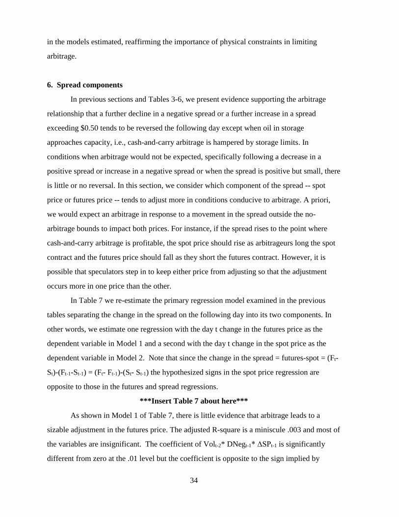
34

in the models estimated, reaffirming the importance of physical constraints in limiting

arbitrage.

6. Spread components

In previous sections and Tables 3-6, we present evidence supporting the arbitrage

relationship that a further decline in a negative spread or a further increase in a spread

exceeding $0.50 tends to be reversed the following day except when oil in storage

approaches capacity, i.e., cash-and-carry arbitrage is hampered by storage limits. In

conditions when arbitrage would not be expected, specifically following a decrease in a

positive spread or increase in a negative spread or when the spread is positive but small, there

is little or no reversal. In this section, we consider which component of the spread -- spot

price or futures price -- tends to adjust more in conditions conducive to arbitrage. A priori,

we would expect an arbitrage in response to a movement in the spread outside the no-

arbitrage bounds to impact both prices. For instance, if the spread rises to the point where

cash-and-carry arbitrage is profitable, the spot price should rise as arbitrageurs long the spot

contract and the futures price should fall as they short the futures contract. However, it is

possible that speculators step in to keep either price from adjusting so that the adjustment

occurs more in one price than the other.

In Table 7 we re-estimate the primary regression model examined in the previous

tables separating the change in the spread on the following day into its two components. In

other words, we estimate one regression with the day t change in the futures price as the

dependent variable in Model 1 and a second with the day t change in the spot price as the

dependent variable in Model 2. Note that since the change in the spread = futures-spot = (Ft-

St)-(Ft-1-St-1) = (Ft- Ft-1)-(St- St-1) the hypothesized signs in the spot price regression are

opposite to those in the futures and spread regressions.

***Insert Table 7 about here***

As shown in Model 1 of Table 7, there is little evidence that arbitrage leads to a

sizable adjustment in the futures price. The adjusted R-square is a miniscule .003 and most of

the variables are insignificant. The coefficient of Volt-2* DNegt-1* ΔSPt-1 is significantly

different from zero at the .01 level but the coefficient is opposite to the sign implied by

35

arbitrage.

In contrast, in Model 2, there is evidence that, in the absence of physical constraints,

the spot price adjusts as implied by arbitrage. Consistent with the expected impact of cash-

and-carry arbitrage, the coefficients of DNegt-1* ΔSPt-1, Volt-2* DNegt-1* ΔSPt-1, and Volt-

2*DPosHight-1* ΔSPt-1 are all significant at the .01 level with the positive signs implied by

arbitrage. The evidence in Table 7 further indicates that as the oil in storage approaches

capacity, this spot price adjustment is impeded since the coefficient of DCap_Utilt-1*

DPosHight-1* ΔSPt-1 is negative and significant. In other words, when storage is not

constrained, a rise in the spread above the upper no-arbitrage limit normally leads to cash-

and-carry arbitrage in which arbitrageurs buy and store oil causing the spot price to rise but

as storage capacity is exhausted this arbitrage is apparently impeded as the spot price does

not rise.34 The adjusted R-square is much smaller than that for the spread regressions in Table

4 but this is to be expected since many non-arbitrage factors tend to impact the spot and

futures prices similarly and thus have much less impact on the spread than on either the spot

or futures prices individually.

In summary, our evidence indicates cash-and-carry arbitrage and reverse cash-and-

carry arbitrage impact the spot price much more than the futures price. In other words, when

the spread rises above, or falls below, the no-arbitrage bounds, it is primarily the spot price

which adjusts to bring the spread back within the bounds. However, when storage levels are

at or near capacity, the spot price adjustment is impeded.

7. Robustness Checks

In the above estimations, we separate DPosLow and DPosHigh at a spread of $0.50.

Also, we use days when storage capacity utilization is in the top 20% of our sample as our

measure of periods when storage is likely constrained. In this section, we examine the

robustness of our results to variations in these measures. Also, since October 2010, the EIA

has provided measures of actual storage capacity at Cushing on a semi-annual basis and we

examine how these more discrete measures of storage capacity utilization affect our results.

34 One of the explanations could be that as storage gets close to its operational capacity, then more oil would be

forced onto the spot market, pushing the spot price lower.

Brennan, Morgan and Justin Solomon, “Cushing, Oklahoma: Small town is holding billions in black gold,”

CNBC, March 7, 2015.

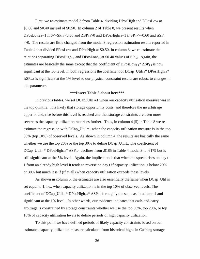
36

First, we re-estimate model 3 from Table 4, dividing DPosHigh and DPosLow at

$0.60 and $0.40 instead of $0.50. In column 2 of Table 8, we present results when

DPosLowt-1=1 if 0<=SPt-2<0.60 and ΔSPt-1>0 and DPosHight-1=1 if SPt-2>=0.60 and ΔSPt-

1>0. The results are little changed from the model 3 regression estimation results reported in

Table 4 that divided PPosLow and DPosHigh at $0.50. In column 3, we re-estimate the

relations separating DPosHight-1 and DPosLowt-1 at $0.40 values of SPt-2. Again, the

estimates are basically the same except that the coefficient of DPosLowt-1* ΔSPt-1 is now

significant at the .05 level. In both regressions the coefficient of DCap_Utilt-1* DPosHight-1*

ΔSPt--1 is significant at the 1% level so our physical constraint results are robust to changes in

this parameter.

***Insert Table 8 about here***

In previous tables, we set DCap_Util =1 when our capacity utilization measure was in

the top quintile. It is likely that storage opportunity costs, and therefore the no arbitrage

upper bound, rise before this level is reached and that storage constraints are even more

severe as the capacity utilization rate rises further. Thus, in column 4 (5) in Table 8 we re-

estimate the regression with DCap_Util =1 when the capacity utilization measure is in the top

30% (top 10%) of observed levels. As shown in column 4, the results are basically the same

whether we use the top 20% or the top 30% to define DCap_UTIL. The coefficient of

DCap_Utilt-1* DPosHight-1* ΔSPt--1 declines from .8185 in Table 4 model 3 to .6179 but is

still significant at the 5% level. Again, the implication is that when the spread rises on day t-

1 from an already high level it tends to reverse on day t if capacity utilization is below 20%

or 30% but much less if (if at all) when capacity utilization exceeds these levels.

As shown in column 5, the estimates are also essentially the same when DCap_Util is

set equal to 1, i.e., when capacity utilization is in the top 10% of observed levels. The

coefficient of DCap_Utilt-1* DPosHight-1* ΔSPt-1 is roughly the same as in column 4 and

significant at the 1% level. In other words, our evidence indicates that cash-and-carry

arbitrage is constrained by storage constraints whether we use the top 30%, top 20%, or top

10% of capacity utilization levels to define periods of high capacity utilization

To this point we have defined periods of likely capacity constraints based on our

estimated capacity utilization measure calculated from historical highs in Cushing storage

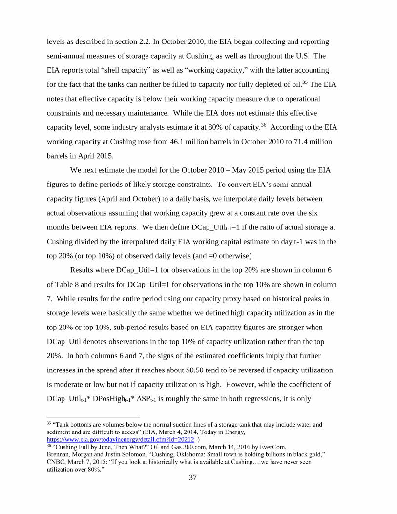
37

levels as described in section 2.2. In October 2010, the EIA began collecting and reporting

semi-annual measures of storage capacity at Cushing, as well as throughout the U.S. The

EIA reports total “shell capacity” as well as “working capacity,” with the latter accounting

for the fact that the tanks can neither be filled to capacity nor fully depleted of oil.35 The EIA

notes that effective capacity is below their working capacity measure due to operational

constraints and necessary maintenance. While the EIA does not estimate this effective

capacity level, some industry analysts estimate it at 80% of capacity.36 According to the EIA

working capacity at Cushing rose from 46.1 million barrels in October 2010 to 71.4 million

barrels in April 2015.

We next estimate the model for the October 2010 – May 2015 period using the EIA

figures to define periods of likely storage constraints. To convert EIA’s semi-annual

capacity figures (April and October) to a daily basis, we interpolate daily levels between

actual observations assuming that working capacity grew at a constant rate over the six

months between EIA reports. We then define DCap_Utilt-1=1 if the ratio of actual storage at

Cushing divided by the interpolated daily EIA working capital estimate on day t-1 was in the

top 20% (or top 10%) of observed daily levels (and =0 otherwise)

Results where DCap_Util=1 for observations in the top 20% are shown in column 6

of Table 8 and results for DCap_Util=1 for observations in the top 10% are shown in column

7. While results for the entire period using our capacity proxy based on historical peaks in

storage levels were basically the same whether we defined high capacity utilization as in the

top 20% or top 10%, sub-period results based on EIA capacity figures are stronger when

DCap_Util denotes observations in the top 10% of capacity utilization rather than the top

20%. In both columns 6 and 7, the signs of the estimated coefficients imply that further

increases in the spread after it reaches about $0.50 tend to be reversed if capacity utilization

is moderate or low but not if capacity utilization is high. However, while the coefficient of

DCap_Utilt-1* DPosHight-1* ΔSPt-1 is roughly the same in both regressions, it is only

35 “Tank bottoms are volumes below the normal suction lines of a storage tank that may include water and

sediment and are difficult to access” (EIA, March 4, 2014, Today in Energy,

https://www.eia.gov/todayinenergy/detail.cfm?id=20212 ) 36 “Cushing Full by June, Then What?” Oil and Gas 360.com, March 14, 2016 by EverCom.

Brennan, Morgan and Justin Solomon, “Cushing, Oklahoma: Small town is holding billions in black gold,”

CNBC, March 7, 2015: “If you look at historically what is available at Cushing….we have never seen

utilization over 80%.”

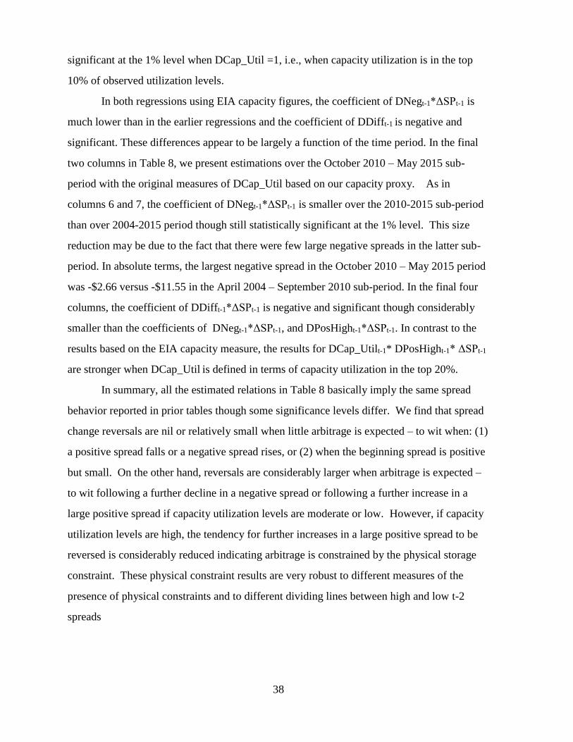
38

significant at the 1% level when DCap_Util =1, i.e., when capacity utilization is in the top

10% of observed utilization levels.

In both regressions using EIA capacity figures, the coefficient of DNegt-1*ΔSPt-1 is

much lower than in the earlier regressions and the coefficient of DDifft-1 is negative and

significant. These differences appear to be largely a function of the time period. In the final

two columns in Table 8, we present estimations over the October 2010 – May 2015 sub-

period with the original measures of DCap_Util based on our capacity proxy. As in

columns 6 and 7, the coefficient of DNegt-1*ΔSPt-1 is smaller over the 2010-2015 sub-period

than over 2004-2015 period though still statistically significant at the 1% level. This size

reduction may be due to the fact that there were few large negative spreads in the latter sub-

period. In absolute terms, the largest negative spread in the October 2010 – May 2015 period

was -$2.66 versus -$11.55 in the April 2004 – September 2010 sub-period. In the final four

columns, the coefficient of DDifft-1*ΔSPt-1 is negative and significant though considerably

smaller than the coefficients of DNegt-1*ΔSPt-1, and DPosHight-1*ΔSPt-1. In contrast to the

results based on the EIA capacity measure, the results for DCap_Utilt-1* DPosHight-1* ΔSPt-1

are stronger when DCap_Util is defined in terms of capacity utilization in the top 20%.

In summary, all the estimated relations in Table 8 basically imply the same spread

behavior reported in prior tables though some significance levels differ. We find that spread

change reversals are nil or relatively small when little arbitrage is expected – to wit when: (1)

a positive spread falls or a negative spread rises, or (2) when the beginning spread is positive

but small. On the other hand, reversals are considerably larger when arbitrage is expected –

to wit following a further decline in a negative spread or following a further increase in a

large positive spread if capacity utilization levels are moderate or low. However, if capacity

utilization levels are high, the tendency for further increases in a large positive spread to be

reversed is considerably reduced indicating arbitrage is constrained by the physical storage

constraint. These physical constraint results are very robust to different measures of the

presence of physical constraints and to different dividing lines between high and low t-2

spreads

39

8. Conclusions

While there is considerable evidence in the literature documenting the effects of

financial constraints on arbitrage and pricing, there is considerably less attention paid to

physical constraints, which can be equally important when the value of financial securities is

derived from physical assets. We extend the literature by studying the effect of crude oil

storage constraints on arbitrage activity in the U.S. crude oil market. We find that when

actual crude oil storage levels are well short of available storage capacity, the behavior of the

crude futures-spot spread is consistent with arbitrage returning the spread to within

unobservable no-arbitrage bounds – albeit with a lag. When arbitrage appears unlikely – i.e.,

when a positive spread declines or a negative spread rises or when the beginning spread is

small – the change in the spread on day t is basically uncorrelated with the change in the

spread on day t-1. However, when arbitrage appears more likely – i.e., when an already

negative spread declines further on day t-1 or a large positive spread increases more on day t-

1 -- the change on day t is strongly negatively correlated with the change on day t-1 as one

would expect if the arbitrage is pulling the spread back within no-arbitrage bounds. This

spread change reversal is even stronger when volatility is high. In summary, we observe

strong negative autocorrelations in the futures spot spread when the arbitrage hypothesis

predicts we should, and little or no autocorrelation when the arbitrage hypothesis predicts we

should. The fact that these autocorrelations are observable in daily data is consistent with

arbitrageurs often needing time to contract for storage at the hub. Interestingly, the evidence

indicates that the spot price adjusts more than the futures price to bring the spread back

within no-arbitrage bounds suggesting that the futures price is set more by speculators and

other traders.

In contrast, when storage levels approach full capacity, further increases in an already

large positive crude oil spread on day t-1 do not tend to be reversed on day t, or are reduced

much less than when storage is plentiful. Thus, our evidence indicates that while normally

cash-and-carry arbitrage operates to return the futures-spot spread to within the no-arbitrage

upper bound, this breaks down in periods of very high capacity utilization. On the other

hand, we find little evidence that oil inventories are ever so low as to interfere with reverse

cash-and-carry arbitrage. We further find evidence that financial constraints also hindered

40

arbitrage in the crude oil market over our sample period. Nonetheless, our physical

constraint results are robust to accounting for possible financial constraints as well as to

different measures of when physical constraints are likely operative. Our findings highlight

the importance of accounting for physical arbitrage limits in the pricing of commodity

futures, and also contribute to the Theory of Storage literature by highlighting the

consequences when inventories approach storage capacity limits.

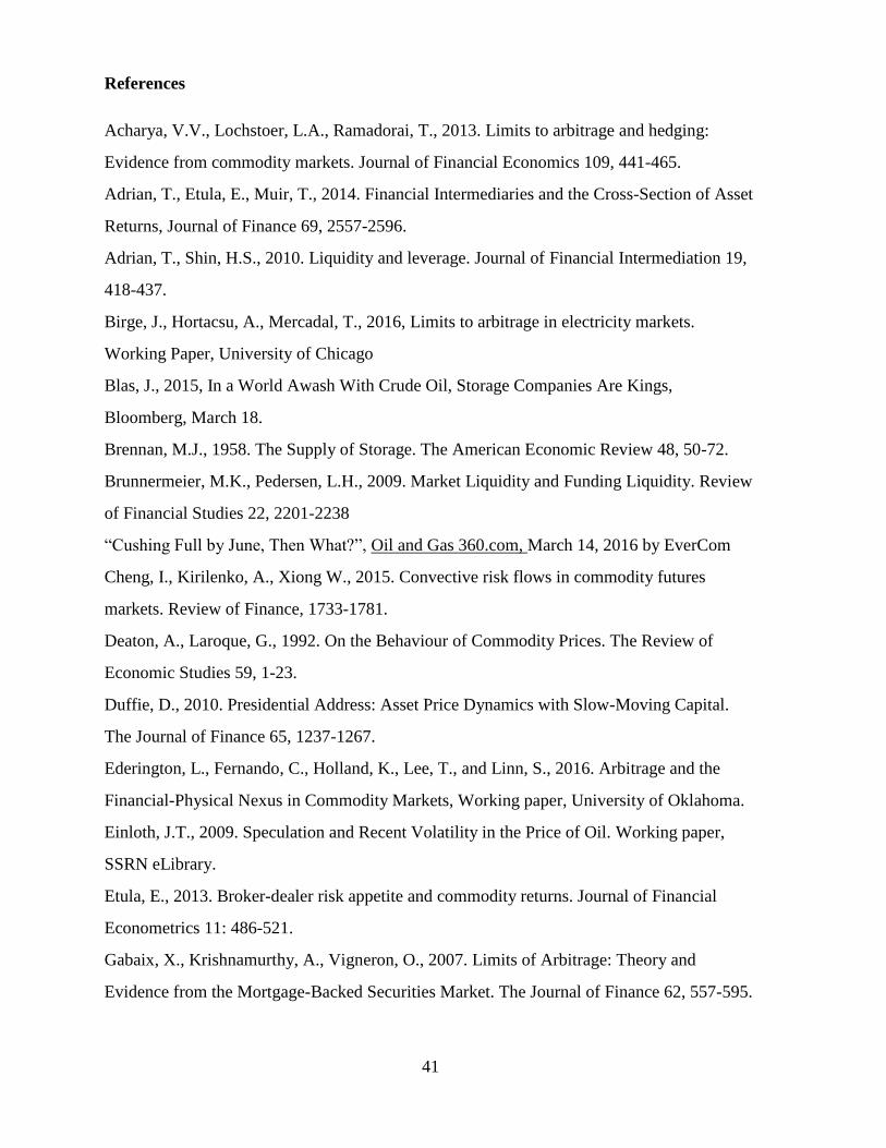
41

References

Acharya, V.V., Lochstoer, L.A., Ramadorai, T., 2013. Limits to arbitrage and hedging:

Evidence from commodity markets. Journal of Financial Economics 109, 441-465.

Adrian, T., Etula, E., Muir, T., 2014. Financial Intermediaries and the Cross-Section of Asset

Returns, Journal of Finance 69, 2557-2596.

Adrian, T., Shin, H.S., 2010. Liquidity and leverage. Journal of Financial Intermediation 19,

418-437.

Birge, J., Hortacsu, A., Mercadal, T., 2016, Limits to arbitrage in electricity markets.

Working Paper, University of Chicago

Blas, J., 2015, In a World Awash With Crude Oil, Storage Companies Are Kings,

Bloomberg, March 18.

Brennan, M.J., 1958. The Supply of Storage. The American Economic Review 48, 50-72.

Brunnermeier, M.K., Pedersen, L.H., 2009. Market Liquidity and Funding Liquidity. Review

of Financial Studies 22, 2201-2238

“Cushing Full by June, Then What?”, Oil and Gas 360.com, March 14, 2016 by EverCom

Cheng, I., Kirilenko, A., Xiong W., 2015. Convective risk flows in commodity futures

markets. Review of Finance, 1733-1781.

Deaton, A., Laroque, G., 1992. On the Behaviour of Commodity Prices. The Review of

Economic Studies 59, 1-23.

Duffie, D., 2010. Presidential Address: Asset Price Dynamics with Slow-Moving Capital.

The Journal of Finance 65, 1237-1267.

Ederington, L., Fernando, C., Holland, K., Lee, T., and Linn, S., 2016. Arbitrage and the

Financial-Physical Nexus in Commodity Markets, Working paper, University of Oklahoma.

Einloth, J.T., 2009. Speculation and Recent Volatility in the Price of Oil. Working paper,

SSRN eLibrary.

Etula, E., 2013. Broker-dealer risk appetite and commodity returns. Journal of Financial

Econometrics 11: 486-521.

Gabaix, X., Krishnamurthy, A., Vigneron, O., 2007. Limits of Arbitrage: Theory and

Evidence from the Mortgage-Backed Securities Market. The Journal of Finance 62, 557-595.

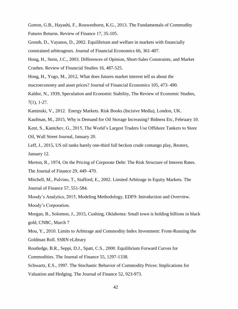
42

Gorton, G.B., Hayashi, F., Rouwenhorst, K.G., 2013. The Fundamentals of Commodity

Futures Returns. Review of Finance 17, 35-105.

Gromb, D., Vayanos, D., 2002. Equilibrium and welfare in markets with financially

constrained arbitrageurs. Journal of Financial Economics 66, 361-407.

Hong, H., Stein, J.C., 2003. Differences of Opinion, Short-Sales Constraints, and Market

Crashes. Review of Financial Studies 16, 487-525.

Hong, H., Yogo, M., 2012, What does futures market interest tell us about the

macroeconomy and asset prices? Journal of Financial Economics 105, 473–490.

Kaldor, N., 1939, Speculation and Economic Stability, The Review of Economic Studies,

7(1), 1-27.

Kaminski, V., 2012. Energy Markets. Risk Books (Incisive Media), London, UK.

Kaufman, M., 2015, Why is Demand for Oil Storage Increasing? Bidness Etc, February 10.

Kent, S., Kantchev, G., 2015, The World’s Largest Traders Use Offshore Tankers to Store

Oil, Wall Street Journal, January 20.

Leff, J., 2015, US oil tanks barely one-third full beckon crude contango play, Reuters,

January 12.

Merton, R., 1974, On the Pricing of Corporate Debt: The Risk Structure of Interest Rates.

The Journal of Finance 29, 449–470.

Mitchell, M., Pulvino, T., Stafford, E., 2002. Limited Arbitrage in Equity Markets. The

Journal of Finance 57, 551-584.

Moody’s Analytics, 2015, Modeling Methodology, EDF9: Introduction and Overview.

Moody’s Corporation.

Morgan, B., Solomon, J., 2015, Cushing, Oklahoma: Small town is holding billions in black

gold, CNBC, March 7

Mou, Y., 2010. Limits to Arbitrage and Commodity Index Investment: Front-Running the

Goldman Roll. SSRN eLibrary

Routledge, B.R., Seppi, D.J., Spatt, C.S., 2000. Equilibrium Forward Curves for

Commodities. The Journal of Finance 55, 1297-1338.

Schwartz, E.S., 1997. The Stochastic Behavior of Commodity Prices: Implications for

Valuation and Hedging. The Journal of Finance 52, 923-973.

43

Shleifer, A. and R. W. Vishny, 1997, The Limits of Arbitrage, Journal of Finance 52: 35-55.

Working, H., 1949. The Theory of Price of Storage. American Economic Review 39, 1254-

1262.

Zmijewski, M. E., 1984, Methodological Issues Related to the Estimation of Financial

Distress Prediction Models, Journal of Accounting Research, Supplement, 59-82.

44

9.2

9.6

10.0

10.4

10.8

11.2

04 05 06 07 08 09 10 11 12 13 14 15

Effective Capacity at Cushing, OK (estimate) - logarithmic scaleStorage at Cushing, OK (actual) - logarithmic scale

Year, 20xx

Figure 1 – Estimated Storage Capacity and Actual Storage at Cushing (April 2004-April 2015)

This figure presents the actual weekly crude oil storage and estimated effective crude oil capacity

from April 2004 to April 2015 at Cushing, Oklahoma, which is the NYMEX physical settlement

point for the crude oil WTI future contract. Crude oil storage data is collected from the U.S. Energy

Information Administration (EIA). The estimation of the proxy for effective storage capacity is

described in section 2.2.

45

$-2.00

$-1.00

$0.00

$1.00

$2.00

$3.00

$4.00

$5.00

$6.00

0.3

0.4

0.5

0.6

0.7

0.8

0.9

1.0

1.1

04 05 06 07 08 09 10 11 12 13 14 15

Future-Spot Spread (10 day moving average)

Capacity Utilization at Cushing, OK (10 day moving average)

Year, 20xx

Ca

pa

city

Utiliz

atio

n

Fu

ture

-Sp

ot

Sp

rea

d (

$)

Figure 2 – Cushing, OK Capacity Utilization and the Crude Oil WTI Future-Spot Spread (10-

day moving averages) (April 2004-April 2015)

This figure presents the 10-day moving averages of both the future-spot spread and the capacity

utilization at Cushing, OK from April 2004 to April 2015. Capacity utilization is measured as the

ratio of the actual level of crude oil stocks as reported by the EIA to the proxy for effective storage

capacity. The futures-spot spread is the difference between the price of the second and nearby WTI

crude oil futures contracts.

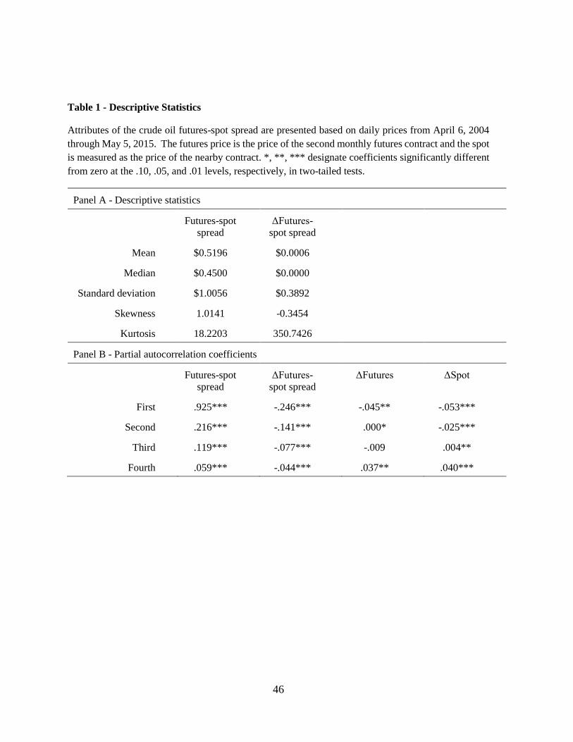
46

Table 1 - Descriptive Statistics

Attributes of the crude oil futures-spot spread are presented based on daily prices from April 6, 2004

through May 5, 2015. The futures price is the price of the second monthly futures contract and the spot

is measured as the price of the nearby contract. *, **, *** designate coefficients significantly different

from zero at the .10, .05, and .01 levels, respectively, in two-tailed tests.

Panel A - Descriptive statistics

Futures-spot

spread

ΔFutures-

spot spread

Mean $0.5196 $0.0006

Median $0.4500 $0.0000

Standard deviation $1.0056 $0.3892

Skewness 1.0141 -0.3454

Kurtosis 18.2203 350.7426

Panel B - Partial autocorrelation coefficients

Futures-spot

spread

ΔFutures-

spot spread

ΔFutures ΔSpot

First .925*** -.246*** -.045** -.053***

Second .216*** -.141*** .000* -.025***

Third .119*** -.077*** -.009 .004**

Fourth .059*** -.044*** .037** .040***

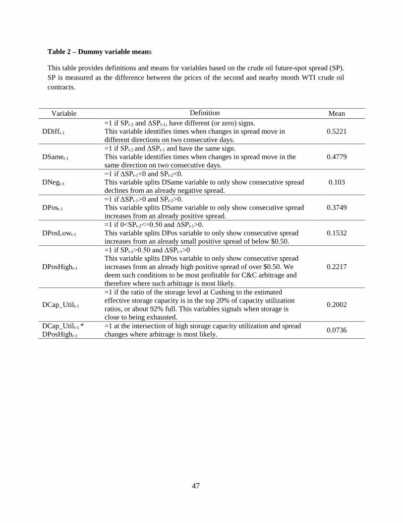
47

Table 2 – Dummy variable means

This table provides definitions and means for variables based on the crude oil future-spot spread (SP).

SP is measured as the difference between the prices of the second and nearby month WTI crude oil

contracts.

Variable Definition Mean

DDifft-1

=1 if SPt-2 and ΔSPt-1, have different (or zero) signs.

This variable identifies times when changes in spread move in

different directions on two consecutive days.

0.5221

DSamet-1

=1 if SPt-2 and ΔSPt-1 and have the same sign.

This variable identifies times when changes in spread move in the

same direction on two consecutive days.

0.4779

DNegt-1

=1 if ΔSPt-1<0 and SPt-2<0.

This variable splits DSame variable to only show consecutive spread

declines from an already negative spread.

0.103

DPost-1

=1 if ΔSPt-1>0 and SPt-2>0.

This variable splits DSame variable to only show consecutive spread

increases from an already positive spread.

0.3749

DPosLowt-1

=1 if 0<SPt-2<=0.50 and ΔSPt-1>0.

This variable splits DPos variable to only show consecutive spread

increases from an already small positive spread of below $0.50.

0.1532

DPosHight-1

=1 if SPt-2>0.50 and ΔSPt-1>0

This variable splits DPos variable to only show consecutive spread

increases from an already high positive spread of over $0.50. We

deem such conditions to be most profitable for C&C arbitrage and

therefore where such arbitrage is most likely.

0.2217

DCap_Utilt-1

=1 if the ratio of the storage level at Cushing to the estimated

effective storage capacity is in the top 20% of capacity utilization

ratios, or about 92% full. This variables signals when storage is

close to being exhausted.

0.2002

DCap_Utilt-1 *

DPosHight-1

=1 at the intersection of high storage capacity utilization and spread

changes where arbitrage is most likely. 0.0736

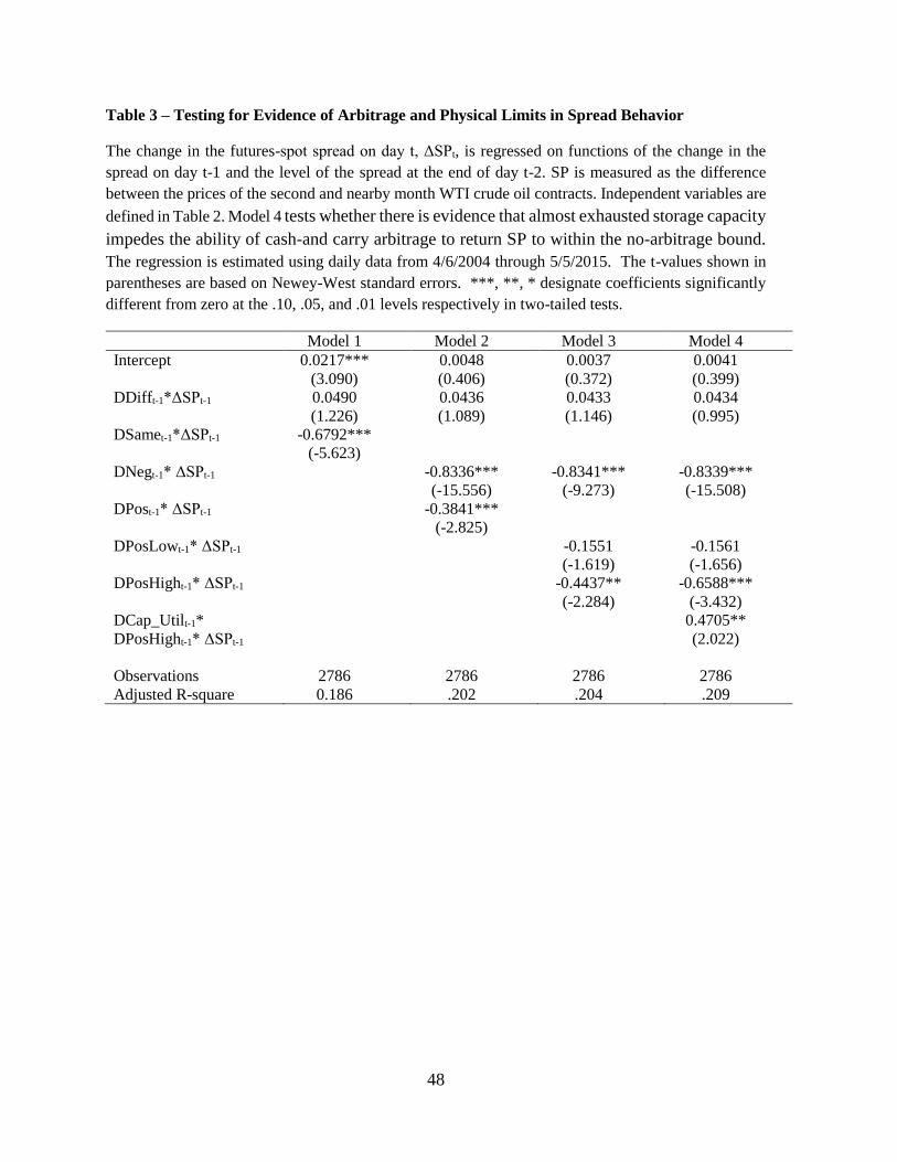
48

Table 3 – Testing for Evidence of Arbitrage and Physical Limits in Spread Behavior

The change in the futures-spot spread on day t, ΔSPt, is regressed on functions of the change in the

spread on day t-1 and the level of the spread at the end of day t-2. SP is measured as the difference

between the prices of the second and nearby month WTI crude oil contracts. Independent variables are

defined in Table 2. Model 4 tests whether there is evidence that almost exhausted storage capacity

impedes the ability of cash-and carry arbitrage to return SP to within the no-arbitrage bound.

The regression is estimated using daily data from 4/6/2004 through 5/5/2015. The t-values shown in

parentheses are based on Newey-West standard errors. ***, **, * designate coefficients significantly

different from zero at the .10, .05, and .01 levels respectively in two-tailed tests.

Model 1 Model 2 Model 3 Model 4

Intercept 0.0217***

(3.090)

0.0048

(0.406)

0.0037

(0.372)

0.0041

(0.399)

DDifft-1*ΔSPt-1 0.0490

(1.226)

0.0436

(1.089)

0.0433

(1.146)

0.0434

(0.995)

DSamet-1*ΔSPt-1 -0.6792***

(-5.623)

DNegt-1* ΔSPt-1

-0.8336***

(-15.556)

-0.8341***

(-9.273)

-0.8339***

(-15.508)

DPost-1* ΔSPt-1

-0.3841***

(-2.825)

DPosLowt-1* ΔSPt-1

-0.1551

(-1.619)

-0.1561

(-1.656)

DPosHight-1* ΔSPt-1

-0.4437**

(-2.284)

-0.6588***

(-3.432)

DCap_Utilt-1*

DPosHight-1* ΔSPt-1

0.4705**

(2.022)

Observations 2786 2786 2786 2786

Adjusted R-square 0.186 .202 .204 .209

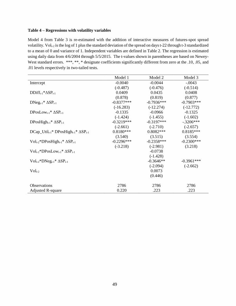
49

Table 4 – Regressions with volatility variables

Model 4 from Table 3 is re-estimated with the addition of interactive measures of futures-spot spread

volatility. Volt-2 is the log of 1 plus the standard deviation of the spread on days t-22 through t-3 standardized

to a mean of 0 and variance of 1. Independent variables are defined in Table 2. The regression is estimated

using daily data from 4/6/2004 through 5/5/2015. The t-values shown in parentheses are based on Newey-

West standard errors. ***, **, * designate coefficients significantly different from zero at the .10, .05, and

.01 levels respectively in two-tailed tests.

Model 1 Model 2 Model 3

Intercept -0.0040

(-0.487)

-0.0044

(-0.476)

-.0043

(-0.514)

DDifft-1*ΔSPt-1

0.0409

(0.878)

0.0435

(0.819)

0.0408

(0.877)

DNegt-1* ΔSPt-1 -0.8377***

(-16.283)

-0.7936***

(-12.274)

-0.7903***

(-12.772)

DPosLowt-1* ΔSPt-1

-0.1335

(-1.424)

-0.0966

(-1.455)

-0.1325

(-1.602)

DPosHight-1* ΔSPt-1 -0.3219***

(-2.661)

-0.3197***

(-2.710)

-.3206***

(-2.657)

DCap_Utilt-1* DPosHight-1* ΔSPt-1 0.8180***

(3.540)

0.8082***

(3.515)

0.8185***

(3.554)

Volt-2*DPosHight-1* ΔSPt-1

-0.2296***

(-3.218)

-0.2358***

(-2.981)

-0.2300***

(3.218)

Volt-2*DPosLowt-1* ΔSPt-1

-0.0738

(-1.428)

Volt-2*DNegt-1* ΔSPt-1

-0.3646**

(-2.094)

-0.3961***

(-2.662)

Volt-2

0.0073

(0.446)

Observations 2786 2786 2786

Adjusted R-square 0.220 .223 .223

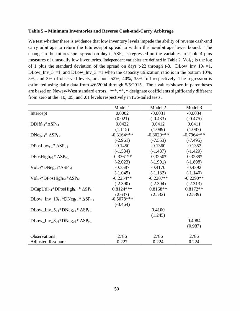
50

Table 5 – Minimum Inventories and Reverse Cash-and-Carry Arbitrage

We test whether there is evidence that low inventory levels impede the ability of reverse cash-and

carry arbitrage to return the futures-spot spread to within the no-arbitrage lower bound. The

change in the futures-spot spread on day t, ΔSPt, is regressed on the variables in Table 4 plus

measures of unusually low inventories. Independent variables are defined in Table 2. Volt-2 is the log

of 1 plus the standard deviation of the spread on days t-22 through t-3. DLow_Inv_10t =1,

DLow_Inv_5t =1, and DLow_Inv_3t =1 when the capacity utilization ratio is in the bottom 10%,

5%, and 3% of observed levels, or about 52%, 40%, 35% full respectively. The regression is

estimated using daily data from 4/6/2004 through 5/5/2015. The t-values shown in parentheses

are based on Newey-West standard errors. ***, **, * designate coefficients significantly different

from zero at the .10, .05, and .01 levels respectively in two-tailed tests.

Model 1 Model 2 Model 3

Intercept 0.0002

(0.021)

-0.0031

(-0.433)

-0.0034

(-0.475)

DDifft-1*ΔSPt-1 0.0422

(1.115)

0.0412

(1.089)

0.0411

(1.087)

DNegt-1* ΔSPt-1 -0.3164***

(-2.961)

-0.8020***

(-7.553)

-0.7964***

(-7.495)

DPosLowt-1* ΔSPt-1 -0.1450

(-1.534)

-0.1360

(-1.437)

-0.1352

(-1.429)

DPosHight-1* ΔSPt-1

Volt-2*DNegt-1*ΔSPt-1

Volt-2*DPosHight-1*ΔSPt-1

-0.3361**

(-2.023)

-0.3587

(-1.045)

-0.2254**

(-2.390)

-0.3250*

(-1.901)

-0.4170

(-1.132)

-0.2287**

(-2.304)

-0.3239*

(-1.898)

-0.4392

(-1.140)

-0.2290**

(-2.313)

DCapUtilt-1*DPosHight-1 * ΔSPt-1 0.8124***

(2.637)

0.8168**

(2.532)

0.8172**

(2.539)

DLow_Inv_10t-1*DNegt-1* ΔSPt-1 -0.5078***

(-3.464)

DLow_Inv_5t-1*DNegt-1* ΔSPt-1 0.4100

(1.245)

DLow_Inv_3t-1*DNegt-1* ΔSPt-1

0.4084

(0.987)

Observations 2786 2786 2786

Adjusted R-square 0.227 0.224 0.224

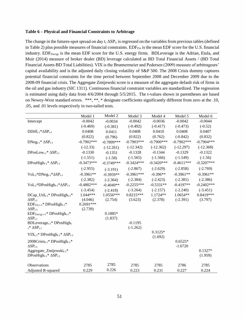
51

Table 6 – Physical and Financial Constraints to Arbitrage

The change in the futures-spot spread on day t, ΔSPt, is regressed on the variables from previous tables (defined

in Table 2) plus possible measures of financial constraints. EDFFin is the mean EDF score for the U.S. financial

industry. EDFEnergy is the mean EDF score for the U.S. energy firms. BDLeverage is the Adrian, Etula, and

Muir (2014) measure of broker dealer (BD) leverage calculated as BD Total Financial Assets / (BD Total

Financial Assets-BD Total Liabilities). VIX is the Brunnermeier and Pedersen (2009) measure of arbitrageurs’

capital availability and is the adjusted daily closing volatility of S&P 500. The 2008 Crisis dummy captures

potential financial constraints for the time period between September 2008 and December 2009 due to the

2008-09 financial crisis. The Aggregate Zmijewski score is a measure of the aggregate default risk of firms in

the oil and gas industry (SIC 1311). Continuous financial constraint variables are standardized. The regression

is estimated using daily data from 4/6/2004 through 5/5/2015. The t-values shown in parentheses are based

on Newey-West standard errors. ***, **, * designate coefficients significantly different from zero at the .10,

.05, and .01 levels respectively in two-tailed tests.

Model 1 Model 2 Model 3 Model 4 Model 5 Model 6

Intercept -0.0042 -0.0034 -0.0042 -0.0036 -0.0042 -0.0044

(-0.469) (-0.381) (-0.492) (-0.417) (-0.473) (-0.52)

DDifft-1*ΔSPt-1 0.0408 0.0411 0.0408 0.0410 0.0408 0.0407

(0.822) (0.796) (0.822) (0.762) (-0.842) (0.832)

DNegt-1* ΔSPt-1 -0.7902*** -0.7899*** -0.7903*** -0.7900*** -0.7902*** -0.7904***

(-12.33) (-12.261) (-12.342) (-12.362) (-12.297) (-12.368)

DPosLowt-1* ΔSPt-1 -0.1330 -0.1351 -0.1328 -0.1344 -0.1329 -0.1322

(-1.551) (-1.58) (-1.565) (-1.566) (-1.549) (-1.56)

DPosHight-1* ΔSPt-1 -0.3473*** -0.3749*** -0.3424*** -0.3420*** -0.4611*** -0.3207***

(-2.955) (-3.191) (-2.867) (-2.629) (-2.858) (-2.769)

Volt-2*DNegt-1*ΔSPt-1 -0.3961** -0.3959** -0.3961*** -0.396** -0.3961** -0.3961**

(-2.382) (-2.364) (-2.384) (-2.423) (-2.381) (-2.386)

Volt-2*DPosHight-1*ΔSPt-1 -0.4882*** -0.4049** -0.2255*** -0.5331** -0.4197** -0.2402***

(-3.454) (-2.418) (-3.264) (-2.157) (-2.240) (-3.451)

DCap_Utilt-1* DPosHight-1*

ΔSPt-1

1.044***

(4.046)

1.0556***

(2.754)

0.8215***

(3.623)

1.1724**

(2.378)

1.0654**

(-2.391)

0.8419***

(3.797)

EDFFin t-1* DPosHight-1*

ΔSPt-1

0.2691***

(2.739)

EDFEnergy t-1* DPosHight-1*

ΔSPt-1

0.1885*

(1.837)

BDLeveraget-1* DPosHight-

1* ΔSPt-1

-0.1195

(-1.262)

VIXt-1* DPosHight-1* ΔSPt-1 0.3125*

(1.692)

2008Crisist-1* DPosHight-1*

ΔSPt-1

0.6525*

-1.6720

Aggregate_Zmijewskit-1*

DPosHight-1* ΔSPt-1

0.1327*

(1.959)

Observations 2785 2785 2785 2785 2786 2785

Adjusted R-squared 0.229 0.226 0.223 0.231 0.227 0.224

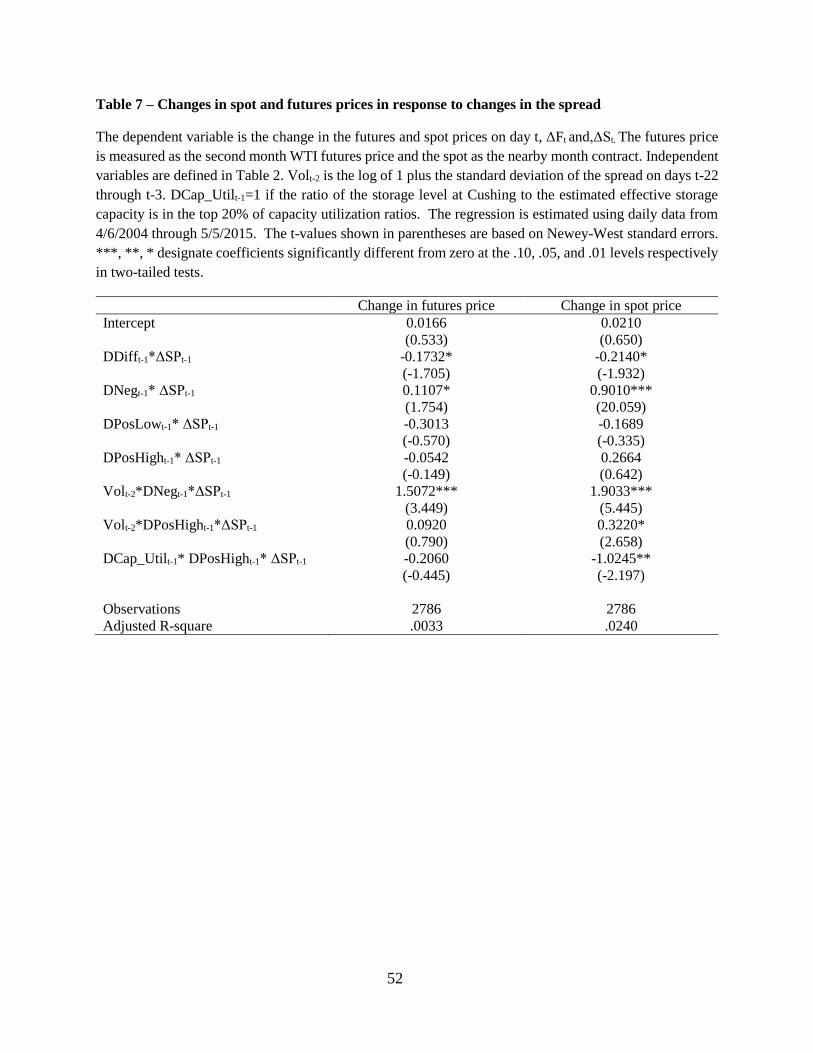
52

Table 7 – Changes in spot and futures prices in response to changes in the spread

The dependent variable is the change in the futures and spot prices on day t, ΔFt and,ΔSt. The futures price

is measured as the second month WTI futures price and the spot as the nearby month contract. Independent

variables are defined in Table 2. Volt-2 is the log of 1 plus the standard deviation of the spread on days t-22

through t-3. DCap_Utilt-1=1 if the ratio of the storage level at Cushing to the estimated effective storage

capacity is in the top 20% of capacity utilization ratios. The regression is estimated using daily data from

4/6/2004 through 5/5/2015. The t-values shown in parentheses are based on Newey-West standard errors.

***, **, * designate coefficients significantly different from zero at the .10, .05, and .01 levels respectively

in two-tailed tests.

Change in futures price Change in spot price

Intercept 0.0166

(0.533)

0.0210

(0.650)

DDifft-1*ΔSPt-1 -0.1732*

(-1.705)

-0.2140*

(-1.932)

DNegt-1* ΔSPt-1 0.1107*

(1.754)

0.9010***

(20.059)

DPosLowt-1* ΔSPt-1 -0.3013

(-0.570)

-0.1689

(-0.335)

DPosHight-1* ΔSPt-1

Volt-2*DNegt-1*ΔSPt-1

Volt-2*DPosHight-1*ΔSPt-1

-0.0542

(-0.149)

1.5072***

(3.449)

0.0920

(0.790)

0.2664

(0.642)

1.9033***

(5.445)

0.3220*

(2.658)

DCap_Utilt-1* DPosHight-1* ΔSPt-1 -0.2060

(-0.445)

-1.0245**

(-2.197)

Observations 2786 2786

Adjusted R-square .0033 .0240

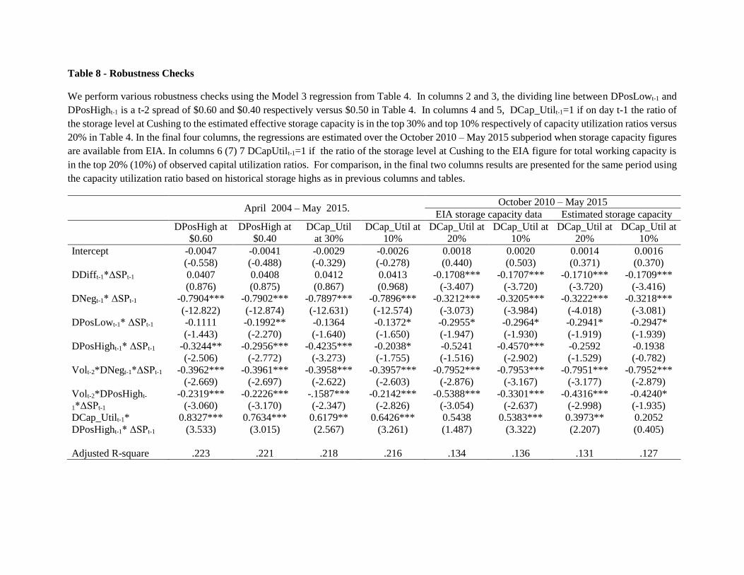
Table 8 - Robustness Checks

We perform various robustness checks using the Model 3 regression from Table 4. In columns 2 and 3, the dividing line between DPosLowt-1 and

DPosHight-1 is a t-2 spread of $0.60 and $0.40 respectively versus $0.50 in Table 4. In columns 4 and 5, DCap_Utilt-1=1 if on day t-1 the ratio of

the storage level at Cushing to the estimated effective storage capacity is in the top 30% and top 10% respectively of capacity utilization ratios versus

20% in Table 4. In the final four columns, the regressions are estimated over the October 2010 – May 2015 subperiod when storage capacity figures

are available from EIA. In columns 6 (7) 7 DCapUtilt-1=1 if the ratio of the storage level at Cushing to the EIA figure for total working capacity is

in the top 20% (10%) of observed capital utilization ratios. For comparison, in the final two columns results are presented for the same period using

the capacity utilization ratio based on historical storage highs as in previous columns and tables.

April 2004 – May 2015.

October 2010 – May 2015

EIA storage capacity data Estimated storage capacity

DPosHigh at

$0.60

DPosHigh at

$0.40

DCap_Util

at 30%

DCap_Util at

10%

DCap_Util at

20%

DCap_Util at

10%

DCap_Util at

20%

DCap_Util at

10%

Intercept -0.0047

(-0.558)

-0.0041

(-0.488)

-0.0029

(-0.329)

-0.0026

(-0.278)

0.0018

(0.440)

0.0020

(0.503)

0.0014

(0.371)

0.0016

(0.370)

DDifft-1*ΔSPt-1 0.0407

(0.876)

0.0408

(0.875)

0.0412

(0.867)

0.0413

(0.968)

-0.1708***

(-3.407)

-0.1707***

(-3.720)

-0.1710***

(-3.720)

-0.1709***

(-3.416)

DNegt-1* ΔSPt-1 -0.7904***

(-12.822)

-0.7902***

(-12.874)

-0.7897***

(-12.631)

-0.7896***

(-12.574)

-0.3212***

(-3.073)

-0.3205***

(-3.984)

-0.3222***

(-4.018)

-0.3218***

(-3.081)

DPosLowt-1* ΔSPt-1 -0.1111

(-1.443)

-0.1992**

(-2.270)

-0.1364

(-1.640)

-0.1372*

(-1.650)

-0.2955*

(-1.947)

-0.2964*

(-1.930)

-0.2941*

(-1.919)

-0.2947*

(-1.939)

DPosHight-1* ΔSPt-1 -0.3244**

(-2.506)

-0.2956***

(-2.772)

-0.4235***

(-3.273)

-0.2038*

(-1.755)

-0.5241

(-1.516)

-0.4570***

(-2.902)

-0.2592

(-1.529)

-0.1938

(-0.782)

Volt-2*DNegt-1*ΔSPt-1

-0.3962***

(-2.669)

-0.3961***

(-2.697)

-0.3958***

(-2.622)

-0.3957***

(-2.603)

-0.7952***

(-2.876)

-0.7953***

(-3.167)

-0.7951***

(-3.177)

-0.7952***

(-2.879)

Volt-2*DPosHight-

1*ΔSPt-1

-0.2319***

(-3.060)

-0.2226***

(-3.170)

-.1587***

(-2.347)

-0.2142***

(-2.826)

-0.5388***

(-3.054)

-0.3301***

(-2.637)

-0.4316***

(-2.998)

-0.4240*

(-1.935)

DCap_Utilt-1*

DPosHight-1* ΔSPt-1

0.8327***

(3.533)

0.7634***

(3.015)

0.6179**

(2.567)

0.6426***

(3.261)

0.5438

(1.487)

0.5383***

(3.322)

0.3973**

(2.207)

0.2052

(0.405)

Adjusted R-square .223 .221 .218 .216 .134 .136 .131 .127