AR5 SOD Chapter 18

Do Not Cite, Quote or Distribute

Working Group III – Mitigation of Climate Change

Annex II

Metrics and Methodology

Second Order Draft (SOD) IPCC WG III AR5

Do Not Cite, Quote or Distribute 1 of 35 Annex II WGIII_AR5_Draft2_AnnexII 20 February 2013

Chapter: Annex II

Title: Methods and Metrics

(Sub)Section: All

Author(s): CLAs: Volker Krey, Omar Masera, Michael Hanemann

LAs: Geoffrey Blanford, Thomas Bruckner, Roger Cooke, Helmut Haberl, Edgar Hertwich, Elmar Kriegler, Daniel Mueller, Sergey Paltsev, Diana Ürge-Vorsatz

CAs: Dominique Van Der Mensbrugghe

Remarks: Second Order Draft (SOD)

Version: 1

File name: WGIII_AR5_Draft2_AnnexII.doc

Date: 20 February 2013 Template Version: 5

1

Table of changes 2

No Date Version Place Description Editor

1 TT.MM.JJJJ 01 initial Version

3

Turquoise highlights are inserted comments from Authors or TSU i.e. [AUTHORS/TSU: ….] 4

5



Annex II: Methods and Metrics 1

Contents 2

Annex II: Methods and Metrics ............................................................................................................... 2 3

A.II.1 Standard units and unit conversion .......................................................................................... 3 4

A.II.1.1 Standard units .................................................................................................................... 3 5

A.II.1.2 Physical unit conversion ..................................................................................................... 4 6

A.II.1.3 Monetary unit conversion ................................................................................................. 5 7

A.II.2 Costs Metrics ............................................................................................................................. 6 8

A.II.2.1 Levelised costs ................................................................................................................... 6 9

A.II.2.1.1 Concept, methodology and levelised costs of energy ................................................ 6 10

A.II.2.1.2 Levelised costs of conserved energy .......................................................................... 8 11

A.II.2.2 Mitigation cost metrics ...................................................................................................... 9 12

A.II.3 Primary energy accounting ....................................................................................................... 9 13

A.II.4 Carbon footprinting, lifecycle assessment, material flow analysis ......................................... 12 14

A.II.4.1 Material flow analysis ...................................................................................................... 12 15

A.II.4.2 Carbon footprinting and input-output analysis ............................................................... 13 16

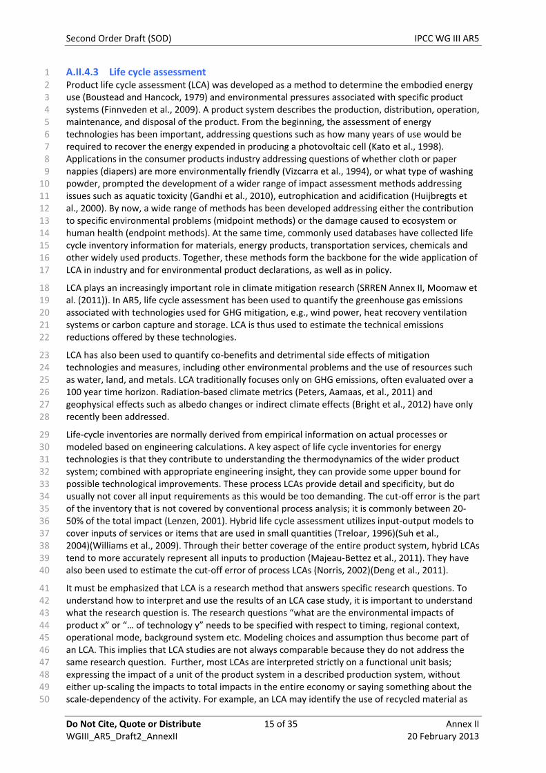
A.II.4.3 Life cycle assessment ....................................................................................................... 15 17

A.II.5 Fat Tailed Distributions ........................................................................................................... 16 18

A.II.6 Region Definitions ................................................................................................................... 18 19

A.II.6.1 RCP5 ................................................................................................................................. 19 20

A.II.6.2 RCP10 ............................................................................................................................... 20 21

A.II.6.3 ECON5 (Economy-based Aggregation) ............................................................................ 20 22

A.II.7 Mapping of Emission Sources to Sectors ................................................................................ 21 23

A.II.7.2 Energy .............................................................................................................................. 22 24

A.II.7.3 Transport .......................................................................................................................... 22 25

A.II.7.4 Buildings ........................................................................................................................... 23 26

A.II.7.5 Industry ............................................................................................................................ 24 27

A.II.7.6 AFOLU .............................................................................................................................. 25 28

29

30



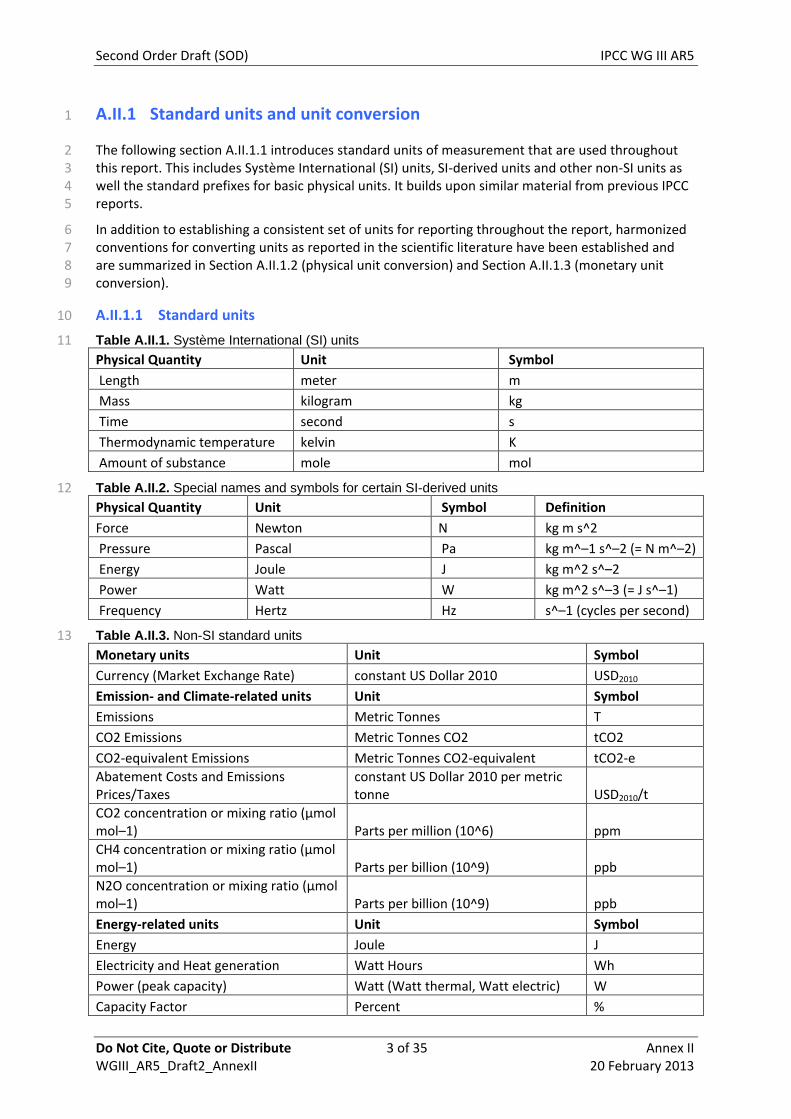
A.II.1 Standard units and unit conversion 1

The following section A.II.1.1 introduces standard units of measurement that are used throughout 2 this report. This includes Système International (SI) units, SI-derived units and other non-SI units as 3 well the standard prefixes for basic physical units. It builds upon similar material from previous IPCC 4 reports. 5

In addition to establishing a consistent set of units for reporting throughout the report, harmonized 6 conventions for converting units as reported in the scientific literature have been established and 7 are summarized in Section A.II.1.2 (physical unit conversion) and Section A.II.1.3 (monetary unit 8 conversion). 9

A.II.1.1 Standard units 10

Table A.II.1. Système International (SI) units 11

Physical Quantity Unit Symbol

Length meter m

Mass kilogram kg

Time second s

Thermodynamic temperature kelvin K

Amount of substance mole mol

Table A.II.2. Special names and symbols for certain SI-derived units 12

Physical Quantity Unit Symbol Definition

Force Newton N kg m s^2

Pressure Pascal Pa kg m^–1 s^–2 (= N m^–2)

Energy Joule J kg m^2 s^–2

Power Watt W kg m^2 s^–3 (= J s^–1)

Frequency Hertz Hz s^–1 (cycles per second)

Table A.II.3. Non-SI standard units 13

Monetary units Unit Symbol

Currency (Market Exchange Rate) constant US Dollar 2010 USD2010

Emission- and Climate-related units Unit Symbol

Emissions Metric Tonnes T

CO2 Emissions Metric Tonnes CO2 tCO2

CO2-equivalent Emissions Metric Tonnes CO2-equivalent tCO2-e

Abatement Costs and Emissions Prices/Taxes

constant US Dollar 2010 per metric tonne USD2010/t

CO2 concentration or mixing ratio (μmol mol–1) Parts per million (10^6) ppm

CH4 concentration or mixing ratio (μmol mol–1) Parts per billion (10^9) ppb

N2O concentration or mixing ratio (μmol mol–1) Parts per billion (10^9) ppb

Energy-related units Unit Symbol

Energy Joule J

Electricity and Heat generation Watt Hours Wh

Power (peak capacity) Watt (Watt thermal, Watt electric) W

Capacity Factor Percent %



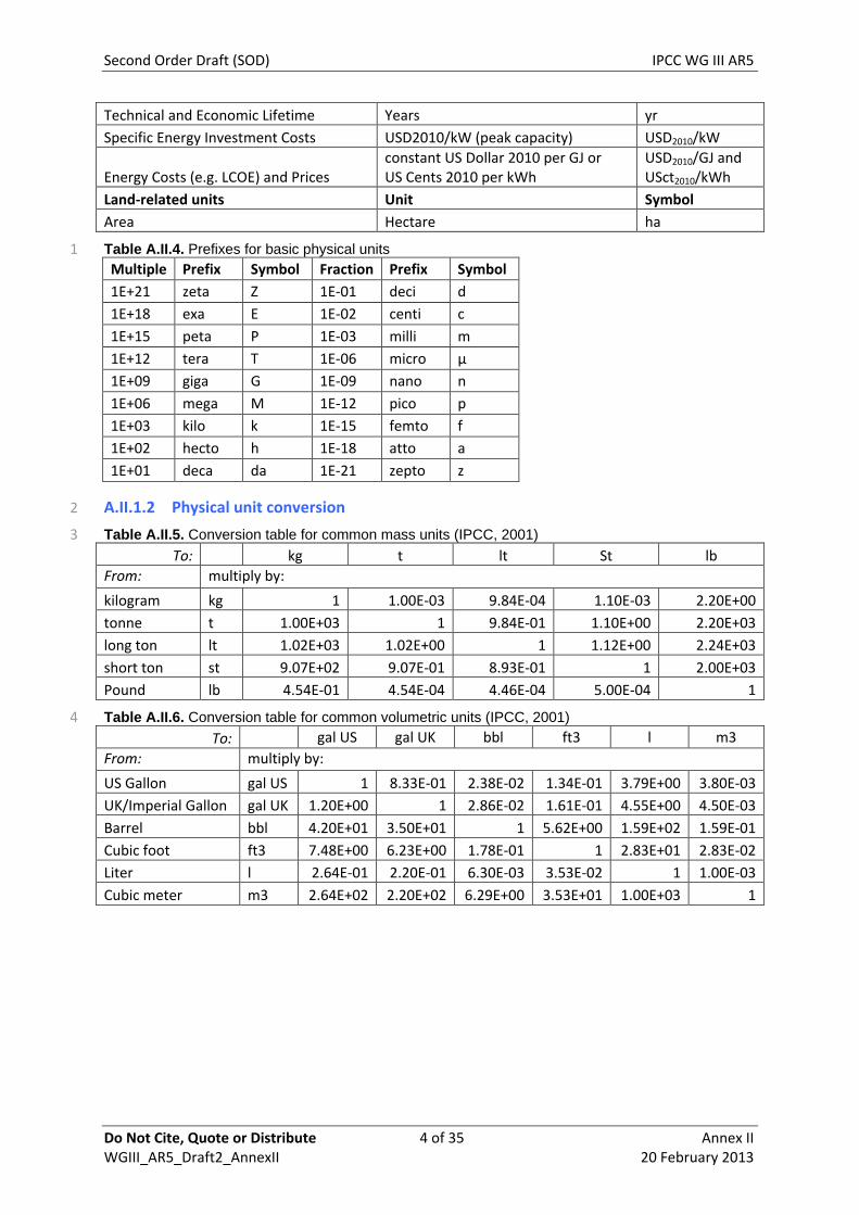
Technical and Economic Lifetime Years yr

Specific Energy Investment Costs USD2010/kW (peak capacity) USD2010/kW

Energy Costs (e.g. LCOE) and Prices constant US Dollar 2010 per GJ or US Cents 2010 per kWh

USD2010/GJ and USct2010/kWh

Land-related units Unit Symbol

Area Hectare ha

Table A.II.4. Prefixes for basic physical units 1

Multiple Prefix Symbol Fraction Prefix Symbol

1E+21 zeta Z 1E-01 deci d

1E+18 exa E 1E-02 centi c

1E+15 peta P 1E-03 milli m

1E+12 tera T 1E-06 micro μ

1E+09 giga G 1E-09 nano n

1E+06 mega M 1E-12 pico p

1E+03 kilo k 1E-15 femto f

1E+02 hecto h 1E-18 atto a

1E+01 deca da 1E-21 zepto z

A.II.1.2 Physical unit conversion 2

Table A.II.5. Conversion table for common mass units (IPCC, 2001) 3

To: kg t lt St lb

From: multiply by:

kilogram kg 1 1.00E-03 9.84E-04 1.10E-03 2.20E+00

tonne t 1.00E+03 1 9.84E-01 1.10E+00 2.20E+03

long ton lt 1.02E+03 1.02E+00 1 1.12E+00 2.24E+03

short ton st 9.07E+02 9.07E-01 8.93E-01 1 2.00E+03

Pound lb 4.54E-01 4.54E-04 4.46E-04 5.00E-04 1

Table A.II.6. Conversion table for common volumetric units (IPCC, 2001) 4

To: gal US gal UK bbl ft3 l m3

From: multiply by:

US Gallon gal US 1 8.33E-01 2.38E-02 1.34E-01 3.79E+00 3.80E-03

UK/Imperial Gallon gal UK 1.20E+00 1 2.86E-02 1.61E-01 4.55E+00 4.50E-03

Barrel bbl 4.20E+01 3.50E+01 1 5.62E+00 1.59E+02 1.59E-01

Cubic foot ft3 7.48E+00 6.23E+00 1.78E-01 1 2.83E+01 2.83E-02

Liter l 2.64E-01 2.20E-01 6.30E-03 3.53E-02 1 1.00E-03

Cubic meter m3 2.64E+02 2.20E+02 6.29E+00 3.53E+01 1.00E+03 1



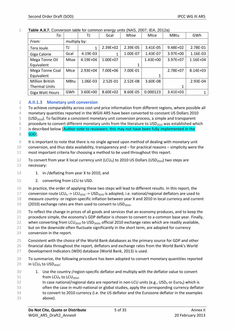
Table A.II.7. Conversion table for common energy units (NAS, 2007; IEA, 2012a) 1 To: TJ Gcal Mtoe Mtce MBtu GWh

From: multiply by:

Tera Joule TJ 1 2.39E+02 2.39E-05 3.41E-05 9.48E+02 2.78E-01

Giga Calorie Gcal 4.19E-03 1 1.00E-07 1.43E-07 3.97E+00 1.16E-03

Mega Tonne Oil Equivalent

Mtoe 4.19E+04 1.00E+07 1

1.43E+00 3.97E+07 1.16E+04

Mega Tonne Coal Equivalent

Mtce 2.93E+04 7.00E+06 7.00E-01 1

2.78E+07 8.14E+03

Million British Thermal Units

MBtu 1.06E-03 2.52E-01 2.52E-08 3.60E-08 1

2.93E-04

Giga Watt Hours GWh 3.60E+00 8.60E+02 8.60E-05 0.000123 3.41E+03 1

A.II.1.3 Monetary unit conversion 2

To achieve comparability across cost und price information from different regions, where possible all 3 monetary quantities reported in the WGIII AR5 have been converted to constant US Dollars 2010 4 (USD2010). To facilitate a consistent monetary unit conversion process, a simple and transparent 5 procedure to convert different monetary units from the literature to USD2010 was established which 6 is described below [Author note to reviewers: this may not have been fully implemented in the 7 SOD]. 8

It is important to note that there is no single agreed upon method of dealing with monetary unit 9 conversion, and thus data availability, transparency and – for practical reasons – simplicity were the 10 most important criteria for choosing a method to be used throughout this report. 11

To convert from year X local currency unit (LCUX) to 2010 US Dollars (USD2010) two steps are 12 necessary: 13

1. in-/deflating from year X to 2010, and 14

2. converting from LCU to USD. 15

In practice, the order of applying these two steps will lead to different results. In this report, the 16 conversion route LCUX -> LCU2010 -> USD2010 is adopted, i.e. national/regional deflators are used to 17 measure country- or region-specific inflation between year X and 2010 in local currency and current 18 (2010) exchange rates are then used to convert to USD2010. 19

To reflect the change in prices of all goods and services that an economy produces, and to keep the 20 procedure simple, the economy's GDP deflator is chosen to convert to a common base year. Finally, 21 when converting from LCU2010 to USD2010, official 2010 exchange rates which are readily available, 22 but on the downside often fluctuate significantly in the short term, are adopted for currency 23 conversion in the report. 24

Consistent with the choice of the World Bank databases as the primary source for GDP and other 25 financial data throughout the report, deflators and exchange rates from the World Bank’s World 26 Development Indicators (WDI) database (World Bank, 2013) is used. 27

To summarize, the following procedure has been adopted to convert monetary quantities reported 28 in LCUX to USD2010: 29

1. Use the country-/region-specific deflator and multiply with the deflator value to convert 30 from LCUX to LCU2010. 31 In case national/regional data are reported in non-LCU units (e.g., USDX or EuroX) which is 32 often the case in multi-national or global studies, apply the corresponding currency deflator 33 to convert to 2010 currency (i.e. the US deflator and the Eurozone deflator in the examples 34 above). 35



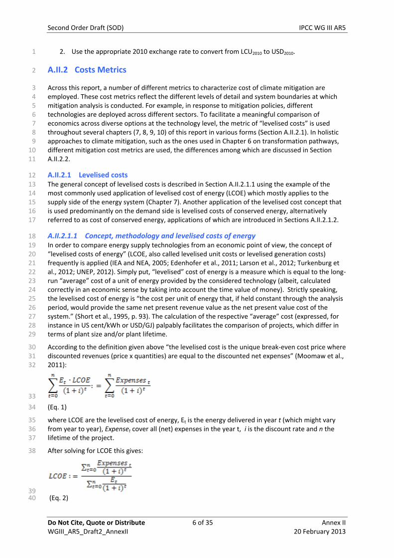
2. Use the appropriate 2010 exchange rate to convert from LCU2010 to USD2010. 1

A.II.2 Costs Metrics 2

Across this report, a number of different metrics to characterize cost of climate mitigation are 3 employed. These cost metrics reflect the different levels of detail and system boundaries at which 4 mitigation analysis is conducted. For example, in response to mitigation policies, different 5 technologies are deployed across different sectors. To facilitate a meaningful comparison of 6 economics across diverse options at the technology level, the metric of “levelised costs” is used 7 throughout several chapters (7, 8, 9, 10) of this report in various forms (Section A.II.2.1). In holistic 8 approaches to climate mitigation, such as the ones used in Chapter 6 on transformation pathways, 9 different mitigation cost metrics are used, the differences among which are discussed in Section 10 A.II.2.2. 11

A.II.2.1 Levelised costs 12

The general concept of levelised costs is described in Section A.II.2.1.1 using the example of the 13 most commonly used application of levelised cost of energy (LCOE) which mostly applies to the 14 supply side of the energy system (Chapter 7). Another application of the levelised cost concept that 15 is used predominantly on the demand side is levelised costs of conserved energy, alternatively 16 referred to as cost of conserved energy, applications of which are introduced in Sections A.II.2.1.2. 17

A.II.2.1.1 Concept, methodology and levelised costs of energy 18 In order to compare energy supply technologies from an economic point of view, the concept of 19 “levelised costs of energy” (LCOE, also called levelised unit costs or levelised generation costs) 20 frequently is applied (IEA and NEA, 2005; Edenhofer et al., 2011; Larson et al., 2012; Turkenburg et 21 al., 2012; UNEP, 2012). Simply put, “levelised” cost of energy is a measure which is equal to the long-22 run “average” cost of a unit of energy provided by the considered technology (albeit, calculated 23 correctly in an economic sense by taking into account the time value of money). Strictly speaking, 24 the levelised cost of energy is “the cost per unit of energy that, if held constant through the analysis 25 period, would provide the same net present revenue value as the net present value cost of the 26 system.” (Short et al., 1995, p. 93). The calculation of the respective “average” cost (expressed, for 27 instance in US cent/kWh or USD/GJ) palpably facilitates the comparison of projects, which differ in 28 terms of plant size and/or plant lifetime. 29

According to the definition given above “the levelised cost is the unique break-even cost price where 30 discounted revenues (price x quantities) are equal to the discounted net expenses” (Moomaw et al., 31 2011): 32

33

(Eq. 1) 34

where LCOE are the levelised cost of energy, Et is the energy delivered in year t (which might vary 35 from year to year), Expenset cover all (net) expenses in the year t, i is the discount rate and n the 36 lifetime of the project. 37

After solving for LCOE this gives: 38

39 (Eq. 2) 40



Note that while it appears as if energy amounts were discounted in Eq. 2, this is just an arithmetic 1 result of rearranging Eq. (1) (Branker et al., 2011). In fact, originally, revenues are discounted and not 2 energy amounts per se (see Eq. 1). 3

Considering energy conversion technologies, the lifetime expenses comprise investment costs I, 4 operation and maintenance cost O&M (including waste management costs), fuel costs F, carbon 5 costs C, and decommissioning costs D. In this case, levelised cost can be determined by (IEA and 6 NEA, 2005, p. 34): 7

8

(Eq. 3) 9

In simply cases, where the provided energy is constant during the lifetime of the project, this 10 translates to: 11

12 (Eq. 4) 13

where is the capital recovery factor and NPV the net present value of all lifetime 14

expenditures (Suerkemper et al., 2012). 15

The LCOE of a technology is not the sole determinant of its value or economic competitiveness. In 16 addition, integration and transmission costs, relative environmental impacts must be considered 17 (e.g., by using external costs), as well as the contribution of a technology to meeting specific energy 18 services, for example, peak electricity demands (Heptonstall, 2007). Joskow (2011) for instance, 19 pointed out that LCOE comparisons of intermittent generating technologies (such as solar energy 20 converters and wind turbines) with dispatchable power plants (e.g., coal or gas power plants) may 21 be misleading as theses comparisons fail to take into account the different production schedule and 22 the associated differences in the market value of the electricity that is provided. 23

Taking these shortcomings into account, there seems to be a clear understanding that LCOE are not 24 intended to be a definitive guide to actual electricity generation investment decisions e.g. (IEA and 25 NEA, 2005; DTI, 2006). Some studies suggest that the role of levelised costs is to give a ‘first order 26 assessment’ (EERE, 2004) of project viability. In order to capture the existing uncertainty, sensitivity 27 analyses, which are sometimes based on Monte Carlo methods, are frequently carried out in 28 numerical studies. Darling et al. (2011), for instance, suggest that transparency could be improved by 29 calculating LCOE as a distribution, constructed using input parameter distributions, rather than a 30 single number. Studies based on empirical data, in contrast, may suffer from using samples that do 31 not cover all cases. Summarizing country studies in an effort to provide a global assessment, for 32 instance, might have a bias as data for developing countries often are not available (IEA, 2012b). 33

As Section 7.8.2 shows, typical LCOE ranges are broad as values vary across the globe depending on 34 the site-specific renewable energy resource base, on local fuel and feedstock prices as well as on 35 country specific projected costs of investment, financing, and operation and maintenance. While 36 noting that system and installation costs vary widely, Branker et al. (2011) document significant 37 variations in the underlying assumptions that go into calculating LCOE for PV, with many analysts not 38 taking into account recent cost reductions or the associated technological advancements. In 39 summary, a comparison between different technologies should not be based on LCOE data solely; 40 instead, site-, project- and investor specific conditions should be considered. 41



A.II.2.1.2 Levelised costs of conserved energy 1

The concept of “levelised costs of conserved energy” (LCCE), or more frequently referred to as "cost 2 of conserved energy (CCE)", is very similar to the LCOE concept, primarily intended to be used for 3 comparing the cost of a unit of energy saved to the price/cost of providing energy. In essence the 4 concept, similarly to LCOE, also annualises the investment and operation and maintenance cost 5 differences between a baseline technology and the energy-efficiency alternative, and divides this 6 quantity by the annual energy savings (Brown et al., 2008). Similarly to LCOE, it also bridges the time 7 lag between the initial additional investment and the future energy savings through the application 8 of the capital recovery factor (Meier, 1983). Its conceptual formula is essentially the same as Eq. 4 9 above, with "E" meaning in this context the amount of energy saved annually (Hansen, 2012): 10

tE

ICRFCCE 11

(Eq. 5) 12

Where ΔI is the difference in investment costs of an energy saving measure (e.g. in USD) as 13 compared to a baseline investment; ΔEt is the annual energy conserved by the measure (e.g. in kWh) 14 as compared to the usage of the baseline technology; and CRF is the capital recovery factor 15 depending on the discount rate i and the lifetime of the measure n in years as defined above. 16

The key difference in the concept with LCOE is the usage of a reference/baseline technology. LCCE 17 can only be interpreted in context of a reference, and is thus very sensitive to how this reference is 18 chosen. For instance, the replacement of a very inefficient refrigerator can be very cost-effective, 19 but if we consider an already relatively efficient product as the reference technology, the CCE value 20 can be many times higher. 21

The main strength of the CCE concept is that it provides a metric of energy saving investments that 22 are independent of the energy price, and can thus be compared to different energy cost/price values 23 for determining the profitability of the investment. 24

For the calculation of CCE, a few challenges should be pinpointed. First of all, the lifetimes of the 25 efficient and the reference technology may be different. In this case the investment cost difference 26 needs to be used that incurs throughout the lifetime of the longer-living technology. For instance, a 27 compact fluorescent lamp (CFL) lasts as much as 10 times as long as an incandescent lamp, and thus 28 in the calculation of the CCE for a CFL replacing an incandescent lamp the cost difference of the CFL 29 and 10 incandescent lamps need to be used (Ürge-Vorsatz, 1996). In such a case, as in some other 30 cases, too, the difference can be negative, leading the CCE values to be negative. Negative CCE 31 values mean that the investment is already profitable at the investment level, without the need for 32 the energy savings to recover the extra investment costs. 33

In case there are operation and maintenance costs (OM) differences between the baseline and 34 efficient technology, these also enter the CCE calculation, similarly to Eq. 3 above: 35

tE

OMICRFCCE 36

(Eq. 6) 37

These can be important for applications where there are significant OM costs, for instance, the lamp 38 replacement on streetlamps, bridges. In such cases a longer-lifetime product, as it typically applies 39 to efficient lighting technologies, is already associated with negative costs at the investment level 40 (less frequent needs for labour to replace the lamps), and thus can result in significantly negative 41 CCEs or cost savings (Ürge-Vorsatz, 1996). 42



A.II.2.2 Mitigation cost metrics 1

There is no single metric for reporting the costs of mitigation, and the metrics that are available are 2 not directly comparable (see Section 3.10.2 for a more general discussion; see Section 6.3.6 for an 3 overview of costs used in model analysis). In economic theory the most direct cost measure is a 4 change in welfare due to changes in the amount and composition of consumption of goods and 5 services by individuals. Important measures of welfare change include “equivalent variation” and 6 “compensating variation” which attempt to discern how much individual income would need to 7 change to keep consumers just as well off after the imposition of a policy as before. However, these 8 are quite difficult to calculate, so a more common welfare measurement is change in consumption, 9 which captures the total amount of money consumers are able to spend on goods and services. 10 Another common metric is the change in gross domestic product (GDP). However, GDP is a less 11 satisfactory indicator of overall cost than those focused on individual income and consumption, 12 because it is a measure of output, which includes not only consumption, but also investment, 13 imports and exports, and government spending. A final common measure is the “deadweight loss” 14 or “area on the marginal abatement cost function”, which suffers from similar limitations as GDP. 15

From a practical perspective, different modelling frameworks applied in climate mitigation analysis 16 are capable of producing different cost estimates (Section 6.2). Therefore, when comparing cost 17 estimates across climate mitigation scenarios from different models, some degree of incomparability 18 must necessarily result. In representing costs across transformation pathways in this report and 19 more specifically Chapter 6, consumption losses are used preferentially when available from general 20 equilibrium models, and costs represented by the area under the marginal abatement cost function 21 or additional energy system costs are used for partial equilibrium measures. 22

One popular measure used in different studies to evaluate the economic implications of mitigation 23 actions is the emissions price, often presented in per metric ton of CO2 or, in case of multiple gases, 24 per metric ton of CO2-equivalent. However, it is important to emphasize that emissions prices are 25 not cost measures. There are two important reasons why emissions prices are not a meaningful 26 representation of costs. First, emissions prices measure marginal cost; that is, the cost of an 27 additional unit of emissions reduction. In contrast, total costs represent the costs of all mitigation 28 that took place at lower cost than the emissions price. Without explicitly accounting for these 29 “inframarginal” costs, it is impossible to know how the carbon price relates to total mitigation costs. 30 Second, emissions prices can interact with other policies and measures, either regulatory policies 31 directed at greenhouse gas reduction (for example, renewable portfolio standards or subsidies to 32 carbon-free technologies) or other taxes on energy, labour, or capital. If mitigation is achieved partly 33 by these other measures, the emissions price will not take into account the full costs of an additional 34 unit of emissions reductions, and will indicate a lower marginal cost than is actually warranted. 35

It is often important to calculate the total cost of mitigation borne over the life of the policy. To 36 compare costs over time, conventional economic practices apply a discount rate to future costs on 37 the basis that money today would earn a return over time. The discount rate, which represents how 38 much less society values the future payments in comparison to the present payments of the same 39 size, is a key parameter, and there are different views on what the appropriate rate is for climate 40 policy (see Section 3.6, (Portney and Weyant, 1999; Nordhaus, 2006; Stern, 2007)). Transformation 41 pathways in the literature have been derived under a range of assumptions about discount rates. 42

A.II.3 Primary energy accounting 43

Following the standard set by the IPCC Special Report on Renewable Energy Sources and Climate 44 Change Mitigation (SRREN), this report adopts the direct-equivalent accounting method for the 45 reporting of primary energy from non-combustible energy sources. The following section largely 46 draws from Annex II of the SRREN (Moomaw et al., 2011) and summarizes the most relevant points. 47



Different energy analyses use a variety of accounting methods that lead to different quantitative 1 outcomes for both reporting of current primary energy use and energy use in scenarios that explore 2 future energy transitions. Multiple definitions, methodologies and metrics are applied. Energy 3 accounting systems are utilized in the literature often without a clear statement as to which system 4 is being used (Lightfoot, 2007; Martinot et al., 2007). An overview of differences in primary energy 5 accounting from different statistics has been described by Macknick (2011) and the implications of 6 applying different accounting systems in long-term scenario analysis were illustrated by Nakicenovic 7 et al., (1998), Moomaw et al. (2011) and Grubler et al. (2012). 8

Three alternative methods are predominantly used to report primary energy. While the accounting 9 of combustible sources, including all fossil energy forms and biomass, is identical across the different 10 methods, they feature different conventions on how to calculate primary energy supplied by non-11 combustible energy sources, i.e. nuclear energy and all renewable energy sources except biomass. 12 These methods are: 13

the physical energy content method adopted, for example, by the OECD, the International 14 Energy Agency (IEA) and Eurostat (IEA/OECD/Eurostat, 2005), 15

the substitution method which is used in slightly different variants by BP (2012) and the US 16 Energy Information Administration (EIA, 2012a, b, Table A6), both of which publish 17 international energy statistics, and 18

the direct equivalent method that is used by UN Statistics (2010) and in multiple IPCC reports 19 that deal with long-term energy and emission scenarios (Nakicenovic and Swart, 2000; 20 Morita et al., 2001; Fisher et al., 2007; Fischedick et al., 2011). 21

For non-combustible energy sources, the physical energy content method adopts the principle that 22 the primary energy form should be the first energy form used down-stream in the production 23 process for which multiple energy uses are practical (IEA/OECD/Eurostat, 2005). This leads to the 24 choice of the following primary energy forms: 25

heat for nuclear, geothermal and solar thermal, and 26

electricity for hydro, wind, tide/wave/ocean and solar PV. 27

Using this method, the primary energy equivalent of hydro energy and solar PV, for example, 28 assumes a 100% conversion efficiency to “primary electricity”, so that the gross energy input for the 29 source is 3.6 MJ of primary energy = 1 kWh electricity. Nuclear energy is calculated from the gross 30 generation by assuming a 33% thermal conversion efficiency1, i.e. 1 kWh = (3.6 ÷ 0.33) = 10.9 MJ. For 31 geothermal, if no country-specific information is available, the primary energy equivalent is 32 calculated using 10% conversion efficiency for geothermal electricity (so 1 kWh = (3.6 ÷ 0.1) = 36 33 MJ), and 50% for geothermal heat. 34

The substitution method reports primary energy from non-combustible sources in such a way as if 35 they had been substituted for combustible energy. Note, however, that different variants of the 36 substitution method use somewhat different conversion factors. For example, BP applies 38% 37 conversion efficiency to electricity generated from nuclear and hydro whereas the World Energy 38 Council used 38.6% for nuclear and non-combustible renewables (WEC, 1993; Grübler et al., 1996; 39 Nakicenovic et al., 1998), and EIA uses still different values. For useful heat generated from non-40 combustible energy sources, other conversion efficiencies are used. Macknick (2011) provides a 41 more complete overview. 42

1 As the amount of heat produced in nuclear reactors is not always known, the IEA estimates the primary energy equivalent from the electricity generation by assuming an efficiency of 33%, which is the average of nuclear power plants in Europe (IEA, 2012b).



The direct equivalent method counts one unit of secondary energy provided from non-combustible 1 sources as one unit of primary energy, i.e. 1 kWh of electricity or heat is accounted for as 1 kWh = 2 3.6 MJ of primary energy. This method is mostly used in the long-term scenarios literature, including 3 multiple IPCC reports (Watson et al., 1995; Nakicenovic and Swart, 2000; Morita et al., 2001; Fisher 4 et al., 2007; Fischedick et al., 2011), because it deals with fundamental transitions of energy systems 5 that rely to a large extent on low-carbon, non-combustible energy sources. 6

The accounting of combustible sources, including all fossil energy forms and biomass, includes some 7 ambiguities related to the definition of the heating value of combustible fuels. The higher heating 8 value (HHV), also known as gross calorific value (GCV) or higher calorific value (HCV), includes the 9 latent heat of vaporisation of the water produced during combustion of the fuel. In contrast, the 10 lower heating value (LHV) (also: net calorific value (NCV) or lower calorific value (LCV)) excludes this 11 latent heat of vaporization. For coal and oil, the LHV is about 5% less than the HHV, for most forms 12 of natural and manufactured gas the difference is 9-10%, while for electricity and heat there is no 13 difference as the concept has no meaning in this case (IEA, 2012a). 14

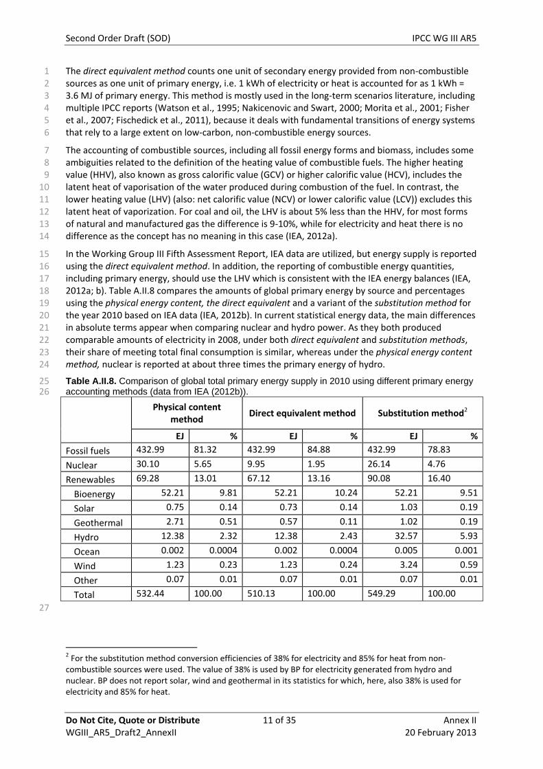
In the Working Group III Fifth Assessment Report, IEA data are utilized, but energy supply is reported 15 using the direct equivalent method. In addition, the reporting of combustible energy quantities, 16 including primary energy, should use the LHV which is consistent with the IEA energy balances (IEA, 17 2012a; b). Table A.II.8 compares the amounts of global primary energy by source and percentages 18 using the physical energy content, the direct equivalent and a variant of the substitution method for 19 the year 2010 based on IEA data (IEA, 2012b). In current statistical energy data, the main differences 20 in absolute terms appear when comparing nuclear and hydro power. As they both produced 21 comparable amounts of electricity in 2008, under both direct equivalent and substitution methods, 22 their share of meeting total final consumption is similar, whereas under the physical energy content 23 method, nuclear is reported at about three times the primary energy of hydro. 24

Table A.II.8. Comparison of global total primary energy supply in 2010 using different primary energy 25 accounting methods (data from IEA (2012b)). 26

Physical content method

Direct equivalent method Substitution method2

EJ % EJ % EJ %

Fossil fuels 432.99 81.32 432.99 84.88 432.99 78.83

Nuclear 30.10 5.65 9.95 1.95 26.14 4.76

Renewables 69.28 13.01 67.12 13.16 90.08 16.40

Bioenergy 52.21 9.81 52.21 10.24 52.21 9.51

Solar 0.75 0.14 0.73 0.14 1.03 0.19

Geothermal 2.71 0.51 0.57 0.11 1.02 0.19

Hydro 12.38 2.32 12.38 2.43 32.57 5.93

Ocean 0.002 0.0004 0.002 0.0004 0.005 0.001

Wind 1.23 0.23 1.23 0.24 3.24 0.59

Other 0.07 0.01 0.07 0.01 0.07 0.01

Total 532.44 100.00 510.13 100.00 549.29 100.00

27

2 For the substitution method conversion efficiencies of 38% for electricity and 85% for heat from non-combustible sources were used. The value of 38% is used by BP for electricity generated from hydro and nuclear. BP does not report solar, wind and geothermal in its statistics for which, here, also 38% is used for electricity and 85% for heat.



The alternative methods outlined above emphasize different aspects of primary energy supply. 1 Therefore, depending on the application, one method may be more appropriate than another. 2 However, none of them is superior to the others in all facets. In addition, it is important to realize 3 that total primary energy supply does not fully describe an energy system, but is merely one 4 indicator amongst many. Energy balances as published by IEA (2012a; b) offer a much wider set of 5 indicators which allows tracing the flow of energy from the resource to final energy use. For 6 instance, complementing total primary energy consumption by other indicators, such as total final 7 energy consumption (TFC) and secondary energy production (e.g., electricity, heat), using different 8 sources helps link the conversion processes with the final use of energy. 9

A.II.4 Carbon footprinting, lifecycle assessment, material flow analysis 10

In AR5, findings from carbon footprinting, life cycle assessment and material flow analysis are used 11 in Chapters 4, 5, 7, 8, 9, 11, and 12. The following section briefly sketches the intellectual 12 background of these methods and discusses their usefulness for climate mitigation research, and 13 some relevant assumptions, limitations and methodological discussions. 14

The anthropogenic contributions to climate change, caused by fossil fuel combustion, land 15 conversion for agriculture, commercial forestry and infrastructure, and numerous agricultural and 16 industrial processes, result from the use of natural resources, i.e. the manipulation of material and 17 energy flows by humans for human purposes. Climate mitigation research has a long tradition of 18 addressing the energy flows and associated emissions, however, the sectors involved in energy 19 supply and use are coupled with each other through material stocks and flows, which leads to 20 feedbacks and delays. These linkages between energy and material stocks and flows have, despite 21 their considerable relevance for GHG emissions, so far gained little attention in climate change 22 mitigation (and adaptation). The research agendas of industrial ecology and ecological economics 23 with their focus on the socioeconomic metabolism (Wolman, 1965; Baccini and Brunner, 1991; Ayres 24 and Simonis, 1994; Fischer-Kowalski and Haberl, 1997) a.k.a. biophysical economy (Cleveland et al., 25 1984), can complement energy assessments in important manners and support the development of 26 a broader framing of climate mitigation research as part of sustainability science. Socioeconomic 27 metabolism consists of the physical stocks and flows with which a society maintains and reproduces 28 itself (Fischer-Kowalski and Haberl, 2007). These research traditions are relevant for sustainability 29 because they comprehensively account for resource flows and hence allow to address the dynamics, 30 efficiency and emissions of production systems that convert or utilize resources to provide goods 31 and services to final consumers. Central to the socio-metabolic research methods are material and 32 energy balance principles applied at various scales ranging from individual production processes to 33 companies, regions, value chains, economic sectors, and nations. 34

A.II.4.1 Material flow analysis 35

Material flow analysis (MFA) – including substance flow analysis (SFA) – is a method for describing, 36 modeling (using socio-economic and technological drivers), simulating (scenario development), and 37 visualizing the socioeconomic stocks and flows of matter and energy in systems defined in space and 38 time to inform policies on resource and waste management and pollution control. Mass- and energy 39 balance consistency is enforced at the level of goods and/or individual substances. As a result of the 40 application of consistency criteria they are useful to analyze feedbacks within complex systems, e.g. 41 the interrelations between diets, food production in cropland and livestock systems, and availability 42 of area for bioenergy production (e.g., (Erb et al., 2012), see chapter 11, section 11.4). 43

The concept of socioeconomic metabolism (Ayres and Kneese, 1969; Boulding, 1972; Martinez-Alier, 44 1987; Baccini and Brunner, 1991; Ayres and Simonis, 1994; Fischer-Kowalski and Haberl, 1997) has 45 been developed as an approach to study the extraction of materials or energy from the 46 environment, their conversion in production and consumption processes, and the resulting outputs 47 to the environment. Accordingly, the unit of analysis is the socioeconomic system (or some of its 48



components), treated as a systemic entity, in analogy to an organism or a sophisticated machine that 1 requires material and energy inputs from the natural environment in order to carry out certain 2 defined functions and that results in outputs such as wastes and emissions. 3

Some MFAs trace the stocks and flows of aggregated groups of materials (fossil fuels, biomass, ores 4 and industrial minerals, construction materials) through societies and can be performed on the 5 global scale (Krausmann et al., 2009), for national economies and groups of countries (Weisz et al., 6 2006), urban systems (Wolman, 1965) or other socioeconomic subsystems. Similarly comprehensive 7 methods that apply the same system boundaries have been developed to account for energy flows 8 (Haberl, 2001a), (Haberl, 2001b), (Haberl et al., 2006), carbon flows (Erb et al., 2008) and biomass 9 flows (Krausmann et al., 2008) and are often subsumed in the Material and Energy Flow Accounting 10 (MEFA) framework (Haberl et al., 2004). Other MFAs have been conducted for analyzing the cycles of 11 individual substances (e.g., carbon, nitrogen, or phosphorus cycles (Erb et al., 2008)) or metals (e.g., 12 copper, iron, or cadmium cycles; (Graedel and Cao, 2010)) within socio-economic systems. A third 13 group of MFAs have a focus on individual processes with an aim to balance a wide variety of goods 14 and substances (e.g., waste incineration, a shredder plant, or a city). 15

The MFA approach has also been extended towards the analysis of socio-ecological systems, i.e. 16 coupled human-environment systems. One example for this research strand is the ‘human 17 appropriation of net primary production’ or HANPP which assesses human-induced changes in 18 biomass flows in terrestrial ecosystems (Vitousek et al., 1986)(Wright, 1990)(Imhoff et al., 19 2004)(Haberl et al., 2007). The socio-ecological metabolism approach is particularly useful for 20 assessing feedbacks in the global land system, e.g. interrelations between production and 21 consumption of food, agricultural intensity, livestock feeding efficiency and bioenergy potentials, 22 both residue potentials and area availability for energy crops (Erb et al., 2012)(Haberl et al., 2011). 23

Anthropogenic stocks (built environment) play a crucial role in socio-metabolic systems: (i) they 24 provide services to the inhabitants, (ii) their operation often requires energy and releases emissions, 25 (iii) increase or renewal/maintenance of these stocks requires materials, and (iv) the stocks embody 26 materials (often accumulated over the past decades or centuries) that may be recovered at the end 27 of the stocks’ service lives (“urban mining”) and, when recycled or reused, substitute primary 28 resources and save energy and emissions in materials production (Müller et al., 2006). In contrast to 29 flow variables, which tend to fluctuate much more, stock variables usually behave more robustly and 30 are therefore often suitable as drivers for developing long-term scenarios (Müller, 2006). The 31 exploration of built environment stocks (secondary resources), including their composition, 32 performance, and dynamics, is therefore a crucial pre-requisite for examining long-term 33 transformation pathways (Liu et al., 2012). Anthropogenic stocks have therefore been described as 34 the engines of socio-metabolic systems. Moreover, socioeconomic stocks sequester carbon (Lauk et 35 al., 2012); hence policies to increase the C content of long-lived infrastructures may contribute to 36 climate-change mitigation (Gustavsson et al., 2006). 37

So far, MFAs have been used mainly to inform policies for resource and waste management. Studies 38 with an explicit focus on climate change mitigation are less frequent, but rapidly growing. Examples 39 involve the exploration of long-term mitigation pathways for the iron/steel industry (Pauliuk et al 40 2012, Milford et al 2012), the aluminium industry (Liu et al., 2011)(Liu et al., 2012), the vehicle stock 41 (Melaina and Webster, 2011), (Pauliuk et al., 2011) or the building stock (Pauliuk et al., 2012). 42

A.II.4.2 Carbon footprinting and input-output analysis 43

Input-output analysis is an approach to trace the production process of products by economic 44 sectors, and their use as intermediate demand by producing sectors (industries) and final demand 45 including that by households and the public sector (Miller and Blair, 1985). Input-output tables 46 describe the structure of the economy, i.e. the interdependence of different producing sectors and 47 their role in final demand. Input-output tables are produced as part of national economic accounts 48 (Leontief, 1936). Through the assumption of fixed input coefficients, input-output models can be 49



formed, determining, e.g., the economic activity in all sectors required to produce a unit of final 1 demand. The mathematics of input-output analysis can be used with flows denoted in physical or 2 monetary units and has been applied also outside economics, e.g. to describe energy and nutrient 3 flows in ecosystems (Hannon et al., 1986). 4

Environmental applications of input-output analysis include analyzing the economic role of 5 abatement sectors (Leontief, 1971), quantifying embodied energy (Bullard and Herendeen, 1975) 6 and the employment benefits of energy efficiency measures (Hannon et al., 1978), describing the 7 benefits of pre-consumer scrap recycling (Nakamura and Kondo, 2001), tracing the material 8 composition of vehicles (Nakamura et al., 2007), and identifying the environmentally global division 9 of labor (Stromman et al., 2009). Important for climate mitigation research, input-output analysis 10 has been used to estimate the greenhouse gas emissions associated with the production and 11 delivery of goods for final consumption, the “carbon footprint” (Wiedmann and Minx, 2008). This 12 type of analysis basically redistributes the emissions occurring in producing sectors to final 13 consumption. It can be used to quantify GHG emissions associated with import and export (Wyckoff 14 and Roop, 1994), with national consumption (Hertwich and Peters, 2009), or the consumption of 15 specific groups of society (Lenzen and Schaeffer, 2004), regions (Turner et al., 2007) or institutions 16 (Berners-Lee et al., 2011)(Larsen and Hertwich, 2009)(Minx et al., 2009)(Peters, 2010).3 17

Global, multiregional input-output models are currently seen as the state-of-the-art tool to quantify 18 “consumer responsibility” (Ch.5)(Wiedmann et al., 2011)(Hertwich, 2011). Multiregional tables are 19 necessary to adequately represent national production patterns and technologies in the increasing 20 number of globally sourced products. Important insights provided to climate mitigation research is 21 the quantification of the total CO2 emissions embodied in global trade (Peters and Hertwich, 2008) 22 and the South->North directionality of trade (Peters, Minx, et al., 2011), to show that the UK 23 (Druckman et al., 2008)(Wiedmann et al., 2010) and other Annex B countries have increasing carbon 24 footprints while their territorial emissions are decreasing, to identify the contribution of different 25 commodity exports to the rapid growth in China’s greenhouse gas emissions (Xu et al., 2009), and to 26 quantify the income elasticity of the carbon footprint of different consumption categories like food, 27 mobility, and clothing (Hertwich and Peters, 2009). 28

Input-output models have an increasingly important instrumental role in climate mitigation. They 29 are used as a backbone for consumer carbon calculators, to provide sometimes spatially explicit 30 regional analysis (Lenzen et al., 2004), to help companies and public institutions target climate 31 mitigation efforts , and to provide initial estimates of emissions associated with different 32 alternatives (Minx et al., 2009). 33

Input-output calculations are usually based on industry-average production patterns and emissions 34 intensities and do not provide an insight into marginal emissions caused by additional purchases. 35 However, efforts to estimate future and marginal production patterns and emissions intensities exist 36 (Lan et al., 2012). At the same time, economic sector classifications in many countries are not very 37 fine, so that IO tables provide carbon footprint averages of broad product groups rather than specific 38 products. Many models use monetary units and are not good at addressing waste management and 39 recycling opportunities, although hybrid models with a physical representation of end-of-life 40 processes do exist (Nakamura and Kondo, 2001). At the time of publication, national input-output 41 tables describe the economy several years ago. Multiregional input-output tables are produced as 42 part of research efforts and need to reconcile different national conventions for the construction of 43 the tables and conflicting international trade data (Tukker et al., 2013). Efforts to provide a higher 44 level of detail of environmentally relevant sectors and to now-cast tables are currently under 45 development (Lenzen et al., 2012). 46

3 So far, only GHG emissions related to fossil fuel combustion and cement production are included in the „carbon footprint“; more data work is needed to address GHG emissions related to land-use change.



A.II.4.3 Life cycle assessment 1

Product life cycle assessment (LCA) was developed as a method to determine the embodied energy 2 use (Boustead and Hancock, 1979) and environmental pressures associated with specific product 3 systems (Finnveden et al., 2009). A product system describes the production, distribution, operation, 4 maintenance, and disposal of the product. From the beginning, the assessment of energy 5 technologies has been important, addressing questions such as how many years of use would be 6 required to recover the energy expended in producing a photovoltaic cell (Kato et al., 1998). 7 Applications in the consumer products industry addressing questions of whether cloth or paper 8 nappies (diapers) are more environmentally friendly (Vizcarra et al., 1994), or what type of washing 9 powder, prompted the development of a wider range of impact assessment methods addressing 10 issues such as aquatic toxicity (Gandhi et al., 2010), eutrophication and acidification (Huijbregts et 11 al., 2000). By now, a wide range of methods has been developed addressing either the contribution 12 to specific environmental problems (midpoint methods) or the damage caused to ecosystem or 13 human health (endpoint methods). At the same time, commonly used databases have collected life 14 cycle inventory information for materials, energy products, transportation services, chemicals and 15 other widely used products. Together, these methods form the backbone for the wide application of 16 LCA in industry and for environmental product declarations, as well as in policy. 17

LCA plays an increasingly important role in climate mitigation research (SRREN Annex II, Moomaw et 18 al. (2011)). In AR5, life cycle assessment has been used to quantify the greenhouse gas emissions 19 associated with technologies used for GHG mitigation, e.g., wind power, heat recovery ventilation 20 systems or carbon capture and storage. LCA is thus used to estimate the technical emissions 21 reductions offered by these technologies. 22

LCA has also been used to quantify co-benefits and detrimental side effects of mitigation 23 technologies and measures, including other environmental problems and the use of resources such 24 as water, land, and metals. LCA traditionally focuses only on GHG emissions, often evaluated over a 25 100 year time horizon. Radiation-based climate metrics (Peters, Aamaas, et al., 2011) and 26 geophysical effects such as albedo changes or indirect climate effects (Bright et al., 2012) have only 27 recently been addressed. 28

Life-cycle inventories are normally derived from empirical information on actual processes or 29 modeled based on engineering calculations. A key aspect of life cycle inventories for energy 30 technologies is that they contribute to understanding the thermodynamics of the wider product 31 system; combined with appropriate engineering insight, they can provide some upper bound for 32 possible technological improvements. These process LCAs provide detail and specificity, but do 33 usually not cover all input requirements as this would be too demanding. The cut-off error is the part 34 of the inventory that is not covered by conventional process analysis; it is commonly between 20-35 50% of the total impact (Lenzen, 2001). Hybrid life cycle assessment utilizes input-output models to 36 cover inputs of services or items that are used in small quantities (Treloar, 1996)(Suh et al., 37 2004)(Williams et al., 2009). Through their better coverage of the entire product system, hybrid LCAs 38 tend to more accurately represent all inputs to production (Majeau-Bettez et al., 2011). They have 39 also been used to estimate the cut-off error of process LCAs (Norris, 2002)(Deng et al., 2011). 40

It must be emphasized that LCA is a research method that answers specific research questions. To 41 understand how to interpret and use the results of an LCA case study, it is important to understand 42 what the research question is. The research questions “what are the environmental impacts of 43 product x” or “… of technology y” needs to be specified with respect to timing, regional context, 44 operational mode, background system etc. Modeling choices and assumption thus become part of 45 an LCA. This implies that LCA studies are not always comparable because they do not address the 46 same research question. Further, most LCAs are interpreted strictly on a functional unit basis; 47 expressing the impact of a unit of the product system in a described production system, without 48 either up-scaling the impacts to total impacts in the entire economy or saying something about the 49 scale-dependency of the activity. For example, an LCA may identify the use of recycled material as 50



beneficial, but the supply of recycled material is limited by the availability of suitable waste, so that 1 an up-scaling of recycling is not feasible. Hence, an LCA that shows that recycling is beneficial is not 2 sufficient to document the availability of further opportunities to reduce emissions. LCA, however, 3 coupled with an appropriate system models (using material flow data) is suitable to model the 4 emission gains from the expansion of further recycling activities. 5

LCA was developed with the intention to quantify resource use and emissions associated with 6 existing or prospective product systems, where the association reflects physical causality within 7 economic systems. Depending on the research question, it can be sensible to investigate average or 8 marginal inputs to production. Departing from this descriptive approach, it has been proposed to 9 model a wider socioeconomic causality describing the consequences of actions (Ekvall and Weidema, 10 2004). While established methods and a common practice exist for descriptive or “attributional” 11 LCA, such methods and standard practice are not yet established in “consequential” LCA (Zamagni et 12 al., 2012). Consequential LCAs are dependent on the decision context. It is increasingly 13 acknowledged in LCA that for investigating larger sustainability questions, the product focus is not 14 sufficient and larger system changes need to be modeled as such . 15

For climate mitigation analysis, it is useful to put LCA in a wider scenario context (Arvesen and 16 Hertwich, 2011; Viebahn et al., 2011). The purpose is to better understand the contribution a 17 technology can make to climate mitigation and to quantify the magnitude of its resource 18 requirements, co-benefits and side effects. For mitigation technologies on both the demand and 19 supply side, important contributors to the total impact are usually energy, materials and transport. 20 Understanding these contributions is already valuable for mitigation analysis. As all of these sectors 21 will change as part of the scenario, LCA-based scenarios show how much impacts per unit are likely 22 to change as part of the scenario. 23

Some LCAs take into account behavioral responses to different technologies (Takase et al., 2005; 24 Girod et al., 2011). Here, two issues must be distinguished. One is the use of the technology. For 25 example, it has been found that better insulated houses consistently are heated or cooled to 26 higher/lower average temperature (Haas and Schipper, 1998)(Greening et al., 2001). Not all of the 27 theoretically possible technical gain in energy efficiency results in reduced energy use (Sorrell and 28 Dimitropoulos, 2008). Such direct rebound effects can be taken into account through an appropriate 29 definition of the energy services compared, which do not necessarily need to be identical in terms of 30 the temperature or comfort levels. Another issue are larger market-related effects and spill-over 31 effects. A better insulated house leads to energy savings. Both questions of (1) whether the saved 32 energy would then be used elsewhere in the economy rather than not produced, and (2) what the 33 consumer does with the money saved, are not part of the product system and hence of product life 34 cycle assessment. They are sometimes taken up in LCA studies, quantified and compared. However, 35 for climate mitigation analysis, these mechanisms need to be addressed by scenario models on a 36 macro level. (See also section 11.4 for a discussion of such systemic effects). 37

A.II.5 Fat Tailed Distributions 38

If we have observed N independent loss events from a given loss distribution, the probability that 39 the next loss event will be worse than all the others is 1/(N+1). How much worse it will be depends 40 on the tail of the loss distribution. Many loss distributions including losses due to hurricanes are very 41 fat tailed. The notion of a "fat tailed distribution" may be given a precise mathematical meaning in 42 several ways, each capturing different intuitions. Older definitions refer to “fat tails” as “leptokurtic” 43 meaning that the tails are fatter than the normal distribution. Nowadays, mathematical definitions 44 are most commonly framed in terms of regular variation or subexponentiality (Embrechts et al., 45 1997). 46

A positive random variable X has regular variation with tail index α > 0 if the probability P(X > x) of 47

exceeding a value x decreases at a polynomial rate x- as x gets large. For any r > α, the r-th 48



moment of X is infinite, the α-th moment may be finite or infinite depending on the distribution. If 1 the first moment is infinite, then running averages of independent realizations of X increase to 2 infinity. If the second moment is infinite, then running averages have an infinite variance and do not 3 converge to a finite value. In either case, historical averages have little predictive value. The gamma, 4 exponential, and Weibull distributions all have finite r-th moment for all positive r. 5

A positive random variable X is subexponential if for any n independent copies X1,…Xn, the 6 probability that the sum X1+...+Xn exceeds a value x becomes identical to the probability that the 7 maximum of X1,…Xn exceeds x, as x gets large. In other words, ‘the sum of X1,…Xn is driven by the 8 largest of the X1,…Xn.' Every regularly varying distribution is subexponential, but the converse does 9 not hold. The Weibull distribution with shape parameter less than one is subexponential but not 10 regularly varying. All its moments are finite, but the sum of n independent realizations tends to be 11 dominated by the single largest value. 12

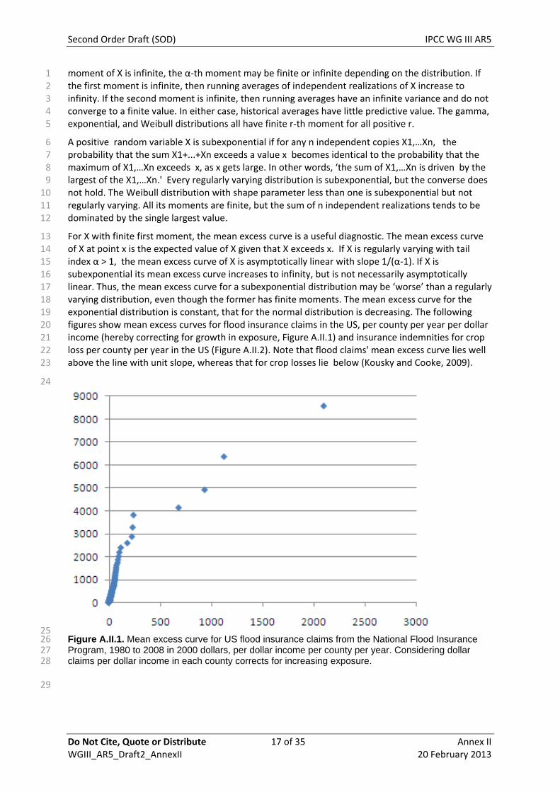
For X with finite first moment, the mean excess curve is a useful diagnostic. The mean excess curve 13 of X at point x is the expected value of X given that X exceeds x. If X is regularly varying with tail 14 index α > 1, the mean excess curve of X is asymptotically linear with slope 1/(α-1). If X is 15 subexponential its mean excess curve increases to infinity, but is not necessarily asymptotically 16 linear. Thus, the mean excess curve for a subexponential distribution may be ‘worse’ than a regularly 17 varying distribution, even though the former has finite moments. The mean excess curve for the 18 exponential distribution is constant, that for the normal distribution is decreasing. The following 19 figures show mean excess curves for flood insurance claims in the US, per county per year per dollar 20 income (hereby correcting for growth in exposure, Figure A.II.1) and insurance indemnities for crop 21 loss per county per year in the US (Figure A.II.2). Note that flood claims' mean excess curve lies well 22 above the line with unit slope, whereas that for crop losses lie below (Kousky and Cooke, 2009). 23

24

25 Figure A.II.1. Mean excess curve for US flood insurance claims from the National Flood Insurance 26 Program, 1980 to 2008 in 2000 dollars, per dollar income per county per year. Considering dollar 27 claims per dollar income in each county corrects for increasing exposure. 28

29



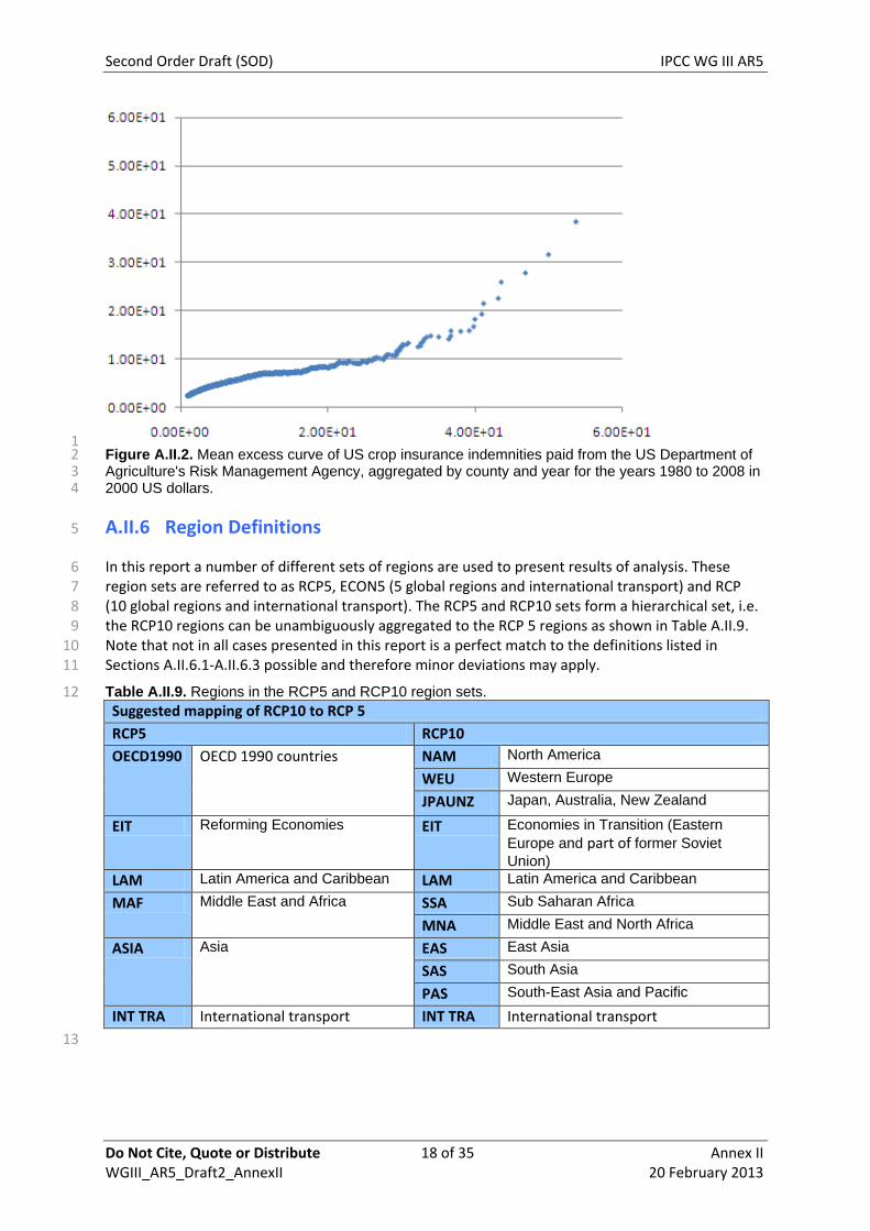
1 Figure A.II.2. Mean excess curve of US crop insurance indemnities paid from the US Department of 2 Agriculture's Risk Management Agency, aggregated by county and year for the years 1980 to 2008 in 3 2000 US dollars. 4

A.II.6 Region Definitions 5

In this report a number of different sets of regions are used to present results of analysis. These 6 region sets are referred to as RCP5, ECON5 (5 global regions and international transport) and RCP 7 (10 global regions and international transport). The RCP5 and RCP10 sets form a hierarchical set, i.e. 8 the RCP10 regions can be unambiguously aggregated to the RCP 5 regions as shown in Table A.II.9. 9 Note that not in all cases presented in this report is a perfect match to the definitions listed in 10 Sections A.II.6.1-A.II.6.3 possible and therefore minor deviations may apply. 11

Table A.II.9. Regions in the RCP5 and RCP10 region sets. 12 Suggested mapping of RCP10 to RCP 5

RCP5 RCP10

OECD1990 OECD 1990 countries NAM North America

WEU Western Europe

JPAUNZ Japan, Australia, New Zealand

EIT Reforming Economies EIT Economies in Transition (Eastern

Europe and part of former Soviet

Union)

LAM Latin America and Caribbean LAM Latin America and Caribbean

MAF Middle East and Africa SSA Sub Saharan Africa

MNA Middle East and North Africa

ASIA Asia EAS East Asia

SAS South Asia

PAS South-East Asia and Pacific

INT TRA International transport INT TRA International transport

13



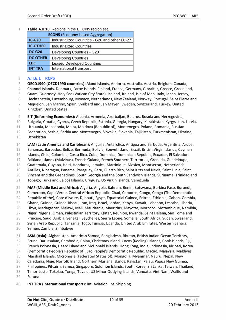
Table A.II.10. Regions in the ECON5 region set. 1

ECON5 (Economy-based Aggregation)

IC-G20 Industrialized Countries - G20 and other EU-27

IC-OTHER Industrialized Countries

DC-G20 Developing Countries - G20

DC-OTHER Developing Countries

LDC Leased Developed Countries

INT TRA International transport

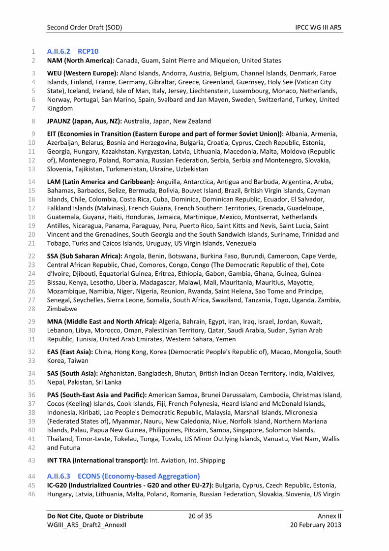
A.II.6.1 RCP5 2

OECD1990 (OECD1990 countries): Aland Islands, Andorra, Australia, Austria, Belgium, Canada, 3 Channel Islands, Denmark, Faroe Islands, Finland, France, Germany, Gibraltar, Greece, Greenland, 4 Guam, Guernsey, Holy See (Vatican City State), Iceland, Ireland, Isle of Man, Italy, Japan, Jersey, 5 Liechtenstein, Luxembourg, Monaco, Netherlands, New Zealand, Norway, Portugal, Saint Pierre and 6 Miquelon, San Marino, Spain, Svalbard and Jan Mayen, Sweden, Switzerland, Turkey, United 7 Kingdom, United States 8

EIT (Reforming Economies): Albania, Armenia, Azerbaijan, Belarus, Bosnia and Herzegovina, 9 Bulgaria, Croatia, Cyprus, Czech Republic, Estonia, Georgia, Hungary, Kazakhstan, Kyrgyzstan, Latvia, 10 Lithuania, Macedonia, Malta, Moldova (Republic of), Montenegro, Poland, Romania, Russian 11 Federation, Serbia, Serbia and Montenegro, Slovakia, Slovenia, Tajikistan, Turkmenistan, Ukraine, 12 Uzbekistan 13

LAM (Latin America and Caribbean): Anguilla, Antarctica, Antigua and Barbuda, Argentina, Aruba, 14 Bahamas, Barbados, Belize, Bermuda, Bolivia, Bouvet Island, Brazil, British Virgin Islands, Cayman 15 Islands, Chile, Colombia, Costa Rica, Cuba, Dominica, Dominican Republic, Ecuador, El Salvador, 16 Falkland Islands (Malvinas), French Guiana, French Southern Territories, Grenada, Guadeloupe, 17 Guatemala, Guyana, Haiti, Honduras, Jamaica, Martinique, Mexico, Montserrat, Netherlands 18 Antilles, Nicaragua, Panama, Paraguay, Peru, Puerto Rico, Saint Kitts and Nevis, Saint Lucia, Saint 19 Vincent and the Grenadines, South Georgia and the South Sandwich Islands, Suriname, Trinidad and 20 Tobago, Turks and Caicos Islands, Uruguay, US Virgin Islands, Venezuela 21

MAF (Middle East and Africa): Algeria, Angola, Bahrain, Benin, Botswana, Burkina Faso, Burundi, 22 Cameroon, Cape Verde, Central African Republic, Chad, Comoros, Congo, Congo (The Democratic 23 Republic of the), Cote d'Ivoire, Djibouti, Egypt, Equatorial Guinea, Eritrea, Ethiopia, Gabon, Gambia, 24 Ghana, Guinea, Guinea-Bissau, Iran, Iraq, Israel, Jordan, Kenya, Kuwait, Lebanon, Lesotho, Liberia, 25 Libya, Madagascar, Malawi, Mali, Mauritania, Mauritius, Mayotte, Morocco, Mozambique, Namibia, 26 Niger, Nigeria, Oman, Palestinian Territory, Qatar, Reunion, Rwanda, Saint Helena, Sao Tome and 27 Principe, Saudi Arabia, Senegal, Seychelles, Sierra Leone, Somalia, South Africa, Sudan, Swaziland, 28 Syrian Arab Republic, Tanzania, Togo, Tunisia, Uganda, United Arab Emirates, Western Sahara, 29 Yemen, Zambia, Zimbabwe 30

ASIA (Asia): Afghanistan, American Samoa, Bangladesh, Bhutan, British Indian Ocean Territory, 31 Brunei Darussalam, Cambodia, China, Christmas Island, Cocos (Keeling) Islands, Cook Islands, Fiji, 32 French Polynesia, Heard Island and McDonald Islands, Hong Kong, India, Indonesia, Kiribati, Korea 33 (Democratic People's Republic of), Lao People's Democratic Republic, Macao, Malaysia, Maldives, 34 Marshall Islands, Micronesia (Federated States of), Mongolia, Myanmar, Nauru, Nepal, New 35 Caledonia, Niue, Norfolk Island, Northern Mariana Islands, Pakistan, Palau, Papua New Guinea, 36 Philippines, Pitcairn, Samoa, Singapore, Solomon Islands, South Korea, Sri Lanka, Taiwan, Thailand, 37 Timor-Leste, Tokelau, Tonga, Tuvalu, US Minor Outlying Islands, Vanuatu, Viet Nam, Wallis and 38 Futuna 39

INT TRA (International transport): Int. Aviation, Int. Shipping 40



A.II.6.2 RCP10 1

NAM (North America): Canada, Guam, Saint Pierre and Miquelon, United States 2

WEU (Western Europe): Aland Islands, Andorra, Austria, Belgium, Channel Islands, Denmark, Faroe 3 Islands, Finland, France, Germany, Gibraltar, Greece, Greenland, Guernsey, Holy See (Vatican City 4 State), Iceland, Ireland, Isle of Man, Italy, Jersey, Liechtenstein, Luxembourg, Monaco, Netherlands, 5 Norway, Portugal, San Marino, Spain, Svalbard and Jan Mayen, Sweden, Switzerland, Turkey, United 6 Kingdom 7

JPAUNZ (Japan, Aus, NZ): Australia, Japan, New Zealand 8

EIT (Economies in Transition (Eastern Europe and part of former Soviet Union)): Albania, Armenia, 9 Azerbaijan, Belarus, Bosnia and Herzegovina, Bulgaria, Croatia, Cyprus, Czech Republic, Estonia, 10 Georgia, Hungary, Kazakhstan, Kyrgyzstan, Latvia, Lithuania, Macedonia, Malta, Moldova (Republic 11 of), Montenegro, Poland, Romania, Russian Federation, Serbia, Serbia and Montenegro, Slovakia, 12 Slovenia, Tajikistan, Turkmenistan, Ukraine, Uzbekistan 13

LAM (Latin America and Caribbean): Anguilla, Antarctica, Antigua and Barbuda, Argentina, Aruba, 14 Bahamas, Barbados, Belize, Bermuda, Bolivia, Bouvet Island, Brazil, British Virgin Islands, Cayman 15 Islands, Chile, Colombia, Costa Rica, Cuba, Dominica, Dominican Republic, Ecuador, El Salvador, 16 Falkland Islands (Malvinas), French Guiana, French Southern Territories, Grenada, Guadeloupe, 17 Guatemala, Guyana, Haiti, Honduras, Jamaica, Martinique, Mexico, Montserrat, Netherlands 18 Antilles, Nicaragua, Panama, Paraguay, Peru, Puerto Rico, Saint Kitts and Nevis, Saint Lucia, Saint 19 Vincent and the Grenadines, South Georgia and the South Sandwich Islands, Suriname, Trinidad and 20 Tobago, Turks and Caicos Islands, Uruguay, US Virgin Islands, Venezuela 21

SSA (Sub Saharan Africa): Angola, Benin, Botswana, Burkina Faso, Burundi, Cameroon, Cape Verde, 22 Central African Republic, Chad, Comoros, Congo, Congo (The Democratic Republic of the), Cote 23 d'Ivoire, Djibouti, Equatorial Guinea, Eritrea, Ethiopia, Gabon, Gambia, Ghana, Guinea, Guinea-24 Bissau, Kenya, Lesotho, Liberia, Madagascar, Malawi, Mali, Mauritania, Mauritius, Mayotte, 25 Mozambique, Namibia, Niger, Nigeria, Reunion, Rwanda, Saint Helena, Sao Tome and Principe, 26 Senegal, Seychelles, Sierra Leone, Somalia, South Africa, Swaziland, Tanzania, Togo, Uganda, Zambia, 27 Zimbabwe 28

MNA (Middle East and North Africa): Algeria, Bahrain, Egypt, Iran, Iraq, Israel, Jordan, Kuwait, 29 Lebanon, Libya, Morocco, Oman, Palestinian Territory, Qatar, Saudi Arabia, Sudan, Syrian Arab 30 Republic, Tunisia, United Arab Emirates, Western Sahara, Yemen 31

EAS (East Asia): China, Hong Kong, Korea (Democratic People's Republic of), Macao, Mongolia, South 32 Korea, Taiwan 33

SAS (South Asia): Afghanistan, Bangladesh, Bhutan, British Indian Ocean Territory, India, Maldives, 34 Nepal, Pakistan, Sri Lanka 35

PAS (South-East Asia and Pacific): American Samoa, Brunei Darussalam, Cambodia, Christmas Island, 36 Cocos (Keeling) Islands, Cook Islands, Fiji, French Polynesia, Heard Island and McDonald Islands, 37 Indonesia, Kiribati, Lao People's Democratic Republic, Malaysia, Marshall Islands, Micronesia 38 (Federated States of), Myanmar, Nauru, New Caledonia, Niue, Norfolk Island, Northern Mariana 39 Islands, Palau, Papua New Guinea, Philippines, Pitcairn, Samoa, Singapore, Solomon Islands, 40 Thailand, Timor-Leste, Tokelau, Tonga, Tuvalu, US Minor Outlying Islands, Vanuatu, Viet Nam, Wallis 41 and Futuna 42


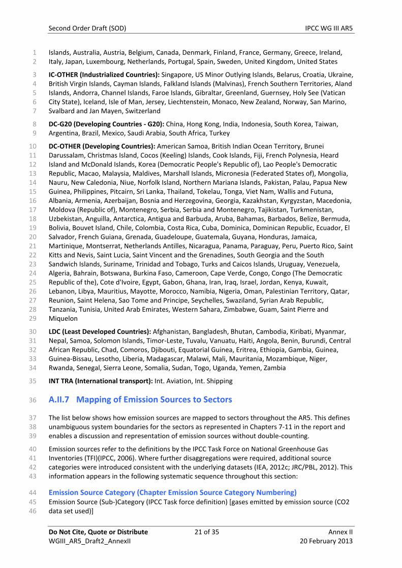
A.II.6.3 ECON5 (Economy-based Aggregation) 44 IC-G20 (Industrialized Countries - G20 and other EU-27): Bulgaria, Cyprus, Czech Republic, Estonia, 45 Hungary, Latvia, Lithuania, Malta, Poland, Romania, Russian Federation, Slovakia, Slovenia, US Virgin 46



Islands, Australia, Austria, Belgium, Canada, Denmark, Finland, France, Germany, Greece, Ireland, 1 Italy, Japan, Luxembourg, Netherlands, Portugal, Spain, Sweden, United Kingdom, United States 2

IC-OTHER (Industrialized Countries): Singapore, US Minor Outlying Islands, Belarus, Croatia, Ukraine, 3 British Virgin Islands, Cayman Islands, Falkland Islands (Malvinas), French Southern Territories, Aland 4 Islands, Andorra, Channel Islands, Faroe Islands, Gibraltar, Greenland, Guernsey, Holy See (Vatican 5 City State), Iceland, Isle of Man, Jersey, Liechtenstein, Monaco, New Zealand, Norway, San Marino, 6 Svalbard and Jan Mayen, Switzerland 7

DC-G20 (Developing Countries - G20): China, Hong Kong, India, Indonesia, South Korea, Taiwan, 8 Argentina, Brazil, Mexico, Saudi Arabia, South Africa, Turkey 9

DC-OTHER (Developing Countries): American Samoa, British Indian Ocean Territory, Brunei 10 Darussalam, Christmas Island, Cocos (Keeling) Islands, Cook Islands, Fiji, French Polynesia, Heard 11 Island and McDonald Islands, Korea (Democratic People's Republic of), Lao People's Democratic 12 Republic, Macao, Malaysia, Maldives, Marshall Islands, Micronesia (Federated States of), Mongolia, 13 Nauru, New Caledonia, Niue, Norfolk Island, Northern Mariana Islands, Pakistan, Palau, Papua New 14 Guinea, Philippines, Pitcairn, Sri Lanka, Thailand, Tokelau, Tonga, Viet Nam, Wallis and Futuna, 15 Albania, Armenia, Azerbaijan, Bosnia and Herzegovina, Georgia, Kazakhstan, Kyrgyzstan, Macedonia, 16 Moldova (Republic of), Montenegro, Serbia, Serbia and Montenegro, Tajikistan, Turkmenistan, 17 Uzbekistan, Anguilla, Antarctica, Antigua and Barbuda, Aruba, Bahamas, Barbados, Belize, Bermuda, 18 Bolivia, Bouvet Island, Chile, Colombia, Costa Rica, Cuba, Dominica, Dominican Republic, Ecuador, El 19 Salvador, French Guiana, Grenada, Guadeloupe, Guatemala, Guyana, Honduras, Jamaica, 20 Martinique, Montserrat, Netherlands Antilles, Nicaragua, Panama, Paraguay, Peru, Puerto Rico, Saint 21 Kitts and Nevis, Saint Lucia, Saint Vincent and the Grenadines, South Georgia and the South 22 Sandwich Islands, Suriname, Trinidad and Tobago, Turks and Caicos Islands, Uruguay, Venezuela, 23 Algeria, Bahrain, Botswana, Burkina Faso, Cameroon, Cape Verde, Congo, Congo (The Democratic 24 Republic of the), Cote d'Ivoire, Egypt, Gabon, Ghana, Iran, Iraq, Israel, Jordan, Kenya, Kuwait, 25 Lebanon, Libya, Mauritius, Mayotte, Morocco, Namibia, Nigeria, Oman, Palestinian Territory, Qatar, 26 Reunion, Saint Helena, Sao Tome and Principe, Seychelles, Swaziland, Syrian Arab Republic, 27 Tanzania, Tunisia, United Arab Emirates, Western Sahara, Zimbabwe, Guam, Saint Pierre and 28 Miquelon 29

LDC (Least Developed Countries): Afghanistan, Bangladesh, Bhutan, Cambodia, Kiribati, Myanmar, 30 Nepal, Samoa, Solomon Islands, Timor-Leste, Tuvalu, Vanuatu, Haiti, Angola, Benin, Burundi, Central 31 African Republic, Chad, Comoros, Djibouti, Equatorial Guinea, Eritrea, Ethiopia, Gambia, Guinea, 32 Guinea-Bissau, Lesotho, Liberia, Madagascar, Malawi, Mali, Mauritania, Mozambique, Niger, 33 Rwanda, Senegal, Sierra Leone, Somalia, Sudan, Togo, Uganda, Yemen, Zambia 34


A.II.7 Mapping of Emission Sources to Sectors 36

The list below shows how emission sources are mapped to sectors throughout the AR5. This defines 37 unambiguous system boundaries for the sectors as represented in Chapters 7-11 in the report and 38 enables a discussion and representation of emission sources without double-counting. 39

Emission sources refer to the definitions by the IPCC Task Force on National Greenhouse Gas 40 Inventories (TFI)(IPCC, 2006). Where further disaggregations were required, additional source 41 categories were introduced consistent with the underlying datasets (IEA, 2012c; JRC/PBL, 2012). This 42 information appears in the following systematic sequence throughout this section: 43

Emission Source Category (Chapter Emission Source Category Numbering) 44

Emission Source (Sub-)Category (IPCC Task force definition) [gases emitted by emission source (CO2 45 data set used)] 46



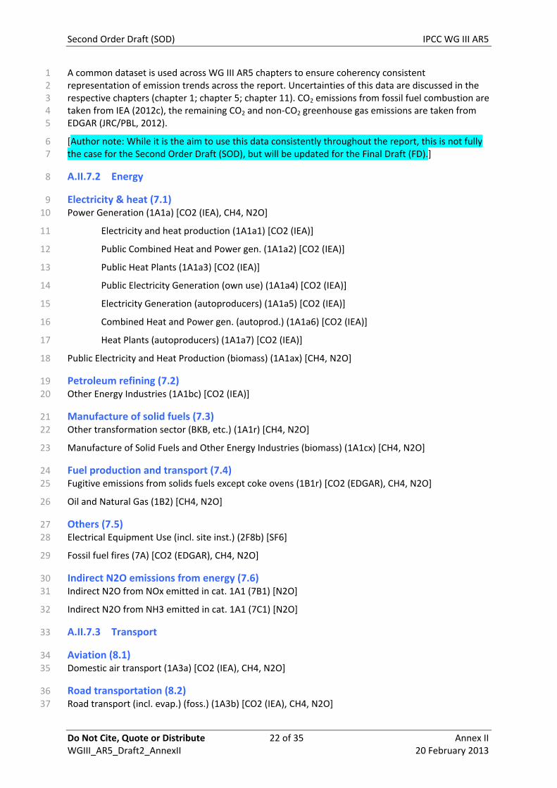
A common dataset is used across WG III AR5 chapters to ensure coherency consistent 1 representation of emission trends across the report. Uncertainties of this data are discussed in the 2 respective chapters (chapter 1; chapter 5; chapter 11). CO2 emissions from fossil fuel combustion are 3 taken from IEA (2012c), the remaining CO2 and non-CO2 greenhouse gas emissions are taken from 4 EDGAR (JRC/PBL, 2012). 5

[Author note: While it is the aim to use this data consistently throughout the report, this is not fully 6 the case for the Second Order Draft (SOD), but will be updated for the Final Draft (FD).] 7

A.II.7.2 Energy 8

Electricity & heat (7.1) 9

Power Generation (1A1a) [CO2 (IEA), CH4, N2O] 10

Electricity and heat production (1A1a1) [CO2 (IEA)] 11

Public Combined Heat and Power gen. (1A1a2) [CO2 (IEA)] 12

Public Heat Plants (1A1a3) [CO2 (IEA)] 13

Public Electricity Generation (own use) (1A1a4) [CO2 (IEA)] 14

Electricity Generation (autoproducers) (1A1a5) [CO2 (IEA)] 15

Combined Heat and Power gen. (autoprod.) (1A1a6) [CO2 (IEA)] 16

Heat Plants (autoproducers) (1A1a7) [CO2 (IEA)] 17

Public Electricity and Heat Production (biomass) (1A1ax) [CH4, N2O] 18

Petroleum refining (7.2) 19

Other Energy Industries (1A1bc) [CO2 (IEA)] 20

Manufacture of solid fuels (7.3) 21

Other transformation sector (BKB, etc.) (1A1r) [CH4, N2O] 22

Manufacture of Solid Fuels and Other Energy Industries (biomass) (1A1cx) [CH4, N2O] 23

Fuel production and transport (7.4) 24

Fugitive emissions from solids fuels except coke ovens (1B1r) [CO2 (EDGAR), CH4, N2O] 25

Oil and Natural Gas (1B2) [CH4, N2O] 26

Others (7.5) 27

Electrical Equipment Use (incl. site inst.) (2F8b) [SF6] 28

Fossil fuel fires (7A) [CO2 (EDGAR), CH4, N2O] 29

Indirect N2O emissions from energy (7.6) 30

Indirect N2O from NOx emitted in cat. 1A1 (7B1) [N2O] 31

Indirect N2O from NH3 emitted in cat. 1A1 (7C1) [N2O] 32

A.II.7.3 Transport 33

Aviation (8.1) 34

Domestic air transport (1A3a) [CO2 (IEA), CH4, N2O] 35

Road transportation (8.2) 36

Road transport (incl. evap.) (foss.) (1A3b) [CO2 (IEA), CH4, N2O] 37



Road transport (incl. evap.) (biomass) (1A3bx) [CH4, N2O] 1

Adiabatic prop.: tyres (2F9b) [SF6] 2

Rail transportation (8.3) 3 Rail transport (1A3c) [CO2 (IEA), CH4, N2O] 4

Non-road transport (rail, etc.) (fos.) (biomass) (1A3cx) [CH4, N2O] 5

Navigation (8.4) 6

Inland shipping (fos.) (1A3d) [CO2 (IEA), CH4, N2O] 7

Inland shipping (fos.) (biomass) (1A3dx) [CH4, N2O] 8

Others incl. indirect N2O emissions from transport (8.5) 9

Non-road transport (fos.) (1A3e) [CO2 (IEA), CH4, N2O] 10

Pipeline transport (1A3e1) [CO2 (IEA)] 11

Non-specified transport (1A3er) [CO2 (IEA)] 12

Non-road transport (fos.) (biomass) (1A3ex) [CH4, N2O] 13

Refrigeration and Air Conditioning Equipment (HFC) (Transport) (2F1a1) [HFC] 14



International Aviation (8.6) 17

Memo: International aviation (1C1) [CO2 (IEA), CH4, N2O] 18

International Shipping (8.7) 19

Memo: International navigation (1C2) [CO2 (IEA), CH4, N2O] 20

A.II.7.4 Buildings 21

Commercial (9.1) 22

Commercial and public services (fos.) (1A4a) [CO2 (IEA), CH4, N2O] 23

Commercial and public services (biomass) (1A4ax) [CH4, N2O] 24

Residential (9.2) 25

Residential (fos.) (1A4b) [CO2 (IEA), CH4, N2O] 26

Residential (biomass) (1A4bx) [CH4, N2O] 27

Others (9.3) 28 Refrigeration and Air Conditioning Equipment (HFC) (Building) (2F1a2) [HFC] 29

Fire Extinguishers (2F3) [PFC] 30

Aerosols/ Metered Dose Inhalers (2F4) [HFC] 31

Adiabatic prop.: shoes and others (2F9a) [SF6] 32

Soundproof windows (2F9c) [SF6] 33

Indirect N2O Emissions from Buildings (9.4) 34





A.II.7.5 Industry 1

Ferrous and non-ferrous metals (10.1) 2

Fuel combustion coke ovens (1A1c1) [CH4, N2O] 3

Blast furnaces (pig iron prod.) (1A1c2) [CH4, N2O] 4

Iron and steel (1A2a) [CO2 (IEA), CH4, N2O] 5

Non-ferrous metals (1A2b) [CO2 (IEA), CH4, N2O] 6

Iron and steel (biomass) (1A2ax) [CH4, N2O] 7

Non-ferrous metals (biomass) (1A2bx) [CH4, N2O] 8

Fuel transformation coke ovens (1B1b1) [CO2 (EDGAR), CH4] 9

Metal Production (2C) [CO2 (EDGAR), CH4, PFC, SF6] 10

Iron and Steel Production (2C1) [CO2 (EDGAR)] 11

Crude steel production total (2C1a) [CO2 (EDGAR)] 12

Blast furnaces (2C1b) [CO2 (EDGAR)] 13

Aluminum production (primary) (2C3) [PFC] 14

SF6 Used in Aluminium and Magnesium Foundries (2C4) [SF6] 15

Magnesium foundries: SF6 use (2C4a) [SF6] 16

Aluminium foundries: SF6 use (2C4b) [SF6] 17

Chemicals (10.2) 18

Chemicals (1A2c) [CO2 (IEA), CH4, N2O] 19

Chemicals (biomass) (1A2cx) [CH4, N2O] 20

Production of chemicals (2B) [CH4, N2O] 21

Production of Halocarbons and SF6 (2E) [HFC, SF6] 22

Other product use (3D) [N2O] 23

Cement production (10.3) 24 Cement production (2A1) [CO2 (EDGAR)] 25

Landfill & waste incineration (10.5) 26

Solid waste disposal on land (6A) [CH4] 27

Waste incineration (6C) [CO2 (EDGAR), CH4, N2O] 28

Other waste handling (6D) [CH4, N2O] 29

Wastewater treatment (10.4) 30

Wastewater handling (6B) [CH4, N2O] 31

Other industries (10.6) 32

Pulp and paper (1A2d) [CO2 (IEA), CH4, N2O] 33

Food and tobacco (1A2e) [CO2 (IEA), CH4, N2O] 34

Other industries (stationary) (fos.) (1A2f) [CO2 (IEA), CH4, N2O] 35

Non-metallic minerals (1A2f1) [CO2 (IEA)] 36



Transport equipment (1A2f2) [CO2 (IEA)] 1

Machinery (1A2f3) [CO2 (IEA)] 2

Mining and quarrying (1A2f4) [CO2 (IEA)] 3

Wood and wood products (1A2f5) [CO2 (IEA)] 4

Construction (1A2f6) [CO2 (IEA)] 5

Textile and leather (1A2f7) [CO2 (IEA)] 6

Non-specified industry (1A2f8) [CO2 (IEA)] 7

Pulp and paper (biomass) (1A2dx) [CH4, N2O] 8

Food and tobacco (biomass) (1A2ex) [CH4, N2O] 9

Off-road machinery: mining (diesel) (1A5b1) [CH4, N2O] 10

Lime production (2A2) [CO2 (EDGAR)] 11

Limestone and Dolomite Use (2A3) [CO2 (EDGAR)] 12

Production of other minerals (2A7) [CO2 (EDGAR)] 13

Refrigeration and Air Conditioning Equipment (PFC) (2F1b) [PFC] 14

Foam Blowing (2F2) [HFC] 15

F-gas as Solvent (2F5) [PFC] 16

Semiconductor Manufacture (2F7a) [HFC, PFC, SF6] 17

Flat Panel Display (FPD) Manufacture (2F7b) [PFC, SF6] 18

Photo Voltaic (PV) Cell Manufacture (2F7c) [PFC] 19

Electrical Equipment Manufacture (2F8a) [SF6] 20

Accelerators/HEP (2F9d) [SF6] 21

Misc. HFCs/SF6 consumption (AWACS, other military, misc.) (2F9e) [SF6] 22

Unknown SF6 use (2F9f) [SF6] 23

Indirect N2O Emissions from Industry (10.7) 24



A.II.7.6 AFOLU 27

Fuel combustion (11.1) 28

Agriculture and forestry (fos.) (1A4c1) [CO2 (IEA), CH4, N2O] 29

Off-road machinery: agric./for. (diesel) (1A4c2) [CH4, N2O] 30

Fishing (fos.) (1A4c3) [CO2 (IEA), CH4, N2O] 31

Non-specified Other Sectors (1A4d) [CO2 (IEA), CH4, N2O] 32

Agriculture and forestry (biomass) (1A4c1x) [CH4, N2O] 33

Fishing (biomass) (1A4c3x) [ , N2O] 34

Non-specified other (biomass) (1A4dx) [CH4, N2O] 35



Livestock (11.2) 1

Enteric Fermentation (4A) [CH4] 2

Manure management (4B) [CH4, N2O] 3

Rice cultivation (11.3) 4

Rice cultivation (4C) [CH4] 5

Direct soil emissions (11.4) 6

CO2 from agricultural lime application (4D4b) [CO2 (EDGAR)] 7

Agricultural soils (direct) (4Dr) [N2O] 8

Forrest fires and decay (11.5) 9

Savanna burning (4E) [CH4, N2O] 10

Forest fires (5A) [CO2 (EDGAR), CH4, N2O] 11

Grassland fires (5C) [CH4, N2O] 12

Forest Fires-Post burn decay (5F2) [CO2 (EDGAR), N2O] 13

Peat fires and decay (11.6) 14

Agricultural waste burning (4F) [CH4, N2O] 15

Peat fires and decay of drained peatland (5D) [CO2 (EDGAR), CH4, N2O] 16

Indirect N2O emissions from AFOLU (11.7) 17

Indirect Emissions (4D3) [N2O] 18

Indirect N2O from NOx emitted in cat. 5 (7B5) [N2O] 19

Indirect N2O from NH3 emitted in cat. 5 (7C5) [N2O] 20

21



References 1

Arvesen A., and E.G. Hertwich (2011). Environmental implications of large-scale adoption of wind 2 power: a scenario-based life cycle assessment. Environmental Research Letters 6, 045102. (DOI: 3 10.1088/1748-9326/6/4/045102). 4

Ayres R.U., and A.V. Kneese (1969). Production, Consumption, and Externalities. American Economic 5 Review 59, 282–297. 6

Ayres R.U., and U.E. Simonis (1994). Industrial Metabolism -- Restructuring for Sustainable 7 Development. United Nations University Press, Tokyo. 8

Baccini P., and P.H. Brunner (1991). Metabolism of the anthroposphere. Springer-Verlag, Berlin; New 9 York, (ISBN: 9780387537788). 10

Berners-Lee M., D.C. Howard, J. Moss, K. Kaivanto, and W.A. Scott (2011). Greenhouse gas 11 footprinting for small businesses - The use of input-output data. Science of the Total Environment 12 409, 883–891. 13

Boulding K. (1972). The Economics of the Coming Spaceship Earth. In: Steady State Economics. H.E. 14 Daly, (ed.), W.H. Freeman, San Francisco pp.121–132, . 15

Boustead I., and G.F. Hancock (1979). Handbook of industrial energy analysis. Ellis Horwood, 16 Chichester, UK. 17

BP (2012). BP Statistical Review of World Energy June 2012. BP, London. Available at: 18 www.bp.com/statisticalreview. 19

Branker K., M.J.M. Pathak, and J.M. Pearce (2011). A review of solar photovoltaic levelized cost of 20 electricity. 15, 4470–4482. 21

Bright R.M., F. Cherubini, and A.H. Strømman (2012). Climate impacts of bioenergy: Inclusion of 22 carbon cycle and albedo dynamics in life cycle impact assessment. Environmental Impact Assessment 23 Review 37, 2–11. (DOI: 10.1016/j.eiar.2012.01.002). 24

Brown R., J. Borgeson, J. Koomey, and P. Biermayer (2008). U.S. Building-Sector Energy Efficiency 25 Potential. Ernest Orlando Lawrence Berkeley National Laboratory, University of California, Berkeley, 26 CA. Available at: http://enduse.lbl.gov/info/LBNL-1096E.pdf. 27

Bullard I., and R.A. Herendeen (1975). The energy cost of goods and services. Energy Pol 3, 268–28 278. 29

Cleveland C.J., R. Costanza, C.A.S. Hall, and R. Kaufmann (1984). Energy and the United-States-30 economy - a biophysical perspective. Science 225, 890–897. 31

Darling S.B., F. You, T. Veselka, and A. Velosa (2011). Assumptions and the levelized cost of energy 32 for photovoltaics. Energy and Environmental Science 4, 3133–3139. 33

Deng L., C.W. Babbitt, and E.D. Williams (2011). Economic-balance hybrid LCA extended with 34 uncertainty analysis: Case study of a laptop computer. Journal of Cleaner Production 19, 1198–1206. 35

Druckman A., P. Bradley, E. Papathanasopoulou, and T. Jackson (2008). Measuring progress 36 towards carbon reduction in the UK. Ecological Economics 66, 594–604. (DOI: 37 10.1016/j.ecolecon.2007.10.020). 38

DTI (2006). Our energy challenge: securing clean, affordable energy for the long term. Department of 39 Trade and Industry, London. Available at: http://www.official-40 documents.gov.uk/document/cm68/6887/6887.pdf. 41



Edenhofer O., R. Pichs, Y. Sokona, K. Seyboth, P. Matschoss, S. Kadner, T. Zwickel, P. Eickemeier, G. 1 Hansen, S. Schlömer, and C. von Stechow (2011). IPCC Special Report on Renewable Energy Sources 2 and Climate Change Mitigation. Cambridge University Press, Cambridge. 3

EERE (2004). Project Financial Evaluation. US Department of Energy, Washington, DC. 4

EIA (2012a). International Energy Statistics. U.S. Energy Information Administration, Washington, 5 D.C. Available at: http://www.eia.gov/cfapps/ipdbproject/IEDIndex3.cfm. 6

EIA (2012b). Annual Energy Review 2011. U.S. Energy Information Administration, Washington, D.C. 7 Available at: http://www.eia.gov/aer. 8

Ekvall T., and B.P. Weidema (2004). System Boundaries and Input Data in Consequential Life Cycle 9 Inventory Analysis. International Journal of Life Cycle Assessment 9, 161–171. 10

Embrechts P., C. Klüppelberg, and T. Mikosch (1997). Modelling Extremal Events for Insurance and 11 Finance. Springer. 12

Erb K., S. Gingrich, F. Krausmann, and H. Haberl (2008). Industrialization, Fossil Fuels, and the 13 Transformation of Land Use. Journal of Industrial Ecology 12, 686–703. (DOI: 10.1111/j.1530-14 9290.2008.00076.x). 15

Erb K.-H., H. Haberl, and C. Plutzar (2012). Dependency of global primary bioenergy crop potentials 16 in 2050 on food systems, yields, biodiversity conservation and political stability. Energy Policy 47, 17 260–269. (DOI: 10.1016/j.enpol.2012.04.066). 18

Finnveden G., M.Z. Hauschild, T. Ekvall, J. Guinee, R. Heijungs, S. Hellweg, A. Koehler, D. 19 Pennington, and S. Suh (2009). Recent developments in Life Cycle Assessment. Journal of 20 Environmental Management 91, 1–21. 21

Fischedick M., R. Schaeffer, A. Adedoyin, M. Akai, T. Bruckner, L. Clarke, V. Krey, I. Savolainen, S. 22 Teske, D. Urge-Vorsatz, R. Wright, and G. Luderer (2011). Chapter 10: Mitigation potential and 23 costs. In: IPCC Special Report on Renewable Energy Sources and Climate Change Mitigation. 24 Cambridge University Press, Cambridge. 25

Fischer-Kowalski M., and H. Haberl (1997). Tons, Joules and Money: Modes of Production and their 26 Sustainability Problems. Society & Natural Resources 10, 61–85. 27

Fischer-Kowalski M., and H. Haberl (2007). Socioecological Transitions and Global Change. 28 Trajectories of Social Metabolism and Land Use. E.Elgar, Cheltenham, UK. 29

Fisher B.S., N. Nakicenovic, K. Alfsen, J. Corfee Morlot, F. de la Chesnaye, J.-C. Hourcade, K. Jiang, 30 M. Kainuma, E. La Rovere, A. Matysek, A. Rana, K. Riahi, R. Richels, S. Rose, D. van Vuuren, and R. 31 Warren (2007). Issues related to mitigation in the long term context. In: Climate Change 2007: 32 Mitigation. Contribution of Working Group III to the Fourth Assessment Report of the Inter-33 governmental Panel on Climate Change. Cambridge University Press, Cambridge, UK. 34

Gandhi N., M.L. Diamond, D. van de Meent, M.A.J. Huijbregts, W.J.G.M. Peijnenburg, and J. 35 Guinee (2010). New Method for Calculating Comparative Toxicity Potential of Cationic Metals in 36 Freshwater: Application to Copper, Nickel, and Zinc. Environmental Science & Technology 44, 5195–37 5201. (DOI: 10.1021/es903317a). 38

Girod B., P. de Haan, and R.W. Scholz (2011). Consumption-as-usual instead of ceteris paribus 39 assumption for demand. International Journal of Life Cycle Assessment 16, 3–11. (DOI: 40 10.1007/s11367-010-0240-z). 41

Graedel T.E., and J. Cao (2010). Metal spectra as indicators of development. Proceedings of the 42 National Academy of Sciences 107, 20905–20910. (DOI: 10.1073/pnas.1011019107). 43



Greening L.A., M. Ting, and T.J. Krackler (2001). Effects of changes in residential end-uses and 1 behavior on aggregate carbon intensity: comparison of 10 OECD countries for the period 1970 2 through 1993. Energy Economics 23, 153–178. 3

Grübler A., M. Jefferson, and N. Nakićenović (1996). Global energy perspectives: A summary of the 4 joint study by the international institute for applied systems analysis and world energy council. 5 Technological Forecasting and Social Change 51, 237–264. (DOI: 10.1016/0040-1625(95)00251-0). 6

Grubler A., T.B. Johansson, L. Mundaca, N. Nakicenovic, S. Pachauri, K. Riahi, H.-H. Rogner, L. 7 Strupeit, P. Kolp, V. Krey, J. Macknick, Y. Nagai, M.L. Rogner, K.R. Smith, K. Steen-Olsen, and J. 8 Weinzettel (2012). Energy Primer. In: The Global Energy Assessment: Toward a More Sustainable 9 Future. IIASA, Laxenburg, Austria and Cambridge University Press, Cambridge, UK, .Available at: 10 http://www.iiasa.ac.at/web/home/research/researchPrograms/Energy/Chapter1.en.html. 11

12 (2010). Life Cycle Assessment: Past, Present, and Future. Environmental Science & Technology 45, 13 90–96. (DOI: 10.1021/es101316v). 14

Gustavsson L., K. Pingoud, and R. Sathre (2006). Carbon Dioxide Balance of Wood Substitution: 15 Comparing Concrete- and Wood-Framed Buildings. Mitigation and Adaptation Strategies for Global 16 Change 11, 667–691. (DOI: 10.1007/s11027-006-7207-1). 17

Haas R., and L. Schipper (1998). Residential energy demand in OECD-countries and the role of 18 irreversible efficiency improvements. Energy Econ 20, 421–442. 19

Haberl H. (2001a). The Energetic Metabolism of Societies Part I: Accounting Concepts. Journal of 20 Industrial Ecology 5, 11–33. (DOI: 10.1162/108819801753358481). 21

Haberl H. (2001b). The Energetic Metabolism of Societies: Part II: Empirical Examples. Journal of 22 Industrial Ecology 5, 71–88. (DOI: 10.1162/10881980152830141). 23

Haberl H., K.-H. Erb, F. Krausmann, A. Bondeau, C. Lauk, C. Müller, C. Plutzar, and J.K. Steinberger 24 (2011). Global bioenergy potentials from agricultural land in 2050: Sensitivity to climate change, 25 diets and yields. Biomass and Bioenergy 35, 4753–4769. (DOI: 16/j.biombioe.2011.04.035). 26

Haberl H., K.H. Erb, F. Krausmann, V. Gaube, A. Bondeau, C. Plutzar, S. Gingrich, W. Lucht, and M. 27 Fischer-Kowalski (2007). Quantifying and mapping the human appropriation of net primary 28 production in earth’s terrestrial ecosystems. Proceedings of the National Academy of Sciences 104, 29 12942 –12947. (DOI: 10.1073/pnas.0704243104). 30

Haberl H., M. Fischer-Kowalski, F. Krausmann, H. Weisz, and V. Winiwarter (2004). Progress 31 towards sustainability? What the conceptual framework of material and energy flow accounting 32 (MEFA) can offer. Land Use Policy 21, 199–213. (DOI: 16/j.landusepol.2003.10.013). 33

Haberl H., H. Weisz, C. Amann, A. Bondeau, N. Eisenmenger, K. Erb, M. Fischer‐Kowalski, and F. 34 Krausmann (2006). The Energetic Metabolism of the European Union and the United States: Decadal 35 Energy Input Time‐Series with an Emphasis on Biomass. Journal of Industrial Ecology 10, 151–171. 36 (DOI: 10.1162/jiec.2006.10.4.151). 37

Hannon B., R. Costanza, and R.A. Herendeen (1986). Measures of Energy-Cost and Value in 38 Ecosystems. Journal of Environmental Economics and Management 13, 391–401. 39

Hannon B., R.G. Stein, B.Z. Segal, and D. Serber (1978). Energy and Labor in the Construction Sector. 40 Science 202, 837–847. 41

Hansen S. (2012). Economical optimization of building elements for use in design of nearly zero 42 energy buildings. In Proceedings: Proceedings of the 5th IBPC. Kyoto, Japan. 28-May-2012, .Available 43 at: http://orbit.dtu.dk/fedora/objects/orbit:113660/datastreams/file_10074204/content. 44



Heptonstall (2007). Review of Electricity Unit Cost Estimates. UK Energy Research Centre, London. 1 Available at: 2 http://data.ukedc.rl.ac.uk/browse/edc/Electricity/ProductionCostEstimates/Heptonstall2007_Worki3 ngPaper.pdf. 4

Hertwich E.G. (2011). The life cycle environmental impacts of consumption. Economic Systems 5 Research 23, 27–47. (DOI: 10.1080/09535314.2010.536905). 6

Hertwich E.G., and G.P. Peters (2009). Carbon footprint of nations: A global, trade-linked analysis. 7 Environmental Science & Technology 43, 6414–6420. 8

Huijbregts M., W. Schöpp, E. Verkuijlen, R. Heijungs, and L. Reijnders (2000). Spatially explicity 9 characterization of acidifying and eutrophying air pollution in life-cycle assessment. J. Ind. Ecol. 4, 10 125–142. 11

IEA (2012a). Energy Balances of OECD Countries. International Energy Agency, Paris, (ISBN: 978-92-12 64-17382-8). 13

IEA (2012b). Energy Balances of Non-OECD Countries. International Energy Agency, Paris, (ISBN: 978-14 92-64-17466-5). 15

IEA (2012c). CO2 Emissions from Fuel Combustion. Beyond 2020 Online Database. Available at: 16 http://data.iea.org. 17

IEA, and NEA (2005). Projected Costs of Generating Electricity. NEA/IEA/OECD, Paris. 18

IEA/OECD/Eurostat (2005). Energy Statistics Manual. OECD/IEA, Paris. Available at: 19 http://www.iea.org/stats/docs/statistics_manual.pdf. 20

Imhoff M.L., L. Bounoua, T. Ricketts, C. Loucks, R. Harriss, and W.T. Lawrence (2004). Global 21 patterns in human consumption of net primary production. Nature 429, 870–873. (DOI: 22 10.1038/nature02619). 23

IPCC (2001). Climate Change 2001: Mitigation Appendices - IV Units, Conversion Factors, and GDP 24 Deflators. In: Climate Change 2001: Mitigation; Contribution of Working Group III to the Third 25 Assessment Report of the IPCC. Cambridge University Press, Cambridge pp.727–732, (ISBN: ISBN 0-26 521-01502-2). 27

IPCC (Ed.) (2006). IPCC Guidelines for National Greenhouse Gas Inventories. IGES, Japan. 28

Joskow P.L. (2011). Comparing the costs of intermittent and dispatchable electricity generating 29 technologies. American Economic Review 101, 238–241. 30

JRC/PBL (2012). European Commission, Joint Research Centre (JRC)/PBL Netherlands Environmental 31 Assessment Agency. Emission Database for Global Atmospheric Research (EDGAR). Available at: 32 http://edgar.jrc.ec.europa.eu. 33

Kato K., A. Murata, and K. Sakuta (1998). Energy pay-back time and life-cycle CO2 emission of 34 residential PV power system with silicon PV module. Progress in Photovoltaics 6, 105–115. 35

Kousky C., and R. Cooke (2009). The Unholy Trinity: Fat Tails, Tail Dependence, and Micro-36 Correlations. Resources for the Future (RFF), Washington, DC. Available at: 37 http://www.ncsu.edu/cenrep/workshops/TREE/documents/Kousky_RFF_paper.pdf. 38

Krausmann F., K.-H. Erb, S. Gingrich, C. Lauk, and H. Haberl (2008). Global patterns of 39 socioeconomic biomass flows in the year 2000: A comprehensive assessment of supply, 40 consumption and constraints. Ecological Economics 65, 471–487. (DOI: 16/j.ecolecon.2007.07.012). 41

Krausmann F., S. Gingrich, N. Eisenmenger, K.-H. Erb, H. Haberl, and M. Fischer-Kowalski (2009). 42 Growth in global materials use, GDP and population during the 20th century. Ecological Economics 43 68, 2696–2705. (DOI: 16/j.ecolecon.2009.05.007). 44



Lan J., M. Lenzen, E. Dietzenbacher, D. Moran, K. Kanemoto, J. Murray, and A. Geschke (2012). 1 Structural Change and the Environment. Journal of Industrial Ecology 16, 623–635. (DOI: 2 10.1111/j.1530-9290.2012.00518.x). 3

Larsen H.N., and E.G. Hertwich (2009). The case for consumption-based accounting of greenhouse 4 gas emissions to promote local climate action. Environmental Science and Policy 12, 791–798. 5

Larson E.D., Z. Li, and R.H. Williams (2012). Chapter 12 - Fossil Energy. In: Global Energy Assessment 6 - Toward a Sustainable Future.Cambridge University Press, Cambridge, UK and New York, NY, USA 7 and the International Institute for Applied Systems Analysis, Vienna, Austria pp.901–992, (ISBN: 8 9780521182935). 9

Lauk C., H. Haberl, K.H. Erb, S. Gingrich, and F. Krausmann (2012). Global socioeconomic carbon 10 stocks and carbon sequestration in long-lived products 1900-2008. Environmental Research Letters 11 in review. 12

Lenzen M. (2001). Errors in conventional and input-output-based life-cycle inventories. Journal of 13 Industrial Ecology 4, 127–148. 14

Lenzen M., C. Dey, and B. Foran (2004). Energy requirements of Sydney households. Ecol. Econ. 49, 15 375–399. 16

Lenzen M., K. Kanemoto, D. Moran, and A. Geschke (2012). Mapping the Structure of the World 17 Economy. Environmental Science & Technology 46, 8374–8381. (DOI: 10.1021/es300171x). 18

Lenzen M., and R. Schaeffer (2004). Environmental and social accounting for Brazil. Environ. Resour. 19 Econ. 27, 201–226. 20

Leontief W.W. (1936). Quantitative input and output relations in the economic system of the United 21 States. Rev. Econ. Stat. 18, 105–125. 22

Leontief W. (1971). Environment and Economic Structure. Analyse Et Prevision 11, 253–276. 23

Lightfoot H.D. (2007). Understand the three different scales for measuring primary energy and avoid 24 errors. Energy 32, 1478–1483. 25

Liu G., C.E. Bangs, and D.B. Müller (2011). Unearthing Potentials for Decarbonizing the U.S. 26 Aluminum Cycle. Environ. Sci. Technol. 45, 9515–9522. (DOI: 10.1021/es202211w). 27

Liu G., C.E. Bangs, and D.B. Müller (2012). Stock dynamics and emission pathways of the global 28 aluminium cycle. Nature Climate Change Advance online publication. (DOI: 10.1038/nclimate1698). 29 Available at: http://www.nature.com/nclimate/journal/vaop/ncurrent/full/nclimate1698.html. 30

Macknick J. (2011). Energy and CO2 emission data uncertainties. Carbon Management 2, 189–205. 31

Majeau-Bettez G., A.H. Strømman, and E.G. Hertwich (2011). Evaluation of process- and input-32 output-based life cycle inventory data with regard to truncation and aggregation issues. 33 Environmental Science and Technology 45, 10170–10177. 34

Martinez-Alier J. (1987). Ecological Economics. Energy, Environment and Society. Blackwell, Oxford, 35 UK. 36

Martinot E., C. Dienst, L. Weiliang, and C. Qimin (2007). Renewable Energy Futures: Targets, 37 Scenarios, and Pathways. Annual Review of Environment and Resources 32, 205–239. (DOI: 38 10.1146/annurev.energy.32.080106.133554). 39

Meier A. (1983). The cost of conserved energy as an investment statistic. Heating, Piping, and Air 40 Conditioning 55, 73–77. 41



Melaina M., and K. Webster (2011). Role of Fuel Carbon Intensity in Achieving 2050 Greenhouse 1 Gas Reduction Goals within the Light-Duty Vehicle Sector. Environmental Science & Technology 45, 2 3865–3871. (DOI: 10.1021/es1037707). 3

Miller R.E., and P.D. Blair (1985). Input-output analysis: Foundations and extensions. Prentice-Hall, 4 Englewood Cliffs, NJ. 5

Minx J.C., T. Wiedmann, R. Wood, G.P. Peters, M. Lenzen, A. Owen, K. Scott, J. Barrett, K. Hubacek, 6 G. Baiocchi, A. Paul, E. Dawkins, J. Briggs, D. Guan, S. Suh, and F. Ackerman (2009). INPUT-OUTPUT 7 ANALYSIS AND CARBON FOOTPRINTING: AN OVERVIEW OF APPLICATIONS. Economic Systems 8 Research 21, 187–216. (DOI: 10.1080/09535310903541298). 9

Moomaw W., P. Burgherr, G. Heath, M. Lenzen, J. Nyboer, and A. Verbruggen (2011). Annex II: 10 Methodology. In: IPCC Special Report on Renewable Energy Sources and Climate Change Mitigation. 11 Cambridge University Press, Cambridge. 12

Morita T., J. Robinson, A. Adegbulugbe, J. Alcamo, D. Herbert, E. Lebre la Rovere, N. Nakicenivic, H. 13 Pitcher, P. Raskin, K. Riahi, A. Sankovski, V. Solkolov, B. de Vries, and D. Zhou (2001). Greenhouse 14 gas emission mitigation scenarios and implications. In: Climate Change 2001: Mitigation; 15 Contribution of Working Group III to the Third Assessment Report of the IPCC. Cambridge University 16 Press, Cambridge pp.115–166, (ISBN: ISBN 0-521-01502-2). 17

Müller D.B. (2006). Stock dynamics for forecasting material flows--Case study for housing in The 18 Netherlands. Ecological Economics 59, 142–156. 19

Müller D.B., T. Wang, B. Duval, and T.E. Graedel (2006). Exploring the engine of anthropogenic iron 20 cycles. Proceedings of the National Academy of Sciences 103, 16111 –16116. (DOI: 21 10.1073/pnas.0603375103). 22

Nakamura S., and Y. Kondo (2001). Input-Output Analysis of Waste Management. J. Ind. Ecol. 6, 39–23 64. 24

Nakamura S., K. Nakajima, Y. Kondo, and T. Nagasaka (2007). The waste input-output approach to 25 materials flow analysis - Concepts and application to base metals. Journal of Industrial Ecology 11, 26 50–63. 27

Nakicenovic N., A. Grubler, and A. McDonald (1998). Global Energy Perspectives. Cambridge 28 University Press, Cambridge. 29

Nakicenovic N., and R. Swart (2000). IPCC Special Report on Emissions Scenarios. Cambridge 30 University Press, Cambridge. 31

NAS (2007). Coal: Research and Development to Support National Energy Policy (Committee on Coal 32 Research and Technology and National Research Council, Eds.). The National Academies Press, (ISBN: 33 9780309110228). Available at: http://www.nap.edu/openbook.php?record_id=11977. 34

Nordhaus W.D. (2006). The “Stern Review” on the Economics of Climate Change. SSRN eLibrary. 35 Available at: http://papers.ssrn.com/sol3/papers.cfm?abstract_id=948654. 36

Norris G.A. (2002). Life cycle emission distributions within the economy: Implications for life cycle 37 impact assessment. Risk Analysis 22, 919–930. 38

Pauliuk S., N.M.A. Dhaniati, and D. Müller (2011). Reconciling Sectoral Abatement Strategies with 39 Global Climate Targets: The Case of the Chinese Passenger Vehicle Fleet. Environ. Sci. Technol. (DOI: 40 10.1021/es201799k). Available at: http://dx.doi.org/10.1021/es201799k. 41

Pauliuk S., K. Sjöstrand, and D.B. Müller (2012). Transforming the dwelling stock to reach the 2°C 42 climate target – combining MFA and LCA models for a case study on Norway. Journal of Industrial 43 Ecology In press. 44



Peters G.P. (2010). Carbon footprints and embodied carbon at multiple scales. Current Opinion in 1 Environmental Sustainability 2, 245–250. (DOI: 10.1016/j.cosust.2010.05.004). 2

Peters G.P., B. Aamaas, M. T. Lund, C. Solli, and J.S. Fuglestvedt (2011). Alternative “Global 3 Warming” Metrics in Life Cycle Assessment: A Case Study with Existing Transportation Data. 4 Environmental Science & Technology 45, 8633–8641. (DOI: 10.1021/es200627s). 5

Peters G.P., and E.G. Hertwich (2008). CO2 embodied in international trade with implications for 6 global climate policy. Environmental Science and Technology 42, 1401–1407. 7

Peters G.P., J.C. Minx, C.L. Weber, and O. Edenhofer (2011). Growth in emission transfers via 8 international trade from 1990 to 2008. Proceedings of the National Academy of Sciences of the 9 United States of America 108, 8903–8908. (DOI: 10.1073/pnas.1006388108). 10

Portney P., and J.P. Weyant (1999). Discounting and intergenerational equity. RFF Press, (ISBN: 11 0915707896). 12

Short W., D.J. Packey, and T. Holt (1995). A Manual for the Economic Evaluation of Energy Efficiency 13 and Renewable Energy Technologies. NREL. 14

Sorrell S., and J. Dimitropoulos (2008). The rebound effect: Microeconomic definitions, limitations 15 and extensions. Ecological Economics 65, 636–649. (DOI: 10.1016/j.ecolecon.2007.08.013). 16

Stern N. (2007). The Economics of Climate Change: The Stern Review. Cambridge University Press, 17 712 pp. Available at: http://www.hm-18 treasury.gov.uk/independent_reviews/stern_review_economics_climate_change/stern_review_rep19 ort.cfm. 20

Stromman A.H., E.G. Hertwich, and F. Duchin (2009). Shifting Trade Patterns as a Means of 21 Reducing Global Carbon Dioxide Emissions. Journal of Industrial Ecology 13, 38–57. (DOI: 22 10.1111/j.1530-9290.2008.00084.x). 23

Suerkemper F., S. Thomas, D. Osso, and P. Baudry (2012). Cost-effectiveness of energy efficiency 24 programmes-evaluating the impacts of a regional programme in France. Energy Efficiency 5, 121–25 135. 26

Suh S., M. Lenzen, G.J. Treloar, H. Hondo, A. Horvath, G. Huppes, O. Jolliet, U. Klann, W. Krewitt, Y. 27 Moriguchi, J. Munksgaard, and G. Norris (2004). System Boundary Selection in Life-Cycle Inventories 28 Using Hybrid Approaches. Environ. Sci. Technol. 38, 657 –664. 29

Takase K., Y. Kondo, and A. Washizu (2005). An analysis of sustainable consumption by the waste 30 input-output model. Journal of Industrial Ecology 9, 201–220. 31

Treloar G. (1996). Extracting embodied energy paths from input-output tables: towards an input-32 output-based hybrid energy analysis method. Econ. Systems Res. 9, 375–391. 33

Tukker A., A. de Koning, R. Wood, T. Hawkins, S. Lutter, J. Acosta, J.M. Rueda Cantuche, M. 34 Bouwmeester, J. Oosterhaven, T. Drosdowski, and J. Kuenen (2013). EXIOPOL - development and 35 illustrative analyses of detailed global multiregional, environmentally extended supply and use 36 tables and symmetric input-output tables. Economic Systems Research 25, in press. (DOI: 37 10.1080/09535314.2012.761953). 38

Turkenburg W.C., D. Arent, R. Bertani, A. Faaij, M. Hand, W. Krewitt, E.D. Larson, J. Lund, M. 39 Mehos, T. Merrigan, C. Mitchell, J.R. Moreira, W. Sinke, V. Sonntag-O’Brien, B. Thresher, W. van 40 Sark, and E. Usher (2012). Chapter 11 - Renewable Energy. In: Global Energy Assessment - Toward a 41 Sustainable Future.Cambridge University Press, Cambridge, UK and New York, NY, USA and the 42 International Institute for Applied Systems Analysis, Vienna, Austria pp.761–900, (ISBN: 43 9780521182935). Available at: 44 http://www.iiasa.ac.at/web/home/research/researchPrograms/Energy/Chapte11.en.html. 45



Turner K., M. Lenzen, T. Wiedmann, and J. Barrett (2007). Examining the global environmental 1 impact of regional consumption activities - Part 1: A technical note on combining input-output and 2 ecological footprint analysis. Ecological Economics 62, 37–44. (DOI: 3 10.1016/j.ecolecon.2006.12.002). 4

UN Statistics (2010). Energy Balances and Electricity Profiles - Concepts and definitions. Available at: 5 http://unstats.un.org/unsd/energy/balance/concepts.htm. 6

UNEP (2012). Global Trends in Renewable Energy Investment 2012. UNEP, Frankfurt School of 7 Finance and Management, Bloomberg New Energy Finance. Available at: http://fs-unep-8 centre.org/sites/default/files/publications/globaltrendsreport2012final.pdf. 9

Ürge-Vorsatz D. (1996). Exploring US residential and commercial electricity conservation potentials: 10 analysis of the lighting sector. University of California, Los Angeles, CA. 11

Viebahn P., Y. Lechon, and F. Trieb (2011). The potential role of concentrated solar power (CSP) in 12 Africa and Europe-A dynamic assessment of technology development, cost development and life 13 cycle inventories until 2050. Energy Policy 39, 4420–4430. 14

Vitousek P.M., P.R. Ehrlich, A.H. Ehrlich, and P.A. Matson (1986). Human Appropriation of the 15 Products of Photosynthesis. Bioscience 36, 363–373. 16

Vizcarra A.T., K.V. Lo, and P.H. Liao (1994). A life-cycle inventory of baby diapers subject to canadian 17 conditions. Environmental Toxicology And Chemistry 13, 1707–1716. 18

Watson R., M.C. Zinyowera, and R. Moss (1995). Climate Change 1995. Impacts, Adaptations and 19 Mitigation of Climate Change: Scientific Analyses. Contribution of Working Group II to the Second 20 Assessment Report of the Intergovernmental Panel on Climate Change. Cambridge University Press, 21 Cambridge, 861 pp. 22

WEC (1993). Energy for Tomorrow’s World. WEC Commission global report. London, UK. 23

Weisz H., F. Krausmann, C. Amann, N. Eisenmenger, K.-H. Erb, K. Hubacek, and M. Fischer-Kowalski 24 (2006). The physical economy of the European Union: Cross-country comparison and determinants 25 of material consumption. Ecological Economics 58, 676–698. (DOI: 16/j.ecolecon.2005.08.016). 26

Wiedmann T., and J. Minx (2008). A Definition of “carbon footprint”. In: Ecological Economics 27 Research Trends. Nova Sci., New York pp.1–11, (ISBN: 1-60021-941-1). Available at: http://www.isa-28 research.co.uk/docs/ISA-UK_Report_07-01_carbon_footprint.pdf. 29

Wiedmann T., H.C. Wilting, M. Lenzen, S. Lutter, and V. Palm (2011). Quo Vadis MRIO? 30 Methodological, data and institutional requirements for multi-region input–output analysis. Special 31 Section - Earth System Governance: Accountability and Legitimacy 70, 1937–1945. (DOI: 32 10.1016/j.ecolecon.2011.06.014). 33

Wiedmann T., R. Wood, J.C. Minx, M. Lenzen, D.B. Guan, and R. Harris (2010). A Carbon Footprint 34 Time Series of the UK - Results from a Multi-Region Input-Output Model. Economic Systems Research 35 22, 19–42. (DOI: 10.1080/09535311003612591). 36

Williams E.D., C.L. Weber, and T.R. Hawkins (2009). Hybrid framework for managing uncertainty in 37 life cycle inventories. Journal of Industrial Ecology 13, 928–944. 38

Wolman A. (1965). The metabolism of cities. Scientific American 213, 179–190. 39

World Bank (2013). World Development Indicators (WDI) Database. World Bank, Washington, DC. 40 Available at: http://data.worldbank.org/data-catalog/world-development-indicators. 41

Wright D.H. (1990). Human Impacts on Energy Flow through Natural Ecosystems, and Implications 42 for Species Endangerment. Ambio 19, 189–194. 43



Wyckoff A.W., and J.M. Roop (1994). The Embodiment of Carbon in Imports of Manufactured 1 Products - Implications for International Agreements on Greenhouse-Gas Emissions. Energy Policy 2 22, 187–194. 3

Xu M., B. Allenby, and W.Q. Chen (2009). Energy and Air Emissions Embodied in China-US Trade: 4 Eastbound Assessment Using Adjusted Bilateral Trade Data. Environmental Science & Technology 43, 5 3378–3384. (DOI: 10.1021/es803142v). 6

Zamagni A., J. Guinée, R. Heijungs, P. Masoni, and A. Raggi (2012). Lights and shadows in 7 consequential LCA. International Journal of Life Cycle Assessment 17, 904–918. 8

9

AR5 SOD Chapter 18

Documents

Transcript of AR5 SOD Chapter 18