Articulated body

dynamics

Articulated rigid bodies

Beyond human models

Quadraped animals

Wavy hair

Animal fur

Plants

How would you represent a pose?

Maximal vs. reduced coordinates

(x0,R0)

(x1,R1)

(x2,R2)

Maximal coordinates

Assuming there are m links and n DOFs in the articulated body, how many constraints do we need to keep links connected correctly in maximal coordinates?

Reduced coordinates

θ0, φ0, ψ0

θ1, φ1

θ2

state variables: 6m state variables: n

How are things connected?

Maximal coordinate

Treat each body part as a separate rigid body

Use explicit constraints to connect body parts

Reduced coordinate

Use joint angles directly as state variables

Hard to derive the equation of motion for articulated bodies

Maximal coordinates

Direct extension of well understood rigid body dynamics; easy to understand and implement

Operate in Cartesian space; hard to

evaluate joint angles and velocities

enforce joint limits

apply internal joint torques

Inaccuracy in numeric integration can cause body parts to drift apart

Reduced coordinates

Joint space is more intuitive when dealing with complex multi-body structures

Fewer DOFs and fewer constraints

Well suited for character motion and motion control

Forward simulation

Given current state, current velocity, external forces, and

joint torques, compute the current acceleration of the

articulated body

Lagrangian method

Featherstone’s algorithm

Use reduced coordinates to represent motion

Given the current joint , current joint velocity , external forces and joint torque , compute the joint acceleration in linear time

Featherstone’s algorithm

q q

q

FE

G

q = f(q, q,FE ,G)

link i

link λ(i)joint i connects link i and its parent

Spatial notation

Spatial notation combines linear and angular quantities

Two ordinary 3-dimensional vectors are replaced by a

single 6-dimensional spatial vector

v =

[

ω

x

]

a =

[

ω

x

]

angular velocity of the body

linear velocity of the body

Spatial velocity of each link

If we let be the velocity of link i, and be the velocity

across joint i then

vi vJi

vJi = vi − vλ(i)

vJi = hiqi

The joint velocity can also be described in the form

where hi is a 6 by di matrix, is a di by 1 vector and di is the

degree of freedom of joint i

q

Spatial acceleration of each link

ai = aλ(i) + hiqi + hiqi

vi = vλ(i) + hiqi

Velocity of link i:

Acceleration of link i:

Newton-Euler equations

fi + fE

i = Iiai + vi × Iivi

Equation of motion for link i:

net force applied to link

i through the joints

sum of all other forces

actin on link i

fi = fJi −

∑

j∈µ(i)

fJj

fJi is the force transmitted from link λ(i)

µ(i) is the set of children of link i

fJi = Iiai + vi × Iivi − f

Ei +

∑

j∈µ(i)

fJj

Acceleration-force relation

The acceleration of bodies are always linear functions of

the applied forces

a = Φf + b

f = IAa + pA

The equation can be inverted to

IA articulated body inertia

pA

bias force, the force required to bring the body’s

acceleration to zero

IA

= Φ−1where

pA= −IAb

Featherstone’s algorithm

q, q,FE,Gproc ABM_accelerations( )

/* first outbound loop */

/* inbound loop */

/* second outbound loop */

Compute_Inertia_Bias();

Compute_joint_accel();

vi = vλ(i) + hiqi

for i = 1 to N - 1

v0 = 0

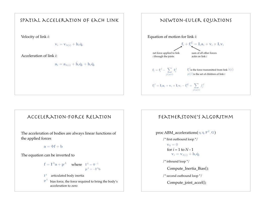
Inbound loop

Starting at the terminal links, calculate the inertia and

bias force for each link in turn

IAi = Ii +

∑

j∈µ(i)

(IAj − I

Aj hj(h

Tj I

Aj hj)

−1h

Tj I

Aj )

pAi = pi +

∑

j∈µ(i)

(pαj + IA

j hj(hTj IA

j hj)−1(Gi − hT

j pαj ))

pi = vi × Iivi − fE

i

pαj = pA

j + IAj hjqj

wherefJi = Iiai + vi × Iivi − f

Ei +

∑

j∈µ(i)

fJj

Second outbound loop

fJi = IA

i ai + pAi

τi = hTi f

Ji

qi = (hTi IA

i hi)−1(τi − hT

i (IAi aλ(i) + pα

i ))

Compute joint acceleration from the root to the terminal

link

for i = 0 to N-1

τ0 = 0

ai = aλ(i) + hiqi + hiqi

aλ(0) = 0

Lagrangian method

d

dt

∂T

∂qj

−

∂T

∂qj

− Qj = 0

j is the index for DOFs in generalized coordinates

Qj is the generalized force associated with coordinate j

T denotes the kinetic energy

Generalized coordinates

The configuration of a multi-body system is identify by a set of variables called generalized coordinates

articulated bodies: θ0, φ0, ψ0

θ1, φ1

θ2

x, y, z,

x, y, z, θ, φ, ψone rigid body:

one particle: x, y, z

These generalized coordinates are independent and completely determine the location and orientation of each body in the system

Peaucellier mechanism

The purpose of this mechanism is to generate a straight-line motion

This mechanism has eight bodies and yet the number of degrees of freedom is one

Generalized forces

δri =∂ri

∂q1

δq1 +∂ri

∂q2

δq2 + . . . +∂ri

∂qn

δqn =

∑

j

∂ri

∂qj

δqj

Fiδri = Fi

∑

j

∂ri

∂qj

δqj =

∑

j

Qjδqj

ri = ri(q1, q2, . . . , qn)

Represent a point ri on the articulated body system by a set of generalized coordinates:

The virtual displacement of ri can be written in terms of generalized coordinates

The virtual work of force Fi acting on ri is

Qj = Fi ·∂ri

∂qj

Define generalized force associated with coordinate qj

Kinetic energy

r = Wr0

Ti =1

2

∫r

T

0 WT

i Wir0τi dx dy dz

Ti =1

2

∫

tr

(

Wir0rT

0 WT

i

)

τi dx dy dz

Ti =1

2

∫r

Trτi dx dy dz

Ti =1

2tr

(

Wi

[∫

r0rT

0 τi dx dy dz

]

WT

i

)

Ti =1

2tr

(

WiMiWT

i

)

Mi =

∫r0r

T

0 τi dx dy dz

Compute and by yourself∂Ti

∂qj

d

dt

∂Ti

∂qj

Lagrangian method

d

dt

∂Ti

∂qj

−

∂Ti

∂qj

= tr

(

∂Wi

∂qj

MiWTi

)

= Qj

Put it all together

tr

(

∂Wi

∂qjMiW

Ti

)

=

∑

k

fk∂pk

∂qj

Represent external forces fk in terms of generalized coordinates

where fk is acting at the point pk on the articulated body system

Acceleration of transformation

Wi = Wi−1Ri

Wi = Wi−1Ri + Wi−1Ri

Wi = Wi−1Ri + 2Wi−1RiWi−1Ri

R(q) =

Represent in terms of , and W(q) q q q

Compute recursivelyW(q)

Constraints

Penalty methods

Use proportional derivative (PD) controllers

Analytical methods

Solve a linear system

Acceleration constraints

Given a desired joint acceleration , what is the torque that gives rise to it?

qt= kgt

+ q0 k =qt

− q0

gt

1. Use test torque to computegt

k

gc

= gtq

c− q

0

qt− q0

2. Use to compute the desired joint torquek gc

af= kf + a0

Force - Acceleration relationship

h(qf ) − h(q0) = kf

qc

Multiple constraints

Compute the force magnitudes that satisfy all the acceleration constraints simultaneously

f

h1(q) − h1(q0) = k11f1 + k12f2 + · · · + k1mfm

hm(q) − hm(q0) = km1f1 + km2f2 + · · · + kmmfm

h2(q) − h2(q0) = k21f1 + k22f2 + · · · + k2mfm

.

.

.

h − h0

= Kf

kji =1

f ti

(hj(qti) − hj(q

0))

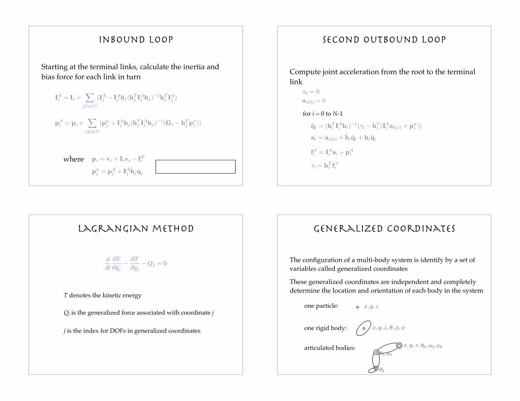
Impact constraints

Use impulse to instantaneously change the body’s velocities

p

Compute the current joint velocities,

! that changes the velocity of body

point instantaneously from top

q

v+p

v−

p

v+p

v−

p

Impact constraints

ap = (v+p− v−

p)/δt

Compute desired acceleration on the body point

h(q) = a(q) − ap

fp

Find the appropriate constraint magnitude that

satisfy the acceleration constraint

q0

qp

Evaluate the default joint acceleration, ,and the

acceleration, , after is applied fp

q+ = q

− + (qp− q

0)δt

Compute the joint velocity after the impulse

The simulation step Collision response

UpdateConstraintSet(): Collision detection

ResolveImpact(): Instantaneously change the relative velocity at the contact point

ComputeConstraintForces(): Use constraint forces to prevent interpenetration

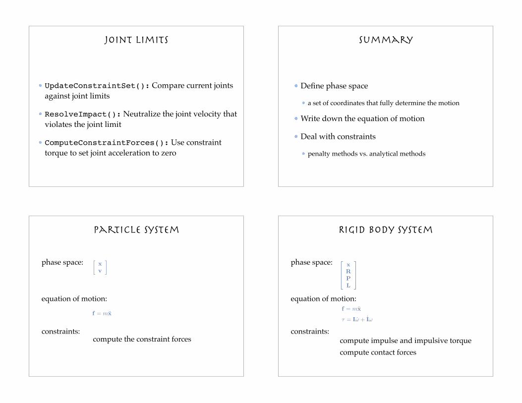
Joint limits

UpdateConstraintSet(): Compare current joints against joint limits

ResolveImpact(): Neutralize the joint velocity that violates the joint limit

ComputeConstraintForces(): Use constraint torque to set joint acceleration to zero

Summary

Define phase space

a set of coordinates that fully determine the motion

Write down the equation of motion

Deal with constraints

penalty methods vs. analytical methods

Particle system

phase space:

equation of motion:

constraints:

[

x

v

]

f = mx

compute the constraint forces

Rigid body system

phase space:

equation of motion:

constraints:

x

R

P

L

f = mx

τ = Iω + Iω

compute impulse and impulsive torque

compute contact forces

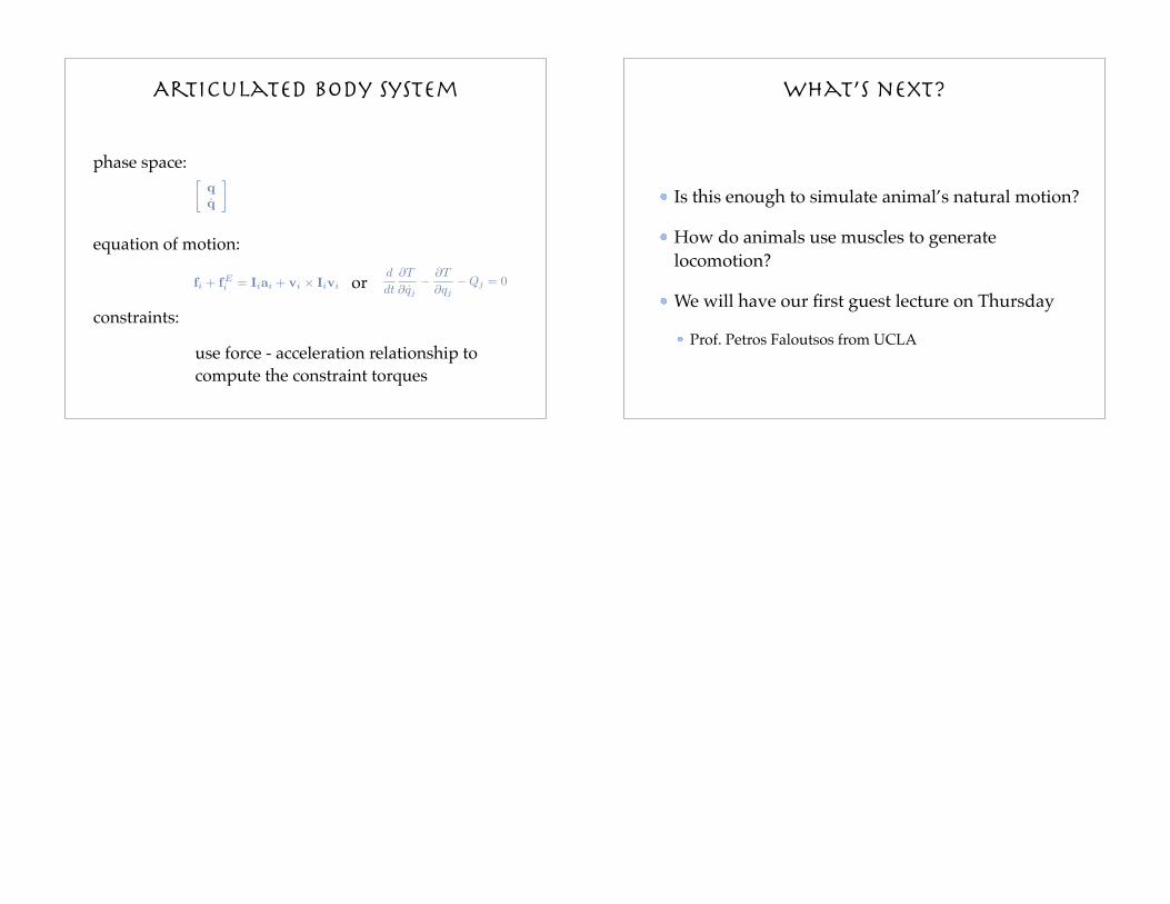
Articulated body system

phase space:

equation of motion:

constraints:

[

q

q

]

fi + fE

i = Iiai + vi × Iivi

use force - acceleration relationship to

compute the constraint torques

d

dt

∂T

∂qj

−

∂T

∂qj

− Qj = 0or

What’s next?

Is this enough to simulate animal’s natural motion?

How do animals use muscles to generate locomotion?

We will have our first guest lecture on Thursday

Prof. Petros Faloutsos from UCLA