Brigham Young University Brigham Young University

BYU ScholarsArchive BYU ScholarsArchive

Theses and Dissertations

2013-07-05

Aqueous Henry's Law Constants, Infinite Dilution Activity Aqueous Henry's Law Constants, Infinite Dilution Activity

Coefficients, and Water Solubility: Critically Evaluated Database, Coefficients, and Water Solubility: Critically Evaluated Database,

Experimental Analysis, and Prediction Methods Experimental Analysis, and Prediction Methods

Sarah Ann Brockbank Brigham Young University - Provo

Follow this and additional works at: https://scholarsarchive.byu.edu/etd

Part of the Chemical Engineering Commons

BYU ScholarsArchive Citation BYU ScholarsArchive Citation Brockbank, Sarah Ann, "Aqueous Henry's Law Constants, Infinite Dilution Activity Coefficients, and Water Solubility: Critically Evaluated Database, Experimental Analysis, and Prediction Methods" (2013). Theses and Dissertations. 3691. https://scholarsarchive.byu.edu/etd/3691

This Dissertation is brought to you for free and open access by BYU ScholarsArchive. It has been accepted for inclusion in Theses and Dissertations by an authorized administrator of BYU ScholarsArchive. For more information, please contact scholarsarchive@byu.edu, ellen_amatangelo@byu.edu.

Aqueous Henry’s Law Constants, Infinite Dilution Activity Coefficients,

and Water Solubility: Critically Evaluated Database,

Experimental Analysis, and Prediction Methods

Sarah A. Brockbank

A dissertation submitted to the faculty of Brigham Young University

in partial fulfillment of the requirements for the degree of

Doctor of Philosophy

W. Vincent Wilding, Chair Richard L. Rowley Thomas A. Knotts Randy S. Lewis

Dean R. Wheeler

Department of Chemical Engineering

Brigham Young University

July 2013

Copyright © 2013 Sarah A. Brockbank

All Rights Reserved

ABSTRACT

Aqueous Henry’s Law Constants, Infinite Dilution Activity Coefficients, and Water Solubility: Critically Evaluated Database,

Experimental Analysis, and Prediction Methods

Sarah A. Brockbank Department of Chemical Engineering, BYU

Doctor of Philosophy

A database containing Henry’s law constants, infinite dilution activity coefficients and solubility data of industrially important chemicals in aqueous systems has been compiled. These properties are important in predicting the fate and transport of chemicals in the environment. The structure of this database is compatible with the existing DIPPR® 801 database and DIADEM interface, and the compounds included are a subset of the compounds found in the DIPPR® 801 database. Thermodynamic relationships, chemical family trends, and predicted values were carefully considered when designating recommended values.

Henry’s law constants and infinite dilution activity coefficients were measured for toluene, 1-butanol, anisole, 1,2-difluorobenzene, 4-bromotoluene, 1,2,3-trichlorobenzene, and 2,4-dichlorotoluene in water using the inert gas stripping method at ambient pressure (approximately 12.5 psia) and at temperatures between 8°C and 50°C. Fugacity ratios, required to determine infinite dilution activity coefficients for the solid solutes, were calculated from literature values for the heat of fusion and the liquid and solid heat capacities. Chemicals were chosen based on missing or conflicting data from the literature.

A first-order temperature-dependent group contribution method was developed to predict Henry’s law constants of hydrocarbons, alcohols, ketones, and formats where none of the functional groups are attached directly to a benzene ring. Efforts to expand this method to include ester and ether groups were unsuccessful. Second-order groups were developed at a reference condition of 298.15 K and 100 kPa. A second-order temperature-dependent group contribution method was then developed for hydrocarbons, ketones, esters, ethers, and alcohols. These methods were compared to existing literature prediction methods. Keywords: DIPPR, database, Henry’s law constant, water solubility, infinite dilution activity coefficient

ACKNOWLEDGEMENTS

I would like to thank my advisor, Dr. Vincent Wilding, as well as Dr. Neil Giles for

helping me troubleshoot in the lab and for providing me with feedback on presentations, reports,

and papers. I thank Dr. Richard Rowley for his helpful, detailed comments on my writing.

AIChE and DIPPR®801 are thanked for project funding. I thank Jenna Russon, Doug Nevers,

and Coleman Vaclaw for database, programming, and lab help. I thank the many DIPPR®801

programmers for all of their help programming and debugging.

I want to thank my family members for their love and support throughout this journey. I

thank my husband, Bryan Brockbank, for being willing to go to the lab with me at strange hours.

I thank his patience as I have missed birthdays and an anniversary on top of having to live in

different states for a period of time in order for me to finish this degree. I also thank Brad

Brockbank, Jennie Linford, and Quinn Linford for being willing to lend a hand in the lab at

strange hours. I thank my Purcell and Brockbank parents as well as grandparents for all of their

prayers, love, and support. Most importantly, I want to express gratitude for my Savior, Jesus

Christ, who has given me strength and understanding beyond my own abilities.

v

TABLE OF CONTENTS

LIST OF TABLES ........................................................................................................................ vii LIST OF FIGURES ....................................................................................................................... xi 1 Introduction ............................................................................................................................. 1 2 Overview of Properties ............................................................................................................ 5

2.1 Definitions and Uses ........................................................................................................ 5 2.1.1 Solubility of a Compound in Water .......................................................................... 5 2.1.2 Solubility of Water in a Compound .......................................................................... 6 2.1.3 Henry’s Law Constant .............................................................................................. 6 2.1.4 Infinite Dilution Activity Coefficients: Chemical in Water ................................... 10 2.1.5 Infinite Dilution Activity Coefficients: Water in Chemical ................................... 10 2.1.6 Octanol/Water Partition Coefficient ....................................................................... 11

2.2 Experimental Techniques ............................................................................................... 11 2.2.1 Solubilities .............................................................................................................. 11 2.2.2 Henry’s Law Constants ........................................................................................... 12 2.2.3 Infinite Dilution Activity Coefficients .................................................................... 12 2.2.4 Octanol/Water Partition Coefficients ...................................................................... 13

3 Database Overview ................................................................................................................ 15 3.1 Background .................................................................................................................... 15 3.2 Database Structure and Data Entry ................................................................................ 16 3.3 Unit Conversions ............................................................................................................ 20

4 Data Evaluation ..................................................................................................................... 23 4.1 Property Relationships ................................................................................................... 23 4.2 Experimental Factors ...................................................................................................... 30 4.3 Temperature-Dependent Evaluation .............................................................................. 32

4.3.1 Error Calculations ................................................................................................... 36 4.3.2 Critical Solution Temperatures ............................................................................... 40 4.3.3 Chemical Family Plots ............................................................................................ 43 4.3.4 Other Data Analysis Notes...................................................................................... 48

4.4 Constant Values .............................................................................................................. 48 4.4.1 Chemical Family Plot Regressions ......................................................................... 49 4.4.2 Averaging ................................................................................................................ 62

4.5 American Petroleum Institute Recommendations .......................................................... 63 4.6 Comparison with Literature Recommendations and Predicted Values .......................... 64 4.7 Summary ........................................................................................................................ 72

5 Experimental Methods........................................................................................................... 75 5.1 Materials ......................................................................................................................... 75 5.2 Inert Gas Stripping Theory ............................................................................................. 76 5.3 Apparatus and Procedure ............................................................................................... 83

6 Experimental Results and Discussion ................................................................................... 89 7 Prediction Methods .............................................................................................................. 101

7.1 Overview of Prediction Method Types ........................................................................ 101 7.2 Prediction Method Selection ........................................................................................ 103

7.2.1 Method of Sedlbauer et al. [22, 191, 283] ............................................................ 106

vi

7.2.2 Method of Plyasunov and Shock [284] ................................................................. 107 7.2.3 Methods of Lau et al. [39] ..................................................................................... 108 7.2.4 Method of Kühne, Ebert, and Schüürmann [285] ................................................. 109 7.2.5 Existing Method Comparison ............................................................................... 109

7.3 Prediction Method Development ................................................................................. 110 7.3.1 Data Selection ....................................................................................................... 113 7.3.2 Validation Techniques .......................................................................................... 114 7.3.3 First-Order Group Contribution Method .............................................................. 116 7.3.4 Second-Order Group Contribution Method .......................................................... 121 7.3.5 Method Application Summary .............................................................................. 131 7.3.6 Method Comparison and Recommendations ........................................................ 131

8 Summary.............................................................................................................................. 135 8.1 Recommendations for Future Work ............................................................................. 137

9 References ........................................................................................................................... 139 Appendix A. Experimental Method Details............................................................................ 163 Appendix B. Fugacity Error Propagation ............................................................................... 179 Appendix C. Summary of Recommended Values .................................................................. 181 Appendix D. Experimental Data ............................................................................................. 273 Appendix E. Prediction Method Sample Calculations ........................................................... 289

E.1 First-Order Group Contribution Method ...................................................................... 289 E.1.1. 1,2,4,5-Tetramethylbenzene.................................................................................. 289 E.1.2. 2,2-Dimethylhexane .............................................................................................. 290 E.1.3. Methyl ethyl ketone .............................................................................................. 290

E.2 Second-Order Group Contribution Method ................................................................. 291 E.2.1. 3-Methyl-1-butanol ............................................................................................... 291 E.2.2. Ethylbenzene ......................................................................................................... 292 E.2.3. n-Butyl ethyl ether ................................................................................................ 292

vii

LIST OF TABLES

Table 3.1: Abbreviations used in 801E database .......................................................................... 15

Table 3.2: Summary of 801E entries ............................................................................................ 17

Table 3.3: Summary of the number of evaluated compounds (#) per chemical family ................ 18

Table 3.4: Unit conversion assumptions ....................................................................................... 21

Table 4.1: Number of compounds with recommended values ..................................................... 28

Table 4.2: Summary of property relationships used in this study................................................. 28

Table 4.3: DIPPR® 801 equation numbers ................................................................................... 34

Table 4.4: Equation comparisons used in data analysis ................................................................ 34

Table 4.5: Summary of uncertainty determinations for temperature-dependent regressions ....... 37

Table 4.6: Chemical families with evaluated compounds exhibiting critical solution behavior .. 40

Table 5.1: Compounds and purities .............................................................................................. 75

Table 5.2: Constant GC conditions ............................................................................................... 85

Table 5.3: GC conditions for each compound .............................................................................. 85

Table 6.1: Toluene and 1-butanol results at ambient pressure (approximately 12.5 psia) ........... 90

Table 6.2: Flow rates tested and used in this study....................................................................... 91

Table 6.3: Maximum headspace concentrations possible in this study ........................................ 92

Table 6.4: kH and γi∞ values at ambient pressure (approximately 12.5 psia) ................................ 96

Table 7.1: kH prediction methods at 298.15 K ............................................................................ 104

Table 7.2: kH temperature-dependent prediction methods excluded from this study ................. 105

Table 7.3: kH temperature-dependent prediction methods chosen for evaluation....................... 105

Table 7.4 Temperature-dependent kH prediction method comparison for select compounds .... 111

Table 7.5: Summary of performance for first-order group contribution temperature- dependent method for hydrocarbons ........................................................................................... 116

viii

Table 7.6: Summary of performance for first-order group contribution temperature- dependent method for alcohols, ketones, and formates .............................................................. 118

Table 7.7: Summary of parameter estimates for the first-order method ..................................... 120

Table 7.8: Summary of hydrocarbon second-order group contributions for reference values at 298.15 K and 0.1 MPa ............................................................................................................ 123

Table 7.9: Performance summary of the second-order temperature-dependent group contribution method for alkylbenzenes ....................................................................................... 124

Table 7.10 Second-order alcohol groups .................................................................................... 125

Table 7.11: Summary of performance for second-order temperature-dependent group contribution method for esters, ethers, ketones, and alcohols .................................................... 128

Table 7.12: Summary of second-order temperature-dependent model values ........................... 130

Table 7.13: Second-order method correction factor ................................................................... 131

Table 7.14: Comparison of methods from this study with existing methods ............................. 133

Table A.1: xiaq experimental methods ......................................................................................... 163

Table A.2: kH experimental methods .......................................................................................... 165

Table A.3: γi∞ experimental methods .......................................................................................... 169

Table A.4: KOW experimental methods .................................................................................... 172

Table C.1: Abbreviations used in regression tables .................................................................... 181

Table C.2: kH regression summary .............................................................................................. 182

Table C.3: γi∞ regression summary ............................................................................................. 201

Table C.4: xiaq regression summary ............................................................................................ 220

Table C.5: Summary of constant value recommendations (298.15 K and 1 atm) ...................... 249

Table D.1: Abbreviations used in tables with experimental run information ............................. 273

Table D.2: Cell data for each experimental run .......................................................................... 274

Table D.3: Experimental run information—additional parameters ............................................ 279

ix

Table D.4: Experimental run calculated values .......................................................................... 284

xi

LIST OF FIGURES

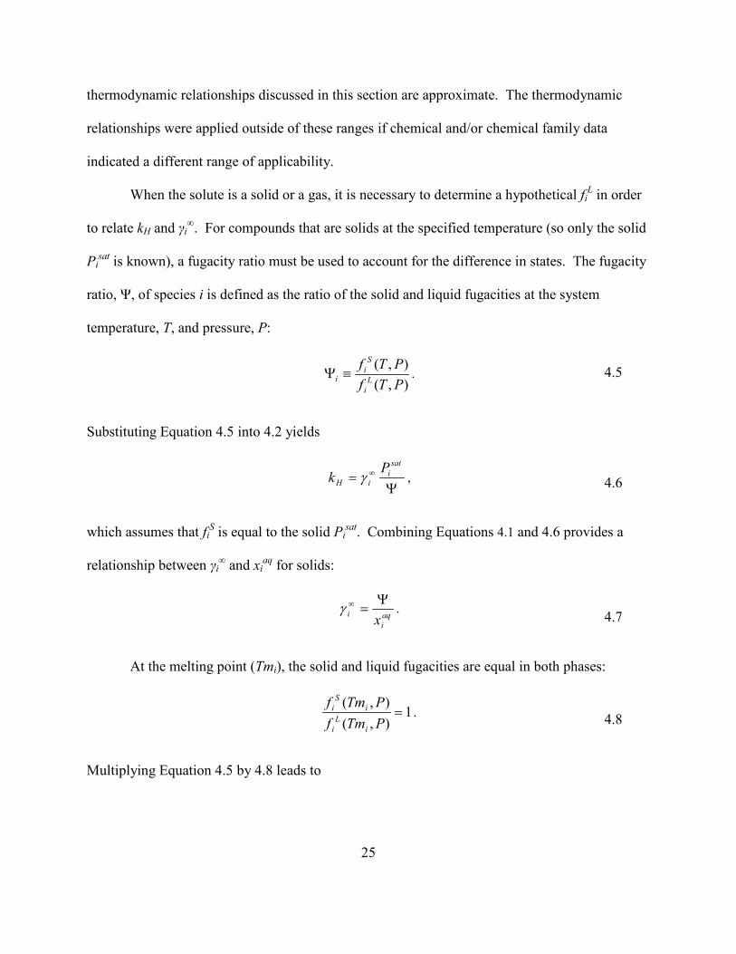
Figure 4.1: 2-Methyl-1-butanol kH, xiaq, and γi

∞ data plotted as ln(kH) versus inverse temperature. References: [44-48] .................................................................................................. 29

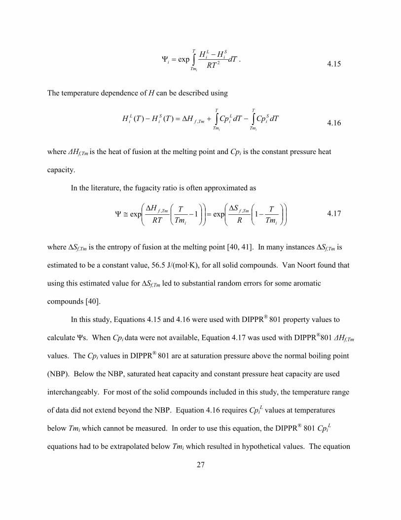
Figure 4.2: 2-Methyl-1-butanol kH, xiaq, and γi

∞ data plotted as ln(xiaq) versus inverse

temperature References: [44-48] ................................................................................................... 30

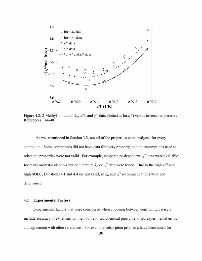
Figure 4.3: Literature xiaq data for vanillin. References: a [50], b [51], c [52], d [53], e [54] ...... 31

Figure 4.4: Uncertainty determination of experimental datasets .................................................. 39

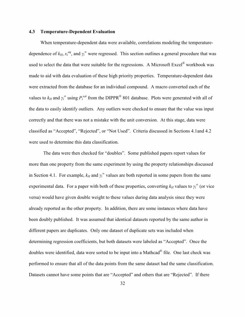
Figure 4.5: 2-Butanol ln(xiaq) data and regression. References: [55-62] ...................................... 41

Figure 4.6: ln(xiaq) data and regression for p-chlorophenol. References: [63-67] ........................ 42

Figure 4.7: Residual plot from p-chlorophenol ln(xiaq) regression ............................................... 42

Figure 4.8: n-Alcohol ln(xiaq) regressions based on experimental data versus inverse

temperature. Initial C8 regression based on experimental data (C8) and updated C8 regression based on experimental data and predicted values from the family plot (C8- Exp&Pred) are both shown. .......................................................................................................... 44

Figure 4.9: 1-Heptanol values plotted as ln(kH) versus inverse temperature. 1-Octanol (C8) and 1-hexanol (C6) regressions obtained from experimental data shown along with the average of these two regressions (Avg C6 & C8). References: a [47], b [69], c [68] (*reference reports values using two different experimental methods), d [70], e [71], xi

aq data [44, 72-80] ............................................................................................................................. 45

Figure 4.10: n-Alcohol ln(γi∞) regressions based on experimental data versus inverse

temperature ................................................................................................................................... 47

Figure 4.11: n-Alcohol ln(kH) regressions based on experimental data versus inverse temperature ................................................................................................................................... 47

Figure 4.12: 1-Alkene kH and xiaq data at 298.15 K plotted as ln(xi

aq) versus carbon number (#C). References: [47, 72, 84-87] ................................................................................................. 51

Figure 4.13: 1-Alkene ln(kH) values at 298.15 K from this study (“Smoothed” and “Predicted”) and HENRYWIN bond-contribution prediction method [83] plotted as a function of carbon number (#C) ................................................................................................... 51

Figure 4.14: 1-Iodoalkane ln(kH) values at 298.15 K from temperature-dependent regressions (Temp. Dep. Smoothed), constant value family plot (Const. Val. Smoothed), the literature (data) [47], and HENRYWIN bond-contribution method [83] plotted as a function of carbon number (#C) ................................................................................................... 52

xii

Figure 4.15: n-Alcohol “Smoothed” values from temperature-dependent evaluations and literature values plotted as ln(xi

aq) versus carbon number (#C). Solid symbols represent values at 298.15 K. Other values are at temperatures ranging from 277.15 K to 307.15 K. References: a [70], b [91], c [88], d [90], e [92], f [89], g [93] .................................................... 53

Figure 4.16: n-Alkane “Smoothed” values from temperature-dependent evaluations and literature (Data) xi

aq values at 298.15 K. References: [85, 95-104] ............................................. 55

Figure 4.17: n-Alkylbenzene ln(xiaq) values at 298.15 K from temperature-dependent

regressions (Temp. Dep. Smoothed), constant value family plot (Const. Val. Smoothed), and the literature (Data) plotted as a function of carbon number (#C). References: [105, 106] .. 55

Figure 4.18: di-n-Alkyl phthalate ln(xiaq) values at 298.15 K from temperature-dependent

regressions (Temp. Dep. Smoothed), constant value family plot (Const. Val. Smoothed), and the literature (Data and Rejected Data) plotted as a function of the number of carbons on the alkyl chains (#C). References: [107-115] .......................................................................... 56

Figure 4.19: di-n-Alkyl phthalate “Smoothed” ln(kH) values at 298.15 K from this study and from HENRYWIN[83] bond-contribution method ................................................................ 57

Figure 4.20: Literature data of diethyl phthalate at 298.15 K plotted as ln(kH) compared with HENRYWIN bond-contribution value and reported experimental value [83]. References: a [111], b [116], c [109], d [112], e [110], f [107] .................................................... 58

Figure 4.21: Smoothed ln(xiaq) and ln(Pi

sat) [117] of di-n-alkyl phthalates at 298.15 K .............. 59

Figure 4.22: Cycloalkane and cycloalkene ln(xiaq) and ln(Pi

sat) values at 298.15 K plotted as a function of carbon number (#C). References: [86, 117] ............................................................ 61

Figure 4.23: Cycloalkane and cycloalkene ln(kH) values at 298.15 K compared to HENRYWIN bond-contribution values [83] ................................................................................ 61

Figure 4.24: Triethylamine xiaq, γi

∞, and kH literature data. References: [118-127] ..................... 62

Figure 4.25: Methanol γi∞ regressions from this study and Dohnal et al. [21]. References:

[45, 48, 69, 70, 77, 167-182]......................................................................................................... 66

Figure 4.26: n-Propyl formate xiaq data, regression from this study, and IUPAC-NIST [159]

regression compared to ethyl formate xiaq data. References: [183, 184] ...................................... 67

Figure 4.27: di-n-Propyl ether xiaq regressions from this study and from IUPAC-NIST [158].

References: [47, 172, 186-189] ..................................................................................................... 68

Figure 4.28: 3-Methyl-3-pentanol xiaq regressions from this study and from IUPAC-NIST

[150]. References: [44, 190] ......................................................................................................... 69

xiii

Figure 4.29: Cumene xiaq data compared with Sedlbauer et. al [191] predicted values and

API [128] and IUPAC-NIST [136] recommendations. References: a [194], b [192], c [193], d [105] ........................................................................................................................................... 71

Figure 4.30: 2,2,5-Trimethylhexane xiaq data plotted as ln(kH) compared with Sedlbauer et.

al [191] predicted values. References: a [195], b [86] ................................................................. 72

Figure 5.1: Inlets and outlets of saturation and stripping cells used in mass balances ................. 78

Figure 5.2: IGS apparatus ............................................................................................................. 85

Figure 6.1: GC data for two separate 1,2-difluorobenzene experiments at 323.15 K and a N2 flow rate of 40 mL/min that resulted in different slopes (a) ......................................................... 94

Figure 6.2: Cumulative slopes (a) from GC data shown in Figure 6.1 as a function of time ....... 94

Figure 6.3: 1,2,3-Trichlorobenzene kH values from this study and from literature. Values from references marked with an asterisk (*) are xi

aq data converted to kH values using Equation 4.1. References: a [209], b [71], c [206], d* [210], e* [211], f* [212], g* [213], h* [205], i* [207] , j* [214] .......................................................................................................... 97

Figure 6.4: Anisole kH values from this study and from the literature. Values from references marked with an asterisk (*) are xi

aq data converted to kH values using Equation 4.1. References: a [172], b [206], c* [215], d* [118], e* [216] ................................................... 98

Figure 6.5: 2,4-Dichlorotoluene kH values from this study and from the literature. Values from xi

aq data were converted to kH values using Equation 4.1. Reference: [8] .......................... 99

Figure 6.6: 1,2-Difluorobenzene kH values from this study and from the literature. Values from xi

aq data were converted to kH values using Equation 4.1. Reference: [207] ...................... 99

Figure 6.7: 4-Bromotoluene kH values from this study and from the literature. Values from xi

aq data were converted to kH values using Equation 4.1. References: [47, 208] ..................... 100

Figure 7.1: Plot of experimental versus model values for the first-order temperature- dependent group contribution method for hydrocarbons ............................................................ 117

Figure 7.2: Plot of experimental versus model values for the first-order temperature- dependent group contribution method for alcohols, ketones, and formates ............................... 119

Figure 7.3: Plot of experimental versus model values for the second-order temperature- dependent group contribution method for alkylbenzenes and alkanes ....................................... 125

Figure 7.4: Initial second-order group contribution model performance for functional groups .......................................................................................................................................... 126

xiv

Figure 7.5: Corrected second-order group contribution model performance for functional groups .......................................................................................................................................... 128

Figure 7.6: Plot of experimental versus model values for the second-order temperature- dependent group contribution method for esters, ethers, ketones, and alcohols......................... 129

1

1 Introduction

A growing global concern is the fate and transport of chemicals in the environment in

addition to health and safety risks associated with chemical exposure. The Toxic Substances

Control Act (TSCA) was passed in 1976 in the United States, and it requires the U.S.

Environmental Protection Agency (EPA) to estimate risks of chemicals prior to

commercialization [1]. The EPA has developed a process to estimate risks associated with a

chemical to ensure it will not pose an unreasonable risk if commercialized. Properties used in

these risk assessments include water solubility, octanol/water partition coefficients, and Henry’s

law constants. The Registration, Evaluation and Authorization of Chemicals (REACH) is a new

policy concerning chemical regulations in Europe that became effective June 2007 throughout

the European Union [2]. REACH requires industry to provide health, safety, and environmental

information that will aid in the management of risks. Properties required by REACH include

water solubility and the octanol/water partition coefficient [3, 4].

It is estimated that experimental values are available for less than 1% of the

approximately 84,000 compounds included in TSCA and the 100,000 compounds included in

REACH [5]. This means that environmental regulations rely heavily on prediction methods. A

prediction method is only as good as the data used to develop the method. Prediction methods

developed using evaluated data allow for superior prediction method development performance.

2

DIPPR® Projects 911 and 912 were initiated in 1991 by AIChE/DIPPR® with the goal of

compiling data and prediction methods for important environmental, safety, and health properties

of chemicals that are regulated and important in industry [6]. The information was compiled as

the Environmental and Safety Properties (ESP) database. In November 2009, the DIPPR® 801

steering committee decided that a thorough review should be conducted on select compounds in

order to evaluate the status of the DIPPR® ESP database. As a result of the review, it was

decided to build a new database (801E) focusing on select properties. The properties of primary

interest are aqueous Henry’s law constant (kH), infinite dilution activity coefficient of a chemical

in water (γi∞), and the solubility of a compound in water (xi

aq). The infinite dilution activity

coefficient of water in the chemical, the solubility of water in a chemical, and the octanol/water

partition coefficients were included when available. However, these properties were given low

priority meaning they were not reviewed as thoroughly due to time constraints and lower interest

from the DIPPR® steering committee. An overview of the properties included in the 801E

database is given in Chapter 2.

The first objective of this project was to compile a database containing primary,

experimental data for kH, γi∞, and xi

aq for 500 compounds. An overview of the database is given

in Chapter 3. Accepted values were designated for kH, γi∞, and xi

aq by evaluating the available

literature data. Recommendations were given for values at a single temperature or over a

temperature range depending on the amount of available literature data. The data evaluation

process is described in Chapter 4. The second objective was to perform temperature-dependent

measurements of kH and γi∞ for seven compounds to fill in data gaps and provide clarification for

inconsistencies with reported experimental values. The experimental methods and results are

3

given in Chapters 5 and 6. The third objective was to analyze and refine kH prediction methods

using the evaluated database which is described in Chapter 7.

5

2 Overview of Properties

2.1 Definitions and Uses

2.1.1 Solubility of a Compound in Water

Water solubility (xiaq) is the maximum amount of a substance (gas, liquid, or solid) that

will dissolve in a specified amount of water at a defined temperature and pressure [1]. This is an

important property for predicting a chemical’s environmental fate and its effects on biological

systems. Highly water-soluble chemicals absorb easily into biological systems and typically

degrade readily in the environment. However, highly water-soluble chemicals do not easily

adsorb on soils and sediments or bioaccumulate. Solubility is a function of temperature, but it is

often treated as a constant over environmental temperature ranges [7]. Generally, solubility

increases with increasing temperature [8]. Other factors that affect solubility include pressure,

pH, and the presence of additional chemical species [9-11]. In this project, the focus is xiaq data

of a single solute in pure water measured at temperatures below 373 K at or near atmospheric

pressure. However, high-temperature data have been included for some compounds.

Some systems exhibit upper and/or lower critical solution temperatures. At temperatures

below or above the lower or upper critical solution temperatures, respectively, the compound and

water are completely soluble in each other resulting in one liquid phase. Compounds that have

6

critical solution temperatures within the temperature limits of this study are noted in the

database. In some studies reporting solubility data for solid compounds, compositions are

reported for multiple portions of the phase diagrams (i.e. ice compositions). These other phase

data are input (or mentioned) in the database. However, only data that meet the definition above

of xiaq for liquid water were analyzed in this study.

2.1.2 Solubility of Water in a Compound

The solubility of water in a compound is defined as the maximum amount of water that

will dissolve in a given amount of compound at a specified temperature and pressure. This

property is often measured in conjunction with xiaq (xi

aq and the solubility of water in a

compound are reported as mutual solubility values). Recommended values were not provided in

this study because this is a low priority property, so a thorough literature review was not

conducted for this property. This property is not as important as other properties when

determining the environmental fate of hydrophobic compounds. However, data were briefly

examined during the data analysis portion of this project. This is discussed in more detail in

Section 4.1.

2.1.3 Henry’s Law Constant

In environmental impact studies, Henry’s law constants (kHs) are used to determine the

fate and transport of chemicals in air and water by determining volatilization or absorption

tendencies [12, 13]. Chemicals with higher kHs partition towards air while chemicals with lower

kHs partition towards water [1]. Additional uses of kH values include the design and optimization

7

of air-stripping columns that remove contaminants from groundwater as well as applications in

the pharmaceutical and food science industries [14].

The definition of kH is given by

i

Li

xH xf

ki

ˆlim

0→≡ , 2.1

where Lif̂ is the partial fugacity of compound i in solution, and xi is the mole fraction in the

liquid phase [15-17]. This definition is applicable at all temperatures and pressures [16].

Application of l’Hôpital’s rule equates kH to the slope of the tangent line of the Lif̂ versus xi

curve at xi = 0. The equation of this tangent line produces Henry’s law:

HiL

i kxf =ˆ . 2.2

Most systems are represented by Henry’s law for small values of xi. The concentration at which

system behavior deviates from Henry’s law varies with every system, although an upper

concentration of 0.01 mole fraction has been recommended [18, 19]. An activity coefficient can

be added to correct for non-idealities caused by higher concentrations. Corrections can also be

introduced for systems at high pressures. If ideal gas behavior is assumed, Equation 2.2

simplifies to

Hii kxPy = , 2.3

where yi is the mole fraction in the vapor phase and P is the total pressure. In this study, kH

refers to aqueous systems.

8

The Gibbs energy of hydration, ∞∆ hydG , is defined as the process of transferring a

molecule from an ideal gas at a reference pressure to a hypothetical infinitely dilute solution with

a solute mole fraction of unity[20-22]. A relationship between kH and ∞∆ hydG is

∞∆=

hyd

ref

H GPkRT ln , 2.4

where Pref is 100 kPa. Unit conversions may need to be included in Equation 2.4 depending on

the units of the reference state. Temperature and pressure derivatives link ∞∆ hydG to additional

properties often referred to as derivative properties. These derivative properties are the enthalpy

of hydration ( ∞∆ hydH ), heat capacity of hydration ( ∞∆ hydCp ), and partial molar volume ( ∞V ) at

infinite dilution:

∞∆−=

∂∂

hydP

H HTkRT ln2 , 2.5

∞∆−=

∂∂

∂∂

hydP

H CpTkRT

Tln2 , 2.6

∞=

∂∂ V

PkRT

T

Hln. 2.7

Data for derivative properties were not included in this study. These relationships are mentioned

because they are used in some prediction methods (discussed in Chapter 7).

Values of kH first increase with temperature, reach a maximum typically between 373 and

473 K, and then decrease with temperature [22]. Most compounds do not have enough reported

temperature-dependent data to see this whole trend. There are several different reported units for

9

kH. Units include the ratio of partial pressure (Pi) and solute concentration in a dilute solution,

Pi/xi or Pi/CiL, where Ci

L is the concentration, in units such as moles per liter, in the liquid phase.

The aqueous kH is also reported as a ratio of the air and water concentrations making it unitless—

either yi/xi or Ciair/Ci

L where Ciair is the concentration in the vapor phase. While both of these

ratios are unitless, their numerical values can differ significantly [23]. A universal conversion

between the various ratios is done assuming the vapor phase behaves as an ideal gas and that the

solution is pure water. These assumptions are valid under environmental conditions.

The air-water partition coefficient is the mole fraction ratio of the solute in air to that in

water, and by definition it is not limited by the requirement of infinite dilution. In the

environmental field, it is often used synonymously with kH despite different thermodynamic

definitions [17, 24-26]. The conversion between the air-water partition coefficient and kH is

straightforward for dilute solutions at environmental conditions which is why the terms are often

used synonymously. The conversion becomes more complex at high temperatures and pressures.

In the database, any reported kHs or air-water partition coefficients that are measured for

environmental purposes were treated as experimental kHs.

The kH values measured for compounds that hydrate or dissociate in water are typically

apparent kH values. Hydration or dissociation can be accounted for in order to calculate an

intrinsic kH [23, 27]. No efforts were made to account for dissociation or hydration in this study.

It is assumed that literature kH values are apparent kH values unless otherwise noted. In this

study, kH data for strong electrolytes were typically left unevaluated due to the spread in data

partially caused by the variety of pH conditions reported in the literature.

10

2.1.4 Infinite Dilution Activity Coefficients: Chemical in Water

Activity coefficients are an indicator of the nonideal behavior of a mixture. The activity

coefficient of species i (γi) is defined as

Lii

ii fx

f̂≡γ 2.8

where if̂ is the partial fugacity of compound i in solution, Lif is the pure liquid fugacity of

species i, and xi is the mole fraction in the liquid phase. The infinite dilution activity coefficient

(γi∞) is the limiting value as xi goes to zero. In this discussion, γi

∞ specifically refers to systems

in which the solvent is water.

Thermodynamic relationships exist between γi∞ and xi

aq, kH and the octanol-water

partition coefficient [28]. Relationships between γi∞, xi

aq, and kH are given in Section 4.1.

Environmental applications of γi∞s include assessments of aquatic toxicity, leaching, soil and

sediment transport properties, sorption, bioconcentration, and volatilization [29]. Other

applications include modeling evaporation rates [12], choosing the most selective solvent for

extraction [30], and developing constants in empirical equations for excess functions which are

then used to predict fluid phase equilibrium.

2.1.5 Infinite Dilution Activity Coefficients: Water in Chemical

The discussion for γi∞ applies here for the infinite dilution activity coefficient of water in

a chemical, but the difference is that water is the solute and the chemical is the solvent. This

property has low priority in this study because it is uncommon in environmental applications.

Thorough literature and data analysis reviews have not been conducted in this study.

11

2.1.6 Octanol/Water Partition Coefficient

The octanol/water partition coefficient (KOW) is the equilibrium ratio of the

concentrations of a chemical substance in n-octanol to that in water [1]. It is dimensionless and

is often expressed as the base 10 logarithm. It can be used to predict the distribution of a

chemical in living organisms (because octanol has a similar carbon to oxygen ratio as is found in

lipid materials in animals [31]) or in the environment. For almost all non-ionic organic

substances, KOW can be used to estimate other properties such as xiaq, soil/sediment absorption,

biological absorption, bioaccumulation, and toxicity [1]. This property is temperature dependent

[32]. KOW is a low priority property in this study since there are existing databases of KOW

values [33, 34]. Data have been input when included in articles containing high priority

properties. However, thorough literature and data analysis reviews have not been conducted.

2.2 Experimental Techniques

There are a variety of experimental methods that have been reported to measure the

properties included in this study. Many of the methods can be used to obtain more than one

property due to the relationships between properties (discussed in Section 4.1).

2.2.1 Solubilities

The methods to measure solubilities in which the solvent is a liquid are similar for all

solute-solvent combinations. The solubility of water in a compound and xiaq are often measured

in the same study and reported as mutual solubility data. Many solubility methods consist of

equilibrating water with excess compound and analyzing the composition of one or both of the

resulting phases. There are a variety of equilibration and analytical techniques employed in the

12

literature to accomplish this. The experimental methods are applicable over limited solubility

ranges due to adsorption and emulsion problems and detection limitations, so the solubility needs

to be predicted in order to choose the correct testing method. The methods are discussed in

further detail in Appendix A.

2.2.2 Henry’s Law Constants

Static or dynamic equilibration techniques can be used to measure kH. Static

equilibration involves the direct measurement of the air and/or water concentrations in a closed,

equilibrated system. Methods include single equilibration, multiple equilibration, equilibrium

partitioning in closed systems (EPICS), and variable headspace techniques. Static equilibration

techniques are usually only done for higher concentrations due to the difficulty in measuring low

concentrations in both phases [19]. Dynamic equilibration involves some type of air/water

exchange. Two methods of this type are inert gas stripping and concurrent flow. Experimental

methods are discussed in more detail along with limitations in Appendix A.

2.2.3 Infinite Dilution Activity Coefficients

There is overlap between the methods used to measure kH and γi∞ due to the

thermodynamic relationship between these two properties (see Section 4.1). Many papers report

both properties from the same experimental data. Often multiple techniques are required to

measure values over a range of temperatures due to measurement limitations. It is ideal to apply

more than one measurement technique to ensure consistency in results [35]. Experimental

methods are discussed in more detail along with limitations in Appendix A.

13

2.2.4 Octanol/Water Partition Coefficients

The methods used to measure KOWs are similar to some of the methods used to measure

xiaq. These methods include equilibrating a compound with 1-octanol and water and determining

the concentration using an analytical technique. Another common method involves estimating

the KOW based on gas chromatography (GC) retention data of the compound and reference

compounds. Each method covers a range of values, so KOW should be predicted in order to

determine the proper testing technique. Experimental methods are discussed in more detail along

with limitations in Appendix A.

15

3 Database Overview

3.1 Background

It was decided at the May 2010 DIPPR® meeting by BYU staff and DIPPR® sponsors to

build a new database containing the properties outlined in Chapter 2 because more work would

be involved in fixing the ESP database than in starting fresh. In the original ESP database, data

for the properties outlined in Chapter 2 were only included at 298.15 K, and the properties were

included in the constant values tables. It was decided to include temperature-dependent data in

addition to the constant values (defined at 298.15 K) in the new database. Due to the notation

allowed in Microsoft Access®, the properties had to be represented by letter abbreviations instead

of symbols. Separate abbreviations were required for the constant value and temperature-

dependent properties. The abbreviations are given in Table 3.1. The symbols kH, xiaq, and γi

∞

will continue to be used throughout this document in the text and plots because they are more

intuitive.

Table 3.1: Abbreviations used in 801E database

Property Constant Value Temperature-Dependent Infinite dilution activity coefficient of compound in water ACCW ACCWT Infinite dilution activity coefficient of water in compound ACWC ACWCT

Aqueous Henry’s law constant HLC HLCT Octanol/water partition coefficient KOW KOWT Solubility of compound in water SOLC SOLCT

Solubility of water in a compound SOLW SOLWT

16

3.2 Database Structure and Data Entry

This new database, DIPPR® 801E, has a similar format to the 801 database so that it is

compatible with DIADEM, the DIPPR® 801 software interface. In order to make the process of

data entry easier while reducing the opportunities for entry error, DIADEM was modified

slightly. Units were added so that they can be selected from dropdown menus. Due to

assumptions in the unit conversions, two columns were added to the database so that it stores the

original values and units in the database after the data for each property are converted to the

default unit. There is not a way to view these original values or perform more complex unit

conversions using DIADEM, but a future user of the database could look up the original value

and perform a more exact unit conversion if desired.

Data were considered constant values or temperature-dependent. The constant values

properties are defined at 298.15 K and 1 atm. Experimental values within ±5 degrees of 298.15

K were included in the constant values table. The actual temperature and pressure were included

in a note if they differed from 298.15 K or 1 atm, respectively. All values at 298.15 K were also

input as temperature-dependent data in addition to data at other temperatures. There were

instances when articles included measurements for some chemicals only at temperatures outside

of the constant value range. In these instances, the data were only entered in the temperature-

dependent table. If data of non-dissociating compounds were reported as a function of pH, only

the values at pH ≈ 7 were analyzed. When data were input, they were labeled as “Unevaluated”.

As datasets were evaluated, the label was changed to “Accepted”, “Not Used”, or “Rejected”

based on the quality of the dataset. These categories allow a future user to know which data

were considered during the evaluation process.

17

At the conclusion of this project, recommended (“Accepted”) values have been

determined for at least one property for 509 compounds. There are entries for over 800

compounds due to the data entry process; however, not all of the data have been evaluated. Data

were entered by reference, and all data for any DIPPR® 801 chemical mentioned in a reference

were included. Table 3.2 summarizes the number of data points that have been considered

during evaluation and the number of compounds with recommended values for each property.

Due to the lack of reliable data, not all of the high priority properties were analyzed for each

compound which is why each property has a different number of compounds with

recommendations. Based on the availability of temperature-dependent data, some compounds

have recommendations for a temperature range while other compounds only have

recommendations for a single temperature (typically 298.15 K). Table 3.3 summarizes the total

number of evaluated compounds per chemical family. The entry numbers given in Table 3.2

reflect the actual entries retrieved directly from the literature. They do not include the derived

entries that were added during the data evaluation process of this study (i.e. kH values derived

from xiaq data, etc.). The compound totals include the American Petroleum Institute (API)

recommendations that were accepted in this study (discussed in Section 4.5). The data

evaluation process is discussed in detail in Chapter 4.

Table 3.2: Summary of 801E entries

Property Evaluated Data Points

Compounds with Recommendations

γi∞ 1350 407

kH 3950 445 xi

aq 7617 481 Overall 12917 509

18

Table 3.3: Summary of the number of evaluated compounds (#) per chemical family

Family # Family # Family # 1-Alkenes 14 Dialkenes 2 Other Alkanes 2

2,3,4-Alkenes 4 Dicarboxylic Acids 3 Other Alkylbenzenes 10 Acetates 17 Dimethylalkanes 7 Other Amines, Imines 7

Aldehydes 19 Diphenyl/Polyaromatics 1 Other Condensed Rings 11 Aliphatic Ethers 13 Elements 6 Other Ethers/Diethers 7

Alkylcyclohexanes 4 Epoxides 6 Other Inorganics 1 Alkylcyclopentanes 1 Formates 7 Other Monoaromatics 1

Alkynes 8 Inorganic Bases 1 Other Polyfunctional C, H, O 6

Aromatic Alcohols 14 Inorganic Gases 5 Other Polyfunctional Organics 2

Aromatic Amines 16 Ketones 26 Other Saturated Aliphatic Esters 6

Aromatic Carboxylic Acids 4 Mercaptans 5 Peroxides 2

Aromatic Chlorides 11 Methylalkanes 8 Polyfunctional Acids 1

Aromatic Esters 9 Methylalkenes 2 Polyfunctional Amides/Amines 7

C, H, Br Compounds 14 n-Alcohols 18 Polyfunctional C, H, N, Halide, (O) 2

C, H, F Compounds 8 n-Aliphatic Primary Amines 8 Polyfunctional C, H, O,

Halide 6

C, H, I Compounds 7 n-Alkanes 14 Polyfunctional C, H, O, N 3 C, H, Multihalogen

Compounds 3 n-Alkylbenzenes 11 Polyfunctional C, H, O, S 1

C, H, NO2 Compounds 17 Naphthalenes 4 Polyfunctional Esters 4 C1/C2 Aliphatic

Chlorides 19 Nitriles 12 Polyols 3

C3 & Higher Aliphatic Chlorides 11 Nitroamines 3 Propionates and Butyrates 13

Cycloaliphatic Alcohols 1 Organic Salts 2 Sulfides/Thiophenes 6

Cycloalkanes 5 Other Aliphatic Alcohols 21 Unsaturated Aliphatic Esters 4

Cycloalkenes 4 Other Aliphatic Amines 9

Data were entered with the original values and units to avoid any errors from external

conversions. The only exceptions were when articles only report data as plots or regressions of

experimental values. DataThief [36] was used to extract values from plots of experimental data.

When authors only reported temperature-dependent correlations of their experimental data, the

19

correlations were used to calculate values at the measurement temperatures reported by the

authors. These values were classified as “Smoothed” in the database. Some authors report

multiple values at the same temperature. The average of these values was input in order to not

give extra weight to the dataset during analysis.

The focus of this database was on primary, experimental data. Due to time constraints,

an additional focus was on post 1950 English references. It was assumed that more recent data

are generally of higher quality than older data due to improvements in analytical techniques and

higher material purities. Many of the older and/or foreign articles were not readily available, and

the foreign articles required translating. Due to time constraints, it was not realistic for all of

these types of articles to be included. Data from these articles were selectively input based on

the availability of data from more recent English references. Data found in handbooks would be

interesting to include in the database to compare with primary data, but these references were

also excluded due to ambiguities and the time required for data entry. The original sources of

handbook data (experimental versus predicted) are often excluded or unclear making it difficult

to determine the reliability of the reported values.

Guidelines were developed that aided in data classification. These guidelines explain

how to label data (i.e., classifying data as “experimental” or “predicted”). Issues that were

encountered during the data entry process were clarified to establish consistency in the database.

The guidelines also include assumptions and limitations for the various measurement techniques

which was useful during the data analysis process.

20

3.3 Unit Conversions

In order to compare values from different references, all literature values needed to be

converted to the same units. The unit conversions for the temperature-dependent properties

accounted for the temperature-dependence of the conversion. For example, some xiaq and kH

conversions required liquid densities. When the temperature-dependent data were converted, the

liquid densities at the correct temperature were used. There were additional assumptions with

some of the unit conversions. These assumptions in addition to the default units are listed in

Table 3.4. The assumptions for the kH unit conversions are valid since the data included in the

database were typically measured at atmospheric pressure using dilute solutions. Many of the

solubility data were reported in units that did not require any assumptions in order to perform the

conversion to the default unit. When assumptions were required, it was assumed that volumes

were additive. This assumption was generally only needed for compounds with small

solubilities. Any volume changes due to non-ideality would be negligible. Initially only liquid

or theoretical liquid densities were used for the solubility conversions. In some cases

extrapolating the liquid density curve to temperatures where the compound is a solid led to

obviously erroneous values (gave negative solubility values). Therefore, the volume of the

liquid or solid solute was calculated using the liquid or solid densities, respectively, when using

additive volumes for solubility conversions. If the solute was a gas, it was assumed that the

added volume was negligible.

21

Table 3.4: Unit conversion assumptions

Property Unit Conversion Assumptions Default Units HLC • Ideal gas with pressure of 1 atm

• Solution treated as pure water (since infinitely dilute) kPa·mol/mol

SOLW/SOLC • Additive volumes if solute is a solid or liquid • Solution considered pure solvent if solute is gas • Solution considered pure solvent if solute is a solid that

does not have a solid density equation (i.e. 1-heptadecanol) • Conversions treated as per amount of solution (i.e. g/100g

solution) unless authors state otherwise (i.e. g/100g H2O)

mol frac.

ACCW/ACWC None unitless KOW None Log KOW

23

4 Data Evaluation

Because of the thermodynamic relationships between kH, xiaq, and γi

∞, reported values of

these different properties can be conveniently compared. In this study, the combined data from

the three properties were often used to obtain temperature regressions and recommended values

for each property. For compounds where the assumptions of the thermodynamic relationships

were not met (meaning the data from all the properties could not be combined), these

relationships still helped identify outliers in reported data making it easier to designate

recommended values. Notes in the database indicate the data that were combined to obtain

regressions for each compound and property. In addition, experimental factors, temperature-

dependent trends, chemical family plots, and literature recommendations were also used to

evaluate data. All of these are discussed in further detail.

4.1 Property Relationships

A relationship between kH and xiaq is given by evaluating equation 2.3 at the solubility limit

aqi

sati

H xPk =

4.1

where Pisat is the vapor pressure of solute i. This relationship is valid for hydrophobic chemicals

with xiaq values below approximately 0.001 mole fraction. It assumes that the solubility of water

24

in the compound (SOLC) is negligible so that the partial vapor pressure of solute is unaffected by

the presence of water allowing it to be treated as Pisat [12, 19, 23]. The assumptions break down

when SOLC exceeds approximately 0.1 mole fraction. In addition, xiaq and Pi

sat must reference

the same physical state [37]. In this study, a pressure of 101.325 kPa was assumed for gases in

order to convert kH to xiaq values and vice versa. For gases, kH and xi

aq are used interchangeably.

In the literature, kH values calculated from Equation 4.1 are usually reported as experimental.

A relationship between kH and γi∞ is obtained by substituting the definition of γi (Equation

2.8) into that of kH (Equation 2.1),

LiiH fk ∞= γ , 4.2

where fiL is the fugacity of pure species i in the liquid phase, and xi is the mole fraction in the

liquid phase. At atmospheric conditions for liquid solutes, this simplifies to:

satiiH Pk ∞= γ . 4.3

This relationship is more thermodynamically rigorous than Equation 4.1. Combining Equations

4.1 and 4.3 yields a relationship between γi∞ and xi

aq for hydrophobic liquids:

aqi

i x1

=∞γ . 4.4

The same assumptions that make Equation 4.1 valid also apply for Equation 4.4. Equation 4.4 is

valid for γi∞ values greater than 1000 [38]. When available, SOLC data were examined during

the data analysis procedure to check the validity of Equations 4.1 and 4.4. It is possible to use

both SOLC and xiaq to obtain γi

∞ when the assumptions of Equation 4.4 are violated [23, 39] .

However, since SOLC data were not critically evaluated, γi∞ and kH values were not determined

from xiaq when SOLC was above approximately 0.1 mole fraction. All of the valid ranges of the

25

thermodynamic relationships discussed in this section are approximate. The thermodynamic

relationships were applied outside of these ranges if chemical and/or chemical family data

indicated a different range of applicability.

When the solute is a solid or a gas, it is necessary to determine a hypothetical fiL in order

to relate kH and γi∞. For compounds that are solids at the specified temperature (so only the solid

Pisat is known), a fugacity ratio must be used to account for the difference in states. The fugacity

ratio, Ψ, of species i is defined as the ratio of the solid and liquid fugacities at the system

temperature, T, and pressure, P:

),(),(

PTfPTf

Li

Si

i ≡Ψ . 4.5

Substituting Equation 4.5 into 4.2 yields

Ψ

= ∞sat

iiH

Pk γ , 4.6

which assumes that fiS is equal to the solid Pi

sat. Combining Equations 4.1 and 4.6 provides a

relationship between γi∞ and xi

aq for solids:

aqi

i xΨ

=∞γ . 4.7

At the melting point (Tmi), the solid and liquid fugacities are equal in both phases:

1),(),(=

PTmfPTmf

iL

i

iS

i . 4.8

Multiplying Equation 4.5 by 4.8 leads to

26

),(),(

),(),(

PTfPTmf

PTmfPTf

Li

iL

i

iS

i

Si

i =Ψ . 4.9

The residual Gibbs energy, GiR, is related to f and P by

=Pf

RTG iRi ln . 4.10

Rearranging Equation 4.10 and using partial derivatives leads to

2

)ln(RTH

T

RTG

Tf R

i

P

Ri

P

i −=

∂

∂

=

∂

∂ 4.11

where HiR is the residual enthalpy. To integrate for a phase from Tm to T at constant P gives

dTRTH

PTmfPTf T

Tm

Ri

ii

i

i

∫ −= 2exp),(

),(. 4.12

This is applied to both the solid and liquid ratios in Equation 4.9:

( )dT

RTHH

dTRTH

dTRTH

T

Tm

LRi

SRi

T

Tm

LRi

T

Tm

SRi

i

i

i

i ∫∫

∫−

−=−

−

=Ψ 2

,,

2

,

2

,

expexp

exp. 4.13

Using the definition of residuals yields

[ ] Si

Li

IGi

Li

IGi

Si

LRi

SRi HHHHHHHH −=−−−−=−− )()()( ,, 4.14

where IG refers to the ideal gas property. The exact expression for Ψ is

27

dTRT

HHT

Tm

Si

Li

i

i

∫−

=Ψ 2exp . 4.15

The temperature dependence of H can be described using

∫∫ −+∆=−T

Tm

Si

T

Tm

LiTmf

Si

Li

ii

dTCpdTCpHTHTH ,)()( 4.16

where ΔHf,Tm is the heat of fusion at the melting point and Cpi is the constant pressure heat

capacity.

In the literature, the fugacity ratio is often approximated as

−

∆=

−

∆≅Ψ

i

Tmf

i

Tmf

TmT

RS

TmT

RTH

1exp1exp ,, 4.17

where ∆Sf,Tm is the entropy of fusion at the melting point [40, 41]. In many instances ∆Sf,Tm is

estimated to be a constant value, 56.5 J/(mol∙K), for all solid compounds. Van Noort found that

using this estimated value for ∆Sf,Tm led to substantial random errors for some aromatic

compounds [40].

In this study, Equations 4.15 and 4.16 were used with DIPPR® 801 property values to

calculate Ψs. When Cpi data were not available, Equation 4.17 was used with DIPPR®801 ΔHf,Tm

values. The Cpi values in DIPPR® 801 are at saturation pressure above the normal boiling point

(NBP). Below the NBP, saturated heat capacity and constant pressure heat capacity are used

interchangeably. For most of the solid compounds included in this study, the temperature range

of data did not extend beyond the NBP. Equation 4.16 requires CpiL values at temperatures

below Tmi which cannot be measured. In order to use this equation, the DIPPR® 801 CpiL

equations had to be extrapolated below Tmi which resulted in hypothetical values. The equation

28

used for the error estimation of Ψ was determined using propagation of error, and the derivation

is included in Appendix B. Fugacity Error Propagation. Many of the recommended solid γi∞

values from this study have high uncertainties due to the uncertainty in Ψ.

For compounds that are gases, estimating a hypothetical fiL can be difficult for

temperatures above the compound critical temperature [42]. Due to this difficulty, γi∞ values

were not computed for any compound that is a gas at 1 atm and 298.15 K. This limit was chosen

in order to simplify the data analysis process even though 298.15 K is not above the critical

temperature for every gaseous compound. The total number of gaseous compounds analyzed in

the database is small compared to compounds that are solids or liquids. Table 4.1 summarizes

the number of compounds with recommended values (determined in this study) that are gases,

liquids, or solids at 298.15 K and 1 atm. A summary of the property relationships used in this

study is shown in Table 4.2 by the physical state of the solute.

Table 4.1: Number of compounds with recommended values per physical state at 298.15 K

Phase at 298.15 K Number of Compounds with Recommended Values Gas 39

Liquid 393 Solid 77

Table 4.2: Summary of property relationships used in this study

Solid aqi

sati

H xPk =

Ψ= ∞

sati

iHP

k γ aqi

i xΨ

=∞γ

Liquid aqi

sati

H xPk =

satiiH Pk ∞= γ aq

ii x

1=∞γ

Gas aqi

H xk kPa 325.101

= - -

29

As was mentioned, kH and γi∞ were analyzed together and xi

aq analyzed separately for

compounds where Equations 4.1and 4.4 are not valid. As an example, Figure 4.1 is a plot of kH,

xiaq, and γi

∞ data for 2-methyl-1-butanol plotted as ln(kH) versus inverse temperature. Literature

xiaq and γi

∞ data were converted to kH using Equations 4.1 and 4.3. Although SOLC is significant

(reported SOLC values range between 0.325-0.553 mole fraction over the temperature range of

293.15-303.15 K [43]), it is difficult to see a difference between the curves obtained from using

only kH and γi∞ values and the curve that includes xi

aq data. The difference is more pronounced

when all of the data are converted to ln(xiaq) (Figure 4.2). Although all of the properties cannot

be combined to obtain a regression, plotting the properties together aids in the data evaluation

process because the data still follow similar temperature trends. This is especially useful when

data for a property are only available from a single reference.

Figure 4.1: 2-Methyl-1-butanol kH, xiaq, and γi

∞ data plotted as ln(kH) versus inverse temperature. References: [44-48]

30

Figure 4.2: 2-Methyl-1-butanol kH, xiaq, and γi

∞ data plotted as ln(xiaq) versus inverse temperature

References: [44-48]

As was mentioned in Section 3.2, not all of the properties were analyzed for every

compound. Some compounds did not have data for every property, and the assumptions used to

relate the properties were not valid. For example, temperature-dependent xiaq data were available

for many aromatic alcohols but no literature kH or γi∞ data were found. Due to the high xi

aq and

high SOLC, Equations 4.1 and 4.4 are not valid, so kH and γi∞ recommendations were not

determined.

4.2 Experimental Factors

Experimental factors that were considered when choosing between conflicting datasets

include accuracy of experimental method, reported chemical purity, reported experimental error,

and agreement with other references. For example, adsorption problems have been noted for

31

aqueous systems using the gas-liquid chromatography (GLC) method [49]. If GLC values are

inconsistent with other values obtained using different methods, then the GLC dataset was

rejected. In addition, if an author reported a dataset as having a large uncertainty and the dataset

does not match up with other data, then the dataset with the high reported experimental error was

rejected. Experimental limitations are included with experimental descriptions in Appendix B.

As an example, Figure 4.3 gives a plot of experimental xiaq data for vanillin reported in

the literature. The data from one of the references, d, does not match up with the data from the

other references even though a reasonable experimental method was used with a low reported

experimental uncertainty. Because the other references are consistent with each other, the data

from reference d were rejected.

Figure 4.3: Literature xiaq data for vanillin. References: a [50], b [51], c [52], d [53], e [54]

32

4.3 Temperature-Dependent Evaluation

When temperature-dependent data were available, correlations modeling the temperature-

dependence of kH, xiaq, and γi

∞ were regressed. This section outlines a general procedure that was

used to select the data that were suitable for the regressions. A Microsoft Excel® workbook was

made to aid with data evaluation of these high priority properties. Temperature-dependent data

were extracted from the database for an individual compound. A macro converted each of the

values to kH and γi∞ using Pi

sat from the DIPPR® 801 database. Plots were generated with all of

the data to easily identify outliers. Any outliers were checked to ensure that the value was input

correctly and that there was not a mistake with the unit conversion. At this stage, data were

classified as “Accepted”, “Rejected”, or “Not Used”. Criteria discussed in Sections 4.1and 4.2

were used to determine this data classification.

The data were then checked for “doubles”. Some published papers report values for

more than one property from the same experiment by using the property relationships discussed

in Section 4.1. For example, kH and γi∞ values are both reported in some papers from the same

experimental data. For a paper with both of these properties, converting kH values to γi∞ (or vice

versa) would have given double weight to these values during data analysis since they were

already reported as the other property. In addition, there are some instances where data have

been doubly published. It was assumed that identical datasets reported by the same author in

different papers are duplicates. Only one dataset of duplicate sets was included when

determining regression coefficients, but both datasets were labeled as “Accepted”. Once the

doubles were identified, data were sorted to be input into a Mathcad® file. One last check was

performed to ensure that all of the data points from the same dataset had the same classification.

Datasets cannot have some points that are “Accepted” and others that are “Rejected”. If there

33

was a special case where there was a valid reason for rejecting some points from a dataset while

accepting others (for example, the authors reported large errors at low temperatures), then the

dataset had to be split into two separate datasets.

The classified data were then put into a template that was made using Mathcad®. Other

input values required were pure-component properties available in DIPPR® 801. The user

designated which data were to be used to determine recommended temperature-dependent

regressions of all of the properties (i.e. xiaq, kH, and γi

∞ data were all included in the kH

regression; only kH and γi∞ data were included in the kH regression; etc.).

The equations used to model temperature-dependence are given in Table 4.3 along with

the corresponding DIPPR® equation numbers. DIPPR® Equations 5000 and 6000 were added

specifically for this project for compounds with xiaq data that do not conform to DIPPR®

Equation 101.Various Mathcad® files were available that compared different regressions for

compounds over the temperature range of the data. The equation comparisons available in the

files are summarized in Table 4.4. The analyzer used F-test p-values to determine if regressed

parameters were statistically significant (p-values < 0.05 indicated that an additional term was

significant) when comparing equations that only differed by a single term. When comparing

DIPPR® Equations 5000 and 6000 (case 3 for ln(xiaq) in Table 4.4), the best equation was

selected visually or based on R2 values. Most of the compounds that deviate from DIPPR®

Equation 101 have upper or lower critical solution temperatures within the temperature range of

data in the database. These new equations are simple and generic resulting in a wide range of

applicability. With all of the regressions, the best equation was used even if it did not fit the data

perfectly. The equations are meant to be generic, so terms were not modified on a compound

basis.

34

Table 4.3: DIPPR® 801 equation numbers

DIPPR® Equation Number Equationa 101 EDTTC

TBAY +++= )ln()ln(

5000

−⋅+++=

ETDTC

TBAY 1exp)ln()ln(

6000 3

1

1)ln(

−+⋅++=

ETDTC

TBAY

a Y represents the property and A, B, C, D, and E are compound-specific coefficients

Table 4.4: Equation comparisons used in data analysis

Property Equation Comparisons ln(kH) & ln(γi

∞) 1) DTTCTBA +++ )ln( and )ln(TC

TBA ++

2) )ln(TCTBA ++ and

TBA+

ln(xiaq)

1) 2)ln(TDTC

TBA +++ and 2T

DTBA ++

2) 2TD

TBA ++ and

TBA +

3)

−⋅+++

ETDTC

TBA 1exp)ln(

and

31

1

−+⋅++

ETDTC

TBA

The γi∞ regressions were derived from the kH regressions and not directly from the γi

∞

data due to the scatter in γi∞ data. If the regressions were obtained directly from the γi

∞ data,

curvature often would not be significant due to the scatter in the data. In addition, compounds

generally have more kH data than γi∞ data. The γi

∞ regressions are derived from kH instead of xiaq

because the relationship between γi∞ and kH (Equation 4.3) is more thermodynamically rigorous

than the relationship between γi∞ and xi

aq (Equation 4.4). For solid compounds, Ψs were used to

convert the kH regressions to the γi∞ regressions. Since the γi

∞ curves were derived from the kH

35

regressions, there were really two γi∞ curves for every compound that had data above and below

the melting point. For these compounds, a single curve was fit to the γi∞ values so that one

equation covered the entire temperature range.

A temperature-dependent regression was classified as “Experimental” if experimental

data from any of the properties were used and the property relationship assumptions discussed in

Section 4.1 were valid. As was mentioned in Section 4.1, experimental SOLC values were

checked when available. If SOLC values were significant at higher temperatures (> ~0.1 mole

fraction), then only lower temperature xiaq data were used to obtain the other properties. For

example, with 3,5-xylenol, only kH and γi∞ data were available at high temperatures. Six xi

aq

values at temperatures of 313 K and below were combined with the kH and γi∞ data in order to

extend the temperature ranges of the kH and γi∞ regressions. At these low temperatures for this

compound, xiaq and SOLC are small so the assumptions required to use Equations 4.1 and 4.4 are

valid. When SOLC data were not available for some compounds, family trends were used to

estimate the validity of the assumptions required to use Equations 4.1 and 4.4 in order to

determine the classifications of the regressions. If data were available that fell within reasonable

limits of the assumptions used for the thermodynamic relationships, then the temperature

dependent regressions were labeled as “Smoothed”. If there was any doubt concerning the

validity of the assumptions, the regressions were labeled as “Predicted” or “Exp&Pred”

(Experimental and Predicted) depending on the amount of data available for the different

properties.

Recommended constant values were determined for the three properties from the

temperature-dependent regressions evaluated at 298.15 K. These values were entered as new

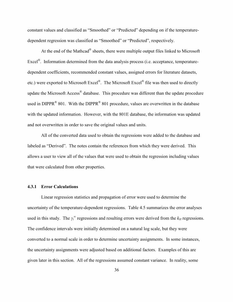
36

constant values and classified as “Smoothed” or “Predicted” depending on if the temperature-

dependent regression was classified as “Smoothed” or “Predicted”, respectively.

At the end of the Mathcad® sheets, there were multiple output files linked to Microsoft

Excel®. Information determined from the data analysis process (i.e. acceptance, temperature-

dependent coefficients, recommended constant values, assigned errors for literature datasets,

etc.) were exported to Microsoft Excel®. The Microsoft Excel® file was then used to directly

update the Microsoft Access® database. This procedure was different than the update procedure

used in DIPPR® 801. With the DIPPR® 801 procedure, values are overwritten in the database

with the updated information. However, with the 801E database, the information was updated

and not overwritten in order to save the original values and units.

All of the converted data used to obtain the regressions were added to the database and

labeled as “Derived”. The notes contain the references from which they were derived. This

allows a user to view all of the values that were used to obtain the regression including values

that were calculated from other properties.

4.3.1 Error Calculations

Linear regression statistics and propagation of error were used to determine the

uncertainty of the temperature-dependent regressions. Table 4.5 summarizes the error analyses

used in this study. The γi∞ regressions and resulting errors were derived from the kH regressions.

The confidence intervals were initially determined on a natural log scale, but they were

converted to a normal scale in order to determine uncertainty assignments. In some instances,

the uncertainty assignments were adjusted based on additional factors. Examples of this are

given later in this section. All of the regressions assumed constant variance. In reality, some

37

data are more reliable than others. Efforts were made to only include the best data in each

regression so that the assumption of constant variance was valid.

Table 4.5: Summary of uncertainty determinations for temperature-dependent regressions

Property Regression Error Analysis Assumptions kH Least squares 95% confidence intervals of the

mean (determined by regression)

Constant variance

γi∞ Thermodynamically derived

from kH, Pisat, and Ψ

Propagation of error Constant variance

xiaq Least squares 95% confidence intervals of the

mean (determined by regression)

Constant variance

Confidence intervals determined in this manner are not constant over the entire

temperature range. Confidence intervals are larger at the minimum and maximum temperatures.

In addition, for compounds that cover solid and liquid regions, the uncertainty in γi∞ tends to be

larger over the solid region versus the liquid region due to uncertainty in Ψ. In the DIPPR® 801

database, confidence intervals are assigned to the entire regression. To be consistent with the

801 database format, single uncertainties were assigned. This was accomplished by a weighted

average. First, the average absolute upper and lower percent uncertainties, s, were calculated at

every temperature for each experimental data point, j,

2

)(%)(% jdownjupj

TErrorTErrors

+= , 4.18

where %Error is the percent difference between the 95% confidence interval of the mean and the

regression value. If there were N points at a single temperature, then the uncertainty was

calculated N times. These resulting uncertainties were then averaged,

38

total

jj

N

ss∑

= , 4.19

where Ntotal is the total number of experimental points used to obtain the regression. This

resulted in greater weight for the temperatures where there were more experimental values.

These weighted absolute uncertainties were then converted to DIPPR® 801 uncertainty ranges.

The DIPPR® uncertainty options are < 0.2%, < 1%, < 3%, < 5%, <10%, < 25%, < 50%, < 100%,

and > 100%. As an example, if s = 2.7%, the uncertainty for the regression was labeled as < 3%.

When data were only available for one property, uncertainties were initially calculated as

outlined in Table 4.5. The uncertainties of the derived property regressions were then compared

to the error assigned to the regression of the original data. The derived property uncertainty was

kept if it was greater than or equal to the error of the original property data. If it was smaller, it

was changed to match the uncertainty of the original property. For example, if kH and γi∞

regressions were determined from xiaq data and the uncertainty assigned to the xi

aq regression was

< 25%, the smallest uncertainty assigned to the kH and γi∞ regressions was < 25%.

When data were only available from one reference, an uncertainty was calculated from

the regression, and this was compared to the reported author uncertainty. The largest uncertainty

of the two was reported in the database. For example, with ethyl mercaptan the uncertainty

obtained from the kH regression was < 5%. However, the uncertainty reported by the author for

the dataset was < 10%, so the uncertainty of the regression was changed to < 10%.

Uncertainties were assigned to the individual datasets based on the regression

uncertainty. Figure 4.4 shows an example of the error calculation for an experimental data point.

Each data point is at the same temperature. The points are spread along the x-axis for viewing

39

purposes. The correlation value and uncertainty are shown along with an experimental value

(shown twice). The uncertainty of the experimental value can be calculated in two different

ways as shown in the figure. The uncertainty can be taken as the difference between the

experimental and correlated values or the difference between the experimental value and

uncertainty limit of the correlated value. The latter calculation was used in this study. The

absolute uncertainties of all of the data points within a dataset were averaged to assign an overall

uncertainty to the dataset. The lowest possible uncertainty for a dataset was defined as being the

uncertainty assigned to the regression. For example, if a regression was assigned an uncertainty

of < 10% and the difference between the experimental data and regression values is 3%, the

uncertainty of the dataset was labeled as < 10%.

Figure 4.4: Uncertainty determination of experimental datasets

40

4.3.2 Critical Solution Temperatures

This section discusses compounds with upper or lower critical solution temperatures.

Table 4.6 gives the total number of compounds per chemical family with critical solution

behavior that were evaluated in this study. For the compounds with critical solution behavior,

the actual critical temperatures were not determined. The determination of the actual critical

point would involve the evaluation of xiaq and SOLC data which was beyond the scope of this

study. Term “E” in DIPPR® Equations 5000 and 6000 (see Table 4.3) was assigned a value (an

approximate critical temperature) based on the available xiaq data. This allowed the remaining

coefficients to be found using linear regression. Values should be extrapolated from

temperature-dependent equations with caution for all properties discussed in this paper. Errors

can result from extrapolation, especially for xiaq. Some of the more interesting behaviors

encountered in this study are discussed below.

Table 4.6: Chemical families with evaluated compounds exhibiting critical solution behavior

Chemical Family: Number Evaluated Compounds/Type of Critical Solution Behaviora Aldehydes: 1/UCST Nitriles: 2/UCST Aromatic Alcohols: 12/UCST Nitroamines: 1/UCST Aromatic Amines: 2/LCST Other Aliphatic Alcohols: 1/UCST Aromatic Carboxylic Acids: 1/UCST Other Aliphatic Amines: 5/LCST Cycloaliphatic Alcohols: 1/UCST Other Amines, Imines: 3/LCST Epoxides: 1/UCST Other Ethers/Diethers: 1/LCST Ketones: 1/UCST Other Polyfunctional C, H, O: 1/UCST n-Alcohols: 1/UCST Polyfunctional C, H, O, Halide: 3/UCST

aUCST = Upper Critical Solution Temperature; LCST = Lower Critical Solution Temperature

Figure 4.5 shows ln(xiaq) data plotted versus inverse temperature for 2-butanol along with

the regression obtained in this study. Below 273.15 K (0.00366 K-1), the ln(xiaq) data plateau.

The data below 273.15 K were not included in the regression due to the inability of any of the

41

equations in Table 4.4 to model the behavior with these data included. Extrapolation of the

regression below 273.15 K would obviously give erroneous xiaq values.

Figure 4.5: 2-Butanol ln(xiaq) data and regression. References: [55-62]

Figure 4.6 shows ln(xiaq) data of p-chlorophenol plotted as a function of inverse

temperature along with the regression obtained by using DIPPR® Equation 6000. The regression

was purposefully extrapolated beyond the maximum temperature in the figure to show the

dangers of extrapolation. DIPPR® Equation 6000 is not quite adequate for the xiaq behavior of p-

chlorophenol as can be seen by the residual plot in Figure 4.7. The behavior of the residuals

suggests that additional or different terms are required to correctly model the temperature-

dependence since there is a pattern in the residuals. However, since compounds like this were

the exception, DIPPR® Equation 6000 was used anyway. As already mentioned, it was desired

to have a generic equation that could apply to multiple compounds. Equations were not

42

developed for individual compounds. The error of the regression for p-chlorophenol was taken

into account with the regression statistics, and this error is reflected in the assigned uncertainty.

Figure 4.6: ln(xiaq) data and regression for p-chlorophenol. References: [63-67]

Figure 4.7: Residual plot from p-chlorophenol ln(xiaq) regression

43

4.3.3 Chemical Family Plots

Chemical family plots of temperature-dependent regressions obtained from experimental

data were used to select the best experimental datasets for a compound within the chemical

family and qualitatively check the reasonableness of the temperature trends. Temperature-

dependent chemical family plots were used throughout this project when enough data were

available for similar compounds. Most regressions within a chemical family have varying

applicable temperature ranges due to the data available for the individual compounds.

Extrapolated values based on experimental data do not always follow the trends of other

compounds within the family. When enough chemical family data were available, temperature

regressions were modified to change extrapolated behavior to better match the chemical family

trends. However, the main concern was ensuring that trends were reasonable over the

recommended temperature ranges of the regressions.

Figure 4.8 is a plot of the n-alcohol ln(xiaq) regressions (determined in this study from

experimental data) versus inverse temperature starting with 1-butanol. Smaller alcohols were not

included because of their miscibility with water. As the number of carbons (#C) increases, xiaq

decreases which is what is expected. 1-Butanol exhibited an upper critical solution temperature

in the temperature range of available data. Two regressions are shown for 1-octanol. The C8

regression is based solely on experimental data. As can be seen in the figure, the C8 regression

does not follow the same trend as the other n-alcohols. A second regression was developed (C8-

Exp&Pred) using the experimental data and predicted points based on the family trend. This

second regression was accepted.

44

Figure 4.8: n-Alcohol ln(xiaq) regressions based on experimental data versus inverse temperature.

Initial C8 regression based on experimental data (C8) and updated C8 regression based on experimental data and predicted values from the family plot (C8-Exp&Pred) are both shown.

A chemical family plot was used to determine the best kH and γi∞ data for 1-heptanol

(C7). Due to C7 SOLC values ranging between 0.285-0.334 mole fraction over the temperature

range of 278.15-333.15 K [58, 59], xiaq data were not included in the kH and γi

∞ regressions.

However, xiaq data were still helpful in identifying the best datasets. C7 literature values plotted

as ln(kH) versus inverse temperature are shown in Figure 4.9. The 1-hexanol and 1-octanol (C6

and C8) kH regressions were also used to identify the best datasets. The data from reference a

[47] and the values reported from one of the experimental methods used in reference c [68] agree

with the average of the C6 and C8 regressions (Avg C6 & C8). These two references also agree

with the literature xiaq data. Predicted values from the average of the C6 and C8 regressions at

45

temperatures higher and lower than the available C7 data were included in the regression so the

extrapolated behavior better matched the family behavior.

Figure 4.9: 1-Heptanol values plotted as ln(kH) versus inverse temperature. 1-Octanol (C8) and 1-hexanol (C6) regressions obtained from experimental data shown along with the average of these two regressions (Avg C6 & C8). References: a [47], b [69], c [68] (*reference reports values using two different experimental methods), d [70], e [71], xi

aq data [44, 72-80]

Figure 4.10 is a plot of ln(γi∞) regressions versus inverse temperature for the n-alcohols.

Values in the figure are plotted within the recommended temperature ranges of each regression;

however, extrapolated trends were considered. Initially all of the regressions were developed

based solely on experimental data. The larger n-alcohols have fewer data with more scatter than

the smaller n-alcohols. As a result, the regressions have larger uncertainties. For 1-octanol (C8),

curvature was not significant over the temperature range of the data, so extrapolated values did

46

not match the shape of the other compounds. Predicted values were combined with the C8

experimental data to obtain curves for γi∞ and kH (C8-Exp&Pred). As was mentioned, predicted

values were also combined with the C7 experimental data to help with extrapolation. The

change in the regression due to the predicted points was not as drastic for C7 as with C8, so it is

not shown in the plot. As #C increases, γi∞ values increase meaning that deviations from

ideality are increasing. As the carbon chain grows, the molecules become more hydrophobic.

Figure 4.11 is a plot of the ln(kH) regressions for the n-alcohols shown over extrapolated

temperature ranges. The same data used to obtain the regressions shown in Figure 4.10 were

used to obtain the kH regressions. As was seen with γi∞ for 1-octanol, the initial regression based

only on experimental data (C8) extrapolated differently from the other compounds. The “8-

Exp&Pred regression follows the chemical family trend at higher temperatures. The difference

between the kH temperature-dependent behavior of the C8 and C8-Exp&Pred regressions is very

noticeable in Figure 4.11. As with the γi∞ values, as #C increases, kH values increase. However,

the influence of temperature is greater on kH than γi∞. It has been noted that changes in kH are

small in a chemical family when compared to xiaq and Pi

sat [19]. This is especially obvious at

lower temperatures with the n-alcohols. Since xiaq and γi

∞ are inversely related for liquids (see

Equation 4.4), then changes in γi∞ will also be larger in a chemical family than changes in kH.

These trends are also observed with the n-alcohol regressions.

47

Figure 4.10: n-Alcohol ln(γi∞) regressions based on experimental data versus inverse temperature

Figure 4.11: n-Alcohol ln(kH) regressions based on experimental data versus inverse temperature

48

4.3.4 Other Data Analysis Notes

For some compounds, γi∞ or kH values are reported from xi

aq measurements, but the Pisat

and/or Ψ values used in the literature were significantly different from those calculated in this

study. In these instances, γi∞ and kH values were recalculated from the original xi

aq values using

DIPPR®801 properties and the values reported in the literature were not used.

4.4 Constant Values

Temperature-dependent data are not available for every compound, so chemical family

plots were used to evaluate compounds with data only available at 298.15 K. Plots of the natural

log of xiaq or γi

∞ often are a linear function of carbon number (#C) [81, 82]. These plots use a

group contribution approach (discussed in more detail in Section 7.1). If a plot is created in

which a unit on the x-axis represents the addition of a molecular group (which in this study was

typically chosen to be –CH2-), the property will change in incremental values with the number of

groups. If there is a functional group that is similar to all compounds, it does not have to be

explicitly included on the x-axis. For example, a linear trend can be observed for n-alcohols

where the x-axis only takes into account the #C. Since all compounds have a hydroxyl group on

C1, this functional group is inherently accounted for in the plot. These types of family plots

were used to either smooth values as a function of #C or designate the best experimental values

based on the family trend. The property that was chosen for the family plots was the property

that had the best linear correlation (highest R2 value) for the natural log of the property plotted as

a function of #C.

49

4.4.1 Chemical Family Plot Regressions

Within a chemical family, some of the compounds had enough data to perform

temperature-dependent evaluations (see Section 4.3) while other compounds only had data at a

single temperature. In these instances, “Smoothed” values (determined by evaluating the

temperature-dependent regressions at 298.15 K) were combined with the available literature data

at 298.15 K of the unevaluated compounds to obtain a regression of the natural log of a property

as a function of #C. Recommended values were then determined for each unevaluated #C using

the regression. This method was used when most of the compounds in a chemical family already

had recommended values from evaluating temperature-dependent data. In other instances, all of

the original data at 298.15 K were used within a chemical family to obtain a regression of the

natural log of a property as a function of #C. Since every chemical family was handled uniquely

due to the availability of data, notes about the data used to determine recommended values from

family plots were included in the database with the “Smoothed” values. Examples of this data

evaluation process and chemical families with interesting behavior are included below.

The constant value family plot for the 1-alkenes is an example of using all of the

literature data in the evaluation process. Temperature-dependent evaluations were not performed

for any of the liquid 1-alkenes due to the limited amount of temperature-dependent data.

Literature kH and xiaq data at 298.15 K for the 1-alkenes are plotted as ln(xi

aq) versus #C in Figure

4.12. The data show a linear relationship between ln(xiaq) and #C (R2 = 0.997). A linear

regression was used to obtain recommended xiaq values at 298.15 K and labeled as “Smoothed”

for each #C of the chemical family. The 95% confidence intervals of the mean (as determined

by the regression) were used to determine the uncertainty of the “Smoothed” values. Values

were predicted for C10-C14 by interpolation and labeled as “Predicted”. The recommended 1-

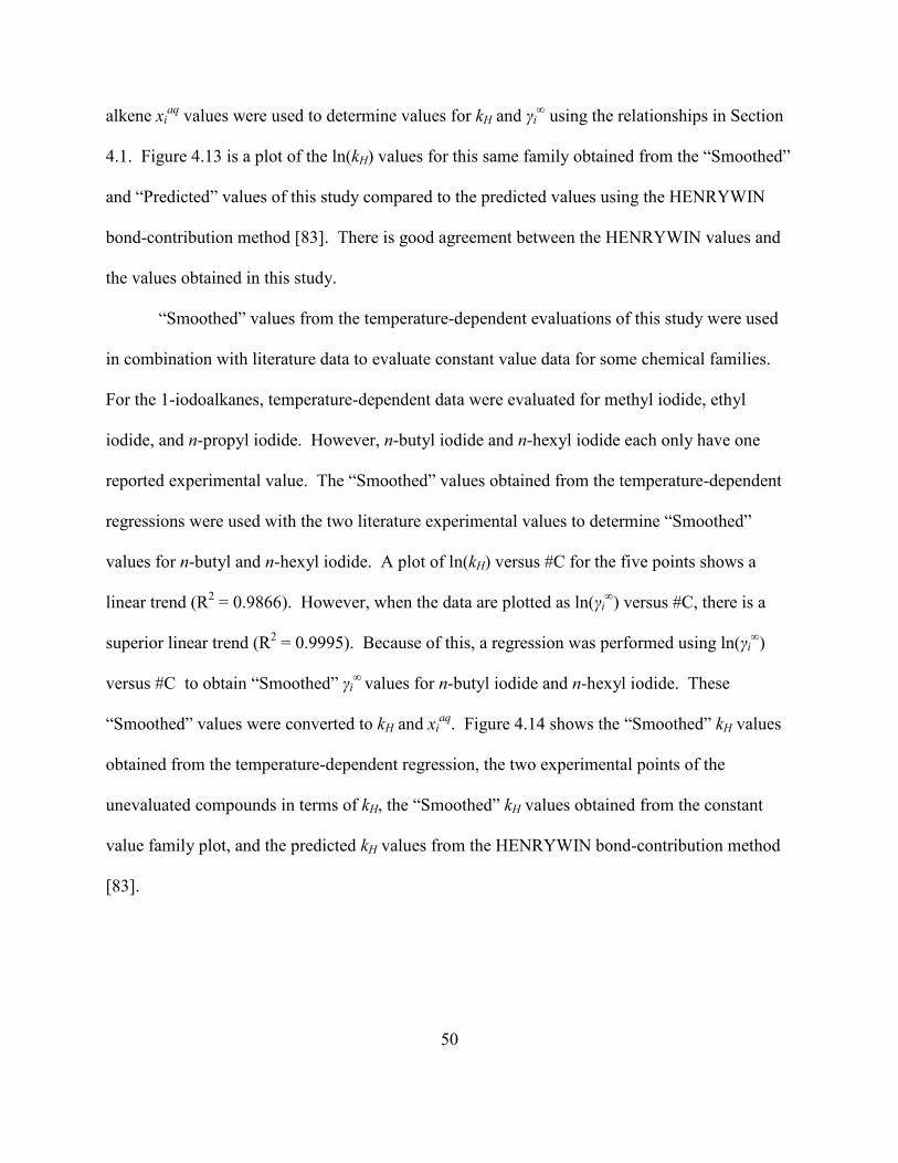
50

alkene xiaq values were used to determine values for kH and γi

∞ using the relationships in Section

4.1. Figure 4.13 is a plot of the ln(kH) values for this same family obtained from the “Smoothed”

and “Predicted” values of this study compared to the predicted values using the HENRYWIN

bond-contribution method [83]. There is good agreement between the HENRYWIN values and

the values obtained in this study.

“Smoothed” values from the temperature-dependent evaluations of this study were used

in combination with literature data to evaluate constant value data for some chemical families.

For the 1-iodoalkanes, temperature-dependent data were evaluated for methyl iodide, ethyl

iodide, and n-propyl iodide. However, n-butyl iodide and n-hexyl iodide each only have one

reported experimental value. The “Smoothed” values obtained from the temperature-dependent

regressions were used with the two literature experimental values to determine “Smoothed”

values for n-butyl and n-hexyl iodide. A plot of ln(kH) versus #C for the five points shows a

linear trend (R2 = 0.9866). However, when the data are plotted as ln(γi∞) versus #C, there is a

superior linear trend (R2 = 0.9995). Because of this, a regression was performed using ln(γi∞)

versus #C to obtain “Smoothed” γi∞ values for n-butyl iodide and n-hexyl iodide. These

“Smoothed” values were converted to kH and xiaq. Figure 4.14 shows the “Smoothed” kH values

obtained from the temperature-dependent regression, the two experimental points of the

unevaluated compounds in terms of kH, the “Smoothed” kH values obtained from the constant

value family plot, and the predicted kH values from the HENRYWIN bond-contribution method

[83].

51

Figure 4.12: 1-Alkene kH and xiaq data at 298.15 K plotted as ln(xi

aq) versus carbon number (#C). References: [47, 72, 84-87]

Figure 4.13: 1-Alkene ln(kH) values at 298.15 K from this study (“Smoothed” and “Predicted”) and HENRYWIN bond-contribution prediction method [83] plotted as a function of carbon number (#C)

52

Figure 4.14: 1-Iodoalkane ln(kH) values at 298.15 K from temperature-dependent regressions (Temp. Dep. Smoothed), constant value family plot (Const. Val. Smoothed), the literature (data) [47], and HENRYWIN bond-contribution method [83] plotted as a function of carbon number (#C)

Figure 4.15 shows “Smoothed” values obtained from temperature-dependent evaluations

for the C4-C10 n-alcohols and literature values for the C11 and larger n-alcohols. Data at

temperatures ranging between 277.15 K and 307.15 K were included due to the limited data

available for the larger compounds. The values that are at 298.15 K have solid backgrounds.

Possible reasons for the scatter in the literature data include difficulties with accurately

measuring small concentrations, the addition of trace amounts of salts by some authors in order

to prevent microbial degradation of the alcohol (references c [88] and f [89]), and varying

temperatures (xiaq values are expected to be smaller at lower temperatures). The C16 and C17

data of reference d [90] suggests that the xiaq values eventually plateau as a function of #C.

However, the authors of reference d [90] report that the C17 xiaq value is less than or equal to the

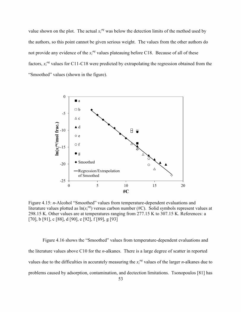
53

value shown on the plot. The actual xiaq was below the detection limits of the method used by

the authors, so this point cannot be given serious weight. The values from the other authors do

not provide any evidence of the xiaq values plateauing before C18. Because of all of these

factors, xiaq values for C11-C18 were predicted by extrapolating the regression obtained from the

“Smoothed” values (shown in the figure).

Figure 4.15: n-Alcohol “Smoothed” values from temperature-dependent evaluations and literature values plotted as ln(xi

aq) versus carbon number (#C). Solid symbols represent values at 298.15 K. Other values are at temperatures ranging from 277.15 K to 307.15 K. References: a [70], b [91], c [88], d [90], e [92], f [89], g [93]

Figure 4.16 shows the “Smoothed” values from temperature-dependent evaluations and

the literature values above C10 for the n-alkanes. There is a large degree of scatter in reported

values due to the difficulties in accurately measuring the xiaq values of the larger n-alkanes due to

problems caused by adsorption, contamination, and dectection limitations. Tsonopoulos [81] has

54

noted that ln(xiaq) for the n-alkanes is a linear function of #C up until n-nonane. As #C increases

beyond C9, ln(xiaq) continues to decrease but at a smaller rate. Most of the experimental data

indicate that the there is an eventual plateau in xiaq values. One theory is that the folding of the

larger chain n-alkanes causes this plateau. Ferguson et al.[94] disagree with this theory and

claim that the experimental data are erroneous. They used molecular dynamic simulations to

study the xiaq of n-alkanes and found that there is an exponential decrease in xi

aq up to C20. This

theory better matches the trend observed with the n-alcohols (Figure 4.15). Due to the

agreement of the molecular simulations and the n-alcohol trend, the data of Tolls et al. [95]

(points are highlighted in Figure 4.16) were recommended in this study. Future experimental

work would be helpful in better understanding this chemical family trend.

Figure 4.17 shows “Smoothed” and literature xiaq values for the n-alkylbenzenes plotted

as a function of #C. Tsonopolous has noted slight curvature as ln(xiaq) data are plotted as a

function of #C for the n-alkylbenzenes [82]. Because of this, a quadratic equation was used to

smooth the data instead of linear equation. The value at C19 suggests that the quadratic trend

does not continue after C16. The xiaq values of large hydrocarbons are difficult to measure due to

the small concentration, so more xiaq values of the large n-alkylbenzenes need to be measured in

order to confidently understand the curvature after C16. “Smoothed” values obtained from

temperature-dependent regressions were included in the constant value regression for C6-C12.

The available data point at C16 was also included, but the data points at C13 and C14 were

rejected because they do not agree with the family plot. Values for C13-C16 were determined

from smoothing these combined values.

55

Figure 4.16: n-Alkane “Smoothed” values from temperature-dependent evaluations and literature (Data) xi

aq values at 298.15 K. References: [85, 95-104]

Figure 4.17: n-Alkylbenzene ln(xiaq) values at 298.15 K from temperature-dependent regressions

(Temp. Dep. Smoothed), constant value family plot (Const. Val. Smoothed), and the literature (Data) plotted as a function of carbon number (#C). References: [105, 106]

56

When analyzing the di-n-alkyl phthalates, only three of the compounds (dimethyl,

diethyl, and di-n-butyl phthalates) had temperature-dependent data. These three phthalates were

evaluated using the procedure discussed in Section 4.3. The remaining phthalates only have

literature xiaq data at ambient conditions. Figure 4.18 is a plot of ln(xi

aq) at 298.15 K as a

function of the number of carbons on the alkyl chains (#C). The linear relationship between

ln(xiaq) and #C was used to provide recommended values for di-n-propyl and di-n-hexyl

phthalates, #C = 6 and #C = 12, respectively. A linear regression was performed with the

temperature-dependent “Smoothed” values and the data shown in Figure 4.18. Two literature

values were rejected because they did not follow the linear relationship like the remaining data.

This regression was used to determine “Smoothed” values for di-n-propyl and di-n-hexyl

phthalates.

Figure 4.18: di-n-Alkyl phthalate ln(xiaq) values at 298.15 K from temperature-dependent

regressions (Temp. Dep. Smoothed), constant value family plot (Const. Val. Smoothed), and the literature (Data and Rejected Data) plotted as a function of the number of carbons on the alkyl chains (#C). References: [107-115]

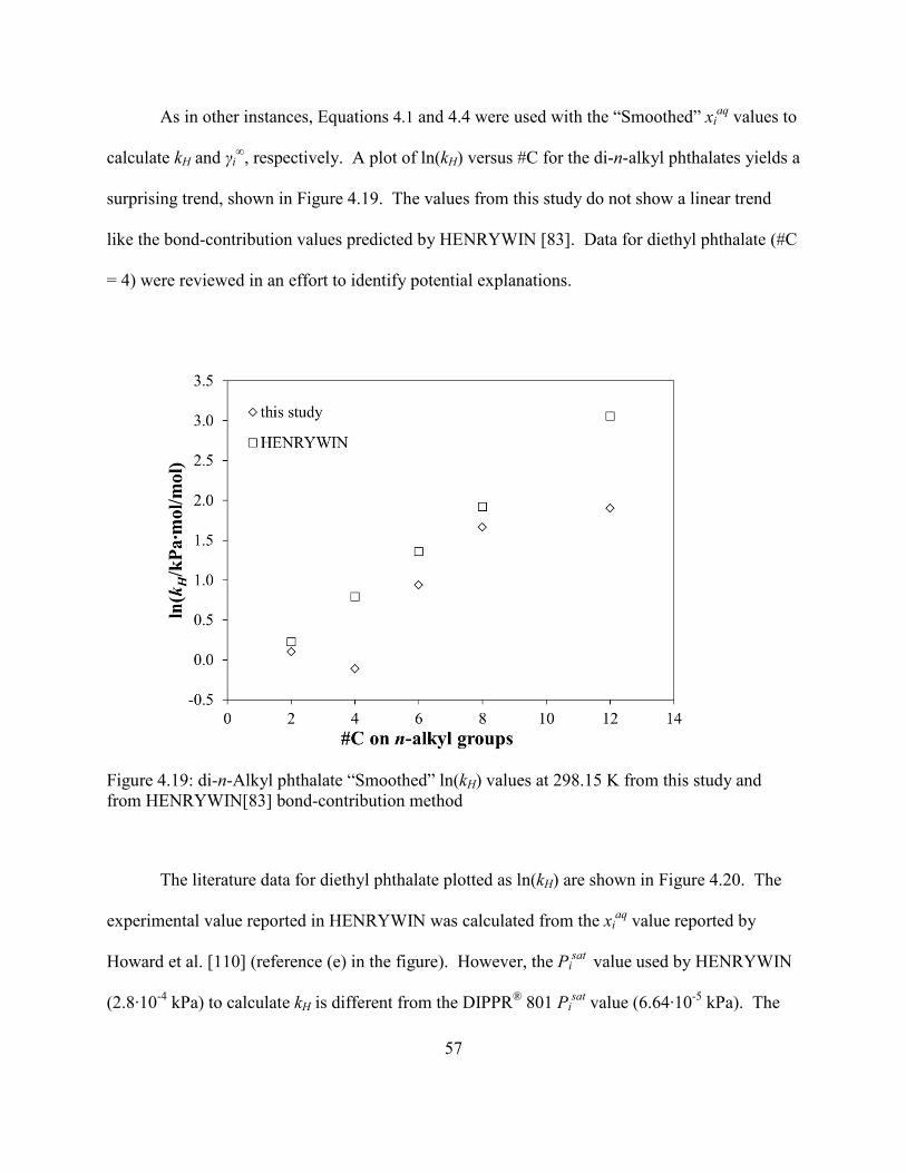
57

As in other instances, Equations 4.1 and 4.4 were used with the “Smoothed” xiaq values to

calculate kH and γi∞, respectively. A plot of ln(kH) versus #C for the di-n-alkyl phthalates yields a

surprising trend, shown in Figure 4.19. The values from this study do not show a linear trend

like the bond-contribution values predicted by HENRYWIN [83]. Data for diethyl phthalate (#C

= 4) were reviewed in an effort to identify potential explanations.

Figure 4.19: di-n-Alkyl phthalate “Smoothed” ln(kH) values at 298.15 K from this study and from HENRYWIN[83] bond-contribution method

The literature data for diethyl phthalate plotted as ln(kH) are shown in Figure 4.20. The

experimental value reported in HENRYWIN was calculated from the xiaq value reported by

Howard et al. [110] (reference (e) in the figure). However, the Pisat value used by HENRYWIN

(2.8∙10-4 kPa) to calculate kH is different from the DIPPR® 801 Pisat value (6.64∙10-5 kPa). The

58

experimental value reported in HENRYWIN is shown on Figure 4.20 with the bond-contribution

value. Both HENRYWIN values are significantly different from the values used in this study.

Values in this study are considered superior due to the reviewed Pisat values available in DIPPR®

801. As can be seen by this example, the quality of kH values determined using xiaq is largely

dependent on the quality of Pisat values used.

Figure 4.20: Literature data of diethyl phthalate at 298.15 K plotted as ln(kH) compared with HENRYWIN bond-contribution value and reported experimental value [83]. References: a [111], b [116], c [109], d [112], e [110], f [107]

The discrepancy between Pisat values for diethyl phthalate does not fully explain the

interesting kH trend observed in this study. Taking the natural log of Equation 4.1 results in

)ln()ln()ln( aqi

satiH xPk −= . 4.20

59

Equation 4.20 explains how a nonlinear trend is obtained from two relatively linear trends.

Figure 4.21 shows ln(Pisat) and ln(xi

aq) on the same plot. Both properties have linear trends with

R2 > 0.99. For the two smallest compounds, ln(Pisat) and ln(xi

aq) are very similar to each other

meaning that ln(kH) is close to 0. For all of the compounds except diethyl phthalate, ln(Pisat) is

larger than ln(xiaq) resulting in a positive ln(kH). For diethyl phthalate, ln(Pi

sat) is slightly smaller

than ln(xiaq) which leads to a negative ln(kH). If ln(Pi

sat) and ln(xiaq) were completely linear

functions of #C, then ln(kH) would exhibit a completely linear trend. The values obtained in this

study were accepted despite the unusual trend. Either more experimental data are necessary to

find a better trend, or kH values for this chemical family are not modeled very well using a group

contribution approach.

Figure 4.21: Smoothed ln(xiaq) and ln(Pi

sat) [117] of di-n-alkyl phthalates at 298.15 K

60

Temperature-dependent kH and xiaq data were available for the C5, C6, and C8

cycloalkanes, allowing for the determination of temperature-dependent regressions. Only limited

xiaq data are available for C7. Values obtained from the regressions at 298.15 K were analyzed

with the data for C7. A ln(xiaq) family plot was used to predict xi

aq for C7 which was then used

to calculate kH and γi∞ values for this compound. (The reported xi

aq value at 298.15 K did not

agree with the family plot, so it was rejected.) Similarly, for the C5-C8 cycloalkenes, all but C7

had temperature-dependent kH and xiaq values. A family plot showed that the reported xi

aq value

for C7 at 298.15 K agrees with the values for the other compounds. This xiaq value was accepted

and used to determine kH and γi∞at 298.15 K. The ln(xi

aq) values for the cycloalkanes and

cycloalkenes are shown in Figure 4.22 with ln(Pisat) values shown on the same figure. The

cycloalkanes and cycloalkenes both become less soluble in water as #C increases. The

cycloalkanes are less soluble than the cycloalkenes which is because of the presence of the

double bond in the cycloalkenes.

Figure 4.23 shows cycloalkane and cycloalkene ln(kH) values accepted from this study

compared to HENRYWIN bond-contribution values [83]. The values in this study do not

increase with #C as predicted by HENRWIN; the values are fairly constant for each of the

families. This is explained by the ln(xiaq) and ln(Pi

sat) trends shown in Figure 4.22. The two

properties have fairly parallel trends to each other for each chemical family (and even between

families). The difference between two parallel lines is a constant. Since, ln(kH) is the difference

between these parallel trends (see Equation 4.20), the ln(kH) values are fairly constant. As shown

with the n-alcohol example (Section 4.3.3), the difference between kH values within a chemical

family is much smaller than the difference in xiaq or γi

∞.

61

Figure 4.22: Cycloalkane and cycloalkene ln(xiaq) and ln(Pi

sat) values at 298.15 K plotted as a function of carbon number (#C). References: [86, 117]

Figure 4.23: Cycloalkane and cycloalkene ln(kH) values at 298.15 K compared to HENRYWIN bond-contribution values [83]

62

4.4.2 Averaging

For some compounds it was difficult or impossible to do a family plot due to the

unavailability of data for compounds with similar structures. For some compounds, the reported

values at 298.15 K were averaged when multiple reported values are in good agreement with

each other. In this case, the error was related to the standard deviation of the average. For

example, kH and γi∞ values are only available for triethylamine at 298.15 K. These values look

reasonable compared to xiaq data at that temperature (Figure 4.24). However, xi

aq data were not

used to obtain temperature-dependent equations for kH and γi∞ due to the relatively high SOLC

and the lower critical solution behavior. Instead, averages were taken of the available kH and γi∞

values after conversion to the same property. The standard deviation of the literature data at this

temperature is less than 5%.

Figure 4.24: Triethylamine xiaq, γi

∞, and kH literature data. References: [118-127]

63

Another example of this data analysis technique is with 2,3,4-trimethylpentane. Only xiaq

data are reported for this compound. Of the available xiaq data, only one reference provides

temperature-dependent data. However, the value at 298.15 K from the reference with

temperature-dependent data does not line up with three additional references. In this instance,

the three xiaq values at 298.15 K that are in agreement with each other were averaged and used to

derive kH and γi∞.

4.5 American Petroleum Institute Recommendations

The American Petroleum Institute (API) Technical Data Book [128] provides

recommended temperature-dependent kH values for various compounds. For gases, API

recommendations are based on values measured at multiple pressures. Due to the structure of the

801E database, data were entered only as a function of temperature and not pressure. Only data

for gases at a pressure of 1 atm were included. The wider range of data for gases used in the API

regressions renders their recommendations more reliable than what could be done in this study.

In addition, the API evaluations for select liquids were determined to be reliable. As such, API

recommendations for 31 compounds (26 gases and 5 liquids) were accepted in this study and are

represented in the compound totals given in Table 3.2 and Table 3.3.

API temperature dependent coefficients were reported for kH in the form of DIPPR® 801

Equation 101 (see Table 4.3). Using the relationship between kH and xiaq for gases leads to

)ln()325.101ln()ln( aqiH xk −= . 4.21

Since ln(101.325) is a constant, coefficients can be derived from the API coefficients to develop

a temperature dependent equation for xiaq. A similar relationship was given for liquids in

Equation 4.20. Since Pisat is in the form of DIPPR® Equation 101 as well, the API kH and

64

DIPPR® 801 Pisat coefficients were combined to determine xi

aq coefficients for liquids.

Equations obtained from API equations were classified as “Derived” instead of “Smoothed”.

API regression errors are reported in various forms. The errors had to be converted to the

error notation used in DIPPR® 801. If the API error was reported as an average absolute

deviation (AAD) then the regression was assigned the corresponding error in the database. For

example, if AAD = 5.88%, then the error reported in the database is < 10%. If the API error was

reported on a log scale (i.e. standard deviation in ln(xiaq) is 1.8%) then the property was

calculated at N points evenly distributed along the temperature range where N is the number of

values that were used to obtain the regression. The upper and lower uncertainty limits were

calculated at these points on the normal scale, and the AAD was determined at each point. These

AADs were averaged and an overall error code was assigned based on this average. The same

error was assigned to xiaq and kH regressions of the same compound.

API recommendations were accepted without ensuring that all of the data used in the

original regression were present in the 801E database. Many of the references included in the

API database were included in this study. However, the API database used high pressure data

which were purposefully excluded from this study. Uncertainties of the datasets in this database

were determined from the reported regression uncertainty in the same manner that uncertainties

were assigned in Section 4.3.1.

4.6 Comparison with Literature Recommendations and Predicted Values

The temperature regressions obtained in this study were compared with available

recommendations such as the IUPAC-NIST Solubility Data Series [129-165], API Technical

Data Book [128], and other literature reviews. This was done to validate the evaluation

65

procedure used in this study and to ensure that the recommended regressions of this study reflect

the data included in the 801E database. Except for the API regressions mentioned in Section 4.5,

outside regressions were not accepted so that a future database user can view the datasets that

were used to develop the regression.

The IUPAC-NIST equation uses empirical constants that were obtained from

simultaneous regression of all of the xiaq data for compounds within a certain chemical family

[166]. Data were then classified as “Recommended”, “Tentative”, “Doubtful”, or “Rejected”

based on the error between the regression equation and the actual literature data [150]. These

classifications are given per point and not per reference; whereas, in this study, all of the points

from a given reference were accepted or rejected unless there was a valid reason to split a data

set (for example, the experimental method is not as accurate in a certain temperature or

concentration region). In this study, temperature regressions were based solely on literature data.

If the agreement between the regressions of this study and those published was within the

regression uncertainty, the parameters in this study were immediately accepted. In instances

where the disagreement was larger than the regression uncertainty, the regressions were

compared more judiciously. Insights gained through thermodynamic relationships, chemical

family trends, and predicted values (as previously discussed) were useful in determining the best

values when there were discrepancies.

In order to ensure that the analyses performed in this study were reasonable when

derivative properties were excluded, recommended values determined in this study were

compared to recommendations given in the literature that included derivative properties. As an

example, Figure 4.25 shows methanol literature γi∞ and kH values plotted as ln(γi

∞), the regression

obtained in this study, and the regression recommended by Dohnal et al. [21]. The 95%

66

confidence intervals for the regression from this study are also shown. In the analysis performed

by Dohnal et al. [21], the temperature-dependent parameters were obtained by simultaneously

fitting γi∞, limiting partial molar excess enthalpy, and limiting partial molar heat capacity data.

Their analysis included more properties than this study. However, their regression is within the

uncertainty of the regression from this study. As an additional example, the evaluations by

Plyasunov et al. [21-26] included derivative properties. Values at 298.15 K from this study were

compared to their recommendations for approximately 150 compounds. The recommendations

of this study are all within the reported uncertainties. These comparisons provided confidence

that the properties and evaluation procedure used in this study produce reliable regressions.

Figure 4.25: Methanol γi∞ regressions from this study and Dohnal et al. [21]. References: [45, 48,

69, 70, 77, 167-182]

67

The regressions of this study do not always match the regressions reported in the IUPAC-

NIST solubility data series. Figure 4.26 shows literature xiaq data for n-propyl formate, the

regression obtained in this study, and the regression reported in the IUPAC-NIST Solubility Data

Series [159]. The confidence intervals correspond to the average absolute error of the regression

obtained in this study (see Section 4.3.1). In addition, the figure shows xiaq data for ethyl formate

for comparison purposes. The IUPAC-NIST regression extrapolates very differently from the

regression in this study. However, over the temperature range of experimental data (which is the

recommended range of the regression) the regressions are not statistically different. The

regression of this study was accepted in the database. Similar trends were observed with

additional compounds, and these compounds were handled in the same manner.

Figure 4.26: n-Propyl formate xiaq data, regression from this study, and IUPAC-NIST [159]

regression compared to ethyl formate xiaq data. References: [183, 184]

68

Figure 4.27 is an example that shows how data from the combined properties help in the

data analysis process. The xiaq data for di-n-propyl ether are shown along with xi

aq values

calculated from literature kH and γi∞ data. All of the xi

aq data were reported in the same paper,

but two experimental methods were used. The xiaq dataset that does not agree with the kH and γi

∞

data were measured using a less reliable method, so those points were rejected. The kH, γi∞, and

remaining xiaq data were used to obtain the regression shown in the plot. The IUPAC-NIST

[158] trend is also shown, and it is significantly different over the entire temperature range. All

of the IUPAC-NIST ether trends use theoretical coefficients, and all ether systems (except one)

are forced to exhibit a minimum at 360 K [185]. The regression of this study is recommended

because it matches experimental data from multiple references and properties.

Figure 4.27: di-n-Propyl ether xiaq regressions from this study and from IUPAC-NIST [158].

References: [47, 172, 186-189]

69

Another example is shown below (Figure 4.28) where the regressions are significantly

different over part of the data range. The figure shows literature xiaq data for 3-methyl-3-

pentanol, the regression obtained in this study with the average confidence intervals, and the

regression reported in the IUPAC-NIST Solubility Data Series [150]. Some of the data were

rejected because the data are old (measured in 1938), and the experimental and analytical

methods used are not as reliable as the methods used with the more recent data. The IUPAC-

NIST regression shows significantly different behavior as temperature increases. The regression

from this study was accepted because it follows the available experimental data.

Figure 4.28: 3-Methyl-3-pentanol xiaq regressions from this study and from IUPAC-NIST [150].

References: [44, 190]

70

In the following examples, kH values predicted using the group contribution method of

Sedlbauer et al. [191] were used to help identify the best datasets. The Sedlbauer et al. [191]

method was developed using data for multiple hydrocarbons, so it can be used reliably to identify

the best datasets for similar types of compounds. Values were converted between xiaq and kH

using Equation 4.1 and DIPPR® 801 [117] Pisat data.

When the data evaulation methods already discussed were not helpful in distinguishing

between conflicting data sets for a compound, prediction methods (discussed in Chapter 7) were

helpful in identifying the best datasets. As an example, with cumene there are multiple xiaq

temperature trends shown by literature data (Figure 4.29). More data are available in the

literature for this compound than are shown in the figure; however, there is enough scatter in

these additional data that they do not aid in identifying the best trend. These additional datasets

were included in data analysis, but they are not shown in the figure for viewing purposes. The

predicted Sedlbauer et. al [191] values (kH converted to xiaq) and IUPAC-NIST [136] curve are

the closest to the data from reference b [192] while the API [128] regression is based on the data

of reference c [193]. The IUPAC-NIST [136] trend is based on xiaq data for multiple

hydrocarbons. The prediction method of Sedlbauer et al. [191] was developed using data for

multiple aromatic hydrocarbons, so the trend inherently takes into account chemical family

trends. The relative agreement between the Sedlbauer et al. [191] and IUPAC-NIST [136]

recommendations is encouraging because both used information gained from examining multiple

compounds with similar structures. Because of this, the data from reference b [192] are

recommended.

71

Figure 4.29: Cumene xiaq data compared with Sedlbauer et. al [191] predicted values and API

[128] and IUPAC-NIST [136] recommendations. References: a [194], b [192], c [193], d [105]

As another example, limited data are available for 2,2,5-trimethylhexane. The available

literature xiaq values are plotted as ln(kH) versus inverse temperature in Figure 4.30 with kH

values predicted using the group contribution method developed by Sedlbauer et al. [191]. Data

for this compound were not included in the Sedlbauer et al. [191] method development; however,

data for other aliphatic hydrocarbons were included making the method applicable for this

compound. The difference between the two reported values at 298.15 K (0.00335 K-1 on the

inverse temperature scale) make it difficult to identify the best values by looking at the data

alone. The predicted values are in agreement with the data points reported by reference a [195],

so these values were accepted.

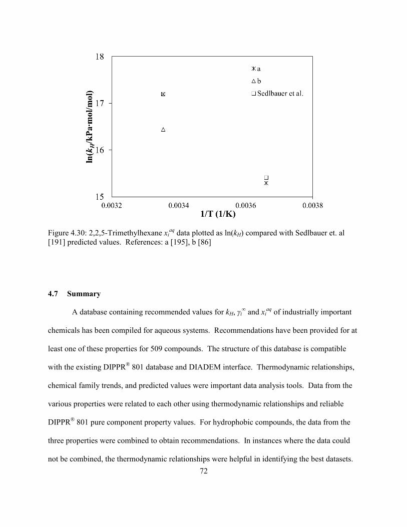
72

Figure 4.30: 2,2,5-Trimethylhexane xiaq data plotted as ln(kH) compared with Sedlbauer et. al

[191] predicted values. References: a [195], b [86]

4.7 Summary

A database containing recommended values for kH, γi∞ and xi

aq of industrially important

chemicals has been compiled for aqueous systems. Recommendations have been provided for at

least one of these properties for 509 compounds. The structure of this database is compatible

with the existing DIPPR® 801 database and DIADEM interface. Thermodynamic relationships,

chemical family trends, and predicted values were important data analysis tools. Data from the

various properties were related to each other using thermodynamic relationships and reliable

DIPPR® 801 pure component property values. For hydrophobic compounds, the data from the

three properties were combined to obtain recommendations. In instances where the data could

not be combined, the thermodynamic relationships were helpful in identifying the best datasets.

73

Chemical family plots were used with temperature-dependent and single-temperature data to

check for consistency within chemical families and to select the best data. Predicted values were

used to select the best datasets when there were discrepancies in the literature data. Notes in the

database provide information about the procedure and data used to provide recommendations for

each compound and property.

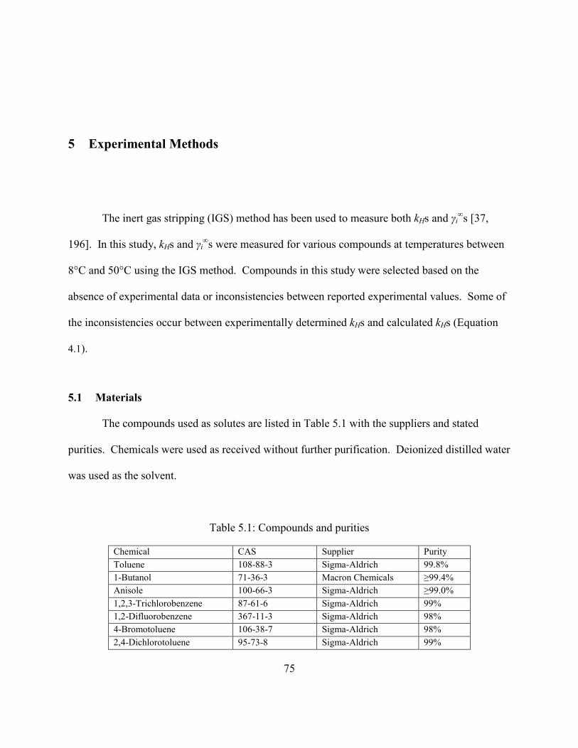
75

5 Experimental Methods

The inert gas stripping (IGS) method has been used to measure both kHs and γi∞s [37,

196]. In this study, kHs and γi∞s were measured for various compounds at temperatures between

8°C and 50°C using the IGS method. Compounds in this study were selected based on the

absence of experimental data or inconsistencies between reported experimental values. Some of

the inconsistencies occur between experimentally determined kHs and calculated kHs (Equation

4.1).

5.1 Materials

The compounds used as solutes are listed in Table 5.1 with the suppliers and stated

purities. Chemicals were used as received without further purification. Deionized distilled water

was used as the solvent.

Table 5.1: Compounds and purities

Chemical CAS Supplier Purity Toluene 108-88-3 Sigma-Aldrich 99.8% 1-Butanol 71-36-3 Macron Chemicals ≥99.4% Anisole 100-66-3 Sigma-Aldrich ≥99.0% 1,2,3-Trichlorobenzene 87-61-6 Sigma-Aldrich 99% 1,2-Difluorobenzene 367-11-3 Sigma-Aldrich 98% 4-Bromotoluene 106-38-7 Sigma-Aldrich 98% 2,4-Dichlorotoluene 95-73-8 Sigma-Aldrich 99%

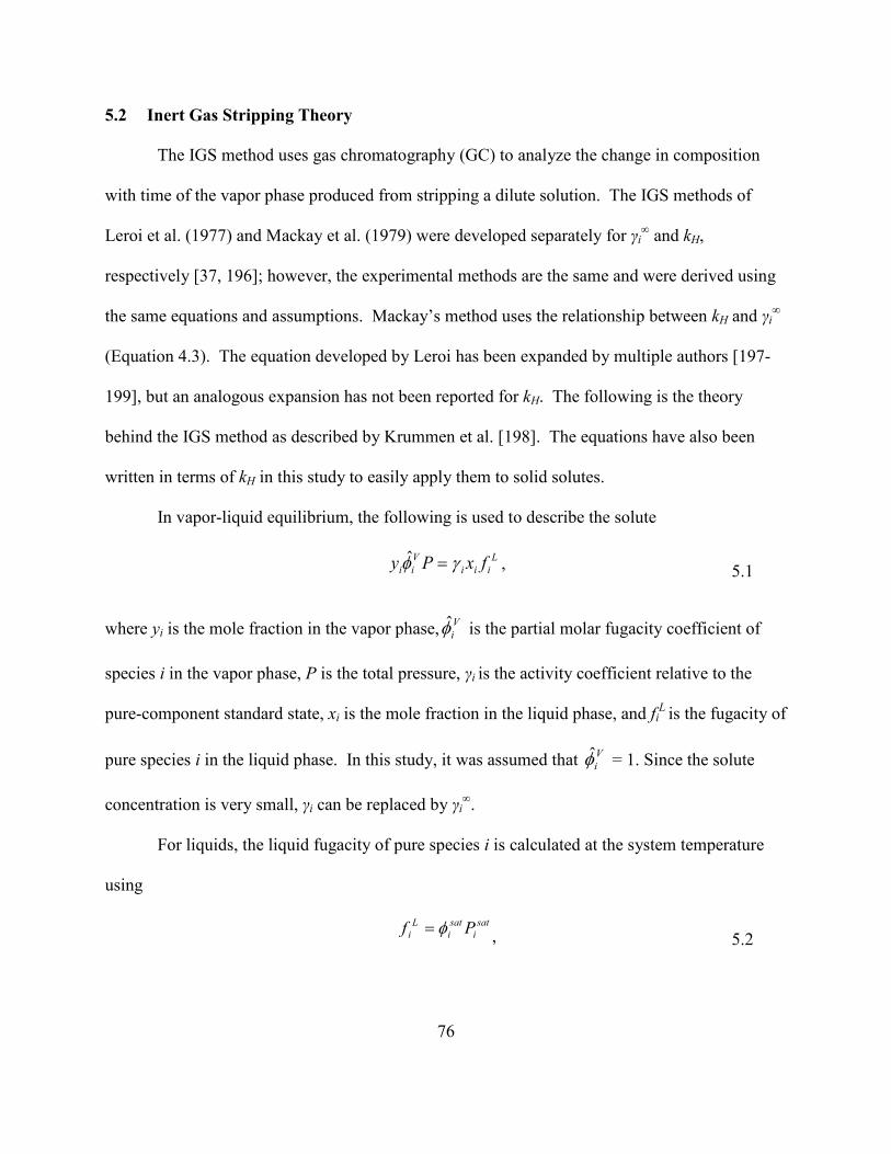
76

5.2 Inert Gas Stripping Theory

The IGS method uses gas chromatography (GC) to analyze the change in composition

with time of the vapor phase produced from stripping a dilute solution. The IGS methods of

Leroi et al. (1977) and Mackay et al. (1979) were developed separately for γi∞ and kH,

respectively [37, 196]; however, the experimental methods are the same and were derived using

the same equations and assumptions. Mackay’s method uses the relationship between kH and γi∞

(Equation 4.3). The equation developed by Leroi has been expanded by multiple authors [197-

199], but an analogous expansion has not been reported for kH. The following is the theory

behind the IGS method as described by Krummen et al. [198]. The equations have also been

written in terms of kH in this study to easily apply them to solid solutes.

In vapor-liquid equilibrium, the following is used to describe the solute

Liii

Vii fxPy γφ =ˆ , 5.1

where yi is the mole fraction in the vapor phase, Viφ̂ is the partial molar fugacity coefficient of

species i in the vapor phase, P is the total pressure, γi is the activity coefficient relative to the

pure-component standard state, xi is the mole fraction in the liquid phase, and fiL is the fugacity of

pure species i in the liquid phase. In this study, it was assumed that Viφ̂ = 1. Since the solute

concentration is very small, γi can be replaced by γi∞.

For liquids, the liquid fugacity of pure species i is calculated at the system temperature

using

sat

isati

Li Pf φ= , 5.2

77

where Pisat is the vapor pressure and sat

iφ is the vapor-phase fugacity coefficient of pure species i

at its saturation pressure. This equation assumes the Poynting factor is unity which is valid at

atmospheric pressure. Substituting Equation 5.2 into 5.1 gives

sati

satiiii PxPy φγ ∞= . 5.3

The vapor-liquid equilibrium can be written in terms of kH by substituting Equation 4.2 into 5.1

which results in Equation 2.3 given in Section 2.1.3 :

Hii kxPy = . 2.3

This relationship can be used for liquid and solid solutes. The solvent can be described by

satsolvsolv PPy = , 5.4

where ysolv is the mole fraction of water in the vapor phase and Psolvsat is the solvent vapor

pressure. This equation assumes that the Poynting factor and vapor-phase corrections are

negligible and that the activity coefficient of solvent is unity which is valid because xsolv ≈ 1.

The equations used to determine kH and γi∞ using the IGS method are based on mass

balances around the system. The mass balance assumes that only solute is stripped from the

stripping cell which is accomplished by saturating the stripping gas with solvent before it enters

the stripping cell. Additionally, these balances assume ideal gas behavior (valid since

experiments were conducted at atmospheric pressure), negligible dissolution of the carrier gas in

the system, additive gas volumes (valid at constant temperatures and pressures in unreactive

systems), and small concentrations of solute in the headspace (yi ≈ 0). Figure 5.1 depicts the

inlets and outlets to the cells used in the mass balances.

78

Figure 5.1: Inlets and outlets of saturation and stripping cells used in mass balances

The flow rate of carrier gas entering the saturation cell (FCG) is determined from the

measured volumetric flow rate at ambient conditions (FCGa), cell temperature (T), and ambient

temperature (Ta) using

aa

CGCG TTFF ⋅= . 5.5

The volumetric flow rate entering the stripping cell (Fin) is equal to the sum of the carrier gas

flow rate and the flow rate due to solvent saturation (Fsolv):

solvCGin FFF += . 5.6

The flow rate of solvent leaving the saturation cell and entering the stripping cell is described by

P

PFyFF

satsolv

insolvinsolv == . 5.7

Krummen et al. [198] use FCG instead of Fin in Equation 5.7 which is incorrect. Combining

Equations 5.6 and 5.7 and rearranging to solve for Fin yields

−

=

PP

FF

satsolv

CGin

1.

5.8

FCGa

Water Bath

Stripping

Fin Fout Stripping

Cell Saturation

Cell FCG

Flow

Controller

79

The flow rate leaving the stripping cell is the sum of the flow entering the cell and the flow rate

of stripped solute (Fi):

iinout FFF += . 5.9

Using an Equation analogous to 5.7 for the stripping cell yields

iouti yFF = , 5.10

where yi is the mole fraction of solute exiting the stripping cell. This assumes that only solute is

stripped from the stripping cell (accomplished by first saturating the carrier gas with solvent) and

ideal gas behavior. Combining 5.9 and 5.10 and solving for Fout yields

i

inout y

FF−

=1

. 5.11

Fi can also be described by

dtdn

PRTF i

i −= , 5.12

where ni is the moles of solute in the stripping cell which changes with time (t) and R is the

universal gas constant. The derivative term is determined assuming ideal gas behavior:

RT

PFydtdn out

ii −= . 5.13

Substituting Equation 5.11 into 5.13 and using the phase equilibrium equation for yi obtained

from Equation 5.3 yields

P

PxF

RTPx

dtdn

sati

satiii

insati

satiii

i

φγφγ ∞

∞

−−=

1

1. 5.14

80

The total moles of solute in the stripping cell is the sum of the moles of solute in the

liquid (L) and vapor (V) phases:

Vi

Lii nnn += . 5.15

Assuming that the total number of moles in the cell is equal to the number of moles of solvent in

the cell (which is valid since nsolv >> ni) and assuming that the vapor phase can be described by

an ideal gas yields:

RTPV

ynxn gisolvii += , 5.16

where Vg is the volume of the headspace in the stripping cell. The total cell volume was

determined by filling the cell completely with water and measuring the mass, and then

calculating volume using water density. The volume of water added to the cell for each

experiment (calculated from the known mass and density) was subtracted from the total cell

volume to obtain Vg. Substituting Equation 5.3 into 5.16 and rearranging results in an equation

for xi:

RTV

Pn

nxgsat

isatiisolv

ii

φγ ∞+= . 5.17

Combining 5.14 and 5.17 yields:

RTV

Pn

nP

PF

RTPx

dtdn

gsati

satiisolv

isat

isatii

insati

satiii

i

φγ

φγφγ

∞

∞∞

+⋅−

−=1

1.

5.18

In this study it was assumed yi << 1 so that

81

11

1≈

− iy.

5.19

With this assumption, 5.18 simplifies to

RTFP

RTV

Pn

ndtdn insat

isatii

gsati

satiisolv

ii φγφγ

∞

∞+−= . 5.20

The only variable that is a function of time is ni. Integration yields

tRTF

RTV

Pn

Pnn in

gsati

satiisolv

sati

satii

i

i

φγ

φγ

∞

∞

+−=

0ln , 5.21

where the superscript 0 indicates the initial condition. Assuming that concentration is

proportional to GC peak area (A) gives:

t

RTF

RTV

Pn

PAA in

gsati

satiisolv

sati

satii

φγ

φγ

∞

∞

+−=

0ln . 5.22

A plot of ln(A/A0) versus t yields a straight line with slope, a:

tAA

a

=0ln

. 5.23

Substituting 5.23 into 5.22 and rearranging gives:

−

+

−=∞

aP

PFVP

RTn

satsolv

CGg

sati

sati

solvi

1φ

γ .

5.24

82

This equation is slightly different from that reported by Krummen et al. [198] due to the change

in Equation 5.7. Equation 5.24 refers specifically to liquid solutes where the liquid fugacity of

the pure species can be calculated using Equation 5.2. Using Equation 2.3 to describe the phase

equilibrium and the methodology outlined above results in an equation for kH:

a

PP

FV

RTnksat

solv

CGg

solvH

−

+

−=

1

. 5.25

In order to determine satiφ , the virial equation truncated after the second virial coefficient,

B, was used,

RTBP

RTPVZ +== 1 , 5.26

where Z is the compressibility factor and V is volume.

At a constant temperature, satiφ is determined by:

( )∫ −=sat

iPVi

sati P

dPZ0

1lnφ . 5.27

Using 5.26 results in:

=

RTPB sat

iiisati expφ . 5.28

Temperature dependent equations for Bii were obtained from the DIPPR® 801database[117]. In

instances where data were not available within the experimental temperature range, satiφ was

assumed to be unity. For compounds that were solids, Ψ was used to calculate γi∞ as outlined in

Section 4.1.

83

5.3 Apparatus and Procedure

Dilute solutions (on the order of 10-3 mole fraction or less) of each of the individual

compounds listed in Table 5.1 were made in a glass cell with a diameter of 5 cm and total

volume of 414 mL. Literature xiaq values were referenced to ensure the concentration in the cell

was below the solubility limits for the compound in question. The solution was allowed to mix

for several hours, typically overnight, to ensure equilibrium was reached. A similar glass cell

was filled with deionized, distilled water and was used as the saturation cell. Both cells were

threaded and sealed with threaded Teflon caps and Viton or Kalrez o-rings. All the fittings (316

stainless steel) were threaded into the Teflon lid to ensure a leak tight fit. Swagelok® quick-

connects allowed easy removal of both cells from the system for cleaning purposes. The

temperature of the stripping cell was measured using an RTD digital thermometer (Omega,

Model HH804) while the pressure was measured using a pressure transducer (Paroscientific,

Model 740). Cell pressure varied slightly from ambient pressure with higher flow rates.

Nitrogen (≥99.998%) was used as the carrier gas. The flow rate was controlled by a mass

flow controller (Aalborg, GFC17). Two controllers were used with ranges of 0-12 and 0-200

mL/min and accuracies of ±1.5%FS. Nitrogen was first bubbled through the saturation cell that

contained only water. The saturated nitrogen was then bubbled through the dilute solution in the

stripping cell. Small bubbles were formed in both cells using a 2 μm porous 316L stainless steel

filter element (Mott). The stripping cell was continuously mixed with a magnetic Teflon stir bar.

Both cells were in a water bath controlled by a temperature controller (Omega, CSi32). At

temperatures of 298.15 K or below, a cooling loop (Neslab, RTE-8DD) was used in addition to

the heating element for temperature control. The temperature of the bath was periodically

84

checked using a mercury-in-glass thermometers (scale of 0.1 K), and it stayed within ±0.1 K of

the set point.

Gas exiting the stripping cell entered a transfer line that was heated to 403.15 K using a

fiberglass heating cord (Omega, #HTC-120) to prevent condensation in the transfer line. The

transfer line was made of 1/8” (3.175 mm) 304 stainless steel tubing and was wrapped in

aluminum, the heating cord, and then fiber glass insulation. Transfer line temperature was

measured and controlled using a type-K thermocouple and temperature controller (Omega,

Model CN7500). The transfer line was connected to the gas sampling valve of a GC (Agilent,

7890A) equipped with a flame ionization detector (FID). Helium (≥99.995%) was used as the

GC carrier gas. Hydrogen (≥99.95%) and ultra zero air were used with the FID. An Equity-5

column (Supelco, #28089-U) was installed in the GC. A schematic of the apparatus is given in

Figure 5.2.

In order to develop the GC methods, dilute solutions of each compound were made in test

tubes. An additional solution was made that also contained acetone. Acetone was used to clean

the cells between experiments. In many experiments, trace amounts of acetone were present

despite efforts to remove it during the cleaning process (described later in this section). Manual

liquid injections were performed using both solutions to develop the methods. Conditions were

changed in order to elute sharp peaks and optimize the separation between acetone and the

compound of interest. The method had to separate the compound and acetone peaks to eliminate

any potential interference. The GC conditions used throughout experimentation that were the

same for every method are listed in Table 5.2. The conditions that were changed for each

compound are listed in Table 5.3.

85

Figure 5.2: IGS apparatus

Table 5.2: Constant GC conditions

Component Conditions GSV 130°C FID H2: 40 mL/min

Air: 450 mL/min Makeup He: 25.388 mL/min

Table 5.3: GC conditions for each compound

Compound Inlet FID Oven Temperature Program Toluene 130°C

Split ratio: 100 250°C 130°C for 0.5 min; ramp at rate of

20°C/min up to 175°C; hold 1 min 1-Butanol 130°C

Split ratio: 100 250°C 100°C for 0.5 min; ramp at rate of

15°C/min up to 140°C 4-Bromotoluene 100°C

Split ratio: 100 250°C 100°C for 0.5 min; ramp at rate of

10°C/min up to 120°C; hold 0.1 min Anisole 155°C

Split ratio: 100 275°C 150°C for 0.5 min; ramp at rate of

10°C/min up to 165°C; hold 1.5 min 1,2,3-Trichlorobenzene 130°C

Split ratio: 40 275°C 200°C for 0.5 min; ramp at rate of

20°C/min up to 250°C; hold 0.1min 2,4-Dichlorotoluene 130°C

Split ratio: 100 275°C 185°C for 0.5 min; ramp at rate of

10°C/min up to 208°C

FCFCTCTC

GC

FID

N2

Water Bath

GSV

Fume HoodT

PT

Stir PlateStir Plate

He

Stirrer

Stirrer

Saturation Cell

Stripping Cell

86

Since relative concentrations are required instead of actual concentrations, each stripping

cell was used for multiple experiments. Initially, one temperature was chosen and the flow rate

was changed in a randomized order to determine an optimal flow rate for the experiments over

the temperature range of interest. It was assumed that equilibrium would be attained at the other

temperatures because a conservative flow rate was chosen. Once the flow rate was selected, the

experimental temperature was randomized in measuring the determined number of replicates at

each temperature. The amount of time required between runs with the same cell varied

depending on the variables that were changed. If temperature was changed, the cell was allowed

to mix for at least 30 minutes once it reached the new temperature set point. In addition, the

transfer line was flushed between runs to remove any chemical from the previous experiment.

When experiments were completed with a given stripping cell, the cell was thoroughly

cleaned before the next experiment. After proper disposal of the aqueous waste, the stripping

cell and frit were rinsed with acetone to remove any residual chemical before the cell was

washed in the sink since some of the chemicals used are potentially harmful to the environment.

Everything was then washed off with soapy water and rinsed with water. A minimum of 30 mL

of acetone was then forced through the frit using a syringe. All of the cell components

(including all stainless steel tubing) were then rinsed again with acetone. About 100 mL of

deionized water was then forced through the frit using a syringe in an effort to remove the

acetone. All cell components were then given a final rinse with deionized water and allowed to

dry completely before a new cell was prepared. N2 was used to speed up the drying process of

the frit and portions of the tubing. The saturation cell was cleaned in a similar manner. It was

not cleaned as often since the only compound entering the cell was N2. The saturation cell did

87

not have to dry completely before it was used since it was unnecessary to know the amount of

water in the cell.

89

6 Experimental Results and Discussion

The apparatus was first validated by measuring the kHs and γi∞s of toluene and 1-butanol

at various temperatures. Table 6.1 compares the values obtained in this study with literature

values. The percent standard deviations of the average kH values (skH) and corresponding γi∞

values (sγ∞) are included in addition to the number of measurements, N. Also given are the 95%

confidence intervals (CIs) of the average kH calculated using a Student’s T distribution. The CIs

are reported as a percentage of the average. CIs cannot be calculated using a Student’s T

distribution when N = 1. The reported γi∞ standard deviations, sγ∞, were determined using the skH

values and propagation of error. In cases where only one measurement was performed, the

reported s is an estimated uncertainty. Literature values calculated from γi∞

and Pisat are noted in

the table. There have been reported problems with using IGS to measure kHs of n-alkanols

(including 1-butanol) [68]. Reported n-alcohol values using IGS are higher than values

measured using a static equilibration method, and this difference has been attributed to

evaporation in the stripping cell and adsorption to the bubble surface. However, the values

obtained in this study are comparable to other literature values. The largest discrepancy is at the

lowest temperature measured. This corresponds to a low kH meaning it was more difficult to

measure a change in concentration with time. The use of toluene and 1-butanol to validate the

method established a broad range of kHs for which this method is applicable.

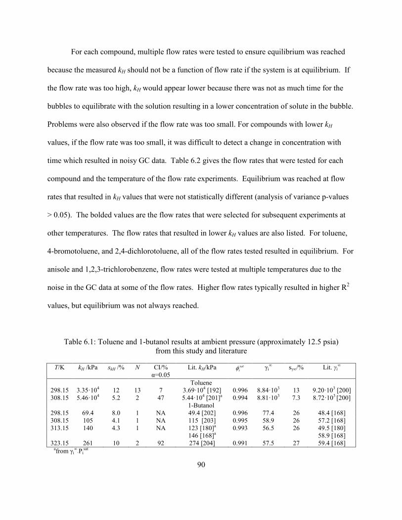
90

For each compound, multiple flow rates were tested to ensure equilibrium was reached

because the measured kH should not be a function of flow rate if the system is at equilibrium. If

the flow rate was too high, kH would appear lower because there was not as much time for the

bubbles to equilibrate with the solution resulting in a lower concentration of solute in the bubble.

Problems were also observed if the flow rate was too small. For compounds with lower kH

values, if the flow rate was too small, it was difficult to detect a change in concentration with

time which resulted in noisy GC data. Table 6.2 gives the flow rates that were tested for each

compound and the temperature of the flow rate experiments. Equilibrium was reached at flow

rates that resulted in kH values that were not statistically different (analysis of variance p-values

> 0.05). The bolded values are the flow rates that were selected for subsequent experiments at

other temperatures. The flow rates that resulted in lower kH values are also listed. For toluene,

4-bromotoluene, and 2,4-dichlorotoluene, all of the flow rates tested resulted in equilibrium. For

anisole and 1,2,3-trichlorobenzene, flow rates were tested at multiple temperatures due to the

noise in the GC data at some of the flow rates. Higher flow rates typically resulted in higher R2

values, but equilibrium was not always reached.

Table 6.1: Toluene and 1-butanol results at ambient pressure (approximately 12.5 psia) from this study and literature

T/K kH /kPa skH /% N CI/% α=0.05

Lit. kH/kPa satiφ γi

∞ sγ∞/% Lit. γi∞

Toluene 298.15 3.35·104 12 13 7 3.69·104 [192] 0.996 8.84·103 13 9.20·103 [200] 308.15 5.46·104 5.2 2 47 5.44·104 [201]a 0.994 8.81·103 7.3 8.72·103 [200]

1-Butanol 298.15 69.4 8.0 1 NA 49.4 [202] 0.996 77.4 26 48.4 [168] 308.15 105 4.1 1 NA 115 [203] 0.995 58.9 26 57.2 [168] 313.15 140 4.3 1 NA 123 [180]a 0.993 56.5 26 49.5 [180]

146 [168]a 58.9 [168] 323.15 261 10 2 92 274 [204] 0.991 57.5 27 59.4 [168]

afrom γi∞

·Pisat

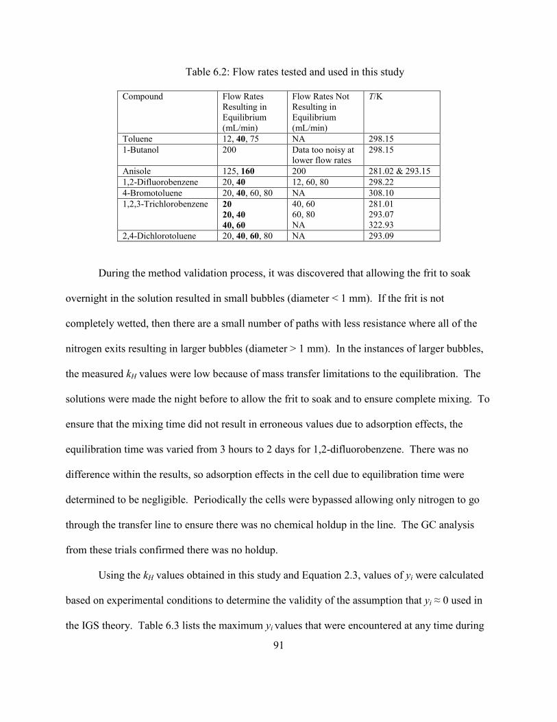
91

Table 6.2: Flow rates tested and used in this study

Compound Flow Rates Resulting in Equilibrium (mL/min)

Flow Rates Not Resulting in Equilibrium (mL/min)

T/K

Toluene 12, 40, 75 NA 298.15 1-Butanol 200 Data too noisy at

lower flow rates 298.15

Anisole 125, 160 200 281.02 & 293.15 1,2-Difluorobenzene 20, 40 12, 60, 80 298.22 4-Bromotoluene 20, 40, 60, 80 NA 308.10 1,2,3-Trichlorobenzene 20

20, 40 40, 60

40, 60 60, 80 NA

281.01 293.07 322.93

2,4-Dichlorotoluene 20, 40, 60, 80 NA 293.09

During the method validation process, it was discovered that allowing the frit to soak

overnight in the solution resulted in small bubbles (diameter < 1 mm). If the frit is not

completely wetted, then there are a small number of paths with less resistance where all of the

nitrogen exits resulting in larger bubbles (diameter > 1 mm). In the instances of larger bubbles,

the measured kH values were low because of mass transfer limitations to the equilibration. The

solutions were made the night before to allow the frit to soak and to ensure complete mixing. To

ensure that the mixing time did not result in erroneous values due to adsorption effects, the

equilibration time was varied from 3 hours to 2 days for 1,2-difluorobenzene. There was no

difference within the results, so adsorption effects in the cell due to equilibration time were

determined to be negligible. Periodically the cells were bypassed allowing only nitrogen to go

through the transfer line to ensure there was no chemical holdup in the line. The GC analysis

from these trials confirmed there was no holdup.

Using the kH values obtained in this study and Equation 2.3, values of yi were calculated

based on experimental conditions to determine the validity of the assumption that yi ≈ 0 used in

the IGS theory. Table 6.3 lists the maximum yi values that were encountered at any time during

92

any of the runs for each compound. The most significant yi is from the 1,2-difluorobenzene

experiments. However, this contribution was still considered negligible. Since the cells were

used for multiple, randomized experiments, the majority of the runs associated with a given

temperature had a much lower initial concentration. There was not a statistically significant

difference between the kH values from the experiment with the starting concentration listed in

Table 6.3 and the experiments that had smaller starting concentrations. The kH values from runs

that started at a more dilute condition were not statistically different from those that started at

higher concentrations.

Table 6.3: Maximum headspace concentrations possible in this study

Compound Max yi (mole fraction) Toluene 3.09∙10-2

1-Butanol 2.86∙10-3 Anisole 1.06∙10-2

1,2-Difluorobenzene 1.08∙10-1 4-Bromotoluene 2.19∙10-3

1,2,3-Trichlorobenzene 1.46∙10-4 2,4-Dichlorotoluene 3.05∙10-3

Solutions of varying concentrations of both 1,2-difluorobenzene and toluene were made

in order to verify the linearity of the detector (FID). A linear response was observed for both

compounds. Peak areas for the vapor samples observed during experimentation fell within the

peak areas of the liquid samples used to check linearity. For the other compounds, it was

assumed that the detector response was linear because small concentrations were used.

During the experiments, it was observed that adsorption effects in the apparatus became

significant after the concentration in the cell dropped below a lower limit. A wide range of kH

93

values were obtained for the same compound at the same temperature and flow rate even though

the plots of ln(A/A0) versus time had R2 values greater than 0.99. Plots were made of the slope

(Equation 5.23) as a function of time to determine how the cumulative slope changed with the

addition of a new point. In some cases, the slope equilibrated to a constant value whereas in

other instances it never settled as illustrated with 1,2-difluorobenzene data in Figure 6.1 and

Figure 6.2. Figure 6.1 shows GC data from two separate experiments at the same conditions.

Both experiments resulted in high R2 values (>0.99); however, they gave different slopes

resulting in significantly different kH values. Figure 6.2 shows the change of slope with time for

the GC data shown in Figure 6.1. The cumulative slope of Run A never settled to a constant

value. In all instances where the slope continued to change with time for each compound, the kH

values were lower than when the slope reached a constant value. The changing slope only

occurred when the peak areas (solute concentration) dropped below a value that was compound

dependent. It is suspected that adsorption effects in the cell became significant once the solution

concentration dropped below a certain value. Since calibration is not required for this method,

the exact lower limit concentrations were not determined. The lower limit was estimated to be

below 1% of the solubility limit with 1,2-difluorobenzene. The plots of the cumulative slope

versus time allowed determination of when this lower limit was passed for each compound. Data

were not used to deter mine kH values from any experiments where adsorption was significant.

94

Figure 6.1: GC data for two separate 1,2-difluorobenzene experiments at 323.15 K and a N2 flow rate of 40 mL/min that resulted in different slopes (a)

Figure 6.2: Cumulative slopes (a) from GC data shown in Figure 6.1 as a function of time

95

The average experimental kH values from this study and corresponding γi∞s are

summarized in Table 6.4 along with satiφ and Ψ values used in the calculations when the solute is

a liquid or solid, respectively. The number of experiments at each temperature, N, and the

standard deviation of the kH average, skH, are included. Also given are the average kH 95%

confidence intervals (CIs) calculated using a Student’s T distribution. The CIs are reported as a

percentage of the average. For some compounds, Bii values were unavailable from the

DIPPR®801 [117] database at the experimental temperatures, so in these cases satiφ was assumed

to be unity. The satiφ values for 1,2-difluorobenzene indicate that this assumption was valid since

the values are close to unity. The reported γi∞ standard deviations, sγ∞, were determined using

the skH values and propagation of error. For compounds where satiφ was assumed to be unity, the

satiφ error was assumed to be 10% in the propagation of error calculations. This is a conservative

error estimation since the 1,2-difluorobenzene values indicate a difference of 1-2% from unity.

In some instances the errors associated with γi∞ are significantly larger than those associated with

kH due to the uncertainty of satiφ or Ψ. Details about each experimental run are included in

Appendix D.

Figure 6.3 shows the 1,2,3-trichlorobenzene kH values obtained in this study along with

those found in the literature. There are many literature values for 1,2,3-trichlorobenzene and

considerable scatter in the literature values. There are also inconsistent temperature trends among

the extant data. The measurements made in this study provide a strong linear trend with small

uncertainty in the temperature dependence. The temperature trend of this study is in good

agreement with the data of reference h [205]. While the temperature-dependent slope of the

values reported by reference c [206] is consistent with the results obtained here, their absolute

96

values appear too high at any given temperature. Much of the other literature data are scattered

about the values reported here but do not provide a clear temperature-dependent trend owing to

the magnitude of that scatter.

Table 6.4: kH and γi∞ values at ambient pressure (approximately 12.5 psia)

from this study and literature

T/K kH/kPa skH/% N CI/%

α = 0.05 Lit. kH/kPa satiφ Ψ γi

∞ sγ∞/%

Anisole

280.95 8.35·102 10 5 12 1a - 5.60·103 14 293.16 1.48·103 4.4 6 4.6 1.48·103[206]b 1a - 4.23·103 11 308.15 2.95·103 5.6 4 8.8 1a - 3.32·103 12 322.90 5.72·103 3.6 5 4.5 1a - 2.83·103 11

1,2-Difluorobenzene

298.19 4.35·104 2.3 4 3.6 3.95·104 [207]c 0.991 - 6.13·103 10 308.12 6.65·104 3.6 3 9.0 0.988 - 5.89·103 11 317.90 9.33·104 2.7 3 6.7 0.984 - 5.41·103 10 322.89 1.05·105 6.4 5 7.9 0.982 - 4.94·103 12

4-Bromotoluene

293.10 1.18·104 1.6 3 4.0 - 0.870 9.04·104 26 298.16 1.71·104 6.0 3 15 1.77·104[208]c - 0.965 9.41·104 26 308.10 2.76·104 5.1 12 3.2 1a - 8.30·104 12 318.03 4.03·104 11 2 95 1a - 6.92·104 15 322.91 5.28·104 2.3 3 5.7 1a - 6.99·104 11

1,2,3-Trichlorobenzene

280.95 3.36·103 8.9 3 22 3.01·103[205]b,d - 0.440 4.34·105 17 293.06 6.84·103 5.0 4 7.9 - 0.535 3.27·105 11 308.14 1.44·104 6.4 5 7.9 - 0.703 2.34·105 8.8 322.99 2.81·104 12 8 10 - 0.946 1.83·105 13

2,4-Dichlorotoluene

280.94 7.14·103 21 4 33 1a - 4.39·105 23 293.09 1.68·104 15 14 8.6 1a - 3.99·105 18 308.15 3.25·104 24 5 30 3.38·104[8]c 1a - 2.66·105 27 323.10 7.54·104 20 4 32 1a - 2.41·105 23 a sat

iφ error of 10% assumed for propagation of error b291.15 K cfrom Pi

sat/xiaq at 298.15 K

d277.15 K

97

Figure 6.3: 1,2,3-Trichlorobenzene kH values from this study and from literature. Values from references marked with an asterisk (*) are xi

aq data converted to kH values using Equation 4.1. References: a [209], b [71], c [206], d* [210], e* [211], f* [212], g* [213], h* [205], i* [207] , j* [214]

Figure 6.4 shows the anisole kH values obtained in this study along with those found in

the literature. The measurements from this study show good agreement with the anisole xiaq data

at higher temperatures and match the directly reported kH values at the lower temperatures. The

kH values obtained from the literature xiaq data are considered to be low in the lower temperature

range. This means that the literature anisole xiaq values at the lower temperatures have higher

errors than the rest of the xiaq data set.

98

Figure 6.4: Anisole kH values from this study and from the literature. Values from references marked with an asterisk (*) are xi

aq data converted to kH values using Equation 4.1. References: a [172], b [206], c* [215], d* [118], e* [216]

The 2,4-dichlorotoluene results are shown in Figure 6.5. The results from this study fall

within the trend of the literature xiaq data. The remaining compounds have very little literature

data available for comparison. Figure 6.6 shows the 1,2-difluorobenzene results from this study

with the single literature xiaq value. The difference between the literature value and the value

from this study at the same temperature could reasonably be due to experimental uncertainty.

The 4-bromotoluene results are shown in Figure 6.7. The data of this study agree the best with

the literature xiaq value.

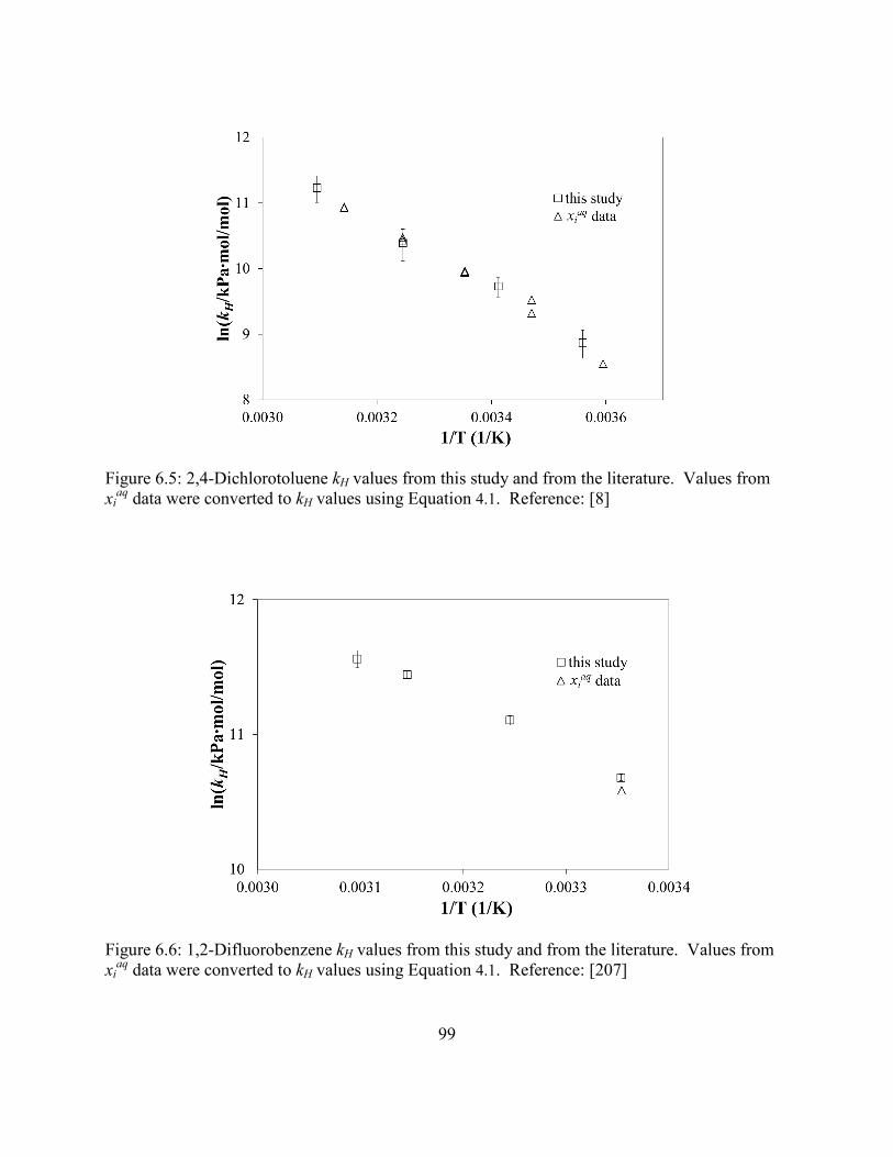
99

Figure 6.5: 2,4-Dichlorotoluene kH values from this study and from the literature. Values from xi

aq data were converted to kH values using Equation 4.1. Reference: [8]

Figure 6.6: 1,2-Difluorobenzene kH values from this study and from the literature. Values from xi

aq data were converted to kH values using Equation 4.1. Reference: [207]

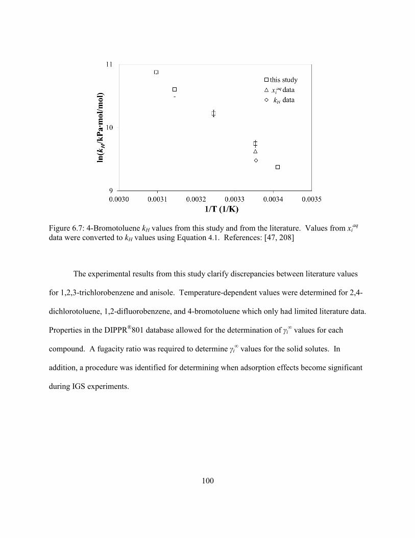
100

Figure 6.7: 4-Bromotoluene kH values from this study and from the literature. Values from xiaq

data were converted to kH values using Equation 4.1. References: [47, 208]

The experimental results from this study clarify discrepancies between literature values

for 1,2,3-trichlorobenzene and anisole. Temperature-dependent values were determined for 2,4-

dichlorotoluene, 1,2-difluorobenzene, and 4-bromotoluene which only had limited literature data.

Properties in the DIPPR®801 database allowed for the determination of γi∞ values for each

compound. A fugacity ratio was required to determine γi∞ values for the solid solutes. In

addition, a procedure was identified for determining when adsorption effects become significant

during IGS experiments.

101

7 Prediction Methods

7.1 Overview of Prediction Method Types

This section provides general information about the types of prediction methods available

in the literature. Property-property relationships (PPRs) relate the property of interest to other

properties of the chemical [24]. These relationships can be thermodynamically based or strictly

empirical. PPRs are often restricted to the chemical classes from which they were derived [217].

Group-contribution methods (GCMs) parse the chemical’s structural formula into

functional groups and fragments, and the property of a compound is estimated by summing

together the contributions of each segment [218]. First-order methods use groups that do not

take into account interactions with neighboring compounds. Second-order methods are more

complex because neighboring atoms are included in the group definitions. Limitations of these

methods are their inability to differentiate between isomers and large errors for compounds with

multiple non-alkyl functional groups. Empirical corrections are often used to offset these

deviations. Group-contribution methods fail when a compound contains a functional group that

was not contained in the original training set of the method [14, 219]. Bond contribution

methods (BCMs) work in a similar fashion; they add up the contributions from each bond in the

molecule.

Quantitative structure-property relationships (QSPRs) are based on fragment

contributions and structural descriptors [24]. Descriptors (such as topological indices, molecular

102

volume, molecular surface area, etc.) are calculated from molecular structure [220]. There are

various software tools and methods for obtaining and selecting descriptors with some being more

complex than others. Another name associated with methods of this type is quantitative

structure-activity relationships (QSARs).

Linear Solvation Energy Relationships (LSERs) relate the Gibbs energy of solution of a

solute to a series of empirical parameters that describe the cavity formation and the solute-

solvent interaction processes that occur when a gaseous solute dissolves in a liquid [221].

LSERs are a type of QSPR [222]. Parameters used (often called “solvatochromic parameters”)

include solute dipolarity/polarizability, hydrogen bond donor acidity, and hydrogen bond

acceptor basicity. These parameters originate from experimental data which are not always

available for every compound.

Molecular simulations (such as Monte Carlo) and quantum mechanical methods (such as

continuum-solvation models) have high computational costs making them difficult to use for

predicting properties of large groups of compounds [219, 223]. A continuum-solvation model

(CSM) that has become more prominent is the Conductor-like Screening Model for Real

Solvents (COSMO-RS). COSMO-RS is a surface interaction model that uses molecular charge

densities obtained by molecular quantum chemical calculations [224, 225]. An advantage of

COSMO-RS is that only a few adjustable parameters are required [226].

Neural networks (NN) have become more popular in prediction method development.

Neural networks consist of many processing units arranged in a network [227]. The networks

have an input layer, an output layer, and intermediate hidden layers. Each network unit is

influenced by connected units, and the extent of influence can be changed by adjusting the

weights of the connections. Learning algorithms are used to modify the system behavior by

103

changing the values of these weights. While these methods have been shown to perform well,

they are impossible to duplicate from literature articles. The model would have to be obtained

from the author in order to use the method.

7.2 Prediction Method Selection

Most kH prediction methods only predict values at 298.15 K. Table 7.1 lists some of the

available prediction methods for kH at 298.15 K. UNIFAC expansions were excluded from the

table due to the large number of authors that have added to this method. Dearden and

Schüürmann [14] compared 12 of these methods and found that the EPA’s HENRYWIN bond

contribution method [83] outperformed the other methods. Values predicted from this method

have been included as constant value entries in the database. The actual method was not

programmed into DIADEM because it uses hundreds of bond contributions. The software is

available without cost from the EPA website. The predicted values were imported into the

database from the software.

There are significantly fewer kH methods that predict temperature dependence, and it was

determined that the greatest contribution can be made to these methods. An initial review was

conducted on temperature-dependent prediction methods to determine the methods to include in

this study. Temperature-dependent prediction methods that were excluded are listed in Table 7.2

with a brief reason for exclusion. The method of Yezdimer, Sedlbauer, and Wood (2000) [276]

applies to some chemical families that were not included in the database analysis. Of the groups

that applied to compounds included in this study, a similar method was published a few years

later with superior contributions (see Section 7.2.1). The methods of Goss [277] and Abraham et

al. [278] both require molecular descriptors that are based on experimental data. These methods

104

were excluded due to the time that would be required to find reported descriptor values in the

literature for the compounds in the database. The method of Hilal et al. [279, 280] uses two

independent models to predict xiaq and Pi

sat and then calculates kH using Equation 4.1. There are

publications concerning the method performance, but no publications have been found on the

actual method parameters preventing the inclusion of this method in this study.

Table 7.1: kH prediction methods at 298.15 K

Authors Method Type

Authors Method Type

Authors Method Type

Hine and Mookerjee (1975) [23, 228]

(1) BCM (2) GCM

Cramer and Truhlar (1992) [262]

CSM Dearden et al. (2000) [249]

QSPR

Cramer (1980) [230] QSPR Jorgensen and Nguyen [263] (1993)

Monte Carlo

Meylan and Howard (2000) [219]

(1) BC & (2) GC

Cabani (1981) [232] GCM Myrdal (1994) [265] PPR Öberg (2001) [252] QSPR Shiu and Mackay (1986) [234]

PPR Abraham et al. (1994) [267] LSER Ferreira (2001) [254] QSPR

Jin et al. (1986) [236] GCM Schüürmann (1995) [269] CSM Yao et al. (2002) [256] QSPR Nirmalakhandan and Speece (1988) [238]

QSPR Chambers et al. (1996) [271] CSM Lin and Sandler (2002) [218]

GCM

Hawker (1989) [23, 240]

QSPR Dearden et al. (1997) [272] QSPR Yaffe et al. (2003) [259]

QSPR with NN

Sabljic and Gusten (1989) [23, 242]

QSPR Schüürmann (1997) [274] software

Modarresi et al. (2005) [261]

QSPR

Brunner et al. (1990) [23, 248]

QSPR Barone et al. (1997) [229] CSM Modarresi et al. (2007) [219]

QSPR

Crovetto et al. (1990) [250]

PPR Hawkins et al. (1997) [231] CSM Schröder et al. (2010)[264]

COSMO-RS

Meylan and Howard (1991) [251]

BCM Hawkins et al. (1998) [233] CSM Gharagheizi et al. (2010) [266]

GCM with NN

Yaws et al. (1991) [13], (2010) [253]

Must be bought

Katritzky et al. (1998) [235] QSPR Goodarzi et al. [268] QSPR with NN

Suzuki et al. (1992) [255]

GCM & QSPR

Famini et al. (1999) 32 [237] LSER Peterson (2011) [270] QSPR

Russell et al. (1992) [257]

QSPR Cash (1999) [239] QSPR Gharagheizi et al. (2010) [266]

GCM with NN

Dunnivant et al. (1992) [258]

QSPR Gramatica et al. (1999) [241] QSPR with NN

Raventos-Duran (2010) [273]

GCM

Cramer and Truhlar 36 [260](1992)

CSM Plyasunov and Shock (2000) [243] (2004) [244] (2005) [245] (2006) [246, 247]

GCM Sahoo (2011) [275] QSPR

105

Table 7.2: kH temperature-dependent prediction methods excluded from this study

Author Method Description Reason for Exclusion Yezdimer, Sedlbauer, and Wood (2000) [276]

GCM; need water equation of state

Similar, superior method published later

Goss (2006) [277] LSER Difficulty in obtaining descriptors Abraham et al. (2007) [278]

LSER Difficulty in obtaining descriptors

Nirmalakhandan et al. (1997) [281]

QSPR Does not apply to very many compounds

Huang et al. (2009) [282]

Molecular Simulation Computational cost and difficulty obtaining models

Hilal et al. (2008) [279, 280]

SPARC-solvation model Publications on method performance but not method parameters

Table 7.3 lists the temperature-dependent prediction methods that have been programmed

into DIADEM along with the type of method and the applicable compounds. The GCM and

BCM methods developed by Lau et al. [39] are applicable for different chemical families. The

chemical families that do not overlap between the methods are italicized. Initially the plan was

to add to one of these existing methods. However, it was decided to develop a completely

different method. The methods listed in Table 7.3 are described in more detail along with

reasons they were not expanded in this study. A quantitative comparison of the methods is

provided in Section 7.2.5.

Table 7.3: kH temperature-dependent prediction methods chosen for evaluation

Author Method Description Applicable compounds Sedlbauer et al. (2002) [191], (2007) [283] and (2008) [22]

GCM; need water equation of state

alkanes, alkenes, alkyl phenols, alkyl anilines, aromatic hydrocarbons, cycloalkanes, H2S, and CO2

Plyasunov and Shock (2003) [284]

GCM substructural parameters with atom types C, H, N, O, F, Cl, Br, I, and S

Kühne, Ebert, and Schüürmann (2005) [285]

GCM & BCM; need a reference value

substructural parameters with atom types C, H, N, O, F, Cl, Br, I, and S

Lau, Rogers, and Zei (2010) [39]

Separate GCM & BCM; need a reference value

GCM: alkanes, cycloalkanes, cycloalkenes, alkylbenzenes, primary alcohols, secondary alcohols, aliphatic chlorides, ketones

BCM: alkanes, alkenes, cycloalkanes, alkylbenzenes, aliphatic chlorides, ketones

106

7.2.1 Method of Sedlbauer et al. [22, 191, 283]

This method was initially published for aqueous hydrocarbons by Sedlbauer, Bergin, and

Majer in 2002 [191]. In 2008, the same authors published additional parameters for CH4, CO2

and H2S [22]. Parameters for alkylphenols and alkylanilines were developed in 2007 by Čenský,

Sedlbauer, Majer, and Růžička [283] using the hydrocarbon parameters developed in 2002.

Because these parameters can all be used together, they have been lumped together as one

method even though the parameters were published in three separate papers.

In addition to predicting kH, this method also predicts models for derivative properties

(Equations 2.4-2.7). Experimental data related to the derivative properties were used in addition

to kH, xiaq, and γi

∞ data to develop this prediction method. The experimental data were

simultaneously fit to a semitheoretical hydration model that uses the derivative property

relationships. Group contribution values are used to calculate a reference value at Tref and Pref

(298.15 K and 0.1 MPa), and a separate set of group contribution values are used to model the

temperature and pressure dependency. The Plyasunov and Shock [243] group contribution

values at reference conditions were used for hydrocarbons. The hydration model requires

properties of water that can be calculated using an equation of state. Sedlbauer et al. [22, 191,

283] used the equation of state by Hill [286]. The IAPWS-95 [287] equation of state was used

when programming this method into DIADEM. This difference should not affect method

performance.

This method applies to hydrocarbons up to temperatures and pressures of approximately

570 K and 100 MPa, respectively. This broad range allows the prediction method to be

applicable for systems encountered in the oil and natural gas industries. Since this method is

both a function of temperature and pressure and DIADEM allows for one dependent variable, the

107

variable of pressure was “removed” by using the DIPPR® 801 liquid density equation for water

(which only has the dependent variable of temperature) in all calculations that required density.

This results in thermodynamic properties of water along the saturation line.

This method was not chosen for expansion in this study because derivative properties

were not included in the database. In addition, this model extends beyond the temperature and

pressure scope of the data evaluated in this study.

7.2.2 Method of Plyasunov and Shock [284]

The method of Plyasunov and Shock [284] is a group contribution method that predicts

values of the vapor-liquid distribution coefficient (KD) from 273 K to the critical temperature of

water (647.1 K). KD, is related to kH by:

satsolviDH PKk ∞= φ ,

where ϕi∞ is the fugacity coefficient of the solute at infinite dilution and sat

solvP is the vapor

pressure of water. The method includes group contribution values of ϕi∞ allowing for kH to be

calculated. High-temperature calculations are based on the Krichevskii parameter. This method

uses water vapor pressure, and liquid and vapor water densities obtained from the IAPWS-95

equation of state [287]. This model was developed for hydrothermal geochemical applications

which are interested in high-temperature and high-pressure values.

The Plyasunov and Shock method [284] was not the most accurate of the prediction

methods evaluated in this study which is possibly due to the target temperature range of

applicability. This method may be more accurate at near-critical conditions compared to

methods that were developed using data closer to ambient conditions. However, the prediction

108

capabilities of this method at high temperatures and pressures were not determined because these

conditions are beyond the scope of the data evaluated in this study. This method was not chosen

for additional development or refinement due to the temperature scope of data included in this

project. In addition, any development of this method would require Krichevskii parameters

which were not included in the database.

7.2.3 Methods of Lau et al. [39]

Lau et al. [39] published separate bond and group contribution methods in the same

paper. From a statistical standpoint, these methods are equivalent in their prediction capabilities.

There are differences in the chemical families covered by both methods as indicated in Table 7.3.

The chemical families that do not overlap between the methods are italicized. Temperature

dependence is modeled using a variation of DIPPR® 801 Equation 101 (see Table 4.3),

+

−

=

∑∑

refiii

refiii

refH

H

TTnC

TTnB

kk ln11ln

,

, 7.1

where Bi and Ci are group contribution values for fragment i, ni is the number of times a group

occurs, T is temperature, and superscript ref refers to a reference value obtained from

experimental data or a prediction method. Since ln(kH) is related to ∞∆ hydG (Equation 2.4),

coefficients “B” and “C” are related to ∞∆ hydH (through integration of Equation 2.5) and ∞∆ hydCp

(through integration of Equation 2.6), respectively. Both the bond and group contribution

methods predict coefficients “B” and “C” given in Equation 7.1. This method was not chosen for

expansion in this study due to the requirement of a reference value. In addition, some of the

109

group (and/or bond) contributions were developed on limited data. More data for similar

compounds are available in the 801E database.

7.2.4 Method of Kühne, Ebert, and Schüürmann [285]

The method of Kühne et al. [285] predicts temperature-dependence using an abbreviated

form of Equation 7.1. This method uses group contribution values and correction factors to

predict coefficient “B”, so it only predicts a linear relationship between ln(kH) and inverse

temperature. Therefore, it can only be applied over a more limited range of temperature than the

method of Lau et al. [39]. Out of the temperature-dependent methods programmed into

DIADEM, this method has the widest chemical family applicability. This method was not

chosen for expansion due to its limited temperature applicability and the requirement of a

reference value.

7.2.5 Existing Method Comparison

The prediction methods were compared using data for 157 compounds. Some of the

methods apply to compounds outside of the chemical families included in the comparison. Only

the compounds included in later method development were included to make the comparisons

more meaningful. The number of applicable compounds (nC) and the average absolute

deviations (AAD) for each chemical family and method are summarized in Table 7.4. Also

included is a breakdown of the AAD based on the error of the experimental data.

The methods of Plyasunov and Shock [284] and Kühne et al. [285] apply to all of the

compounds included in the comparison, but the method of Kühne et al. [285] has a smaller

overall AAD. The Lau et al. [39] methods have comparable overall performances, but the group-

110

contribution method applies to more of the compounds included in the comparison. The Lau et

al. [39] methods are better than the Kühne et al. [285] method, and this can be attributed to the

additional temperature-dependent coefficient. The Sedlbauer et al. [22, 191, 283] method applies

to the smallest group of compounds. It does not perform as well as the Lau et al. [39] methods.

However, the Lau et al. [39] methods use an experimental reference value whereas the Sedlbauer

et al. [22, 191, 283] method is completely predictive.

7.3 Prediction Method Development

While the Kühne et al. [285] and Lau et al. [39] methods have reasonable prediction

capabilities, they both require a reference value. The reference value can be an experimental

value or it can predicted using a separate prediction method. Prediction methods that can be

used to calculate a reference value are not available that use the same group definitions as Kühne

et al. [285] or Lau et al. [39]. It was decided that a prediction method would be developed that

uses the same group definitions for all parameters including the reference value. This simplifies

the calculations because each compound only has to be parsed once.

Initially efforts were made to develop a group contribution method that predicted

coefficients “A”, “B”, and “C” of DIPPR® Equation 101 simultaneously. This did not work well

due to the high number of parameters. Instead, it was decided to use the method of Plyasunov et

al. [243] for the reference values, and then develop a model using the same group definitions to

predict coefficients “B” and “C” in Equation 7.1. Sedlbauer et al. [191] uses the method of

Plyasunov et al. [243] as a reference point in their prediction method. Plyasunov et al. [243] did

a thorough literature review of kH and derivative property data for hydrocarbons. They provided

recommended values for each compound and developed their prediction methods based on these

111

values. While this method is more limited in chemical applicability than the HENRYWIN bond-

contribution method [83], the method is more reliable due to the data used for method

development.

Table 7.4 Temperature-dependent kH prediction method comparison for select compounds

Method Plyasunov and Shock

AAD% nC Kühne nC

Lau GCM

AAD% nC

Lau BCM

AAD% Comps Sedlbauer

AAD% nC

Overall 139.8 157 40.4 157 16.9 98 13.8 69 30.1 46 Acetates 71.8 14 15.2 14 - - - - - -

Aliphatic ethers 176.8 11 18.6 11 - - - - - - Dimethylalkanes 87.4 6 113.8 6 12.7 6 12.6 6 65.7 6

Formates 84.3 7 14.9 7 - - - - - - Ketones 91.9 24 34.6 24 39.5 21 23.6 22 - -

Methylalkanes 43.9 8 18.3 8 3.9 8 4.0 8 20.8 8 n-alcohols 62.9 10 29.7 10 14.5 10 - - - - n -alkanes 64.3 14 102.6 14 11.9 14 12.2 14 32.1 14

n -alkylbenzenes 139.2 8 18.5 8 7.8 8 7.7 8 19.0 8 Other aliphatic

alcohols 87.9 21 20.5 21 11.5 21 - - - -

Other alkanes 82.0 2 14.8 2 11.2 2 2.7 2 24.2 2 Other

alkylbenzenes 949.3 9 145.0 9 10.5 8 10.1 9 22.0 8

Other ethers/diethers 92.3 5 10.9 5 - - - - - -

Other polyfunctional C,

H, O 97.9 2 10.6 2 - - - - - -

Other saturated aliphatic esters 84.0 3 31.0 3 - - - - - -

Propionates and butyrates 93.6 13 26.4 13 - - - - - -

< 1% 81.1 1 11.6 1 2.1 1 4.7 1 24.2 1 < 3% 74.2 11 11.9 11 4.5 8 4.3 7 11.3 7 < 5% 112.3 27 23.8 27 6.3 19 6.0 12 14.9 9

< 10% 119.0 77 36.2 77 10.4 52 8.4 34 21.1 19

< 25% 124.0 71 51.8 71 33.7 43 28.5 28 41.0 16

< 50% 161.8 34 49.7 34 36.5 27 35.0 19 48.1 15 < 100% 513.8 15 65.3 15 76.2 9 75.4 8 77.5 6

112

Initially Plyasunov et al. [243] developed a first-order group contribution prediction

method for hydrocarbons and alcohols. Additional functional group contribution terms were

added to their method in later publications [245-247, 288]. In these later publications, second-

order group contribution parameters were also developed. However, second-order hydrocarbon

groups were not defined for all of the hydrocarbons included in the original first-order method.

In this study, both the first- and second-order methods were expanded.

The method of Plyasunov et al. [243] uses the relationship between kH and ∞∆ hydG

(Equation 2.4). Plyasunov et al. [243] define the standard state in terms of molality (standard

molality of 1 mol/1000 g at a Pref of 100 kPa), so a unit conversion must be used with the

definition of kH in this study,

∞∆=

⋅ hydWref

H GNP

kRT ln , 7.2

where NW = (1000 g/1 mol)/(18.0153 g/mol) ≈ 55.5084 (mol/mol). The group contribution

values determined by Plyasunov et al. [243] are given in terms of ∞∆ hydG . For the first- and

second-order methods of this study, values for kH,ref are calculated using Equation 7.2. Using a

group contribution scheme, any property (Y) can be determined by:

∑+=i

iiYnYY 0 7.3

where ni is the number of a times group i appears in the compound, Yi is the contribution of the

group to the overall property, and Y0 is a constant. Plyasunov and Shock [243] defined a Y0

value of 7.95 kJ/mol for ∞∆ hydG based on theoretical models (the contribution of a material

point). The Y0 values for B and C are 0 for the first- and second-order methods of this study.

113

7.3.1 Data Selection

The first step was selecting the data to use in method development. The recommended

values at 298.15 K of this study were used in constant value (or reference value) method

development. With temperature-dependent models, there are multiple ways that data are used.

1. Regression coefficients are determined from the data, and the prediction method is then

developed from the regression coefficients (A, B, C, etc.) and not directly from data.

Examples are the methods of Kühne et al. [285], Nagvekar [289], Hsu [290].

2. Regression coefficients are determined from the data, and values are calculated at equal

temperature intervals (such as every 10 K) using the regression. The prediction method

is developed from these values. Examples include prediction methods developed by Elbro

et al. [291] and Harrison [292].

3. Prediction method is developed directly from data.

The first two options were not used due to the different temperature ranges of available

data. The coefficients obtained in the data analysis of this study do not refer to the same

temperature ranges. In addition, a second temperature-dependent coefficient is not statistically

significant for some compounds due to the limited data. A combination of Options 2 and 3 was

determined to be the best method. The data were not used directly due to the extreme

distribution of the number of points per compound in addition to the experimental error. For

example, benzene has 341 experimental points whereas 1,2,3,4-tetramethylbenzene has 3

experimental points. Smoothed values were calculated from the regressions obtained in the data

analysis process at every unique temperature found within the data of a given compound. For

example, if data are available for a compound at temperatures of 275 K, 298 K, 298 K, and 330

K, values calculated from the regression at 275 K, 298 K, and 330 K were included in the

114

method development. The uncertainties assigned to the regression (determined from 95%

confidence intervals during data analysis) were then assigned to these smoothed points.

Compounds with more temperature-dependent data will also inherently have more weight due to

the existence of more unique temperatures.

A similar process was used for the data of compounds in which the API regression was

accepted (see Section 4.5). The unique temperatures of the data in the 801E database were

determined for a given compound. The Smoothed values were determined using the API

regressions.

A weighted least-squares procedure was used to determine the group contribution values.

The objective function, O, to be minimized is defined by

2exp,mod, lnln∑

−=

i i

iH

iH kkO

σ, 7.4

where lnkHmod,i are the natural log values calculated from the model, lnkH

exp,i are the natural log

experimental values, and σi is the uncertainty (on a natural log scale) of the Smoothed value. By

using weighted values, Smoothed values with smaller uncertainty will be given greater weight in

the regression. In this study, the weighted least-squares procedure was completed using SAS®

software.

7.3.2 Validation Techniques

A general procedure was used multiple times throughout method development.

Approximately 10% of the compounds were assigned to a validation set. The remaining

compounds (training set) were then randomly divided into 10 subsets to perform a 10-fold cross-

validation. In the 10-fold cross-validations, a single subset of the training set was reserved as a

115

prediction set and the remaining 9 were used as a learning set. A preliminary model was

developed using the learning set and applied to the prediction set. This process was repeated so

that each subset was used as the prediction set once. The statistics from the 10 iterations were

averaged to provide a better estimation of the overall method accuracy. The entire training set

was then used to develop model parameters. The model was finally applied to the validation set

as an additional check on the method performance.

The average absolute deviation (AAD) is given by:

∑=

−=

n

ii

H

iH

iH

kkk

AAD1

exp,

exp,mod,

. 7.5

The AAD is calculated on a normal scale and not a log scale to provide better insight of the

method performance. Also reported is the Pearson’s product moment correlation coefficient, R2,

(the R2 value returned by the Microsoft Excel® RSQ function) given by

∑∑

∑

−−

−−=

n

i

avgH

iH

n

i

avgH

iH

n

i

avgH

iH

avgH

iH

kkkk

kkkkR

2exp,exp,2mod,mod,

exp,exp,mod,mod,

2

)ln(ln)ln(ln

)ln)(lnln(ln,

7.6

where lnkHexp,avg is the average natural log experimental value used in the training set (or learning

set during cross-validation) and lnkHmod,avg is the average natural log model value used in the

validation set (or prediction set during cross-validation). A reliable method will have R2 values

that approach unity and low AADs for both the training and validation sets.

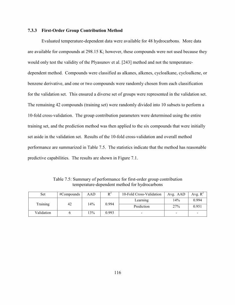
116

7.3.3 First-Order Group Contribution Method

Evaluated temperature-dependent data were available for 48 hydrocarbons. More data

are available for compounds at 298.15 K; however, these compounds were not used because they

would only test the validity of the Plyasunov et al. [243] method and not the temperature-

dependent method. Compounds were classified as alkanes, alkenes, cycloalkane, cycloalkene, or

benzene derivative, and one or two compounds were randomly chosen from each classification

for the validation set. This ensured a diverse set of groups were represented in the validation set.

The remaining 42 compounds (training set) were randomly divided into 10 subsets to perform a

10-fold cross-validation. The group contribution parameters were determined using the entire

training set, and the prediction method was then applied to the six compounds that were initially

set aside in the validation set. Results of the 10-fold cross-validation and overall method

performance are summarized in Table 7.5. The statistics indicate that the method has reasonable

predictive capabilities. The results are shown in Figure 7.1.

Table 7.5: Summary of performance for first-order group contribution temperature-dependent method for hydrocarbons

Set #Compounds AAD R2 10-Fold Cross-Validation Avg. AAD Avg. R2

Training 42 14% 0.994 Learning 14% 0.994

Prediction 27% 0.951 Validation 6 13% 0.993 - - -

117

Figure 7.1: Plot of experimental versus model values for the first-order temperature-dependent group contribution method for hydrocarbons

The compound with the biggest discrepancy in the validation set is 1,4-cyclohexadiene.

It is the only cycloalkene with more than one double bond. (It randomly ended up in the

validation group instead of the training group.) The cyclic compounds also have the largest error

in the training set. There are less data for these compounds and more uncertainty in the available

data compared to the alkanes and benzene derivatives.

The method was expanded for aliphatic alcohols, ketones, and formates. Data were

found for 61 compounds. Seven compounds were randomly chosen for the validation set. The

remaining 54 training set compounds were divided into 10 subgroups. A 10-fold cross validation

118

was performed as previously described. The group contribution parameters were then

determined using the entire training set, and the prediction method was then applied to the seven

compounds in the validation set. Results of the 10-fold cross-validation and overall method

performance are summarized in Table 7.6. The results are shown in Figure 7.2.

Table 7.6: Summary of performance for first-order group contribution temperature-dependent method for alcohols, ketones, and formates

Set #Compounds AAD R2 10-Fold Cross-Validation Avg. AAD Avg. R2

Training 54 24% 0.920 Learning 24% 0.921

Prediction 29% 0.934 Validation 7 33% 0.969 - - -

The two compounds with the largest discrepancies are acetophenone and acetylacetone.

Acetophenone is the only aromatic ketone included in the entire dataset, and acetylacetone is the

only di-ketone included in the entire dataset. The large errors could be attributed to experimental

error and/or the structures. More data from similar compounds would be necessary to determine

the exact cause. The statistics given in Table 7.6 include the results of these two compounds. It

is recommended that this method should only be used for alcohols, ketones, and formates that are

aliphatic. In addition, correction factors might be necessary for multifunctional compounds.

119

Figure 7.2: Plot of experimental versus model values for the first-order temperature-dependent group contribution method for alcohols, ketones, and formates

The temperature-dependent coefficients determined in this study are summarized in

Table 7.7 along with the standard errors and two-tailed p-values. The table also includes the

reference values developed by Plyasunov et al. [243-247], the number of compounds that

contained a group (nC), the total number of temperature-dependent points that contained a group

(nG), and the temperature range of the data used for the individual groups. Multiple coefficients

have large standard errors and are not statistically significant (p-values > 0.05). In general, the

groups corresponding to these coefficients do not have as much data compared to the groups

with statistically significant coefficients resulting in higher uncertainty. When Plyasunov et al.

initially developed the group contribution value for ketones, they did not include a correction

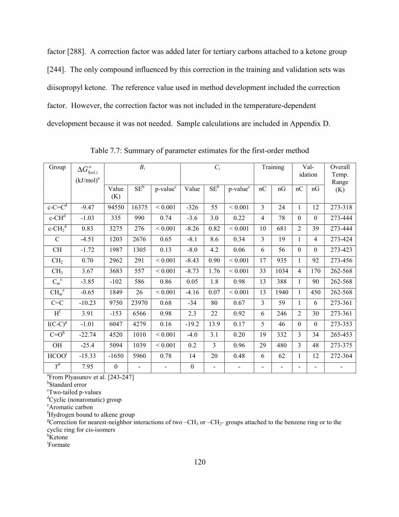
120

factor [288]. A correction factor was added later for tertiary carbons attached to a ketone group

[244]. The only compound influenced by this correction in the training and validation sets was

diisopropyl ketone. The reference value used in method development included the correction

factor. However, the correction factor was not included in the temperature-dependent

development because it was not needed. Sample calculations are included in Appendix D.

Table 7.7: Summary of parameter estimates for the first-order method

Group ∞∆ ihydG , (kJ/mol)a

Bi Ci Training Val-idation

Overall Temp. Range

(K) Value (K)

SEb p-valuec Value SEb p-valuec nC

nG

nC

nG

c-C=Cd -9.47 94550 16375 < 0.001 -326 55 < 0.001 3 24 1 12 273-318 c-CHd -1.03 335 990 0.74 -3.6 3.0 0.22 4 78 0 0 273-444 c-CH2

d 0.83 3275 276 < 0.001 -8.26 0.82 < 0.001 10 681 2 39 273-444 C -4.51 1203 2676 0.65 -8.1 8.6 0.34 3 19 1 4 273-424

CH -1.72 1987 1305 0.13 -8.0 4.2 0.06 6 56 0 0 273-423 CH2 0.70 2962 291 < 0.001 -8.43 0.90 < 0.001 17 935 1 92 273-456 CH3 3.67 3683 557 < 0.001 -8.73 1.76 < 0.001 33 1034 4 170 262-568 Car

e -3.85 -102 586 0.86 0.05 1.8 0.98 13 388 1 90 262-568 CHar

e -0.65 1849 26 < 0.001 -4.16 0.07 < 0.001 13 1940 1 450 262-568 C=C -10.23 9750 23970 0.68 -34 80 0.67 3 59 1 6 273-361 Hf 3.91 -153 6566 0.98 2.3 22 0.92 6 246 2 30 273-361

I(C-C)g -1.01 6047 4279 0.16 -19.2 13.9 0.17 5 46 0 0 273-353 C=Oh -22.74 4520 1010 < 0.001 -4.0 3.1 0.20 19 332 3 34 265-453 OH -25.4 5094 1039 < 0.001 0.2 3 0.96 29 480 3 48 273-375

HCOOi -15.33 -1650 5960 0.78 14 20 0.48 6 62 1 12 272-364 Y0 7.95 0 - - 0 - - - - - - -

aFrom Plyasunov et al. [243-247] bStandard error cTwo-tailed p-values

dCyclic (nonaromatic) group eAromatic carbon fHydrogen bound to alkene group gCorrection for nearest-neighbor interactions of two –CH3 or –CH2- groups attached to the benzene ring or to the cyclic ring for cis-isomers hKetone iFormate

121

Efforts to expand the model to include esters and ethers were unsuccessful because the

first-order contributions were not always adequate in modeling the behavior of compounds with

functional groups [244-247]. Due to these limitations, a different model was pursued.

7.3.4 Second-Order Group Contribution Method

Plyasunov et al. [244-247] developed a second-order group contribution model due to the

first-order limitations. A second-order method takes into account the nearest neighbor

interactions for particular groups. This requires defining more groups than a first-order group

contribution method. The group definitions as outlined by Domalski et al. [293] were used for

parsing the compounds. Plyasunov et al. [244-247] only define four hydrocarbon second-order

contributions. Additional hydrocarbon contributions were first established at 298.15 K before

developing temperature-dependent contributions.

7.3.4.1 Reference Value Additions

The values of the four hydrocarbon groups defined by Plyasunov et al. [244-247] were

used without modification. Values for four alkylbenzene groups were developed in this study.

Accepted kH values at 298.15 K were found for 17 alkylbenzenes. Two of these compounds

were randomly chosen for the validation set. The 15 training set compounds were divided into

10 subgroups. A 10-fold cross validation was performed as previously described. Only three of

the four parameters could be determined in one of the iterations due to the learning model not

being full rank. Of the remaining 9 iterations, the relative absolute standard deviation of the

group contribution values did not exceed 5.6%. Overall parameters were determined using the

full training set, and the model was applied to the validation set. The AAD of the overall

training set was 18% and the AAD of the validation set was 14%.

122

An additional ether term was also developed, C-(H)3(O), for a reference value at 298.15

K. A total of 7 compounds were found with this group. One of the compounds was randomly

set aside for validation. A leave-one-out cross-validation was performed on the remaining 6

compounds (similar idea as the 10-fold cross-validation except each compound is a subset). The

value of the group contribution did not change significantly during cross-validation (standard

deviation of 2%). The AAD of the overall training set (6 compounds) was 21% and the AAD of

the validation set (1 compound) was 1%. Table 7.8 is a summary of the second-order group

contribution values for the prediction method at 298.15 K that were determined in this study and

by Plyasunov et al. [244-247]. The table includes the number of compounds with each group

(nC) and the number of times each group appeared in a set (nG).

7.3.4.2 Temperature-Dependent Contributions

A total of 31 (aliphatic and aromatic) hydrocarbons defined by the groups in Table 7.8

have temperature-dependent data. Four were randomly selected by subfamily (2 alkanes, 2

benzene derivatives) for validation. The training set of 27 compounds was divided into 10

groups for 10-fold cross-validation. Overall parameters were determined using the full training

set. Results of the 10-fold cross-validation and overall method performance are summarized in

Table 7.9 and shown in Figure 7.3.

123

Table 7.8: Summary of second-order group contributions for reference values at 298.15 K and 0.1 MPa

Training Validation ∞∆ ihydG , Groupa nCb nGc nCb nGc kJ/mol SEd p-valuee C-(H)2(C)(Cb) 6 6 0 0 1.02 0.31 0.007 C-(H)3(Cb) 8 21 1 3 4.00 0.33 < 0.0001 Cb-(C)(Cb)2 15 28 1 3 -4.53 0.36 < 0.0001 Cb-(H)(Cb)2 15 62 2 9 -0.60 0.04 < 0.0001 C-(H)3(O) 6 7 1 1 3.48 0.11 < 0.0001 C-(H)3(C)f 7 8 0 0 3.72 - - C-(H)2(C)2

f 5 18 0 0 0.68 - - C-(H)(C)3

f 1 1 0 0 -1.93 - - C-(C)4

f 0 0 0 0 -4.60 - - [CH3-CH2-O-CH2] corrf,g - - - - -1.42 - - [O-(CH2)2-O] corrf,g - - - - 2.22 - - C-(C)(H)2(O)f - - - - 0.77 - - C-(C)2(H)(O) alcoholf - - - - -1.64 - - C-(C)2(H)(O) esterf - - - - -1.46 - - C-(C)2(H)(O) etherf - - - - -2.82 - - C-(C)3(O) alcoholf - - - - -4.58 - - C-(C)3(O) esterf - - - - -2.58 - - C-(C)3(O) etherf - - - - -7.77 - - C-(CO)(C)3

f - - - - -2.50 - - C-(CO)(H)(C)2

f - - - - -0.88 - - C-(CO)(H)2(C)f - - - - 1.15 - - CO-(C)2

f - - - - -23.46 - - COO-(C)2

f - - - - -20.53 - - HCOO-(C)f - - - - -15.43 - - O-(C)(H)f - - - - -25.46 - - O-(C)2

f - - - - -15.52 - - Y0 f - - - - 7.95 - -

aCb is an aromatic carbon (benzene) bnC is the number of compounds with the group cnG is the number of times the group appeared in the set dStandard error eTwo-tailed p-value fDetermined by Plyasunov et al. [244-247] gether corrections; used in addition to group contributions

124

Table 7.9: Performance summary of the second-order temperature-dependent group contribution method for alkylbenzenes

Set #Compounds AAD R2 10-Fold Cross-Validation Avg. AAD Avg. R2

Training 27 10% 0.998 Learning 10% 0.998

Prediction 19% 0.950 Validation 4 14% 0.997 - - -

Temperature-dependent parameters were then determined for functional groups using the

hydrocarbon backbone. In order for the model to be full rank, either structural groups had to be

redefined or group contribution values had to be defined. There are three carbon groups

associated with the O-(C)(H) group (hydroxyl group). The hydroxyl group will always be found

in a 1:1 ratio with these three groups, so the hydroxyl group cannot be considered an independent

variable. The groups could be redefined to include the hydroxyl group which would cause the

model to be full rank. The groups as defined by Plyasunov et al. [244-247] and possible new

group definitions are given in Table 7.10. However, as originally defined the C-(C)(H)2(O)

group applies to ethers and esters in addition to alcohols, so an additional group would have to be

added for ethers and esters if these new group definitions were used. In order to still use the

original group definitions, the hydroxyl contributions were defined as 0. This is essentially

treating the carbon groups as if they were the new groups given in Table 7.10 without formally

redefining them. The C-(C)(H)2(O) group is then still applicable for other chemical families.

125

Figure 7.3: Plot of experimental versus model values for the second-order temperature-dependent group contribution method for alkylbenzenes and alkanes

Table 7.10 Second-order alcohol groups

Plyasunov et al. [244-247] group "New" group C-(C)(H)2(O) C[OH]-(C)(H)2

a C-(C)2(H)(O) alcohol C[OH]-(C)2(H) C-(C)3(O) alcohol C[OH]-(C)3 O-(C)(H) NA

aOnly for alcohols. Group treated as original definition for other compounds

If a group was only represented in 1 or 2 compounds, the compounds were added to the

training set. The remaining compounds were divided into subsets (COO, CH3O, COOH, CO,

OH, and O), and compounds were randomly chosen from each subset to ensure multiple groups

were represented in the validation set. The training and validation sets contained data for 83 and

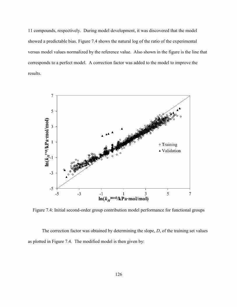
126

11 compounds, respectively. During model development, it was discovered that the model

showed a predictable bias. Figure 7.4 shows the natural log of the ratio of the experimental

versus model values normalized by the reference value. Also shown in the figure is the line that

corresponds to a perfect model. A correction factor was added to the model to improve the

results.

Figure 7.4: Initial second-order group contribution model performance for functional groups

The correction factor was obtained by determining the slope, D, of the training set values

as plotted in Figure 7.4. The modified model is then given by:

127

+

−

=

∑∑

refiii

refiii

refH

H

TTnC

TTnBD

kk ln11ln

,. 7.7

The correction factor is only necessary for alcohols, esters, ethers, and ketones. For

hydrocarbons, D equals unity. Figure 7.5 shows the corrected natural log of the ratio of the

experimental versus model values normalized by the reference value. The outliers in Figure 7.4

and Figure 7.5 are data points for 2-butoxyethanol which is a multifunctional compound.

Plyasunov et al. [247] found it necessary to provide a correction for diethers ([O-(CH2)2-O]. 2-

Butoxyethanol has a similar structure except that one ether group is replaced by a hydroxyl

group. A correction factor was not added in this study due to the limited amount of data.

However, the data from this compound suggest that correction factors may be necessary for

multifunctional compounds.

The training set was divided into 10 subgroups for 10-fold cross-validation. With three

of the folds, the learning sets were not full rank so parameters could not be determined. The

results of the remaining seven iterations were averaged for the cross-validation statistics. Overall

parameters were determined using the full training set. The model was then applied to the

validation set. Results of the 10-fold cross-validation and overall method performance are

summarized in Table 7.11. Results are shown in Figure 7.6.

128

Figure 7.5: Corrected second-order group contribution model performance for functional groups

Table 7.11: Summary of performance for second-order temperature-dependent group contribution method for esters, ethers, ketones, and alcohols

Set #Compounds AAD R2 10-Fold Cross-Validationa Avg. AAD Avg. R2

Training 83 17% 0.987 Learning 18% 0.986

Prediction 21% 0.982 Validation 11 19% 0.970 - - -

aOnly includes results of the seven iterations that were full rank

The second-order group contribution method works slightly better for hydrocarbons than

compounds with functional groups. This is not surprising due to the increased complexity of the

compound structures. In addition, there are typically less temperature-dependent data available

for the compounds with functional groups, and the data generally had higher experimental

uncertainties.

129

Figure 7.6: Plot of experimental versus model values for the second-order temperature-dependent group contribution method for esters, ethers, ketones, and alcohols

All of the temperature-dependent groups developed in the two regressions (hydrocarbon

and functional groups) and the coefficient standard errors (SE) and two-tailed p-values are

summarized in Table 7.12. Only the first four hydrocarbon groups were used in the functional

group regression. The table also includes the number of times a group appeared in a compound

(nC) and the number of times a group appeared in all of the temperature-dependent data (nG) in

the training and validation sets for each regression. The minimum and maximum temperatures

of the data corresponding to each group found in the training and validation sets is also included.

The groups with the smallest amount of data typically have the largest standard errors and p-

values. The second-order correction factor is summarized in Table 7.13. Sample calculations

are included in Appendix D.

130

Table 7.12: Summary of second-order temperature-dependent model values

Group Bi Ci Training Validation Temp. Range

Value/K SE p-value Value SE p-value nC nG nC nG K Hydrocarbon Regression

C-(C)4 -5451 2205 0.01 13.2 7.1 0.06 4 23 0 0 273-424 C-(H)(C)3 -4267 1166 0.0003 11.8 3.8 0.002 5 45 1 11 273-423 C-(H)2(C)2 868 292 0.003 -1.89 0.90 0.04 13 830 3 56 273-456 C-(H)3(C) 6820 542 < 0.0001 -18.6 1.7 < 0.0001 19 645 3 90 273-456

C-(H)2(C)(Cb) 19962 33762 0.55 -65 111 0.56 4 115 1 11 273-373 C-(H)3(Cb) 16423 33753 0.63 -52 111 0.64 7 303 1 38 262-568 Cb-(C)(Cb)2 -13358 33753 0.69 45 111 0.69 12 423 2 49 262-568 Cb-(H)(Cb)2 1870 20 < 0.0001 -4.28 0.06 < 0.0001 13 2229 2 131 262-568

Y0 0 - - 0 - - - - - - - Functional Group Regression

[CH3-CH2-O-CH2] corra

1106 5853 0.85 -6 19 0.76 2 35 0 0 269-364

[O-(CH2)2-O] corra

-26034 17351 0.14 72 56 0.20 1 11 0 0 273-373

C-(C)(H)2(O) 22467 1574 < 0.0001 -49.8 4.9 < 0.0001 39 608 7 103 269-375 C-(C)2(H)(O)

alcohol 19591 994 < 0.0001 -39.3 3.1 < 0.0001 11 174 2 20 273-373

C-(C)2(H)(O) ester

18533 6657 0.006 -38 21 0.07 2 11 0 0 273-364

C-(C)2(H)(O) ether

12226 5167 0.02 -15 17 0.37 1 40 0 0 273-334

C-(C)3(O) alcohol

18816 2525 < 0.0001 -36.8 7.9 < 0.0001 3 42 0 0 273-371

C-(C)3(O) ester 34714 6219 < 0.0001 -90 20 < 0.0001 2 21 0 0 273-354 C-(C)3(O) ether 12359 9442 0.19 -15 30 0.62 3 72 1 9 273-363

C-(CO)(C)3 -7084 15452 0.65 25 49 0.61 1 10 0 0 273-364 C-(CO)(H)(C)2 -14006 4324 0.001 46 14 0.0007 3 28 0 0 273-364 C-(CO)(H)2(C) -9550 2434 < 0.0001 32.2 7.6 < 0.0001 12 128 4 42 273-364

CO-(C)2 17819 805 < 0.0001 -37.8 2.5 < 0.0001 19 306 1 13 265-453 COO-(C)2 -5096 2902 0.08 13 9 0.17 21 259 4 42 273-365 HCOO-(C) 1855 5873 0.75 -14 19 0.47 6 50 1 14 272-364 O-(C)(H) 0 - - 0 - - 27 425 4 54 273-375

O-(C)2 -29379 5765 < 0.0001 68.9 18.7 0.0002 9 173 2 14 269-373 C-(H)3(O) 28004 7327 0.0001 -69.9 23.3 0.003 6 112 1 6 273-373

aether corrections; used in addition to group contributions

131

Table 7.13: Second-order method correction factor

Chemical Families D Value SE

Hydrocarbons 1 - Alcohols, Ketones, Esters, Ethers 0.7758 0.0034

7.3.5 Method Application Summary

The general procedure required to use the first- and second-order bond contribution

methods of this study are described in the following steps.

1. Calculate kH,ref using Equation 7.2 and the ∞∆ hydG contributions listed in

2. Table 7.7 for the first-order method and Table 7.8 for the second-order method.

3. Calculate coefficients B and C using the group contribution values listed in

4. Table 7.7 for the first-order method and Table 7.12 for the second-order method.

5. Determine coefficient D using Table 7.13 if using the second-order method.

6. Determine the final equation by combining the coefficients and reference value

using Equation 7.1 for the first-order method and Equation 7.7 for the second-

order method.

7.3.6 Method Comparison and Recommendations

The methods of this study were compared with the literature methods using data from

144 compounds used in the first- and second-order method development. The reference point

used in the Lau et al. [39] and Kühne et al. [285] methods is the recommended Smoothed or

Experimental value at 298.15 K from this study. The results are summarized in Table 7.14.

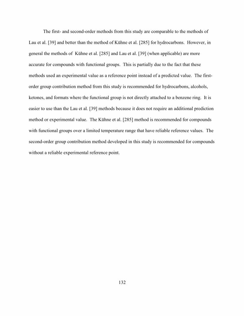
132

The first- and second-order methods from this study are comparable to the methods of

Lau et al. [39] and better than the method of Kühne et al. [285] for hydrocarbons. However, in

general the methods of Kühne et al. [285] and Lau et al. [39] (when applicable) are more

accurate for compounds with functional groups. This is partially due to the fact that these

methods used an experimental value as a reference point instead of a predicted value. The first-

order group contribution method from this study is recommended for hydrocarbons, alcohols,

ketones, and formats where the functional group is not directly attached to a benzene ring. It is

easier to use than the Lau et al. [39] methods because it does not require an additional prediction

method or experimental value. The Kühne et al. [285] method is recommended for compounds

with functional groups over a limited temperature range that have reliable reference values. The

second-order group contribution method developed in this study is recommended for compounds

without a reliable experimental reference point.

133

Table 7.14: Comparison of methods from this study with existing methods

Method Kühne AAD%

nC Lau GCM

AAD%

nC Lau BCM

AAD%

nC This study

1st order AAD%

nC This study 2nd

order AAD%

nC

Overall 49.9 144 18.6 101 11.6 50 24.2 108 24.5 125 1-Alkenes 12.2 2 21.0 2 - - 7.4 2 - - Acetates 14.9 10 - - - - - - 26.3 10

Aliphatic ethers 16.9 9 - - - - - - 25.7 9 Alkylcyclohexanes 258.4 4 11.1 4 - - 48.0 4 - -

Cycloaliphatic alcohols 9.5 1 7.0 1 - - 37.7 1 - -

Cycloalkanes 21.8 4 14.6 4 - - 52.7 4 - - Cycloalkenes 8.1 3 14.7 3 - - 40.6 3 - -

Dialkenes 10.8 1 7.4 1 - - 65.6 1 - - Dimethylalkanes 159.3 4 9.8 4 11.2 4 23.9 4 22.8 4

Formates 14.9 7 - - - - 20.9 7 33.0 7 Ketones 35.8 22 38.1 22 11.7 20 30.2 22 28.3 21

Methylalkanes 67.4 2 13.8 2 13.3 2 14.1 2 14.8 2 Methylalkenes 6.3 2 45.1 2 - - 7.5 2 - -

n-Alcohols 29.7 10 14.5 10 - - 21.5 10 17.6 10 n-Alkanes 172.9 8 14.1 8 14.5 8 16.1 8 15.6 8

n-Alkylbenzenes 21.2 7 8.9 7 8.7 7 10.1 7 8.8 7 Other aliphatic

alcohols 20.5 21 11.5 21 - - 22.1 21 22.7 21 Other alkanes 28.7 1 21.6 1 4.4 1 20.3 1 16.7 1

Other alkylbenzenes 163.2 8 10.9 8 11.4 8 14.6 8 29.8 8 Other ethers/diethers 13.1 1 - - - - -

35.1 1

Other monoaromatics 6.2 1 6.9 1 - - 6.0 1 - - Other polyfunctional

C, H, O 10.3 1 - - - - - - 89.7 1 Other saturated aliphatic esters 27.6 2 - - - - - - 37.9 2 Propionates and

butyrates 26.4 13 - - - - - - 25.5 13 < 3% 15.4 8 13.4 6 5.5 4 5.6 6 11.6 7 < 5% 41.4 25 7.5 21 7.1 9 16.6 22 17.7 21

< 10% 43.5 71 12.1 53 9.8 29 19.3 56 19.5 66 < 25% 52.1 76 31.3 51 20.1 25 36.4 54 30.7 66 < 50% 58.0 29 43.5 23 45.9 13 46.9 23 46.7 27

< 100% 68.3 15 71.1 11 75.4 8 88.0 11 71.4 13

134

135

8 Summary

A database containing recommended values for Henry’s law constants, infinite dilution

activity coefficients and solubility data of industrially important chemicals has been compiled for

aqueous systems. These properties are important in predicting the fate and transport of

chemicals in the environment. The structure of this database is compatible with the existing

DIPPR® 801 database and DIADEM interface. Recommendations have been provided for 498

compounds for at least one of the properties.

Thermodynamic relationships, chemical family trends, and predicted values were

important data analysis tools. Data from the various properties were related to each other using

thermodynamic relationships and reliable DIPPR® 801 pure component property values. For

hydrophobic compounds, the data from the three properties were combined to obtain

recommendations. In instances where the data could not be combined, the thermodynamic

relationships were helpful in identifying the best datasets. Chemical family plots were used with

temperature-dependent and single-temperature data to check for consistency within chemical

families and to select the best data. Predicted values were used to select the best datasets when

there were discrepancies in the literature data. Notes in the database provide information about

the procedure and data used to provide recommendations for each compound and property.

136

Henry’s law constants were measured for seven compounds at various temperatures and

atmospheric pressure using the inert gas stripping method. Two of these compounds were used

to validate the experimental method, and good agreement was obtained between results from this

study and literature values. The remaining compounds were chosen to clarify discrepancies

between literature values or to provide values for compounds that have not been measured.

Infinite dilution activity coefficients were determined for each compound. A fugacity ratio was

required to determine infinite dilution activity coefficients for the solid solutes. It was obtained

from the heats of fusion and the liquid and solid heat capacities for the pure solutes as obtained

from the DIPPR® 801 database. The experimental work was published [294].

A first-order temperature-dependent group contribution method was developed using the

method of Plyasunov et al. [243] as a reference point. The method works for hydrocarbons,

alcohols, ketones, and formats where none of the functional groups are directly attached to a

benzene ring. Attempts to add group contributions for ethers and esters were unsuccessful. A

second-order temperature-dependent group contribution method was developed using the groups

defined by Plyasunov et al. [244-247]. Additional second-order hydrocarbon groups were first

defined at the reference condition of 298.15 K and 100 kPa before developing temperature-

dependent parameters. The method is applicable for hydrocarbons, esters, ethers, ketones, and

alcohols. The first-order group contribution method from this study is recommended when

applicable. It is easier to use than the Lau et al. [39] methods because it does not require an

additional prediction method or experimental value. The Kühne et al. method [285] is

recommended for esters and ethers below 353 K when a reliable experimental reference value is

available. The second-order group contribution method developed in this study is recommended

for esters and ethers when a reliable experimental value is not available for a reference point.

137

8.1 Recommendations for Future Work

The 801E database could be expanded to include additional properties. As mentioned in

Section 2.1.3, derivative properties ( ∞∆ hydH , ∞∆ hydCp , and ∞V ) are thermodynamically related to

kH. These properties could be added to the database to further aid in the designation of

recommended values and the development of prediction methods.

The current database does not take into account the effects of pressure which are

significant for gases. Because of this, API recommendations were accepted (see Section 4.5).

The database could be modified to include pressure as a dependent variable. This would allow

data at intermediate and high pressures to be included. The unit conversions could be modified

in order to take into account non-idealities due to high temperatures and pressures. More data at

high temperatures and pressures could also be included for compounds that are liquids and

solids.

Although SOLC data were included in the database, no efforts were made to provide

recommended values for this property. In the future, SOLC and xiaq data could be analyzed

simultaneously to obtain the entire solubility curves for compounds with critical solution

temperatures.

Further temperature-dependent kH experiments could be performed to continue measuring

compounds with discrepancies in the literature and/or missing literature data. If temperature-

dependent regressions have been assigned high uncertainties, then the available data have

significant noise. Additional measurements could provide a better regression. In addition,

measurements could be performed for compounds with interesting chemical family trends (i.e.

cycloalkanes, cycloalkenes, n-alkanes) to provide further insights into the trends. More data

would also be useful for compounds with multiple functional groups.

138

Additional second-order group contribution reference values can be added to the

prediction method developed in this study to broaden the chemical applicability. Prediction

methods have the largest errors for compounds with multiple functional groups. Unfortunately,

limited data are available for multifunctional compounds. As mentioned, additional

experimental work could provide more data for multifunctional compounds allowing for the

development of better prediction methods.

139

9 References

1. U.S. Environmental Protection Agency, Chemistry Assistance Manual for Premanufacture Notification Submitters, 1997, Office of Pollution Prevention and Toxics, U.S. Environmental Protection Agency Washington, DC.

2. REACH. Feb. 19, 2009. European Commission. Retrieved 2009 April 8. <http://ec.europa.eu/environment/chemicals/reach/reach_intro.htm>.

3. The cost of doing business just got higher. AIChE. Retrieved 2009 April 8. <http://www.aiche.org/DIPPR/products/REACH.aspx>.

4. Physico-chemical data requirements. Department of Chemistry of the French National Centre for Scientific Research. Retrieved 2009 April 7. <http://www.prc.cnrs-gif.fr/reach/en/physicochemical_data.html>.

5. SPARC Performs Automated Reasoning in Chemistry. 10 Jan. 2013. United States Environmental Protection Agency. 24 Jan. 2013. <http://www.epa.gov/athens/research/sparc.html>.

6. Kline, A.A., et al., An overview of compiling, critically evaluating, and delivering reliable physical property data from AIChE DIPPR® Projects 911 and 912. Fluid Phase Equilib., 1998. 150-151: p. 421-428.

7. Hemond, H.F. and E.J. Fechner-Levy, Chemical fate and transport in the environment. 2000, San Diego: San Diego : Academic Press.

8. Ma, J.H.Y., et al., Temperature Dependence of the Aqueous Solubility of Selected Chlorobenzenes and Chlorotoluenes. J. Chem. Eng. Data, 2001. 46(3): p. 619-622.

9. Keeley, D.F., M.A. Hoffpauir, and J.R. Meriwether, Solubility of aromatic hydrocarbons in water and sodium chloride solutions of different ionic strengths: C2-Substituted benzenes. J. Chem. Eng. Data, 1991. 36(4): p. 456-459.

10. Pinal, R., et al., Cosolvency of partially miscible organic solvents on the solubility of hydrophobic organic chemicals. Environ. Sci. Technol., 1990. 24(5): p. 639-647.

140

11. Sawamura, S., K. Kitamura, and Y. Taniguchi, Effect of pressure on the solubilities of benzene and alkylbenzenes in water. J. Phys. Chem., 1989. 93(12): p. 4931-4935.

12. Nielsen, F., E. Olsen, and A. Fredenslund, Henry's Law Constants and Infinite Dilution Activity Coefficients for Volatile Organic Compounds in Water by a Validated Batch Air Stripping Method. Environ. Sci. Technol., 1994. 28(12): p. 2133-2138.

13. Yaws, C., H.-C. Yang, and X. Pan, Henry's Law Constants for 362 Organic Compounds in Water. Chem. Eng., 1991. 98(11): p. 179-85.

14. Dearden, J.C. and G. Schüürmann, Quantitative structure-property relationships for predicting Henry's law constant from molecular structure. Environ. Toxicol. Chem., 2003. 22(8): p. 1755-1770.

15. Moore, R.C., Henry's Law Constant for Environmentally Significant Compounds. Appl. Biochem. Biotechnol., 1992. 34-5: p. 671-680.

16. Smith, F.L. and A.H. Harvey, Avoid Common Pitfalls When Using Henry's law. Chem. Eng. Prog., 2007. 103(9): p. 33-39.

17. Prausnitz, J.M., R.N. Lichtenthaler, and E. Gomes de Azevedo, Molecular Thermodynamics of Fluid-Phase Equilibria. 3rd ed. 1999, Upper Sadle River: Prentice Hall PTR.

18. Smith, J.M., H.C. Van Ness, and M.M. Abbott, Introduction to Chemical Engineering Thermodynamics. 7th ed. Chemical Engineering Series. 2005, New York: McGraw-Hill. 817.

19. Mackay, D. and W.Y. Shiu, A Critical Review of Henry's Law Constants for Chemicals of Environmental Interest. J. Phys. Chem. Ref. Data, 1981. 10(4): p. 1175-1199.

20. Ben-Naim, A., Solvation Thermodynamics. 1987, New York: Plenum Press. pp. 246.

21. Dohnal, V., D. Fenclova, and P. Vrbka, Temperature Dependences of Limiting Activity Coefficients, Henry's Law Constants, and Derivative Infinite Dilution Properties of Lower (C1-C5) 1-Alkanols in Water. Critical Compilation, Correlation, and Recommended Data. J. Phys. Chem. Ref. Data, 2006. 35(4): p. 1621-1651.

22. Majer, V., J. Sedlbauer, and G. Bergin, Henry's law constant and related coefficients for aqueous hydrocarbons, CO2 and H2S over a wide range of temperature and pressure. Fluid Phase Equilib., 2008. 272: p. 65-74.

23. Staudinger, J. and P.V. Roberts, A critical review of Henry's law constants for environmental applications. Crit. Rev. Environ. Sci. Technol., 1996. 26(3): p. 205-297.

24. Baum, E.J., Chemical Property Estimation: Theory and Application. 1998, Boca Raton: CRC Press LLC.

141

25. Schwarz, F.P. and S.P. Wasik, A fluorescence method for the measurement of the partition coefficients of naphthalene, 1-methylnaphthalene, and 1-ethylnaphthalene in water. J. Chem. Eng. Data, 1977. 22(3): p. 270-273.

26. Sarraute, S., et al., Aqueous solubility, Henry's law constants and air/water partition coefficients of n-octane and two halogenated octanes. Chemosphere, 2004. 57(10): p. 1543-1551.

27. Betterton, E.A. and M.R. Hoffmann, Henry's law constants of some environmentally important aldehydes. Environ. Sci. Technol., 1988. 22(12): p. 1415-1418.

28. Sandler, S.I., Infinite dilution activity coefficients in chemical, environmental and biochemical engineering. Fluid Phase Equilib., 1996. 116(1-2): p. 343-353.

29. Myrdal, P., et al., AQUAFAC 1: AQUEOUS FUNCTIONAL GROUP ACTIVITY COEFFICIENTS; APPLICATION TO HYDROCARBONS. Chemosphere, 1992. 24(8): p. 1047-1061.

30. Tiegs, D., et al., Activity coefficients at infinite dilution. Chemistry Data Series, ed. D. Tiegs. 1986: Frankfurt/Main : DECHEMA ; Great Neck, N.Y. : Distributed by Scholium International.

31. Clark, M.M., Transport Modeling for Environmental Engineers and Scientists. 1996, New York: John Wiley & Sons, Inc.

32. Bahadur, N.P., et al., Temperature Dependence of Octanol-Water Partition Coefficient for Selected Chlorobenzenes. J. Chem. Eng. Data, 1997. 42(4): p. 685-688.

33. Daylight Chemical Information Systems, I. Medchem Database. 2008 BioByte Corp. Retrieved 2010 July 12. http://www.daylight.com/products/medchem.html.

34. LOGKOW©: A databank of evaluated octanol-water partition coefficients (Log P). 6 Jun 2013. Sangster Research Laboratories,. Retrieved 2013 Jun 13. http://logkow.cisti.nrc.ca/logkow/index.jsp.

35. Dohnal, V., Measurement of Limiting Activity Coefficients Using Analytical Tools, in Measurement of the Thermodynamic Properties of Multiple Phases, R.D. Weir and T.W.d. Loos, Editors. 2005, Elsevier: Amsterdam. p. 359-381.

36. Tummers, B. Datahief III. 2006; 1.5. Available from: <http://datathief.org/>.

37. Mackay, D., W.Y. Shiu, and R.P. Sutherland, Determination of air-water Henry's law constants for hydrophobic pollutants. Environ. Sci. Technol., 1979. 13(3): p. 333-337.

38. Fu, J.-K. and R.G. Luthy, Aromatic compound solubility in solvent/water mixtures. J. Environ. Eng. (N. Y.), 1986. 112(2): p. 328-45.

142

39. Lau, K., T.N. Rogers, and D.A. Zei, Modeling the temperature dependence of the Henry's law constant of organic solutes in water. Fluid Phase Equilib., 2010. 290(1–2): p. 166-180.

40. Van Noort, P.C.M., Fugacity ratio estimations for high-melting rigid aromatic compounds. Chemosphere, 2004. 56(1): p. 7-12.

41. Mackay, D., W.Y. Shiu, and K.C. Ma, Henry's Law Constant, in Handbook of Property Estimation Methods for Chemicals: Environmental and Health Sciences. 2000, Lewis Publishers. p. 69-87.

42. Prausnitz, J.M. and F.H. Shair, A Thermodynamic Correlation of Gas Solubilities. AIChE J., 1961. 7(4): p. 682-7.

43. Ginnings, P.M. and R. Baum, Aqueous Solubilities of the Isomeric Pentanols. J. Am. Chem. Soc., 1937. 59(6): p. 1111-1113.

44. Stephenson, R., J. Stuart, and M. Tabak, Mutual Solubility of Water and Aliphatic Alcohols. J. Chem. Eng. Data, 1984. 29(3): p. 287-290.

45. Kühne, R., et al., Hydrophobicity and hydrophobic interactions. II. Differentiation of surface area effects on several thermodynamic transfer data of hydrophobic solutes. Eur. J. Med. Chem. - Chim. Ther., 1981. 16(1): p. 7-12.

46. Fenclová, D., et al., Temperature Dependence of Limiting Activity Coefficients, Henry’s Law Constants, and Related Infinite Dilution Properties of Branched Pentanols in Water. Measurement, Critical Compilation, Correlation, and Recommended Data. J. Chem. Eng. Data, 2010. 55(9): p. 3032-3043.

47. Abraham, M.H., et al., Thermodynamics of solute transfer from water to hexadecane. J. Chem. Soc., Perkin Trans. 2, 1990(2): p. 291-300.

48. Dohnal, V. and D. Ondo, Refined non-steady-state gas-liquid chromatography for accurate determination of limiting activity coefficients of volatile organic compounds in water - Application to C1-C5 alkanols. J. Chromatogr., A, 2005. 1097(1-2): p. 157-164.

49. Sherman, S.R., et al., Compilation and Correlation of Limiting Activity Coefficients of Nonelectrolytes in Water. Ind. Eng. Chem. Res., 1996. 35(4): p. 1044-58.

50. Noubigh, A., et al., Solubility of Gallic Acid, Vanillin, Syringic Acid, and Protocatechuic Acid in Aqueous Sulfate Solutions from (293.15 to 318.15) K. J. Chem. Eng. Data, 2008. 53(7): p. 1675-1678.

51. Dehn, W.M., COMPARATIVE SOLUBILITIES IN WATER, IN PYRIDINE AND IN AQUEOUS PYRIDINE. J. Am. Chem. Soc., 1917. 39(7): p. 1399-1404.

52. Mange, C.E. and O. Ehler, Solubilities of Vanillin. Ind. Eng. Chem., 1924. 16(12): p. 1258-1260.

143

53. Cartwright, L.C., Vanilla-Like Synthetics: Solubility and Volatility of Propenyl Guaethol, Bourbonal, Vanillin, and Coumarin. J. Agric. Food. Chem., 1953. 1(4): p. 312-314.

54. Noubigh, A., M. Abderrabba, and E. Provost, Temperature and salt addition effects on the solubility behaviour of some phenolic compounds in water. J. Chem. Thermodynamics, 2007. 39(2): p. 297-303.

55. Bozdag, O. and J.A. Lamb, Dependence of the mutual solubilities of (2-butanol+water) upon pressure and temperature. J. Chem. Thermodynamics, 1983. 15(2): p. 165-171.

56. Hafter, G.T., A.F.M. Barton, and A. Chand, Semi-automated apparatus for the determination of liquid solubilities: mutual solubilities of water and butan-2-ol. J. Chem. Soc., Faraday Trans., 1991. 87(4): p. 591-596.

57. Ochi, K., T. Saito, and K. Kojima, Measurement and Correlation of Mutual Solubilities in 2-Butanol + Water. J. Chem. Eng. Data, 1996. 41(2): p. 361-364.

58. Moriyoshi, T., et al., Mutual solubility of 2-butanol + water under high pressure. J. Chem. Thermodynamics, 1975. 7(6): p. 537-545.

59. Evans, T.W., The Hill Method for Solubility Determinations. Ind. Eng. Chem. Anal. Ed., 1936. 8(3): p. 206-208.

60. Letcher, T.M. and P.M. Siswana, Liquid-liquid equilibria for mixtures of an alkanol + water + a methyl substituted benzene at 25°C. Fluid Phase Equilib., 1992. 74(0): p. 203-217.

61. Letcher, T.M., S. Ravindran, and S. Radloff, Liquid-liquid equilibria for mixtures of an alkanol + diisopropyl ether + water at 25°C. Fluid Phase Equilib., 1992. 71(1–2): p. 177-188.

62. De Santis, R., L. Marrelli, and P.N. Muscetta, Liquid—liquid equilibria in water—aliphatic alcohol systems in the presence of sodium chloride. Chem. Eng. J., 1976. 11(3): p. 207-214.

63. Jaoui, M., M. Luszczyk, and M. Rogalski, Liquid−Liquid and Liquid−Solid Equilibria of Systems Containing Water and Selected Chlorophenols. J. Chem. Eng. Data, 1999. 44(6): p. 1269-1272.

64. Sidgwick, N.V. and S.L. Turner, The Solubility of the Chlorophenols. J. Chem. Soc., 1922. 121: p. 2256-2263.

65. Achard, C., et al., Aqueous Solubilities of Phenol Derivatives by Conductivity Measurements. J. Chem. Eng. Data, 1996. 41(3): p. 504-507.

66. Blackman, G.E., M.H. Parke, and G. Garton, The physiological activity of substituted phenols. II. Relationships between physical properties and physiological activity. Arch. Biochem. Biophys., 1955. 54(1): p. 55-71.

144

67. Ma, K.C., W.Y. Shiu, and D. Mackay, Aqueous Solubilities of Chlorinated Phenols at 25°C. J. Chem. Eng. Data, 1993. 38(3): p. 364-366.

68. Lei, Y.D., C. Shunthirasingham, and F. Wania, Comparison of Headspace and Gas-Stripping Techniques for Measuring the Air-Water Partititioning of Normal Alkanols (C4 to C10): Effect of Temperature, Chain Length, and Adsorption to the Water Surface. J. Chem. Eng. Data, 2007. 52(1): p. 168-179.

69. Tochigi, K., M. Uchiyama, and K. Kojima, Measurement of infinite-dilution activity coefficients of alcohols in water using relative gas-liquid chromatographic method. Korean J. Chem. Eng., 2000. 17(5): p. 502-505.

70. Altschuh, J., et al., Henry's law constants for a diverse set of organic chemicals: experimental determination and comparison of estimation methods. Chemosphere, 1999. 39(11): p. 1871-1887.

71. Shiu, W.-Y. and D. Mackay, Henry's Law Constants of Selected Aromatic Hydrocarbons, Alcohols, and Ketones. J. Chem. Eng. Data, 1997. 42(1): p. 27-30.

72. Tewari, Y.B., et al., Aqueous solubility and octanol/water partition coefficient of organic compounds at 25.0°C. J. Chem. Eng. Data, 1982. 27(4): p. 451-454.

73. Addison, C.C., 26. The properties of freshly formed surfaces. Part IV. The influence of chain length and structure on the static and the dynamic surface tensions of aqueousalcoholic solutions. J. Chem. Soc., 1945: p. 98-106.

74. Li, A. and A.W. Andren, Solubility of polychlorinated biphenyls in water/alcohol mixtures. 1. Experimental data. Environ. Sci. Technol., 1994. 28(1): p. 47-52.

75. Kinoshita, K., H. Ishikawa, and K. Shinoda, Solubility of Alcohols in Water Determined by the Surface Tension Measurements. Bull. Chem. Soc. Jpn., 1958. 31(9): p. 1081-1082.

76. Hill, D.J.T. and L.R. White, The Enthalpies of Solution of Hexan-1-ol and Heptan-1-ol in Water. Aust. J. Chem., 1974. 27: p. 1905-1916.

77. Butler, J.A.V., D.W. Thomson, and W.H. Maclennan, 173. The free energy of the normal aliphatic alcohols in aqueous solution. Part I. The partial vapour pressures of aqueous solutions of methyl, n-propyl, and n-butyl alcohols. Part II. The solubilities of some normal aliphatic alcohols in water. Part III. The theory of binary solutions, and its application to aqueous-alcoholic solutions. J. Chem. Soc., 1933: p. 674-686.

78. Vochten, R. and G. Petre, Study of the heat of reversible adsorption at the air-solution interface. II. Experimental determination of the heat of reversible adsorption of some alcohols. J. Colloid Interface Sci., 1973. 42(2): p. 320-327.

79. Shchelokova, E.A., et al., Solubility of monohydric aliphatic alcohols in water and aqueous HCl solutions. Russ. J. Appl. Chem., 2012. 85(3): p. 465-469.

145

80. Rao, K.S., M.V.R. Rao, and C.V. Rao, Ternary Liquid Equilibria: Acetone-water-n-heptanol & Acetone-water-n-octanol Systems. J. Sci. Industr. Res., 1961. 20B: p. 283-6.

81. Tsonopoulos, C., Thermodynamic analysis of the mutual solubilities of normal alkanes and water. Fluid Phase Equilib., 1999. 156(1–2): p. 21-33.

82. Tsonopoulos, C., Thermodynamic analysis of the mutual solubilities of hydrocarbons and water. Fluid Phase Equilib., 2001. 186(1–2): p. 185-206.

83. HENRYWIN--Version3.20. 2011.

84. Ryu, S.-A. and S.-J. Park, Determination of the air/water partition coefficient for environmental pollutants by using the modified EPICS method and the relationship between the partition coefficient and physical properties. Hwahak Konghak, 1998. 36(4): p. 554-561.

85. Coates, M., D.W. Connell, and D.M. Barron, Aqueous solubility and octan-1-ol-water partition coefficients of aliphatic hydrocarbons. Environ. Sci. Technol., 1985. 19(7): p. 628-632.

86. McAuliffe, C., Solubility in Water of Paraffin, Cycloparaffin, Olefin, Acetylene, Cycloolefin, and Aromatic Hydrocarbons. J. Phys. Chem., 1966. 70(4): p. 1267-1275.

87. Leinonen, P.J. and D. Mackay, The multicomponent solubility of hydrocarbons in water. Can. J. Chem. Eng., 1973. 51(2): p. 230-233.

88. Letinski, D.J., et al., Slow-stir water solubility measurements of selected alcohols and diesters. Chemosphere, 2002. 48(3): p. 257-265.

89. Hoffman, C.S. and E.W. Anacker, Water solubilities of tetradecanol and hexadecanol. J. Chromatogr., 1967. 30(2): p. 390-6.

90. Robb, I.D., Determination of the aqueous solubility of fatty acids and alcohols. Aust. J. Chem., 1966. 19(12): p. 2281-2284.

91. Stephenson, R. and J. Stuart, Mutual binary solubilities: water-alcohols and water-esters. J. Chem. Eng. Data, 1986. 31(1): p. 56-70.

92. Krause, F.P. and W. Lange, Aqueous solubilities of n-dodecanol, n-hexadecanol, and n-octadecanol by a new method. J. Phys. Chem., 1965. 69(9): p. 3171-3.

93. Kırbaşlar, Ş.İ., S. Şahin, and M. Bilgin, (Liquid + liquid) equilibria of (water + propionic acid + alcohol) ternary systems. J. Chem. Thermodynamics, 2006. 38(12): p. 1503-1509.

94. Ferguson, A.L., P.G. Debenedetti, and A.Z. Panagiotopoulos, Solubility and Molecular Conformations of n-Alkane Chains in Water. J. Phys. Chem. B, 2009. 113(18): p. 6405-6414.

146

95. Tolls, J., et al., Aqueous Solubility−Molecular Size Relationships:  A Mechanistic Case Study Using C10- to C19-Alkanes. The Journal of Physical Chemistry A, 2002. 106(11): p. 2760-2765.

96. Mackay, D., W.Y. Shiu, and A.W. Wolkoff, Gas Chromatographic Determination of Low Concentrations of Hydrocarbons in Water by Vapor Phase Extraction. ASTM Spec. Tech. Publ., 1975. 573(Water Quality Parameters Symposium): p. 251-8.

97. McAuliffe, C., Solubility in water of normal C9 and C10 alkane hydrocarbons. Science (New York, N.Y.), 1969. 163(3866): p. 478-9.

98. Sutton, C. and J.A. Calder, Solubility of higher-molecular-weight normal-paraffins in distilled water and sea water. Environ. Sci. Technol., 1974. 8(7): p. 654-657.

99. Franks, F., Solute-water interactions and the solubility behavior of long-chain paraffin hydrocarbons. Nature (London, U. K.), 1966. 210(5031): p. 87-8.

100. McBain, J.W. and P.H. Richards, Solubilization of Insoluble Organic Liquids by Detergents. Ind. Eng. Chem., 1946. 38(6): p. 642-646.

101. Peake, E. and G.W. Hodgson, Alkanes in aqueous systems. I. Exploratory investigations on the accommodation of C20-C33 n-alkanes in distilled water and occurrence in natural water systems. J. Am. Oil Chem. Soc., 1966. 43(4): p. 215-22.

102. Baker, E.G., Origin and migration of oil. Science (Washington, DC, U. S.), 1959. 129: p. 871-4.

103. Hellinger, S. and S.I. Sandler, Liquid-Liquid Equilibria of Fuel Oxygenate + Water + Hydrocarbon Mixtures. 2. J. Chem. Eng. Data, 1995. 40(1): p. 321-325.

104. Krasnoshchekova, R.Y. and M. Gubergrits, Solubility of paraffin hydrocarbons in fresh and salt water. Neftekhimiya, 1973. 13(6): p. 885-8.

105. Ben-Naim, A. and J. Wilf, Solubilities and hydrophobic interactions in aqueous solutions of monoalkylbenzene molecules. J. Phys. Chem., 1980. 84(6): p. 583-586.

106. Sherblom, P.M., P.M. Gschwend, and R.P. Eganhouse, Aqueous solubilities, vapor pressures, and 1-octanol-water partition coefficients for C9-C14 linear alkylbenzenes. J. Chem. Eng. Data, 1992. 37(4): p. 394-9.

107. Řehák, K., et al., (Liquid + liquid) equilibrium for (dimethyl phthalate + water), (diethyl phthalate + water), and (dibutyl phthalate + water). J. Chem. Thermodynamics, 2000. 32(3): p. 393-400.

108. Kırbaşlar, Ş.İ., S. Şahin, and M. Bilgin, (Liquid+liquid) equilibria of (water + butyric acid + esters) ternary systems. J. Chem. Thermodynamics, 2007. 39(9): p. 1279-1285.

147

109. Wolfe, N.L., W.C. Steen, and L.A. Burns, Phthalate ester hydrolysis: Linear free energy relationships. Chemosphere, 1980. 9(7–8): p. 403-408.

110. Howard, P.H., S. Banerjee, and K.H. Robillard, Measurement of water solubilities, octanol/water partition coefficients and vapor pressures of commercial phthalate esters. Environ. Toxicol. Chem., 1985. 4(5): p. 653-661.

111. Thomsen, M., L. Carlsen, and S. Hvidt, Solubilities and surface activities of phthalates investigated by surface tension measurements. Environ. Toxicol. Chem., 2001. 20(1): p. 127-132.

112. Leyder, F. and P. Boulanger, Ultraviolet absorption, aqueous solubility, and octanol-water partition for several phthalates. Bull. Environ. Contam. Toxicol., 1983. 30(2): p. 152-7.

113. Russell, D.J., Transport and Fate of Organic Pollutants in the Environment with Emphasis on Phthalate Esters, Ph.D., State University of New York at Binghamton, New York. 1983.

114. Defoe, D.L., et al., Solubility and toxicity of eight phthalate esters to four aquatic organisms. Environ. Toxicol. Chem., 1990. 9(5): p. 623-636.

115. Ellington, J.J., Octanol/Water Partition Coefficients and Water Solubilities of Phthalate Esters†. J. Chem. Eng. Data, 1999. 44(6): p. 1414-1418.

116. Fishbein, L. and P.W. Albro, Chromatographic and biological aspects of the phthalate esters. J. Chromatogr., 1972. 70(2): p. 365-412.

117. Rowley, R.L., et al., DIPPR® Data Compilation of Pure Chemical Properties, Design Institue for Physical Properties, AIChE, New York, NY (2011).

118. Vesala, A., Thermodynamics of transfer of nonelectrolytes from light to heavy water. I. Linear free energy correlations of free energy of transfer with solubility and heat of melting of a nonelectrolyte. Acta Chem. Scand., Ser. A, 1974. A28(8): p. 839-45.

119. Stephenson, R.M., Mutual solubility of water and aliphatic amines. J. Chem. Eng. Data, 1993. 38(4): p. 625-629.

120. Hales, B.J., G.L. Bertrand, and L.G. Hepler, Effects of Third Components on Critical Mixing in the Water-Triethylamine System. J. Phys. Chem., 1966. 70(12): p. 3970-3975.

121. De Santis, R., Phase equilibriums of the water-sodium chloride-triethylamine system. J. Chem. Eng. Data, 1976. 21(3): p. 328-330.

122. Kitamura, N., et al., Laser-induced liquid-to-droplet extraction of chlorophenol: photothermal phase separation of aqueous triethylamine solutions. Anal. Chem., 2005. 77(18): p. 6055-61.

148

123. Mendonça, Â.F.S.S., S.N.R. Pereira, and I.M.S. Lampreia, Solubility of Triethylamine in Calcium Chloride Aqueous Solutions from 20 to 35°C. J. Solution Chem., 2003. 32(12): p. 1033-1044.

124. Ishiguro, T., et al., Equilibria of the systems amine-water-caustic alkali. II. Mutual solubilities of Et3N-H2O-NaOH and Et3N-H2O-KOH systems. Yakugaku Zasshi, 1955. 75: p. 188-92.

125. Wenzel, J., et al., Kinetics of phase separation in binary liquid mixtures. J. Phys. Chem., 1980. 84(15): p. 1991-1995.

126. Davidson, R.R., W.H. Smith, and D.W. Hood, Structure and Amine-Water Solubility in Desalination by Solvent Extraction. J. Chem. Eng. Data, 1960. 5(4): p. 420-423.

127. Kohler, F. and O.K. Rice, Coexistence Curve of the Triethylamine-Water System. J. Chem. Phys., 1957. 26(6): p. 1614-1618.

128. API Technical Data Book--Version 9.0, 2006, The American Petroleum Institute and EPCON International.

129. Horvath, A.L. and F.W. Getzen, IUPAC-NIST Solubility Data Series 68. Halogenated Aliphatic Hydrocarbon Compounds C3-C14 With Water. J. Phys. Chem. Ref. Data, 1999. 28(3): p. 649-777.

130. Horvath, A.L., F.W. Getzen, and Z. Maczynska, IUPAC-NIST Solubility Data Series 67. Halogenated Ethanes and Ethenes with Water. J. Phys. Chem. Ref. Data, 1999. 28(2): p. 395-627.

131. Sazonov, V.P., K.N. Marsh, and G.T. Hefter, IUPAC-NIST Solubility Data Series 71. Nitromethane with Water or Organic Solvents: Binary Systems. J. Phys. Chem. Ref. Data, 2001. 29(5): p. 1165-1354.

132. Sazonov, V.P., et al., IUPAC-NIST Solubility Data Series. 78. Acetonitrile Binary Systems. J. Phys. Chem. Ref. Data, 2002. 31(4): p. 989-1133.

133. Sazonov, V.P., K.N. Marsh, and G.T. Hefter, IUPAC-NIST solubility data series 71. Nitromethanes with water or organic solvents: binary systems. [Erratum to document cited in CA134:301421]. J. Phys. Chem. Ref. Data, 2002. 31(2): p. 699.

134. Sazonov, V.P., D.G. Shaw, and K.N. Marsh, IUPAC-NIST solubility data series. 77. C2+ nitroalkanes with water or organic solvents: binary and multicomponent systems. J. Phys. Chem. Ref. Data, 2002. 31(1): p. 1-121.

135. Clever, H.L., et al., IUPAC-NIST Solubility Data Series. 80. Gaseous fluorides of boron, nitrogen, sulfur, carbon, and silicon and solid xenon fluorides in all solvents. [Erratum to document cited in CA143:160456]. J. Phys. Chem. Ref. Data, 2005. 34(4): p. 2347-2349.

149

136. Shaw, D.G., et al., IUPAC-NIST Solubility Data Series. 81. Hydrocarbons with Water and Seawater-Revised and Updated. Part 8. C9 Hydrocarbons with Water. J. Phys. Chem. Ref. Data, 2005. 34(4): p. 2299-2345.

137. Shaw, D.G., et al., IUPAC-NIST Solubility Data Series. 81. Hydrocarbons with Water and Seawater Revised and Updated. Part 7. C8H12-C8H18 Hydrocarbons with Water. J. Phys. Chem. Ref. Data, 2005. 34(4): p. 2261-2298.

138. Shaw, D.G., et al., IUPAC-NIST Solubility Data Series. 81. Hydrocarbons with water and seawater-revised and updated. Part 6. C8H8-C8H10 Hydrocarbons with water. J. Phys. Chem. Ref. Data, 2005. 34(3): p. 1489-1553.

139. Maczynski, A., et al., IUPAC-NIST Solubility Data Series. 81. Hydrocarbons with water and seawater-revised and updated. Part 5. C7 Hydrocarbons with water and heavy water. J. Phys. Chem. Ref. Data, 2005. 34(3): p. 1399-1487.

140. Maczynski, A., et al., IUPAC-NIST Solubility Data Series. 81. Hydrocarbons with water and seawater-Revised and updated. Part 4. C6H14 Hydrocarbons with water. J. Phys. Chem. Ref. Data, 2005. 34(2): p. 709-753.

141. Maczynski, A., et al., IUPAC-NIST Solubility Data Series. 81. Hydrocarbons with water and seawater-revised and updated. Part 3. C6H8 - C6H12 hydrocarbons with water and heavy water. J. Phys. Chem. Ref. Data, 2005. 34(2): p. 657-708.

142. Maczynski, A., et al., IUPAC-NIST Solubility Data Series. 81. Hydrocarbons with water and seawater-revised and updated. Part 2. Benzene with water and heavy water. J. Phys. Chem. Ref. Data, 2005. 34(2): p. 477-552.

143. Maczynski, A., et al., IUPAC-NIST Solubility Data Series. 81. Hydrocarbons with Water and Seawater-Revised and updated Part 1. C5 Hydrocarbons with Water. J. Phys. Chem. Ref. Data, 2005. 34(2): p. 441-476.

144. Shaw, D.G., et al., IUPAC-NIST Solubility Data Series. 81. Hydrocarbons with Water and Seawater-Revised and Updated Part 12. C5-C26 Hydrocarbons with Seawater. J. Phys. Chem. Ref. Data, 2006. 35(2): p. 785-838.

145. Shaw, D.G., et al., IUPAC-NIST Solubility Data Series. 81. Hydrocarbons with Water and Seawater-Revised and Updated. Part 11. C13-C36 Hydrocarbons with Water. J. Phys. Chem. Ref. Data, 2006. 35(2): p. 687-784.

146. Shaw, D.G., et al., IUPAC-NIST Solubility Data Series. 81. Hydrocarbons with Water and Seawater-Revised and Updated. Part 10. C11 and C12 Hydrocarbons with Water. J. Phys. Chem. Ref. Data, 2006. 35(1): p. 153-203.

147. Shaw, D.G., et al., IUPAC-NIST Solubility Data Series. 81. Hydrocarbons with Water and Seawater-Revised and Updated. Part 9. C10 Hydrocarbons with Water. J. Phys. Chem. Ref. Data, 2006. 35(1): p. 93-151.

150

148. Maczynski, A., et al., IUPAC-NIST Solubility Data Series. 82. Alcohols with Water-Revised and Updated: Part 5. C8-C17 Alcohols with Water. J. Phys. Chem. Ref. Data, 2007. 36(3): p. 685-731.

149. Maczynski, A., et al., IUPAC-NIST Solubility Data Series. 82. Alcohols with water-revised and updated: part 4. C7 Alcohols with water. J. Phys. Chem. Ref. Data, 2007. 36(2): p. 445-484.

150. Maczynski, A., et al., IUPAC-NIST Solubility Data Series. 82. Alcohols with water-revised and updated: Part 3. C6 Alcohols with water. J. Phys. Chem. Ref. Data, 2007. 36(2): p. 399-443.

151. Maczynski, A., et al., IUPAC-NIST Solubility Data Series. 82. Alcohols with Water-Revised and Updated: Part 1. C4 Alcohols with Water. J. Phys. Chem. Ref. Data, 2007. 36(1): p. 59-132.

152. Maczynski, A., et al., IUPAC-NIST Solubility Data Series. 82: Alcohols with Water-Revised and Updated: Part 2. C5 Alcohols with Water. J. Phys. Chem. Ref. Data, 2007. 36(1): p. 133-190.

153. Maczynski, A., et al., IUPAC-NIST Solubility Data Series. 86. Ethers and ketones with water. Part 6. C7-C12 Ketones with water. J. Phys. Chem. Ref. Data, 2008. 37(3): p. 1611-1653.

154. Maczynski, A., et al., IUPAC-NIST Solubility Data Series. 86. Ethers and ketones with water. Part 5. C6 Ketones with water. J. Phys. Chem. Ref. Data, 2008. 37(3): p. 1575-1609.

155. Maczynski, A., et al., IUPAC-NIST Solubility Data Series. 86. Ethers and ketones with water. Part 4. C4 and C5 Ketones with water. J. Phys. Chem. Ref. Data, 2008. 37(3): p. 1517-1574.

156. Maczynski, A., et al., IUPAC-NIST Solubility Data Series. 86. Ethers and Ketones with Water. Part 3. C7-C14 Ethers with Water. J. Phys. Chem. Ref. Data, 2008. 37(2): p. 1169-1182.

157. Maczynski, A., et al., IUPAC-NIST Solubility Data Series. 86. Ethers and ketones with water. Part 2. C6 Ethers with water. J. Phys. Chem. Ref. Data, 2008. 37(2): p. 1147-1168.

158. Maczynski, A., et al., IUPAC-NIST Solubility Data Series. 86. Ethers and ketones with water. Part 1. C2-C5 Ethers with water. J. Phys. Chem. Ref. Data, 2008. 37(2): p. 1119-1146.

159. Goral, M., et al., IUPAC-NIST Solubility Data Series. 88. Esters with water-revised and updated. Part 1. C2 to C4 Esters. J. Phys. Chem. Ref. Data, 2009. 38(4): p. 1093-1127.

160. Goral, M., et al., IUPAC-NIST Solubility Data Series. 88. Esters with water-revised and updated. Part 4. C10 to C32 Esters. J. Phys. Chem. Ref. Data, 2010. 39(3): p. 033107/1-033107/38.

161. Harvey, A.H. and M. Salomon, Editorial: IUPAC-NIST Solubility Data Series. J. Phys. Chem. Ref. Data, 2010. 39(2): p. 020401/1.

151

162. Goral, M., et al., IUPAC-NIST Solubility Data Series. 88. Esters with water. Revised and updated. Part 3. C7 to C9 Esters. J. Phys. Chem. Ref. Data, 2010. 39(2): p. 023102/1-023102/70.

163. Goral, M., et al., IUPAC-NIST Solubility Data Series. 88. Esters with Water-Revised and Updated. Part 2: C5 and C6 Esters. J. Phys. Chem. Ref. Data, 2010. 39(1): p. 013102/1-013102/58.

164. Goral, M., et al., IUPAC-NIST Solubility Data Series. 91. Phenols with Water. Part 2. C8 to C15 Alkane Phenols with Water. J. Phys. Chem. Ref. Data, 2011. 40(3): p. 033103/1-033103/60.

165. Goral, M., et al., IUPAC-NIST Solubility Data Series. 91. Phenols with Water. Part 1. C6 and C7 Phenols with Water and Heavy Water. J. Phys. Chem. Ref. Data, 2011. 40(3): p. 033102/1-033102/46.

166. Goral, M., B. Wisniewska-Goclowska, and A. Maczynski, Recommended Liquid--Liquid Equilibrium Data. Part 4. 1-Alkanol--Water Systems. J. Phys. Chem. Ref. Data, 2006. 35(3): p. 1391-1414.

167. O’Farrell, C.E. and W.E. Waghorne, Henry’s Law Constants of Organic Compounds in Water and n-Octane at T = 293.2 K. J. Chem. Eng. Data, 2010. 55(4): p. 1655-1658.

168. Vrbka, P., et al., Measurement of infinite dilution activity coefficients of 1-alkanols (C1–C5) in water as a function of temperature (273–373 K). Fluid Phase Equilib., 2005. 237(1–2): p. 123-129.

169. Burnett, M.G., Determination of partition coefficients at infinite dilution by the gas chromatographic analysis of the vapor above dilute solutions. Anal. Chem., 1963. 35(11): p. 1567-70.

170. Snider, J.R. and G.A. Dawson, Tropospheric light alcohols, carbonyls, and acetonitrile: Concentrations in the southwestern United States and Henry's Law data. J. Geophys. Res. Atmos., 1985. 90(D2): p. 3797-3805.

171. Gupta, A.K., et al., Henry's constants of n-alkanols (methanol through n-hexanol) in water at temperatures between 40°C and 90°C. Fluid Phase Equilib., 2000. 170(2): p. 183-192.

172. Li, J. and P.W. Carr, Measurement of water-hexadecane partition coefficients by headspace gas chromatography and calculation of limiting activity coefficients in water. Anal. Chem., 1993. 65(10): p. 1443-50.

173. Pividal, K.A., A. Birtigh, and S.I. Sandler, Infinite dilution activity coefficients for oxygenate systems determined using a differential static cell. J. Chem. Eng. Data, 1992. 37(4): p. 484-487.

174. Dalager, P., Vapor-liquid equilibriums of binary systems of water with methanol and ethanol at extreme dilution of the alcohols. J. Chem. Eng. Data, 1969. 14(3): p. 298-301.

152

175. Landau, I., A.J. Belfer, and D.C. Locke, Measurement of limiting activity coefficients using non-steady-state gas chromatography. Ind. Eng. Chem. Res., 1991. 30(8): p. 1900-1906.

176. Lebert, A. and D. Richon, Infinite dilution activity coefficients of n-alcohols as a function of dextrin concentration in water-dextrin systems. J. Agric. Food. Chem., 1984. 32(5): p. 1156-1161.

177. Butler, J.A.V., C.N. Ramchandani, and D.W. Thomson, The solubility of nonelectrolytes. I. Free energy of hydration of some aliphatic alcohols. J. Chem. Soc., 1935: p. 280-5.

178. Kaneko, T., P.Y. Wang, and A. Sato, Partition coefficients of some acetate esters and alcohols in water, blood, olive oil, and rat tissues. Occup. Environ. Med., 1994. 51(1): p. 68-72.

179. Kojima, K., et al., Determination of vapor-liquid equilibriums from boiling point curves. Kagaku Kogaku, 1968. 32(2): p. 149-53.

180. Hofstee, T., A. Kwantes, and G.W.A. Rijnders, Determination of activity coefficients at infinite dilution by gas-liquid chromatography. Proc. Intern. Symposium Distillation, Brighton, England, 1960: p. 105-9.

181. Hardy, C.J., Determination of activity coefficients at infinite dilution from gas chromatographic measurements. J. Chromatogr., 1959. 2: p. 490-8.

182. Rytting, J.H., L.P. Huston, and T. Higuchi, Thermodynamic group contributions for hydroxyl, amino, and methylene groups. J. Pharm. Sci., 1978. 67(5): p. 615-618.

183. Rius, A. and C. Alfonso, Liquid-liquid equilibriums. Systems water-propyl formate and formic acid-propyl formate. An. R. Soc. Esp. Fis. Quim., Ser. B, 1955. 51B: p. 649-58.

184. Kendall, J. and L.E. Harrison, Part II. Intermediate addition-compounds and chain reactions. Compound formation in ester-water systems. Trans. Faraday Soc., 1928. 24(0): p. 588-596.

185. Goral, M., A. Maczynski, and P. Oracz, Recommended Liquid-Liquid Equilibrium Data. Part 5. Ether-Water Systems. J. Phys. Chem. Ref. Data, 2007. 36(4): p. 1399-1415.

186. Atik, Z., et al., Measurement of Activity Coefficients at Infinite Dilution of Benzene, Toluene, Ethanol, Esters, Ketones, and Ethers at Various Temperatures in Water Using the Dilutor Technique. J. Chem. Eng. Data, 2004. 49(5): p. 1429-1432.

187. Li, J., et al., Measurement of large infinite dilution activity coefficients of nonelectrolytes in water by inert gas stripping and gas chromatography. Anal. Chem., 1993. 65(22): p. 3212-3218.

188. Hartkopf, A. and B.L. Karger, Study of the interfacial properties of water by gas chromatography. Acc. Chem. Res., 1973. 6(6): p. 209-216.

153

189. Bennett, G.M. and W.G. Philip, Influence of Structure on the Solubilities of Ethers. Part I. Aliphatic Ethers. J. Chem. Soc., 1928: p. 1930-7.

190. Ginnings, P.M. and R. Webb, Aqueous Solubilities of Some Isomeric Hexanols. J. Am. Chem. Soc., 1938. 60(6): p. 1388-1389.

191. Sedlbauer, J., G. Bergin, and V. Majer, Group contribution method for Henry's Law constant of aqueous hydrocarbons. AIChE J., 2002. 48(12): p. 2936-2959.

192. Sanemasa, I., et al., Solubility measurements of benzene and the alkylbenzenes in water by making use of solute vapor. Bull. Chem. Soc. Jpn., 1982. 55(4): p. 1054-62.

193. Glew, D.N. and R.E. Robertson, The Spectrophotometric Determination of the Solubility of Cumene in Water by a Kinetic Method. J. Phys. Chem., 1956. 60: p. 332-337.

194. Howe, G.B., M.E. Mullins, and T.N. Rogers, Evaluation and prediction of Henry's law constants and aqueous solubilities for solvents and hydrocarbon fuel components. Volume 1. Technical discussion, 1987, Research Triangle Inst., Research Triangle Park, NC, USA. pp. 97.

195. Polak, J. and B.C.Y. Lu, Mutual Solubilities of Hydrocarbons and Water at 0 and 25 °C. Can. J. Chem., 1973. 51(24): p. 4018-23.

196. Leroi, J.C., et al., Accurate measurement of activity coefficients at infinite dilution by inert gas stripping and gas chromatography. Ind. Eng. Chem., Process Des. Dev., 1977. 16(1): p. 139-44.

197. Duhem, P. and J. Vidal, Extension of the Dilutor Method to Measurement of High Activity Coefficients at Infinite Dilution. Fluid Phase Equilib., 1978. 2: p. 231-235.

198. Krummen, M., D. Gruber, and J. Gmehling, Measurement of Activity Coefficients at Infinite Dilution in Solvent Mixtures Using the Dilutor Technique. Ind. Eng. Chem. Res., 2000. 39(6): p. 2114-2123.

199. Hovorka, Š. and V. Dohnal, Determination of Air−Water Partitioning of Volatile Halogenated Hydrocarbons by the Inert Gas Stripping Method. J. Chem. Eng. Data, 1997. 42(5): p. 924-933.

200. Dohányosová, P., et al., Measurement of Aqueous Solubility of Hydrophobic Volatile Organic Compounds by Solute Vapor Absorption Technique:  Toluene, Ethylbenzene, Propylbenzene, and Butylbenzene at Temperatures from 273 K to 328 K. J. Chem. Eng. Data, 2001. 46(6): p. 1533-1539.

201. Sanemasa, I., et al., Solubilities of benzene and the alkylbenzenes in water. Method for obtaining aqueous solutions saturated with vapors in equilibrium with organic liquids. Chem. Lett., 1981(2): p. 225-8.

154

202. Buttery, R.G., L. Ling, and D.G. Guadagni, Food volatiles. Volatilities of aldehydes, ketones, and esters in dilute water solution. J. Agr. Food Chem., 1969. 17(2): p. 385-9.

203. Butler, J.A.V. and W.S. Reid, The solubility of non-electrolytes. Part III. The entropy of hydration. J. Chem. Soc., 1936: p. 1171-1173.

204. Hovorka, Š., et al., Determination of temperature dependence of limiting activity coefficients for a group of moderately hydrophobic organic solutes in water. Fluid Phase Equilib., 2002. 201(1): p. 135-164.

205. Shiu, W.-Y., et al., Temperature Dependence of Aqueous Solubility of Selected Chlorobenzenes, Polychlorinated Biphenyls, and Dibenzofuran. J. Chem. Eng. Data, 1997. 42(2): p. 293-297.

206. Dewulf, J., H. Van Langenhove, and P. Everaert, Determination of Henry's law coefficients by combination of the equilibrium partitioning in closed systems and solid-phase microextraction techniques. J. Chromatogr. A, 1999. 830(2): p. 353-363.

207. Yalkowsky, S.H., R.J. Orr, and S.C. Valvani, Solubility and Partitioning. 3. The Solubility of Halobenzenes in Water. Ind. Eng. Chem. Fundam., 1979. 18(4): p. 351-353.

208. Dreisbach, R.R., Physical Properties Of Chemical Compounds, in Physical Properties of Chemical Compounds. 1961, American Chemical Society. p. 3-523.

209. Ten Hulscher, T.E.M., L.E. van der Velde, and W.A. Bruggeman, Temperature dependence of Henry's law constants for selected chlorobenzenes, polychlorinated biphenyls and polycyclic aromatic hydrocarbons. Environ. Toxicol. Chem., 1992. 11: p. 1595-1603.

210. Banerjee, S., Solubility of organic mixtures in water. Environ. Sci. Technol., 1984. 18(8): p. 587-591.

211. Chin, Y.P., W.J. Weber, Jr., and T.C. Voice, Determination of partition coefficients and aqueous solubilities by reverse phase chromatography - II. Evaluation of partitioning and solubility models. Water Res., 1986. 20(11): p. 1443-50.

212. Finizio, A. and A. Di Guardo, Estimating temperature dependence of solubility and octanol–water partition coefficient for organic compounds using RP-HPLC. Chemosphere, 2001. 45(6–7): p. 1063-1070.

213. Miller, M.M., et al., Aqueous Solubilities, Octanol/Water Partition Coefficients, and Entropies of Melting of Chlorinated Benzenes and Biphenyls. J. Chem. Eng. Data, 1984. 29: p. 184-190.

214. Boyd, E.M., et al., Toxicity of chlorobenzenes to a lux-marked terrestrial bacterium, Pseudomonas fluorescens. Environ. Toxicol. Chem., 1998. 17(11): p. 2134-2140.

155

215. Booth, H.S. and H.E. Everson, Hydrotropic Solubilities: Solubilities in 40 Per Cent Sodium Xylenesulfonate. J. Ind. Eng. Chem., 1948. 40(8): p. 1491-1493.

216. Stephenson, R.M., Mutual solubilities: water-ketones, water-ethers, and water-gasoline-alcohols. J. Chem. Eng. Data, 1992. 37(1): p. 80-95.

217. Brüggemann, R. and J. Altschuh, A validation study for the estimation of aqueous solubility from n-octanol/water partition coefficients. Sci. Total Environ., 1991. 109-110: p. 41-57.

218. Lin, S.-T. and S.I. Sandler, Henry's law constant of organic compounds in water from a group contribution model with multipole corrections. Chem. Eng. Sci., 2002. 57(14): p. 2727-2733.

219. Modarresi, H., H. Modarress, and J.C. Dearden, QSPR model of Henry's law constant for a diverse set of organic chemicals based on genetic algorithm-radial basis function network approach. Chemosphere, 2007. 66(11): p. 2067-2076.

220. Huuskonen, J., J. Rantanen, and D. Livingstone, Prediction of aqueous solubility for a diverse set of organic compounds based on atom-type electrotopological state indices. Eur. J. Med. Chem., 2000. 35(12): p. 1081-8.

221. Hait, M.J., et al., Space predictor for infinite dilution activity coefficients. Ind. Eng. Chem. Res., 1993. 32(11): p. 2905-14.

222. Katritzky, A.R., et al., A General Treatment of Solubility. 1. The QSPR Correlation of Solvation Free Energies of Single Solutes in Series of Solvents. J. Chem. Inf. Comput. Sci., 2003. 43(6): p. 1794-1805.

223. Delaney, J.S., Predicting aqueous solubility from structure. Drug Discovery Today, 2005. 10(4): p. 289-295.

224. Schroeder, B., et al., Prediction of aqueous solubilities of solid carboxylic acids with COSMO-RS. Fluid Phase Equilib., 2010. 289(2): p. 140-147.

225. Putnam, R., et al., Prediction of Infinite Dilution Activity Coefficients Using COSMO-RS. Ind. Eng. Chem. Res., 2003. 42(15): p. 3635-3641.

226. Grensemann, H. and J. Gmehling, Performance of a Conductor-Like Screening Model for Real Solvents. Model in Comparison to Classical Group Contribution Methods. Ind. Eng. Chem. Res., 2005. 44(5): p. 1610-1624.

227. Bodor, N., A. Harget, and M.J. Huang, Neural network studies. 1. Estimation of the aqueous solubility of organic compounds. J. Am. Chem. Soc., 1991. 113(25): p. 9480-3.

156

228. Hine, J. and P.K. Mookerjee, Structural effects on rates and equilibriums. XIX. Intrinsic hydrophilic character of organic compounds. Correlations in terms of structural contributions. J. Org. Chem., 1975. 40(3): p. 292-298.

229. Barone, V., M. Cossi, and J. Tomasi, A new definition of cavities for the computation of solvation free energies by the polarizable continuum model. J. Chem. Phys., 1997. 107(8): p. 3210-3221.

230. Cramer, R.D., BC(DEF) parameters. 2. An empirical structure-based scheme for the prediction of some physical properties. J. Am. Chem. Soc., 1980. 102(6): p. 1849-1859.

231. Hawkins, G.D., C.J. Cramer, and D.G. Truhlar, Parametrized Model for Aqueous Free Energies of Solvation using Geometry-Dependent Atomic Surface Tensions with Implicit Electrostatics. J. Phys. Chem. B, 1997. 101(36): p. 7147-7157.

232. Cabani, S., et al., Group contributions to the thermodynamic properties of nonionic organic solutes in dilute aqueous solution. J. Solution Chem., 1981. 10(8): p. 563-95.

233. Hawkins, G.D., C.J. Cramer, and D.G. Truhlar, Universal Quantum Mechanical Model for Solvation Free Energies Based on Gas-Phase Geometries. J. Phys. Chem. B, 1998. 102(17): p. 3257-3271.

234. Shiu, W.Y. and D. Mackay, A critical review of aqueous solubilities, vapor pressures, Henry's law constants, and octanol-water partition coefficients of the polychlorinated biphenyls. J. Phys. Chem. Ref. Data, 1986. 15(2): p. 911-29.

235. Katritzky, A.R., et al., QSPR Studies on Vapor Pressure, Aqueous Solubility, and the Prediction of Water-Air Partition Coefficients. J. Chem. Inf. and Modeling, 1998. 38(4): p. 720-725.

236. Jin, G., J.M. Walsh, and M.D. Donohue, A group-contribution correlation for predicting thermodynamic properties with the perturbed-soft-chain theory. Fluid Phase Equilib., 1986. 31(2): p. 123-46.

237. Famini, G.R., et al., Computational parameters in correlation analysis: gas-water distribution coefficient. Collect. Czech. Chem. Commun., 1999. 64(11): p. 1727-1747.

238. Nirmalakhandan, N.N. and R.E. Speece, QSAR model for predicting Henry's constant. Environ. Sci. Technol., 1988. 22(11): p. 1349-1357.

239. Cash, G.G., Prediction of physicochemical properties from Euclidean distance methods based on electrotopological state indices. Chemosphere, 1999. 39(14): p. 2583-2591.

240. Hawker, D.W., Vapor pressures and Henry's law constants of polychlorinated biphenyls. Environ. Sci. Technol., 1989. 23(10): p. 1250-3.

157

241. Gramatica, P., N. Navas, and R. Todeschini, Classification of organic solvents and modelling of their physico-chemical properties by chemometric methods using different sets of molecular descriptors. TrAC, Trends Anal. Chem., 1999. 18(7): p. 461-471.

242. Sabljic, A. and H. Guesten, Predicting Henry's law constants for polychlorinated biphenyls. Chemosphere, 1989. 19(10-11): p. 1503-11.

243. Plyasunov, A.V. and E.L. Shock, Thermodynamic functions of hydration of hydrocarbons at 298.15 K and 0.1 MPa. Geochim. Cosmochim. Acta, 2000. 64(3): p. 439-468.

244. Plyasunov, A.V., N.V. Plyasunova, and E.L. Shock, Group Contribution Values for the Thermodynamic Functions of Hydration of Aliphatic Esters at 298.15 K, 0.1 MPa. J. Chem. Eng. Data, 2004. 49(5): p. 1152-1167.

245. Plyasunova, N.V., A.V. Plyasunov, and E.L. Shock, Group Contribution Values for the Thermodynamic Functions of Hydration at 298.15 K, 0.1 MPa. 2. Aliphatic Thiols, Alkyl Sulfides, and Polysulfides. J. Chem. Eng. Data, 2005. 50(1): p. 246-253.

246. Plyasunov, A.V., N.V. Plyasunova, and E.L. Shock, Group Contribution Values for the Thermodynamic Functions of Hydration at 298.15 K, 0.1 MPa. 4. Aliphatic Nitriles and Dinitriles. J. Chem. Eng. Data, 2006. 51(5): p. 1481-1490.

247. Plyasunov, A.V., N.V. Plyasunova, and E.L. Shock, Group Contribution Values for the Thermodynamic Functions of Hydration at 298.15 K, 0.1 MPa. 3. Aliphatic Monoethers, Diethers, and Polyethers. J. Chem. Eng. Data, 2006. 51(1): p. 276-290.

248. Brunner, S., et al., Henry's law constants for polychlorinated biphenyls: experimental determination and structure-property relationships. Environ. Sci. Technol., 1990. 24(11): p. 1751-4.

249. Dearden, J.C., et al., QSPR prediction of Henry's law constant: improved correlation with new parameters. Mol. Model. Predict. Bioact., [Proc. Eur. Symp. Quant. Struct.-Act. Relat.], 12th, 2000: p. 273-274.

250. Harvey, A.H., R. Crovetto, and J.M.H.L. Sengers, Limiting vs. Apparent Critical Behavior of Henry's Constants and K Factors. AIChE J., 1990. 36(12): p. 1901-1904.

251. Meylan, W.M. and P.H. Howard, Bond contribution method for estimating Henry's law constants. Environ. Toxicol. Chem., 1991. 10(10): p. 1283-93.

252. Öberg, T., Prediction of physical properties for PCB congeners from molecular descriptors. Internet J. Chem., 2001. 4: p. No pp given, Article No 11.

253. Yaws, C., Calculating H2O solubility, Henry's Law constant for cycloalkanes in crude. Oil Gas J., 2010. 108(4): p. 54-57.

158

254. Ferreira, M.M.C., Polycyclic aromatic hydrocarbons: a QSPR study. Chemosphere, 2001. 44(2): p. 125-146.

255. Suzuki, T., K. Ohtaguchi, and K. Koide, Application of Principal Components Analysis to Calculate Henry's Constant from Molecular Structure. Comput. Chem. (Oxford), 1992. 16(1): p. 41-52.

256. Yao, X., et al., Radial basis function network-based quantitative structure-property relationship for the prediction of Henry's law constant. Anal. Chim. Acta, 2002. 462(1): p. 101-117.

257. Russell, C.J., S.L. Dixon, and P.C. Jurs, Computer-assisted study of the relationship between molecular structure and Henry's law constant. Anal. Chem., 1992. 64(13): p. 1350-1355.

258. Dunnivant, F.M., et al., Quantitative structure-property relationships for aqueous solubilities and Henry's law constants of polychlorinated biphenyls. Environ. Sci. Technol., 1992. 26(8): p. 1567-1573.

259. Yaffe, D., et al., A Fuzzy ARTMAP-Based Quantitative Structure-Property Relationship (QSPR) for the Henry's Law Constant of Organic Compounds. J. Chem. Inf. Comput. Sci., 2003. 43(1): p. 85-112.

260. Cramer, C.J. and D.G. Truhlar, An SCF Solvation Model for the Hydrophobic Effect and Absolute Free Energies of Aqueous Solvation. Science (New York, N.Y.), 1992. 256(5054): p. 213-7.

261. Modarresi, H., H. Modarress, and J.C. Dearden, Henry's law constant of hydrocarbons in air-water system: The cavity ovality effect on the non-electrostatic contribution term of solvation free energy. SAR QSAR Environ. Res., 2005. 16(5): p. 461-482.

262. Cramer, C.J. and D.G. Truhlar, AM1-SM2 and PM3-SM3 parameterized SCF solvation models for free energies in aqueous solution. J. Comput.-Aided Mol. Des., 1992. 6(6): p. 629-66.

263. Jorgensen, W.L. and T.B. Nguyen, Monte Carlo simulations of the hydration of substituted benzenes with OPLS potential functions. J. Comput. Chem., 1993. 14: p. 149-205.

264. Schröder, B., et al., Prediction of environmental parameters of polycyclic aromatic hydrocarbons with COSMO-RS. Chemosphere, 2010. 79(8): p. 821-829.

265. Myrdal, P. and S.H. Yalkowsky, A Simple Scheme for Calculating Aqueous Solubility, Vapor Pressure and Henry's Law Constant: Application to the Chlorobenzenes. SAR QSAR Environ. Res., 1994. 2: p. 17-28.

266. Gharagheizi, F., R. Abbasi, and B. Tirandazi, Prediction of Henry’s Law Constant of Organic Compounds in Water from a New Group-Contribution-Based Model. Ind. Eng. Chem. Res., 2010. 49(20): p. 10149-10152.

159

267. Abraham, M.H., et al., Hydrogen bonding. Part 34. The factors that influence the solubility of gases and vapors in water at 298 K, and a new method for its determination. J. Chem. Soc., Perkin Trans. 2, 1994(8): p. 1777-91.

268. Goodarzi, M., et al., Linear and non-linear relationships mapping the Henry's law parameters of organic pesticides. Atmos. Environ., 2010. 44(26): p. 3179-3186.

269. Schüürmann, G., Quantum chemical approach to estimate physicochemical compound properties: application to substituted benzenes. Environ. Toxicol. Chem., 1995. 14(12): p. 2067-76.

270. Peterson, B.K., Property Estimation Using Analogous Series. Ind. Eng. Chem. Res., 2011. 50(12): p. 7696-7704.

271. Chambers, C.C., C.J. Cramer, and D.G. Truhlar, Model for Aqueous Solvation Based on Class IV Atomic Charges and First Solvation Shell Effects. J. Phys. Chem., 1996. 100(40): p. 16385-16398.

272. Dearden, J.C., et al., The prediction of Henry's law constant: a QSPR from fundamental considerations. Quant. Struct.-Act. Relat. Environ. Sci.-VII, Proc. QSAR 96, 1997: p. 135-142.

273. Raventos-Duran, T., et al., Structure-activity relationships to estimate the effective Henry's law constants of organics of atmospheric interest. Atmos. Chem. Phys., 2010. 10(16): p. 7643-7654.

274. Schüürmann, G., et al. A software system for automatic chemical property estimation from molecular structure. in Quantitative Structure-Activity Relationships in Environmental Sciences-VII, Proceedings of QSAR 96. 1997. Elsinore, Den.: SETAC Press.

275. Sahoo, S., S. Patel, and B.K. Mishra, Quantitative structure property relationship for Henry's law constant of some alkane isomers. Thermochim. Acta, 2011. 512(1-2): p. 273-277.

276. Yezdimer, E.M., J. Sedlbauer, and R.H. Wood, Predictions of thermodynamic properties at infinite dilution of aqueous organic species at high temperatures via functional group additivity. Chem. Geol., 2000. 164(3–4): p. 259-280.

277. Goss, K.-U., Prediction of the temperature dependency of Henry's law constant using poly-parameter linear free energy relationships. Chemosphere, 2006. 64(8): p. 1369-1374.

278. Abraham, M.H. and W.E. Acree, Jr., Prediction of gas to water partition coefficients from 273 to 373 K using predicted enthalpies and heat capacities of hydration. Fluid Phase Equilib., 2007. 262(1-2): p. 97-110.

279. Hilal, S.H., S.N. Ayyampalayam, and L.A. Carreira, Air−Liquid Partition Coefficient for a Diverse Set of Organic Compounds: Henry’s Law Constant in Water and Hexadecane. Environ. Sci. Technol., 2008. 42(24): p. 9231-9236.

160

280. Hilal, S.H., A.N. Saravanaraj, and L.A. Carreira, Estimation of Henry's law constant for a diverse set of organic compounds from molecular structure. Prepr. Ext. Abstr. - ACS Natl. Meet., Am. Chem. Soc., Div. Environ. Chem., 2008. 48(2): p. 717-721.

281. Nirmalakhandan, N., R.A. Brennan, and R.E. Speece, Predicting Henry's Law constant and the effect of temperature on Henry's Law constant. Water Res., 1997. 31(6): p. 1471-1481.

282. Huang, Y.-L., et al., Henry’s Law Constant from Molecular Simulation: A Systematic Study of 95 Systems. Int. J. Thermophys., 2009. 30(6): p. 1791-1810.

283. Čenský, M., et al., Standard partial molal properties of aqueous alkylphenols and alkylanilines over a wide range of temperatures and pressures. Geochim. Cosmochim. Acta, 2007. 71(3): p. 580-603.

284. Plyasunov, A.V. and E.L. Shock, Prediction of the vapor–liquid distribution constants for volatile nonelectrolytes in water up to its critical temperature. Geochim. Cosmochim. Acta, 2003. 67(24): p. 4981-5009.

285. Kühne, R., R.-U. Ebert, and G. Schüürmann, Prediction of the Temperature Dependency of Henry's Law Constant from Chemical Structure. Environ. Sci. Technol., 2005. 39(17): p. 6705-6711.

286. Hill, P.G., A unified fundamental equation for the thermodynamic properties of water. J. Phys. Chem. Ref. Data, 1990. 19(5): p. 1233-74.

287. Wagner, W. and A. Pruss, The IAPWS Formulation 1995 for the Thermodynamic Properties of Ordinary Water Substance for General and Scientific Use. J. Phys. Chem. Ref. Data, 2002. 31(2): p. 387-535.

288. Plyasunov, A.V. and E.L. Shock, Group Contribution Values of the Infinite Dilution Thermodynamic Functions of Hydration for Aliphatic Noncyclic Hydrocarbons, Alcohols, and Ketones at 298.15 K and 0.1 MPa. J. Chem. Eng. Data, 2001. 46(5): p. 1016-1019.

289. Nagvekar, M. and T.E. Daubert, A group contribution method for liquid thermal conductivity. Ind. Eng. Chem. Res., 1987. 26: p. 1362-5.

290. Hsu, H.-C., Y.-W. Sheu, and C.-H. Tu, Viscosity estimation at low temperatures (Tr < 0.75) for organic liquids from group contributions. Chem. Eng. J. (Amsterdam, Neth.), 2002. 88: p. 27-35.

291. Elbro, H.S., A. Fredenslund, and P. Rasmussen, Group contribution method for the prediction of liquid densities as a function of temperature for solvents, oligomers, and polymers. Ind. Eng. Chem. Res., 1991. 30: p. 2576-82.

292. Harrison, B.K. and W.H. Seaton, Solution to missing group problem for estimation of ideal gas heat capacities. Ind. Eng. Chem. Res., 1988. 27: p. 1536-40.

161

293. Domalski, E.S. and E.D. Hearing, Estimation of the Thermodynamic Properties of C-H-N-O-S-Halogen Compounds at 298.15 K. J. Phys. Chem. Ref. Data, 1993. 22(4): p. 805-1159.

294. Brockbank, S.A., et al., Infinite dilution activity coefficients and Henry's law constants of compounds in water using the inert gas stripping method. Fluid Phase Equilib., 2013. 348: p. 45-51.

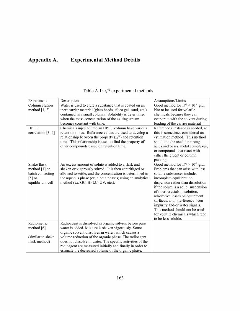
163

Appendix A. Experimental Method Details

Table A.1: xiaq experimental methods

Experiment Description Assumptions/Limits Column elution method [1, 2]

Water is used to elute a substance that is coated on an inert carrier material (glass beads, silica gel, sand, etc.) contained in a small column. Solubility is determined when the mass concentration of the exiting stream becomes constant with time.

Good method for xiaq < 10-2 g/L.

Not to be used for volatile chemicals because they can evaporate with the solvent during loading of the carrier material

HPLC correlation [3, 4]

Chemicals injected into an HPLC column have various retention times. Reference values are used to develop a relationship between the property (xi

aq) and retention time. This relationship is used to find the property of other compounds based on retention time.

Reference substance is needed, so this is sometimes considered an estimation method. This method should not be used for strong acids and bases, metal complexes, or compounds that react with either the eluent or column packing.

Shake flask method [1] or batch contacting [5] or equilibrium cell

An excess amount of solute is added to a flask and shaken or vigorously stirred. It is then centrifuged or allowed to settle, and the concentration is determined in the aqueous phase (or in both phases) using an analytical method (ex. GC, HPLC, UV, etc.).

Good method for xiaq > 10-2 g/L.

Problems that can arise with less soluble substances include: incomplete equilibration, dispersion rather than dissolution if the solute is a solid, suspension of microcrystals in solution, adsorptive losses on equipment surfaces, and interference from impurity and/or water signals. This method should not be used for volatile chemicals which tend to be less soluble.

Radiometric method [6] (similar to shake flask method)

Radioagent is dissolved in organic solvent before pure water is added. Mixture is shaken vigorously. Some organic solvent dissolves in water, which causes a volume reduction of the organic phase. The radioagent does not dissolve in water. The specific activities of the radioagent are measured initially and finally in order to estimate the decreased volume of the organic phase.

164

Table A.1: xiaq experimental methods

Experiment Description Assumptions/Limits Generator column or dynamic coupled column liquid chromatographic technique [7-12]

Water is pumped through the generator column that is packed with a solid support coated with the test compound to produce a saturated aqueous solution. The compound is then extracted from the saturated solution onto an extractor column. It is then eluted with a solvent/water mixture and analyzed with HPLC or GC. The water solubility is the concentration of the compound in the generator column effluent. (similar to column elution method)

This method avoids errors that could result from sorption on glassware and the presence of colloids when measuring small concentrations. Recommended range is 1 ppb-500 ppm.

Nephelometric or turbidity method [13]

Several dilutions are made of a stable suspension of known concentration. A plot of concentration verses turbidity produces a line. xi

aq is the concentration at 0 turbidity, and it can be estimated through a linear regression of the turbidity data.

This method cannot distinguish between solute and impurities. Recommended for xi

aq > 10-3 g/L if the solute forms stable suspensions in water.

Slow stir method [13]

The sample is dissolved in a volatile solvent. This solution is deposited on the walls (not the bottom) of a glass container, and the solvent is evaporated using nitrogen. Water and a magnetic stir bar are added, and the system is mixed until equilibrium is reached. The concentration in the aqueous phase is then determined using an appropriate analytical technique.

Recommended for xiaq < 10-3 g/L.

This method avoids emulsions.

Gas solubility methods

The apparatus is a complex system that uses manometers and multiple vessels. A known mass of solvent is used. Equilibration can be accomplished through stirring, bubbling, shaking, or static contact. The final concentration can be determined by mass, pressure, volume, or an analytical technique.

Thermostatic (for SOLC) [14]

In various solvents, the solubility of silver perchlorate increases in the presence of trace amounts of water. The solubility behavior can be used to determine how much water is present.

Vapor Saturation [15]

Solvent is equilibrated with solute vapor.

Residue volume or volumetric method or absorbed volume [16, 17]

An excess of solute is added and the mixture is centrifuged. The residue of solute is then measured volumetrically. The data is then plotted as grams of solute added vs. volume of undissolved residue. The value at zero volume of undissolved residue is then extrapolated.

Synthetic method [17]

Weighed quantities of solute and solvent are sealed up together. The temperature at which turbidity appears/disappears is determined in a temperature bath.

This cannot distinguish between solute and impurities.

Multiple equilibration [18]

See Table A.2 for description.

Dialysis tubing method [19]

Dialysis tubing containing pure water is knotted on one end, connected to glass tubing on the other end, and sealed with a plastic cap. This tubing is then put in a test tube containing solute. Injections are taken and analyzed with a GC.

(cont.)

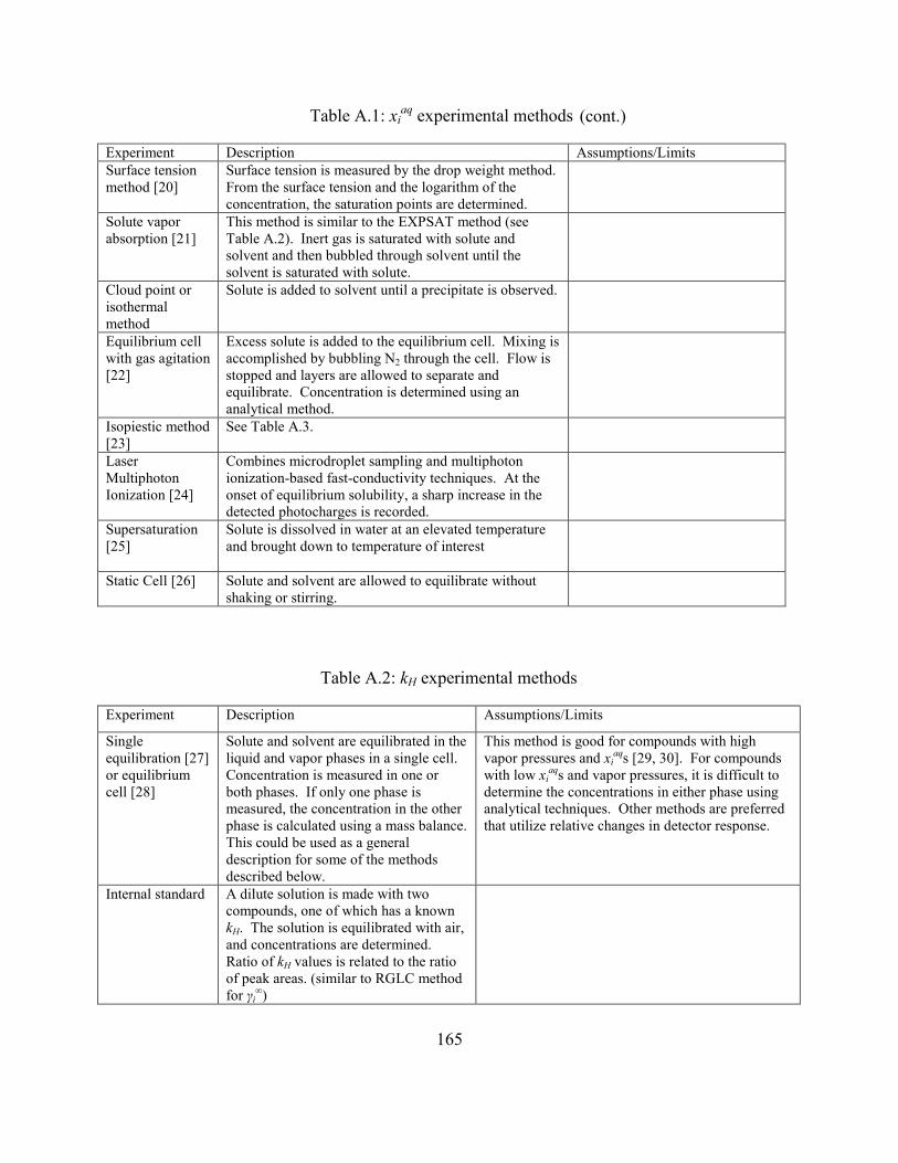
165

Table A.1: xiaq experimental methods

Experiment Description Assumptions/Limits Surface tension method [20]

Surface tension is measured by the drop weight method. From the surface tension and the logarithm of the concentration, the saturation points are determined.

Solute vapor absorption [21]

This method is similar to the EXPSAT method (see Table A.2). Inert gas is saturated with solute and solvent and then bubbled through solvent until the solvent is saturated with solute.

Cloud point or isothermal method

Solute is added to solvent until a precipitate is observed.

Equilibrium cell with gas agitation [22]

Excess solute is added to the equilibrium cell. Mixing is accomplished by bubbling N2 through the cell. Flow is stopped and layers are allowed to separate and equilibrate. Concentration is determined using an analytical method.

Isopiestic method [23]

See Table A.3.

Laser Multiphoton Ionization [24]

Combines microdroplet sampling and multiphoton ionization-based fast-conductivity techniques. At the onset of equilibrium solubility, a sharp increase in the detected photocharges is recorded.

Supersaturation [25]

Solute is dissolved in water at an elevated temperature and brought down to temperature of interest

Static Cell [26] Solute and solvent are allowed to equilibrate without shaking or stirring.

Table A.2: kH experimental methods

Experiment Description Assumptions/Limits

Single equilibration [27] or equilibrium cell [28]

Solute and solvent are equilibrated in the liquid and vapor phases in a single cell. Concentration is measured in one or both phases. If only one phase is measured, the concentration in the other phase is calculated using a mass balance. This could be used as a general description for some of the methods described below.

This method is good for compounds with high vapor pressures and xi

aqs [29, 30]. For compounds with low xi

aqs and vapor pressures, it is difficult to determine the concentrations in either phase using analytical techniques. Other methods are preferred that utilize relative changes in detector response.

Internal standard A dilute solution is made with two compounds, one of which has a known kH. The solution is equilibrated with air, and concentrations are determined. Ratio of kH values is related to the ratio of peak areas. (similar to RGLC method for γi

∞)

(cont.)

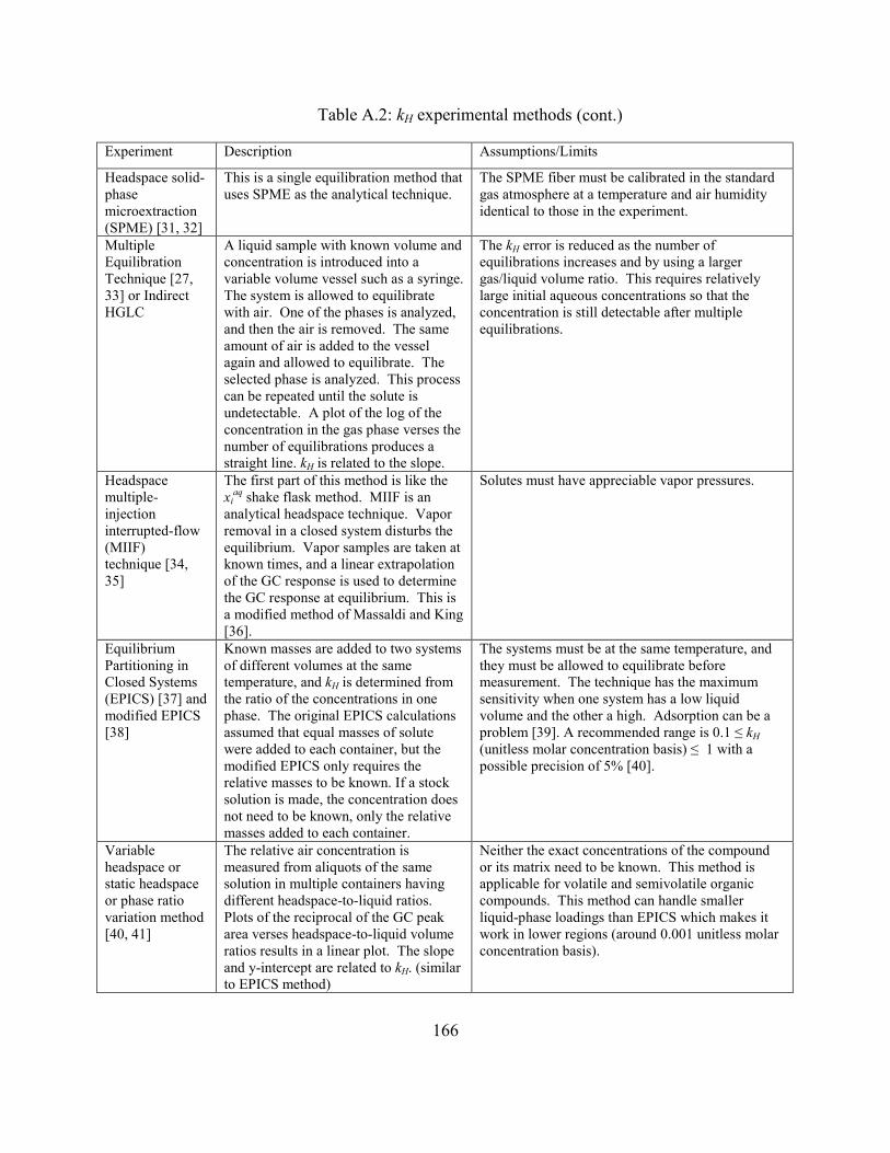
166

Table A.2: kH experimental methods

Experiment Description Assumptions/Limits

Headspace solid-phase microextraction (SPME) [31, 32]

This is a single equilibration method that uses SPME as the analytical technique.

The SPME fiber must be calibrated in the standard gas atmosphere at a temperature and air humidity identical to those in the experiment.

Multiple Equilibration Technique [27, 33] or Indirect HGLC

A liquid sample with known volume and concentration is introduced into a variable volume vessel such as a syringe. The system is allowed to equilibrate with air. One of the phases is analyzed, and then the air is removed. The same amount of air is added to the vessel again and allowed to equilibrate. The selected phase is analyzed. This process can be repeated until the solute is undetectable. A plot of the log of the concentration in the gas phase verses the number of equilibrations produces a straight line. kH is related to the slope.

The kH error is reduced as the number of equilibrations increases and by using a larger gas/liquid volume ratio. This requires relatively large initial aqueous concentrations so that the concentration is still detectable after multiple equilibrations.

Headspace multiple-injection interrupted-flow (MIIF) technique [34, 35]

The first part of this method is like the xi

aq shake flask method. MIIF is an analytical headspace technique. Vapor removal in a closed system disturbs the equilibrium. Vapor samples are taken at known times, and a linear extrapolation of the GC response is used to determine the GC response at equilibrium. This is a modified method of Massaldi and King [36].

Solutes must have appreciable vapor pressures.

Equilibrium Partitioning in Closed Systems (EPICS) [37] and modified EPICS [38]

Known masses are added to two systems of different volumes at the same temperature, and kH is determined from the ratio of the concentrations in one phase. The original EPICS calculations assumed that equal masses of solute were added to each container, but the modified EPICS only requires the relative masses to be known. If a stock solution is made, the concentration does not need to be known, only the relative masses added to each container.

The systems must be at the same temperature, and they must be allowed to equilibrate before measurement. The technique has the maximum sensitivity when one system has a low liquid volume and the other a high. Adsorption can be a problem [39]. A recommended range is 0.1 ≤ kH (unitless molar concentration basis) ≤ 1 with a possible precision of 5% [40].

Variable headspace or static headspace or phase ratio variation method [40, 41]

The relative air concentration is measured from aliquots of the same solution in multiple containers having different headspace-to-liquid ratios. Plots of the reciprocal of the GC peak area verses headspace-to-liquid volume ratios results in a linear plot. The slope and y-intercept are related to kH. (similar to EPICS method)

Neither the exact concentrations of the compound or its matrix need to be known. This method is applicable for volatile and semivolatile organic compounds. This method can handle smaller liquid-phase loadings than EPICS which makes it work in lower regions (around 0.001 unitless molar concentration basis).

(cont.)

167

Table A.2: kH experimental methods

Experiment Description Assumptions/Limits

Batch air stripping [30] or inert gas stripping or gas stripping or air stripping or exponential dilutor method

A dilute solution is stripped using an inert gas (usually N2). The change in concentration with time is related to kH. Some experiments first saturate the stripping gas with water. There are many variations of this method. The original equation has been expanded upon by multiple authors to include various corrections. Some authors take into account different corrections while others do not.

When compared to the single equilibration method, adsorption is less likely to be an issue due to the dynamic principle and turbulent conditions [39]. Absolute detector response is unimportant; it just needs to be linear [42]. It can be difficult to determine if equilibrium is reached [37] . The depth/height of the column can be increased. If the value does not change, then equilibrium was reached. However, a taller tower makes it harder to ensure complete mixing. Equilibrium can be verified by changing the flow rate of the stripping gas and seeing if kH remains constant [43]. A range of system volumes and purge gas flow rates can also be used to verify the assumptions of complete mixing and equilibrium [44]. Non-equilibrium leads to biased results [27, 39]. This method works for chemicals with low solubilities and vapor pressures [29, 45], but problems can arise if the volatility is too low because it is difficult to detect a change in concentration after air stripping [44]. It is a good method for systems with a high limiting relative volatility and involatile solvents [46]. Bias has been reported for this method for semivolatile organic chemicals[47]. The authors claim there can be significant absorption on the surface of the bubbles. When they pop on the surface, they release excess chemical into the headspace. Recommended ranges are 0.0001 < kH (unitless molar concentration basis) <1[31]; relative volatility > 1000 [48]; 10 kPa < kH <105 kPa and P2

sat < 50 kPa [40] with 1% uncertainty possible in this range. The diameter of the bubble should be below 1 mm, and they should not coalesce [40, 49] A good relative elution rate is 0.01 min-1 or lower. Minimize the vapor space, and use as dilute a solution as possible.

EXPSAT (exponential saturator)[50, 51]

Contaminated air/N2 (gas first saturated with solute) is bubbled through water to resemble what happens in atmosphere.

An advantage over gas stripping is that dissolution of hydrophobic compound in water to make dilute solution is not required [40]. Recommended ranges: 500 < γi

∞ < 105 or 1 MPa < kH < 100 MPa with precision possible of 1-2%.

Modified gas stripping[52]

Differences between this and inert gas stripping are that chemical is introduced into stripping cell using a separate loop. Solute is in a separate flask. The line between the flask and stripping cell is “vacuumed”. Line is opened and water saturated carrier is used to carry solute into cell (similar idea to EXPSAT). The concentration is monitored real time.

This is faster than the inert gas stripping method. This can be applied to a broader range of compounds than normal gas stripping.

(cont.)

168

Table A.2: kH experimental methods

Experiment Description Assumptions/Limits

Purge and trap[53] or gas sparging [54] or dynamic equilibrium system [55]

An inert gas is bubbled through a purge chamber. The exiting solute is deposited on a cooled trap or cartridge. The trap is then heated in order to inject the solute into the GC or solute can be extracted from the cartridge with solvent in order to inject into the GC.

Packed column [56]

Similar to the inert gas stripping method. Column just has packing in it.

Packing eliminates problem of aerosols/bursting bubbles at surface

Counterflow packed column[56, 57]

Water-saturated air flows up through a packed column. The test solution flows down through the column. The exiting solution is collected and analyzed for concentration.

This can be used for compounds with low to moderate volatilities. Recommended range is 1∙10-4 ≤ kH (unitless molar concentration basis) ≤ 5∙10-2. The stripping factor must be less than 1. If the stripping factor is too small, it can be difficult to measure differences between inlet and outlet concentration.

Concurrent flow or wetted wall column [58, 59]

Solute-saturated water enters the wetted-wall column where it is in contact with a concurrent flow of gas (air). The two streams are separated at the bottom of the column and analyzed using GC.

The system must be validated to ensure full equilibrium is reached within the column [27].

Horizontal Flow Reactor [60]

This method is a cross between the wetted wall column method and evaporation from a water surface. N2 is blown through a horiztonal tube. A container of water is sitting stagnant on the bottom of the tube.

Evaporation from a water surface [61]

Air is blown across the top of a solution at a known flow rate to evaporate the solute. The concentrations of solute in the water and gas phases are measured. Equilibrium is not achieved, so estimated mass transfer coefficients are used to determine the departure from equilibrium.

This method is for substances with low air-water partition coefficients that aggregate in solution, ionize, or display surface activity. Recommended range is kH (unitless molar concentration basis) < 10-3.

Diffusion in air and water boundary layers [62]

kH is obtained from two partition coefficients between polydimetholsiloxane (PDMS) and air and between PDMS and water. Partition coefficients with PDMS are determined by measuring the mass transfer rate constants in the boundary layer.

(cont.)

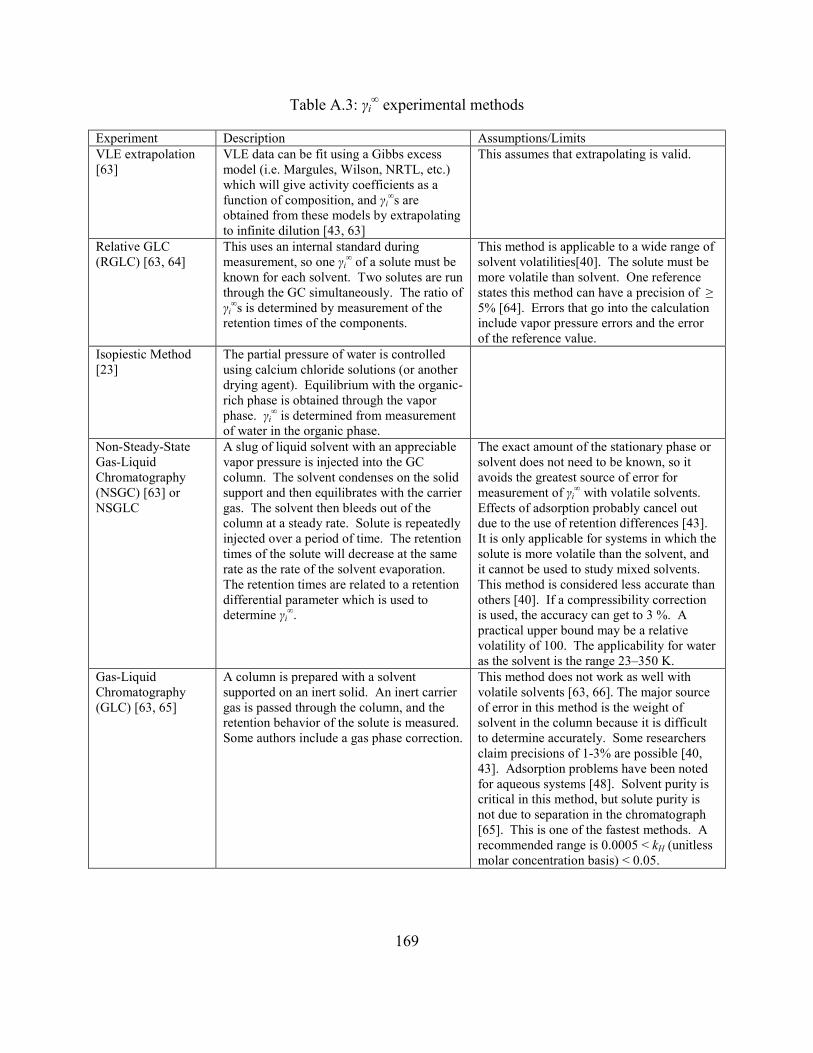
169

Table A.3: γi∞ experimental methods

Experiment Description Assumptions/Limits VLE extrapolation [63]

VLE data can be fit using a Gibbs excess model (i.e. Margules, Wilson, NRTL, etc.) which will give activity coefficients as a function of composition, and γi

∞s are obtained from these models by extrapolating to infinite dilution [43, 63]

This assumes that extrapolating is valid.

Relative GLC (RGLC) [63, 64]

This uses an internal standard during measurement, so one γi

∞ of a solute must be known for each solvent. Two solutes are run through the GC simultaneously. The ratio of γi

∞s is determined by measurement of the retention times of the components.

This method is applicable to a wide range of solvent volatilities[40]. The solute must be more volatile than solvent. One reference states this method can have a precision of ≥ 5% [64]. Errors that go into the calculation include vapor pressure errors and the error of the reference value.

Isopiestic Method [23]

The partial pressure of water is controlled using calcium chloride solutions (or another drying agent). Equilibrium with the organic-rich phase is obtained through the vapor phase. γi

∞ is determined from measurement of water in the organic phase.

Non-Steady-State Gas-Liquid Chromatography (NSGC) [63] or NSGLC

A slug of liquid solvent with an appreciable vapor pressure is injected into the GC column. The solvent condenses on the solid support and then equilibrates with the carrier gas. The solvent then bleeds out of the column at a steady rate. Solute is repeatedly injected over a period of time. The retention times of the solute will decrease at the same rate as the rate of the solvent evaporation. The retention times are related to a retention differential parameter which is used to determine γi

∞.

The exact amount of the stationary phase or solvent does not need to be known, so it avoids the greatest source of error for measurement of γi

∞ with volatile solvents. Effects of adsorption probably cancel out due to the use of retention differences [43]. It is only applicable for systems in which the solute is more volatile than the solvent, and it cannot be used to study mixed solvents. This method is considered less accurate than others [40]. If a compressibility correction is used, the accuracy can get to 3 %. A practical upper bound may be a relative volatility of 100. The applicability for water as the solvent is the range 23–350 K.

Gas-Liquid Chromatography (GLC) [63, 65]

A column is prepared with a solvent supported on an inert solid. An inert carrier gas is passed through the column, and the retention behavior of the solute is measured. Some authors include a gas phase correction.

This method does not work as well with volatile solvents [63, 66]. The major source of error in this method is the weight of solvent in the column because it is difficult to determine accurately. Some researchers claim precisions of 1-3% are possible [40, 43]. Adsorption problems have been noted for aqueous systems [48]. Solvent purity is critical in this method, but solute purity is not due to separation in the chromatograph [65]. This is one of the fastest methods. A recommended range is 0.0005 < kH (unitless molar concentration basis) < 0.05.

(cont.)

170

Table A.3: γi∞ experimental methods

Experiment Description Assumptions/Limits Headspace GLC (HGLC) [40, 48, 67]

The headspace above a solution is analyzed using GC and the response is related to γi

∞. The major limitation is the lack of high quality experimental gas phase virial coefficients needed to correct for pressure. A recommended range is 20 < kH (unitless molar concentration basis) < 20,000. For insoluble solutes or low kHs, the RGLC or gas stripping methods are preferred. Under good conditions, HGLC can give precision within 1-5%.

Indirect HGLC [68] Indirect HGLC measures the hexadecane-water partition coefficient and relates it to γi

∞. The solute GC peak area of the vapor phase in equilibrium with a dilute aqueous solution is measured, and then it is measured again after the addition of a known volume of hexadecane. The partition coefficient is determined from the ratio of GC peak areas and the volume of hexadecane which is then related to γi

∞.

This method does not require a standard solution of the solute or calibration of the detector. However, it does require that the air-hexadecane partition coefficient be known. The solute must be volatile enough to be detected in the headspace of the water-hexadecane system.

Liquid-Liquid Chromatography (LLC) [66]

LLC is used to determine the γi∞ ratio of a

solute between a mobile and stationary phase which is a liquid on a solid support. It is necessary to determine γi

∞ of the solute in one of the phases using another technique in order to determine γi

∞ in the other phase.

This method is only accurate if the mutual solubilities of the stationary phase and mobile phase are negligible. The accuracy of this method is not as high as the GC techniques [43]. There have been reported adsorption problems for aqueous systems [48].

Gas stripping See description in Table A.2. EXPSAT method [40]

Exponential saturator method. See description in Table A.2.

Differential distillation [40] or transpiration method

A small amount of solute is distilled off (using an inert gas) of a dilution solution so that its composition is essentially unchanged. Concentrations of samples in the distillate and batch solution are determined.

This is recommended for relative volatilites << 1. Relatively large batches of solution are required, so this is a good method for water and inexpensive solvents.

Differential Ebulliometry [69]

Differential ebulliometry consists of measuring the difference in boiling points of a pure solvent and the solvent with dissolved solute [70]. The data can be related back to the γi

∞ through thermodynamics.

Steady state can be achieved fairly quickly [71]; however, steady state may not represent true equilibrium. This method requires characterization of the ebulliometer and accurate determination of the vaporization ratio. Ebulliometry yields accurate results for systems where the limiting relative volatility is near unity [43, 46]. Another recommended range is for relative volatilities between 0.3-20 [48]. The accuracy is not as good for high-boiling-point systems and highly viscous systems [43].

(cont.)

171

Table A.3: γi∞ experimental methods

Experiment Description Assumptions/Limits Rayleigh distillation method [40, 46] (similar to differential distillation)

It is based on a single stage distillation. A dilute solution is prepared in a glass equilibrium cell. An inert gas is introduced into the solution at a flow rate that will ensure complete saturation. When enough solution has been distilled off, the cell is weighed, and the solution is analyzed using chromatography. The GC peak response and mass ratios are related to γi

∞.

Dilute solutions must be used. This method can reach precision of 1%. A flow rate of about 0.2 cm3/s is required for aqueous solutions. A recommended range for relative volatilities is 1-70.

Differential static cell method [43, 72]

The differences in equilibrium vapor pressure are measured at constant temperature between a dilute solution and the pure solvent as a function of composition in the dilute solution. For solutes with similar volatility as water, liquid composition is determined gravimetrically. Since composition is not measured directly, a vaporization correction must be made for volatile solutes since they vaporize into the headspace.

This method has been applied to measure solubility without a compositional analysis. A correction must be made to measured data, but this method is better than others (such as ebulliometry) for solvents with poor boiling properties (such as water or polymer solutions) or for mixtures with high relative volatility.

Circulation Still [40, 73]

VLE circulation still operated at constant pressure used to provide samples of corresponding vapor and liquid compositions. No measurement of temperature needed as the boiling temp of the solution is indistinguishable from that of the neat solvent.

Recommended ranges are 30 K below the normal boiling temperature of the solvent and a relative volatility between 0.1-30. An uncertainty of 3-5% is possible.

Dew-point method [43, 72, 74]

The dew point method is similar to the ebulliometric method. The change in dew temperature of the vapor of a solvent is measured as a small amount of solute is added.

This method works well for systems with relative volatilities below about 0.3. GLC, GS, HGLC, ebulliometry, and the differential static methods all have difficulties measuring γi

∞ at volatilities this low. This method is typically limited to binary systems of low volatility.

Molecular Beams [75]

The vapors from each of two vapor-liquid equilibrium cells are collimated into molecular beams. The beams are alternately chopped before being detected by a mass spectrometer. The output signal from the mass spectrometer will be representative of the difference in partial pressure for any component in the two cells. Differences in pressure between apure component and that containing a species at infinite dilution can be easily detected.

(cont.) (cont.)

172

Table A.4: KOW experimental methods

Experiment Description Assumptions/Limits Shake flask method [45, 76, 77]

Solute is added to a flask with octanol/water and shaken. The concentrations are determined in the phases using an analytical method.

The recommend range is approximately -2 ≥ logKOW ≥ 4. This method should typically not be used for polycyclic aromatic substances without polar substituents; halogenated hydrocarbons; or large, non-polar chemicals.

Generator column [78]

A generator column is packed with a support that is coated in the test chemical at a fixed n-octanol concentration. The solute is eluted from the column with water. The extractor column extracts solute from the aqueous phase, and it is then eluted and analyzed using HPLC or GC.

This can be used for 1 < logKOW < 6.

Slow stir method [45, 79]

This method is similar to the shake flask method. The main difference is that the octanol and water phases are slowly stirred instead of shaken while the system reaches equilibrium.

This method prevents the formation of emulsions. It can be used for 5 < logKOW < 8.2.

HPLC correlation (indirect) [3, 80, 81]

Chemicals injected into an HPLC column have various retention times. Reference values are used to develop a relationship between the property (xi

aq or KOW) and retention time. This equation is used to find the property of other compounds based on retention time.

Reference substances are needed, so this is sometimes considered an estimation method. Recommended ranges are 0 < logKOW < 6 according to OPPTS and OECD and 0 < logKOW < 8 according to ASTM. This method should not be used for strong acids and bases, metal complexes, or compounds that react with either the eluent or column packing.

173

Appendix A References

1. Organisation for Economic Co-operation and Development, OECD Guideline for the Testing of Chemicals: 105 Water Solubility, 1995.

2. U.S. Environmental Protection Agency Office of Prevention Pesticides and Toxic Substances, Product Properties Test Guidelines: OPPTS 830.7840 Water Solubility: Column Elution Method; Shake Flask Method, 1996.

3. Organisation for Economic Co-operation and Development, OECD Guidelines for the Testing of Chemicals: 117 Partition Coefficient (n-octanol/water), High Performance Liquid Chromatography (HPLC) Method, 2004.

4. Chin, Y.P., W.J. Weber, Jr., and T.C. Voice, Determination of partition coefficients and aqueous solubilities by reverse phase chromatography - II. Evaluation of partitioning and solubility models. Water Res., 1986. 20(11): p. 1443-50.

5. Beneš, M. and V. Dohnal, Limiting Activity Coefficients of Some Aromatic and Aliphatic Nitro Compounds in Water. J. Chem. Eng. Data, 1999. 44(5): p. 1097-1102.

6. Lo, J.M., C.L. Tseng, and J.Y. Yang, Radiometric method for determining solubility of organic solvents in water. Anal. Chem., 1986. 58(7): p. 1596-1597.

7. U.S. Environmental Protection Agency Office of Prevention Pesticides and Toxic Substances, Product Properties Test Guidelines: OPPTS 830.7860 Water Solubility (Generator Column Method), 1996.

8. May, W.E., S.P. Wasik, and D.H. Freeman, Determination of the solubility behavior of some polycyclic aromatic hydrocarbons in water. Anal. Chem., 1978. 50(7): p. 997-1000.

9. May, W.E., S.P. Wasik, and D.H. Freeman, Determination of the aqueous solubility of polynuclear aromatic hydrocarbons by a coupled column liquid chromatographic technique. Anal. Chem., 1978. 50(1): p. 175-9.

10. DeVoe, H., M.M. Miller, and S.P. Wasik, Generator columns and high pressure liquid chromatography for determining aqueous solubilities and octanol-water partition coefficients of hydrophobic substances. J. Res. Natl. Bur. Stand. (U. S.), 1981. 86(4): p. 361-6.

11. Wasik, S.P., et al., Octanol/water partition coefficients and aqueous solubilities of organic compounds, 1981, Natl. Bur. Stand.: Washington, D.C. pp. 68.

12. Mackay, D. and W.Y. Shiu, A Critical Review of Henry's Law Constants for Chemicals of Environmental Interest. J. Phys. Chem. Ref. Data, 1981. 10(4): p. 1175-1199.

13. ASTM, E 1148 Standard Test Method for Measurements of Aqueous Solubility, 1987 (1993), ASTM International: West Conshohocken, PA.

14. Hill, A.E., Mutual solubility of liquids. I. Mutual solubility of ethyl ether and water. II. Solubility of water in benzene. J. Am. Chem. Soc., 1923. 45: p. 1143-55.

15. Nelson, H.D. and C.L. de Ligny, The determination of the solubilities of some n-alkanes in water at different temperatures, by means of gas chromatography. Recl. Trav. Chim. Pays-Bas, 1968. 87(5): p. 528-544.

16. Booth, H.S. and H.E. Everson, Hydrotropic Solubilities: Solubilities in 40 Per Cent Sodium Xylenesulfonate. J. Ind. Eng. Chem., 1948. 40(8): p. 1491-1493.

17. Bennett, G.M. and W.G. Philip, Influence of Structure on the Solubilities of Ethers. Part I. Aliphatic Ethers. J. Chem. Soc., 1928: p. 1930-7.

174

18. Mackay, D., W.Y. Shiu, and A.W. Wolkoff, Gas Chromatographic Determination of Low Concentrations of Hydrocarbons in Water by Vapor Phase Extraction. ASTM Special Technical Publication, 1975. 573(Water Quality Parameters Symposium): p. 251-8.

19. Etzweiler, F., E. Senn, and H.W.H. Schmidt, Method for Measuring Aqueous Solubilities of Organic Compounds. Anal. Chem., 1995. 67: p. 655-658.

20. Kinoshita, K., H. Ishikawa, and K. Shinoda, Solubility of Alcohols in Water Determined by the Surface Tension Measurements. Bull. Chem. Soc. Jpn., 1958. 31(9): p. 1081-1082.

21. Dohányosová, P., et al., Measurement of Aqueous Solubility of Hydrophobic Volatile Organic Compounds by Solute Vapor Absorption Technique:  Toluene, Ethylbenzene, Propylbenzene, and Butylbenzene at Temperatures from 273 K to 328 K. J. Chem. Eng. Data, 2001. 46(6): p. 1533-1539.

22. Franks, F., M. Gent, and H.H. Johnson, The Solubility of Benzene in Water. J. Chem. Soc., 1963: p. 2716-2723.

23. Christian, S.D., et al., Control and measurement of water activity. J. Chem. Educ., 1963. 40(8): p. 419-21.

24. Gridin, V.V., et al., Determination of Aqueous Solubility and Surface Adsorption of Polycyclic Aromatic Hydrocarbons by Laser Multiphoton Ionization. Anal. Chem., 1998. 70(13): p. 2685-2692.

25. Chapin, E.M. and J.M. Bell, The Solubility of Oxalic Acid in Aqueous Solutions of Hydrochloric Acid. J. Am. Chem. Soc., 1931. 53: p. 3284-3287.

26. Smith, R.R., N.W. Charon, and W.J. Canady, Thermodynamics of Solution of Aromatic Hydrocarbons in Water and in Water-Ethanol Solutions: Comparison of Some Methodologies. J. Phys. Chem., 1989. 93: p. 5938-5943.

27. Staudinger, J. and P.V. Roberts, A critical review of Henry's law constants for environmental applications. Crit. Rev. Environ. Sci. Technol., 1996. 26(3): p. 205-297.

28. Leighton, D.T. and J.M. Calo, Distribution coefficients of chlorinated hydrocarbons in dilute air-water systems for groundwater contamination applications. J. Chem. Eng. Data, 1981. 26(4): p. 382-385.

29. Alaee, M., R.M. Whittal, and W.M.J. Strachan, The effect of water temperature and composition on Henry's law constant for various PAH's. Chemosphere, 1996. 32(6): p. 1153-1164.

30. Mackay, D., W.Y. Shiu, and R.P. Sutherland, Determination of air-water Henry's law constants for hydrophobic pollutants. Environ. Sci. Technol., 1979. 13(3): p. 333-337.

31. Böhme, A., et al., Determination of Temperature-Dependent Henry's Law Constant of Four Oxygenated Solutes in Water Using Headspace Solid-Phase Microextraction Technique. J. Chem. Eng. Data, 2008. 53(12): p. 2873-2877.

32. Omur-Ozbek, P., Determination of temperature-dependent constants of odorous contaminants and their application to human perception. Environ. Sci. Technol., 2005. 39: p. 3957-3963.

33. McAullife, C., GC [gas-chromatographic] determination of solutes by multiple phase equilibration. Chem. Technol., 1971(Jan.): p. 46-51.

34. Keeley, D.F., M.A. Hoffpauir, and J.R. Meriwether, Solubility of aromatic hydrocarbons in water and sodium chloride solutions of different ionic strengths: benzene and toluene. J. Chem. Eng. Data, 1988. 33(2): p. 87-89.

175

35. Keeley, D.F., M.A. Hoffpauir, and J.R. Meriwether, Solubility of aromatic hydrocarbons in water and sodium chloride solutions of different ionic strengths: C2-Substituted benzenes. J. Chem. Eng. Data, 1991. 36(4): p. 456-459.

36. Massaldi, H.A. and C.J. King, Simple technique to determine solubilities of sparingly soluble organics. Solubility and activity coefficients of d-limonene, butylbenzene, and n-hexyl acetate in water and sucrose solutions. J. Chem. Eng. Data, 1973. 18(4): p. 393-7.

37. Gosset, J.M., et al., Mass transfer coefficients and Henry's constants for packed-tower air stripping of volatile organics: measurements and correlation, 1985, Dep. Civ. Eng.,Cornell Univ., Ithaca, NY, USA. pp. 294.

38. Gossett, J.M., Measurement of Henry's law constants for C1 and C2 chlorinated hydrocarbons. Environ. Sci. Technol., 1987. 21(2): p. 202-8.

39. Nielsen, F., E. Olsen, and A. Fredenslund, Henry's Law Constants and Infinite Dilution Activity Coefficients for Volatile Organic Compounds in Water by a Validated Batch Air Stripping Method. Environ. Sci. Technol., 1994. 28(12): p. 2133-2138.

40. Dohnal, V., Measurement of Limiting Activity Coefficients Using Analytical Tools, in Measurement of the Thermodynamic Properties of Multiple Phases, R.D. Weir and T.W.d. Loos, Editors. 2005, Elsevier: Amsterdam. p. 359-381.

41. Robbins, G.A., S. Wang, and J.D. Stuart, Using the static headspace method to determine Henry's law constants. Anal. Chem., 1993. 65(21): p. 3113-18.

42. Li, J., et al., Measurement of large infinite dilution activity coefficients of nonelectrolytes in water by inert gas stripping and gas chromatography. Anal. Chem., 1993. 65(22): p. 3212-3218.

43. Kojima, K., S. Zhang, and T. Hiaki, Measuring methods of infinite dilution activity coefficients and a database for systems including water. Fluid Phase Equilib., 1997. 131(1-2): p. 145-179.

44. Gossett, J.M. and A.H. Lincoff, Solute-gas equilibriums in multi-organic aqueous systems, 1981, Dep. Environ. Eng., Cornell Univ., Ithaca, NY, USA. pp. 37.

45. U.S. Environmental Protection Agency, Chemistry Assistance Manual for Premanufacture Notification Submitters, 1997.

46. Dohnal, V. and I. Horakova, A new variant of the Rayleigh distillation method for the determination of limiting activity coefficients. Fluid Phase Equilib., 1991. 68: p. 173-85.

47. Shunthirasingham, C., Y.D. Lei, and F. Wania, Evidence of Bias in Air−Water Henry's Law Constants for Semivolatile Organic Compounds Measured by Inert Gas Stripping. Environ. Sci. Technol., 2007. 41(11): p. 3807-3814.

48. Sherman, S.R., et al., Compilation and Correlation of Limiting Activity Coefficients of Nonelectrolytes in Water. Ind. Eng. Chem. Res., 1996. 35(4): p. 1044-58.

49. Richon, D., P. Antoine, and H. Renon, Infinite dilution activity coefficients of linear and branched alkanes from C1 to C9 in n-hexadecane by inert gas stripping. Ind. Eng. Chem. Process Des. Dev., 1980. 19(1): p. 144-7.

50. Kames, J., S. Schweighoefer, and U. Schurath, Henry's Law constant and hydrolysis of peroxyacetyl nitrate (PAN). J. Atmos. Chem., 1991. 12(2): p. 169-80.

51. Dohnal, V. and S. Hovorka, Exponential Saturator: A Novel Gas-Liquid Partitioning Technique for Measurement of Large Limiting Activity Coefficients. Ind. Eng. Chem. Res., 1999. 38(5): p. 2036-2043.

176

52. Richon, D., New equipment and new technique for measuring activity coefficients and Henry's constants at infinite dilution. Rev. Sci. Instrum., 2011. 82(2): p. 025108/1-025108/8.

53. Ruiz-Bevia, F. and M.J. Fernandez-Torres, Determining the Henry's Law constants of THMs in seawater by means of purge-and-trap gas chromatography (PT-GC): the influence of seawater as sample matrix. Anal. Sci., 2010. 26(6): p. 723-6.

54. Dacey, J.W.H., S.G. Wakeham, and B.L. Howes, Henry's law constants for dimethylsulfide in freshwater and seawater. Geophys. Res. Lett., 1984. 11(10): p. 991-994.

55. Poulain, L., et al., In-cloud multiphase behaviour of acetone in the troposphere: gas uptake, Henry's law equilibrium and aqueous phase photooxidation. Chemosphere, 2010. 81(3): p. 312-20.

56. Johnson, B.J., E.A. Betterton, and D. Craig, Henry's law coefficient of formic and acetic acids. J. Atmos. Chem., 1996. 24(2): p. 113-119.

57. Caires, J.P., M. Suzuki, and T.C.G. Kibbey, Counterflow Method for Measurement of Henry's Law Constants. J. Environ. Eng., 2003. 129: p. 1169-1175.

58. Fendinger, N.J. and D.E. Glotfelty, A laboratory method for the experimental determination of air-water Henry's law constants for several pesticides. Environ. Sci. Technol., 1988. 22(11): p. 1289-93.

59. Emmert, R.E. and R.L. Pigford, Interfacial resistance. A study of gas absorption in falling liquid films. Chem. Eng. Prog., 1954. 50: p. 87-93.

60. Strekowski, R.S. and C. George, Measurement of Henry's Law Constants for Acetone, 2-Butanone, 2,3-Butanedione, and Isobutyraldehyde Using a Horizontal Flow Reactor. J. Chem. Eng. Data, 2005. 50(3): p. 804-810.

61. Li, H., D. Ellis, and D. Mackay, Measurement of low air-water partition coefficients of organic acids by evaporation from a water surface. J. Chem. Eng. Data, 2007. 52(5): p. 1580-1584.

62. Lee, H., H.-J. Kim, and J.-H. Kwon, Determination of Henry's Law Constant Using Diffusion in Air and Water Boundary Layers. J. Chem. Eng. Data, 2012. 57(11): p. 3296-3302.

63. Activity coefficients at infinite dilution, ed. D. Tiegs. 1986, Frankfurt/Main : Great Neck, N.Y.: Frankfurt/Main : DECHEMA ; Great Neck, N.Y. : Distributed by Scholium International.

64. Orbey, H. and S.I. Sandler, Relative measurements of activity coefficients at infinite dilution by gas chromatography. Ind. Eng. Chem. Res., 1991. 30(8): p. 2006-11.

65. Thomas, E.R., et al., Limiting activity coefficients of nonpolar and polar solutes in both volatile and nonvolatile solvents by gas chromatography. J. Chem. Eng. Data, 1982. 27(4): p. 399-405.

66. Alessi, P. and I. Kikic, Activity coefficients determination by liquid-liquid chromatography. Gazz. Chim. Ital., 1974. 104(7-8): p. 739-46.

67. Hussam, A. and P.W. Carr, Rapid and precise method for the measurement of vapor/liquid equilibria by headspace gas chromatography. Anal. Chem., 1985. 57(4): p. 793-801.

177

68. Li, J. and P.W. Carr, Measurement of water-hexadecane partition coefficients by headspace gas chromatography and calculation of limiting activity coefficients in water. Anal. Chem., 1993. 65(10): p. 1443-50.

69. Bernauer, M. and V. Dohnal, Temperature Dependence of Air-Water Partitioning of N-Methylated (C1 and C2) Fatty Acid Amides. J. Chem. Eng. Data, 2008. 53(11): p. 2622-2631.

70. Moore, R.C., Henry's Law Constant for Environmentally Significant Compounds. Appl. Biochem. Biotechnol., 1992. 34-5: p. 671-680.

71. Raal, J.D. and D. Ramjugernath, Measurement of Limiting Activity Coefficients: Non-Analytical Tools, in Measurement of the Thermodynamic Properties of Multiple Phases, R.D. Weir and T.W.d. Loos, Editors. 2005, Elsevier: Amsterdam. p. 339-357.

72. Wright, D.A., S.I. Sandler, and D. DeVoll, Infinite dilution activity coefficients and solubilities of halogenated hydrocarbons in water at ambient temperatures. Environ. Sci. Technol., 1992. 26(9): p. 1828-1831.

73. Ondo, D. and V. Dohnal, Temperature dependence of limiting activity coefficients and Henry's law constants of cyclic and open-chain ethers in water. Fluid Phase Equilib., 2007. 262(1-2): p. 121-136.

74. Trampe, D.B. and C.A. Eckert, A dew point technique for limiting activity coefficients in nonionic solutions. AIChE J., 1993. 39(6): p. 1045-50.

75. Schmidt, T.W., Determination of infinite dilution activity coefficients (γ∞) using molecular beams, 1980, Phillips Petroleum Co.: United States.

76. U.S. Environmental Protection Agency Office of Prevention Pesticides and Toxic Substances, Product Properties Test Guidelines: OPPTS 830.7550 Partition Coefficient (n-Octanol/Water), Shake Flask Method, 1996.

77. Organisation for Economic Co-operation and Development, OECD Guidelines for the Testing of Chemicals: 107 Partition Coefficient (n-octanol/water): Shake Flask Method, 1995.

78. U.S. Environmental Protection Agency Office of Prevention Pesticides and Toxic Substances, Product Properties Test Guidelines: OPPTS 830.7560 Partition Coefficient (n-Octanol/Water), Generator Column Method, 1996.

79. Organisation for Economic Co-operation and Development, OECD Guidelines for the Testing of Chemicals: 123 Partition Coefficient (1-Octanol/Water): Slow-Stirring Method, 2006.

80. U.S. Environmental Protection Agency Office of Prevention Pesticides and Toxic Substances, Product Properties Test Guidelines: OPPTS 830.7570 Partition Coefficient (n-Octanol/Water), Estimation By Liquid Chromatography, 1996.

81. Veith, G.D. and R.T. Morris, A Rapid Method for Estimating Log P, 1978: Duluth, MN.

179

Appendix B. Fugacity Error Propagation

The total error of a function can be determined by taking the partial derivatives of the

function with respect to all of the variables. In general terms, y is a function of a, b, c, etc.,

,...),,( cbafy = .

The variance in y, sy, can be determined using the partial derivatives of the function with respect

to all of the variables (a, b, c, etc.) and the variances of the variables (sa, sb, sc, etc.)

...22

22

22

2 +

∂∂

+

∂∂

+

∂∂

= cbay scxs

bxs

axs .

The error associated with the fugacity ratio,Ψ, must be estimated in order to determine the

uncertainty of γi∞. The natural log of equation 4.15 yields

( ) dTRT

dTCpdTCpHT

Tm

T

Tm

Si

T

Tm

LiTmf

i

i

ii∫∫∫ −+∆

=Ψ 2

,

ln .

Separating the terms yields:

( ) dTRT

dTCpdT

RT

dTCpdT

RTH T

Tm

T

Tm

SiT

Tm

T

Tm

LiT

Tm

Tmfi

i

i

i

i

i

∫∫

∫∫

∫ −+∆

=Ψ 222,ln .

In order to simplify the error estimation, it has been assumed that Cps are constant and that the

180

error in Tmi is negligible (this was not assumed in the actual calculation). Integrating and

combining terms yields:

( )

+−

−+

−+

+

−

∆−=Ψ 1ln1ln11ln ,

TTm

TmT

RCp

TTm

TmT

RCp

TmTRH i

i

Sii

i

Li

i

Tmfi

.

Due to the assumptions made, the error in ln(Ψi) is determined from:

22

22

2,

2

,ln

lnlnlnSL CpS

i

iCpL

i

iTmHf

Tmf

i sCp

sCp

sH

s

∂Ψ∂

+

∂Ψ∂

+

∆∂Ψ∂

= ∆Ψ ,

where

−−=

∆∂Ψ∂

iTmf

i

TmTRH111ln

,

,

−+

=

∂Ψ∂

1ln1lnT

TmTmT

RCpi

iLi

i ,

and

+−

−=

∂Ψ∂

1ln1lnT

TmTmT

RCpi

iSi

i .

The uncertainties for the individual properties were the uncertainties assigned in DIPPR® 801.

181

Appendix C. Summary of Recommended Values

The regression coefficients determined in this study are included in this appendix.

Coefficients are not included for the API recommendations that were accepted in this study.

Abbreviations used throughout the tables are explained in Table C.1.

Table C.1: Abbreviations used in regression tables

Abbreviation Explanation D Data Type E Experimental

EP Experimental and Predicted P Predicted S Smoothed s Uncertainty of regression

Tmin Minimum temperature of regression (K) Tmax Maximum temperature of regression (K)

U Unknown

The compounds within each table are sorted by chemical family. The DIPPR® equation number

(Eq) is included for each set of coefficients (see Table 4.3). DIPPR® equation 100 was also used

for “regressions” that are only valid at one temperature:

432 ETDTCTBTAY ++++= .

In these instances, only coefficient “A” was defined.

182

Table C.2: kH regression summary (cont.)

Name CAS Eq A B C D E Tmin Tmax s DT 1-ALKENES

1-PENTENE 109-67-1 100 1.867E+06 0 0 0 0 298.15 298.15 < 25% S 1-HEXENE 592-41-6 100 2.190E+06 0 0 0 0 298.15 298.15 < 25% S 1-HEPTENE 592-76-7 100 2.828E+06 0 0 0 0 298.15 298.15 < 10% S 1-OCTENE 111-66-0 100 3.555E+06 0 0 0 0 298.15 298.15 < 10% S 1-NONENE 124-11-8 100 4.854E+06 0 0 0 0 298.15 298.15 < 25% S 1-DECENE 872-05-9 100 6.459E+06 0 0 0 0 298.15 298.15 < 25% P

1-UNDECENE 872-05-9 100 8.669E+06 -1.003E+04 -3.126E+01 0 0 298.15 298.15 < 25% P 1-DODECENE 872-05-9 100 1.108E+07 -5.042E+04 -2.173E+02 2.501E-01 1 298.15 298.15 < 25% P 1-TRIDECENE 592-41-6 100 1.513E+07 -1.203E+04 -3.844E+01 0 0 298.15 298.15 < 50% P

1-TETRADECENE 872-05-9 100 1.827E+07 0 0 0 0 298.15 298.15 < 50% P 1-PENTADECENE 13360-61-7 100 2.493E+07 0 0 0 0 298.15 298.15 < 50% S

2,3,4-ALKENES cis-2-PENTENE 627-20-3 100 1.262E+06 0 0 0 0 298.15 298.15 < 5% E

trans-2-PENTENE 646-04-8 100 1.293E+06 0 0 0 0 298.15 298.15 < 5% E cis-2-HEPTENE 6443-92-1 100 2.341E+06 0 0 0 0 298.15 298.15 < 10% E

trans-2-HEPTENE 14686-13-6 100 2.292E+06 0 0 0 0 298.15 298.15 < 10% E ACETATES

METHYL ACETATE 79-20-9 101 4.579E+02 -2.509E+04 -6.446E+01 0 0 293.15 343.25 < 10% E ETHYL ACETATE 141-78-6 101 2.419E+02 -1.524E+04 -3.230E+01 0 0 288.15 353.15 < 10% E

n-PROPYL ACETATE 109-60-4 101 2.912E+02 -1.778E+04 -3.939E+01 0 0 298 343.25 < 10% E n-BUTYL ACETATE 123-86-4 101 2.499E+02 -1.619E+04 -3.305E+01 0 0 273.15 363.65 < 10% E

ISOBUTYL ACETATE 110-19-0 101 8.284E+01 -8.464E+03 -8.209E+00 0 0 273.15 323.15 < 25% E ISOPENTYL ACETATE 123-92-2 101 3.240E+02 -1.974E+04 -4.386E+01 0 0 273.15 363.85 < 10% E

183

Table C.2: kH regression summary (cont.)

Name CAS Eq A B C D E Tmin Tmax s DT ISOPROPYL ACETATE 108-21-4 101 -6.279E+01 -2.050E+03 1.353E+01 0 0 273.15 310.2 < 25% E sec-BUTYL ACETATE 105-46-4 101 2.287E+02 -1.494E+04 -2.998E+01 0 0 273.15 363.65 < 10% E

VINYL ACETATE 108-05-4 101 1.816E+02 -1.163E+04 -2.364E+01 0 0 273.35 333.15 < 3% E n-PENTYL ACETATE 628-63-7 101 4.256E+02 -2.473E+04 -5.879E+01 0 0 273.15 364.5 < 25% E n-HEXYL ACETATE 142-92-7 101 4.425E+02 -2.542E+04 -6.131E+01 0 0 273.15 363.35 < 25% E n-HEPTYL ACETATE 112-06-1 101 3.811E+03 1.191E+02 0 0 0 298.15 298.15 < 25% P n-OCTYL ACETATE 112-14-1 101 5.471E+03 -1.036E+04 -3.420E+01 0 0 298.15 298.15 < 25% P

tert-BUTYL ACETATE 540-88-5 101 2.451E+02 -1.574E+04 -3.227E+01 0 0 273.15 353.65 < 10% E CYCLOHEXYL ACETATE 622-45-7 101 2.617E+02 -1.729E+04 -3.465E+01 0 0 273.15 363.45 < 10% E

PHENYL ACETATE 122-79-2 101 2.503E+02 -1.713E+04 -3.319E+01 0 0 273.15 363.95 < 10% E ALDEHYDES

ACETALDEHYDE 75-07-0 101 2.462E+01 -5.570E+03 0 0 0 273 318.15 < 10% E PROPANAL 123-38-6 101 2.821E+02 -1.701E+04 -3.844E+01 0 0 278.15 318.15 < 5% E BUTANAL 123-72-8 101 2.664E+01 -6.032E+03 0 0 0 278.15 318.15 < 10% E

2-METHYLPROPANAL 78-84-2 100 1.093E+03 0 0 0 0 298.15 298.15 < 5% S PENTANAL 110-62-3 101 2.851E+01 -6.494E+03 0 0 0 278.15 318.15 < 10% E HEPTANAL 111-71-7 101 3.256E+01 -7.502E+03 0 0 0 283.15 318.15 < 25% E HEXANAL 66-25-1 101 2.848E+01 -6.372E+03 0 0 0 283.15 318.15 < 25% E OCTANAL 124-13-0 101 3.253E+01 -7.342E+03 0 0 0 283.15 318.15 < 10% E NONANAL 124-19-6 101 3.145E+01 -6.837E+03 0 0 0 283.15 318.15 < 25% E

2-ETHYLHEXANAL 123-05-7 101 2.662E+01 -5.414E+03 0 0 0 273.15 363.15 < 25% E 2-ETHYL-2-HEXENAL 645-62-5 101 2.647E+01 -5.815E+03 0 0 0 273.15 363.15 < 50% E

DECANAL 112-31-2 101 3.897E+01 -8.912E+03 0 0 0 298.15 318.15 < 50% E 2-METHYL-

BUTYRALDEHYDE 96-17-3 101 2.641E+01 -5.574E+03 0 0 0 273.15 363.15 < 25% P

ACROLEIN 107-02-8 101 2.385E+01 -5.131E+03 0 0 0 273 298 < 100% E

184

Table C.2: kH regression summary (cont.)

Name CAS Eq A B C D E Tmin Tmax s DT trans-CROTONALDEHYDE 123-73-9 101 1.928E+02 -1.287E+04 -2.545E+01 0 0 273.15 363.15 < 25% EP

METHACROLEIN 78-85-3 101 2.256E+01 -4.605E+03 0 0 0 273.15 333.15 < 10% E p-TOLUALDEHYDE 104-87-0 101 2.876E+01 -7.189E+03 0 0 0 278 298 < 25% E BENZALDEHYDE 100-52-7 101 5.844E+02 -3.018E+04 -8.394E+01 0 0 273.08 323.15 < 10% E

m-TOLUALDEHYDE 620-23-5 101 2.911E+01 -7.166E+03 0 0 0 278 298 < 25% E ALIPHATIC ETHERS

DIETHYL ETHER 60-29-7 101 2.854E+02 -1.727E+04 -3.841E+01 0 0 273.35 333.25 < 5% E DIISOPROPYL ETHER 108-20-3 101 -1.401E+01 -4.538E+03 6.784E+00 0 0 273.15 334.15 < 10% E DI-n-BUTYL ETHER 142-96-1 101 3.269E+01 -6.711E+03 0 0 0 273.15 363.65 < 25% E METHYL tert-BUTYL

ETHER 1634-04-4 101 1.038E+02 -9.286E+03 -1.129E+01 0 0 273.15 343.15 < 10% E

METHYL ISOBUTYL ETHER

625-44-5 101 3.182E+01 -6.669E+03 0 0 0 273.15 298.15 < 5% E

DI-n-HEXYL ETHER 112-58-3 101 8.915E+04 -7.488E+03 -2.548E+01 0 0 298.15 298.15 < 25% P METHYL n-BUTYL ETHER 628-28-4 101 7.536E+02 -3.836E+04 -1.081E+02 0 0 273.15 298.15 < 25% E

DI-n-PENTYL ETHER 693-65-2 101 5.151E+04 -5.574E+03 0 0 0 298.15 298.15 < 25% P METHYL tert-PENTYL

ETHER 994-05-8 101 2.294E+02 -1.545E+04 -2.965E+01 0 0 273.15 352.35 < 10% E

tert-BUTYL ETHYL ETHER 637-92-3 101 3.193E+01 -6.851E+03 0 0 0 278.15 318.15 < 25% E ETHYL tert-PENTYL ETHER 919-94-8 101 3.404E+01 -7.373E+03 0 0 0 288.15 318.15 < 25% E

DI-n-PROPYL ETHER 111-43-3 101 4.575E+02 -2.541E+04 -6.361E+01 0 0 273.15 333.25 < 5% E n-BUTYL ETHYL ETHER 628-81-9 101 2.585E+02 -1.600E+04 -3.439E+01 0 0 273.15 363.85 < 25% E

ALKYLCYCLOHEXANES METHYLCYCLOHEXANE 108-87-2 101 4.101E+02 -2.147E+04 -5.678E+01 0 0 293.15 443.95 < 25% E ETHYLCYCLOHEXANE 1678-91-7 101 1.847E+03 -6.190E+04 -3.046E+02 3.719E-01 1 273.15 443.95 < 10% E

cis-1,2-DIMETHYLCYCLO-HEXANE

2207-01-4 101 3.907E+02 -2.062E+04 -5.388E+01 0 0 273.15 313.15 < 25% E

trans-1,2-DIMETHYL- 6876-23-9 101 1.558E+03 -5.359E+04 -2.548E+02 2.970E-01 1 273.15 443.25 < 5% E

185

Table C.2: kH regression summary (cont.)

Name CAS Eq A B C D E Tmin Tmax s DT CYCLOHEXANE

ALKYLCYCLOPENTANES METHYL-CYCLOPENTANE 96-37-7 100 2.005E+06 7.831E+03 2.727E+01 6.321E-06 2 298.15 298.15 < 3% S

ALKYNES ETHYLACETYLENE 107-00-6 100 9.853E+04 0 0 0 0 298.15 298.15 < 25% S

1-PENTYNE 627-19-0 100 1.436E+05 0 0 0 0 298.15 298.15 < 25% S 1-HEXYNE 693-02-7 100 2.093E+05 0 0 0 0 298.15 298.15 < 25% S 1-OCTYNE 629-05-0 100 4.445E+05 0 0 0 0 298.15 298.15 < 25% S 1-NONYNE 3452-09-3 100 6.477E+05 0 0 0 0 298.15 298.15 < 25% S 1-HEPTYNE 628-71-7 100 3.050E+05 0 0 0 0 298.15 298.15 < 25% S

AROMATIC ALCOHOLS 2,3-XYLENOL 526-75-0 101 2.249E+01 -6.077E+03 0 0 0 349.05 371.65 < 25% S 2,4-XYLENOL 105-67-9 101 2.115E+01 -5.479E+03 0 0 0 349.05 371.65 < 25% E 2,5-XYLENOL 95-87-4 101 4.433E+02 -2.706E+04 -6.154E+01 0 0 278 371.65 < 10% E 2,6-XYLENOL 576-26-1 101 1.892E+02 -1.364E+04 -2.455E+01 0 0 278 371.65 < 10% E 3,4-XYLENOL 95-65-8 101 2.495E+01 -7.210E+03 0 0 0 293.15 371.65 < 25% E 3,5-XYLENOL 108-68-9 101 1.997E+02 -1.533E+04 -2.580E+01 0 0 293.15 371.65 < 25% E

PHENOL 108-95-2 101 5.283E+02 -3.105E+04 -7.428E+01 0 0 278 373.15 < 25% E o-CRESOL 95-48-7 101 3.028E+02 -1.968E+04 -4.119E+01 0 0 293.15 371.65 < 5% E m-CRESOL 108-39-4 101 7.124E+01 -8.354E+03 -7.310E+00 0 0 298.15 371.65 < 25% E p-CRESOL 106-44-5 101 1.167E+02 -1.074E+04 -1.390E+01 0 0 298 371.65 < 3% E

2-PHENYLETHANOL 60-12-8 101 2.325E+02 -1.641E+04 -3.094E+01 0 0 283.15 373.15 < 10% P AROMATIC AMINES

o-TOLUIDINE 95-53-4 101 2.612E+01 -7.057E+03 0 0 0 298.15 323.15 < 25% E m-TOLUIDINE 108-44-1 101 2.644E+01 -7.202E+03 0 0 0 298.15 323.15 < 25% E p-TOLUIDINE 106-49-0 101 1.765E+01 -4.381E+03 0 0 0 293.15 313.15 < 5% P

186

Table C.2: kH regression summary (cont.)

Name CAS Eq A B C D E Tmin Tmax s DT N,N-DIETHYLANILINE 91-66-7 101 2.913E+01 -6.682E+03 0 0 0 273.15 333.15 < 25% E

PYRIDINE 110-86-1 101 1.987E+01 -4.699E+03 0 0 0 298 374.15 < 25% E ANILINE 62-53-3 101 2.395E+02 -1.634E+04 -3.199E+01 0 0 298 374.15 < 10% E

2-METHYLPYRIDINE 109-06-8 101 2.533E+01 -6.348E+03 0 0 0 298 313.15 < 5% E o-ETHYLANILINE 578-54-1 101 2.240E+02 -1.605E+04 -2.933E+01 0 0 283.15 363.15 < 10% P

DIBENZOPYRROLE 86-74-8 101 1.387E+01 -4.292E+03 0 0 0 278.15 308.15 < 50% E 2,6-DIMETHYL-PYRIDINE 108-48-5 101 2.870E+01 -7.334E+03 0 0 0 298 313.15 < 25% E

3-METHYLPYRIDINE 108-99-6 101 2.516E+01 -6.371E+03 0 0 0 298 313.15 < 25% E 4-METHYLPYRIDINE 108-89-4 101 2.527E+01 -6.484E+03 0 0 0 298 313.15 < 5% E

2,4-DIMETHYLANILINE 95-68-1 101 3.271E+02 -2.102E+04 -4.451E+01 0 0 273.15 363.15 < 25% P N-ETHYLANILINE 103-69-5 101 2.866E+02 -1.928E+04 -3.821E+01 0 0 273.15 363.15 < 10% E

AROMATIC CHLORIDES BENZYL CHLORIDE 100-44-7 101 2.274E+01 -4.447E+03 0 0 0 277.65 303.15 < 25% E

MONOCHLOROBENZENE 108-90-7 101 3.469E+02 -1.808E+04 -4.849E+01 0 0 274.15 353.16 < 10% E o-DICHLOROBENZENE 95-50-1 101 8.041E+02 -3.979E+04 -1.161E+02 0 0 278.15 318.15 < 10% E m-DICHLOROBENZENE 541-73-1 101 2.467E+01 -4.435E+03 0 0 0 278.15 318.15 < 10% E p-DICHLOROBENZENE 106-46-7 101 5.888E+02 -3.085E+04 -8.350E+01 0 0 278.15 346.55 < 10% E

HEXACHLOROBENZENE 118-74-1 101 3.108E+01 -6.570E+03 0 0 0 278.15 318.15 < 25% E o-CHLOROTOLUENE 95-49-8 101 2.530E+01 -4.528E+03 0 0 0 274.15 318.15 < 25% E p-CHLOROTOLUENE 106-43-4 101 2.621E+01 -4.854E+03 0 0 0 278.15 318.15 < 25% E

2,4-DICHLOROTOLUENE 95-73-8 101 2.660E+01 -4.973E+03 0 0 0 278.15 323.1 < 10% E 1,2,4-

TRICHLOROBENZENE 120-82-1 101 3.085E+01 -6.372E+03 0 0 0 278.15 318.15 < 25% E

1,2,3-TRICHLOROBENZENE

87-61-6 101 2.446E+01 -4.581E+03 0 0 0 277.15 323.15 < 25% E

AROMATIC ESTERS BENZYL ACETATE 140-11-4 101 2.710E+01 -6.836E+03 0 0 0 273.15 322.95 < 25% E

187

Table C.2: kH regression summary (cont.)

Name CAS Eq A B C D E Tmin Tmax s DT DI-n-PROPYL PHTHALATE 131-16-8 100 2.556E+00 0 0 0 0 298.15 298.15 < 25% S DI-n-HEXYL PHTHALATE 84-75-3 100 6.687E+00 0 0 0 0 298.15 298.15 < 50% S

METHYL BENZOATE 93-58-3 101 2.728E+02 -1.738E+04 -3.673E+01 0 0 273.15 363.65 < 25% E ETHYL BENZOATE 93-89-0 101 1.896E+02 -1.354E+04 -2.429E+01 0 0 273.15 363.45 < 25% E BENZYL FORMATE 104-57-4 101 2.700E+01 -7.056E+03 0 0 0 273.15 322.85 < 25% E

DIETHYL PHTHALATE 84-66-2 101 3.994E+02 -2.656E+04 -5.448E+01 0 0 278.15 374.15 < 10% E DI-n-BUTYL PHTHALATE 84-74-2 101 9.165E+02 -5.076E+04 -1.307E+02 0 0 283.15 323.15 < 25% E DIMETHYL PHTHALATE 131-11-3 101 2.739E+02 -1.899E+04 -3.688E+01 0 0 283.15 374.15 < 10% EP

C, H, BR COMPOUNDS BROMOMETHANE 74-83-9 101 2.316E+01 -3.762E+03 0 0 0 273.15 305.15 < 25% E BROMOETHANE 74-96-4 101 2.373E+01 -3.906E+03 0 0 0 273.15 303.15 < 3% E

1,1,2,2-TETRABROMOETHANE

79-27-6 101 1.252E+01 -1.268E+03 0 0 0 298.15 323.15 < 50% E

1-BROMOPROPANE 106-94-5 101 2.624E+01 -4.582E+03 0 0 0 273.15 303.15 < 5% E 2-BROMOPROPANE 75-26-3 101 3.871E+02 -2.007E+04 -5.419E+01 0 0 273.15 303.15 < 5% E 1-BROMOBUTANE 109-65-9 100 7.447E+04 0 0 0 0 298.15 298.15 < 25% S

1-BROMOHEPTANE 629-04-9 100 2.483E+05 0 0 0 0 298.15 298.15 < 25% S 1,2-DIBROMOETHANE 106-93-4 101 2.246E+01 -4.218E+03 0 0 0 273.15 363.75 < 10% E m-DIBROMOBENZENE 108-36-1 100 4.750E+03 0 0 0 0 298.15 298.15 < 25% E

BROMOBENZENE 108-86-1 101 4.526E+02 -2.357E+04 -6.390E+01 0 0 283.15 343.15 < 10% E TRIBROMOMETHANE 75-25-2 101 2.420E+01 -4.824E+03 0 0 0 283 313.15 < 10% E DIBROMOMETHANE 74-95-3 101 1.239E+02 -8.812E+03 -1.508E+01 0 0 273.15 363.25 < 5% E

2-BROMOBUTANE 78-76-2 100 6.319E+04 0 0 0 0 298.15 298.15 < 10% E p-BROMOTOLUENE 106-38-7 101 2.572E+01 -4.794E+03 0 0 0 293.1 322.91 < 25% E

C, H, F COMPOUNDS METHYL FLUORIDE 593-53-3 101 1.396E+02 -7.560E+03 -1.805E+01 0 0 273.21 353.4 < 3% E

188

Table C.2: kH regression summary (cont.)

Name CAS Eq A B C D E Tmin Tmax s DT PERFLUORO-n-HEXANE 355-42-0 100 5.966E+09 1.272E+03 0 0 0 298.15 298.15 < 100% E PERFLUORO-n-OCTANE 307-34-6 100 6.880E+10 -2.945E+04 -9.548E+01 0 0 298.15 298.15 < 100% E 1,2-DIFLUOROBENZENE 367-11-3 101 2.309E+01 -3.710E+03 0 0 0 298.15 322.89 < 25% E

FLUOROBENZENE 462-06-6 101 1.836E+02 -1.116E+04 -2.381E+01 0 0 273.15 353.15 < 10% E HEXAFLUOROBENZENE 392-56-3 101 3.285E+02 -1.839E+04 -4.470E+01 0 0 281.46 339.76 < 3% E PERFLUORO-n-PENTANE 678-26-2 100 1.211E+09 5.338E+02 0 0 0 298.15 298.15 < 100% E PERFLUORO-n-HEPTANE 335-57-9 100 1.828E+10 -4.822E+03 0 0 0 298.15 298.15 < 100% E

C, H, I COMPOUNDS METHYL IODIDE 74-88-4 101 3.635E+02 -1.838E+04 -5.118E+01 0 0 273.15 322.91 < 5% E ETHYL IODIDE 75-03-6 101 3.349E+02 -1.753E+04 -4.661E+01 0 0 273.15 303.15 < 3% E

n-PROPYL IODIDE 107-08-4 101 2.604E+01 -4.523E+03 0 0 0 273.15 303.15 < 5% E ISOPROPYL IODIDE 75-30-9 101 2.673E+01 -4.664E+03 0 0 0 273.15 303.15 < 5% E

IODOBENZENE 591-50-4 101 1.569E+00 2.185E+03 0 0 0 298 303.15 < 25% E n-HEXYL IODIDE 638-45-9 100 1.635E+05 0 0 0 0 298.15 298.15 < 25% S n-BUTYL IODIDE 542-69-8 100 8.057E+04 0 0 0 0 298.15 298.15 < 25% S

C, H, MULTIHALOGEN COMPOUNDS DICHLORODIFLUORO-

METHANE 75-71-8 101 2.848E+02 -1.478E+04 -3.876E+01 0 0 274 313.9 < 25% E

TRICHLOROFLUORO-METHANE

75-69-4 101 2.471E+01 -3.438E+03 0 0 0 274 313.9 < 10% E

1,1,2-TRICHLOROTRIFLUORO-

ETHANE

76-13-1 101 2.823E+01 -4.110E+03 0 0 0 275.15 303.15 < 25% E

C, H, NO2 COMPOUNDS NITROMETHANE 75-52-5 101 2.448E+02 -1.397E+04 -3.386E+01 0 0 273.15 363.15 < 10% E NITROETHANE 79-24-3 101 1.804E+02 -1.174E+04 -2.377E+01 0 0 273.15 363.25 < 5% E

1-NITROPROPANE 108-03-2 101 2.032E+02 -1.313E+04 -2.688E+01 0 0 273.15 363.65 < 10% E 2-NITROPROPANE 79-46-9 101 1.697E+02 -1.138E+04 -2.195E+01 0 0 292.85 363.35 < 3% E

189

Table C.2: kH regression summary (cont.)

Name CAS Eq A B C D E Tmin Tmax s DT 1-NITROBUTANE 627-05-4 100 7.245E+02 0 0 0 0 298.15 298.15 < 25% S

o-NITROTOLUENE 88-72-2 101 2.493E+01 -5.806E+03 0 0 0 283.15 313.15 < 10% E p-NITROTOLUENE 99-99-0 101 2.804E+01 -7.129E+03 0 0 0 281 338 < 10% E m-NITROTOLUENE 99-08-1 101 2.866E+01 -6.962E+03 0 0 0 283.15 313.15 < 25% E

NITROBENZENE 98-95-3 101 2.229E+02 -1.487E+04 -2.953E+01 0 0 283.15 372.85 < 5% E 2,4-DINITROTOLUENE 121-14-2 101 2.605E+02 -1.830E+04 -3.489E+01 0 0 277.15 334.95 < 5% E 2,6-DINITROTOLUENE 606-20-2 101 2.793E+01 -7.598E+03 0 0 0 278 314 < 5% E 3,4-DINITROTOLUENE 610-39-9 101 3.267E+01 -9.586E+03 0 0 0 278.2 313.2 < 5% E

2,4,6-TRINITROTOLUENE 118-96-7 101 1.351E+02 -1.270E+04 -1.661E+01 0 0 275.55 334.15 < 10% E C1/C2 ALIPHATIC CHLORIDES

CARBON TETRACHLORIDE

56-23-5 101 3.746E+02 -1.968E+04 -5.206E+01 0 0 273.15 366.15 < 5% E

METHYL CHLORIDE 74-87-3 101 1.775E+02 -9.830E+03 -2.345E+01 0 0 273.15 366.15 < 10% E ETHYL CHLORIDE 75-00-3 101 1.936E+02 -1.056E+04 -2.581E+01 0 0 281.15 366.15 < 25% E VINYL CHLORIDE 75-01-4 101 3.305E+01 -3.487E+03 -1.681E+00 0 0 273.35 366.15 < 25% E

DICHLOROMETHANE 75-09-2 101 1.263E+02 -7.983E+03 -1.578E+01 0 0 273.15 366.15 < 10% E CHLOROFORM 67-66-3 101 2.287E+02 -1.327E+04 -3.056E+01 0 0 273.15 366.15 < 3% E

1,1-DICHLOROETHANE 75-34-3 101 2.587E+02 -1.445E+04 -3.508E+01 0 0 273.15 366.15 < 5% E 1,2-DICHLOROETHANE 107-06-2 101 2.782E+02 -1.560E+04 -3.810E+01 0 0 273.15 366.15 < 10% E

1,1,2-TRICHLOROETHANE 79-00-5 101 1.159E+02 -8.493E+03 -1.384E+01 0 0 273.15 363.95 < 5% E HEXACHLOROETHANE 67-72-1 101 3.026E+01 -6.068E+03 0 0 0 283.15 303.15 < 25% E

1,1,1-TRICHLOROETHANE 71-55-6 101 7.812E+01 -6.437E+03 -7.910E+00 0 0 273.15 348.15 < 10% E 1,1,1,2-

TETRACHLOROETHANE 630-20-6 101 2.594E+01 -4.909E+03 0 0 0 273.15 323.15 < 10% E

1,1,2,2-TETRACHLOROETHANE

79-34-5 101 2.448E+01 -4.984E+03 0 0 0 283.15 328.65 < 10% E

TRICHLOROETHYLENE 79-01-6 101 2.642E+02 -1.488E+04 -3.570E+01 0 0 274.22 366.15 < 5% E

190

Table C.2: kH regression summary (cont.)

Name CAS Eq A B C D E Tmin Tmax s DT TETRACHLORO-

ETHYLENE 127-18-4 101 3.077E+02 -1.717E+04 -4.188E+01 0 0 273.15 364.95 < 10% E

cis-1,2-DICHLOROETHYLENE

156-59-2 101 2.228E+02 -1.290E+04 -2.975E+01 0 0 281.15 366.15 < 10% E

trans-1,2-DICHLOROETHYLENE

156-60-5 101 2.410E+01 -3.940E+03 0 0 0 283.15 323.15 < 10% E

PENTACHLOROETHANE 76-01-7 101 3.521E+01 -7.667E+03 0 0 0 293.15 298 < 25% E 1,1-DICHLOROETHYLENE 75-35-4 101 3.060E+02 -1.643E+04 -4.191E+01 0 0 275.15 363.65 < 10% E

C3 & HIGHER ALIPHATIC CHLORIDES 1,4-DICHLOROBUTANE 110-56-5 101 2.001E+01 -3.599E+03 0 0 0 286.65 298.05 < 10% E

1,5-DICHLOROPENTANE 628-76-2 101 2.216E+01 -4.045E+03 0 0 0 274.15 295.85 < 50% E 1,2-DICHLOROPROPANE 78-87-5 101 2.546E+02 -1.434E+04 -3.454E+01 0 0 273.15 353.35 < 10% E ISOPROPYL CHLORIDE 75-29-6 101 2.621E+01 -4.393E+03 0 0 0 273.15 303.15 < 10% E

1,2,3-TRICHLOROPROPANE

96-18-4 101 1.366E+01 -1.857E+03 0 0 0 275.05 318.15 < 25% E

HEXACHLORO-1,3-BUTADIENE

87-68-3 101 2.978E+01 -5.451E+03 0 0 0 275.15 298.15 < 50% E

PROPYL CHLORIDE 540-54-5 101 2.625E+01 -4.489E+03 0 0 0 273.15 310.15 < 10% E n-BUTYL CHLORIDE 109-69-3 101 2.644E+01 -4.455E+03 0 0 0 273.35 310.15 < 10% E

sec-BUTYL CHLORIDE 78-86-4 101 2.691E+01 -4.502E+03 0 0 0 275.05 298.05 < 10% E 1-CHLOROPENTANE 543-59-9 101 4.078E+02 -2.100E+04 -5.714E+01 0 0 275.65 310.15 < 5% E

1,3-DICHLOROPROPANE 142-28-9 101 1.898E+01 -3.134E+03 0 0 0 275.05 303.15 < 25% E CYCLOALIPHATIC ALCOHOLS

CYCLOHEXANOL 108-93-0 101 2.835E+01 -7.692E+03 0 0 0 298 333.15 < 25% E CYCLOALKANES

CYCLOPENTANE 287-92-3 101 2.262E+02 -1.246E+04 -2.995E+01 0 0 298 426.25 < 10% E CYCLOHEXANE 110-82-7 101 -1.486E+03 3.489E+04 2.667E+02 -4.584E-01 1 274.25 424.15 < 25% E CYCLOHEPTANE 291-64-5 100 8.267E+05 -3.094E+04 -7.154E+01 0 0 298.15 298.15 < 10% P

191

Table C.2: kH regression summary (cont.)

Name CAS Eq A B C D E Tmin Tmax s DT CYCLOOCTANE 292-64-8 101 1.860E+02 -1.172E+04 -2.337E+01 0 0 273.15 313.15 < 10% E

CYCLOALKENES CYCLOPENTENE 142-29-0 101 2.369E+01 -3.321E+03 0 0 0 283.15 298.15 < 50% E CYCLOHEXENE 110-83-8 101 2.423E+01 -3.602E+03 0 0 0 278.26 318.36 < 25% E CYCLOHEPTENE 628-92-2 100 2.705E+05 -8.903E+03 0 1.478E+06 -2 298.15 298.15 < 25% E CYCLOOCTENE 931-88-4 101 1.856E+02 -1.135E+04 -2.370E+01 0 0 273.15 313.15 < 5% E

DIALKENES 1,4-CYCLOHEXADIENE 628-41-1 101 2.424E+01 -4047.17 0 0 0 278.26 318.36 < 25% E

DIMETHYLALKANES 2,2-DIMETHYLBUTANE 75-83-2 100 9.781E+06 0 0 0 0 298.15 298.15 < 25% S 2,3-DIMETHYLBUTANE 79-29-8 101 3.898E+02 -2.037E+04 -5.366E+01 0 0 273.15 422.65 < 25% E

2,4-DIMETHYLPENTANE 108-08-7 100 1.937E+07 0 0 0 0 298.15 298.15 < 50% S 3,3-DIMETHYLPENTANE 562-49-2 101 -1.836E+03 4.668E+04 3.255E+02 -5.334E-01 1 298.15 423.64 < 25% E 2,2-DIMETHYLHEXANE 590-73-8 101 6.831E+02 -3.353E+04 -9.718E+01 0 0 273.15 313.15 < 5% E 2,5-DIMETHYLHEXANE 592-13-2 101 8.022E+02 -3.833E+04 -1.153E+02 0 0 273.15 313.15 < 3% E

DIPHENYL/POLYAROMATICS BIPHENYL 92-52-4 101 6.933E+02 -3.653E+04 -9.889E+01 0 0 293.15 337.65 < 10% E

EPOXIDES 1,4-DIOXANE 123-91-1 101 1.235E+02 -1.032E+04 -1.500E+01 0 0 273.35 374.15 < 25% E

TETRAHYDROPYRAN 142-68-7 101 2.170E+02 -1.432E+04 -2.851E+01 0 0 273.35 328.15 < 5% E TETRAHYDROFURAN 109-99-9 101 2.492E+01 -5.663E+03 0 0 0 273.35 328.15 < 10% E

DIBENZOFURAN 132-64-9 101 2.617E+01 -5.831E+03 0 0 0 278.15 318.15 < 25% E FORMATES

METHYL FORMATE 107-31-3 101 1.995E+01 -3.806E+03 0 0 0 285.65 333.25 < 10% E ETHYL FORMATE 109-94-4 101 2.076E+01 -3.974E+03 0 0 0 293.15 333.25 < 25% E

n-PROPYL FORMATE 110-74-7 101 2.356E+01 -4.788E+03 0 0 0 272.15 333.15 < 10% E

192

Table C.2: kH regression summary (cont.)

Name CAS Eq A B C D E Tmin Tmax s DT n-BUTYL FORMATE 592-84-7 101 2.007E+01 -3.697E+03 0 0 0 273.15 363.75 < 25% E

ISOBUTYL FORMATE 542-55-2 101 2.564E+01 -5.223E+03 0 0 0 273.15 333.55 < 10% E n-PENTYL FORMATE 638-49-3 101 2.720E+02 -1.682E+04 -3.642E+01 0 0 273.15 363.65 < 25% E tert-BUTYL FORMATE 762-75-4 101 2.041E+01 -3.621E+03 0 0 0 278.15 308.15 < 5% E

KETONES ACETONE 67-64-1 101 1.327E+02 -1.016E+04 -1.639E+01 0 0 273 373.15 < 10% E

METHYL ETHYL KETONE 78-93-3 101 2.253E+02 -1.451E+04 -3.000E+01 0 0 273 373.15 < 10% E 3-PENTANONE 96-22-0 101 2.558E+02 -1.603E+04 -3.433E+01 0 0 273.15 310.2 < 10% E

METHYL ISOBUTYL KETONE

108-10-1 101 2.306E+02 -1.522E+04 -3.034E+01 0 0 273.15 363.55 < 10% E

3-HEPTANONE 106-35-4 101 2.236E+02 -1.559E+04 -2.890E+01 0 0 273.15 363.25 < 10% E 4-HEPTANONE 123-19-3 101 2.766E+02 -1.775E+04 -3.687E+01 0 0 273.15 363.35 < 10% E 3-HEXANONE 589-38-8 101 3.027E+01 -7.070E+03 0 0 0 293.15 310.2 < 10% E 2-PENTANONE 107-87-9 101 2.179E+02 -1.450E+04 -2.865E+01 0 0 273.15 363.65 < 10% E

METHYL ISOPROPYL KETONE

563-80-4 101 2.737E+02 -1.686E+04 -3.702E+01 0 0 265.15 453.15 < 10% P

2-HEXANONE 591-78-6 101 1.536E+02 -1.206E+04 -1.876E+01 0 0 273.15 312.75 < 10% E 2-HEPTANONE 110-43-0 101 2.878E+02 -1.827E+04 -3.858E+01 0 0 273.15 363.65 < 5% E

5-METHYL-2-HEXANONE 110-12-3 101 3.052E+02 -1.904E+04 -4.117E+01 0 0 273.15 362.85 < 5% E 3,3-DIMETHYL-2-

BUTANONE 75-97-8 101 1.694E+02 -1.217E+04 -2.131E+01 0 0 273.15 363.35 < 5% E

DIISOBUTYL KETONE 108-83-8 101 3.516E+02 -2.165E+04 -4.750E+01 0 0 273.15 363.85 < 10% E DIISOPROPYL KETONE 565-80-0 101 1.603E+02 -1.197E+04 -1.972E+01 0 0 273.15 363.45 < 10% E

5-NONANONE 502-56-7 101 2.901E+02 -1.938E+04 -3.824E+01 0 0 273.15 363.75 < 25% E 2-NONANONE 821-55-6 101 3.154E+02 -2.001E+04 -4.227E+01 0 0 273.15 364.35 < 25% E

ACETYLACETONE 123-54-6 101 1.685E+01 -3.780E+03 0 0 0 303.15 373.15 < 25% E CYCLOPENTANONE 120-92-3 101 2.341E+01 -5.848E+03 0 0 0 293.2 353.15 < 100% E

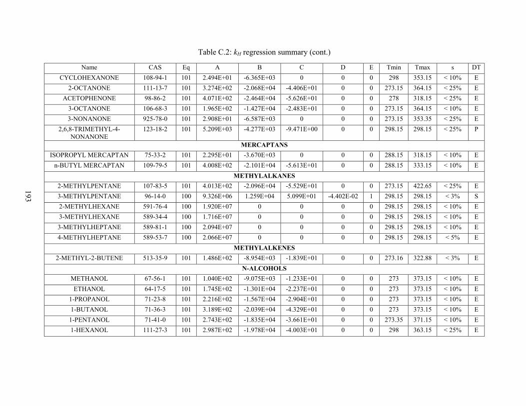
193

Table C.2: kH regression summary (cont.)

Name CAS Eq A B C D E Tmin Tmax s DT CYCLOHEXANONE 108-94-1 101 2.494E+01 -6.365E+03 0 0 0 298 353.15 < 10% E

2-OCTANONE 111-13-7 101 3.274E+02 -2.068E+04 -4.406E+01 0 0 273.15 364.15 < 25% E ACETOPHENONE 98-86-2 101 4.071E+02 -2.464E+04 -5.626E+01 0 0 278 318.15 < 25% E

3-OCTANONE 106-68-3 101 1.965E+02 -1.427E+04 -2.483E+01 0 0 273.15 364.15 < 10% E 3-NONANONE 925-78-0 101 2.908E+01 -6.587E+03 0 0 0 273.15 353.35 < 25% E

2,6,8-TRIMETHYL-4-NONANONE

123-18-2 101 5.209E+03 -4.277E+03 -9.471E+00 0 0 298.15 298.15 < 25% P

MERCAPTANS ISOPROPYL MERCAPTAN 75-33-2 101 2.295E+01 -3.670E+03 0 0 0 288.15 318.15 < 10% E

n-BUTYL MERCAPTAN 109-79-5 101 4.008E+02 -2.101E+04 -5.613E+01 0 0 288.15 333.15 < 10% E METHYLALKANES

2-METHYLPENTANE 107-83-5 101 4.013E+02 -2.096E+04 -5.529E+01 0 0 273.15 422.65 < 25% E 3-METHYLPENTANE 96-14-0 100 9.326E+06 1.259E+04 5.099E+01 -4.402E-02 1 298.15 298.15 < 3% S 2-METHYLHEXANE 591-76-4 100 1.920E+07 0 0 0 0 298.15 298.15 < 10% E 3-METHYLHEXANE 589-34-4 100 1.716E+07 0 0 0 0 298.15 298.15 < 10% E 3-METHYLHEPTANE 589-81-1 100 2.094E+07 0 0 0 0 298.15 298.15 < 10% E 4-METHYLHEPTANE 589-53-7 100 2.066E+07 0 0 0 0 298.15 298.15 < 5% E

METHYLALKENES 2-METHYL-2-BUTENE 513-35-9 101 1.486E+02 -8.954E+03 -1.839E+01 0 0 273.16 322.88 < 3% E

N-ALCOHOLS METHANOL 67-56-1 101 1.040E+02 -9.075E+03 -1.233E+01 0 0 273 373.15 < 10% E ETHANOL 64-17-5 101 1.745E+02 -1.301E+04 -2.237E+01 0 0 273 373.15 < 10% E

1-PROPANOL 71-23-8 101 2.216E+02 -1.567E+04 -2.904E+01 0 0 273 373.15 < 10% E 1-BUTANOL 71-36-3 101 3.189E+02 -2.039E+04 -4.329E+01 0 0 273 373.15 < 10% E

1-PENTANOL 71-41-0 101 2.743E+02 -1.835E+04 -3.661E+01 0 0 273.35 371.15 < 10% E 1-HEXANOL 111-27-3 101 2.987E+02 -1.978E+04 -4.003E+01 0 0 298 363.15 < 25% E

194

Table C.2: kH regression summary (cont.)

Name CAS Eq A B C D E Tmin Tmax s DT 1-HEPTANOL 111-70-6 101 3.399E+02 -2.193E+04 -4.593E+01 0 0 273 375 < 10% EP 1-OCTANOL 111-87-5 101 4.751E+02 -2.858E+04 -6.567E+01 0 0 288.15 363.45 < 10% EP 1-NONANOL 143-08-8 101 4.823E+02 -2.911E+04 -6.658E+01 0 0 288.15 363.15 < 25% E 1-DECANOL 112-30-1 101 5.385E+02 -3.155E+04 -7.495E+01 0 0 288.15 363.15 < 10% E

1-UNDECANOL 112-42-5 100 4.030E+02 0 0 0 0 298.15 298.15 < 50% P 1-DODECANOL 112-53-8 100 4.668E+02 0 0 0 0 298.15 298.15 < 50% P

N-ALIPHATIC PRIMARY AMINES ETHYLAMINE 75-04-7 100 6.618E+01 1.162E+04 2.974E+01 0 0 298.15 298.15 < 10% S

n-PROPYLAMINE 107-10-8 100 8.255E+01 1.063E+04 2.880E+01 0 0 298.15 298.15 < 10% S n-BUTYLAMINE 109-73-9 100 1.030E+02 1.277E+04 3.289E+01 0 0 298.15 298.15 < 10% S

n-PENTYLAMINE 110-58-7 100 1.284E+02 8.883E+03 2.125E+01 0 0 298.15 298.15 < 10% S n-HEXYLAMINE 111-26-2 100 1.602E+02 0 0 0 0 298.15 298.15 < 10% S n-HEPTYLAMINE 111-68-2 100 1.999E+02 0 0 0 0 298.15 298.15 < 25% S n-OCTYLAMINE 111-86-4 100 2.493E+02 0 0 0 0 298.15 298.15 < 25% S

N-ALKANES n-PENTANE 109-66-0 101 -1.239E+03 2.706E+04 2.257E+02 -4.087E-01 1 273.15 422.65 < 25% E n-HEXANE 110-54-3 101 4.056E+02 -2.109E+04 -5.595E+01 0 0 273.15 443.15 < 10% E n-HEPTANE 142-82-5 101 4.213E+02 -2.189E+04 -5.819E+01 0 0 273.15 443.75 < 25% E n-OCTANE 111-65-9 101 5.052E+02 -2.622E+04 -7.032E+01 0 0 273.15 456.15 < 25% E n-NONANE 111-84-2 101 7.275E+02 -3.721E+04 -1.028E+02 0 0 287.95 409.75 < 50% E n-DECANE 124-18-5 100 4.165E+07 0 0 0 0 298.15 298.15 < 50% S

N-ALKYLBENZENES BENZENE 71-43-2 101 6.091E+02 -2.377E+04 -9.619E+01 9.737E-02 1 273.15 527.15 < 3% E TOLUENE 108-88-3 101 6.605E+02 -2.545E+04 -1.049E+02 1.101E-01 1 261.7 473.55 < 5% E

ETHYLBENZENE 100-41-4 101 3.619E+02 -1.988E+04 -4.994E+01 0 0 273.15 373.15 < 5% E n-PROPYLBENZENE 103-65-1 101 2.463E+02 -1.450E+04 -3.276E+01 0 0 273.65 328.15 < 10% E

195

Table C.2: kH regression summary (cont.)

Name CAS Eq A B C D E Tmin Tmax s DT n-BUTYLBENZENE 104-51-8 101 4.132E+02 -2.226E+04 -5.744E+01 0 0 273.65 373.15 < 5% E n-HEPTYLBENZENE 1078-71-3 100 2.079E+05 -1.779E+04 -5.443E+01 0 0 298.15 298.15 < 10% P n-DECYLBENZENE 104-72-3 100 7.285E+05 0 0 0 0 298.15 298.15 < 10% S n-PENTYLBENZENE 538-68-1 101 4.005E+02 -2.240E+04 -5.510E+01 0 0 280.15 318.15 < 10% E n-HEXYLBENZENE 1077-16-3 101 3.675E+02 -2.136E+04 -4.985E+01 0 0 278.15 318.15 < 10% E n-OCTYLBENZENE 2189-60-8 100 3.005E+05 5.570E+03 0 0 0 298.15 298.15 < 10% P n-NONYLBENZENE 1081-77-2 100 3.866E+05 -4.112E+04 -2.080E+02 2.466E-01 1 298.15 298.15 < 25% P

NAPHTHALENES NAPHTHALENE 91-20-3 101 3.592E+02 -2.027E+04 -4.973E+01 0 0 275.05 346.55 < 3% E

1-METHYL-NAPHTHALENE

90-12-0 101 2.722E+01 -5.758E+03 0 0 0 277.25 304.85 < 10% E

2-METHYL-NAPHTHALENE

91-57-6 101 2.506E+01 -5.113E+03 0 0 0 277.25 304.15 < 25% E

1-ETHYL-NAPHTHALENE 1127-76-0 101 2.778E+01 -5.919E+03 0 0 0 281.55 304.85 < 10% E NITRILES

ACETONITRILE 75-05-8 101 -2.253E+00 -3.365E+03 3.205E+00 0 0 273 353.15 < 5% E PROPIONITRILE 107-12-0 101 9.456E+01 -7.820E+03 -1.110E+01 0 0 278.15 298.15 < 25% E

ACRYLONITRILE 107-13-1 101 1.926E+01 -3.863E+03 0 0 0 273.15 343.15 < 3% E METHACRYLONITRILE 126-98-7 101 2.729E+02 -1.537E+04 -3.756E+01 0 0 273.15 353.15 < 10% P

n-BUTYRONITRILE 109-74-0 101 1.333E+02 -1.001E+04 -1.650E+01 0 0 273.15 313.15 < 3% E VALERONITRILE 110-59-8 101 2.630E+01 -6.092E+03 0 0 0 273.15 303.15 < 25% E

ISOBUTYRONITRILE 78-82-0 101 2.382E+01 -5.246E+03 0 0 0 273.15 303.15 < 25% E BENZONITRILE 100-47-0 101 3.097E+02 -1.834E+04 -4.267E+01 0 0 273.15 363.15 < 25% E

VINYLACETONITRILE 109-75-1 101 2.209E+01 -4.916E+03 0 0 0 273.15 303.15 < 5% E PHENYLACETONITRILE 140-29-4 101 2.665E+01 -6.778E+03 0 0 0 273.15 303.15 < 100% E

NITROAMINES o-NITROANILINE 88-74-4 101 2.256E+01 -6.802E+03 0 0 0 298.15 313.25 < 50% E

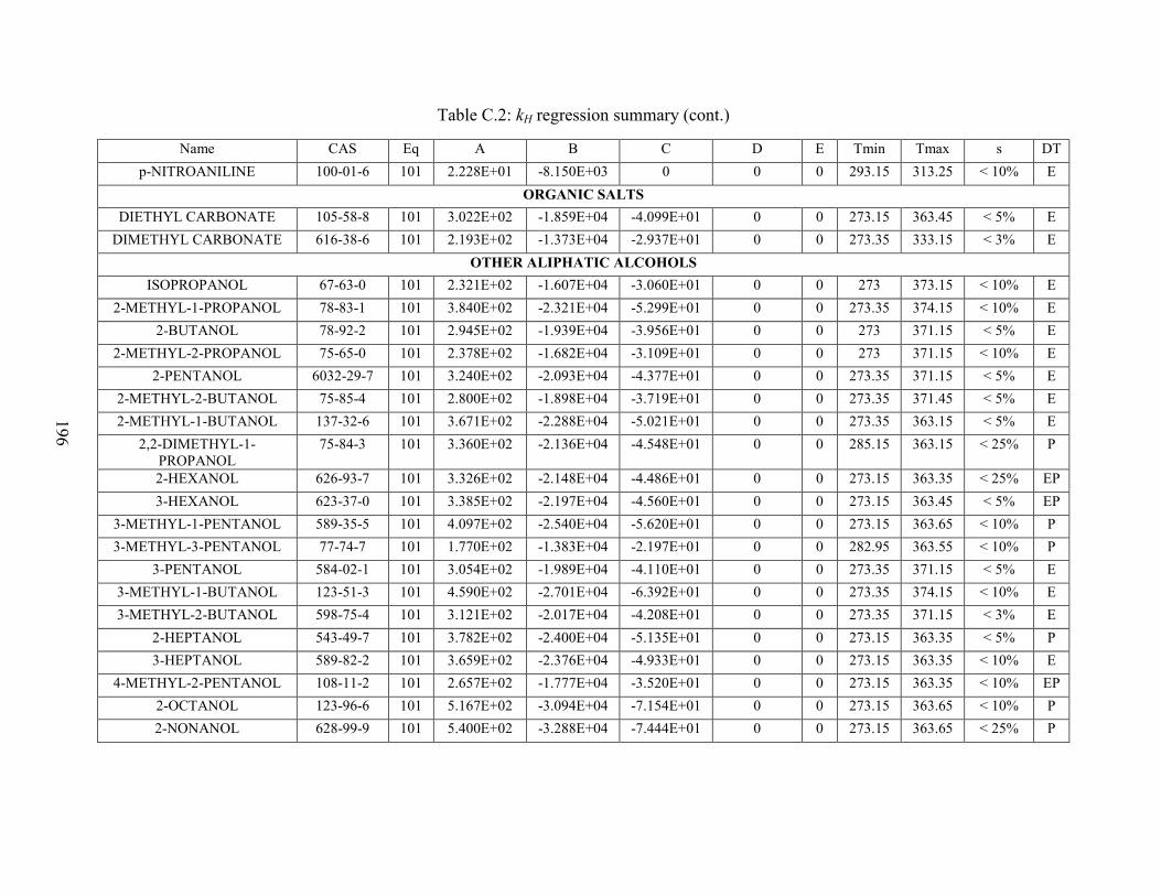
196

Table C.2: kH regression summary (cont.)

Name CAS Eq A B C D E Tmin Tmax s DT p-NITROANILINE 100-01-6 101 2.228E+01 -8.150E+03 0 0 0 293.15 313.25 < 10% E

ORGANIC SALTS DIETHYL CARBONATE 105-58-8 101 3.022E+02 -1.859E+04 -4.099E+01 0 0 273.15 363.45 < 5% E

DIMETHYL CARBONATE 616-38-6 101 2.193E+02 -1.373E+04 -2.937E+01 0 0 273.35 333.15 < 3% E OTHER ALIPHATIC ALCOHOLS

ISOPROPANOL 67-63-0 101 2.321E+02 -1.607E+04 -3.060E+01 0 0 273 373.15 < 10% E 2-METHYL-1-PROPANOL 78-83-1 101 3.840E+02 -2.321E+04 -5.299E+01 0 0 273.35 374.15 < 10% E

2-BUTANOL 78-92-2 101 2.945E+02 -1.939E+04 -3.956E+01 0 0 273 371.15 < 5% E 2-METHYL-2-PROPANOL 75-65-0 101 2.378E+02 -1.682E+04 -3.109E+01 0 0 273 371.15 < 10% E

2-PENTANOL 6032-29-7 101 3.240E+02 -2.093E+04 -4.377E+01 0 0 273.35 371.15 < 5% E 2-METHYL-2-BUTANOL 75-85-4 101 2.800E+02 -1.898E+04 -3.719E+01 0 0 273.35 371.45 < 5% E 2-METHYL-1-BUTANOL 137-32-6 101 3.671E+02 -2.288E+04 -5.021E+01 0 0 273.35 363.15 < 5% E

2,2-DIMETHYL-1-PROPANOL

75-84-3 101 3.360E+02 -2.136E+04 -4.548E+01 0 0 285.15 363.15 < 25% P

2-HEXANOL 626-93-7 101 3.326E+02 -2.148E+04 -4.486E+01 0 0 273.15 363.35 < 25% EP 3-HEXANOL 623-37-0 101 3.385E+02 -2.197E+04 -4.560E+01 0 0 273.15 363.45 < 5% EP

3-METHYL-1-PENTANOL 589-35-5 101 4.097E+02 -2.540E+04 -5.620E+01 0 0 273.15 363.65 < 10% P 3-METHYL-3-PENTANOL 77-74-7 101 1.770E+02 -1.383E+04 -2.197E+01 0 0 282.95 363.55 < 10% P

3-PENTANOL 584-02-1 101 3.054E+02 -1.989E+04 -4.110E+01 0 0 273.35 371.15 < 5% E 3-METHYL-1-BUTANOL 123-51-3 101 4.590E+02 -2.701E+04 -6.392E+01 0 0 273.35 374.15 < 10% E 3-METHYL-2-BUTANOL 598-75-4 101 3.121E+02 -2.017E+04 -4.208E+01 0 0 273.35 371.15 < 3% E

2-HEPTANOL 543-49-7 101 3.782E+02 -2.400E+04 -5.135E+01 0 0 273.15 363.35 < 5% P 3-HEPTANOL 589-82-2 101 3.659E+02 -2.376E+04 -4.933E+01 0 0 273.15 363.35 < 10% E

4-METHYL-2-PENTANOL 108-11-2 101 2.657E+02 -1.777E+04 -3.520E+01 0 0 273.15 363.35 < 10% EP 2-OCTANOL 123-96-6 101 5.167E+02 -3.094E+04 -7.154E+01 0 0 273.15 363.65 < 10% P 2-NONANOL 628-99-9 101 5.400E+02 -3.288E+04 -7.444E+01 0 0 273.15 363.65 < 25% P

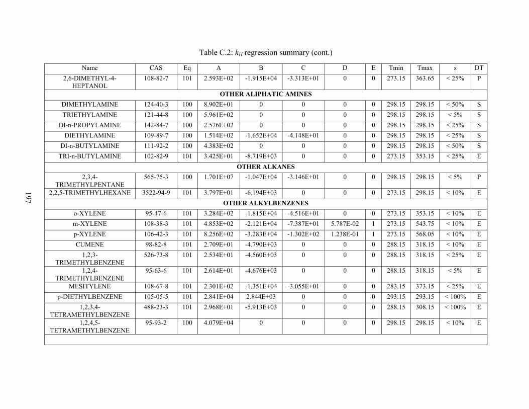
197

Table C.2: kH regression summary (cont.)

Name CAS Eq A B C D E Tmin Tmax s DT 2,6-DIMETHYL-4-

HEPTANOL 108-82-7 101 2.593E+02 -1.915E+04 -3.313E+01 0 0 273.15 363.65 < 25% P

OTHER ALIPHATIC AMINES DIMETHYLAMINE 124-40-3 100 8.902E+01 0 0 0 0 298.15 298.15 < 50% S TRIETHYLAMINE 121-44-8 100 5.961E+02 0 0 0 0 298.15 298.15 < 5% S

DI-n-PROPYLAMINE 142-84-7 100 2.576E+02 0 0 0 0 298.15 298.15 < 25% S DIETHYLAMINE 109-89-7 100 1.514E+02 -1.652E+04 -4.148E+01 0 0 298.15 298.15 < 25% S

DI-n-BUTYLAMINE 111-92-2 100 4.383E+02 0 0 0 0 298.15 298.15 < 50% S TRI-n-BUTYLAMINE 102-82-9 101 3.425E+01 -8.719E+03 0 0 0 273.15 353.15 < 25% E

OTHER ALKANES 2,3,4-

TRIMETHYLPENTANE 565-75-3 100 1.701E+07 -1.047E+04 -3.146E+01 0 0 298.15 298.15 < 5% P

2,2,5-TRIMETHYLHEXANE 3522-94-9 101 3.797E+01 -6.194E+03 0 0 0 273.15 298.15 < 10% E OTHER ALKYLBENZENES

o-XYLENE 95-47-6 101 3.284E+02 -1.815E+04 -4.516E+01 0 0 273.15 353.15 < 10% E m-XYLENE 108-38-3 101 4.853E+02 -2.121E+04 -7.387E+01 5.787E-02 1 273.15 543.75 < 10% E p-XYLENE 106-42-3 101 8.256E+02 -3.283E+04 -1.302E+02 1.238E-01 1 273.15 568.05 < 10% E CUMENE 98-82-8 101 2.709E+01 -4.790E+03 0 0 0 288.15 318.15 < 10% E

1,2,3-TRIMETHYLBENZENE

526-73-8 101 2.534E+01 -4.560E+03 0 0 0 288.15 318.15 < 25% E

1,2,4-TRIMETHYLBENZENE

95-63-6 101 2.614E+01 -4.676E+03 0 0 0 288.15 318.15 < 5% E

MESITYLENE 108-67-8 101 2.301E+02 -1.351E+04 -3.055E+01 0 0 283.15 373.15 < 25% E p-DIETHYLBENZENE 105-05-5 101 2.841E+04 2.844E+03 0 0 0 293.15 293.15 < 100% E

1,2,3,4-TETRAMETHYLBENZENE

488-23-3 101 2.968E+01 -5.913E+03 0 0 0 288.15 308.15 < 100% E

1,2,4,5-TETRAMETHYLBENZENE

95-93-2 100 4.079E+04 0 0 0 0 298.15 298.15 < 10% E

198

Table C.2: kH regression summary (cont.)

Name CAS Eq A B C D E Tmin Tmax s DT OTHER AMINES, IMINES

CYCLOHEXYLAMINE 108-91-8 101 2.024E+02 -1.528E+04 -2.596E+01 0 0 298.15 372.82 < 25% E TRIALLYLAMINE 102-70-5 101 4.010E+02 -2.393E+04 -5.502E+01 0 0 273.15 363.15 < 25% E

OTHER CONDENSED RINGS FLUORANTHENE 206-44-0 101 2.755E+01 -6.910E+03 0 0 0 281.25 333.15 < 10% E

FLUORENE 86-73-7 101 2.665E+01 -6.145E+03 0 0 0 279.75 333.15 < 10% E ANTHRACENE 120-12-7 101 3.683E+02 -2.185E+04 -5.088E+01 0 0 273.45 347.85 < 5% E

PHENANTHRENE 85-01-8 101 4.223E+02 -2.462E+04 -5.873E+01 0 0 277.15 346.55 < 5% E CHRYSENE 218-01-9 101 4.104E+01 -1.184E+04 0 0 0 279.65 302.15 < 25% E

PYRENE 129-00-0 101 3.078E+02 -1.937E+04 -4.193E+01 0 0 277.85 347.85 < 5% E ACENAPHTHENE 83-32-9 101 2.469E+01 -5.381E+03 0 0 0 277.25 347.85 < 25% E

ACENAPHTHALENE 208-96-8 101 2.748E+01 -6.263E+03 0 0 0 277.25 304.15 < 25% E BENZO[a]PYRENE 50-32-8 101 3.108E+01 -8.515E+03 0 0 0 281.15 308.15 < 10% E

BENZO[b]FLUORANTHENE 205-99-2 101 1.949E+01 -5.422E+03 0 0 0 283.15 328.15 < 10% E OTHER ETHERS/DIETHERS

METHYLAL 109-87-5 101 2.270E+01 -4.738E+03 0 0 0 273.35 333.15 < 25% E 1,2-DIMETHOXYETHANE 110-71-4 101 2.511E+02 -1.722E+04 -3.328E+01 0 0 273.35 372.5 < 3% E

DIETHYLENE GLYCOL DI-n-BUTYL ETHER

112-73-2 101 4.602E+01 -1.280E+04 0 0 0 273.15 293.15 < 100% P

ANISOLE 100-66-3 101 2.158E+01 -4.179E+03 0 0 0 275.15 363.85 < 5% E DIPHENYL ETHER 101-84-8 100 2.903E+03 0 0 0 0 298.15 298.15 < 50% S

OTHER INORGANICS HYDROGEN PEROXIDE 7722-84-1 101 2.142E+01 -7.235E+03 0 0 0 278.15 297.15 < 25% E

OTHER MONOAROMATICS STYRENE 100-42-5 101 2.190E+01 -3.653E+03 0 0 0 293.32 313.02 < 5% E

199

Table C.2: kH regression summary (cont.)

Name CAS Eq A B C D E Tmin Tmax s DT OTHER POLYFUNCTIONAL C, H, O

2-BUTOXYETHANOL 111-76-2 101 2.922E+01 -8.275E+03 0 0 0 293.15 303.15 < 25% E VANILLIN 121-33-5 101 -3.909E+02 1.144E+04 6.127E+01 0 0 293.15 318.15 < 5% E

OTHER POLYFUNCTIONAL ORGANICS MALATHION 121-75-5 101 2.879E+01 -8.274E+03 0 0 0 283.15 303.15 < 25% E

OTHER SATURATED ALIPHATIC ESTERS ETHYL ISOVALERATE 108-64-5 101 2.443E+02 -1.600E+04 -3.201E+01 0 0 273.15 363.65 < 10% E DIETHYL MALONATE 105-53-3 101 2.731E+02 -1.846E+04 -3.660E+01 0 0 273.15 363.75 < 10% P DIETHYL SUCCINATE 123-25-1 ETHYL TRIMETHYL

ACETATE 3938-95-2 101 2.619E+02 -1.693E+04 -3.441E+01 0 0 273.15 363.55 < 25% E

PEROXIDES METHYL

HYDROPEROXIDE 3031-73-0 101 2.049E+01 -5.244E+03 0 0 0 277.15 297.15 < 3% E

ETHYL HYDROPEROXIDE 3031-74-1 101 2.288E+01 -5.985E+03 0 0 0 278.15 297.15 < 10% E POLYFUNCTIONAL AMIDES/AMINES

N,N-DIMETHYLFORMAMIDE

68-12-2 101 2.051E+02 -1.570E+04 -2.692E+01 0 0 289.4 372 < 25% E

N-METHYLFORMAMIDE 123-39-7 101 2.081E+01 -7.161E+03 0 0 0 333.15 372.65 < 5% E N,N-

DIMETHYLACETAMIDE 127-19-5 101 2.480E+01 -8.014E+03 0 0 0 343.15 372.28 < 10% E

POLYFUNCTIONAL C, H, N, HALIDE, (O) o-CHLOROANILINE 95-51-2 101 1.336E+03 -5.042E+04 -2.173E+02 2.501E-01 1 298.15 431.15 < 25% P

p-CHLORONITROBENZENE

100-00-5 101 2.414E+01 -5.868E+03 0 0 0 283.15 313.15 < 10% E

POLYFUNCTIONAL C, H, O, HALIDE DI(2-

CHLOROETHYL)ETHER 111-44-4 101 2.107E+02 -1.440E+04 -2.767E+01 0 0 273.15 364.85 < 5% E

ETHYLCHLOROACETATE 105-39-5 101 2.546E+02 -1.630E+04 -3.415E+01 0 0 273.15 333.25 < 10% E

200

Table C.2: kH regression summary (cont.)

Name CAS Eq A B C D E Tmin Tmax s DT METHYL

CHLOROACETATE 96-34-4 101 1.755E+02 -1.239E+04 -2.268E+01 0 0 273.15 323.35 < 5% E

POLYFUNCTIONAL C, H, O, N N-METHYL-2-

PYRROLIDONE 872-50-4 101 4.600E+02 -3.011E+04 -6.372E+01 0 0 298.8 372.85 < 5% E

POLYFUNCTIONAL C, H, O, S DIMETHYL SULFOXIDE 67-68-5 101 2.115E+01 -7.789E+03 0 0 0 298.8 337.9 < 25% E

POLYFUNCTIONAL ESTERS METHYL SALICYLATE 119-36-8 101 4.635E+02 -2.852E+04 -6.394E+01 0 0 273.15 363.65 < 25% E

2-ETHOXYETHYL ACETATE

111-15-9 100 1.850E+01 0 0 0 0 303.15 303.15 < 10% E

ETHYL ACETOACETATE 141-97-9 101 2.610E+01 -7.239E+03 0 0 0 273.15 303.15 < 25% EP ETHYLENE GLYCOL MONOBUTYL ETHER

ACETATE

112-07-2 100 3.062E+01 0 0 0 0 298.15 298.15 < 25% E

PROPIONATES AND BUTYRATES METHYL PROPIONATE 554-12-1 101 2.605E+01 -5.719E+03 0 0 0 273.15 310.2 < 5% E ETHYL PROPIONATE 105-37-3 101 2.963E+02 -1.786E+04 -4.021E+01 0 0 273.15 353.45 < 25% E

n-PROPYL PROPIONATE 106-36-5 101 2.299E+02 -1.536E+04 -2.996E+01 0 0 273.15 363.65 < 10% E n-BUTYL PROPIONATE 590-01-2 101 2.785E+02 -1.795E+04 -3.694E+01 0 0 273.15 363.55 < 10% E n-PROPYL n-BUTYRATE 105-66-8 101 2.587E+02 -1.660E+04 -3.422E+01 0 0 273.15 363.65 < 25% E METHYL n-BUTYRATE 623-42-7 101 1.665E+02 -1.196E+04 -2.091E+01 0 0 273.15 363.65 < 25% E ETHYL n-BUTYRATE 105-54-4 101 1.949E+02 -1.355E+04 -2.488E+01 0 0 273.15 363.65 < 25% E

ISOBUTYL ISOBUTYRATE 97-85-8 101 2.887E+02 -1.832E+04 -3.832E+01 0 0 273.15 363.45 < 25% E n-BUTYL n-BUTYRATE 109-21-7 101 3.706E+02 -2.260E+04 -5.032E+01 0 0 273.15 363.45 < 10% E

METHYL ISOBUTYRATE 547-63-7 101 2.024E+02 -1.347E+04 -2.625E+01 0 0 273.15 353.45 < 10% E ETHYL ISOBUTYRATE 97-62-1 101 1.871E+02 -1.308E+04 -2.370E+01 0 0 273.15 363.75 < 10% P

n-PENTYL n-BUTYRATE 540-18-1 101 2.955E+01 -6.393E+03 0 0 0 273.15 363.65 < 25% E

201

Table C.2: kH regression summary (cont.)

Name CAS Eq A B C D E Tmin Tmax s DT ISOPENTYL BUTYRATE 106-27-4 101 3.076E+02 -1.973E+04 -4.087E+01 0 0 282.55 363.85 < 100% E

SULFIDES/THIOPHENES DIMETHYL SULFIDE 75-18-3 101 2.083E+02 -1.184E+04 -2.797E+01 0 0 272.35 353.45 < 10% E

DIMETHYL DISULFIDE 624-92-0 101 2.120E+01 -3.695E+03 0 0 0 273.2 343.15 < 10% E 2-METHYLTHIOPHENE 554-14-3 101 2.390E+01 -4.287E+03 0 0 0 298.15 343.15 < 10% E DIISOPROPYL SULFIDE 625-80-9 101 2.628E+01 -4.889E+03 0 0 0 298.15 343.15 < 10% E

UNSATURATED ALIPHATIC ESTERS ETHYL ACRYLATE 140-88-5 101 2.199E+01 -4.393E+03 0 0 0 298.6 360.2 < 10% P

METHYL METHACRYLATE

80-62-6 101 2.853E+02 -1.690E+04 -3.880E+01 0 0 273.35 333.15 < 3% E

Table C.3: γi∞ regression summary (cont.)

Name CAS Eq A B C D E Tmin Tmax s DT 1-ALKENES

1-PENTENE 109-67-1 100 2.2033E+04 0 0 0 0 298.15 298.15 < 25% S 1-HEXENE 592-41-6 100 9.1053E+04 4.5755E+03 5.6855E+00 0 0 298.15 298.15 < 25% S 1-HEPTENE 592-76-7 100 3.7625E+05 0 0 0 0 298.15 298.15 < 10% S 1-OCTENE 111-66-0 100 1.5549E+06 0 0 0 0 298.15 298.15 < 10% S 1-NONENE 124-11-8 100 6.4250E+06 0 0 0 0 298.15 298.15 < 25% S 1-DECENE 872-05-9 100 2.6552E+07 0 0 0 0 298.15 298.15 < 25% P 1-UNDECENE 872-05-9 100 1.0973E+08 0 0 0 0 298.15 298.15 < 25% P 1-DODECENE 872-05-9 100 4.5341E+08 0 0 0 0 298.15 298.15 < 25% P 1-TRIDECENE 592-41-6 100 1.8737E+09 0 0 0 0 298.15 298.15 < 50% P 1-TETRADECENE 872-05-9 100 7.7426E+09 0 0 0 0 298.15 298.15 < 50% P 1-PENTADECENE 13360-61-7 100 3.1997E+10 0 0 0 0 298.15 298.15 < 50% S

202

Table C.3: γi∞ regression summary (cont.)

Name CAS Eq A B C D E Tmin Tmax s DT 2,3,4-ALKENES

cis-2-PENTENE 627-20-3 100 1.9178E+04 0 0 0 0 298.15 298.15 < 5% E trans-2-PENTENE 646-04-8 100 1.9178E+04 0 0 0 0 298.15 298.15 < 5% E cis-2-HEPTENE 6443-92-1 100 3.6334E+05 0 0 0 0 298.15 298.15 < 10% E trans-2-HEPTENE 14686-13-6 100 3.6334E+05 0 0 0 0 298.15 298.15 < 10% E

ACETATES METHYL ACETATE 79-20-9 101 4.0958E+02 -1.9719E+04 -5.9724E+01 0 0 293.15 343.25 < 10% E ETHYL ACETATE 141-78-6 101 1.8730E+02 -9.2371E+03 -2.6696E+01 0 0 288.15 353.15 < 10% E n-PROPYL ACETATE 109-60-4 101 2.2269E+02 -1.0697E+04 -3.1801E+01 0 0 298 343.25 < 10% E n-BUTYL ACETATE 123-86-4 101 1.7311E+02 -8.2435E+03 -2.4321E+01 0 0 273.15 363.65 < 10% E ISOBUTYL ACETATE 110-19-0 101 2.9865E+01 -1.9167E+03 -2.9174E+00 0 0 273.15 323.15 < 25% E ISOPENTYL ACETATE 123-92-2 101 2.3843E+02 -1.1153E+04 -3.3853E+01 0 0 273.15 363.85 < 10% E ISOPROPYL ACETATE 108-21-4 101 -1.0523E+02 3.4976E+03 1.7345E+01 0 0 273.15 310.2 < 25% E sec-BUTYL ACETATE 105-46-4 101 1.8364E+02 -8.8655E+03 -2.5835E+01 0 0 273.15 363.65 < 10% E VINYL ACETATE 108-05-4 101 1.3344E+02 -6.0176E+03 -1.8964E+01 0 0 273.35 333.15 < 3% E n-PENTYL ACETATE 628-63-7 101 3.3660E+02 -1.5786E+04 -4.8331E+01 0 0 273.15 364.5 < 25% E n-HEXYL ACETATE 142-92-7 101 3.7674E+02 -1.7146E+04 -5.4324E+01 0 0 273.15 363.35 < 25% E n-HEPTYL ACETATE 112-06-1 100 6.5861E+04 -1.8462E+04 -3.6599E+01 0 0 298.15 298.15 < 25% P n-OCTYL ACETATE 112-14-1 100 2.6455E+05 -2.1364E+04 -4.5483E+01 0 0 298.15 298.15 < 25% P tert-BUTYL ACETATE 540-88-5 101 1.6617E+02 -8.2029E+03 -2.3147E+01 0 0 273.15 353.65 < 10% E CYCLOHEXYL ACETATE 622-45-7 101 2.0341E+02 -9.4699E+03 -2.8728E+01 0 0 273.15 363.45 < 10% E PHENYL ACETATE 122-79-2 101 1.6704E+02 -7.1054E+03 -2.3876E+01 0 0 273.15 363.95 < 10% E

ALDEHYDES PROPANAL 123-38-6 101 2.3549E+02 -1.1978E+04 -3.3870E+01 0 0 278.15 318.15 < 5% E BUTANAL 123-72-8 101 1.0100E+01 -1.9064E+03 0 0 0 278.15 318.15 < 10% E 2-METHYLPROPANAL 78-84-2 100 5.1912E+01 -6.5156E+03 -2.1156E+01 -8.2308E-06 2 298.15 298.15 < 5% S

203

Table C.3: γi∞ regression summary (cont.)

Name CAS Eq A B C D E Tmin Tmax s DT PENTANAL 110-62-3 101 1.1248E+01 -1.7998E+03 0 0 0 278.15 318.15 < 10% E HEPTANAL 111-71-7 101 1.4484E+01 -1.9125E+03 0 0 0 283.15 318.15 < 25% E HEXANAL 66-25-1 101 1.0459E+01 -1.1086E+03 0 0 0 283.15 318.15 < 25% E OCTANAL 124-13-0 101 1.3249E+01 -1.0346E+03 0 0 0 283.15 318.15 < 10% E NONANAL 124-19-6 101 8.9172E+00 8.7039E+02 0 0 0 283.15 318.15 < 25% E 2-ETHYLHEXANAL 123-05-7 101 8.2330E+00 4.5752E+02 0 0 0 273.15 363.15 < 25% E 2-ETHYL-2-HEXENAL 645-62-5 101 8.3085E+00 1.0122E+02 0 0 0 273.15 363.15 < 50% E DECANAL 112-31-2 101 1.6820E+01 -1.0090E+03 0 0 0 298.15 318.15 < 50% E 2-METHYL-BUTYRALDEHYDE

96-17-3 101 9.8196E+00 -1.2187E+03 0 0 0 273.15 363.15 < 25% P

ACROLEIN 107-02-8 101 7.9257E+00 -1.4558E+03 0 0 0 273 298 < 100% E trans-CROTONALDEHYDE 123-73-9 101 1.2597E+02 -5.9638E+03 -1.8057E+01 0 0 273.15 363.15 < 25% EP METHACROLEIN 78-85-3 101 6.5218E+00 -7.1561E+02 0 0 0 273.15 333.15 < 10% E p-TOLUALDEHYDE 104-87-0 101 9.6622E+00 -5.4954E+02 0 0 0 278 298 < 25% E BENZALDEHYDE 100-52-7 101 5.1540E+02 -2.1901E+04 -7.6382E+01 0 0 273.08 323.15 < 10% E m-TOLUALDEHYDE 620-23-5 101 9.4640E+00 -3.8418E+02 0 0 0 278 298 < 25% E

ALIPHATIC ETHERS DIETHYL ETHER 60-29-7 101 2.3981E+02 -1.2537E+04 -3.3940E+01 0 0 273.35 333.25 < 5% E DIISOPROPYL ETHER 108-20-3 101 -4.6536E+01 7.2880E+01 9.2540E+00 0 0 273.15 334.15 < 10% E DI-n-BUTYL ETHER 142-96-1 101 1.4973E+01 -1.3729E+03 0 0 0 273.15 363.65 < 25% E METHYL tert-BUTYL ETHER

1634-04-4 101 5.7408E+01 -4.2388E+03 -6.7324E+00 0 0 273.15 343.15 < 10% E

METHYL ISOBUTYL ETHER

625-44-5 101 1.5503E+01 -2.8030E+03 0 0 0 273.15 298.15 < 5% E

DI-n-HEXYL ETHER 112-58-3 100 1.4510E+07 -1.8280E+04 -5.4709E+01 0 0 298.15 298.15 < 25% P METHYL n-BUTYL ETHER 628-28-4 101 7.0311E+02 -3.2841E+04 -1.0296E+02 0 0 273.15 298.15 < 25% E DI-n-PENTYL ETHER 693-65-2 100 4.5100E+05 -7.0534E+03 -2.2745E+01 0 0 298.15 298.15 < 25% P

204

Table C.3: γi∞ regression summary (cont.)

Name CAS Eq A B C D E Tmin Tmax s DT METHYL tert-PENTYL ETHER

994-05-8 101 1.7808E+02 -9.7068E+03 -2.4430E+01 0 0 273.15 352.35 < 10% E

tert-BUTYL ETHYL ETHER 637-92-3 101 1.5616E+01 -2.8259E+03 0 0 0 278.15 318.15 < 25% E ETHYL tert-PENTYL ETHER 919-94-8 101 1.7640E+01 -2.9893E+03 0 0 0 288.15 318.15 < 25% E DI-n-PROPYL ETHER 111-43-3 101 4.0286E+02 -1.9387E+04 -5.7942E+01 0 0 273.15 333.25 < 5% E n-BUTYL ETHYL ETHER 628-81-9 101 2.0852E+02 -1.0117E+04 -2.9431E+01 0 0 273.15 363.85 < 25% E

ALKYLCYCLOHEXANES METHYLCYCLOHEXANE 108-87-2 101 3.6535E+02 -1.5923E+04 -5.2511E+01 0 0 293.15 443.95 < 25% E ETHYLCYCLOHEXANE 1678-91-7 101 1.7556E+03 -5.4303E+04 -2.9260E+02 3.6218E-01 1 273.15 443.95 < 10% E cis-1,2-DIMETHYL-CYCLOHEXANE

2207-01-4 101 3.3288E+02 -1.3995E+04 -4.7754E+01 0 0 273.15 313.15 < 25% E

trans-1,2-DIMETHYL-CYCLOHEXANE

6876-23-9 101 1.4668E+03 -4.6285E+04 -2.4271E+02 2.8645E-01 1 273.15 443.25 < 5% E

ALKYLCYCLOPENTANES METHYL-CYCLOPENTANE 96-37-7 100 1.0935E+05 -7.8306E+03 -2.7270E+01 -6.3208E-06 2 298.15 298.15 < 3% S

ALKYNES 1-PENTYNE 627-19-0 100 2.4720E+03 0 0 0 0 298.15 298.15 < 25% S 1-HEXYNE 693-02-7 100 1.1810E+04 0 0 0 0 298.15 298.15 < 25% S 1-OCTYNE 629-05-0 100 2.5340E+05 0 0 0 0 298.15 298.15 < 25% S 1-NONYNE 3452-09-3 100 1.3100E+06 0 0 0 0 298.15 298.15 < 25% S 1-HEPTYNE 628-71-7 100 5.4810E+04 0 0 0 0 298.15 298.15 < 25% S

AROMATIC ALCOHOLS 2,3-XYLENOL 526-75-0 101 3.2073E+00 9.3895E+02 0 0 0 349.05 371.65 < 25% S 2,4-XYLENOL 105-67-9 101 1.6630E+00 1.5325E+03 0 0 0 349.05 371.65 < 25% E 2,5-XYLENOL 95-87-4 101 3.4136E+02 -1.5740E+04 -4.9567E+01 0 0 278 371.65 < 10% E 2,6-XYLENOL 576-26-1 101 1.2864E+02 -4.9837E+03 -1.8451E+01 0 0 278 371.65 < 10% E 3,4-XYLENOL 95-65-8 101 3.2111E+00 8.9290E+02 0 0 0 293.15 371.65 < 25% E

205

Table C.3: γi∞ regression summary (cont.)

Name CAS Eq A B C D E Tmin Tmax s DT 3,5-XYLENOL 108-68-9 101 1.1755E+02 -4.5606E+03 -1.6823E+01 0 0 293.15 371.65 < 25% E PHENOL 108-95-2 101 4.5472E+02 -2.1677E+04 -6.6388E+01 0 0 278 373.15 < 25% E o-CRESOL 95-48-7 101 2.1997E+02 -9.7201E+03 -3.1956E+01 0 0 293.15 371.65 < 5% E m-CRESOL 108-39-4 101 -1.5582E+01 2.1554E+03 2.4416E+00 0 0 298.15 371.65 < 25% E p-CRESOL 106-44-5 101 1.5458E+02 -6.2545E+03 -2.2485E+01 0 0 298 371.65 < 3% E 2-PHENYLETHANOL 60-12-8 101 1.7589E+02 -7.4876E+03 -2.5479E+01 0 0 283.15 373.15 < 10% P

AROMATIC AMINES o-TOLUIDINE 95-53-4 101 5.6946E+00 3.2271E+01 0 0 0 298.15 323.15 < 25% E m-TOLUIDINE 108-44-1 101 5.6591E+00 8.1355E+01 0 0 0 298.15 323.15 < 25% E p-TOLUIDINE 106-49-0 101 6.3431E-01 1.6356E+03 0 0 0 293.15 313.15 < 5% P N,N-DIETHYLANILINE 91-66-7 101 9.2931E+00 4.2183E+02 0 0 0 273.15 333.15 < 25% E PYRIDINE 110-86-1 101 3.2354E+00 -4.9087E+01 0 0 0 298 374.15 < 25% E ANILINE 62-53-3 101 1.8127E+02 -8.1850E+03 -2.6142E+01 0 0 298 374.15 < 10% E 2-METHYLPYRIDINE 109-06-8 101 7.8877E+00 -1.2722E+03 0 0 0 298 313.15 < 5% E o-ETHYLANILINE 578-54-1 101 1.6012E+02 -7.0534E+03 -2.2745E+01 0 0 283.15 363.15 < 10% P 2,6-DIMETHYLPYRIDINE 108-48-5 101 1.1003E+01 -1.9828E+03 0 0 0 298 313.15 < 25% E 3-METHYLPYRIDINE 108-99-6 101 7.5009E+00 -1.0441E+03 0 0 0 298 313.15 < 25% E 4-METHYLPYRIDINE 108-89-4 101 7.6057E+00 -1.1383E+03 0 0 0 298 313.15 < 5% E 2,4-DIMETHYLANILINE 95-68-1 101 2.6650E+02 -1.2031E+04 -3.8444E+01 0 0 273.15 363.15 < 25% P N-ETHYLANILINE 103-69-5 101 1.8651E+02 -8.4052E+03 -2.6420E+01 0 0 273.15 363.15 < 10% E

AROMATIC CHLORIDES BENZYL CHLORIDE 100-44-7 101 4.7978E+00 1.4249E+03 0 0 0 277.65 303.15 < 25% E MONOCHLOROBENZENE 108-90-7 101 3.0084E+02 -1.1883E+04 -4.4139E+01 0 0 274.15 353.16 < 10% E o-DICHLOROBENZENE 95-50-1 101 7.4286E+02 -3.1963E+04 -1.0964E+02 0 0 278.15 318.15 < 10% E m-DICHLOROBENZENE 541-73-1 101 7.3203E+00 1.1112E+03 0 0 0 278.15 318.15 < 10% E p-DICHLOROBENZENE 106-46-7 101 5.2227E+02 -2.3008E+04 -7.6204E+01 0 0 278.15 346.55 < 10% E

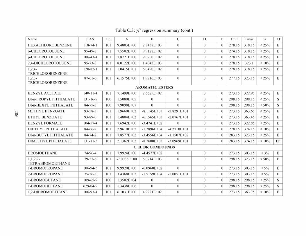
206

Table C.3: γi∞ regression summary (cont.)

Name CAS Eq A B C D E Tmin Tmax s DT HEXACHLOROBENZENE 118-74-1 101 9.4803E+00 2.8438E+03 0 0 0 278.15 318.15 < 25% E o-CHLOROTOLUENE 95-49-8 101 7.5502E+00 9.9128E+02 0 0 0 274.15 318.15 < 25% E p-CHLOROTOLUENE 106-43-4 101 7.8721E+00 9.0900E+02 0 0 0 278.15 318.15 < 25% E 2,4-DICHLOROTOLUENE 95-73-8 101 8.0122E+00 1.4043E+03 0 0 0 278.15 323.1 < 10% E 1,2,4-TRICHLOROBENZENE

120-82-1 101 1.0415E+01 6.0490E+02 0 0 0 278.15 318.15 < 25% E

1,2,3-TRICHLOROBENZENE

87-61-6 101 6.1575E+00 1.9216E+03 0 0 0 277.15 323.15 < 25% E

AROMATIC ESTERS BENZYL ACETATE 140-11-4 101 7.1499E+00 2.6685E+02 0 0 0 273.15 322.95 < 25% E DI-n-PROPYL PHTHALATE 131-16-8 100 1.5080E+05 0 0 0 0 298.15 298.15 < 25% S DI-n-HEXYL PHTHALATE 84-75-3 100 7.9098E+07 0 0 0 0 298.15 298.15 < 50% S METHYL BENZOATE 93-58-3 101 1.9660E+02 -8.1145E+03 -2.8291E+01 0 0 273.15 363.65 < 25% E ETHYL BENZOATE 93-89-0 101 1.4804E+02 -6.1565E+03 -2.0767E+01 0 0 273.15 363.45 < 25% E BENZYL FORMATE 104-57-4 101 7.6942E+00 -3.4741E+02 0 0 0 273.15 322.85 < 25% E DIETHYL PHTHALATE 84-66-2 101 2.9610E+02 -1.2896E+04 -4.2710E+01 0 0 278.15 374.15 < 10% E DI-n-BUTYL PHTHALATE 84-74-2 101 7.8577E+02 -3.4556E+04 -1.1507E+02 0 0 283.15 323.15 < 25% E DIMETHYL PHTHALATE 131-11-3 101 2.1362E+02 -8.7600E+03 -3.0969E+01 0 0 283.15 374.15 < 10% EP

C, H, BR COMPOUNDS BROMOETHANE 74-96-4 101 7.9924E+00 -4.4577E+02 0 0 0 273.15 303.15 < 3% E 1,1,2,2-TETRABROMOETHANE

79-27-6 101 -7.0038E+00 6.0714E+03 0 0 0 298.15 323.15 < 50% E

1-BROMOPROPANE 106-94-5 101 9.9920E+00 -6.0960E+02 0 0 0 273.15 303.15 < 5% E 2-BROMOPROPANE 75-26-3 101 3.4368E+02 -1.5159E+04 -5.0051E+01 0 0 273.15 303.15 < 5% E 1-BROMOBUTANE 109-65-9 100 1.3502E+04 0 0 0 0 298.15 298.15 < 25% S 1-BROMOHEPTANE 629-04-9 100 1.3438E+06 0 0 0 0 298.15 298.15 < 25% S 1,2-DIBROMOETHANE 106-93-4 101 6.1031E+00 4.9221E+02 0 0 0 273.15 363.75 < 10% E

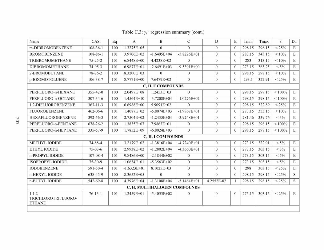
207

Table C.3: γi∞ regression summary (cont.)

Name CAS Eq A B C D E Tmin Tmax s DT m-DIBROMOBENZENE 108-36-1 100 1.3275E+05 0 0 0 0 298.15 298.15 < 25% E BROMOBENZENE 108-86-1 101 3.9706E+02 -1.6495E+04 -5.8226E+01 0 0 283.15 343.15 < 10% E TRIBROMOMETHANE 75-25-2 101 6.8448E+00 4.4238E+02 0 0 0 283 313.15 < 10% E DIBROMOMETHANE 74-95-3 101 6.9877E+01 -2.6491E+03 -9.5301E+00 0 0 273.15 363.25 < 5% E 2-BROMOBUTANE 78-76-2 100 8.3200E+03 0 0 0 0 298.15 298.15 < 10% E p-BROMOTOLUENE 106-38-7 101 8.7771E+00 7.6479E+02 0 0 0 293.1 322.91 < 25% E

C, H, F COMPOUNDS PERFLUORO-n-HEXANE 355-42-0 100 2.0497E+08 1.2453E+03 0 0 0 298.15 298.15 < 100% E PERFLUORO-n-OCTANE 307-34-6 100 1.4564E+10 -3.7208E+04 -1.0276E+02 0 0 298.15 298.15 < 100% E 1,2-DIFLUOROBENZENE 367-11-3 101 6.6988E+00 5.9091E+02 0 0 0 298.15 322.89 < 25% E FLUOROBENZENE 462-06-6 101 1.4087E+02 -5.8074E+03 -1.9867E+01 0 0 273.15 353.15 < 10% E HEXAFLUOROBENZENE 392-56-3 101 2.7504E+02 -1.2435E+04 -3.9248E+01 0 0 281.46 339.76 < 3% E PERFLUORO-n-PENTANE 678-26-2 100 1.3835E+07 7.9863E+01 0 0 0 298.15 298.15 < 100% E PERFLUORO-n-HEPTANE 335-57-9 100 1.7852E+09 -6.8024E+03 0 0 0 298.15 298.15 < 100% E

C, H, I COMPOUNDS METHYL IODIDE 74-88-4 101 3.2179E+02 -1.3816E+04 -4.7240E+01 0 0 273.15 322.91 < 5% E ETHYL IODIDE 75-03-6 101 2.9938E+02 -1.2802E+04 -4.3660E+01 0 0 273.15 303.15 < 3% E n-PROPYL IODIDE 107-08-4 101 9.8486E+00 -2.1844E+02 0 0 0 273.15 303.15 < 5% E ISOPROPYL IODIDE 75-30-9 101 1.0634E+01 -5.3563E+02 0 0 0 273.15 303.15 < 5% E IODOBENZENE 591-50-4 101 -1.6323E+01 8.1025E+03 0 0 0 298 303.15 < 25% E n-HEXYL IODIDE 638-45-9 100 8.3652E+05 0 0 0 0 298.15 298.15 < 25% S n-BUTYL IODIDE 542-69-8 100 4.3976E+04 -1.3108E+04 -5.1464E+01 4.2552E-02 1 298.15 298.15 < 25% S

C, H, MULTIHALOGEN COMPOUNDS 1,1,2-TRICHLOROTRIFLUORO-ETHANE

76-13-1 101 1.2459E+01 -5.4053E+02 0 0 0 275.15 303.15 < 25% E

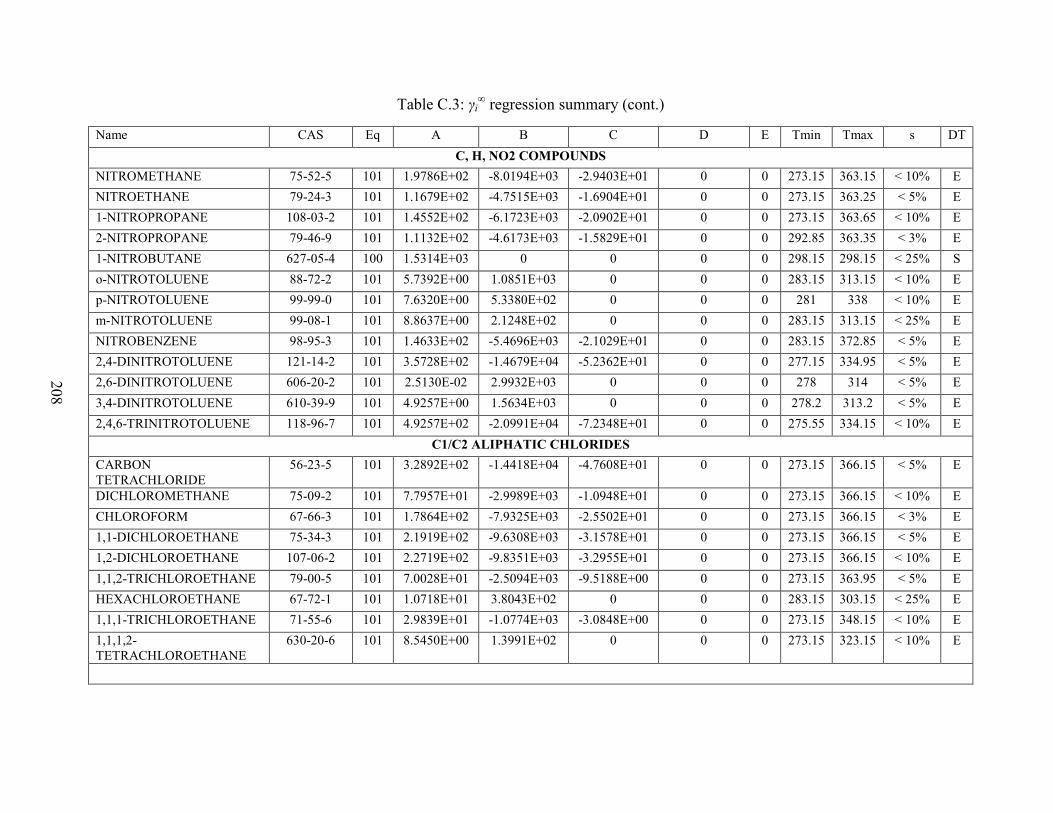
208

Table C.3: γi∞ regression summary (cont.)

Name CAS Eq A B C D E Tmin Tmax s DT C, H, NO2 COMPOUNDS

NITROMETHANE 75-52-5 101 1.9786E+02 -8.0194E+03 -2.9403E+01 0 0 273.15 363.15 < 10% E NITROETHANE 79-24-3 101 1.1679E+02 -4.7515E+03 -1.6904E+01 0 0 273.15 363.25 < 5% E 1-NITROPROPANE 108-03-2 101 1.4552E+02 -6.1723E+03 -2.0902E+01 0 0 273.15 363.65 < 10% E 2-NITROPROPANE 79-46-9 101 1.1132E+02 -4.6173E+03 -1.5829E+01 0 0 292.85 363.35 < 3% E 1-NITROBUTANE 627-05-4 100 1.5314E+03 0 0 0 0 298.15 298.15 < 25% S o-NITROTOLUENE 88-72-2 101 5.7392E+00 1.0851E+03 0 0 0 283.15 313.15 < 10% E p-NITROTOLUENE 99-99-0 101 7.6320E+00 5.3380E+02 0 0 0 281 338 < 10% E m-NITROTOLUENE 99-08-1 101 8.8637E+00 2.1248E+02 0 0 0 283.15 313.15 < 25% E NITROBENZENE 98-95-3 101 1.4633E+02 -5.4696E+03 -2.1029E+01 0 0 283.15 372.85 < 5% E 2,4-DINITROTOLUENE 121-14-2 101 3.5728E+02 -1.4679E+04 -5.2362E+01 0 0 277.15 334.95 < 5% E 2,6-DINITROTOLUENE 606-20-2 101 2.5130E-02 2.9932E+03 0 0 0 278 314 < 5% E 3,4-DINITROTOLUENE 610-39-9 101 4.9257E+00 1.5634E+03 0 0 0 278.2 313.2 < 5% E 2,4,6-TRINITROTOLUENE 118-96-7 101 4.9257E+02 -2.0991E+04 -7.2348E+01 0 0 275.55 334.15 < 10% E

C1/C2 ALIPHATIC CHLORIDES CARBON TETRACHLORIDE

56-23-5 101 3.2892E+02 -1.4418E+04 -4.7608E+01 0 0 273.15 366.15 < 5% E

DICHLOROMETHANE 75-09-2 101 7.7957E+01 -2.9989E+03 -1.0948E+01 0 0 273.15 366.15 < 10% E CHLOROFORM 67-66-3 101 1.7864E+02 -7.9325E+03 -2.5502E+01 0 0 273.15 366.15 < 3% E 1,1-DICHLOROETHANE 75-34-3 101 2.1919E+02 -9.6308E+03 -3.1578E+01 0 0 273.15 366.15 < 5% E 1,2-DICHLOROETHANE 107-06-2 101 2.2719E+02 -9.8351E+03 -3.2955E+01 0 0 273.15 366.15 < 10% E 1,1,2-TRICHLOROETHANE 79-00-5 101 7.0028E+01 -2.5094E+03 -9.5188E+00 0 0 273.15 363.95 < 5% E HEXACHLOROETHANE 67-72-1 101 1.0718E+01 3.8043E+02 0 0 0 283.15 303.15 < 25% E 1,1,1-TRICHLOROETHANE 71-55-6 101 2.9839E+01 -1.0774E+03 -3.0848E+00 0 0 273.15 348.15 < 10% E 1,1,1,2-TETRACHLOROETHANE

630-20-6 101 8.5450E+00 1.3991E+02 0 0 0 273.15 323.15 < 10% E

209

Table C.3: γi∞ regression summary (cont.)

Name CAS Eq A B C D E Tmin Tmax s DT 1,1,2,2-TETRACHLOROETHANE

79-34-5 101 7.0902E+00 2.8054E+02 0 0 0 283.15 328.65 < 10% E

TRICHLOROETHYLENE 79-01-6 101 2.2817E+02 -9.8609E+03 -3.2730E+01 0 0 274.22 366.15 < 5% E TETRACHLORO-ETHYLENE

127-18-4 101 2.6382E+02 -1.1250E+04 -3.7821E+01 0 0 273.15 364.95 < 10% E

cis-1,2-DICHLOROETHYLENE

156-59-2 101 1.7602E+02 -7.7385E+03 -2.5154E+01 0 0 281.15 366.15 < 10% E

trans-1,2-DICHLOROETHYLENE

156-60-5 101 8.5045E+00 -4.1902E+02 0 0 0 283.15 323.15 < 10% E

PENTACHLOROETHANE 76-01-7 101 1.7025E+01 -2.0327E+03 0 0 0 293.15 298 < 25% E 1,1-DICHLOROETHYLENE 75-35-4 101 2.6075E+02 -1.1818E+04 -3.7462E+01 0 0 275.15 363.65 < 10% E

C3 & HIGHER ALIPHATIC CHLORIDES 1,4-DICHLOROBUTANE 110-56-5 101 2.1338E+00 1.9316E+03 0 0 0 286.65 298.05 < 10% E 1,5-DICHLOROPENTANE 628-76-2 101 3.5460E+00 2.1016E+03 0 0 0 274.15 295.85 < 50% E 1,2-DICHLOROPROPANE 78-87-5 101 2.1117E+02 -8.8441E+03 -3.0497E+01 0 0 273.15 353.35 < 10% E ISOPROPYL CHLORIDE 75-29-6 101 1.0546E+01 -9.8481E+02 0 0 0 273.15 303.15 < 10% E 1,2,3-TRICHLOROPROPANE

96-18-4 101 -4.0021E+00 3.6230E+03 0 0 0 275.05 318.15 < 25% E

HEXACHLORO-1,3-BUTADIENE

87-68-3 101 1.0004E+01 1.4831E+03 0 0 0 275.15 298.15 < 50% E

PROPYL CHLORIDE 540-54-5 101 1.0409E+01 -9.0691E+02 0 0 0 273.15 310.15 < 10% E n-BUTYL CHLORIDE 109-69-3 101 1.0006E+01 -3.3086E+02 0 0 0 273.35 310.15 < 10% E sec-BUTYL CHLORIDE 78-86-4 101 1.1007E+01 -6.6744E+02 0 0 0 275.05 298.05 < 10% E 1-CHLOROPENTANE 543-59-9 101 3.5428E+02 -1.4816E+04 -5.1650E+01 0 0 275.65 310.15 < 5% E 1,3-DICHLOROPROPANE 142-28-9 101 2.5176E+00 1.6023E+03 0 0 0 275.05 303.15 < 25% E

CYCLOALIPHATIC ALCOHOLS CYCLOHEXANOL 108-93-0 101 5.9244E+00 -2.8428E+02 0 0 0 298 333.15 < 25% E

CYCLOALKANES CYCLOPENTANE 287-92-3 101 1.9711E+02 -8.3807E+03 -2.7898E+01 0 0 298 426.25 < 10% E

210

Table C.3: γi∞ regression summary (cont.)

Name CAS Eq A B C D E Tmin Tmax s DT CYCLOHEXANE 110-82-7 101 -1.5818E+03 4.1569E+04 2.7982E+02 -4.7222E-01 1 274.25 424.15 < 25% E CYCLOHEPTANE 291-64-5 100 2.8396E+05 -1.1604E+04 -3.5685E+01 0 0 298.15 298.15 < 10% P CYCLOOCTANE 292-64-8 101 1.4629E+02 -5.4727E+03 -2.0027E+01 0 0 273.15 313.15 < 10% E

CYCLOALKENES CYCLOPENTENE 142-29-0 101 8.1479E+00 1.4497E+02 0 0 0 283.15 298.15 < 50% E CYCLOHEXENE 110-83-8 101 8.1071E+00 4.6844E+02 0 0 0 278.26 318.36 < 25% E CYCLOHEPTENE 628-92-2 100 8.0884E+04 0 0 0 0 298.15 298.15 < 25% E CYCLOOCTENE 931-88-4 101 1.4403E+02 -5.2275E+03 -2.0010E+01 0 0 273.15 313.15 < 5% E

DIALKENES 1,4-CYCLOHEXADIENE 628-41-1 101 7.5073E+00 2.9784E+02 0 0 0 278.26 318.36 < 25% E

DIMETHYLALKANES 2,2-DIMETHYLBUTANE 75-83-2 100 2.2886E+05 0 0 0 0 298.15 298.15 < 25% S 2,3-DIMETHYLBUTANE 79-29-8 101 3.5524E+02 -1.5943E+04 -5.0796E+01 0 0 273.15 422.65 < 25% E 2,4-DIMETHYLPENTANE 108-08-7 100 1.4765E+06 0 0 0 0 298.15 298.15 < 50% S 3,3-DIMETHYLPENTANE 562-49-2 101 -1.9290E+03 5.3299E+04 3.3822E+02 -5.4678E-01 1 298.15 423.64 < 25% E 2,2-DIMETHYLHEXANE 590-73-8 101 6.2123E+02 -2.6996E+04 -9.0435E+01 0 0 273.15 313.15 < 5% E 2,5-DIMETHYLHEXANE 592-13-2 101 7.3845E+02 -3.1648E+04 -1.0825E+02 0 0 273.15 313.15 < 3% E

DIPHENYL/POLYAROMATICS BIPHENYL 92-52-4 101 5.6749E+02 -2.3787E+04 -8.3311E+01 0 0 293.15 337.65 < 10% E

EPOXIDES 1,4-DIOXANE 123-91-1 101 8.2490E+01 -4.7383E+03 -1.1380E+01 0 0 273.35 374.15 < 25% E TETRAHYDROPYRAN 142-68-7 101 1.7525E+02 -9.0201E+03 -2.4698E+01 0 0 273.35 328.15 < 5% E TETRAHYDROFURAN 109-99-9 101 8.7722E+00 -1.7620E+03 0 0 0 273.35 328.15 < 10% E DIBENZOFURAN 132-64-9 101 7.8758E+00 1.5796E+03 0 0 0 278.15 318.15 < 25% E

FORMATES METHYL FORMATE 107-31-3 101 3.9227E+00 -3.2472E+02 0 0 0 285.65 333.25 < 10% E

211

Table C.3: γi∞ regression summary (cont.)

Name CAS Eq A B C D E Tmin Tmax s DT ETHYL FORMATE 109-94-4 101 4.6479E+00 -2.0861E+02 0 0 0 293.15 333.25 < 25% E n-PROPYL FORMATE 110-74-7 101 6.5884E+00 -4.3744E+02 0 0 0 272.15 333.15 < 10% E n-BUTYL FORMATE 592-84-7 101 3.0690E+00 9.7352E+02 0 0 0 273.15 363.75 < 25% E ISOBUTYL FORMATE 542-55-2 101 8.8201E+00 -7.1323E+02 0 0 0 273.15 333.55 < 10% E n-PENTYL FORMATE 638-49-3 101 1.9856E+02 -8.9809E+03 -2.8183E+01 0 0 273.15 363.65 < 25% E tert-BUTYL FORMATE 762-75-4 101 3.8562E+00 5.9690E+02 0 0 0 278.15 308.15 < 5% E

KETONES ACETONE 67-64-1 101 9.4580E+01 -5.3679E+03 -1.3112E+01 0 0 273 373.15 < 10% E METHYL ETHYL KETONE 78-93-3 101 1.8127E+02 -9.1056E+03 -2.5894E+01 0 0 273 373.15 < 10% E 3-PENTANONE 96-22-0 101 1.9745E+02 -9.7433E+03 -2.8115E+01 0 0 273.15 310.2 < 10% E METHYL ISOBUTYL KETONE

108-10-1 101 1.6218E+02 -8.0097E+03 -2.2744E+01 0 0 273.15 363.55 < 10% E

3-HEPTANONE 106-35-4 101 1.5436E+02 -7.6036E+03 -2.1344E+01 0 0 273.15 363.25 < 10% E 4-HEPTANONE 123-19-3 101 2.0951E+02 -1.0110E+04 -2.9533E+01 0 0 273.15 363.35 < 10% E 3-HEXANONE 589-38-8 101 1.2634E+01 -1.9968E+03 0 0 0 293.15 310.2 < 10% E 2-PENTANONE 107-87-9 101 1.6360E+02 -8.2048E+03 -2.3100E+01 0 0 273.15 363.65 < 10% E METHYL ISOPROPYL KETONE

563-80-4 101 2.3714E+02 -1.1611E+04 -3.4030E+01 0 0 265.15 453.15 < 10% P

2-HEXANONE 591-78-6 101 7.9859E+01 -4.3728E+03 -1.0415E+01 0 0 273.15 312.75 < 10% E 2-HEPTANONE 110-43-0 101 2.2170E+02 -1.0473E+04 -3.1457E+01 0 0 273.15 363.65 < 5% P 5-METHYL-2-HEXANONE 110-12-3 101 2.2974E+02 -1.0897E+04 -3.2652E+01 0 0 273.15 362.85 < 5% P 3,3-DIMETHYL-2-BUTANONE

75-97-8 101 1.1488E+02 -5.8789E+03 -1.5707E+01 0 0 273.15 363.35 < 5% E

DIISOBUTYL KETONE 108-83-8 101 2.7411E+02 -1.2906E+04 -3.8780E+01 0 0 273.15 363.85 < 10% E DIISOPROPYL KETONE 565-80-0 101 1.2060E+02 -6.0752E+03 -1.6336E+01 0 0 273.15 363.45 < 10% E 5-NONANONE 502-56-7 101 2.1399E+02 -1.0276E+04 -2.9794E+01 0 0 273.15 363.75 < 25% E 2-NONANONE 821-55-6 101 2.6336E+02 -1.2150E+04 -3.7302E+01 0 0 273.15 364.35 < 25% E

212

Table C.3: γi∞ regression summary (cont.)

Name CAS Eq A B C D E Tmin Tmax s DT ACETYLACETONE 123-54-6 101 3.0614E-01 1.0727E+03 0 0 0 303.15 373.15 < 25% E CYCLOPENTANONE 120-92-3 101 6.5404E+00 -9.4122E+02 0 0 0 293.2 353.15 < 100% E CYCLOHEXANONE 108-94-1 101 7.8156E+00 -1.0863E+03 0 0 0 298 353.15 < 10% E 2-OCTANONE 111-13-7 101 2.7138E+02 -1.3009E+04 -3.8461E+01 0 0 273.15 364.15 < 25% E ACETOPHENONE 98-86-2 101 1.6261E+02 -7.9720E+03 -2.2643E+01 0 0 278 318.15 < 25% E 3-OCTANONE 106-68-3 101 1.3269E+02 -6.2786E+03 -1.8085E+01 0 0 273.15 364.15 < 10% E 3-NONANONE 925-78-0 101 9.4835E+00 5.2588E+01 0 0 0 273.15 353.35 < 25% E 2,6,8-TRIMETHYL-4-NONANONE

123-18-2 100 4.5321E+05 0 0 0 0 298.15 298.15 < 25% P

MERCAPTANS ISOPROPYL MERCAPTAN 75-33-2 101 7.2632E+00 -6.7794E+01 0 0 0 288.15 318.15 < 10% E n-BUTYL MERCAPTAN 109-79-5 101 3.4604E+02 -1.4901E+04 -5.0435E+01 0 0 288.15 333.15 < 10% E

METHYLALKANES 2-METHYLPENTANE 107-83-5 101 3.6405E+02 -1.6321E+04 -5.2063E+01 0 0 273.15 422.65 < 25% E 3-METHYLPENTANE 96-14-0 100 3.6949E+05 0 0 0 0 298.15 298.15 < 3% S 2-METHYLHEXANE 591-76-4 100 2.1898E+06 0 0 0 0 298.15 298.15 < 10% E 3-METHYLHEXANE 589-34-4 100 2.0958E+06 0 0 0 0 298.15 298.15 < 10% E 3-METHYLHEPTANE 589-81-1 100 8.0059E+06 0 0 0 0 298.15 298.15 < 10% E 4-METHYLHEPTANE 589-53-7 100 7.5617E+06 0 0 0 0 298.15 298.15 < 5% E

N-ALCOHOLS METHANOL 67-56-1 101 5.6961E+01 -3.1424E+03 -8.0557E+00 0 0 273 373.15 < 10% E ETHANOL 64-17-5 101 1.1923E+02 -6.2620E+03 -1.6999E+01 0 0 273 373.15 < 10% E 1-PROPANOL 71-23-8 101 1.4622E+02 -7.4561E+03 -2.0812E+01 0 0 273 373.15 < 10% E 1-BUTANOL 71-36-3 101 2.2282E+02 -1.0659E+04 -3.2139E+01 0 0 273 373.15 < 10% E 1-PENTANOL 71-41-0 101 1.7028E+02 -7.8640E+03 -2.4335E+01 0 0 273.35 371.15 < 10% E 1-HEXANOL 111-27-3 101 1.7476E+02 -7.6823E+03 -2.4982E+01 0 0 298 363.15 < 25% E

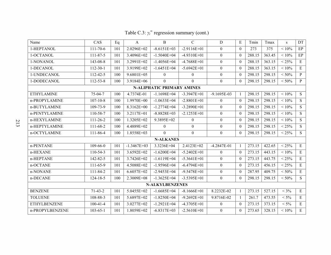
213

Table C.3: γi∞ regression summary (cont.)

Name CAS Eq A B C D E Tmin Tmax s DT 1-HEPTANOL 111-70-6 101 2.0296E+02 -8.6151E+03 -2.9116E+01 0 0 273 375 < 10% EP 1-OCTANOL 111-87-5 101 3.4096E+02 -1.5040E+04 -4.9310E+01 0 0 288.15 363.45 < 10% EP 1-NONANOL 143-08-8 101 3.2991E+02 -1.4056E+04 -4.7688E+01 0 0 288.15 363.15 < 25% E 1-DECANOL 112-30-1 101 3.9199E+02 -1.6451E+04 -5.6942E+01 0 0 288.15 363.15 < 10% E 1-UNDECANOL 112-42-5 100 9.6801E+05 0 0 0 0 298.15 298.15 < 50% P 1-DODECANOL 112-53-8 100 3.9184E+06 0 0 0 0 298.15 298.15 < 50% P

N-ALIPHATIC PRIMARY AMINES ETHYLAMINE 75-04-7 100 4.7374E-01 -1.1698E+04 -3.3947E+01 -9.1695E-03 1 298.15 298.15 < 10% S n-PROPYLAMINE 107-10-8 100 1.9970E+00 -1.0633E+04 -2.8801E+01 0 0 298.15 298.15 < 10% S n-BUTYLAMINE 109-73-9 100 8.3162E+00 -1.2774E+04 -3.2890E+01 0 0 298.15 298.15 < 10% S n-PENTYLAMINE 110-58-7 100 3.2117E+01 -8.8828E+03 -2.1253E+01 0 0 298.15 298.15 < 10% S n-HEXYLAMINE 111-26-2 100 1.3205E+02 9.3895E+02 0 0 0 298.15 298.15 < 10% S n-HEPTYLAMINE 111-68-2 100 4.4889E+02 0 0 0 0 298.15 298.15 < 25% S n-OCTYLAMINE 111-86-4 100 1.8558E+03 0 0 0 0 298.15 298.15 < 25% S

N-ALKANES n-PENTANE 109-66-0 101 -1.3467E+03 3.3236E+04 2.4123E+02 -4.2847E-01 1 273.15 422.65 < 25% E n-HEXANE 110-54-3 101 3.6592E+02 -1.6200E+04 -5.2402E+01 0 0 273.15 443.15 < 10% E n-HEPTANE 142-82-5 101 3.7426E+02 -1.6119E+04 -5.3641E+01 0 0 273.15 443.75 < 25% E n-OCTANE 111-65-9 101 4.5088E+02 -1.9596E+04 -6.4794E+01 0 0 273.15 456.15 < 25% E n-NONANE 111-84-2 101 6.6057E+02 -2.9453E+04 -9.5478E+01 0 0 287.95 409.75 < 50% E n-DECANE 124-18-5 100 2.3009E+08 -1.3625E+04 -3.5395E+01 0 0 298.15 298.15 < 50% S

N-ALKYLBENZENES BENZENE 71-43-2 101 5.0455E+02 -1.6685E+04 -8.1666E+01 8.2232E-02 1 273.15 527.15 < 3% E TOLUENE 108-88-3 101 5.6897E+02 -1.8250E+04 -9.2692E+01 9.8716E-02 1 261.7 473.55 < 5% E ETHYLBENZENE 100-41-4 101 3.0277E+02 -1.2921E+04 -4.3705E+01 0 0 273.15 373.15 < 5% E n-PROPYLBENZENE 103-65-1 101 1.8059E+02 -6.8317E+03 -2.5610E+01 0 0 273.65 328.15 < 10% E

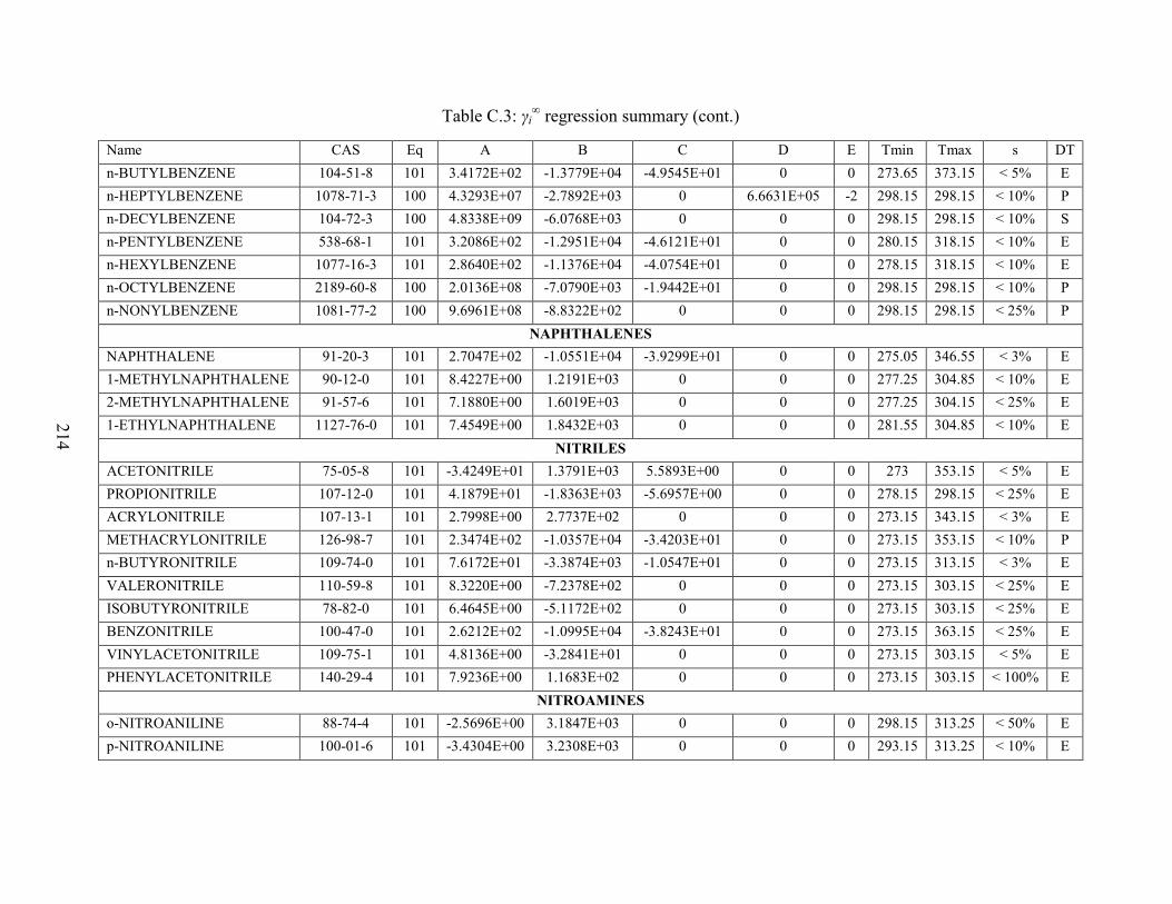
214

Table C.3: γi∞ regression summary (cont.)

Name CAS Eq A B C D E Tmin Tmax s DT n-BUTYLBENZENE 104-51-8 101 3.4172E+02 -1.3779E+04 -4.9545E+01 0 0 273.65 373.15 < 5% E n-HEPTYLBENZENE 1078-71-3 100 4.3293E+07 -2.7892E+03 0 6.6631E+05 -2 298.15 298.15 < 10% P n-DECYLBENZENE 104-72-3 100 4.8338E+09 -6.0768E+03 0 0 0 298.15 298.15 < 10% S n-PENTYLBENZENE 538-68-1 101 3.2086E+02 -1.2951E+04 -4.6121E+01 0 0 280.15 318.15 < 10% E n-HEXYLBENZENE 1077-16-3 101 2.8640E+02 -1.1376E+04 -4.0754E+01 0 0 278.15 318.15 < 10% E n-OCTYLBENZENE 2189-60-8 100 2.0136E+08 -7.0790E+03 -1.9442E+01 0 0 298.15 298.15 < 10% P n-NONYLBENZENE 1081-77-2 100 9.6961E+08 -8.8322E+02 0 0 0 298.15 298.15 < 25% P

NAPHTHALENES NAPHTHALENE 91-20-3 101 2.7047E+02 -1.0551E+04 -3.9299E+01 0 0 275.05 346.55 < 3% E 1-METHYLNAPHTHALENE 90-12-0 101 8.4227E+00 1.2191E+03 0 0 0 277.25 304.85 < 10% E 2-METHYLNAPHTHALENE 91-57-6 101 7.1880E+00 1.6019E+03 0 0 0 277.25 304.15 < 25% E 1-ETHYLNAPHTHALENE 1127-76-0 101 7.4549E+00 1.8432E+03 0 0 0 281.55 304.85 < 10% E

NITRILES ACETONITRILE 75-05-8 101 -3.4249E+01 1.3791E+03 5.5893E+00 0 0 273 353.15 < 5% E PROPIONITRILE 107-12-0 101 4.1879E+01 -1.8363E+03 -5.6957E+00 0 0 278.15 298.15 < 25% E ACRYLONITRILE 107-13-1 101 2.7998E+00 2.7737E+02 0 0 0 273.15 343.15 < 3% E METHACRYLONITRILE 126-98-7 101 2.3474E+02 -1.0357E+04 -3.4203E+01 0 0 273.15 353.15 < 10% P n-BUTYRONITRILE 109-74-0 101 7.6172E+01 -3.3874E+03 -1.0547E+01 0 0 273.15 313.15 < 3% E VALERONITRILE 110-59-8 101 8.3220E+00 -7.2378E+02 0 0 0 273.15 303.15 < 25% E ISOBUTYRONITRILE 78-82-0 101 6.4645E+00 -5.1172E+02 0 0 0 273.15 303.15 < 25% E BENZONITRILE 100-47-0 101 2.6212E+02 -1.0995E+04 -3.8243E+01 0 0 273.15 363.15 < 25% E VINYLACETONITRILE 109-75-1 101 4.8136E+00 -3.2841E+01 0 0 0 273.15 303.15 < 5% E PHENYLACETONITRILE 140-29-4 101 7.9236E+00 1.1683E+02 0 0 0 273.15 303.15 < 100% E

NITROAMINES o-NITROANILINE 88-74-4 101 -2.5696E+00 3.1847E+03 0 0 0 298.15 313.25 < 50% E p-NITROANILINE 100-01-6 101 -3.4304E+00 3.2308E+03 0 0 0 293.15 313.25 < 10% E

215

Table C.3: γi∞ regression summary (cont.)

Name CAS Eq A B C D E Tmin Tmax s DT ORGANIC SALTS

DIETHYL CARBONATE 105-58-8 101 1.8930E+02 -8.8485E+03 -2.6978E+01 0 0 273.15 363.45 < 5% E DIMETHYL CARBONATE 616-38-6 101 1.7097E+02 -7.8524E+03 -2.4703E+01 0 0 273.35 333.15 < 3% E

OTHER ALIPHATIC ALCOHOLS ISOPROPANOL 67-63-0 101 1.4959E+02 -7.7472E+03 -2.1323E+01 0 0 273 373.15 < 10% E 2-METHYL-1-PROPANOL 78-83-1 101 2.7441E+02 -1.2923E+04 -3.9876E+01 0 0 273.35 374.15 < 10% E 2-BUTANOL 78-92-2 101 1.8600E+02 -9.4446E+03 -2.6519E+01 0 0 273 371.15 < 5% E 2-METHYL-2-PROPANOL 75-65-0 101 1.6764E+02 -9.0892E+03 -2.3636E+01 0 0 273 371.15 < 10% E 2-PENTANOL 6032-29-7 101 2.1732E+02 -1.0616E+04 -3.1087E+01 0 0 273.35 371.15 < 5% E 2-METHYL-2-BUTANOL 75-85-4 101 1.7560E+02 -9.3077E+03 -2.4714E+01 0 0 273.35 371.45 < 5% E 2-METHYL-1-BUTANOL 137-32-6 101 2.5881E+02 -1.2308E+04 -3.7301E+01 0 0 273.35 363.15 < 5% E 2,2-DIMETHYL-1-PROPANOL

75-84-3 101 2.2174E+02 -1.1079E+04 -3.1540E+01 0 0 285.15 363.15 < 25% P

2-HEXANOL 626-93-7 101 2.3127E+02 -1.1094E+04 -3.2981E+01 0 0 273.15 363.35 < 25% EP 3-HEXANOL 623-37-0 101 2.2426E+02 -1.1042E+04 -3.1824E+01 0 0 273.15 363.45 < 5% EP 3-METHYL-1-PENTANOL 589-35-5 101 2.4864E+02 -1.1604E+04 -3.5685E+01 0 0 273.15 363.65 < 10% P 3-METHYL-3-PENTANOL 77-74-7 101 7.3413E+01 -4.2766E+03 -9.4714E+00 0 0 282.95 363.55 < 10% P 3-PENTANOL 584-02-1 101 2.1706E+02 -1.0682E+04 -3.1030E+01 0 0 273.35 371.15 < 5% E 3-METHYL-1-BUTANOL 123-51-3 101 3.5250E+02 -1.6416E+04 -5.1307E+01 0 0 273.35 374.15 < 10% E 3-METHYL-2-BUTANOL 598-75-4 101 2.1025E+02 -1.0387E+04 -3.0020E+01 0 0 273.35 371.15 < 3% E 2-HEPTANOL 543-49-7 101 2.5987E+02 -1.2308E+04 -3.7057E+01 0 0 273.15 363.35 < 5% P 3-HEPTANOL 589-82-2 101 2.2688E+02 -1.1106E+04 -3.2011E+01 0 0 273.15 363.35 < 10% E 4-METHYL-2-PENTANOL 108-11-2 101 1.9584E+02 -9.5636E+03 -2.7711E+01 0 0 273.15 363.35 < 10% EP 2-OCTANOL 123-96-6 101 3.7853E+02 -1.7786E+04 -5.4429E+01 0 0 273.15 363.65 < 10% P 2-NONANOL 628-99-9 101 3.8316E+02 -1.8280E+04 -5.4709E+01 0 0 273.15 363.65 < 25% P 2,6-DIMETHYL-4-HEPTANOL

108-82-7 101 1.6061E+02 -8.1347E+03 -2.1735E+01 0 0 273.15 363.65 < 25% P

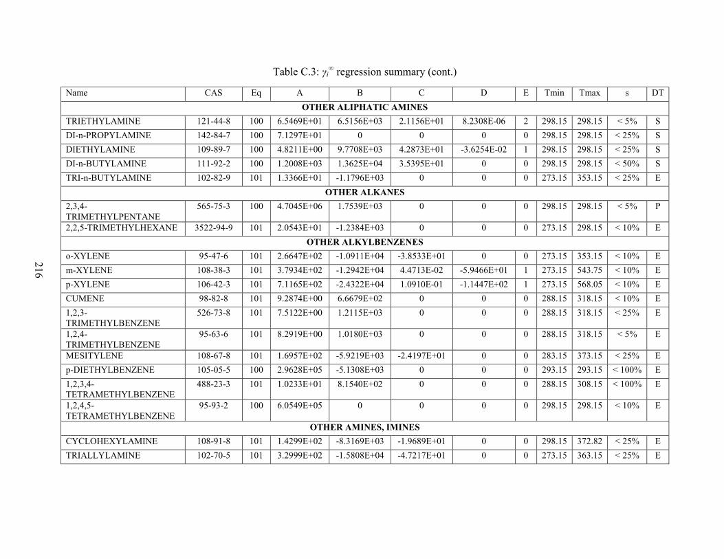
216

Table C.3: γi∞ regression summary (cont.)

Name CAS Eq A B C D E Tmin Tmax s DT OTHER ALIPHATIC AMINES

TRIETHYLAMINE 121-44-8 100 6.5469E+01 6.5156E+03 2.1156E+01 8.2308E-06 2 298.15 298.15 < 5% S DI-n-PROPYLAMINE 142-84-7 100 7.1297E+01 0 0 0 0 298.15 298.15 < 25% S DIETHYLAMINE 109-89-7 100 4.8211E+00 9.7708E+03 4.2873E+01 -3.6254E-02 1 298.15 298.15 < 25% S DI-n-BUTYLAMINE 111-92-2 100 1.2008E+03 1.3625E+04 3.5395E+01 0 0 298.15 298.15 < 50% S TRI-n-BUTYLAMINE 102-82-9 101 1.3366E+01 -1.1796E+03 0 0 0 273.15 353.15 < 25% E

OTHER ALKANES 2,3,4-TRIMETHYLPENTANE

565-75-3 100 4.7045E+06 1.7539E+03 0 0 0 298.15 298.15 < 5% P

2,2,5-TRIMETHYLHEXANE 3522-94-9 101 2.0543E+01 -1.2384E+03 0 0 0 273.15 298.15 < 10% E OTHER ALKYLBENZENES

o-XYLENE 95-47-6 101 2.6647E+02 -1.0911E+04 -3.8533E+01 0 0 273.15 353.15 < 10% E m-XYLENE 108-38-3 101 3.7934E+02 -1.2942E+04 4.4713E-02 -5.9466E+01 1 273.15 543.75 < 10% E p-XYLENE 106-42-3 101 7.1165E+02 -2.4322E+04 1.0910E-01 -1.1447E+02 1 273.15 568.05 < 10% E CUMENE 98-82-8 101 9.2874E+00 6.6679E+02 0 0 0 288.15 318.15 < 10% E 1,2,3-TRIMETHYLBENZENE

526-73-8 101 7.5122E+00 1.2115E+03 0 0 0 288.15 318.15 < 25% E

1,2,4-TRIMETHYLBENZENE

95-63-6 101 8.2919E+00 1.0180E+03 0 0 0 288.15 318.15 < 5% E

MESITYLENE 108-67-8 101 1.6957E+02 -5.9219E+03 -2.4197E+01 0 0 283.15 373.15 < 25% E p-DIETHYLBENZENE 105-05-5 100 2.9628E+05 -5.1308E+03 0 0 0 293.15 293.15 < 100% E 1,2,3,4-TETRAMETHYLBENZENE

488-23-3 101 1.0233E+01 8.1540E+02 0 0 0 288.15 308.15 < 100% E

1,2,4,5-TETRAMETHYLBENZENE

95-93-2 100 6.0549E+05 0 0 0 0 298.15 298.15 < 10% E

OTHER AMINES, IMINES CYCLOHEXYLAMINE 108-91-8 101 1.4299E+02 -8.3169E+03 -1.9689E+01 0 0 298.15 372.82 < 25% E TRIALLYLAMINE 102-70-5 101 3.2999E+02 -1.5808E+04 -4.7217E+01 0 0 273.15 363.15 < 25% E

217

Table C.3: γi∞ regression summary (cont.)

Name CAS Eq A B C D E Tmin Tmax s DT OTHER CONDENSED RINGS

FLUORANTHENE 206-44-0 101 4.0885E+00 3.6092E+03 0 0 0 281.25 333.15 < 10% E FLUORENE 86-73-7 101 3.8046E+00 3.0197E+03 0 0 0 279.75 333.15 < 10% E ANTHRACENE 120-12-7 101 2.8549E+02 -2.0510E+04 -3.8180E+01 0 0 273.45 347.85 < 5% E PHENANTHRENE 85-01-8 101 2.4635E+02 -7.8027E+03 -3.6051E+01 0 0 277.15 346.55 < 5% E CHRYSENE 218-01-9 101 1.0112E+01 2.7117E+03 0 0 0 279.65 302.15 < 25% E PYRENE 129-00-0 101 2.8752E+02 -9.6725E+03 -4.1927E+01 0 0 277.85 347.85 < 5% E ACENAPHTHENE 83-32-9 101 4.2310E+00 2.6602E+03 0 0 0 277.25 347.85 < 25% E ACENAPHTHALENE 208-96-8 101 6.4639E+00 1.9187E+03 0 0 0 277.25 304.15 < 25% E BENZO[a]PYRENE 50-32-8 101 7.4109E+00 4.1135E+03 0 0 0 281.15 308.15 < 10% E BENZO[b]FLUORANTHENE 205-99-2 101 -2.0161E+00 6.3942E+03 0 0 0 283.15 328.15 < 10% E

OTHER ETHERS/DIETHERS METHYLAL 109-87-5 101 6.6045E+00 -1.1224E+03 0 0 0 273.35 333.15 < 25% E 1,2-DIMETHOXYETHANE 110-71-4 101 1.9979E+02 -1.1271E+04 -2.8177E+01 0 0 273.35 372.5 < 3% E DIETHYLENE GLYCOL DI-n-BUTYL ETHER

112-73-2 101 2.5849E+01 -5.0993E+03 0 0 0 273.15 293.15 < 100% P

ANISOLE 100-66-3 101 3.7640E+00 1.3538E+03 0 0 0 275.15 363.85 < 5% E DIPHENYL ETHER 101-84-8 100 4.9071E+05 0 0 0 0 298.15 298.15 < 50% S

OTHER INORGANICS HYDROGEN PEROXIDE 7722-84-1 101 1.1957E+00 -8.0509E+02 0 0 0 278.15 297.15 < 25% E

OTHER MONOAROMATICS STYRENE 100-42-5 101 4.1793E+00 1.6920E+03 0 0 0 293.32 313.02 < 5% E

OTHER POLYFUNCTIONAL C, H, O 2-BUTOXYETHANOL 111-76-2 101 8.7199E+00 -1.5162E+03 0 0 0 293.15 303.15 < 25% E VANILLIN 121-33-5 101 -4.5897E+02 2.2705E+04 6.8209E+01 0 0 293.15 318.15 < 5% E

218

Table C.3: γi∞ regression summary (cont.)

Name CAS Eq A B C D E Tmin Tmax s DT OTHER POLYFUNCTIONAL ORGANICS

MALATHION 121-75-5 101 9.4811E+00 6.5738E+02 0 0 0 283.15 303.15 < 25% E OTHER SATURATED ALIPHATIC ESTERS

ETHYL ISOVALERATE 108-64-5 101 1.9687E+02 -9.4132E+03 -2.7576E+01 0 0 273.15 363.65 < 10% E DIETHYL MALONATE 105-53-3 101 2.1777E+02 -1.0033E+04 -3.1264E+01 0 0 273.15 363.75 < 10% P ETHYL TRIMETHYL ACETATE

3938-95-2 101 1.7393E+02 -8.6446E+03 -2.3987E+01 0 0 273.15 363.55 < 25% E

PEROXIDES METHYL HYDROPEROXIDE

3031-73-0 101 1.0534E+00 7.9863E+01 0 0 0 277.15 297.15 < 3% E

ETHYL HYDROPEROXIDE 3031-74-1 101 2.7406E+00 -3.6257E+02 0 0 0 278.15 297.15 < 10% E POLYFUNCTIONAL AMIDES/AMINES

N,N-DIMETHYLFORMAMIDE

68-12-2 101 1.4648E+02 -8.3423E+03 -2.0868E+01 0 0 289.4 372 < 25% E

N-METHYLFORMAMIDE 123-39-7 101 2.0381E+00 -5.8045E+02 0 0 0 333.15 372.65 < 5% E N,N-DIMETHYLACETAMIDE

127-19-5 101 7.5170E+00 -2.4924E+03 0 0 0 343.15 372.28 < 10% E

POLYFUNCTIONAL C, H, N, HALIDE, (O) o-CHLOROANILINE 95-51-2 101 1.2561E+03 -4.1122E+04 -2.0798E+02 2.4659E-01 1 298.15 431.15 < 25% P p-CHLORONITROBENZENE

100-00-5 101 2.1438E+00 2.3385E+03 0 0 0 283.15 313.15 < 10% E

POLYFUNCTIONAL C, H, O, HALIDE DI(2-CHLOROETHYL)ETHER

111-44-4 101 1.5144E+02 -6.4595E+03 -2.1611E+01 0 0 273.15 364.85 < 5% E

ETHYLCHLOROACETATE 105-39-5 101 1.9772E+02 -8.9873E+03 -2.8391E+01 0 0 273.15 333.25 < 10% E METHYL CHLOROACETATE

96-34-4 101 1.0528E+02 -4.4693E+03 -1.5019E+01 0 0 273.15 323.35 < 5% E

POLYFUNCTIONAL C, H, O, N N-METHYL-2-PYRROLIDONE

872-50-4 101 3.9967E+02 -2.1700E+04 -5.7549E+01 0 0 298.8 372.85 < 5% E

219

Table C.3: γi∞ regression summary (cont.)

Name CAS Eq A B C D E Tmin Tmax s DT POLYFUNCTIONAL C, H, O, S

DIMETHYL SULFOXIDE 67-68-5 101 2.9405E+00 -1.6085E+03 0 0 0 298.8 337.9 < 25% E POLYFUNCTIONAL ESTERS

METHYL SALICYLATE 119-36-8 101 1.6195E+02 -6.2843E+03 -2.3185E+01 0 0 273.15 363.65 < 25% E 2-ETHOXYETHYL ACETATE

111-15-9 100 4.7700E+01 0 0 0 0 303.15 303.15 < 10% E

ETHYL ACETOACETATE 141-97-9 101 6.4902E+00 -6.8868E+02 0 0 0 273.15 303.15 < 25% EP ETHYLENE GLYCOL MONOBUTYL ETHER ACETATE

112-07-2 100 2.6459E+02 0 0 0 0 298.15 298.15 < 25% E

PROPIONATES AND BUTYRATES METHYL PROPIONATE 554-12-1 101 8.7616E+00 -1.2878E+03 0 0 0 273.15 310.2 < 5% E ETHYL PROPIONATE 105-37-3 101 2.3017E+02 -1.0936E+04 -3.2963E+01 0 0 273.15 353.45 < 25% E n-PROPYL PROPIONATE 106-36-5 101 1.7662E+02 -8.7139E+03 -2.4641E+01 0 0 273.15 363.65 < 10% E n-BUTYL PROPIONATE 590-01-2 101 2.1594E+02 -1.0309E+04 -3.0373E+01 0 0 273.15 363.55 < 10% E n-PROPYL n-BUTYRATE 105-66-8 101 2.0811E+02 -9.7622E+03 -2.9327E+01 0 0 273.15 363.65 < 25% E METHYL n-BUTYRATE 623-42-7 101 1.0572E+02 -5.2463E+03 -1.4460E+01 0 0 273.15 363.65 < 25% E ETHYL n-BUTYRATE 105-54-4 101 1.4646E+02 -7.2997E+03 -2.0200E+01 0 0 273.15 363.65 < 25% E ISOBUTYL ISOBUTYRATE 97-85-8 101 2.2011E+02 -1.0408E+04 -3.0834E+01 0 0 273.15 363.45 < 25% E n-BUTYL n-BUTYRATE 109-21-7 101 2.9628E+02 -1.4154E+04 -4.2014E+01 0 0 273.15 363.45 < 10% E METHYL ISOBUTYRATE 547-63-7 101 1.4441E+02 -7.0836E+03 -2.0168E+01 0 0 273.15 353.45 < 10% E ETHYL ISOBUTYRATE 97-62-1 101 1.4146E+02 -7.0790E+03 -1.9442E+01 0 0 273.15 363.75 < 10% P n-PENTYL n-BUTYRATE 540-18-1 101 1.1097E+01 -2.1866E+02 0 0 0 273.15 363.65 < 25% E ISOPENTYL BUTYRATE 106-27-4 101 2.4293E+02 -1.1495E+04 -3.4028E+01 0 0 282.55 363.85 < 100% E

SULFIDES/THIOPHENES DIMETHYL SULFIDE 75-18-3 101 1.6724E+02 -7.3055E+03 -2.4157E+01 0 0 272.35 353.45 < 10% E DIMETHYL DISULFIDE 624-92-0 101 4.5046E+00 8.8438E+02 0 0 0 273.2 343.15 < 10% E

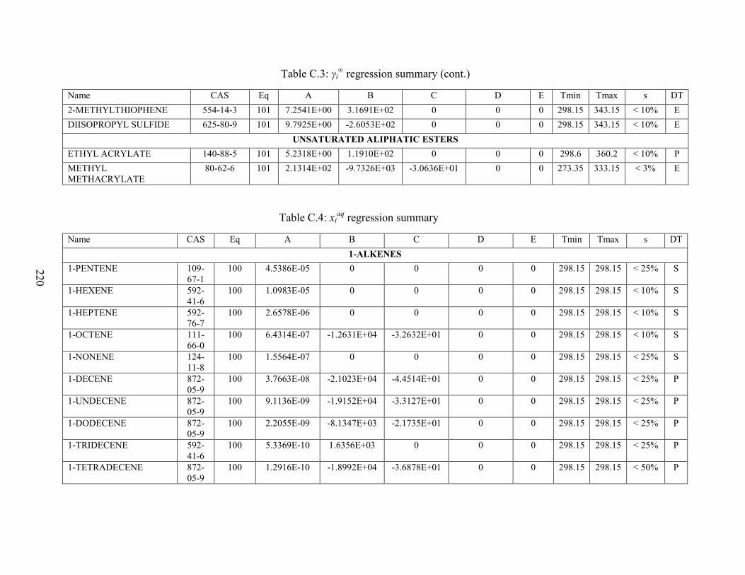
220

Table C.3: γi∞ regression summary (cont.)

Name CAS Eq A B C D E Tmin Tmax s DT 2-METHYLTHIOPHENE 554-14-3 101 7.2541E+00 3.1691E+02 0 0 0 298.15 343.15 < 10% E DIISOPROPYL SULFIDE 625-80-9 101 9.7925E+00 -2.6053E+02 0 0 0 298.15 343.15 < 10% E

UNSATURATED ALIPHATIC ESTERS ETHYL ACRYLATE 140-88-5 101 5.2318E+00 1.1910E+02 0 0 0 298.6 360.2 < 10% P METHYL METHACRYLATE

80-62-6 101 2.1314E+02 -9.7326E+03 -3.0636E+01 0 0 273.35 333.15 < 3% E

Table C.4: xiaq regression summary (cont.)

Name CAS Eq A B C D E Tmin Tmax s DT 1-ALKENES

1-PENTENE 109-67-1

100 4.5386E-05 0 0 0 0 298.15 298.15 < 25% S

1-HEXENE 592-41-6

100 1.0983E-05 0 0 0 0 298.15 298.15 < 10% S

1-HEPTENE 592-76-7

100 2.6578E-06 0 0 0 0 298.15 298.15 < 10% S

1-OCTENE 111-66-0

100 6.4314E-07 -1.2631E+04 -3.2632E+01 0 0 298.15 298.15 < 10% S

1-NONENE 124-11-8

100 1.5564E-07 0 0 0 0 298.15 298.15 < 25% S

1-DECENE 872-05-9

100 3.7663E-08 -2.1023E+04 -4.4514E+01 0 0 298.15 298.15 < 25% P

1-UNDECENE 872-05-9

100 9.1136E-09 -1.9152E+04 -3.3127E+01 0 0 298.15 298.15 < 25% P

1-DODECENE 872-05-9

100 2.2055E-09 -8.1347E+03 -2.1735E+01 0 0 298.15 298.15 < 25% P

1-TRIDECENE 592-41-6

100 5.3369E-10 1.6356E+03 0 0 0 298.15 298.15 < 25% P

1-TETRADECENE 872-05-9

100 1.2916E-10 -1.8992E+04 -3.6878E+01 0 0 298.15 298.15 < 50% P

221

Table C.4: xiaq regression summary (cont.)

Name CAS Eq A B C D E Tmin Tmax s DT 1-PENTADECENE 13360-

61-7 100 3.1253E-11 0 0 0 0 298.15 298.15 < 50% S

2,3,4-ALKENES cis-2-PENTENE 627-

20-3 100 5.2143E-05 0 0 0 0 298.15 298.15 < 5% E

trans-2-PENTENE 646-04-8

100 5.2143E-05 0 0 0 0 298.15 298.15 < 5% E

cis-2-HEPTENE 6443-92-1

100 2.7522E-06 0 0 0 0 298.15 298.15 < 10% E

trans-2-HEPTENE 14686-13-6

100 2.7522E-06 0 0 0 0 298.15 298.15 < 10% E

ACETATES METHYL ACETATE 79-20-

9 101 -2.3084E+03 1.9554E+05 3.1910E+02 -1.4952E+07 -2 278.15 356.65 < 3% E

ETHYL ACETATE 141-78-6

101 -1.3361E+03 1.0978E+05 1.8495E+02 -7.9991E+06 -2 273.15 343.65 < 3% E

n-PROPYL ACETATE 109-60-4

101 4.8913E+00 -7.2626E+03 0 1.2351E+06 -2 273.15 363.35 < 5% E

n-BUTYL ACETATE 123-86-4

101 3.1799E+00 -6.9848E+03 0 1.1870E+06 -2 273.15 363.65 < 10% E

ISOBUTYL ACETATE 110-19-0

101 8.7151E+00 -1.0152E+04 0 1.6438E+06 -2 273.15 420.25 < 10% E

ISOPENTYL ACETATE 123-92-2

101 6.9823E+00 -1.0058E+04 0 1.6541E+06 -2 273.15 363.85 < 10% E

ISOPROPYL ACETATE 108-21-4

101 6.2087E+00 -8.1630E+03 0 1.4057E+06 -2 273.15 366.15 < 10% E

sec-BUTYL ACETATE 105-46-4

101 3.8824E+00 -7.4666E+03 0 1.2842E+06 -2 273.15 363.65 < 10% E

VINYL ACETATE 108-05-4

101 3.3355E+00 -5.4481E+03 0 8.6465E+05 -2 273.35 333.15 < 3% E

n-PENTYL ACETATE 628-63-7

101 1.3007E+01 -1.4017E+04 0 2.2856E+06 -2 273.15 364.5 < 25% E

n-HEXYL ACETATE 142-92-7

101 1.7463E+01 -1.7134E+04 0 2.6915E+06 -2 273.15 363.35 < 25% E

222

Table C.4: xiaq regression summary (cont.)

Name CAS Eq A B C D E Tmin Tmax s DT n-HEPTYL ACETATE 112-

06-1 100 1.5184E-05 -1.5368E+04 -3.7557E+01 0 0 298.15 298.15 < 25% P

n-OCTYL ACETATE 112-14-1

100 3.7799E-06 -1.1079E+04 -3.1540E+01 0 0 298.15 298.15 < 25% P

ETHYLENE GLYCOL DIACETATE

111-55-7

101 6.4818E+00 -6.0277E+03 0 8.8752E+05 -2 273.15 363.25 < 3% E

tert-BUTYL ACETATE 540-88-5

101 1.3823E+00 -6.1464E+03 0 1.1073E+06 -2 273.15 353.65 < 3% E

CYCLOHEXYL ACETATE

622-45-7

101 4.5951E+00 -8.3650E+03 0 1.3772E+06 -2 273.15 363.45 < 10% E

PHENYL ACETATE 122-79-2

101 6.0837E+00 -7.8765E+03 0 1.1694E+06 -2 273.15 363.95 < 10% E

ALDEHYDES ACETALDEHYDE 75-07-

0 101 -2.0000E+01 5.5703E+03 0 0 0 294.15 318.15 < 10% P

PROPANAL 123-38-6

101 -1.0158E+01 2.4071E+03 0 0 0 285.45 323.15 < 25% E

BUTANAL 123-72-8

101 -9.0064E+00 1.4733E+03 0 0 0 273.15 343.15 < 10% E

2-METHYLPROPANAL 78-84-2

101 -8.9679E+00 1.3843E+03 0 0 0 273.15 333.15 < 5% E

PENTANAL 110-62-3

101 -9.8645E+00 1.2720E+03 0 0 0 273.15 363.15 < 50% E

HEPTANAL 111-71-7

101 1.5461E+01 -1.5603E+04 0 2.5355E+06 -2 273.15 363.15 < 10% E

HEXANAL 66-25-1

101 1.7602E+01 -1.6591E+04 0 2.7535E+06 -2 273.15 373.15 < 25% E

OCTANAL 124-13-0

101 -1.3858E+01 1.2453E+03 0 0 0 283.15 318.15 < 50% E

NONANAL 124-19-6

101 -8.9336E+00 -8.6592E+02 0 0 0 283.15 318.15 < 50% E

2-ETHYLHEXANAL 123-05-7

101 -8.2417E+00 -4.5642E+02 0 0 0 273.15 363.15 < 25% E

223

Table C.4: xiaq regression summary (cont.)

Name CAS Eq A B C D E Tmin Tmax s DT 2-ETHYL-2-HEXENAL 645-

62-5 101 -8.3157E+00 -1.0075E+02 0 0 0 273.15 363.15 < 25% E

DECANAL 112-31-2

101 -1.6848E+01 1.0170E+03 0 0 0 298.15 318.15 < 50% E

2-METHYL-BUTYRALDEHYDE

96-17-3

101 -9.8239E+00 1.2190E+03 0 0 0 273.15 363.15 < 25% E

ACROLEIN 107-02-8

5000 -1.0495E+04 6.6687E+04 1.5256E+03 1.3239E+03 361.35 273.15 361.15 < 10% E

trans-CROTONALDEHYDE

123-73-9

101 4.1230E+00 -4.8483E+03 0 8.0558E+05 -2 273.15 363.15 < 10% E

METHACROLEIN 78-85-3

101 -6.5100E+00 7.1224E+02 0 0 0 273.15 333.15 < 10% E

p-TOLUALDEHYDE 104-87-0

101 -5.9618E+00 -6.6380E+02 0 0 0 273.15 363.15 < 10% E

BENZALDEHYDE 100-52-7

101 1.1413E+01 -1.0321E+04 0 1.4635E+06 -2 273.08 373.15 < 10% E

ALIPHATIC ETHERS DIETHYL ETHER 60-29-

7 101 -1.2269E+01 2.4068E+03 0 0 0 269.32 307.25 < 5% E

DIISOPROPYL ETHER 108-20-3

101 -1.9779E+01 5.2627E+03 0 -3.8263E+05 -2 273.15 334.15 < 10% E

DI-n-BUTYL ETHER 142-96-1

101 -1.5032E+01 1.3926E+03 0 0 0 273.15 363.65 < 25% E

METHYL tert-BUTYL ETHER

1634-04-4

101 -8.9827E+00 2.3199E+02 0 3.0025E+05 -2 273.15 343.15 < 10% E

METHYL ISOBUTYL ETHER

625-44-5

101 -1.5502E+01 2.8024E+03 0 0 0 273.15 298.15 < 5% E

DI-n-HEXYL ETHER 112-58-3

100 6.8917E-08 -3.2876E+04 -7.4441E+01 0 0 298.15 298.15 < 25% P

METHYL n-BUTYL ETHER

628-28-4

101 -1.8085E+01 3.4942E+03 0 0 0 273.15 298.15 < 25% E

DI-n-PENTYL ETHER 693-65-2

100 2.2173E-06 -1.2187E+03 0 0 0 298.15 298.15 < 25% P

224

Table C.4: xiaq regression summary (cont.)

Name CAS Eq A B C D E Tmin Tmax s DT METHYL tert-PENTYL ETHER

994-05-8

101 -1.4359E+00 -5.3257E+03 0 1.1530E+06 -2 273.15 352.35 < 10% E

tert-BUTYL ETHYL ETHER

637-92-3

101 -1.5992E+01 2.9990E+03 0 0 0 278.15 318.15 < 25% E

ETHYL tert-PENTYL ETHER

919-94-8

101 -1.7642E+01 2.9896E+03 0 0 0 288.15 318.15 < 25% E

DI-n-PROPYL ETHER 111-43-3

101 1.4439E+01 -1.5271E+04 0 2.5850E+06 -2 273.15 333.25 < 10% E

n-BUTYL ETHYL ETHER

628-81-9

101 5.5361E+00 -8.7602E+03 0 1.5059E+06 -2 273.15 363.85 < 25% E

ALKYLCYCLOHEXANES METHYL-CYCLOHEXANE

108-87-2

101 2.2613E+01 -2.1770E+04 0 3.3465E+06 -2 293.15 443.95 < 25% E

ETHYL-CYCLOHEXANE 1678-91-7

101 5.7107E+02 -6.9022E+04 -7.5554E+01 6.8089E+06 -2 274.15 443.95 < 10% E

cis-1,2-DIMETHYL-CYCLOHEXANE

2207-01-4

101 9.2417E+00 -1.3497E+04 0 1.9708E+06 -2 274.15 313.15 < 3% E

trans-1,2-DIMETHYL-CYCLOHEXANE

6876-23-9

101 4.0532E+02 -5.4401E+04 -5.2782E+01 5.6689E+06 -2 274.15 443.25 < 5% E

ALKYL-CYCLOPENTANES

METHYL-CYCLOPENTANE

96-37-7

100 9.1506E-06 -1.3517E+04 -3.1894E+01 0 0 298.15 298.15 < 3% S

ALKYNES ETHYLACETYLENE 107-

00-6 100 1.0280E-03 0 0 0 0 298.15 298.15 < 25% S

1-PENTYNE 627-19-0

100 4.0450E-04 0 0 0 0 298.15 298.15 < 25% S

1-HEXYNE 693-02-7

100 8.4660E-05 0 0 0 0 298.15 298.15 < 25% S

1-OCTYNE 629-05-0

100 3.9470E-06 0 0 0 0 298.15 298.15 < 25% S

1-NONYNE 3452-09-3

100 7.6320E-07 0 0 0 0 298.15 298.15 < 25% S

225

Table C.4: xiaq regression summary (cont.)

Name CAS Eq A B C D E Tmin Tmax s DT 1-HEPTYNE 628-

71-7 100 1.8240E-05 0 0 0 0 298.15 298.15 < 25% S

AROMATIC ALCOHOLS 2,3-XYLENOL 526-

75-0 6000 -1.5683E+01 1.6800E+03 2.0352E-02 -4.5266E+00 483.26 293.15 483.25 < 25% E

2,4-XYLENOL 105-67-9

6000 -2.3457E+01 3.2524E+03 2.8887E-02 -3.8002E+00 486.06 298.15 486.05 < 25% E

2,5-XYLENOL 95-87-4

6000 1.1654E+01 -3.1846E+03 -1.4892E-02 -5.5852E+00 492.16 293.15 492.15 < 25% E

2,6-XYLENOL 576-26-1

6000 -2.9019E+01 4.1106E+03 3.6790E-02 -3.6459E+00 514.35 293.15 514.35 < 25% E

3,4-XYLENOL 95-65-8

6000 -1.4145E+00 -4.9478E+02 1.1971E-04 -5.6703E+00 463.36 293.15 463.35 < 25% E

3,5-XYLENOL 108-68-9

6000 3.1997E+00 -1.1427E+03 -6.1815E-03 -6.5122E+00 473.16 293.15 473.15 < 25% E

BENZYL ALCOHOL 100-51-6

6000 -1.7550E+01 2.6630E+03 2.1755E-02 -4.1474E+00 421.66 273.15 421.65 < 10% E

PHENOL 108-95-2

6000 -2.6083E+01 4.1611E+03 3.5914E-02 -5.3947E+00 341.46 273.15 341.45 < 10% E

o-CRESOL 95-48-7

6000 -5.1769E+00 6.8531E+02 4.0436E-03 -5.4711E+00 439.66 273.15 439.65 < 25% E

m-CRESOL 108-39-4

6000 -6.2483E+00 8.1278E+02 5.3851E-03 -5.4723E+00 421.86 272.95 421.85 < 10% E

p-CRESOL 106-44-5

6000 1.3914E+01 -2.4840E+03 -2.4577E-02 -6.0623E+00 416.86 273.15 416.85 < 10% E

p-ETHYLPHENOL 123-07-9

6000 -9.4585E+00 1.6912E+03 7.9368E-03 -7.7616E+00 460.26 298.15 460.25 < 50% E

2-PHENYLETHANOL 60-12-8

101 1.0118E+01 -9.3144E+03 0 1.3785E+06 -2 283.15 373.15 < 10% E

1-PHENYL-1-PROPANOL

93-54-9

101 8.8268E+00 -9.9590E+03 0 1.5984E+06 -2 293.15 363.65 < 5% E

AROMATIC AMINES o-TOLUIDINE 95-53-

4 101 -5.6696E+00 -4.1271E+01 0 0 0 298.15 323.15 < 25% E

226

Table C.4: xiaq regression summary (cont.)

Name CAS Eq A B C D E Tmin Tmax s DT m-TOLUIDINE 108-

44-1 101 -5.6334E+00 -9.0608E+01 0 0 0 298.15 323.15 < 25% E

p-TOLUIDINE 106-49-0

101 6.4902E+00 -3.8937E+03 0 0 0 293.15 313.15 < 5% E

QUINOLINE 91-22-5

101 -6.5531E+02 5.0239E+04 9.1044E+01 -3.4520E+06 -2 273.15 498.2 < 25% E

N,N-DIETHYLANILINE 91-66-7

101 -9.3555E+00 -4.0851E+02 0 0 0 273.15 333.15 < 10% E

PYRIDINE 110-86-1

100 1 0 0 0 0 273.15 368.15 U E

ANILINE 62-53-3

101 7.6638E+00 -7.1200E+03 0 1.0031E+06 -2 281.75 369.85 < 3% E

2-METHYLPYRIDINE 109-06-8

100 1 0 0 0 0 273.15 368.15 U E

o-ETHYLANILINE 578-54-1

101 5.2059E+00 -7.4833E+03 0 1.1569E+06 -2 283.15 363.15 < 10% E

2,4,6-TRIMETHYL-PYRIDINE

108-75-8

6000 -2.4933E+01 3.0991E+03 3.6399E-02 -4.2595E+00 279.64 279.65 363.15 < 25% E

2,6-DIMETHYL-PYRIDINE

108-48-5

6000 -5.0882E+01 7.5209E+03 7.6927E-02 -4.9826E+00 307.14 307.15 363.15 < 10% E

3-METHYLPYRIDINE 108-99-6

100 1 0 0 0 0 273.15 368.15 U E

4-METHYL-PYRIDINE 108-89-4

100 1 0 0 0 0 273.15 368.15 U E

2,4-DIMETHYL-ANILINE

95-68-1

101 1.2321E+01 -1.2131E+04 0 1.8891E+06 -2 273.15 363.15 < 10% E

N-ETHYLANILINE 103-69-5

101 7.1042E+00 -9.4288E+03 0 1.4841E+06 -2 273.15 363.15 < 5% E

AROMATIC CARBOXYLIC ACIDS o-TOLUIC ACID 118-

90-1 6000 1.5306E+00 -2.9748E+03 6.5706E-03 -3.3513E+00 434.36 278.15 434.35 < 25% E

p-TOLUIC ACID 99-94-5

101 2.0163E+01 -1.4966E+04 0 1.7837E+06 -2 278.15 343.15 < 5% E

227

Table C.4: xiaq regression summary (cont.)

Name CAS Eq A B C D E Tmin Tmax s DT PHTHALIC ACID 88-99-

3 101 -3.2559E+03 2.8099E+05 4.4935E+02 -2.2581E+07 -2 283.65 352.45 < 5% E

m-TOLUIC ACID 99-04-7

101 2.4555E+01 -1.6880E+04 0 2.0431E+06 -2 278.15 348.15 < 3% E

AROMATIC CHLORIDES BENZYL CHLORIDE 100-

44-7 101 -4.8047E+00 -1.4232E+03 0 0 0 277.65 303.15 < 25% E

MONO-CHLOROBENZENE

108-90-7

101 1.9378E+01 -1.6010E+04 0 2.2051E+06 -2 274.15 353.16 < 10% E

o-DICHLOROBENZENE 95-50-1

101 4.6100E+01 -3.3265E+04 0 4.8466E+06 -2 278.15 318.15 < 10% E

m-DICHLOROBENZENE 541-73-1

101 -7.2884E+00 -1.1202E+03 0 0 0 278.15 318.15 < 10% E

p-DICHLOROBENZENE 106-46-7

101 1.9920E+01 -1.6897E+04 0 2.2424E+06 -2 278.15 346.55 < 10% E

HEXACHLORO-BENZENE

118-74-1

101 -8.8149E+00 -3.8499E+03 0 0 0 278.15 318.15 < 25% E

o-CHLOROTOLUENE 95-49-8

101 -7.5182E+00 -1.0005E+03 0 0 0 274.15 318.15 < 25% E

p-CHLOROTOLUENE 106-43-4

101 -7.6410E+00 -9.8024E+02 0 0 0 278.15 318.15 < 25% E

2,4-DICHLOROTOLUENE

95-73-8

101 -8.0197E+00 -1.4022E+03 0 0 0 278.15 323.1 < 10% E

1,2,4-TRICHLORO-BENZENE

120-82-1

101 -7.9726E+00 -1.3232E+03 0 0 0 278.15 318.15 < 25% E

1,2,3-TRICHLORO-BENZENE

87-61-6

101 -1.3063E+00 -3.5211E+03 0 0 0 277.15 323.15 < 25% E

AROMATIC ESTERS BENZYL ACETATE 140-

11-4 101 4.7216E+00 -7.2941E+03 0 1.0365E+06 -2 273.15 363.55 < 10% E

DI-n-PROPYL PHTHALATE

131-16-8

100 6.6314E-06 0 0 0 0 298.15 298.15 < 25% S

DI-n-HEXYL PHTHALATE

84-75-3

100 1.2643E-08 0 0 0 0 298.15 298.15 < 50% S

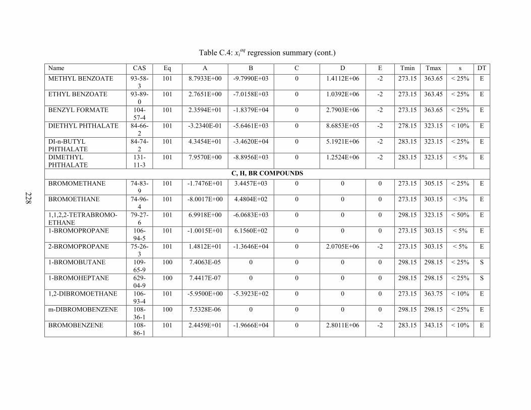
228

Table C.4: xiaq regression summary (cont.)

Name CAS Eq A B C D E Tmin Tmax s DT METHYL BENZOATE 93-58-

3 101 8.7933E+00 -9.7990E+03 0 1.4112E+06 -2 273.15 363.65 < 25% E

ETHYL BENZOATE 93-89-0

101 2.7651E+00 -7.0158E+03 0 1.0392E+06 -2 273.15 363.45 < 25% E

BENZYL FORMATE 104-57-4

101 2.3594E+01 -1.8379E+04 0 2.7903E+06 -2 273.15 363.65 < 25% E

DIETHYL PHTHALATE 84-66-2

101 -3.2340E-01 -5.6461E+03 0 8.6853E+05 -2 278.15 323.15 < 10% E

DI-n-BUTYL PHTHALATE

84-74-2

101 4.3454E+01 -3.4620E+04 0 5.1921E+06 -2 283.15 323.15 < 25% E

DIMETHYL PHTHALATE

131-11-3

101 7.9570E+00 -8.8956E+03 0 1.2524E+06 -2 283.15 323.15 < 5% E

C, H, BR COMPOUNDS BROMOMETHANE 74-83-

9 101 -1.7476E+01 3.4457E+03 0 0 0 273.15 305.15 < 25% E

BROMOETHANE 74-96-4

101 -8.0017E+00 4.4804E+02 0 0 0 273.15 303.15 < 3% E

1,1,2,2-TETRABROMO-ETHANE

79-27-6

101 6.9918E+00 -6.0683E+03 0 0 0 298.15 323.15 < 50% E

1-BROMOPROPANE 106-94-5

101 -1.0015E+01 6.1560E+02 0 0 0 273.15 303.15 < 5% E

2-BROMOPROPANE 75-26-3

101 1.4812E+01 -1.3646E+04 0 2.0705E+06 -2 273.15 303.15 < 5% E

1-BROMOBUTANE 109-65-9

100 7.4063E-05 0 0 0 0 298.15 298.15 < 25% S

1-BROMOHEPTANE 629-04-9

100 7.4417E-07 0 0 0 0 298.15 298.15 < 25% S

1,2-DIBROMOETHANE 106-93-4

101 -5.9500E+00 -5.3923E+02 0 0 0 273.15 363.75 < 10% E

m-DIBROMOBENZENE 108-36-1

100 7.5328E-06 0 0 0 0 298.15 298.15 < 25% E

BROMOBENZENE 108-86-1

101 2.4459E+01 -1.9666E+04 0 2.8011E+06 -2 283.15 343.15 < 10% E

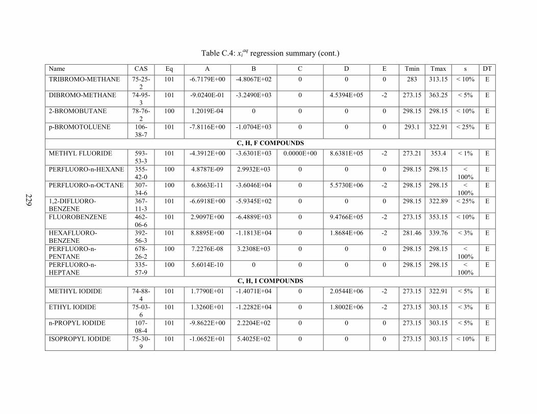
229

Table C.4: xiaq regression summary (cont.)

Name CAS Eq A B C D E Tmin Tmax s DT TRIBROMO-METHANE 75-25-

2 101 -6.7179E+00 -4.8067E+02 0 0 0 283 313.15 < 10% E

DIBROMO-METHANE 74-95-3

101 -9.0240E-01 -3.2490E+03 0 4.5394E+05 -2 273.15 363.25 < 5% E

2-BROMOBUTANE 78-76-2

100 1.2019E-04 0 0 0 0 298.15 298.15 < 10% E

p-BROMOTOLUENE 106-38-7

101 -7.8116E+00 -1.0704E+03 0 0 0 293.1 322.91 < 25% E

C, H, F COMPOUNDS METHYL FLUORIDE 593-

53-3 101 -4.3912E+00 -3.6301E+03 0.0000E+00 8.6381E+05 -2 273.21 353.4 < 1% E

PERFLUORO-n-HEXANE 355-42-0

100 4.8787E-09 2.9932E+03 0 0 0 298.15 298.15 < 100%

E

PERFLUORO-n-OCTANE 307-34-6

100 6.8663E-11 -3.6046E+04 0 5.5730E+06 -2 298.15 298.15 < 100%

E

1,2-DIFLUORO-BENZENE

367-11-3

101 -6.6918E+00 -5.9345E+02 0 0 0 298.15 322.89 < 25% E

FLUOROBENZENE 462-06-6

101 2.9097E+00 -6.4889E+03 0 9.4766E+05 -2 273.15 353.15 < 10% E

HEXAFLUORO-BENZENE

392-56-3

101 8.8895E+00 -1.1813E+04 0 1.8684E+06 -2 281.46 339.76 < 3% E

PERFLUORO-n-PENTANE

678-26-2

100 7.2276E-08 3.2308E+03 0 0 0 298.15 298.15 < 100%

E

PERFLUORO-n-HEPTANE

335-57-9

100 5.6014E-10 0 0 0 0 298.15 298.15 < 100%

E

C, H, I COMPOUNDS METHYL IODIDE 74-88-

4 101 1.7790E+01 -1.4071E+04 0 2.0544E+06 -2 273.15 322.91 < 5% E

ETHYL IODIDE 75-03-6

101 1.3260E+01 -1.2282E+04 0 1.8002E+06 -2 273.15 303.15 < 3% E

n-PROPYL IODIDE 107-08-4

101 -9.8622E+00 2.2204E+02 0 0 0 273.15 303.15 < 5% E

ISOPROPYL IODIDE 75-30-9

101 -1.0652E+01 5.4025E+02 0 0 0 273.15 303.15 < 10% E

230

Table C.4: xiaq regression summary (cont.)

Name CAS Eq A B C D E Tmin Tmax s DT IODOBENZENE 591-

50-4 101 1.7033E+01 -8.3179E+03 0 0 0 298 303.15 < 10% E

n-HEXYL IODIDE 638-45-9

100 1.1954E-06 0 0 0 0 298.15 298.15 < 25% S

n-BUTYL IODIDE 542-69-8

100 2.2740E-05 1.2631E+04 3.2632E+01 0 0 298.15 298.15 < 10% S

C, H, MULTIHALOGEN COMPOUNDS DICHLORODIFLUORO-METHANE

75-71-8

101 -4.7872E+02 3.0993E+04 6.6398E+01 -1.1878E+06 -2 274 313.9 < 3% E

TRICHLOROFLUORO-METHANE

75-69-4

1,1,2-TRICHLORO-TRIFLUOROETHANE

76-13-1

101 -1.2463E+01 5.4155E+02 0 0 0 275.15 303.15 < 25% E

C, H, NO2 COMPOUNDS NITROMETHANE 75-52-

5 101 1.5480E+01 -1.0523E+04 0 1.4556E+06 -2 273.15 363.15 < 10% E

NITROETHANE 79-24-3

101 5.9340E+00 -5.9512E+03 0 8.4315E+05 -2 273.15 363.25 < 5% E

1-NITROPROPANE 108-03-2

101 6.2988E+00 -7.1087E+03 0 1.0499E+06 -2 273.15 363.65 < 10% E

2-NITROPROPANE 79-46-9

101 4.1019E+00 -5.7427E+03 0 8.4502E+05 -2 292.85 363.35 < 5% E

1-NITROBUTANE 627-05-4

100 6.5301E-04 0 0 0 0 298.15 298.15 < 25% S

o-NITROTOLUENE 88-72-2

101 -5.7342E+00 -1.0869E+03 0 0 0 283.15 313.15 < 10% E

p-NITROTOLUENE 99-99-0

101 -2.6968E+00 -2.1673E+03 0 0 0 281 338 < 10% E

m-NITROTOLUENE 99-08-1

101 -7.4215E+00 -6.5552E+02 0 0 0 283.15 313.15 < 10% E

NITROBENZENE 98-95-3

101 6.8466E+00 -8.1755E+03 0 1.1026E+06 -2 283.15 372.85 < 5% E

m-DINITROBENZENE 99-65-0

101 1.3019E+00 -3.2988E+03 0 0 0 277.65 310.15 < 10% E

231

Table C.4: xiaq regression summary (cont.)

Name CAS Eq A B C D E Tmin Tmax s DT p-DINITROBENZENE 100-

25-4 101 -2.1454E+00 -2.9164E+03 0 0 0 277.65 310.15 < 5% E

2,4-DINITROTOLUENE 121-14-2

101 2.8417E+01 -1.9872E+04 0 2.4358E+06 -2 277.15 334.95 < 5% E

2,6-DINITROTOLUENE 606-20-2

101 3.3784E+00 -4.2272E+03 0 0 0 278 314 < 5% E

3,4-DINITROTOLUENE 610-39-9

101 2.0447E+00 -3.8841E+03 0 0 0 278.2 313.2 < 5% E

2,4,6-TRINITROTOLUENE

118-96-7

101 3.5464E+01 -2.4251E+04 0 3.0504E+06 -2 275.55 334.15 < 10% E

RDX 121-82-4

101 5.2818E+00 -5.7566E+03 0 1.4123E+05 -2 275.25 307.35 < 5% E

HMX 2691-41-0

101 7.0734E+00 -6.6105E+03 0 0 0 275.25 305.45 < 10% E

C1/C2 ALIPHATIC CHLORIDES CARBON TETRACHLORIDE

56-23-5

101 1.5476E+01 -1.4953E+04 0 2.2550E+06 -2 273.15 366.15 < 5% E

METHYL CHLORIDE 74-87-3

101 -2.8687E+00 -4.8446E+03 0 1.1429E+06 -2 273.15 366.15 < 10% E

ETHYL CHLORIDE 75-00-3

101 -1.8893E+02 1.0561E+04 2.5805E+01 0 0 285.45 366.15 < 25% E

VINYL CHLORIDE 75-01-4

101 -1.5752E+01 2.1198E+03 0 1.3139E+05 -2 273.35 366.15 < 25% E

DICHLORO-METHANE 75-09-2

101 1.4073E+00 -3.8511E+03 0 5.3262E+05 -2 273.15 366.15 < 10% E

CHLOROFORM 67-66-3

101 6.1301E+00 -7.9847E+03 0 1.2365E+06 -2 273.15 366.15 < 3% E

1,1-DICHLOROETHANE 75-34-3

101 9.8021E+00 -1.0195E+04 0 1.5486E+06 -2 273.15 366.15 < 5% E

1,2-DICHLOROETHANE 107-06-2

101 1.1248E+01 -1.0523E+04 0 1.5653E+06 -2 273.15 366.15 < 10% E

1,1,2-TRICHLOROETHANE

79-00-5

101 -1.4213E+00 -3.2057E+03 0 4.2655E+05 -2 273.15 363.95 < 5% E

232

Table C.4: xiaq regression summary (cont.)

Name CAS Eq A B C D E Tmin Tmax s DT HEXA-CHLOROETHANE

67-72-1

101 -1.0570E+01 -6.4713E+02 0 0 0 283.15 303.15 < 25% E

1,1,1-TRICHLORO-ETHANE

71-55-6

101 -7.0243E+00 -1.1282E+03 0 1.9183E+05 -2 273.15 348.15 < 10% E

1,1,1,2-TETRACHLORO-ETHANE

630-20-6

101 1.5281E+01 -1.4390E+04 0 2.1225E+06 -2 273.15 323.15 < 10% E

1,1,2,2-TETRACHLORO-ETHANE

79-34-5

101 -7.3648E+00 -2.1019E+02 0 0 0 283.15 328.65 < 10% E

TRICHLORO-ETHYLENE

79-01-6

101 9.3855E+00 -1.0828E+04 0 1.6277E+06 -2 274.22 366.15 < 5% E

TETRACHLORO-ETHYLENE

127-18-4

101 1.0289E+01 -1.2404E+04 0 1.8415E+06 -2 273.15 364.95 < 10% E

cis-1,2-DICHLORO-ETHYLENE

156-59-2

101 6.5856E+00 -8.1835E+03 0 1.2548E+06 -2 281.15 366.15 < 10% E

trans-1,2-DICHLORO-ETHYLENE

156-60-5

101 -8.4863E+00 4.1422E+02 0 0 0 283.15 323.15 < 10% E

PENTACHLORO-ETHANE

76-01-7

101 -1.7027E+01 2.0331E+03 0 0 0 293.15 298 < 25% E

1,1-DICHLORO-ETHYLENE

75-35-4

101 1.0285E+01 -1.1316E+04 0 1.7781E+06 -2 275.15 363.65 < 10% E

C3 & HIGHER ALIPHATIC CHLORIDES 1,4-DICHLOROBUTANE 110-

56-5 101 -2.1428E+00 -1.9291E+03 0 0 0 286.65 298.05 < 25% E

1,5-DICHLOROPENTANE

628-76-2

101 -3.5394E+00 -2.1037E+03 0 0 0 274.15 295.85 < 50% E

1,2-DICHLOROPROPANE

78-87-5

101 9.0358E+00 -9.7318E+03 0 1.4095E+06 -2 273.15 353.35 < 10% E

ISOPROPYL CHLORIDE 75-29-6

101 -1.0554E+01 9.8685E+02 0 0 0 273.15 303.15 < 10% E

1,2,3-TRICHLOROPROPANE

96-18-4

101 3.9845E+00 -3.6177E+03 0 0 0 275.05 318.15 < 25% E

HEXACHLORO-1,3-BUTADIENE

87-68-3

101 -1.0024E+01 -1.4778E+03 0 0 0 275.15 298.15 < 50% E

233

Table C.4: xiaq regression summary (cont.)

Name CAS Eq A B C D E Tmin Tmax s DT PROPYL CHLORIDE 540-

54-5 101 -1.0407E+01 9.0589E+02 0 0 0 273.15 310.15 < 10% E

n-BUTYL CHLORIDE 109-69-3

101 -1.0007E+01 3.3093E+02 0 0 0 273.35 310.15 < 10% E

sec-BUTYL CHLORIDE 78-86-4

101 -1.1014E+01 6.6934E+02 0 0 0 275.05 298.05 < 10% E

1-CHLOROPENTANE 543-59-9

101 1.6436E+01 -1.5354E+04 0 2.2009E+06 -2 275.65 310.15 < 5% E

1,3-DICHLOROPROPANE

142-28-9

101 -2.5185E+00 -1.6021E+03 0 0 0 275.05 303.15 < 25% E

CYCLOALIPHATIC ALCOHOLS CYCLOHEXANOL 108-

93-0 6000 -3.0993E+01 4.8212E+03 3.9172E-02 -2.5974E+00 457.87 273.15 457.87 < 10% E

CYCLOALKANES CYCLOPENTANE 287-

92-3 101 8.0479E+00 -1.0977E+04 0 1.6644E+06 -2 298 426.25 < 10% E

CYCLOHEXANE 110-82-7

101 1.1090E+01 -1.3338E+04 0 1.9909E+06 -2 274.25 424.15 < 25% E

CYCLOHEPTANE 291-64-5

100 3.5216E-06 0 0 0 0 298.15 298.15 < 10% P

CYCLOOCTANE 292-64-8

101 -3.5056E+00 -5.6325E+03 0 7.6092E+05 -2 274.15 313.15 < 10% E

CYCLOALKENES CYCLOPENTENE 142-

29-0 101 -8.1547E+00 -1.4308E+02 0 0 0 283.15 298.15 < 50% E

CYCLOHEXENE 110-83-8

101 -8.0999E+00 -4.7103E+02 0 0 0 278.26 318.36 < 25% E

CYCLOHEPTENE 628-92-2

100 1.2363E-05 0 0 0 0 298.15 298.15 < 10% E

CYCLOOCTENE 931-88-4

101 -1.0325E+01 -6.4046E+02 0 0 0 274.15 313.15 < 5% E

234

Table C.4: xiaq regression summary (cont.)

Name CAS Eq A B C D E Tmin Tmax s DT DIALKENES

1,4-CYCLOHEXADIENE 628-41-1

101 -7.5088E+00 -2.9759E+02 0 0 0 278.26 318.36 < 25% E

DICARBOXYLIC ACIDS ADIPIC ACID 124-

04-9 101 3.5900E+01 -2.0360E+04 0 2.3624E+06 -2 278.15 338.15 < 3% E

SUCCINIC ACID 110-15-6

101 1.1306E+01 -5.6087E+03 0 2.8154E+05 -2 278.15 338.15 < 3% E

GLUTARIC ACID 110-94-1

101 -2.4823E+03 2.1516E+05 3.4284E+02 -1.7292E+07 -2 276.55 342.15 < 3% E

DIMETHYLALKANES 2,2-DIMETHYLBUTANE 75-83-

2 100 4.4181E-06 0 0 0 0 298.15 298.15 < 25% S

2,3-DIMETHYLBUTANE 79-29-8

101 1.6456E+01 -1.7985E+04 0 2.7997E+06 -2 273.15 422.65 < 25% E

2,4-DIMETHYL-PENTANE

108-08-7

100 7.3837E-07 0 0 0 0 298.15 298.15 < 50% S

3,3-DIMETHYL-PENTANE

562-49-2

101 -1.7960E+03 1.5381E+05 2.4627E+02 -1.2163E+07 -2 298.15 423.64 < 25% E

2,2-DIMETHYLHEXANE 590-73-8

101 2.9049E+01 -2.6493E+04 0 3.9458E+06 -2 274.35 313.15 < 3% E

2,5-DIMETHYLHEXANE 592-13-2

101 3.8363E+01 -3.1483E+04 0 4.5955E+06 -2 275.15 313.05 < 3% E

DIPHENYL/POLYAROMATICS BIPHENYL 92-52-

4 101 4.2986E+01 -3.0707E+04 0 4.0885E+06 -2 293.15 337.65 < 10% E

EPOXIDES 2-METHYL-TETRAHYDROFURAN

96-47-9

101 -1.0213E+01 2.0161E+03 0 -4.0757E+03 -2 273.15 343.75 < 10% E

TRIOXANE 110-88-3

6000 -5.1321E+02 7.6276E+04 8.5628E-01 -2.5488E+00 321.65 293.15 321.65 < 25% E

TETRAHYDROPYRAN 142-68-7

101 -1.1151E+03 9.0997E+04 1.5415E+02 -6.4427E+06 -2 273.15 354.45 < 5% E

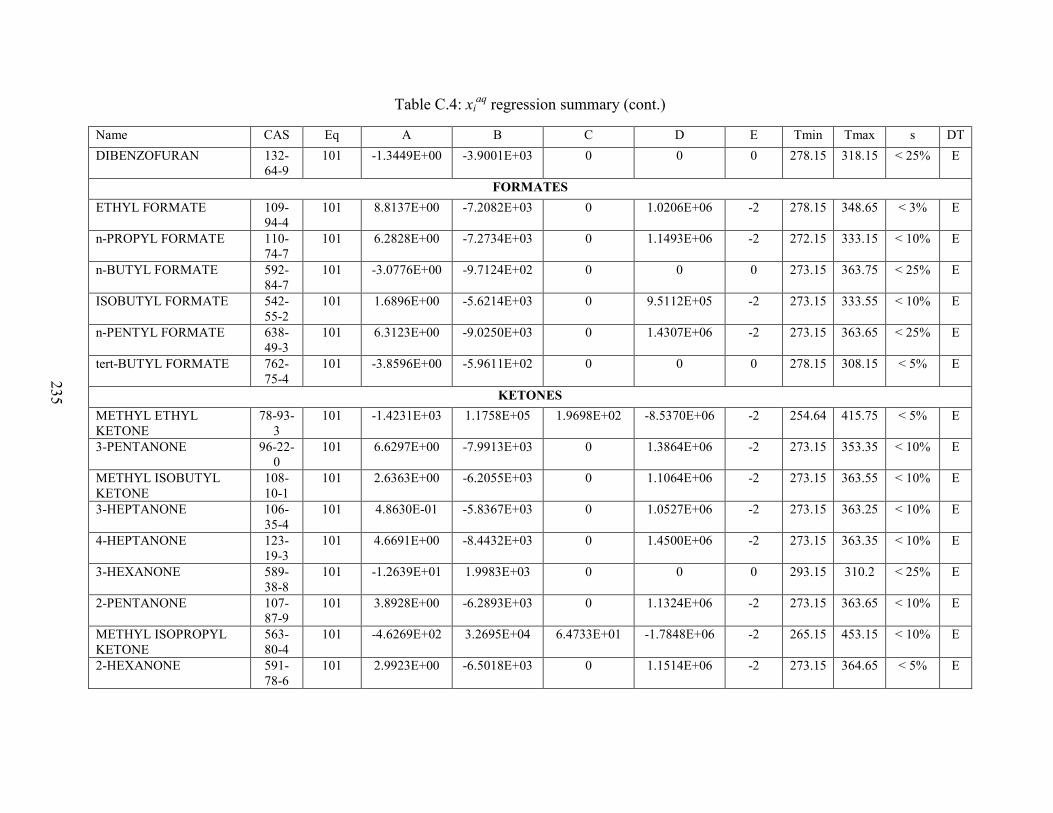
235

Table C.4: xiaq regression summary (cont.)

Name CAS Eq A B C D E Tmin Tmax s DT DIBENZOFURAN 132-

64-9 101 -1.3449E+00 -3.9001E+03 0 0 0 278.15 318.15 < 25% E

FORMATES ETHYL FORMATE 109-

94-4 101 8.8137E+00 -7.2082E+03 0 1.0206E+06 -2 278.15 348.65 < 3% E

n-PROPYL FORMATE 110-74-7

101 6.2828E+00 -7.2734E+03 0 1.1493E+06 -2 272.15 333.15 < 10% E

n-BUTYL FORMATE 592-84-7

101 -3.0776E+00 -9.7124E+02 0 0 0 273.15 363.75 < 25% E

ISOBUTYL FORMATE 542-55-2

101 1.6896E+00 -5.6214E+03 0 9.5112E+05 -2 273.15 333.55 < 10% E

n-PENTYL FORMATE 638-49-3

101 6.3123E+00 -9.0250E+03 0 1.4307E+06 -2 273.15 363.65 < 25% E

tert-BUTYL FORMATE 762-75-4

101 -3.8596E+00 -5.9611E+02 0 0 0 278.15 308.15 < 5% E

KETONES METHYL ETHYL KETONE

78-93-3

101 -1.4231E+03 1.1758E+05 1.9698E+02 -8.5370E+06 -2 254.64 415.75 < 5% E

3-PENTANONE 96-22-0

101 6.6297E+00 -7.9913E+03 0 1.3864E+06 -2 273.15 353.35 < 10% E

METHYL ISOBUTYL KETONE

108-10-1

101 2.6363E+00 -6.2055E+03 0 1.1064E+06 -2 273.15 363.55 < 10% E

3-HEPTANONE 106-35-4

101 4.8630E-01 -5.8367E+03 0 1.0527E+06 -2 273.15 363.25 < 10% E

4-HEPTANONE 123-19-3

101 4.6691E+00 -8.4432E+03 0 1.4500E+06 -2 273.15 363.35 < 10% E

3-HEXANONE 589-38-8

101 -1.2639E+01 1.9983E+03 0 0 0 293.15 310.2 < 25% E

2-PENTANONE 107-87-9

101 3.8928E+00 -6.2893E+03 0 1.1324E+06 -2 273.15 363.65 < 10% E

METHYL ISOPROPYL KETONE

563-80-4

101 -4.6269E+02 3.2695E+04 6.4733E+01 -1.7848E+06 -2 265.15 453.15 < 10% E

2-HEXANONE 591-78-6

101 2.9923E+00 -6.5018E+03 0 1.1514E+06 -2 273.15 364.65 < 5% E

236

Table C.4: xiaq regression summary (cont.)

Name CAS Eq A B C D E Tmin Tmax s DT 2-HEPTANONE 110-

43-0 101 6.4375E+00 -9.3023E+03 0 1.5481E+06 -2 273.15 363.65 < 5% E

5-METHYL-2-HEXANONE

110-12-3

101 7.1688E+00 -9.6863E+03 0 1.6139E+06 -2 273.15 362.85 < 5% E

3,3-DIMETHYL-2-BUTANONE

75-97-8

101 -8.1543E-01 -4.0863E+03 0 7.8661E+05 -2 273.15 363.35 < 5% E

DIISOBUTYL KETONE 108-83-8

101 7.1063E+00 -1.1438E+04 0 1.9006E+06 -2 273.15 363.85 < 10% E

DIISOPROPYL KETONE 565-80-0

101 -2.1253E+00 -4.1921E+03 0 8.0333E+05 -2 273.15 363.45 < 10% E

5-NONANONE 502-56-7

101 1.7303E+00 -8.2199E+03 0 1.4280E+06 -2 273.15 363.75 < 25% E

2-NONANONE 821-55-6

101 5.8740E+00 -1.0490E+04 0 1.7112E+06 -2 273.15 364.35 < 25% E

ACETYLACETONE 123-54-6

101 1.6717E+01 -1.1122E+04 0 1.5290E+06 -2 273.15 363.65 < 10% E

ISOPHORONE 78-59-1

101 9.5687E+00 -1.0617E+04 0 1.7565E+06 -2 273.15 364.25 < 5% E

CYCLOPENTANONE 120-92-3

6000 -1.6081E+01 3.1202E+03 1.6210E-02 -2.9219E+00 378.15 267.45 378.15 < 3% E

CYCLOHEXANONE 108-94-1

101 6.6031E+00 -7.5035E+03 0 1.2904E+06 -2 273.15 363.85 < 5% E

2-OCTANONE 111-13-7

101 7.7020E+00 -1.1250E+04 0 1.9033E+06 -2 273.15 364.15 < 25% E

ACETOPHENONE 98-86-2

101 2.1398E+00 -4.5194E+03 0 5.3558E+05 -2 293.05 353.35 < 25% E

3-OCTANONE 106-68-3

101 -1.6485E+00 -5.0117E+03 0 8.7634E+05 -2 273.15 364.15 < 10% E

3-NONANONE 925-78-0

101 -9.4462E+00 -6.6198E+01 0 0 0 273.15 353.35 < 25% E

2,6,8-TRIMETHYL-4-NONANONE

123-18-2

100 2.2065E-06 0 0 0 0 298.15 298.15 < 25% P

237

Table C.4: xiaq regression summary (cont.)

Name CAS Eq A B C D E Tmin Tmax s DT MERCAPTANS

ISOPROPYL MERCAPTAN

75-33-2

101 -7.3515E+00 9.3654E+01 0 0 0 288.15 318.15 < 10% E

n-BUTYL MERCAPTAN 109-79-5

101 1.8888E+01 -1.6328E+04 0 2.4137E+06 -2 288.15 333.15 < 5% E

METHYLALKANES 2-METHYLPENTANE 107-

83-5 101 1.6772E+01 -1.8364E+04 0 2.8566E+06 -2 273.15 422.65 < 25% E

3-METHYLPENTANE 96-14-0

100 2.7067E-06 0 0 0 0 298.15 298.15 < 3% S

2-METHYLHEXANE 591-76-4

100 4.5667E-07 0 0 0 0 298.15 298.15 < 5% E

3-METHYLHEXANE 589-34-4

100 4.7716E-07 0 0 0 0 298.15 298.15 < 5% E

3-METHYLHEPTANE 589-81-1

100 1.2491E-07 0 0 0 0 298.15 298.15 < 5% E

4-METHYLHEPTANE 589-53-7

100 1.3224E-07 0 0 0 0 298.15 298.15 < 5% E

N-ALCOHOLS 1-BUTANOL 71-36-

3 6000 -1.6135E+01 3.2105E+03 1.5570E-02 -5.1405E+00 398.31 273.15 398.3 < 3% E

1-PENTANOL 71-41-0

101 7.8962E+00 -8.7669E+03 0 1.4281E+06 -2 273.15 368.95 < 3% E

1-HEXANOL 111-27-3

101 8.2658E+00 -9.8737E+03 0 1.5999E+06 -2 273.15 363.45 < 10% E

1-HEPTANOL 111-70-6

101 1.8876E+01 -1.7053E+04 0 2.6686E+06 -2 273.15 363.65 < 10% E

1-OCTANOL 111-87-5

101 1.8301E+01 -1.7025E+04 0 2.5985E+06 -2 288.15 363.45 < 10% EP

1-NONANOL 143-08-8

101 1.8177E+01 -1.7366E+04 0 2.5783E+06 -2 288.15 363.15 < 25% E

1-DECANOL 112-30-1

101 2.2457E+01 -2.0308E+04 0 2.9573E+06 -2 288.15 363.15 < 10% E

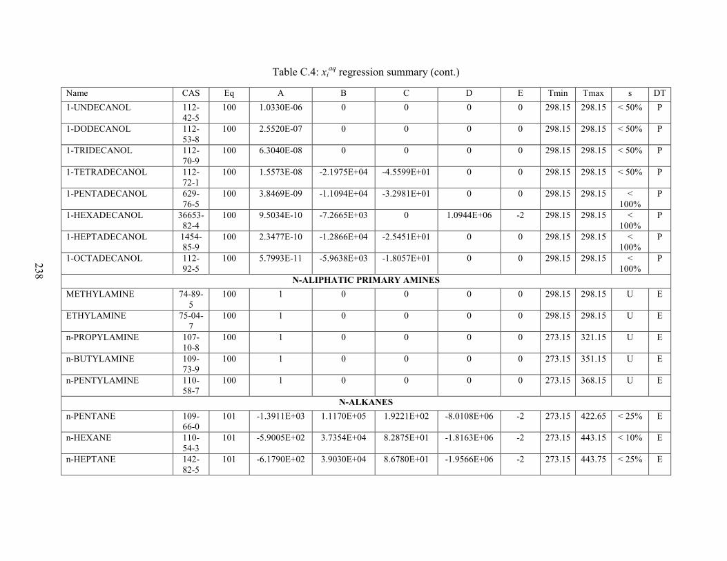
238

Table C.4: xiaq regression summary (cont.)

Name CAS Eq A B C D E Tmin Tmax s DT 1-UNDECANOL 112-

42-5 100 1.0330E-06 0 0 0 0 298.15 298.15 < 50% P

1-DODECANOL 112-53-8

100 2.5520E-07 0 0 0 0 298.15 298.15 < 50% P

1-TRIDECANOL 112-70-9

100 6.3040E-08 0 0 0 0 298.15 298.15 < 50% P

1-TETRADECANOL 112-72-1

100 1.5573E-08 -2.1975E+04 -4.5599E+01 0 0 298.15 298.15 < 50% P

1-PENTADECANOL 629-76-5

100 3.8469E-09 -1.1094E+04 -3.2981E+01 0 0 298.15 298.15 < 100%

P

1-HEXADECANOL 36653-82-4

100 9.5034E-10 -7.2665E+03 0 1.0944E+06 -2 298.15 298.15 < 100%

P

1-HEPTADECANOL 1454-85-9

100 2.3477E-10 -1.2866E+04 -2.5451E+01 0 0 298.15 298.15 < 100%

P

1-OCTADECANOL 112-92-5

100 5.7993E-11 -5.9638E+03 -1.8057E+01 0 0 298.15 298.15 < 100%

P

N-ALIPHATIC PRIMARY AMINES METHYLAMINE 74-89-

5 100 1 0 0 0 0 298.15 298.15 U E

ETHYLAMINE 75-04-7

100 1 0 0 0 0 298.15 298.15 U E

n-PROPYLAMINE 107-10-8

100 1 0 0 0 0 273.15 321.15 U E

n-BUTYLAMINE 109-73-9

100 1 0 0 0 0 273.15 351.15 U E

n-PENTYLAMINE 110-58-7

100 1 0 0 0 0 273.15 368.15 U E

N-ALKANES n-PENTANE 109-

66-0 101 -1.3911E+03 1.1170E+05 1.9221E+02 -8.0108E+06 -2 273.15 422.65 < 25% E

n-HEXANE 110-54-3

101 -5.9005E+02 3.7354E+04 8.2875E+01 -1.8163E+06 -2 273.15 443.15 < 10% E

n-HEPTANE 142-82-5

101 -6.1790E+02 3.9030E+04 8.6780E+01 -1.9566E+06 -2 273.15 443.75 < 25% E

239

Table C.4: xiaq regression summary (cont.)

Name CAS Eq A B C D E Tmin Tmax s DT n-OCTANE 111-

65-9 101 2.6143E+01 -2.5670E+04 0 3.9079E+06 -2 273.15 456.15 < 25% E

n-NONANE 111-84-2

101 4.0403E+01 -3.6046E+04 0 5.5730E+06 -2 287.95 409.75 < 50% E

n-DECANE 124-18-5

100 4.3460E-09 0 0 0 0 298.15 298.15 < 50% S

N-ALKYLBENZENES BENZENE 71-43-

2 101 8.8569E+00 -9.5142E+03 0 1.3553E+06 -2 273.15 527.15 < 3% E

TOLUENE 108-88-3

101 8.9793E+00 -1.0140E+04 0 1.4189E+06 -2 261.7 473.55 < 5% E

ETHYLBENZENE 100-41-4

101 1.4054E+01 -1.4454E+04 0 2.1340E+06 -2 273.15 373.15 < 5% E

n-PROPYLBENZENE 103-65-1

101 4.5679E+00 -8.9194E+03 0 1.2076E+06 -2 273.65 328.15 < 10% E

n-BUTYLBENZENE 104-51-8

101 1.7850E+01 -1.7506E+04 0 2.4576E+06 -2 273.65 373.15 < 5% E

n-HEPTYLBENZENE 1078-71-3

100 2.3098E-08 -1.0897E+04 -3.2652E+01 0 0 298.15 298.15 < 5% P

n-DECYLBENZENE 104-72-3

100 2.0688E-10 -9.7708E+03 -4.2873E+01 3.6254E-02 1 298.15 298.15 < 10% S

n-PENTYLBENZENE 538-68-1

101 1.1262E+01 -1.4633E+04 0 2.0603E+06 -2 280.15 318.15 < 10% E

n-HEXYLBENZENE 1077-16-3

101 6.7333E+00 -1.2793E+04 0 1.7900E+06 -2 278.15 318.15 < 3% E

n-OCTYLBENZENE 2189-60-8

100 4.9663E-09 0 0 0 0 298.15 298.15 < 10% P

n-NONYLBENZENE 1081-77-2

100 1.0313E-09 0 0 0 0 298.15 298.15 < 10% P

NAPHTHALENES NAPHTHALENE 91-20-

3 101 2.0659E+01 -1.6308E+04 0 1.9288E+06 -2 275.05 346.55 < 3% E

1-METHYL-NAPHTHALENE

90-12-0

101 -8.4391E+00 -1.2142E+03 0 0 0 277.25 304.85 < 10% E

240

Table C.4: xiaq regression summary (cont.)

Name CAS Eq A B C D E Tmin Tmax s DT 2-METHYL-NAPHTHALENE

91-57-6

101 -2.6452E+00 -3.0013E+03 0 0 0 277.25 304.15 < 25% E

1-ETHYL-NAPHTHALENE

1127-76-0

101 -7.4377E+00 -1.8483E+03 0 0 0 281.55 304.85 < 10% E

NITRILES PROPIONITRILE 107-

12-0 101 1.5998E+01 -1.1438E+04 0 1.6904E+06 -2 298.15 353.15 < 5% E

ACRYLONITRILE 107-13-1

101 5.6317E+00 -5.4279E+03 0 7.8429E+05 -2 273.15 343.15 < 5% E

METHACRYLO-NITRILE

126-98-7

101 1.2848E+01 -1.0849E+04 0 1.6366E+06 -2 273.15 353.15 < 10% E

SUCCINONITRILE 110-61-2

6000 1.4744E+02 -2.4452E+04 -2.2705E-01 -3.3471E+00 329.01 305 329 < 3% E

GLUTARONITRILE 544-13-8

5000 -1.3892E+04 8.9362E+04 2.0360E+03 1.7487E+03 342.00 290 342 < 10% E

n-BUTYRONITRILE 109-74-0

101 1.1169E+00 -3.7470E+03 0 5.9779E+05 -2 273.15 363.15 < 3% E

VALERONITRILE 110-59-8

101 1.5015E+01 -1.2632E+04 0 1.9077E+06 -2 273.15 363.15 < 10% E

ISOBUTYRO-NITRILE 78-82-0

101 -4.5050E-01 -2.6707E+03 0 4.2005E+05 -2 273.15 363.15 < 5% E

BENZONITRILE 100-47-0

101 -3.8294E+00 -1.0182E+03 0 0 0 273.15 363.15 < 25% E

VINYL-ACETONITRILE 109-75-1

101 9.3859E+00 -8.2424E+03 0 1.2031E+06 -2 273.15 363.15 < 5% E

PHENYL-ACETONITRILE

140-29-4

101 1.5843E+01 -1.3292E+04 0 1.8234E+06 -2 273.15 363.15 < 25% E

NITROAMINES o-NITROANILINE 88-74-

4 101 7.2633E+00 -4.8220E+03 0 0 0 298.15 313.25 < 50% E

p-NITROANILINE 100-01-6

101 7.2258E+00 -4.9899E+03 0 0 0 293.15 313.25 < 10% E

m-NITROANILINE 99-09-2

6000 2.2651E+00 -3.5004E+03 5.9660E-03 -1.8641E+00 458.36 273.15 458.35 < 10% E

241

Table C.4: xiaq regression summary (cont.)

Name CAS Eq A B C D E Tmin Tmax s DT ORGANIC SALTS

DIETHYL CARBONATE 105-58-8

101 6.3888E+00 -8.1262E+03 0 1.3289E+06 -2 273.15 363.45 < 5% E

DIMETHYL CARBONATE

616-38-6

101 4.6151E+00 -4.7448E+03 0 6.8616E+05 -2 282.95 333.55 < 3% E

OTHER ALIPHATIC ALCOHOLS 2-METHYL-1-PROPANOL

78-83-1

101 -2.3310E+03 1.9509E+05 3.2240E+02 -1.4587E+07 -2 273.15 407.25 < 10% E

2-BUTANOL 78-92-2

6000 -2.3732E+01 4.4883E+03 2.6387E-02 -3.5525E+00 386.65 273.15 386.65 < 3% E

2-PENTANOL 6032-29-7

101 6.9003E+00 -8.2230E+03 0 1.4184E+06 -2 273.15 363.45 < 5% E

2-METHYL-2-BUTANOL 75-85-4

101 -1.8723E+03 1.5768E+05 2.5837E+02 -1.1765E+07 -2 273.65 401.75 < 10% E

2-METHYL-1-BUTANOL 137-32-6

101 8.0268E+00 -8.9236E+03 0 1.4838E+06 -2 273.65 363.95 < 5% E

2,2-DIMETHYL-1-PROPANOL

75-84-3

101 4.5624E+00 -6.9514E+03 0 1.2234E+06 -2 285.15 363.15 < 10% E

2-HEXANOL 626-93-7

101 7.9408E+00 -9.6532E+03 0 1.6249E+06 -2 273.15 363.35 < 10% E

3-HEXANOL 623-37-0

101 6.2630E+00 -8.7820E+03 0 1.5363E+06 -2 273.15 363.45 < 5% E

3-METHYL-1-PENTANOL

589-35-5

101 1.0298E+01 -1.0896E+04 0 1.7641E+06 -2 273.15 363.65 < 5% E

3-METHYL-3-PENTANOL

77-74-7

101 -9.2854E+00 1.2486E+03 0 0 0 282.95 363.55 < 10% E

3-PENTANOL 584-02-1

101 7.0880E+00 -8.4508E+03 0 1.4859E+06 -2 273.15 363.15 < 5% E

3-METHYL-1-BUTANOL 123-51-3

101 5.1443E+00 -7.1281E+03 0 1.2022E+06 -2 273.15 363.15 < 5% E

3-METHYL-2-BUTANOL 598-75-4

101 -1.3435E+03 1.1083E+05 1.8565E+02 -8.0438E+06 -2 273.15 363.15 < 5% E

2-HEPTANOL 543-49-7

101 8.9387E+00 -1.1008E+04 0 1.8246E+06 -2 273.15 363.35 < 10% E

242

Table C.4: xiaq regression summary (cont.)

Name CAS Eq A B C D E Tmin Tmax s DT 3-HEPTANOL 589-

82-2 101 5.5168E+00 -9.1575E+03 0 1.5956E+06 -2 273.15 363.35 < 10% E

4-METHYL-2-PENTANOL

108-11-2

101 5.0667E+00 -7.8098E+03 0 1.3557E+06 -2 273.15 363.35 < 10% E

2-OCTANOL 123-96-6

101 1.6068E+01 -1.6328E+04 0 2.6604E+06 -2 273.15 363.65 < 10% E

2-NONANOL 628-99-9

101 1.3272E+01 -1.5882E+04 0 2.6529E+06 -2 273.15 363.65 < 25% E

2,6-DIMETHYL-4-HEPTANOL

108-82-7

101 -3.2973E+00 -5.3209E+03 0 1.0358E+06 -2 273.15 363.65 < 25% E

OTHER ALIPHATIC AMINES TRIETHYLAMINE 121-

44-8 6000 2.7364E+01 -5.2885E+03 -3.9158E-02 -7.5913E+00 291.14 291.15 353.15 < 25% E

DI-n-PROPYLAMINE 142-84-7

6000 1.1999E+01 -2.2185E+03 -2.2788E-02 -5.6220E+00 268.34 268.35 363.15 < 25% E

N,N-DIMETHYL-n-BUTYLAMINE

927-62-8

6000 -2.4897E+01 4.2843E+03 1.9112E-02 -1.2491E+00 276.94 276.95 363.15 < 25% E

N,N-DIETHYL-METHYLAMINE

616-39-7

6000 3.7296E+02 -6.6421E+04 -5.2238E-01 -1.0773E+01 322.05 322.06 351.43 < 25% E

DIETHYLAMINE 109-89-7

100 1 0 0 0 0 273.15 328.15 U E

DIISOPROPYLAMINE 108-18-9

6000 1.2988E+02 -2.2447E+04 -1.9105E-01 -8.2043E+00 300.17 300.18 357.15 < 25% E

DI-n-BUTYLAMINE 111-92-2

101 4.2595E+00 -9.3265E+03 0 1.7549E+06 -2 273.15 363.15 < 10% E

TRI-n-BUTYLAMINE 102-82-9

101 -1.3391E+01 1.1860E+03 0 0 0 273.15 353.15 < 25% E

OTHER ALKANES 2,3,4-TRIMETHYL-PENTANE

565-75-3

100 2.1260E-07 1.1974E+04 3.1657E+01 0 0 298.15 298.15 < 5% S

2,2,5-TRIMETHYL-HEXANE

3522-94-9

101 -2.0551E+01 1.2394E+03 0 0 0 273.15 298.15 < 5% E

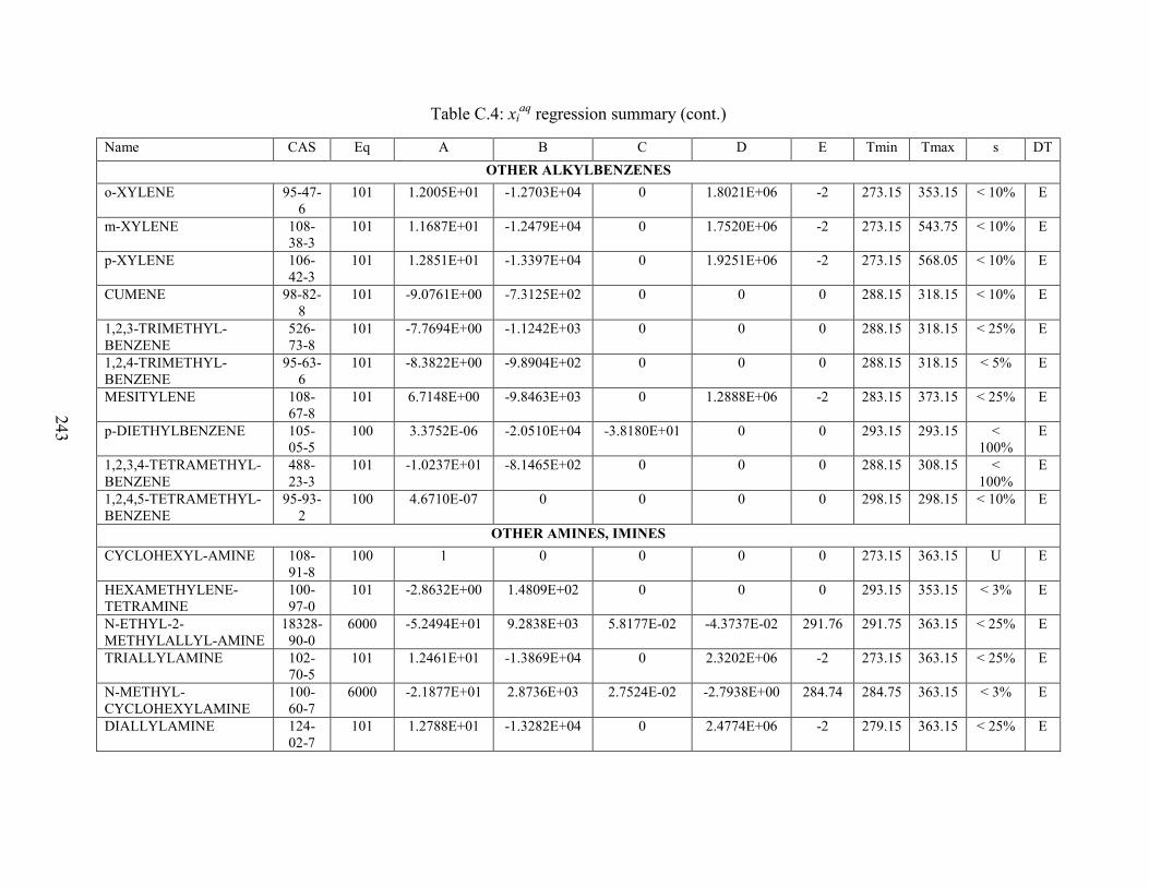
243

Table C.4: xiaq regression summary (cont.)

Name CAS Eq A B C D E Tmin Tmax s DT OTHER ALKYLBENZENES

o-XYLENE 95-47-6

101 1.2005E+01 -1.2703E+04 0 1.8021E+06 -2 273.15 353.15 < 10% E

m-XYLENE 108-38-3

101 1.1687E+01 -1.2479E+04 0 1.7520E+06 -2 273.15 543.75 < 10% E

p-XYLENE 106-42-3

101 1.2851E+01 -1.3397E+04 0 1.9251E+06 -2 273.15 568.05 < 10% E

CUMENE 98-82-8

101 -9.0761E+00 -7.3125E+02 0 0 0 288.15 318.15 < 10% E

1,2,3-TRIMETHYL-BENZENE

526-73-8

101 -7.7694E+00 -1.1242E+03 0 0 0 288.15 318.15 < 25% E

1,2,4-TRIMETHYL-BENZENE

95-63-6

101 -8.3822E+00 -9.8904E+02 0 0 0 288.15 318.15 < 5% E

MESITYLENE 108-67-8

101 6.7148E+00 -9.8463E+03 0 1.2888E+06 -2 283.15 373.15 < 25% E

p-DIETHYLBENZENE 105-05-5

100 3.3752E-06 -2.0510E+04 -3.8180E+01 0 0 293.15 293.15 < 100%

E

1,2,3,4-TETRAMETHYL-BENZENE

488-23-3

101 -1.0237E+01 -8.1465E+02 0 0 0 288.15 308.15 < 100%

E

1,2,4,5-TETRAMETHYL-BENZENE

95-93-2

100 4.6710E-07 0 0 0 0 298.15 298.15 < 10% E

OTHER AMINES, IMINES CYCLOHEXYL-AMINE 108-

91-8 100 1 0 0 0 0 273.15 363.15 U E

HEXAMETHYLENE-TETRAMINE

100-97-0

101 -2.8632E+00 1.4809E+02 0 0 0 293.15 353.15 < 3% E

N-ETHYL-2-METHYLALLYL-AMINE

18328-90-0

6000 -5.2494E+01 9.2838E+03 5.8177E-02 -4.3737E-02 291.76 291.75 363.15 < 25% E

TRIALLYLAMINE 102-70-5

101 1.2461E+01 -1.3869E+04 0 2.3202E+06 -2 273.15 363.15 < 25% E

N-METHYL-CYCLOHEXYLAMINE

100-60-7

6000 -2.1877E+01 2.8736E+03 2.7524E-02 -2.7938E+00 284.74 284.75 363.15 < 3% E

DIALLYLAMINE 124-02-7

101 1.2788E+01 -1.3282E+04 0 2.4774E+06 -2 279.15 363.15 < 25% E

244

Table C.4: xiaq regression summary (cont.)

Name CAS Eq A B C D E Tmin Tmax s DT N-METHYLPIPERIDINE 626-

67-5 6000 -2.6040E+01 3.9739E+03 3.2166E-02 -3.2579E+00 317.14 317.15 363.15 < 10% E

OTHER CONDENSED RINGS FLUORANTHENE 206-

44-0 101 3.6246E-01 -5.3775E+03 0 0 0 281.25 333.15 < 10% E

FLUORENE 86-73-7

101 -4.1946E-01 -4.4885E+03 0 0 0 279.75 333.15 < 10% E

ANTHRACENE 120-12-7

101 2.3500E+01 -1.9563E+04 0 2.0384E+06 -2 273.45 347.85 < 5% E

PHENANTHRENE 85-01-8

101 1.9291E+01 -1.6237E+04 0 1.6996E+06 -2 277.15 346.55 < 5% E

CHRYSENE 218-01-9

101 -8.7436E+00 -4.1710E+03 0 0 0 279.65 302.15 < 25% E

PYRENE 129-00-0

101 2.0676E+01 -1.8288E+04 0 1.9905E+06 -2 277.85 347.85 < 5% E

ACENAPHTHENE 83-32-9

101 2.2202E+00 -5.0460E+03 0 0 0 277.25 347.85 < 25% E

ACENAPHTHALENE 208-96-8

101 -4.9130E+00 -2.5248E+03 0 0 0 277.25 304.15 < 25% E

BENZO[a]PYRENE 50-32-8

101 -6.0895E+00 -5.0166E+03 0 0 0 281.15 308.15 < 10% E

BENZANTHRACENE 56-55-3

101 1.1722E+02 -7.6026E+04 0 1.0373E+07 -2 276.85 308.15 < 10% E

BENZO[b]FLUOR-ANTHENE

205-99-2

101 6.9573E+00 -8.9149E+03 0 0 0 283.15 328.15 < 10% E

OTHER ETHERS/DIETHERS METHYLAL 109-

87-5 101 -3.7046E+00 3.8855E+02 0 0 0 273.15 313.15 < 10% E

1,2-DIMETHOXYETHANE

110-71-4

101 -5.6795E+00 8.8936E+02 0 0 0 273.15 313.15 < 25% E

DIETHYLENE GLYCOL DIETHYL ETHER

112-36-7

6000 -6.1762E+01 1.1670E+04 6.9790E-02 4.4908E-02 301.14 301.15 363.25 < 10% E

DIETHYLENE GLYCOL DI-n-BUTYL ETHER

112-73-2

101 1.4893E+01 -1.7993E+04 0 3.2683E+06 -2 273.15 363.15 < 10% E

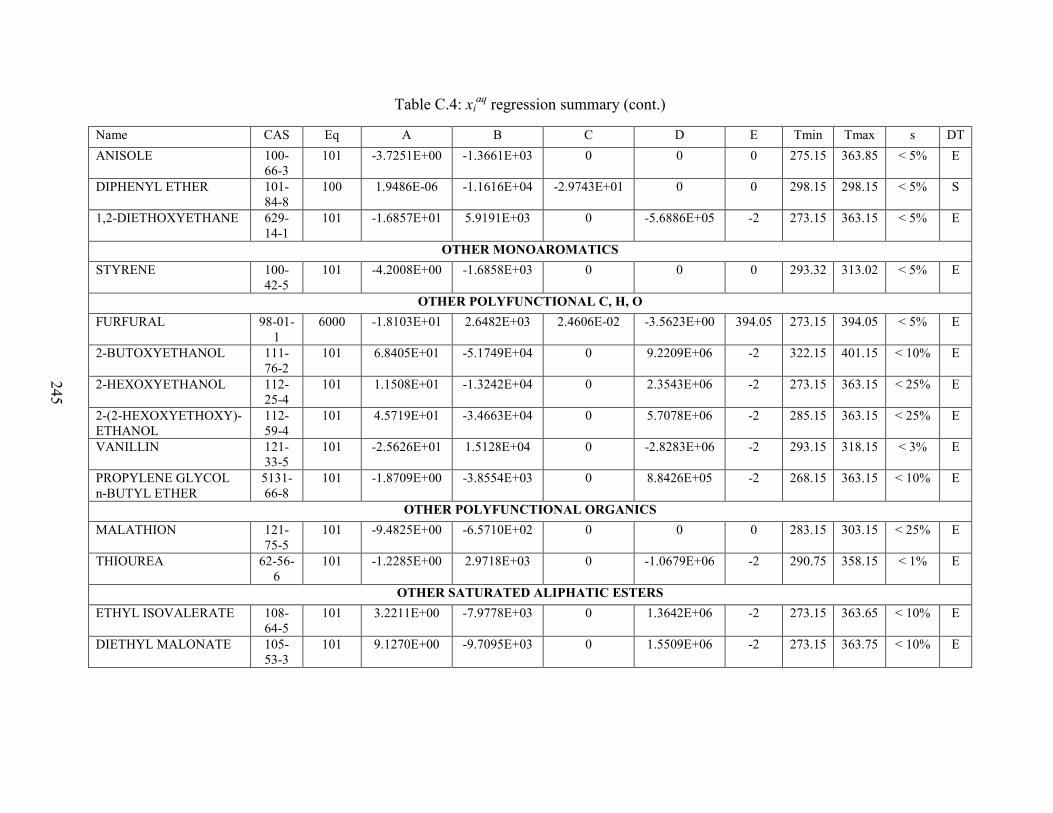
245

Table C.4: xiaq regression summary (cont.)

Name CAS Eq A B C D E Tmin Tmax s DT ANISOLE 100-

66-3 101 -3.7251E+00 -1.3661E+03 0 0 0 275.15 363.85 < 5% E

DIPHENYL ETHER 101-84-8

100 1.9486E-06 -1.1616E+04 -2.9743E+01 0 0 298.15 298.15 < 5% S

1,2-DIETHOXYETHANE 629-14-1

101 -1.6857E+01 5.9191E+03 0 -5.6886E+05 -2 273.15 363.15 < 5% E

OTHER MONOAROMATICS STYRENE 100-

42-5 101 -4.2008E+00 -1.6858E+03 0 0 0 293.32 313.02 < 5% E

OTHER POLYFUNCTIONAL C, H, O FURFURAL 98-01-

1 6000 -1.8103E+01 2.6482E+03 2.4606E-02 -3.5623E+00 394.05 273.15 394.05 < 5% E

2-BUTOXYETHANOL 111-76-2

101 6.8405E+01 -5.1749E+04 0 9.2209E+06 -2 322.15 401.15 < 10% E

2-HEXOXYETHANOL 112-25-4

101 1.1508E+01 -1.3242E+04 0 2.3543E+06 -2 273.15 363.15 < 25% E

2-(2-HEXOXYETHOXY)-ETHANOL

112-59-4

101 4.5719E+01 -3.4663E+04 0 5.7078E+06 -2 285.15 363.15 < 25% E

VANILLIN 121-33-5

101 -2.5626E+01 1.5128E+04 0 -2.8283E+06 -2 293.15 318.15 < 3% E

PROPYLENE GLYCOL n-BUTYL ETHER

5131-66-8

101 -1.8709E+00 -3.8554E+03 0 8.8426E+05 -2 268.15 363.15 < 10% E

OTHER POLYFUNCTIONAL ORGANICS MALATHION 121-

75-5 101 -9.4825E+00 -6.5710E+02 0 0 0 283.15 303.15 < 25% E

THIOUREA 62-56-6

101 -1.2285E+00 2.9718E+03 0 -1.0679E+06 -2 290.75 358.15 < 1% E

OTHER SATURATED ALIPHATIC ESTERS ETHYL ISOVALERATE 108-

64-5 101 3.2211E+00 -7.9778E+03 0 1.3642E+06 -2 273.15 363.65 < 10% E

DIETHYL MALONATE 105-53-3

101 9.1270E+00 -9.7095E+03 0 1.5509E+06 -2 273.15 363.75 < 10% E

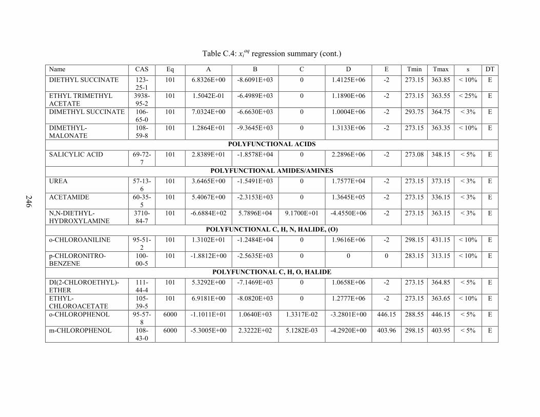
246

Table C.4: xiaq regression summary (cont.)

Name CAS Eq A B C D E Tmin Tmax s DT DIETHYL SUCCINATE 123-

25-1 101 6.8326E+00 -8.6091E+03 0 1.4125E+06 -2 273.15 363.85 < 10% E

ETHYL TRIMETHYL ACETATE

3938-95-2

101 1.5042E-01 -6.4989E+03 0 1.1890E+06 -2 273.15 363.55 < 25% E

DIMETHYL SUCCINATE 106-65-0

101 7.0324E+00 -6.6630E+03 0 1.0004E+06 -2 293.75 364.75 < 3% E

DIMETHYL-MALONATE

108-59-8

101 1.2864E+01 -9.3645E+03 0 1.3133E+06 -2 273.15 363.35 < 10% E

POLYFUNCTIONAL ACIDS SALICYLIC ACID 69-72-

7 101 2.8389E+01 -1.8578E+04 0 2.2896E+06 -2 273.08 348.15 < 5% E

POLYFUNCTIONAL AMIDES/AMINES UREA 57-13-

6 101 3.6465E+00 -1.5491E+03 0 1.7577E+04 -2 273.15 373.15 < 3% E

ACETAMIDE 60-35-5

101 5.4067E+00 -2.3153E+03 0 1.3645E+05 -2 273.15 336.15 < 3% E

N,N-DIETHYL-HYDROXYLAMINE

3710-84-7

101 -6.6884E+02 5.7896E+04 9.1700E+01 -4.4550E+06 -2 273.15 363.15 < 3% E

POLYFUNCTIONAL C, H, N, HALIDE, (O) o-CHLOROANILINE 95-51-

2 101 1.3102E+01 -1.2484E+04 0 1.9616E+06 -2 298.15 431.15 < 10% E

p-CHLORONITRO-BENZENE

100-00-5

101 -1.8812E+00 -2.5635E+03 0 0 0 283.15 313.15 < 10% E

POLYFUNCTIONAL C, H, O, HALIDE DI(2-CHLOROETHYL)-ETHER

111-44-4

101 5.3292E+00 -7.1469E+03 0 1.0658E+06 -2 273.15 364.85 < 5% E

ETHYL-CHLOROACETATE

105-39-5

101 6.9181E+00 -8.0820E+03 0 1.2777E+06 -2 273.15 363.65 < 10% E

o-CHLOROPHENOL 95-57-8

6000 -1.1011E+01 1.0640E+03 1.3317E-02 -3.2801E+00 446.15 288.55 446.15 < 5% E

m-CHLOROPHENOL 108-43-0

6000 -5.3005E+00 2.3222E+02 5.1282E-03 -4.2920E+00 403.96 298.15 403.95 < 5% E

247

Table C.4: xiaq regression summary (cont.)

Name CAS Eq A B C D E Tmin Tmax s DT p-CHLOROPHENOL 106-

48-9 6000 -1.6519E+01 2.3389E+03 2.0971E-02 -5.1532E+00 402.41 272.95 402.4 < 25% E

METHYL CHLOROACETATE

96-34-4

101 5.2524E+00 -5.9225E+03 0 8.7840E+05 -2 273.15 363.25 < 5% E

POLYFUNCTIONAL C, H, O, N ACETAMINOPHEN 103-

90-2 101 3.0067E+01 -1.9166E+04 0 2.4749E+06 -2 278.15 343.15 < 5% E

ACETANILIDE 103-84-4

101 2.3705E+00 -2.8256E+03 0 0 0 293.15 303.15 < 25% E

POLYFUNCTIONAL ESTERS METHYL SALICYLATE 119-

36-8 101 6.3814E+00 -8.3884E+03 0 1.1532E+06 -2 273.15 363.65 < 25% E

2-ETHOXYETHYL ACETATE

111-15-9

101 -7.8319E+00 1.3675E+03 0 0 0 273.15 363.15 < 5% E

ETHYL ACETOACETATE

141-97-9

101 -6.1053E+00 5.8199E+02 0 0 0 273.15 303.15 < 25% E

ETHYLENE GLYCOL MONOBUTYL ETHER ACETATE

112-07-2

101 1.0526E+01 -1.1809E+04 0 2.0227E+06 -2 273.15 363.35 < 25% E

POLYOLS p-HYDROQUINONE 123-

31-9 101 3.4838E+01 -2.0077E+04 0 2.4975E+06 -2 280.5 342.1 < 3% E

XYLITOL 87-99-0

101 6.3503E+00 -2.4082E+03 0 0 0 293.28 328.21 < 5% E

1,3-BENZENEDIOL 108-46-3

101 5.3815E+00 -2.0610E+03 0 0 0 298.15 382.55 < 3% E

PROPIONATES AND BUTYRATES METHYL PROPIONATE 554-

12-1 101 -5.4523E-01 -3.0228E+03 0 5.6240E+05 -2 273.15 343.35 < 3% E

ETHYL PROPIONATE 105-37-3

101 8.6870E+00 -9.6576E+03 0 1.6020E+06 -2 273.15 353.45 < 25% E

n-PROPYL PROPIONATE

106-36-5

101 2.3221E+00 -6.9160E+03 0 1.2331E+06 -2 273.15 363.65 < 10% E

248

Table C.4: xiaq regression summary (cont.)

Name CAS Eq A B C D E Tmin Tmax s DT n-BUTYL PROPIONATE 590-

01-2 101 4.6182E+00 -8.9538E+03 0 1.5193E+06 -2 273.15 363.55 < 5% E

n-PROPYL n-BUTYRATE 105-66-8

101 4.9548E+00 -8.9029E+03 0 1.4776E+06 -2 273.15 363.65 < 25% E

METHYL n-BUTYRATE 623-42-7

101 2.4057E+00 -5.8594E+03 0 1.0181E+06 -2 273.15 363.65 < 25% E

ETHYL n-BUTYRATE 105-54-4

101 -1.0853E-01 -5.2994E+03 0 9.7757E+05 -2 273.15 363.65 < 25% E

ISOBUTYL ISOBUTYRATE

97-85-8

101 3.3149E+00 -8.8385E+03 0 1.4943E+06 -2 273.15 363.45 < 25% E

n-BUTYL n-BUTYRATE 109-21-7

101 8.5669E+00 -1.2335E+04 0 2.0772E+06 -2 273.15 363.45 < 10% E

METHYL ISOBUTYRATE

547-63-7

101 1.6346E+00 -5.4561E+03 0 9.7055E+05 -2 273.15 353.45 < 3% E

ETHYL ISOBUTYRATE 97-62-1

101 -2.9548E-01 -5.2398E+03 0 9.7076E+05 -2 273.15 363.75 < 10% E

n-PENTYL n-BUTYRATE 540-18-1

101 -1.1103E+01 2.1889E+02 0 0 0 273.15 363.65 < 25% E

ISOPENTYL BUTYRATE 106-27-4

101 4.3536E+00 -1.0210E+04 0 1.7238E+06 -2 282.55 363.85 < 100%

E

SULFIDES/THIOPHENES DIMETHYL SULFIDE 75-18-

3 101 6.9652E+00 -7.2665E+03 0 1.0944E+06 -2 272.35 353.45 < 25% EP

DIMETHYL DISULFIDE 624-92-0

101 -4.5077E+00 -8.8322E+02 0 0 0 273.2 343.15 < 10% P

2-METHYLTHIOPHENE 554-14-3

101 -7.2777E+00 -3.1058E+02 0 0 0 298.15 343.15 < 10% E

DIISOPROPYL SULFIDE 625-80-9

101 -1.2690E+01 2.1122E+03 0 -2.9537E+05 -2 298.15 343.15 < 25% E

UNSATURATED ALIPHATIC ESTERS ETHYL ACRYLATE 140-

88-5 101 1.0372E+00 -4.1664E+03 0 6.4977E+05 -2 298.6 360.2 < 10% E

METHYL METHACRYLATE

80-62-6

101 7.2435E+00 -8.2103E+03 0 1.2803E+06 -2 273.15 353.15 < 5% E

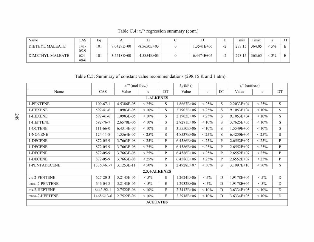
249

Table C.4: xiaq regression summary (cont.)

Name CAS Eq A B C D E Tmin Tmax s DT DIETHYL MALEATE 141-

05-9 101 7.0429E+00 -8.5650E+03 0 1.3541E+06 -2 273.15 364.05 < 5% E

DIMETHYL MALEATE 624-48-6

101 3.5518E+00 -4.5854E+03 0 6.4474E+05 -2 273.15 363.65 < 3% E

Table C.5: Summary of constant value recommendations (298.15 K and 1 atm) (cont.)

xiaq (mol frac.) kH (kPa) γi

∞ (unitless) Name CAS Value s DT Value s DT Value s DT

1-ALKENES 1-PENTENE 109-67-1 4.5386E-05 < 25% S 1.8667E+06 < 25% S 2.2033E+04 < 25% S 1-HEXENE 592-41-6 1.0983E-05 < 10% S 2.1902E+06 < 25% S 9.1053E+04 < 10% S 1-HEXENE 592-41-6 1.0983E-05 < 10% S 2.1902E+06 < 25% S 9.1053E+04 < 10% S 1-HEPTENE 592-76-7 2.6578E-06 < 10% S 2.8281E+06 < 10% S 3.7625E+05 < 10% S 1-OCTENE 111-66-0 6.4314E-07 < 10% S 3.5550E+06 < 10% S 1.5549E+06 < 10% S 1-NONENE 124-11-8 1.5564E-07 < 25% S 4.8537E+06 < 25% S 6.4250E+06 < 25% S 1-DECENE 872-05-9 3.7663E-08 < 25% P 6.4586E+06 < 25% P 2.6552E+07 < 25% P 1-DECENE 872-05-9 3.7663E-08 < 25% P 6.4586E+06 < 25% P 2.6552E+07 < 25% P 1-DECENE 872-05-9 3.7663E-08 < 25% P 6.4586E+06 < 25% P 2.6552E+07 < 25% P 1-DECENE 872-05-9 3.7663E-08 < 25% P 6.4586E+06 < 25% P 2.6552E+07 < 25% P 1-PENTADECENE 13360-61-7 3.1253E-11 < 50% S 2.4928E+07 < 50% S 3.1997E+10 < 50% S

2,3,4-ALKENES cis-2-PENTENE 627-20-3 5.2143E-05 < 5% E 1.2624E+06 < 5% D 1.9178E+04 < 5% D trans-2-PENTENE 646-04-8 5.2143E-05 < 5% E 1.2932E+06 < 5% D 1.9178E+04 < 5% D cis-2-HEPTENE 6443-92-1 2.7522E-06 < 10% E 2.3412E+06 < 10% D 3.6334E+05 < 10% D trans-2-HEPTENE 14686-13-6 2.7522E-06 < 10% E 2.2918E+06 < 10% D 3.6334E+05 < 10% D

ACETATES

250

Table C.5: Summary of constant value recommendations (298.15 K and 1 atm) (cont.)

xiaq (mol frac.) kH (kPa) γi

∞ (unitless) Name CAS Value s DT Value s DT Value s DT

METHYL ACETATE 79-20-9 6.9553E-02 < 3% S 6.7019E+02 < 10% S 2.3439E+01 < 10% S ETHYL ACETATE 141-78-6 1.6041E-02 < 3% S 8.4064E+02 < 10% S 6.7660E+01 < 10% S n-PROPYL ACETATE 109-60-4 3.7965E-03 < 5% S 1.2278E+03 < 10% S 2.7549E+02 < 10% S n-BUTYL ACETATE 123-86-4 1.0141E-03 < 10% S 1.4682E+03 < 10% S 9.8461E+02 < 10% S ISOBUTYL ACETATE 110-19-0 1.0669E-03 < 10% S 2.1658E+03 < 10% S 9.1034E+02 < 10% S ISOPENTYL ACETATE 123-92-2 2.9009E-04 < 10% S 2.7926E+03 < 10% S 3.4340E+03 < 10% S ISOPROPYL ACETATE 108-21-4 4.7173E-03 < 10% S 1.6585E+03 < 25% S 2.0593E+02 < 25% S sec-BUTYL ACETATE 105-46-4 1.2134E-03 < 10% S 2.4256E+03 < 10% S 8.1913E+02 < 10% S VINYL ACETATE 108-05-4 5.4579E-03 < 3% S 2.7687E+03 < 3% S 1.8316E+02 < 10% S n-PENTYL ACETATE 628-63-7 2.5034E-04 < 10% S 2.2402E+03 < 10% S 3.9828E+03 < 10% S n-HEXYL ACETATE 142-92-7 5.9728E-05 < 25% S 2.9135E+03 < 25% S 1.6595E+04 < 25% S n-HEPTYL ACETATE 112-06-1 1.5184E-05 < 25% P 3.8109E+03 < 25% P 6.5861E+04 < 25% P n-OCTYL ACETATE 112-14-1 3.7799E-06 < 25% P 5.4713E+03 < 25% P 2.6455E+05 < 25% P ETHYLENE GLYCOL DIACETATE

111-55-7 2.3492E-02 < 3% S - - - - - -

tert-BUTYL ACETATE 540-88-5 1.1407E-03 < 3% S 4.7259E+03 < 3% S 8.7411E+02 < 10% S CYCLOHEXYL ACETATE 622-45-7 3.4601E-04 < 10% S 5.0496E+02 < 10% S 2.8802E+03 < 25% S PHENYL ACETATE 122-79-2 7.6266E-04 < 5% S 4.2332E+01 < 5% S 1.3057E+03 < 25% S

ALDEHYDES ACETALDEHYDE 75-07-0 2.6796E-01 < 10% P 3.7813E+02 < 10% S - - - PROPANAL 123-38-6 1.2435E-01 < 25% S 4.3628E+02 < 5% S 1.0275E+01 < 5% S BUTANAL 123-72-8 1.7165E-02 < 10% S 6.0597E+02 < 5% S 4.0709E+01 < 10% S 2-METHYLPROPANAL 78-84-2 1.3236E-02 < 3% S 1.0934E+03 < 5% S 5.1912E+01 < 5% S PENTANAL 110-62-3 3.7043E-03 < 25% S 8.3509E+02 < 5% S 1.8344E+02 < 10% S HEPTANAL 111-71-7 2.3651E-04 < 10% S 1.6308E+03 < 10% S 3.1958E+03 < 25% S

251

Table C.5: Summary of constant value recommendations (298.15 K and 1 atm) (cont.)

xiaq (mol frac.) kH (kPa) γi

∞ (unitless) Name CAS Value s DT Value s DT Value s DT

HEXANAL 66-25-1 8.5071E-04 < 25% S 1.2229E+03 < 25% S 8.4624E+02 < 25% S OCTANAL 124-13-0 6.2433E-05 < 50% S 2.7045E+03 < 10% S 1.7662E+04 < 25% S NONANAL 124-19-6 7.2257E-06 < 50% S 4.9990E+03 < 25% S 1.3820E+05 < 25% S 2-ETHYLHEXANAL 123-05-7 5.6992E-05 < 25% S 4.7357E+03 < 25% S 1.7457E+04 < 25% S 2-ETHYL-2-HEXENAL 645-62-5 1.7449E-04 < 25% S 1.0617E+03 < 50% S 5.6988E+03 < 50% S DECANAL 112-31-2 1.4607E-06 < 50% S 8.7393E+03 < 100% S 6.8367E+05 < 100% S 2-METHYLBUTYRALDEHYDE 96-17-3 3.2304E-03 < 10% S 2.2328E+03 < 25% P 3.0863E+02 < 25% P ACROLEIN 107-02-8 8.6576E-02 < 10% S 7.6218E+02 < 100% E 2.0967E+01 > 100% S trans-CROTONALDEHYDE 123-73-9 4.6146E-02 < 10% S 1.0285E+02 < 25% S 2.1898E+01 < 25% S METHACROLEIN 78-85-3 1.6226E-02 < 10% S 1.2347E+03 < 10% S 6.1659E+01 < 10% S p-TOLUALDEHYDE 104-87-0 2.7792E-04 < 10% S 1.0440E+02 < 50% S 2.4875E+03 < 50% S BENZALDEHYDE 100-52-7 1.1842E-03 < 10% S 1.4523E+02 < 10% S 8.5631E+02 < 10% S m-TOLUALDEHYDE 620-23-5 - - - 1.6029E+02 < 25% S 3.5526E+03 < 50% S

ALIPHATIC ETHERS DIETHYL ETHER 60-29-7 1.5055E-02 < 3% S 5.7579E+03 < 3% S 8.0282E+01 < 5% S DIISOPROPYL ETHER 108-20-3 1.6091E-03 < 10% S 1.2343E+04 < 10% S 6.2256E+02 < 10% S DI-n-BUTYL ETHER 142-96-1 3.1637E-05 < 25% S 2.6272E+04 < 25% S 3.1840E+04 < 25% S METHYL tert-BUTYL ETHER 1634-04-4 8.0111E-03 < 5% S 4.1832E+03 < 5% S 1.2555E+02 < 10% S METHYL ISOBUTYL ETHER 625-44-5 2.2379E-03 < 5% S 1.2742E+04 < 10% S 4.4655E+02 < 10% S DI-n-HEXYL ETHER 112-58-3 6.8917E-08 < 25% P 8.9153E+04 < 25% P 1.4510E+07 < 25% P METHYL n-BUTYL ETHER 628-28-4 1.7201E-03 < 25% S 1.0077E+04 < 25% S 5.5095E+02 < 25% S DI-n-PENTYL ETHER 693-65-2 2.2173E-06 < 25% P 5.1508E+04 < 25% P 4.5100E+05 < 25% P METHYL tert-PENTYL ETHER 994-05-8 1.7852E-03 < 10% S 5.6708E+03 < 10% S 5.6458E+02 < 10% S tert-BUTYL ETHYL ETHER 637-92-3 2.6488E-03 < 25% S 7.7653E+03 < 10% S 4.6299E+02 < 25% S ETHYL tert-PENTYL ETHER 919-94-8 4.9313E-04 < 25% S 1.1017E+04 < 25% S 2.0257E+03 < 25% S

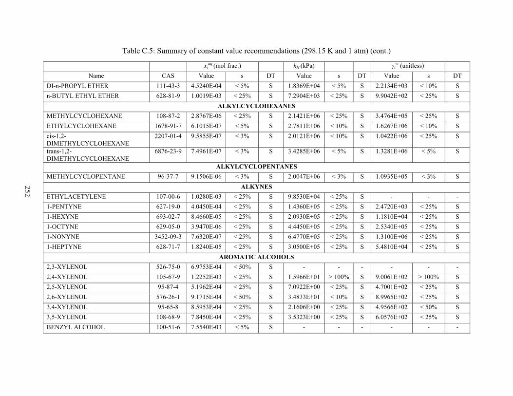
252

Table C.5: Summary of constant value recommendations (298.15 K and 1 atm) (cont.)

xiaq (mol frac.) kH (kPa) γi

∞ (unitless) Name CAS Value s DT Value s DT Value s DT

DI-n-PROPYL ETHER 111-43-3 4.5240E-04 < 5% S 1.8369E+04 < 5% S 2.2134E+03 < 10% S n-BUTYL ETHYL ETHER 628-81-9 1.0019E-03 < 25% S 7.2904E+03 < 25% S 9.9042E+02 < 25% S

ALKYLCYCLOHEXANES METHYLCYCLOHEXANE 108-87-2 2.8767E-06 < 25% S 2.1421E+06 < 25% S 3.4764E+05 < 25% S ETHYLCYCLOHEXANE 1678-91-7 6.1015E-07 < 5% S 2.7811E+06 < 10% S 1.6267E+06 < 10% S cis-1,2-DIMETHYLCYCLOHEXANE

2207-01-4 9.5855E-07 < 3% S 2.0121E+06 < 10% S 1.0422E+06 < 25% S

trans-1,2-DIMETHYLCYCLOHEXANE

6876-23-9 7.4961E-07 < 3% S 3.4285E+06 < 5% S 1.3281E+06 < 5% S

ALKYLCYCLOPENTANES METHYLCYCLOPENTANE 96-37-7 9.1506E-06 < 3% S 2.0047E+06 < 3% S 1.0935E+05 < 3% S

ALKYNES ETHYLACETYLENE 107-00-6 1.0280E-03 < 25% S 9.8530E+04 < 25% S - - - 1-PENTYNE 627-19-0 4.0450E-04 < 25% S 1.4360E+05 < 25% S 2.4720E+03 < 25% S 1-HEXYNE 693-02-7 8.4660E-05 < 25% S 2.0930E+05 < 25% S 1.1810E+04 < 25% S 1-OCTYNE 629-05-0 3.9470E-06 < 25% S 4.4450E+05 < 25% S 2.5340E+05 < 25% S 1-NONYNE 3452-09-3 7.6320E-07 < 25% S 6.4770E+05 < 25% S 1.3100E+06 < 25% S 1-HEPTYNE 628-71-7 1.8240E-05 < 25% S 3.0500E+05 < 25% S 5.4810E+04 < 25% S

AROMATIC ALCOHOLS 2,3-XYLENOL 526-75-0 6.9753E-04 < 50% S - - - - - - 2,4-XYLENOL 105-67-9 1.2252E-03 < 25% S 1.5966E+01 > 100% S 9.0061E+02 > 100% S 2,5-XYLENOL 95-87-4 5.1962E-04 < 25% S 7.0922E+00 < 25% S 4.7001E+02 < 25% S 2,6-XYLENOL 576-26-1 9.1715E-04 < 50% S 3.4833E+01 < 10% S 8.9965E+02 < 25% S 3,4-XYLENOL 95-65-8 8.5953E-04 < 25% S 2.1606E+00 < 25% S 4.9566E+02 < 50% S 3,5-XYLENOL 108-68-9 7.8450E-04 < 25% S 3.5323E+00 < 25% S 6.0576E+02 < 25% S BENZYL ALCOHOL 100-51-6 7.5540E-03 < 5% S - - - - - -

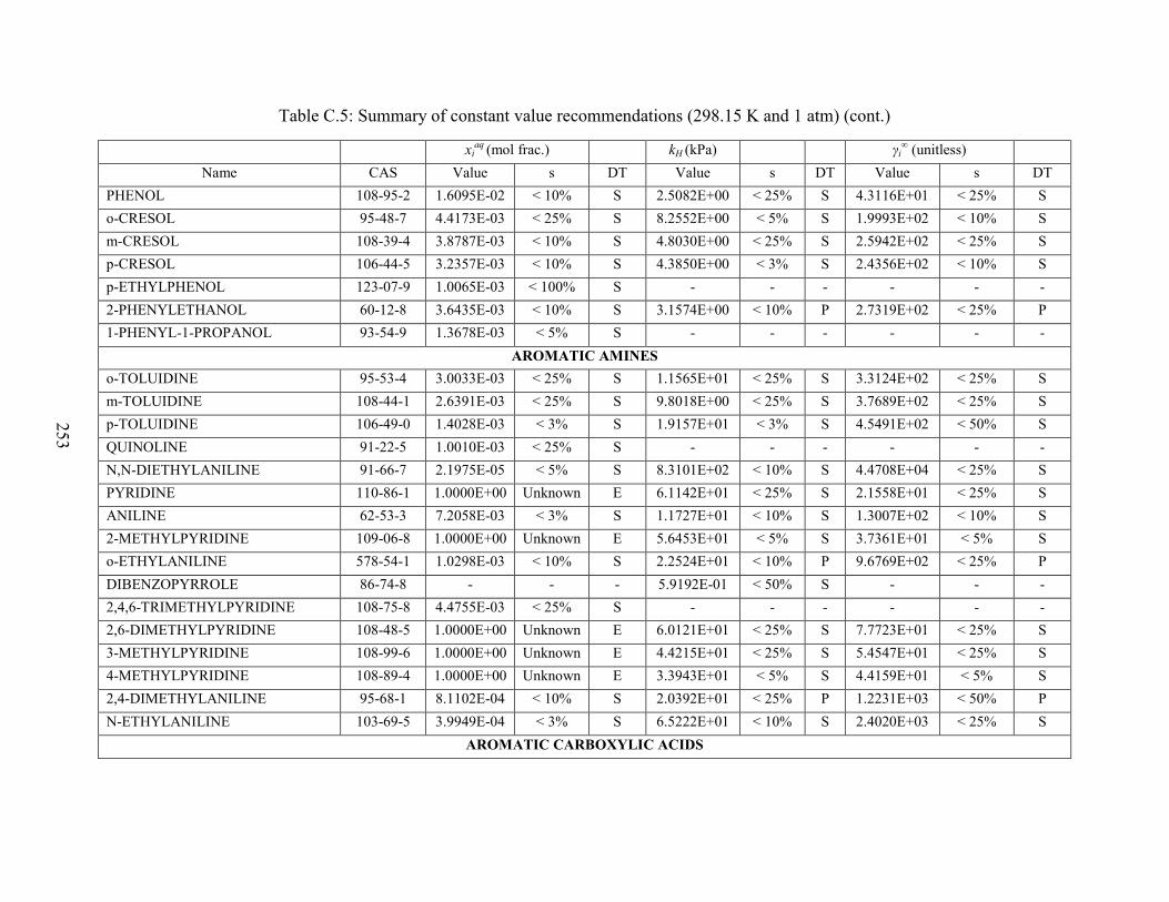
253

Table C.5: Summary of constant value recommendations (298.15 K and 1 atm) (cont.)

xiaq (mol frac.) kH (kPa) γi

∞ (unitless) Name CAS Value s DT Value s DT Value s DT

PHENOL 108-95-2 1.6095E-02 < 10% S 2.5082E+00 < 25% S 4.3116E+01 < 25% S o-CRESOL 95-48-7 4.4173E-03 < 25% S 8.2552E+00 < 5% S 1.9993E+02 < 10% S m-CRESOL 108-39-4 3.8787E-03 < 10% S 4.8030E+00 < 25% S 2.5942E+02 < 25% S p-CRESOL 106-44-5 3.2357E-03 < 10% S 4.3850E+00 < 3% S 2.4356E+02 < 10% S p-ETHYLPHENOL 123-07-9 1.0065E-03 < 100% S - - - - - - 2-PHENYLETHANOL 60-12-8 3.6435E-03 < 10% S 3.1574E+00 < 10% P 2.7319E+02 < 25% P 1-PHENYL-1-PROPANOL 93-54-9 1.3678E-03 < 5% S - - - - - -

AROMATIC AMINES o-TOLUIDINE 95-53-4 3.0033E-03 < 25% S 1.1565E+01 < 25% S 3.3124E+02 < 25% S m-TOLUIDINE 108-44-1 2.6391E-03 < 25% S 9.8018E+00 < 25% S 3.7689E+02 < 25% S p-TOLUIDINE 106-49-0 1.4028E-03 < 3% S 1.9157E+01 < 3% S 4.5491E+02 < 50% S QUINOLINE 91-22-5 1.0010E-03 < 25% S - - - - - - N,N-DIETHYLANILINE 91-66-7 2.1975E-05 < 5% S 8.3101E+02 < 10% S 4.4708E+04 < 25% S PYRIDINE 110-86-1 1.0000E+00 Unknown E 6.1142E+01 < 25% S 2.1558E+01 < 25% S ANILINE 62-53-3 7.2058E-03 < 3% S 1.1727E+01 < 10% S 1.3007E+02 < 10% S 2-METHYLPYRIDINE 109-06-8 1.0000E+00 Unknown E 5.6453E+01 < 5% S 3.7361E+01 < 5% S o-ETHYLANILINE 578-54-1 1.0298E-03 < 10% S 2.2524E+01 < 10% P 9.6769E+02 < 25% P DIBENZOPYRROLE 86-74-8 - - - 5.9192E-01 < 50% S - - - 2,4,6-TRIMETHYLPYRIDINE 108-75-8 4.4755E-03 < 25% S - - - - - - 2,6-DIMETHYLPYRIDINE 108-48-5 1.0000E+00 Unknown E 6.0121E+01 < 25% S 7.7723E+01 < 25% S 3-METHYLPYRIDINE 108-99-6 1.0000E+00 Unknown E 4.4215E+01 < 25% S 5.4547E+01 < 25% S 4-METHYLPYRIDINE 108-89-4 1.0000E+00 Unknown E 3.3943E+01 < 5% S 4.4159E+01 < 5% S 2,4-DIMETHYLANILINE 95-68-1 8.1102E-04 < 10% S 2.0392E+01 < 25% P 1.2231E+03 < 50% P N-ETHYLANILINE 103-69-5 3.9949E-04 < 3% S 6.5222E+01 < 10% S 2.4020E+03 < 25% S

AROMATIC CARBOXYLIC ACIDS

254

Table C.5: Summary of constant value recommendations (298.15 K and 1 atm) (cont.)

xiaq (mol frac.) kH (kPa) γi

∞ (unitless) Name CAS Value s DT Value s DT Value s DT

o-TOLUIC ACID 118-90-1 1.5612E-04 < 25% S - - - - - - p-TOLUIC ACID 99-94-5 4.6846E-05 < 5% S - - - - - - PHTHALIC ACID 88-99-3 6.9289E-04 < 5% S - - - - - - m-TOLUIC ACID 99-04-7 1.1411E-04 < 3% S - - - - - -

AROMATIC CHLORIDES BENZYL CHLORIDE 100-44-7 6.9223E-05 < 25% S 2.5098E+03 < 25% S 1.4426E+04 < 25% S MONOCHLOROBENZENE 108-90-7 7.3850E-05 < 5% S 2.1129E+04 < 5% S 1.3325E+04 < 10% S o-DICHLOROBENZENE 95-50-1 1.7571E-05 < 10% S 1.0267E+04 < 10% S 5.6832E+04 < 10% S m-DICHLOROBENZENE 541-73-1 1.5956E-05 < 10% S 1.7908E+04 < 10% S 6.2774E+04 < 10% S p-DICHLOROBENZENE 106-46-7 9.8562E-06 < 10% S 1.3908E+04 < 10% S 5.5428E+04 < 10% S HEXACHLOROBENZENE 118-74-1 3.6635E-10 < 25% S 8.4566E+03 < 25% S 1.8179E+08 < 100% S o-CHLOROTOLUENE 95-49-8 1.8949E-05 < 25% S 2.4693E+04 < 25% S 5.2836E+04 < 25% S p-CHLOROTOLUENE 106-43-4 1.7936E-05 < 25% S 2.0445E+04 < 25% S 5.5321E+04 < 25% S 2,4-DICHLOROTOLUENE 95-73-8 2.9825E-06 < 5% S 2.0337E+04 < 5% S 3.3512E+05 < 10% S 1,2,4-TRICHLOROBENZENE 120-82-1 4.0753E-06 < 25% S 1.3112E+04 < 25% S 2.5357E+05 < 25% S 1,2,3-TRICHLOROBENZENE 87-61-6 2.0122E-06 < 10% S 8.9256E+03 < 10% S 2.9730E+05 < 25% S

AROMATIC ESTERS BENZYL ACETATE 140-11-4 3.0871E-04 < 5% S 6.5097E+01 < 10% S 3.1178E+03 < 25% S DI-n-PROPYL PHTHALATE 131-16-8 6.6314E-06 < 25% S 2.5555E+00 < 25% S 1.5080E+05 < 25% S DI-n-HEXYL PHTHALATE 84-75-3 1.2643E-08 < 50% S 6.6872E+00 < 50% S 7.9098E+07 < 50% S METHYL BENZOATE 93-58-3 2.7549E-04 < 25% S 1.8175E+02 < 25% S 3.6117E+03 < 25% S ETHYL BENZOATE 93-89-0 1.1434E-04 < 25% S 3.3110E+02 < 25% S 8.7005E+03 < 25% S BENZYL FORMATE 104-57-4 1.2812E-03 < 25% S 2.8015E+01 < 10% S 6.8470E+02 < 25% S DIETHYL PHTHALATE 84-66-2 7.5610E-05 < 10% S 8.9347E-01 < 5% S 1.3457E+04 < 25% S DI-n-BUTYL PHTHALATE 84-74-2 6.4443E-07 < 25% S 5.2831E+00 < 25% S 1.5514E+06 < 25% S

255

Table C.5: Summary of constant value recommendations (298.15 K and 1 atm) (cont.)

xiaq (mol frac.) kH (kPa) γi

∞ (unitless) Name CAS Value s DT Value s DT Value s DT

DIMETHYL PHTHALATE 131-11-3 4.1370E-04 < 5% S 1.1053E+00 < 5% P 2.4220E+03 < 25% P C, H, BR COMPOUNDS

BROMOMETHANE 74-83-9 2.6893E-03 < 25% S 3.7821E+04 < 25% S - - - BROMOETHANE 74-96-4 1.5050E-03 < 3% S 4.1374E+04 < 3% S 6.6333E+02 < 10% S 1,1,2,2-TETRABROMOETHANE 79-27-6 1.5750E-06 < 50% S 3.8812E+03 < 100% S 6.3403E+05 < 100% S 1-BROMOPROPANE 106-94-5 3.5257E-04 < 3% S 5.2435E+04 < 3% S 2.8283E+03 < 5% S 2-BROMOPROPANE 75-26-3 4.6986E-04 < 3% S 6.1437E+04 < 3% S 2.1294E+03 < 5% S 1-BROMOBUTANE 109-65-9 7.4063E-05 < 25% S 7.4474E+04 < 25% S 1.3502E+04 < 25% S 1-BROMOHEPTANE 629-04-9 7.4417E-07 < 25% S 2.4825E+05 < 25% S 1.3438E+06 < 25% S 1,2-DIBROMOETHANE 106-93-4 4.2706E-04 < 10% S 4.0636E+03 < 10% S 2.3308E+03 < 10% S m-DIBROMOBENZENE 108-36-1 7.5328E-06 < 25% E 4.7500E+03 < 25% D 1.3275E+05 < 25% D BROMOBENZENE 108-86-1 4.5894E-05 < 5% S 1.2337E+04 < 5% S 2.1731E+04 < 10% S TRIBROMOMETHANE 75-25-2 2.4116E-04 < 5% S 3.0319E+03 < 10% S 4.1402E+03 < 10% S DIBROMOMETHANE 74-95-3 1.2397E-03 < 3% S 4.8569E+03 < 3% S 8.0641E+02 < 5% S 2-BROMOBUTANE 78-76-2 1.2019E-04 < 10% D 6.3195E+04 < 10% D 8.3200E+03 < 10% E p-BROMOTOLUENE 106-38-7 1.1174E-05 < 25% S 1.5321E+04 < 25% S 8.4309E+04 < 50% S

C, H, F COMPOUNDS METHYL FLUORIDE 593-53-3 1.0604E-03 < 1% S 9.5359E+04 < 3% S - - - PERFLUORO-n-HEXANE 355-42-0 4.8787E-09 < 100% E 5.9661E+09 < 100% D 2.0497E+08 < 100% D PERFLUORO-n-OCTANE 307-34-6 6.8663E-11 < 100% E 6.8797E+10 < 100% D 1.4564E+10 < 100% D 1,2-DIFLUOROBENZENE 367-11-3 1.6957E-04 < 25% S 4.2141E+04 < 25% S 5.8883E+03 < 25% S FLUOROBENZENE 462-06-6 2.7647E-04 < 10% S 3.7174E+04 < 10% S 3.6155E+03 < 10% S HEXAFLUOROBENZENE 392-56-3 6.0415E-05 < 3% S 1.8597E+05 < 3% S 1.6515E+04 < 5% S PERFLUORO-n-PENTANE 678-26-2 7.2276E-08 < 100% E 1.2114E+09 < 100% D 1.3835E+07 < 100% D PERFLUORO-n-HEPTANE 335-57-9 5.6014E-10 < 100% E 1.8284E+10 < 100% D 1.7852E+09 < 100% D

256

Table C.5: Summary of constant value recommendations (298.15 K and 1 atm) (cont.)

xiaq (mol frac.) kH (kPa) γi

∞ (unitless) Name CAS Value s DT Value s DT Value s DT

C, H, I COMPOUNDS METHYL IODIDE 74-88-4 1.8484E-03 < 5% S 2.9424E+04 < 5% S 5.4150E+02 < 10% S ETHYL IODIDE 75-03-6 4.6009E-04 < 3% S 3.8621E+04 < 3% S 2.1744E+03 < 10% S n-PROPYL IODIDE 107-08-4 1.0973E-04 < 5% S 5.2297E+04 < 5% S 9.0990E+03 < 10% S ISOPROPYL IODIDE 75-30-9 1.4480E-04 < 10% S 6.5461E+04 < 5% S 6.8884E+03 < 10% S IODOBENZENE 591-50-4 1.9110E-05 < 10% S 7.3212E+03 < 25% S 5.1681E+04 < 25% S n-HEXYL IODIDE 638-45-9 1.1954E-06 < 25% S 1.6347E+05 < 25% S 8.3652E+05 < 25% S n-BUTYL IODIDE 542-69-8 2.2740E-05 < 10% S 8.0572E+04 < 25% S 4.3976E+04 < 10% S

C, H, MULTIHALOGEN COMPOUNDS DICHLORODIFLUOROMETHANE 75-71-8 5.4251E-05 < 3% S 1.8669E+06 < 10% S - - - TRICHLOROFLUOROMETHANE 75-69-4 - - - 5.2851E+05 < 10% S - - - 1,1,2-TRICHLOROTRIFLUOROETHANE

76-13-1 2.3783E-05 < 25% S 1.8719E+06 < 25% S 4.2032E+04 < 25% S

C, H, NO2 COMPOUNDS NITROMETHANE 75-52-5 3.2090E-02 < 10% S 1.4923E+02 < 10% S 3.1049E+01 < 10% S NITROETHANE 79-24-3 1.0659E-02 < 5% S 2.5784E+02 < 5% S 9.3542E+01 < 10% S 1-NITROPROPANE 108-03-2 3.2369E-03 < 5% S 4.1378E+02 < 5% S 3.0767E+02 < 10% S 2-NITROPROPANE 79-46-9 3.5066E-03 < 5% S 6.5009E+02 < 3% S 2.8516E+02 < 10% S 1-NITROBUTANE 627-05-4 6.5301E-04 < 25% S 7.2451E+02 < 25% S 1.5314E+03 < 25% S o-NITROTOLUENE 88-72-2 8.4414E-05 < 5% S 2.3476E+02 < 10% S 1.1833E+04 < 10% S p-NITROTOLUENE 99-99-0 4.6972E-05 < 10% S 6.2304E+01 < 10% S 1.2362E+04 < 50% S m-NITROTOLUENE 99-08-1 6.6378E-05 < 5% S 2.0274E+02 < 10% S 1.4420E+04 < 25% S NITROBENZENE 98-95-3 2.8289E-04 < 5% S 1.1835E+02 < 5% S 3.5294E+03 < 10% S m-DINITROBENZENE 99-65-0 5.7572E-05 < 10% S - - - - - - p-DINITROBENZENE 100-25-4 6.6100E-06 < 3% S - - - - - -

257

Table C.5: Summary of constant value recommendations (298.15 K and 1 atm) (cont.)

xiaq (mol frac.) kH (kPa) γi

∞ (unitless) Name CAS Value s DT Value s DT Value s DT

2,4-DINITROTOLUENE 121-14-2 1.9749E-05 < 5% S 1.4084E+00 < 5% S 1.6382E+04 < 25% S 2,6-DINITROTOLUENE 606-20-2 2.0406E-05 < 5% S 1.1571E+01 < 3% S 2.3491E+04 < 50% S 3,4-DINITROTOLUENE 610-39-9 1.6997E-05 < 5% S 1.6741E+00 < 5% S 2.6088E+04 < 50% S 2,4,6-TRINITROTOLUENE 118-96-7 9.5510E-06 < 5% S 1.2083E-01 < 5% S 2.1202E+04 < 50% S RDX 121-82-4 3.9683E-06 < 5% S - - - - - - HMX 2691-41-0 2.7726E-07 < 10% S - - - - - -

C1/C2 ALIPHATIC CHLORIDES CARBON TETRACHLORIDE 56-23-5 9.0660E-05 < 5% S 1.6765E+05 < 5% S 1.1029E+04 < 5% S METHYL CHLORIDE 74-87-3 1.9096E-03 < 10% S 5.2937E+04 < 10% S - - - ETHYL CHLORIDE 75-00-3 1.5332E-03 < 25% S 6.6090E+04 < 10% S - - - VINYL CHLORIDE 75-01-4 7.7389E-04 < 25% S 1.3062E+05 < 25% S - - - DICHLOROMETHANE 75-09-2 4.0143E-03 < 10% S 1.4546E+04 < 10% S 2.4938E+02 < 10% S CHLOROFORM 67-66-3 1.1812E-03 < 3% S 2.2108E+04 < 3% S 8.4620E+02 < 5% S 1,1-DICHLOROETHANE 75-34-3 9.3878E-04 < 5% S 3.2146E+04 < 5% S 1.0626E+03 < 5% S 1,2-DICHLOROETHANE 107-06-2 1.5990E-03 < 5% S 6.6406E+03 < 5% S 6.2532E+02 < 5% S 1,1,2-TRICHLOROETHANE 79-00-5 6.2690E-04 < 5% S 4.9329E+03 < 5% S 1.5984E+03 < 5% S HEXACHLOROETHANE 67-72-1 2.9288E-06 < 25% S 2.0130E+04 < 25% S 1.6173E+05 > 100% S 1,1,1-TRICHLOROETHANE 71-55-6 1.7505E-04 < 5% S 9.4916E+04 < 5% S 5.7096E+03 < 10% S 1,1,1,2-TETRACHLOROETHANE 630-20-6 1.1099E-04 < 10% S 1.3082E+04 < 10% S 8.2197E+03 < 10% S 1,1,2,2-TETRACHLOROETHANE 79-34-5 3.1284E-04 < 10% S 2.3451E+03 < 10% S 3.0753E+03 < 10% S TRICHLOROETHYLENE 79-01-6 1.8045E-04 < 3% S 5.4319E+04 < 3% S 5.5283E+03 < 5% S TETRACHLOROETHYLENE 127-18-4 2.4977E-05 < 5% S 9.8707E+04 < 5% S 3.9944E+04 < 10% S cis-1,2-DICHLOROETHYLENE 156-59-2 1.1760E-03 < 10% S 2.3105E+04 < 10% S 8.4974E+02 < 10% S trans-1,2-DICHLOROETHYLENE 156-60-5 8.2754E-04 < 10% S 5.3633E+04 < 10% S 1.2109E+03 < 10% S PENTACHLOROETHANE 76-01-7 3.6884E-05 < 25% S 1.3266E+04 < 25% S 2.7105E+04 < 25% S

258

Table C.5: Summary of constant value recommendations (298.15 K and 1 atm) (cont.)

xiaq (mol frac.) kH (kPa) γi

∞ (unitless) Name CAS Value s DT Value s DT Value s DT

1,1-DICHLOROETHYLENE 75-35-4 4.6806E-04 < 10% S 1.7069E+05 < 10% S 2.1390E+03 < 10% S C3 & HIGHER ALIPHATIC CHLORIDES

1,4-DICHLOROBUTANE 110-56-5 1.8176E-04 < 25% S 2.7961E+03 < 10% S 5.4994E+03 < 25% S 1,5-DICHLOROPENTANE 628-76-2 2.5038E-05 < 100% S 5.3788E+03 < 100% S 3.9925E+04 < 100% S 1,2-DICHLOROPROPANE 78-87-5 4.3120E-04 < 5% S 1.6001E+04 < 5% S 2.3227E+03 < 10% S ISOPROPYL CHLORIDE 75-29-6 7.1457E-04 < 10% S 9.6129E+04 < 5% S 1.3976E+03 < 10% S 1,2,3-TRICHLOROPROPANE 96-18-4 2.8896E-04 < 25% S 1.6851E+03 < 25% S 3.4614E+03 < 25% S HEXACHLORO-1,3-BUTADIENE 87-68-3 3.1189E-07 < 50% S 9.8863E+04 < 50% S 3.1995E+06 < 50% S PROPYL CHLORIDE 540-54-5 6.3068E-04 < 10% S 7.2709E+04 < 10% S 1.5838E+03 < 10% S n-BUTYL CHLORIDE 109-69-3 1.3685E-04 < 10% S 9.8517E+04 < 10% S 7.3035E+03 < 10% S sec-BUTYL CHLORIDE 78-86-4 1.5548E-04 < 10% S 1.3477E+05 < 10% S 6.4263E+03 < 10% S 1-CHLOROPENTANE 543-59-9 3.3579E-05 < 5% S 1.2764E+05 < 5% S 2.9802E+04 < 5% S 1,3-DICHLOROPROPANE 142-28-9 3.7373E-04 < 25% S 4.7562E+03 < 25% S 2.6752E+03 < 25% S

CYCLOALIPHATIC ALCOHOLS CYCLOHEXANOL 108-93-0 6.9303E-03 < 5% S 1.2847E+01 < 50% S 1.4416E+02 < 50% S

CYCLOALKANES CYCLOPENTANE 287-92-3 4.3311E-05 < 10% S 9.8100E+05 < 10% S 2.3099E+04 < 10% S CYCLOHEXANE 110-82-7 1.3004E-05 < 10% S 9.4972E+05 < 10% S 7.2858E+04 < 10% S CYCLOHEPTANE 291-64-5 3.5216E-06 < 10% P 8.2667E+05 < 10% P 2.8396E+05 < 10% P CYCLOOCTANE 292-64-8 9.7862E-07 < 10% S 7.6345E+05 < 10% S 1.0159E+06 < 10% S

CYCLOALKENES CYCLOPENTENE 142-29-0 1.7784E-04 < 50% S 2.8372E+05 < 50% S 5.6203E+03 < 50% S CYCLOHEXENE 110-83-8 6.2535E-05 < 10% S 1.8948E+05 < 10% S 1.5966E+04 < 10% S CYCLOHEPTENE 628-92-2 1.2363E-05 < 10% E 2.7050E+05 < 25% D 8.0884E+04 < 10% D CYCLOOCTENE 931-88-4 3.8290E-06 < 3% S 2.6909E+05 < 3% S 2.6479E+05 < 3% S

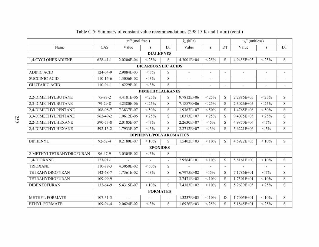
259

Table C.5: Summary of constant value recommendations (298.15 K and 1 atm) (cont.)

xiaq (mol frac.) kH (kPa) γi

∞ (unitless) Name CAS Value s DT Value s DT Value s DT

DIALKENES 1,4-CYCLOHEXADIENE 628-41-1 2.0206E-04 < 25% S 4.3001E+04 < 25% S 4.9455E+03 < 25% S

DICARBOXYLIC ACIDS ADIPIC ACID 124-04-9 2.9884E-03 < 3% S - - - - - - SUCCINIC ACID 110-15-6 1.3056E-02 < 3% S - - - - - - GLUTARIC ACID 110-94-1 1.6229E-01 < 3% S - - - - - -

DIMETHYLALKANES 2,2-DIMETHYLBUTANE 75-83-2 4.4181E-06 < 25% S 9.7812E+06 < 25% S 2.2886E+05 < 25% S 2,3-DIMETHYLBUTANE 79-29-8 4.2380E-06 < 25% S 7.1887E+06 < 25% S 2.3026E+05 < 25% S 2,4-DIMETHYLPENTANE 108-08-7 7.3837E-07 < 50% S 1.9367E+07 < 50% S 1.4765E+06 < 50% S 3,3-DIMETHYLPENTANE 562-49-2 1.0612E-06 < 25% S 1.0373E+07 < 25% S 9.4075E+05 < 25% S 2,2-DIMETHYLHEXANE 590-73-8 2.0105E-07 < 3% S 2.2630E+07 < 5% S 4.9870E+06 < 5% S 2,5-DIMETHYLHEXANE 592-13-2 1.7933E-07 < 3% S 2.2712E+07 < 3% S 5.6221E+06 < 5% S

DIPHENYL/POLYAROMATICS BIPHENYL 92-52-4 8.2180E-07 < 10% S 1.5402E+03 < 10% S 4.5922E+05 < 10% S

EPOXIDES 2-METHYLTETRAHYDROFURAN 96-47-9 3.0305E-02 < 5% S - - - - - - 1,4-DIOXANE 123-91-1 - - - 2.9564E+01 < 10% S 5.8161E+00 < 10% S TRIOXANE 110-88-3 4.3058E-02 < 50% S - - - - - - TETRAHYDROPYRAN 142-68-7 1.7361E-02 < 3% S 6.7975E+02 < 5% S 7.1786E+01 < 5% S TETRAHYDROFURAN 109-99-9 - - - 3.7471E+02 < 10% S 1.7501E+01 < 10% S DIBENZOFURAN 132-64-9 5.4315E-07 < 10% S 7.4383E+02 < 10% S 5.2639E+05 < 25% S

FORMATES METHYL FORMATE 107-31-3 - - - 1.3237E+03 < 10% D 1.7005E+01 < 10% S ETHYL FORMATE 109-94-4 2.0624E-02 < 3% S 1.6926E+03 < 25% S 5.1845E+01 < 25% S

260

Table C.5: Summary of constant value recommendations (298.15 K and 1 atm) (cont.)

xiaq (mol frac.) kH (kPa) γi

∞ (unitless) Name CAS Value s DT Value s DT Value s DT

n-PROPYL FORMATE 110-74-7 5.6073E-03 < 5% S 1.8180E+03 < 10% S 1.6754E+02 < 10% S n-BUTYL FORMATE 592-84-7 1.7728E-03 < 25% S 2.1415E+03 < 25% P 5.6349E+02 < 25% P ISOBUTYL FORMATE 542-55-2 1.5568E-03 < 10% S 3.3686E+03 < 10% S 6.1884E+02 < 10% P n-PENTYL FORMATE 638-49-3 3.8458E-04 < 25% S 3.0716E+03 < 25% S 2.5812E+03 < 25% S tert-BUTYL FORMATE 762-75-4 2.8541E-03 < 5% S 3.8948E+03 < 5% S 3.5011E+02 < 25% S

KETONES ACETONE 67-64-1 - - - 1.9892E+02 < 5% S 6.4743E+00 < 10% S METHYL ETHYL KETONE 78-93-3 8.0636E-02 < 3% S 3.0126E+02 < 10% S 2.4485E+01 < 10% S 3-PENTANONE 96-22-0 1.0287E-02 < 10% S 5.8894E+02 < 5% S 9.7081E+01 < 10% S METHYL ISOBUTYL KETONE 108-10-1 3.2450E-03 < 10% S 8.1503E+02 < 10% S 3.0755E+02 < 25% S 3-HEPTANONE 106-35-4 7.1140E-04 < 10% S 7.8587E+02 < 10% S 1.3989E+03 < 25% S 4-HEPTANONE 123-19-3 6.5059E-04 < 10% S 1.1765E+03 < 10% S 1.5279E+03 < 25% S 3-HEXANONE 589-38-8 2.6395E-03 < 25% S 7.0108E+02 < 10% S 3.7866E+02 < 10% S 2-PENTANONE 107-87-9 1.1528E-02 < 5% S 4.0969E+02 < 5% S 8.6500E+01 < 10% S METHYL ISOPROPYL KETONE 563-80-4 1.3715E-02 < 5% S 5.1455E+02 < 5% P 7.4588E+01 < 10% P 2-HEXANONE 591-78-6 2.8457E-03 < 5% S 5.4080E+02 < 5% S 3.4847E+02 < 10% S 2-HEPTANONE 110-43-0 6.4445E-04 < 3% S 8.0639E+02 < 3% S 1.5469E+03 < 5% P 5-METHYL-2-HEXANONE 110-12-3 7.7380E-04 < 5% S 8.8878E+02 < 5% S 1.2828E+03 < 5% S 3,3-DIMETHYL-2-BUTANONE 75-97-8 3.4404E-03 < 5% S 1.2372E+03 < 5% S 2.8979E+02 < 25% S DIISOBUTYL KETONE 108-83-8 5.1396E-05 < 10% S 4.3295E+03 < 10% S 1.9301E+04 < 10% S DIISOPROPYL KETONE 565-80-0 7.8573E-04 < 10% S 2.4265E+03 < 10% S 1.2694E+03 < 25% S 5-NONANONE 502-56-7 5.6855E-05 < 25% S 1.3894E+03 < 25% S 1.7526E+04 < 25% S 2-NONANONE 821-55-6 4.2752E-05 < 25% S 1.5963E+03 < 25% S 2.3810E+04 < 25% S ACETYLACETONE 123-54-6 3.3792E-02 < 5% S 6.4870E+01 < 25% S 4.9594E+01 < 50% S ISOPHORONE 78-59-1 1.8712E-03 < 3% S - - - - - -

261

Table C.5: Summary of constant value recommendations (298.15 K and 1 atm) (cont.)

xiaq (mol frac.) kH (kPa) γi

∞ (unitless) Name CAS Value s DT Value s DT Value s DT

CYCLOPENTANONE 120-92-3 8.0153E-02 < 3% S 4.4727E+01 < 100% S 2.9473E+01 < 100% S CYCLOHEXANONE 108-94-1 1.7464E-02 < 5% S 3.6312E+01 < 25% S 6.4858E+01 < 25% S 2-OCTANONE 111-13-7 1.8040E-04 < 25% S 1.0319E+03 < 25% S 5.5108E+03 < 25% S ACETOPHENONE 98-86-2 9.1777E-04 < 25% S 5.0333E+01 < 25% S 9.5225E+02 < 25% S 3-OCTANONE 106-68-3 1.8418E-04 < 10% S 1.3047E+03 < 10% S 5.4089E+03 < 25% S 3-NONANONE 925-78-0 6.3260E-05 < 25% S 1.0827E+03 < 25% S 1.5675E+04 < 25% S 2,6,8-TRIMETHYL-4-NONANONE 123-18-2 2.2065E-06 < 25% P 5.2094E+03 < 25% P 4.5321E+05 < 25% P

MERCAPTANS ISOPROPYL MERCAPTAN 75-33-2 8.7844E-04 < 10% S 4.1922E+04 < 10% S 1.1366E+03 < 10% S n-BUTYL MERCAPTAN 109-79-5 1.6284E-04 < 3% S 3.7378E+04 < 5% S 6.0435E+03 < 10% S

METHYLALKANES 2-METHYLPENTANE 107-83-5 3.0912E-06 < 25% S 8.9514E+06 < 10% S 3.1860E+05 < 25% S 3-METHYLPENTANE 96-14-0 2.7067E-06 < 3% S 9.3257E+06 < 3% S 3.6949E+05 < 3% S 2-METHYLHEXANE 591-76-4 4.5667E-07 < 5% E 1.9204E+07 < 10% D 2.1898E+06 < 5% D 3-METHYLHEXANE 589-34-4 4.7716E-07 < 5% S 1.7157E+07 < 10% S 2.0958E+06 < 5% S 3-METHYLHEPTANE 589-81-1 1.2491E-07 < 5% E 2.0935E+07 < 10% S 8.0059E+06 < 10% S 4-METHYLHEPTANE 589-53-7 1.3224E-07 < 3% E 2.0657E+07 < 5% D 7.5617E+06 < 5% D

METHYLALKENES 2-METHYL-2-BUTENE 513-35-9 - - - 9.6127E+05 < 3% S - - -

N-ALCOHOLS METHANOL 67-56-1 - - - 2.8376E+01 < 5% S 1.6882E+00 < 5% S ETHANOL 64-17-5 - - - 3.1518E+01 < 5% S 3.9792E+00 < 5% S 1-PROPANOL 71-23-8 - - - 3.9058E+01 < 10% S 1.3915E+01 < 10% S 1-BUTANOL 71-36-3 1.8884E-02 < 3% S 4.7161E+01 < 5% S 5.2370E+01 < 10% S 1-PENTANOL 71-41-0 4.3266E-03 < 3% S 6.3569E+01 < 10% S 1.9216E+02 < 10% S

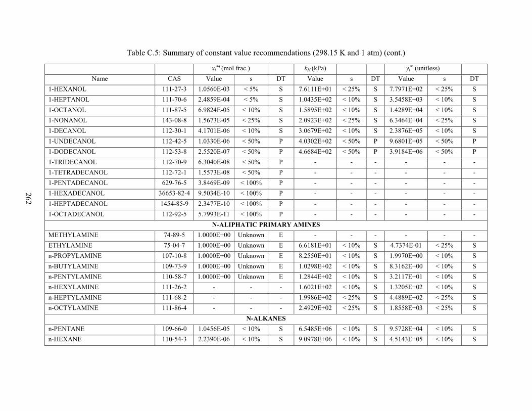
262

Table C.5: Summary of constant value recommendations (298.15 K and 1 atm) (cont.)

xiaq (mol frac.) kH (kPa) γi

∞ (unitless) Name CAS Value s DT Value s DT Value s DT

1-HEXANOL 111-27-3 1.0560E-03 < 5% S 7.6111E+01 < 25% S 7.7971E+02 < 25% S 1-HEPTANOL 111-70-6 2.4859E-04 < 5% S 1.0435E+02 < 10% S 3.5458E+03 < 10% S 1-OCTANOL 111-87-5 6.9824E-05 < 10% S 1.5895E+02 < 10% S 1.4289E+04 < 10% S 1-NONANOL 143-08-8 1.5673E-05 < 25% S 2.0923E+02 < 25% S 6.3464E+04 < 25% S 1-DECANOL 112-30-1 4.1701E-06 < 10% S 3.0679E+02 < 10% S 2.3876E+05 < 10% S 1-UNDECANOL 112-42-5 1.0330E-06 < 50% P 4.0302E+02 < 50% P 9.6801E+05 < 50% P 1-DODECANOL 112-53-8 2.5520E-07 < 50% P 4.6684E+02 < 50% P 3.9184E+06 < 50% P 1-TRIDECANOL 112-70-9 6.3040E-08 < 50% P - - - - - - 1-TETRADECANOL 112-72-1 1.5573E-08 < 50% P - - - - - - 1-PENTADECANOL 629-76-5 3.8469E-09 < 100% P - - - - - - 1-HEXADECANOL 36653-82-4 9.5034E-10 < 100% P - - - - - - 1-HEPTADECANOL 1454-85-9 2.3477E-10 < 100% P - - - - - - 1-OCTADECANOL 112-92-5 5.7993E-11 < 100% P - - - - - -

N-ALIPHATIC PRIMARY AMINES METHYLAMINE 74-89-5 1.0000E+00 Unknown E - - - - - - ETHYLAMINE 75-04-7 1.0000E+00 Unknown E 6.6181E+01 < 10% S 4.7374E-01 < 25% S n-PROPYLAMINE 107-10-8 1.0000E+00 Unknown E 8.2550E+01 < 10% S 1.9970E+00 < 10% S n-BUTYLAMINE 109-73-9 1.0000E+00 Unknown E 1.0298E+02 < 10% S 8.3162E+00 < 10% S n-PENTYLAMINE 110-58-7 1.0000E+00 Unknown E 1.2844E+02 < 10% S 3.2117E+01 < 10% S n-HEXYLAMINE 111-26-2 - - - 1.6021E+02 < 10% S 1.3205E+02 < 10% S n-HEPTYLAMINE 111-68-2 - - - 1.9986E+02 < 25% S 4.4889E+02 < 25% S n-OCTYLAMINE 111-86-4 - - - 2.4929E+02 < 25% S 1.8558E+03 < 25% S

N-ALKANES n-PENTANE 109-66-0 1.0456E-05 < 10% S 6.5485E+06 < 10% S 9.5728E+04 < 10% S n-HEXANE 110-54-3 2.2390E-06 < 10% S 9.0978E+06 < 10% S 4.5143E+05 < 10% S

263

Table C.5: Summary of constant value recommendations (298.15 K and 1 atm) (cont.)

xiaq (mol frac.) kH (kPa) γi

∞ (unitless) Name CAS Value s DT Value s DT Value s DT

n-HEPTANE 142-82-5 4.7371E-07 < 10% S 1.2916E+07 < 10% S 2.1361E+06 < 10% S n-OCTANE 111-65-9 1.1329E-07 < 25% S 1.6258E+07 < 25% S 8.7203E+06 < 25% S n-NONANE 111-84-2 1.8576E-08 < 50% S 3.0731E+07 < 50% S 5.2941E+07 < 50% S n-DECANE 124-18-5 4.3460E-09 < 50% S 4.1648E+07 < 50% S 2.3009E+08 < 50% S

N-ALKYLBENZENES BENZENE 71-43-2 4.0652E-04 < 3% S 3.1114E+04 < 3% S 2.4561E+03 < 3% S TOLUENE 108-88-3 1.1535E-04 < 3% S 3.3054E+04 < 3% S 8.6874E+03 < 5% S ETHYLBENZENE 100-41-4 2.9892E-05 < 3% S 4.2613E+04 < 3% S 3.3370E+04 < 5% S n-PROPYLBENZENE 103-65-1 7.7818E-06 < 10% S 5.9359E+04 < 10% S 1.2796E+05 < 10% S n-BUTYLBENZENE 104-51-8 1.8154E-06 < 5% S 7.8555E+04 < 5% S 5.4877E+05 < 5% S n-HEPTYLBENZENE 1078-71-3 2.3098E-08 < 5% P 2.0792E+05 < 10% P 4.3293E+07 < 5% P n-DECYLBENZENE 104-72-3 2.0688E-10 < 10% S 7.2846E+05 < 10% S 4.8338E+09 < 10% S n-PENTYLBENZENE 538-68-1 4.3812E-07 < 10% S 1.0026E+05 < 10% S 2.2824E+06 < 10% S n-HEXYLBENZENE 1077-16-3 1.0832E-07 < 3% S 1.3470E+05 < 5% S 9.2359E+06 < 10% S n-OCTYLBENZENE 2189-60-8 4.9663E-09 < 10% P 3.0050E+05 < 10% P 2.0136E+08 < 10% P n-NONYLBENZENE 1081-77-2 1.0313E-09 < 10% P 3.8660E+05 < 25% P 9.6961E+08 < 10% P

NAPHTHALENES NAPHTHALENE 91-20-3 4.3668E-06 < 3% S 2.5234E+03 < 3% S 7.0849E+04 < 5% S 1-METHYLNAPHTHALENE 90-12-0 3.6833E-06 < 10% S 2.7244E+03 < 10% S 2.7144E+05 < 10% S 2-METHYLNAPHTHALENE 91-57-6 3.0163E-06 < 25% S 2.7289E+03 < 25% S 2.8517E+05 < 25% S 1-ETHYLNAPHTHALENE 1127-76-0 1.1956E-06 < 10% S 2.7757E+03 < 10% S 8.3651E+05 < 10% S

NITRILES ACETONITRILE 75-05-8 - - - 1.1210E+02 < 5% S 9.2319E+00 < 5% S PROPIONITRILE 107-12-0 3.5087E-02 < 10% S 1.6565E+02 < 25% S 2.6265E+01 < 25% S ACRYLONITRILE 107-13-1 2.3502E-02 < 3% S 5.4807E+02 < 3% S 4.1682E+01 < 25% S

264

Table C.5: Summary of constant value recommendations (298.15 K and 1 atm) (cont.)

xiaq (mol frac.) kH (kPa) γi

∞ (unitless) Name CAS Value s DT Value s DT Value s DT

METHACRYLONITRILE 126-98-7 5.9311E-03 < 5% S 1.5916E+03 < 5% P 1.6780E+02 < 10% P SUCCINONITRILE 110-61-2 2.2642E-02 < 10% S - - - - - - GLUTARONITRILE 544-13-8 1.9661E-02 < 10% S - - - - - - n-BUTYRONITRILE 109-74-0 8.8648E-03 < 3% S 2.9080E+02 < 3% S 1.1185E+02 < 5% S VALERONITRILE 110-59-8 2.7594E-03 < 10% S 3.5359E+02 < 25% S 3.6302E+02 < 25% S ISOBUTYRONITRILE 78-82-0 9.2527E-03 < 5% S 5.0410E+02 < 25% S 1.1538E+02 < 25% S BENZONITRILE 100-47-0 7.1412E-04 < 25% S 1.6637E+02 < 25% S 1.5605E+03 < 25% S VINYLACETONITRILE 109-75-1 8.8683E-03 < 5% S 2.7177E+02 < 1% S 1.1032E+02 < 5% S PHENYLACETONITRILE 140-29-4 2.6710E-04 < 25% S 5.0250E+01 < 100% S 4.0865E+03 < 100% S

NITROAMINES o-NITROANILINE 88-74-4 1.3507E-04 < 50% S 7.7514E-01 < 50% S 3.3338E+03 < 100% S p-NITROANILINE 100-01-6 7.4078E-05 < 10% S 6.3686E-03 < 10% S 1.6454E+03 < 50% S m-NITROANILINE 99-09-2 1.2221E-04 < 10% S - - - - - -

ORGANIC SALTS DIETHYL CARBONATE 105-58-8 2.6923E-03 < 3% S 5.3166E+02 < 3% S 3.6990E+02 < 10% S DIMETHYL CARBONATE 616-38-6 2.7871E-02 < 3% S 3.5902E+02 < 3% S 4.8661E+01 < 5% S

OTHER ALIPHATIC ALCOHOLS ISOPROPANOL 67-63-0 - - - 4.8094E+01 < 10% S 8.2933E+00 < 10% S 2-METHYL-1-PROPANOL 78-83-1 2.1995E-02 < 10% S 6.7391E+01 < 10% S 4.8123E+01 < 10% S 2-BUTANOL 78-92-2 5.0591E-02 < 3% S 5.9124E+01 < 5% S 2.5291E+01 < 5% S 2-METHYL-2-PROPANOL 75-65-0 - - - 6.8926E+01 < 5% S 1.2064E+01 < 10% S 2-PENTANOL 6032-29-7 8.8835E-03 < 5% S 7.9763E+01 < 3% S 9.8222E+01 < 5% S 2-METHYL-2-BUTANOL 75-85-4 2.4227E-02 < 10% S 8.1409E+01 < 3% S 3.5808E+01 < 5% S 2-METHYL-1-BUTANOL 137-32-6 5.4588E-03 < 5% S 7.2382E+01 < 5% S 1.4816E+02 < 5% S 2,2-DIMETHYL-1-PROPANOL 75-84-3 6.8035E-03 < 10% S 1.7596E+02 < 25% P 1.3088E+02 < 25% P

265

Table C.5: Summary of constant value recommendations (298.15 K and 1 atm) (cont.)

xiaq (mol frac.) kH (kPa) γi

∞ (unitless) Name CAS Value s DT Value s DT Value s DT

2-HEXANOL 626-93-7 2.1193E-03 < 5% S 1.4331E+02 < 5% S 4.6989E+02 < 10% S 3-HEXANOL 623-37-0 2.7146E-03 < 5% S 1.5227E+02 < 3% S 3.6732E+02 < 25% S 3-METHYL-1-PENTANOL 589-35-5 1.6550E-03 < 3% S 7.6763E+01 < 10% P 5.9895E+02 < 10% P 3-METHYL-3-PENTANOL 77-74-7 6.1117E-03 < 10% S 2.1990E+02 < 10% P 1.6495E+02 < 25% P 3-PENTANOL 584-02-1 1.0665E-02 < 3% S 9.2713E+01 < 3% S 8.3949E+01 < 5% S 3-METHYL-1-BUTANOL 123-51-3 5.3033E-03 < 5% S 6.9731E+01 < 10% S 1.6643E+02 < 25% S 3-METHYL-2-BUTANOL 598-75-4 1.1849E-02 < 5% S 1.1070E+02 < 3% S 7.9081E+01 < 10% S 2-HEPTANOL 543-49-7 5.7725E-04 < 5% S 1.7236E+02 < 5% P 1.7183E+03 < 10% P 3-HEPTANOL 589-82-2 7.1191E-04 < 10% S 1.7651E+02 < 10% S 1.3947E+03 < 10% S 4-METHYL-2-PENTANOL 108-11-2 2.8026E-03 < 10% S 2.4972E+02 < 5% S 3.5580E+02 < 10% S 2-OCTANOL 123-96-6 1.5562E-04 < 10% S 2.1047E+02 < 10% P 6.3825E+03 < 10% P 2-NONANOL 628-99-9 3.8944E-05 < 25% S 2.7628E+02 < 25% P 2.5433E+04 < 25% P 2,6-DIMETHYL-4-HEPTANOL 108-82-7 7.5500E-05 < 25% S 5.3226E+02 < 25% P 1.3210E+04 < 25% P

OTHER ALIPHATIC AMINES DIMETHYLAMINE 124-40-3 - - - 8.9023E+01 < 50% S - - - TRIETHYLAMINE 121-44-8 1.4394E-02 < 10% S 5.9606E+02 < 5% S 6.5469E+01 < 5% S DI-n-PROPYLAMINE 142-84-7 7.1637E-03 < 25% S 2.5765E+02 < 25% S 7.1297E+01 < 25% S N,N-DIMETHYL-n-BUTYLAMINE 927-62-8 4.7045E-03 < 25% S - - - - - - N,N-DIETHYLMETHYLAMINE 616-39-7 1.0000E+00 Unknown E - - - - - - DIETHYLAMINE 109-89-7 1.0000E+00 Unknown E 1.5144E+02 < 25% S 4.8211E+00 < 25% S DIISOPROPYLAMINE 108-18-9 1.0000E+00 Unknown E - - - - - - DI-n-BUTYLAMINE 111-92-2 6.8942E-04 < 10% S 4.3834E+02 < 50% S 1.2008E+03 < 50% S TRI-n-BUTYLAMINE 102-82-9 8.1648E-05 < 25% S 1.4890E+02 < 25% S 1.2208E+04 < 25% S

OTHER ALKANES 2,3,4-TRIMETHYLPENTANE 565-75-3 2.1260E-07 < 5% S 1.7009E+07 < 5% S 4.7045E+06 < 5% S

266

Table C.5: Summary of constant value recommendations (298.15 K and 1 atm) (cont.)

xiaq (mol frac.) kH (kPa) γi

∞ (unitless) Name CAS Value s DT Value s DT Value s DT

2,2,5-TRIMETHYLHEXANE 3522-94-9 7.5851E-08 < 5% E 2.9316E+07 < 10% D 1.3113E+07 < 10% D OTHER ALKYLBENZENES

o-XYLENE 95-47-6 3.2745E-05 < 10% S 2.7047E+04 < 10% S 3.0533E+04 < 10% S m-XYLENE 108-38-3 2.8685E-05 < 5% S 3.8659E+04 < 5% S 3.4498E+04 < 10% S p-XYLENE 106-42-3 2.9633E-05 < 10% S 3.8088E+04 < 10% S 3.2575E+04 < 10% S CUMENE 98-82-8 9.8434E-06 < 5% S 6.1375E+04 < 5% S 1.0110E+05 < 10% S 1,2,3-TRIMETHYLBENZENE 526-73-8 9.7333E-06 < 25% S 2.3000E+04 < 25% S 1.0645E+05 < 25% S 1,2,4-TRIMETHYLBENZENE 95-63-6 8.2984E-06 < 5% S 3.4730E+04 < 3% S 1.2134E+05 < 5% S MESITYLENE 108-67-8 7.4151E-06 < 25% S 4.6913E+04 < 25% S 1.3931E+05 < 25% S p-DIETHYLBENZENE 105-05-5 3.3790E-06 < 100% E 2.8409E+04 < 100% D 2.9628E+05 < 100% D 1,2,3,4-TETRAMETHYLBENZENE 488-23-3 2.3311E-06 < 100% S 1.8900E+04 < 100% S 4.2831E+05 < 100% S 1,2,4,5-TETRAMETHYLBENZENE 95-93-2 4.6710E-07 < 10% E 4.0791E+04 < 10% D 6.0549E+05 < 25% D

OTHER AMINES, IMINES CYCLOHEXYLAMINE 108-91-8 5.1435E-02 Unknown P 2.4813E+01 < 25% S 1.8486E+01 < 25% S HEXAMETHYLENETETRAMINE 100-97-0 9.3809E-02 < 3% S - - - - - - N-ETHYL-2-METHYLALLYLAMINE

18328-90-0 1.7908E-02 < 25% S - - - - - -

TRIALLYLAMINE 102-70-5 3.5083E-04 < 25% S 1.3674E+03 < 10% S 2.8223E+03 < 25% S N-METHYLCYCLOHEXYLAMINE 100-60-7 6.4662E-03 < 3% S - - - - - - DIALLYLAMINE 124-02-7 2.0405E-02 < 10% S - - - - - - N-METHYLPIPERIDINE 626-67-5 1.0000E+00 < 10% E - - - - - -

OTHER CONDENSED RINGS FLUORANTHENE 206-44-0 2.1103E-08 < 10% S 7.9065E+01 < 10% S 1.0787E+07 < 100% S FLUORENE 86-73-7 1.9043E-07 < 10% S 4.1834E+02 < 10% S 1.1242E+06 < 25% S ANTHRACENE 120-12-7 4.6580E-09 < 5% S 1.7268E+02 < 5% S 4.3246E-01 < 100% S

267

Table C.5: Summary of constant value recommendations (298.15 K and 1 atm) (cont.)

xiaq (mol frac.) kH (kPa) γi

∞ (unitless) Name CAS Value s DT Value s DT Value s DT

PHENANTHRENE 85-01-8 1.0729E-07 < 5% S 1.6014E+02 < 5% S 2.6089E+06 < 10% P CHRYSENE 218-01-9 1.3398E-10 < 10% S 3.7646E+00 < 10% S 2.1955E+08 > 100% P PYRENE 129-00-0 1.1600E-08 < 5% S 4.9163E+01 < 5% S 1.0798E+07 < 10% S ACENAPHTHENE 83-32-9 4.1124E-07 < 25% S 7.7124E+02 < 25% S 5.1573E+05 < 25% S ACENAPHTHALENE 208-96-8 1.5440E-06 < 25% S 6.4945E+02 < 25% S 3.9997E+05 Unknown S BENZO[a]PYRENE 50-32-8 1.1168E-10 < 10% S 1.2412E+01 < 5% S 1.6231E+09 < 50% S BENZANTHRACENE 56-55-3 7.0358E-10 < 5% S - - - - - - BENZO[b]FLUORANTHENE 205-99-2 1.0860E-10 < 10% S 3.6764E+00 < 10% S 2.7444E+08 > 100% S

OTHER ETHERS/DIETHERS METHYLAL 109-87-5 9.0588E-02 < 5% S 9.0067E+02 < 25% S 1.7117E+01 < 25% S 1,2-DIMETHOXYETHANE 110-71-4 6.7434E-02 < 25% S 3.9438E+01 < 3% S 4.2545E+00 < 10% S DIETHYLENE GLYCOL DIETHYL ETHER

112-36-7 1.0000E+00 Unknown E - - - - - -

DIETHYLENE GLYCOL DI-n-BUTYL ETHER

112-73-2 1.6847E-04 < 10% S 2.2058E+01 > 100% P 6.2862E+03 > 100% P

ANISOLE 100-66-3 2.4678E-04 < 5% S 1.9271E+03 < 5% S 4.0420E+03 < 5% S DIPHENYL ETHER 101-84-8 1.9486E-06 < 5% S 2.9031E+03 < 50% S 4.9071E+05 < 50% S 1,2-DIETHOXYETHANE 629-14-1 3.3244E-02 < 5% S - - - - - -

OTHER INORGANICS HYDROGEN PEROXIDE 7722-84-1 - - - 5.7967E-02 < 25% S 2.2211E-01 < 25% S

OTHER MONOAROMATICS STYRENE 100-42-5 5.2493E-05 < 5% S 1.5542E+04 < 5% S 1.9043E+04 < 5% S

OTHER POLYFUNCTIONAL C, H, O FURFURAL 98-01-1 1.6437E-02 < 5% S - - - - - - 2-BUTOXYETHANOL 111-76-2 1.0000E+00 < 3% E 4.3241E+00 < 25% S 3.7889E+01 < 25% S 2-HEXOXYETHANOL 112-25-4 1.6257E-03 < 25% S - - - - - -

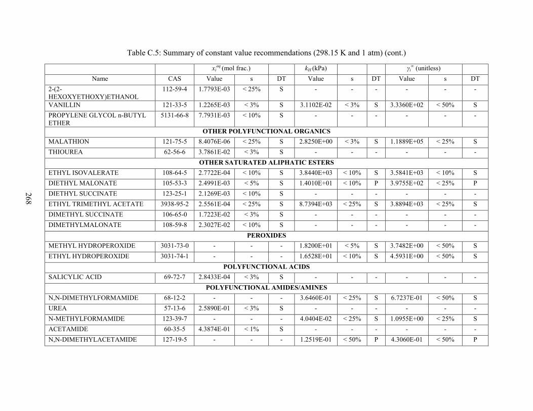
268

Table C.5: Summary of constant value recommendations (298.15 K and 1 atm) (cont.)

xiaq (mol frac.) kH (kPa) γi

∞ (unitless) Name CAS Value s DT Value s DT Value s DT

2-(2-HEXOXYETHOXY)ETHANOL

112-59-4 1.7793E-03 < 25% S - - - - - -

VANILLIN 121-33-5 1.2265E-03 < 3% S 3.1102E-02 < 3% S 3.3360E+02 < 50% S PROPYLENE GLYCOL n-BUTYL ETHER

5131-66-8 7.7931E-03 < 10% S - - - - - -

OTHER POLYFUNCTIONAL ORGANICS MALATHION 121-75-5 8.4076E-06 < 25% S 2.8250E+00 < 3% S 1.1889E+05 < 25% S THIOUREA 62-56-6 3.7861E-02 < 3% S - - - - - -

OTHER SATURATED ALIPHATIC ESTERS ETHYL ISOVALERATE 108-64-5 2.7722E-04 < 10% S 3.8440E+03 < 10% S 3.5841E+03 < 10% S DIETHYL MALONATE 105-53-3 2.4991E-03 < 5% S 1.4010E+01 < 10% P 3.9755E+02 < 25% P DIETHYL SUCCINATE 123-25-1 2.1269E-03 < 10% S - - - - - - ETHYL TRIMETHYL ACETATE 3938-95-2 2.5561E-04 < 25% S 8.7394E+03 < 25% S 3.8894E+03 < 25% S DIMETHYL SUCCINATE 106-65-0 1.7223E-02 < 3% S - - - - - - DIMETHYLMALONATE 108-59-8 2.3027E-02 < 10% S - - - - - -

PEROXIDES METHYL HYDROPEROXIDE 3031-73-0 - - - 1.8200E+01 < 5% S 3.7482E+00 < 50% S ETHYL HYDROPEROXIDE 3031-74-1 - - - 1.6528E+01 < 10% S 4.5931E+00 < 50% S

POLYFUNCTIONAL ACIDS SALICYLIC ACID 69-72-7 2.8433E-04 < 3% S - - - - - -

POLYFUNCTIONAL AMIDES/AMINES N,N-DIMETHYLFORMAMIDE 68-12-2 - - - 3.6460E-01 < 25% S 6.7237E-01 < 50% S UREA 57-13-6 2.5890E-01 < 3% S - - - - - - N-METHYLFORMAMIDE 123-39-7 - - - 4.0404E-02 < 25% S 1.0955E+00 < 25% S ACETAMIDE 60-35-5 4.3874E-01 < 1% S - - - - - - N,N-DIMETHYLACETAMIDE 127-19-5 - - - 1.2519E-01 < 50% P 4.3060E-01 < 50% P

269

Table C.5: Summary of constant value recommendations (298.15 K and 1 atm) (cont.)

xiaq (mol frac.) kH (kPa) γi

∞ (unitless) Name CAS Value s DT Value s DT Value s DT

N,N-DIETHYLHYDROXYLAMINE 3710-84-7 1.0021E-01 < 3% S - - - - - - POLYFUNCTIONAL C, H, N, HALIDE, (O)

o-CHLOROANILINE 95-51-2 1.2271E-03 < 25% S 2.6749E+01 < 25% P 8.0958E+02 < 25% P p-CHLORONITROBENZENE 100-00-5 2.8118E-05 < 10% S 8.6341E+01 < 10% S 2.1744E+04 < 50% S

POLYFUNCTIONAL C, H, O, HALIDE DI(2-CHLOROETHYL)ETHER 111-44-4 1.2915E-03 < 3% S 1.1134E+02 < 3% S 7.7156E+02 < 10% S ETHYLCHLOROACETATE 105-39-5 2.9808E-03 < 5% S 2.1209E+02 < 10% S 3.3591E+02 < 25% S o-CHLOROPHENOL 95-57-8 3.2052E-03 < 3% S - - - - - - m-CHLOROPHENOL 108-43-0 3.2188E-03 < 5% S - - - - - - p-CHLOROPHENOL 106-48-9 3.3222E-03 < 25% S - - - - - - METHYL CHLOROACETATE 96-34-4 8.8232E-03 < 3% S 1.1352E+02 < 3% S 1.1243E+02 < 5% S

POLYFUNCTIONAL C, H, O, N N-METHYL-2-PYRROLIDONE 872-50-4 - - - 1.6824E-02 < 10% S 3.6610E-01 < 10% S ACETAMINOPHEN 103-90-2 1.7020E-03 < 3% S - - - - - - ACETANILIDE 103-84-4 8.1951E-04 < 10% S - - - - - -

POLYFUNCTIONAL C, H, O, S DIMETHYL SULFOXIDE 67-68-5 - - - 6.9311E-03 < 25% S 8.5921E-02 < 25% S

POLYFUNCTIONAL ESTERS METHYL SALICYLATE 119-36-8 1.5371E-04 < 10% S 3.3064E+01 < 25% S 6.4658E+03 < 25% S 2-ETHOXYETHYL ACETATE 111-15-9 3.8954E-02 < 5% S 1.8500E+01 < 10% E ETHYL ACETOACETATE 141-97-9 1.5712E-02 < 25% S 6.1986E+00 < 25% S 6.5389E+01 < 25% S ETHYLENE GLYCOL MONOBUTYL ETHER ACETATE

112-07-2 1.7864E-03 < 25% S 3.0618E+01 < 25% E 2.6500E+02 < 25% D

POLYOLS p-HYDROQUINONE 123-31-9 1.2199E-02 < 3% S - - - - - -

270

Table C.5: Summary of constant value recommendations (298.15 K and 1 atm) (cont.)

xiaq (mol frac.) kH (kPa) γi

∞ (unitless) Name CAS Value s DT Value s DT Value s DT

XYLITOL 87-99-0 1.7785E-01 < 5% S - - - - - - 1,3-BENZENEDIOL 108-46-3 2.1628E-01 < 3% S - - - - - -

PROPIONATES AND BUTYRATES METHYL PROPIONATE 554-12-1 1.2818E-02 < 3% S 9.6262E+02 < 5% S 8.4969E+01 < 5% S ETHYL PROPIONATE 105-37-3 3.4032E-03 < 25% S 1.4323E+03 < 25% S 2.9291E+02 < 25% S n-PROPYL PROPIONATE 106-36-5 9.0986E-04 < 10% S 2.0359E+03 < 10% S 1.0930E+03 < 10% S n-BUTYL PROPIONATE 590-01-2 2.4314E-04 < 5% S 2.4355E+03 < 5% S 4.0803E+03 < 10% S n-PROPYL n-BUTYRATE 105-66-8 2.5274E-04 < 25% S 3.0510E+03 < 25% S 3.9278E+03 < 25% S METHYL n-BUTYRATE 623-42-7 3.0473E-03 < 25% S 1.3329E+03 < 25% S 3.1059E+02 < 25% E ETHYL n-BUTYRATE 105-54-4 1.0223E-03 < 10% S 2.1767E+03 < 10% S 9.7580E+02 < 10% S ISOBUTYL ISOBUTYRATE 97-85-8 7.3381E-05 < 25% S 7.9493E+03 < 25% S 1.3565E+04 < 25% S n-BUTYL n-BUTYRATE 109-21-7 7.9584E-05 < 10% S 3.4019E+03 < 10% S 1.2443E+04 < 10% S METHYL ISOBUTYRATE 547-63-7 3.1917E-03 < 3% S 2.0910E+03 < 10% S 3.1234E+02 < 10% S ETHYL ISOBUTYRATE 97-62-1 9.5920E-04 < 10% S 3.5044E+03 < 10% P 1.0373E+03 < 10% P n-PENTYL n-BUTYRATE 540-18-1 3.1389E-05 < 25% S 3.3166E+03 < 25% S 3.1692E+04 < 25% S ISOPENTYL BUTYRATE 106-27-4 2.7546E-05 < 100% S 5.2634E+03 < 100% S 3.6102E+04 < 100% S

SULFIDES/THIOPHENES DIMETHYL SULFIDE 75-18-3 6.1242E-03 < 10% S 1.0548E+04 < 10% S 1.6343E+02 < 10% S DIMETHYL DISULFIDE 624-92-0 5.6992E-04 < 10% P 6.6448E+03 < 10% S 1.7561E+03 < 10% S 2-METHYLTHIOPHENE 554-14-3 2.4374E-04 < 10% S 1.3663E+04 < 10% S 4.0928E+03 < 10% S DIISOPROPYL SULFIDE 625-80-9 1.3264E-04 < 25% S 1.9586E+04 < 10% S 7.4705E+03 < 25% S

UNSATURATED ALIPHATIC ESTERS ETHYL ACRYLATE 140-88-5 3.5978E-03 < 10% S 1.4139E+03 < 10% P 2.7901E+02 < 10% P METHYL METHACRYLATE 80-62-6 2.7645E-03 < 3% S 1.8891E+03 < 3% S 3.8100E+02 < 10% S DIETHYL MALEATE 141-05-9 1.5787E-03 < 3% S - - - - - -

271

Table C.5: Summary of constant value recommendations (298.15 K and 1 atm) (cont.)

xiaq (mol frac.) kH (kPa) γi

∞ (unitless) Name CAS Value s DT Value s DT Value s DT

DIMETHYL MALEATE 624-48-6 1.0309E-02 < 3% S - - - - - -

273

Appendix D. Experimental Data

Details of each experimental run are included in this appendix. The abbreviations of the

headings are given in Table D.1. Any variables not included in the table are described in Section

5.2.

Table D.1: Abbreviations used in tables with experimental run information

ID Experimental run number ChemID 502 = toluene, 1105 = 1-butanol, 1461 = anisole, 1637 = 1,2-difluorobenzene, 2592 = 1,2,3-

trichlorobenzene, 2661 = 4-bromotoluene, 1579 = 2,4-dichlorotoluene Date Date of experiment Cell Order Experimental number with a given cell Cell T Cell temperature Room T Room temperature Cell P Cell pressure Flow Rate N2 flow rate at room temperature n Number of GC measurements used to calculate the slope, a a Slope (Equation 5.23) sk Error of variable k R2 R2 of plot used to obtain a H2O (g) Water in stripping cell Solute Initial amount of solute; values only included for the first cell run yi max The maximum headspace concentration possible due to the initial amount of solute use Y = run was included when determining final value; N = adsorption effects were significant

so run was not included

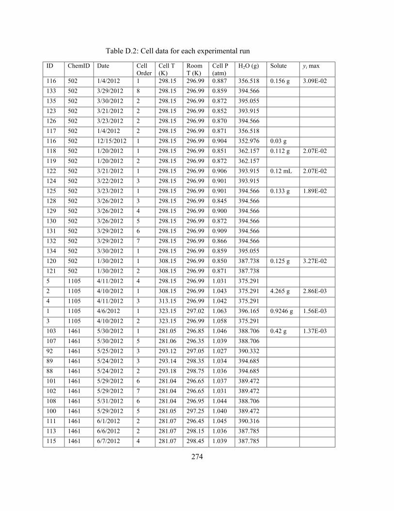
274

Table D.2: Cell data for each experimental run (cont.)

ID ChemID Date Cell Order

Cell T (K)

Room T (K)

Cell P (atm)

H2O (g) Solute yi max

116 502 1/4/2012 1 298.15 296.99 0.887 356.518 0.156 g 3.09E-02 133 502 3/29/2012 8 298.15 296.99 0.859 394.566 135 502 3/30/2012 2 298.15 296.99 0.872 395.055 123 502 3/21/2012 2 298.15 296.99 0.852 393.915 126 502 3/23/2012 2 298.15 296.99 0.870 394.566 117 502 1/4/2012 2 298.15 296.99 0.871 356.518 116 502 12/15/2012 1 298.15 296.99 0.904 352.976 0.03 g 118 502 1/20/2012 1 298.15 296.99 0.851 362.157 0.112 g 2.07E-02 119 502 1/20/2012 2 298.15 296.99 0.872 362.157 122 502 3/21/2012 1 298.15 296.99 0.906 393.915 0.12 mL 2.07E-02 124 502 3/22/2012 3 298.15 296.99 0.901 393.915 125 502 3/23/2012 1 298.15 296.99 0.901 394.566 0.133 g 1.89E-02 128 502 3/26/2012 3 298.15 296.99 0.845 394.566 129 502 3/26/2012 4 298.15 296.99 0.900 394.566 130 502 3/26/2012 5 298.15 296.99 0.872 394.566 131 502 3/29/2012 6 298.15 296.99 0.909 394.566 132 502 3/29/2012 7 298.15 296.99 0.866 394.566 134 502 3/30/2012 1 298.15 296.99 0.859 395.055 120 502 1/30/2012 1 308.15 296.99 0.850 387.738 0.125 g 3.27E-02 121 502 1/30/2012 2 308.15 296.99 0.871 387.738 5 1105 4/11/2012 4 298.15 296.99 1.031 375.291 2 1105 4/10/2012 1 308.15 296.99 1.043 375.291 4.265 g 2.86E-03 4 1105 4/11/2012 3 313.15 296.99 1.042 375.291 1 1105 4/6/2012 1 323.15 297.02 1.063 396.165 0.9246 g 1.56E-03 3 1105 4/10/2012 2 323.15 296.99 1.058 375.291 103 1461 5/30/2012 1 281.05 296.85 1.046 388.706 0.42 g 1.37E-03 107 1461 5/30/2012 5 281.06 296.35 1.039 388.706 92 1461 5/25/2012 3 293.12 297.05 1.027 390.332 89 1461 5/24/2012 3 293.14 298.35 1.034 394.685 88 1461 5/24/2012 2 293.18 298.75 1.036 394.685 101 1461 5/29/2012 6 281.04 296.65 1.037 389.472 102 1461 5/29/2012 7 281.04 296.65 1.031 389.472 108 1461 5/31/2012 6 281.04 296.95 1.044 388.706 100 1461 5/29/2012 5 281.05 297.25 1.040 389.472 111 1461 6/1/2012 2 281.07 296.45 1.045 390.316 113 1461 6/6/2012 2 281.07 298.15 1.036 387.785 115 1461 6/7/2012 4 281.07 298.45 1.039 387.785

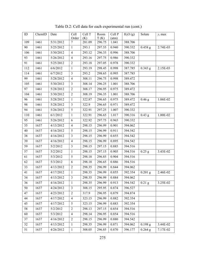
275

Table D.2: Cell data for each experimental run (cont.)

ID ChemID Date Cell Order

Cell T (K)

Room T (K)

Cell P (atm)

H2O (g) Solute yi max

109 1461 5/31/2012 7 281.09 296.75 1.041 388.706 90 1461 5/25/2012 1 293.1 297.55 0.940 390.332 0.458 g 2.74E-03 106 1461 5/30/2012 4 293.12 296.35 0.996 388.706 93 1461 5/26/2012 4 293.16 297.75 0.986 390.332 91 1461 5/25/2012 2 293.18 297.05 0.978 390.332 112 1461 6/6/2012 1 293.19 298.45 0.998 387.785 0.343 g 2.15E-03 114 1461 6/7/2012 3 293.2 298.65 0.995 387.785 99 1461 5/28/2012 4 308.11 296.75 0.998 389.472 105 1461 5/30/2012 3 308.14 296.25 1.001 388.706 97 1461 5/28/2012 2 308.17 296.95 0.975 389.472 104 1461 5/30/2012 2 308.19 296.35 1.001 388.706 96 1461 5/28/2012 1 322.87 296.65 0.975 389.472 0.46 g 1.06E-02 98 1461 5/28/2012 3 322.9 296.65 0.971 389.472 94 1461 5/26/2012 5 322.91 297.25 1.007 390.332 110 1461 6/1/2012 1 322.91 296.65 1.017 390.316 0.43 g 1.00E-02 95 1461 5/26/2012 6 322.92 297.75 0.965 390.332 35 1637 4/13/2012 4 298.15 296.99 0.901 394.062 40 1637 4/16/2012 5 298.15 296.99 0.911 394.542 38 1637 4/16/2012 3 298.15 296.99 0.855 394.542 39 1637 4/16/2012 4 298.15 296.99 0.895 394.542 59 1637 5/2/2012 3 298.15 297.15 0.885 394.516 57 1637 5/2/2012 1 298.15 297.15 0.905 394.516 0.25 g 3.43E-02 61 1637 5/3/2012 5 298.18 296.85 0.904 394.516 62 1637 5/3/2012 6 298.18 296.65 0.886 394.516 33 1637 4/13/2012 2 298.35 296.99 0.844 394.062 41 1637 4/17/2012 1 298.35 296.99 0.855 392.354 0.201 g 2.46E-02 34 1637 4/13/2012 3 298.35 296.99 0.884 394.062 36 1637 4/16/2012 1 298.35 296.99 0.913 394.542 0.21 g 3.25E-02 50 1637 4/24/2012 3 308.15 295.95 0.874 396.527 47 1637 4/23/2012 2 317.9 296.95 0.879 394.874 44 1637 4/17/2012 4 323.15 296.99 0.882 392.354 45 1637 4/17/2012 5 323.15 296.99 0.883 392.354 58 1637 5/2/2012 2 298.13 297.15 0.854 394.516 60 1637 5/3/2012 4 298.14 296.95 0.854 394.516 37 1637 4/16/2012 2 298.15 296.99 0.880 394.542 32 1637 4/13/2012 1 298.35 296.99 0.871 394.062 0.198 g 3.44E-02 51 1637 4/26/2012 1 308.05 296.85 0.870 396.177 0.264 g 7.17E-02

276

Table D.2: Cell data for each experimental run (cont.)

ID ChemID Date Cell Order

Cell T (K)

Room T (K)

Cell P (atm)

H2O (g) Solute yi max

42 1637 4/17/2012 2 308.15 296.99 0.881 392.354 43 1637 4/17/2012 3 308.15 296.99 0.881 392.354 52 1637 4/26/2012 2 317.89 296.65 0.870 396.177 48 1637 4/24/2012 1 317.9 296.15 0.878 396.527 0.243 g 9.01E-02 53 1637 4/27/2012 1 317.92 297.65 0.881 393.315 0.24 g 8.60E-02 54 1637 4/27/2012 2 322.79 297.75 0.881 393.315 2.12E-03 55 1637 4/27/2012 1 322.82 297.65 0.881 393.308 0.25 g 1.08E-01 56 1637 4/27/2012 2 322.83 298.15 0.880 393.308 3.50E-03 46 1637 4/23/2012 1 322.95 296.15 0.882 394.874 0.186 g 8.10E-02 49 1637 4/24/2012 2 323.05 295.65 0.878 396.527 62.5 2592 5/14/2012 293.1 297.15 0.881 394.228 0.002 g 82 2592 6/4/2012 1 281.04 296.45 0.891 394.028 83 2592 6/4/2012 2 281.06 296.45 0.907 394.028 84 2592 6/4/2012 3 281.07 297.05 0.904 394.028 86 2592 6/5/2012 5 281.07 297.15 0.902 394.028 85 2592 6/5/2012 4 281.08 296.25 0.899 394.028 68 2592 5/16/2012 6 292.8 296.35 0.948 395.873 67 2592 5/16/2012 5 292.95 296.25 0.873 395.873 65 2592 5/15/2012 3 293.1 296.65 0.911 395.873 66 2592 5/15/2012 4 293.11 297.35 0.948 395.873 69 2592 5/16/2012 7 293.11 296.15 0.907 395.873 70 2592 5/16/2012 8 293.11 296.25 0.889 395.873 63 2592 5/15/2012 1 293.15 297.15 0.894 395.873 0.002 g 2.85E-05 79 2592 5/23/2012 4 293.21 297.65 0.888 392.05 71 2592 5/16/2012 1 308.1 296.99 0.891 395.47 0.002 g 7.31E-05 72 2592 5/17/2012 2 308.1 296.99 0.837 395.47 73 2592 5/17/2012 3 308.1 296.99 0.837 395.47 81 2592 5/23/2012 6 308.18 297.15 0.887 392.05 80 2592 5/23/2012 5 308.22 297.35 0.889 392.05 74 2592 5/18/2012 4 322.85 296.99 0.898 395.47 75 2592 5/18/2012 5 322.87 296.99 0.898 395.47 76 2592 5/22/2012 1 322.97 296.35 0.896 392.05 0.002 g 1.46E-04 77 2592 5/22/2012 2 322.97 296.35 0.896 392.05 78 2592 5/22/2012 3 322.97 296.05 0.896 392.05 31 2661 5/12/2012 5 293.12 298.15 0.881 395.451 10 2661 5/8/2012 1 308.07 297.15 0.864 394.770 0.020 g 1.04E-03 20 2661 5/11/2012 3 322.9 297.25 0.880 395.451

277

Table D.2: Cell data for each experimental run (cont.)

ID ChemID Date Cell Order

Cell T (K)

Room T (K)

Cell P (atm)

H2O (g) Solute yi max

26 2661 5/10/2012 5 293.07 297.25 0.872 394.844 27 2661 5/10/2012 6 293.09 297.15 0.872 394.844 30 2661 5/11/2012 1 293.15 297.45 0.876 395.451 0.020 g 6.10E-04 29 2661 5/10/2012 9 298.13 296.95 0.872 394.844 28 2661 5/10/2012 7 298.14 297.05 0.873 394.844 25 2661 5/4/2012 1 298.2 297.85 0.874 393.956 0.0005 g 2.41E-05 12 2661 5/8/2012 3 308.05 297.15 0.897 394.770 17 2661 5/9/2012 4 308.07 295.65 0.892 394.844 16 2661 5/9/2012 3 308.08 295.65 0.911 394.844 8 2661 5/7/2012 4 308.093 297.35 0.876 393.956 6 2661 5/7/2012 2 308.1 297.65 0.895 393.956 0.030 g 2.18E-03 9 2661 5/7/2012 5 308.1 295.65 0.912 393.956 13 2661 5/8/2012 4 308.1 296.65 0.878 394.770 15 2661 5/9/2012 2 308.1 296.95 0.877 394.844 21 2661 5/11/2012 4 308.1 297.35 0.876 395.451 7 2661 5/7/2012 3 308.15 297.65 0.861 393.956 11 2661 5/8/2012 2 308.15 297.25 0.916 394.770 14 2661 5/9/2012 1 308.15 297.25 0.862 394.844 0.020 g 1.47E-03 24 2661 5/12/2012 8 317.95 296.75 0.881 395.451 18 2661 5/10/2012 8 318.1 295.75 0.875 394.844 22 2661 5/12/2012 6 322.89 297.05 0.885 395.451 19 2661 5/11/2012 2 322.91 297.65 0.881 395.451 23 2661 5/12/2012 7 322.92 297.05 0.884 395.451 136 1461 8/28/2012 1 280.96 296.35 0.992 386.149 0.420 g 137 1461 8/28/2012 2 280.97 297.15 0.990 386.149 138 1461 8/28/2012 3 280.95 297.15 0.988 386.149 139 1461 8/28/2012 4 280.94 297.35 0.987 386.149 140 1461 8/29/2012 5 280.95 296.85 0.992 386.149 141 2592 8/30/2012 1 293.1 297.35 0.878 394.989 0.002 g 142 2592 8/30/2012 2 293.09 297.15 0.862 394.989 143 2592 8/30/2012 3 323.08 297.15 0.882 394.989 144 2592 8/30/2012 4 323.14 296.95 0.880 394.989 145 2592 8/31/2012 5 323.09 296.95 0.886 394.989 146 2592 8/31/2012 6 308.12 296.95 0.879 394.989 147 2592 8/31/2012 7 280.95 297.05 0.876 394.989 148 2592 9/3/2012 1 293.09 296.95 0.881 393.47 0.002 g 149 2592 9/3/2012 2 280.94 297.15 0.862 393.47

278

Table D.2: Cell data for each experimental run (cont.)

ID ChemID Date Cell Order

Cell T (K)

Room T (K)

Cell P (atm)

H2O (g) Solute yi max

150 2592 9/3/2012 3 280.95 297.25 0.860 393.47 151 2592 9/3/2012 4 280.96 297.25 0.862 393.47 177 1579 9/24/2012 2 323.09 297.25 0.886 395.214 0.013 g 5.38E-03 165 1579 9/10/2012 5 280.91 297.05 0.896 395.521 176 1579 9/24/2012 1 280.95 297.45 0.896 395.214 0.0077 g 1.72E-04 178 1579 9/24/2012 4 280.93 298.05 0.892 395.214 174 1579 9/14/2012 3 280.96 297.95 0.900 394.095 158 1579 9/6/2012 7 293.09 297.25 0.861 395.495 154 1579 9/5/2012 3 293.1 297.15 0.864 395.495 163 1579 9/7/2012 3 293.11 297.55 0.867 395.521 160 1579 9/6/2012 9 293.07 297.15 0.876 395.495 157 1579 9/6/2012 6 293.09 297.15 0.877 395.495 159 1579 9/6/2012 8 293.09 297.15 0.877 395.495 161 1579 9/7/2012 1 293.11 297.25 0.884 395.521 0.0092 g 4.08E-04 173 1579 9/14/2012 2 293.07 298.55 0.903 394.095 155 1579 9/5/2012 4 293.08 297.05 0.896 395.495 153 1579 9/5/2012 2 293.09 297.25 0.898 395.495 162 1579 9/7/2012 2 293.09 297.65 0.901 395.521 156 1579 9/6/2012 5 293.07 296.95 0.912 395.495 152 1579 9/5/2012 1 293.1 297.25 0.916 395.495 0.0092 g 4.95E-04 164 1579 9/7/2012 4 293.12 297.25 0.917 395.521 172 1579 9/14/2012 1 308.14 298.15 0.888 394.095 0.01 g 9.04E-04 168 1579 9/11/2012 1 308.15 297.05 0.898 395.133 169 1579 9/11/2012 2 308.15 297.05 0.897 395.133 166 1579 9/10/2012 6 308.16 296.85 0.896 395.521 171 1579 9/13/2012 4 308.16 298.05 0.906 395.133 178 1579 9/24/2012 3 323.09 297.25 0.867 395.214 175 1579 9/15/2012 4 323.09 296.85 0.890 394.095 0.0123 g 2.98E-03 167 1579 9/10/2012 7 323.09 296.45 0.903 395.521 170 1579 9/13/2012 3 323.14 297.85 0.913 395.133 0.0123 g 3.04E-03

279

Table D.3: Experimental run information—additional parameters (cont.)

ID Flow Rate (mL/min)

n a (1/min) sa R2 use Pisat (Pa) Bii (L/mol) sat

iφ

116 40 8 -2.976E-02 2.47E-04 1.000 N 3803.90 -2.821 0.996 133 12 12 -4.408E-03 8.43E-04 0.646 N 3803.90 -2.821 0.996 135 40 24 -2.204E-02 5.79E-04 0.985 N 3803.90 -2.821 0.996 123 12 18 -3.290E-03 3.49E-04 0.847 N 3803.90 -2.821 0.996 126 40 18 -1.275E-02 2.12E-04 0.996 N 3803.90 -2.821 0.996 117 20.6 10 -1.152E-02 3.25E-04 0.994 Y 3803.90 -2.821 0.996 116 75 5 -4.713E-02 2.66E-04 1.000 Y 3803.90 -2.821 0.996 118 12 24 -8.416E-03 7.31E-05 0.998 Y 3803.90 -2.821 0.996 119 40 21 -3.023E-02 2.39E-04 0.999 Y 3803.90 -2.821 0.996 122 75 19 -4.995E-02 4.31E-04 0.999 Y 3803.90 -2.821 0.996 124 75 12 -5.176E-02 2.93E-04 1.000 Y 3803.90 -2.821 0.996 125 75 12 -4.140E-02 3.75E-04 0.999 Y 3803.90 -2.821 0.996 128 12 25 -7.072E-03 1.43E-04 0.991 Y 3803.90 -2.821 0.996 129 75 12 -5.308E-02 2.28E-04 1.000 Y 3803.90 -2.821 0.996 130 40 9 -2.786E-02 4.30E-04 0.998 Y 3803.90 -2.821 0.996 131 75 14 -5.389E-02 1.77E-04 1.000 Y 3803.90 -2.821 0.996 132 40 8 -2.583E-02 7.31E-04 0.995 Y 3803.90 -2.821 0.996 134 12 31 -6.215E-03 2.57E-04 0.953 Y 3803.90 -2.821 0.996 120 12 21 -1.243E-02 8.79E-05 0.999 Y 6239.14 -2.509 0.994 121 40 8 -4.443E-02 1.04E-03 0.997 Y 6239.14 -2.509 0.994 5 200 21 -2.784E-04 2.18E-05 0.896 Y 900.84 -10.036 0.996 2 200 27 -4.328E-04 1.64E-05 0.965 Y 1797.89 -7.800 0.995 4 200 21 -5.840E-04 2.35E-05 0.970 Y 2487.26 -6.906 0.993 1 200 29 -1.163E-03 4.84E-05 0.955 Y 4580.99 -5.459 0.991 3 200 21 -1.063E-03 2.03E-05 0.993 Y 4580.99 -5.459 0.991 103 200 19 -2.935E-03 4.40E-04 0.723 N 150.11 0.000 1.000 107 200 14 -2.095E-03 3.85E-04 0.712 N 150.22 0.000 1.000 92 200 19 -4.867E-03 1.43E-04 0.986 N 348.35 0.000 1.000 89 200 24 -4.429E-03 1.73E-04 0.967 N 348.81 0.000 1.000 88 200 20 -4.693E-03 1.54E-04 0.981 N 349.74 0.000 1.000 101 200 14 -3.084E-03 3.63E-05 0.998 N 150.00 0.000 1.000 102 200 13 -2.576E-03 1.63E-04 0.958 N 150.00 0.000 1.000 108 200 21 -2.468E-03 1.32E-04 0.949 N 150.00 0.000 1.000 100 200 16 -3.128E-03 3.74E-04 0.833 N 150.11 0.000 1.000 111 200 44 -2.334E-03 6.83E-05 0.965 N 150.33 0.000 1.000 113 200 29 -2.378E-03 4.36E-05 0.991 N 150.33 0.000 1.000 115 200 24 -2.350E-03 3.33E-05 0.996 N 150.33 0.000 1.000

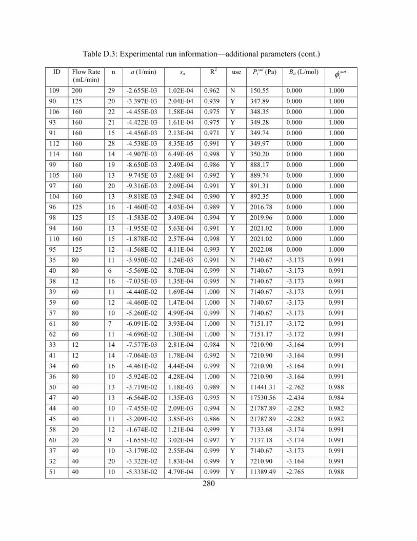
280

Table D.3: Experimental run information—additional parameters (cont.)

ID Flow Rate (mL/min)

n a (1/min) sa R2 use Pisat (Pa) Bii (L/mol) sat

iφ

109 200 29 -2.655E-03 1.02E-04 0.962 N 150.55 0.000 1.000 90 125 20 -3.397E-03 2.04E-04 0.939 Y 347.89 0.000 1.000 106 160 22 -4.455E-03 1.58E-04 0.975 Y 348.35 0.000 1.000 93 160 21 -4.422E-03 1.61E-04 0.975 Y 349.28 0.000 1.000 91 160 15 -4.456E-03 2.13E-04 0.971 Y 349.74 0.000 1.000 112 160 28 -4.538E-03 8.35E-05 0.991 Y 349.97 0.000 1.000 114 160 14 -4.907E-03 6.49E-05 0.998 Y 350.20 0.000 1.000 99 160 19 -8.650E-03 2.49E-04 0.986 Y 888.17 0.000 1.000 105 160 13 -9.745E-03 2.68E-04 0.992 Y 889.74 0.000 1.000 97 160 20 -9.316E-03 2.09E-04 0.991 Y 891.31 0.000 1.000 104 160 13 -9.818E-03 2.94E-04 0.990 Y 892.35 0.000 1.000 96 125 16 -1.460E-02 4.03E-04 0.989 Y 2016.78 0.000 1.000 98 125 15 -1.583E-02 3.49E-04 0.994 Y 2019.96 0.000 1.000 94 160 13 -1.955E-02 5.63E-04 0.991 Y 2021.02 0.000 1.000 110 160 15 -1.878E-02 2.57E-04 0.998 Y 2021.02 0.000 1.000 95 125 12 -1.568E-02 4.11E-04 0.993 Y 2022.08 0.000 1.000 35 80 11 -3.950E-02 1.24E-03 0.991 N 7140.67 -3.173 0.991 40 80 6 -5.569E-02 8.70E-04 0.999 N 7140.67 -3.173 0.991 38 12 16 -7.035E-03 1.35E-04 0.995 N 7140.67 -3.173 0.991 39 60 11 -4.440E-02 1.69E-04 1.000 N 7140.67 -3.173 0.991 59 60 12 -4.460E-02 1.47E-04 1.000 N 7140.67 -3.173 0.991 57 80 10 -5.260E-02 4.99E-04 0.999 N 7140.67 -3.173 0.991 61 80 7 -6.091E-02 3.93E-04 1.000 N 7151.17 -3.172 0.991 62 60 11 -4.696E-02 1.30E-04 1.000 N 7151.17 -3.172 0.991 33 12 14 -7.577E-03 2.81E-04 0.984 N 7210.90 -3.164 0.991 41 12 14 -7.064E-03 1.78E-04 0.992 N 7210.90 -3.164 0.991 34 60 16 -4.461E-02 4.44E-04 0.999 N 7210.90 -3.164 0.991 36 80 10 -5.924E-02 4.28E-04 1.000 N 7210.90 -3.164 0.991 50 40 13 -3.719E-02 1.18E-03 0.989 N 11441.31 -2.762 0.988 47 40 13 -6.564E-02 1.35E-03 0.995 N 17530.56 -2.434 0.984 44 40 10 -7.455E-02 2.09E-03 0.994 N 21787.89 -2.282 0.982 45 40 11 -3.209E-02 3.85E-03 0.886 N 21787.89 -2.282 0.982 58 20 12 -1.674E-02 1.21E-04 0.999 Y 7133.68 -3.174 0.991 60 20 9 -1.655E-02 3.02E-04 0.997 Y 7137.18 -3.174 0.991 37 40 10 -3.179E-02 2.55E-04 0.999 Y 7140.67 -3.173 0.991 32 40 20 -3.322E-02 1.83E-04 0.999 Y 7210.90 -3.164 0.991 51 40 10 -5.333E-02 4.79E-04 0.999 Y 11389.49 -2.765 0.988

281

Table D.3: Experimental run information—additional parameters (cont.)

ID Flow Rate (mL/min)

n a (1/min) sa R2 use Pisat (Pa) Bii (L/mol) sat

iφ

42 40 11 -5.131E-02 3.25E-04 1.000 Y 11441.31 -2.762 0.988 43 40 11 -4.992E-02 4.92E-04 0.999 Y 11441.31 -2.762 0.988 52 40 10 -7.685E-02 5.57E-04 1.000 Y 17523.17 -2.434 0.984 48 40 10 -7.620E-02 6.40E-04 0.999 Y 17530.56 -2.434 0.984 53 40 8 -7.298E-02 6.26E-04 1.000 Y 17545.37 -2.433 0.984 54 40 7 -7.877E-02 1.20E-03 0.999 Y 21471.13 -2.292 0.982 55 40 10 -9.078E-02 7.59E-04 0.999 Y 21497.39 -2.291 0.982 56 40 10 -8.442E-02 1.29E-03 0.998 Y 21506.14 -2.291 0.982 46 40 11 -9.225E-02 7.88E-04 0.999 Y 21611.45 -2.288 0.982 49 40 7 -9.020E-02 1.10E-03 0.999 Y 21699.52 -2.285 0.982 62.5 40 12 -4.826E-03 6.46E-04 0.848 N 11.25 0.000 1.000 82 60 30 -2.853E-03 9.86E-05 0.968 Y 3.43 0.000 1.000 83 80 29 -3.674E-03 1.01E-04 0.980 Y 3.44 0.000 1.000 84 80 27 -3.503E-03 2.07E-04 0.919 Y 3.44 0.000 1.000 86 80 29 -3.857E-03 6.77E-05 0.992 Y 3.44 0.000 1.000 85 80 27 -3.613E-03 1.13E-04 0.976 Y 3.45 0.000 1.000 68 120 13 -1.082E-02 2.77E-04 0.993 Y 10.93 0.000 1.000 67 40 16 -5.050E-03 1.72E-04 0.984 Y 11.09 0.000 1.000 65 80 16 -8.354E-03 1.99E-04 0.992 Y 11.25 0.000 1.000 66 120 13 -1.215E-02 3.03E-04 0.993 Y 11.26 0.000 1.000 69 80 16 -8.347E-03 2.47E-04 0.988 Y 11.26 0.000 1.000 70 60 8 -5.120E-03 1.48E-04 0.995 Y 11.26 0.000 1.000 63 60 13 -6.519E-03 2.01E-04 0.990 Y 11.30 0.000 1.000 79 60 17 -6.887E-03 2.21E-04 0.985 Y 11.36 0.000 1.000 71 60 27 -1.734E-02 7.29E-05 1.000 Y 43.19 0.000 1.000 72 60 16 -1.714E-02 1.85E-04 0.998 Y 43.19 0.000 1.000 73 60 12 -1.528E-02 3.97E-04 0.993 Y 43.19 0.000 1.000 81 60 12 -1.692E-02 3.14E-04 0.997 Y 43.49 0.000 1.000 80 60 14 -1.826E-02 3.21E-04 0.996 Y 43.64 0.000 1.000 74 60 20 -3.492E-02 1.84E-04 1.000 Y 143.60 0.000 1.000 75 60 11 -3.028E-02 3.34E-04 0.999 Y 143.83 0.000 1.000 76 60 10 -3.748E-02 5.15E-04 0.998 Y 144.95 0.000 1.000 77 60 10 -3.525E-02 1.31E-03 0.989 Y 144.95 0.000 1.000 78 60 10 -3.076E-02 8.36E-04 0.994 Y 144.95 0.000 1.000 31 40 9 -8.788E-03 3.25E-04 0.990 N 113.95 0.000 1.000 10 20 13 -7.729E-03 3.94E-04 0.972 N 331.94 0.000 1.000 20 40 12 -4.311E-02 6.95E-04 0.997 N 755.72 0.000 1.000

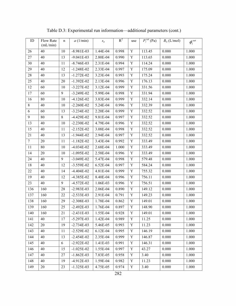
282

Table D.3: Experimental run information—additional parameters (cont.)

ID Flow Rate (mL/min)

n a (1/min) sa R2 use Pisat (Pa) Bii (L/mol) sat

iφ

26 40 10 -8.981E-03 1.44E-04 0.998 Y 113.45 0.000 1.000 27 40 13 -9.041E-03 2.80E-04 0.990 Y 113.65 0.000 1.000 30 40 11 -8.746E-03 2.31E-04 0.994 Y 114.24 0.000 1.000 29 40 12 -1.248E-02 2.33E-04 0.997 Y 175.09 0.000 1.000 28 40 13 -1.272E-02 3.23E-04 0.993 Y 175.24 0.000 1.000 25 40 20 -1.392E-02 2.13E-04 0.996 Y 176.13 0.000 1.000 12 60 10 -3.227E-02 3.12E-04 0.999 Y 331.56 0.000 1.000 17 60 9 -3.249E-02 5.99E-04 0.998 Y 331.94 0.000 1.000 16 80 10 -4.126E-02 3.83E-04 0.999 Y 332.14 0.000 1.000 8 40 10 -2.260E-02 5.24E-04 0.996 Y 332.39 0.000 1.000 6 60 13 -3.234E-02 2.20E-04 0.999 Y 332.52 0.000 1.000 9 80 8 -4.429E-02 9.81E-04 0.997 Y 332.52 0.000 1.000 13 40 10 -2.230E-02 4.79E-04 0.996 Y 332.52 0.000 1.000 15 40 11 -2.152E-02 3.08E-04 0.998 Y 332.52 0.000 1.000 21 40 13 -1.944E-02 2.94E-04 0.997 Y 332.52 0.000 1.000 7 20 11 -1.182E-02 3.43E-04 0.992 Y 333.49 0.000 1.000 11 80 10 -4.034E-02 2.68E-04 1.000 Y 333.49 0.000 1.000 14 20 10 -1.095E-02 2.58E-04 0.996 Y 333.49 0.000 1.000 24 40 9 -3.049E-02 5.47E-04 0.998 Y 579.48 0.000 1.000 18 40 12 -3.559E-02 6.52E-04 0.997 Y 584.24 0.000 1.000 22 40 14 -4.404E-02 4.81E-04 0.999 Y 755.32 0.000 1.000 19 40 12 -4.385E-02 8.40E-04 0.996 Y 756.11 0.000 1.000 23 40 9 -4.572E-02 1.06E-03 0.996 Y 756.51 0.000 1.000 136 160 28 -2.983E-03 2.06E-04 0.890 Y 149.12 0.000 1.000 137 160 22 -2.533E-03 2.91E-04 0.791 Y 149.23 0.000 1.000 138 160 29 -2.308E-03 1.78E-04 0.862 Y 149.01 0.000 1.000 139 160 25 -2.492E-03 1.76E-04 0.897 Y 148.90 0.000 1.000 140 160 21 -2.431E-03 1.55E-04 0.928 Y 149.01 0.000 1.000 141 40 17 -5.297E-03 1.42E-04 0.989 Y 11.25 0.000 1.000 142 20 19 -2.734E-03 5.46E-05 0.993 Y 11.23 0.000 1.000 143 40 11 -2.529E-02 6.12E-04 0.995 Y 146.19 0.000 1.000 144 40 13 -2.454E-02 2.35E-04 0.999 Y 146.87 0.000 1.000 145 40 6 -2.922E-02 1.41E-03 0.991 Y 146.31 0.000 1.000 146 40 15 -1.025E-02 1.55E-04 0.997 Y 43.27 0.000 1.000 147 40 27 -1.862E-03 7.83E-05 0.958 Y 3.40 0.000 1.000 148 40 19 -4.912E-03 1.59E-04 0.982 Y 11.23 0.000 1.000 149 20 23 -1.325E-03 4.75E-05 0.974 Y 3.40 0.000 1.000

283

Table D.3: Experimental run information—additional parameters (cont.)

ID Flow Rate (mL/min)

n a (1/min) sa R2 use Pisat (Pa) Bii (L/mol) sat

iφ

150 20 22 -1.319E-03 5.88E-05 0.962 Y 3.40 0.000 1.000 151 20 21 -1.127E-03 6.26E-05 0.947 Y 3.41 0.000 1.000 177 40 5 -1.223E-01 1.29E-02 0.968 N 312.47 0.000 1.000 165 60 17 -9.249E-03 1.87E-04 0.994 Y 16.21 0.000 1.000 176 60 18 -8.918E-03 2.70E-04 0.986 Y 16.27 0.000 1.000 178 60 23 -8.111E-03 1.89E-04 0.989 Y 16.24 0.000 1.000 174 60 29 -5.586E-03 1.27E-04 0.986 Y 16.28 0.000 1.000 158 20 21 -6.145E-03 1.79E-04 0.984 Y 42.14 0.000 1.000 154 20 19 -7.578E-03 1.83E-04 0.990 Y 42.17 0.000 1.000 163 20 17 -4.762E-03 2.01E-04 0.974 Y 42.21 0.000 1.000 160 40 12 -1.257E-02 4.26E-04 0.989 Y 42.08 0.000 1.000 157 40 15 -1.141E-02 2.50E-04 0.994 Y 42.14 0.000 1.000 159 40 9 -1.426E-02 3.49E-04 0.996 Y 42.14 0.000 1.000 161 40 11 -1.197E-02 2.98E-04 0.994 Y 42.21 0.000 1.000 173 60 8 -1.530E-02 3.84E-04 0.996 Y 42.08 0.000 1.000 155 60 9 -2.187E-02 1.09E-03 0.983 Y 42.11 0.000 1.000 153 60 12 -2.201E-02 2.30E-04 0.999 Y 42.14 0.000 1.000 162 60 11 -1.915E-02 4.05E-04 0.996 Y 42.14 0.000 1.000 156 80 13 -2.657E-02 2.49E-04 0.999 Y 42.08 0.000 1.000 152 80 12 -2.897E-02 3.54E-04 0.999 Y 42.17 0.000 1.000 164 80 12 -1.974E-02 2.16E-04 0.999 Y 42.24 0.000 1.000 172 40 12 -2.513E-02 2.43E-04 0.999 Y 121.81 0.000 1.000 168 60 9 -2.597E-02 2.21E-04 0.999 Y 121.89 0.000 1.000 169 60 6 -3.236E-02 8.08E-04 0.998 Y 121.89 0.000 1.000 166 60 7 -4.541E-02 6.52E-04 0.999 Y 121.97 0.000 1.000 171 60 6 -4.801E-02 1.18E-03 0.998 Y 121.97 0.000 1.000 178 20 7 -2.992E-02 1.08E-03 0.994 Y 312.47 0.000 1.000 175 40 7 -7.261E-02 9.32E-04 0.999 Y 312.47 0.000 1.000 167 60 6 -7.037E-02 3.04E-03 0.993 Y 312.47 0.000 1.000 170 60 5 -1.106E-01 3.08E-03 0.998 Y 313.40 0.000 1.000

284

Table D.4: Experimental run calculated values (cont.)

ID Ψ sΨ γi∞ sγ∞ (%) kH

(kPa∙mol/mol) skH (%)

116 1 0 9.65E+03 5.2% 3.66E+04 7.9% 133 1 0 5.09E+03 5.2% 1.93E+04 19.3% 135 1 0 7.67E+03 5.2% 2.90E+04 8.0% 123 1 0 3.78E+03 5.2% 1.43E+04 10.8% 126 1 0 4.41E+03 5.2% 1.67E+04 7.7% 117 1 0 7.18E+03 5.2% 2.72E+04 15.3% 116 1 0 8.04E+03 5.2% 3.05E+04 4.2% 118 1 0 9.17E+03 5.2% 3.47E+04 2.0% 119 1 0 9.92E+03 5.2% 3.76E+04 7.8% 122 1 0 9.28E+03 5.2% 3.52E+04 4.2% 124 1 0 9.62E+03 5.2% 3.64E+04 4.1% 125 1 0 7.69E+03 5.2% 2.91E+04 4.2% 128 1 0 8.19E+03 5.2% 3.10E+04 2.6% 129 1 0 9.88E+03 5.2% 3.74E+04 4.1% 130 1 0 9.71E+03 5.2% 3.68E+04 7.8% 131 1 0 1.00E+04 5.2% 3.80E+04 4.1% 132 1 0 8.99E+03 5.2% 3.41E+04 8.1% 134 1 0 7.20E+03 5.2% 2.73E+04 4.5% 120 1 0 8.49E+03 5.2% 5.26E+04 2.0% 121 1 0 9.13E+03 5.2% 5.66E+04 7.9%

5 1 0 7.74E+01 25.3% 6.94E+01 8.0% 2 1 0 5.89E+01 25.2% 1.05E+02 4.1% 4 1 0 5.65E+01 25.2% 1.40E+02 4.3% 1 1 0 6.16E+01 25.1% 2.80E+02 4.4% 3 1 0 5.33E+01 25.1% 2.42E+02 2.4%

103 1 0 5.16E+03 25.4% 7.74E+02 15.1% 107 1 0 3.67E+03 25.4% 5.51E+02 18.4% 92 1 0 3.66E+03 25.4% 1.27E+03 3.3% 89 1 0 3.37E+03 25.4% 1.18E+03 4.2% 88 1 0 3.57E+03 25.4% 1.25E+03 3.6%

101 1 0 5.43E+03 25.4% 8.14E+02 2.0% 102 1 0 4.53E+03 25.4% 6.80E+02 6.5% 108 1 0 4.34E+03 25.4% 6.51E+02 5.6% 100 1 0 5.51E+03 25.4% 8.28E+02 12.1% 111 1 0 4.10E+03 25.4% 6.17E+02 3.3% 113 1 0 4.18E+03 25.4% 6.28E+02 2.4%

285

Table D.4: Experimental run calculated values (cont.)

ID Ψ sΨ γi∞ sγ∞ (%) kH

(kPa∙mol/mol) skH (%)

115 1 0 4.13E+03 25.4% 6.21E+02 2.1% 109 1 0 4.65E+03 25.4% 7.00E+02 4.1% 90 1 0 4.09E+03 25.4% 1.42E+03 6.5%

106 1 0 4.15E+03 25.4% 1.45E+03 4.0% 93 1 0 4.15E+03 25.4% 1.45E+03 4.1% 91 1 0 4.16E+03 25.4% 1.46E+03 5.1%

112 1 0 4.23E+03 25.4% 1.48E+03 2.7% 114 1 0 4.58E+03 25.4% 1.60E+03 2.3% 99 1 0 3.07E+03 25.4% 2.73E+03 3.4%

105 1 0 3.44E+03 25.4% 3.06E+03 3.3% 97 1 0 3.29E+03 25.4% 2.93E+03 2.9%

104 1 0 3.46E+03 25.4% 3.08E+03 3.5% 96 1 0 2.71E+03 25.4% 5.47E+03 3.5% 98 1 0 2.93E+03 25.4% 5.93E+03 3.1% 94 1 0 2.86E+03 25.4% 5.77E+03 3.4%

110 1 0 2.74E+03 25.4% 5.54E+03 2.2% 95 1 0 2.92E+03 25.4% 5.90E+03 3.4% 35 1 0 3.67E+03 10.0% 2.60E+04 5.0% 40 1 0 5.20E+03 10.0% 3.68E+04 4.2% 38 1 0 4.36E+03 10.0% 3.09E+04 2.5% 39 1 0 5.53E+03 10.0% 3.91E+04 5.1% 59 1 0 5.56E+03 10.0% 3.93E+04 5.1% 57 1 0 4.91E+03 10.0% 3.48E+04 4.0% 61 1 0 5.68E+03 10.0% 4.03E+04 3.9% 62 1 0 5.84E+03 10.0% 4.14E+04 5.1% 33 1 0 4.65E+03 10.0% 3.32E+04 4.1% 41 1 0 4.32E+03 10.0% 3.08E+04 3.0% 34 1 0 5.49E+03 10.0% 3.93E+04 5.2% 36 1 0 5.48E+03 10.0% 3.92E+04 3.9% 50 1 0 4.23E+03 10.0% 4.78E+04 8.0% 47 1 0 4.70E+03 9.9% 8.11E+04 7.6% 44 1 0 4.14E+03 9.9% 8.86E+04 7.8% 45 1 0 1.76E+03 9.9% 3.76E+04 14.0% 58 1 0 6.26E+03 10.0% 4.43E+04 15.2% 60 1 0 6.19E+03 10.0% 4.38E+04 15.3% 37 1 0 5.94E+03 10.0% 4.20E+04 7.7%

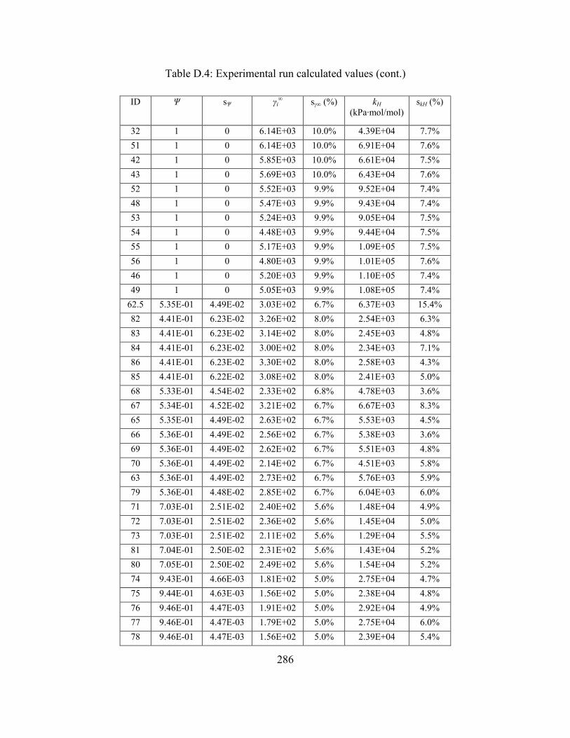
286

Table D.4: Experimental run calculated values (cont.)

ID Ψ sΨ γi∞ sγ∞ (%) kH

(kPa∙mol/mol) skH (%)

32 1 0 6.14E+03 10.0% 4.39E+04 7.7% 51 1 0 6.14E+03 10.0% 6.91E+04 7.6% 42 1 0 5.85E+03 10.0% 6.61E+04 7.5% 43 1 0 5.69E+03 10.0% 6.43E+04 7.6% 52 1 0 5.52E+03 9.9% 9.52E+04 7.4% 48 1 0 5.47E+03 9.9% 9.43E+04 7.4% 53 1 0 5.24E+03 9.9% 9.05E+04 7.5% 54 1 0 4.48E+03 9.9% 9.44E+04 7.5% 55 1 0 5.17E+03 9.9% 1.09E+05 7.5% 56 1 0 4.80E+03 9.9% 1.01E+05 7.6% 46 1 0 5.20E+03 9.9% 1.10E+05 7.4% 49 1 0 5.05E+03 9.9% 1.08E+05 7.4%

62.5 5.35E-01 4.49E-02 3.03E+02 6.7% 6.37E+03 15.4% 82 4.41E-01 6.23E-02 3.26E+02 8.0% 2.54E+03 6.3% 83 4.41E-01 6.23E-02 3.14E+02 8.0% 2.45E+03 4.8% 84 4.41E-01 6.23E-02 3.00E+02 8.0% 2.34E+03 7.1% 86 4.41E-01 6.23E-02 3.30E+02 8.0% 2.58E+03 4.3% 85 4.41E-01 6.22E-02 3.08E+02 8.0% 2.41E+03 5.0% 68 5.33E-01 4.54E-02 2.33E+02 6.8% 4.78E+03 3.6% 67 5.34E-01 4.52E-02 3.21E+02 6.7% 6.67E+03 8.3% 65 5.35E-01 4.49E-02 2.63E+02 6.7% 5.53E+03 4.5% 66 5.36E-01 4.49E-02 2.56E+02 6.7% 5.38E+03 3.6% 69 5.36E-01 4.49E-02 2.62E+02 6.7% 5.51E+03 4.8% 70 5.36E-01 4.49E-02 2.14E+02 6.7% 4.51E+03 5.8% 63 5.36E-01 4.49E-02 2.73E+02 6.7% 5.76E+03 5.9% 79 5.36E-01 4.48E-02 2.85E+02 6.7% 6.04E+03 6.0% 71 7.03E-01 2.51E-02 2.40E+02 5.6% 1.48E+04 4.9% 72 7.03E-01 2.51E-02 2.36E+02 5.6% 1.45E+04 5.0% 73 7.03E-01 2.51E-02 2.11E+02 5.6% 1.29E+04 5.5% 81 7.04E-01 2.50E-02 2.31E+02 5.6% 1.43E+04 5.2% 80 7.05E-01 2.50E-02 2.49E+02 5.6% 1.54E+04 5.2% 74 9.43E-01 4.66E-03 1.81E+02 5.0% 2.75E+04 4.7% 75 9.44E-01 4.63E-03 1.56E+02 5.0% 2.38E+04 4.8% 76 9.46E-01 4.47E-03 1.91E+02 5.0% 2.92E+04 4.9% 77 9.46E-01 4.47E-03 1.79E+02 5.0% 2.75E+04 6.0% 78 9.46E-01 4.47E-03 1.56E+02 5.0% 2.39E+04 5.4%

287

Table D.4: Experimental run calculated values (cont.)

ID Ψ sΨ γi∞ sγ∞ (%) kH

(kPa∙mol/mol) skH (%)

31 8.70E-01 0.05172 8.93E+01 25.5% 1.17E+04 8.5% 10 1 0 5.93E+04 10.9% 1.97E+04 15.4% 20 1 0 6.76E+04 10.9% 5.11E+04 7.2% 26 8.69E-01 0.052071 9.11E+01 25.5% 1.19E+04 7.8% 27 8.70E-01 0.051931 9.16E+01 25.5% 1.20E+04 8.2% 30 8.71E-01 0.051509 8.84E+01 25.5% 1.16E+04 8.1% 29 9.64E-01 0.014676 9.02E+01 25.0% 1.64E+04 7.8% 28 9.64E-01 0.014598 9.19E+01 25.0% 1.67E+04 7.9% 25 9.66E-01 0.014126 1.00E+02 25.0% 1.83E+04 7.7% 12 1 0 8.31E+04 10.9% 2.76E+04 5.0% 17 1 0 8.31E+04 10.9% 2.76E+04 5.2% 16 1 0 7.92E+04 10.9% 2.63E+04 3.8% 8 1 0 8.69E+04 10.9% 2.89E+04 7.7% 6 1 0 8.30E+04 10.9% 2.76E+04 5.0% 9 1 0 8.48E+04 10.9% 2.82E+04 4.3%

13 1 0 8.56E+04 10.9% 2.85E+04 7.6% 15 1 0 8.27E+04 10.9% 2.75E+04 7.5% 21 1 0 7.48E+04 10.9% 2.49E+04 7.5% 7 1 0 9.06E+04 10.9% 3.02E+04 14.9%

11 1 0 7.75E+04 10.9% 2.59E+04 3.7% 14 1 0 8.39E+04 10.9% 2.80E+04 14.8% 24 1 0 6.43E+04 10.9% 3.73E+04 7.3% 18 1 0 7.41E+04 10.9% 4.33E+04 7.3% 22 1 0 6.91E+04 10.9% 5.22E+04 7.1% 19 1 0 6.88E+04 10.9% 5.21E+04 7.3% 23 1 0 7.17E+04 10.9% 5.42E+04 7.5%

136 1 0 6.54E+03 10.9% 9.75E+02 7.2% 137 1 0 5.56E+03 10.9% 8.30E+02 11.7% 138 1 0 5.07E+03 10.9% 7.56E+02 8.0% 139 1 0 5.49E+03 10.9% 8.17E+02 7.3% 140 1 0 5.34E+03 10.9% 7.96E+02 6.7% 141 5.35E-01 4.49E-02 3.34E+02 6.7% 7.01E+03 8.1% 142 5.35E-01 4.50E-02 3.44E+02 6.7% 7.23E+03 15.4% 143 9.48E-01 4.29E-03 1.93E+02 5.0% 2.97E+04 7.4% 144 9.49E-01 4.20E-03 1.86E+02 5.0% 2.88E+04 7.0% 145 9.48E-01 4.28E-03 2.23E+02 5.0% 3.44E+04 8.5%

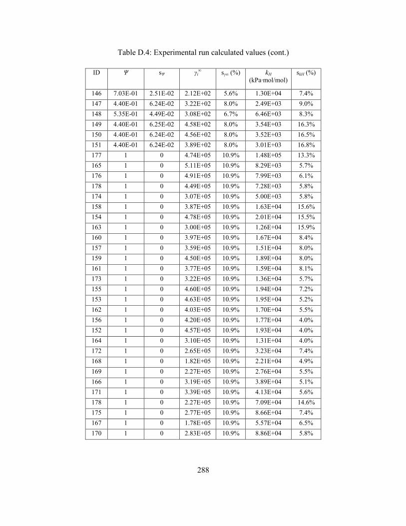
288

Table D.4: Experimental run calculated values (cont.)

ID Ψ sΨ γi∞ sγ∞ (%) kH

(kPa∙mol/mol) skH (%)

146 7.03E-01 2.51E-02 2.12E+02 5.6% 1.30E+04 7.4% 147 4.40E-01 6.24E-02 3.22E+02 8.0% 2.49E+03 9.0% 148 5.35E-01 4.49E-02 3.08E+02 6.7% 6.46E+03 8.3% 149 4.40E-01 6.25E-02 4.58E+02 8.0% 3.54E+03 16.3% 150 4.40E-01 6.24E-02 4.56E+02 8.0% 3.52E+03 16.5% 151 4.40E-01 6.24E-02 3.89E+02 8.0% 3.01E+03 16.8% 177 1 0 4.74E+05 10.9% 1.48E+05 13.3% 165 1 0 5.11E+05 10.9% 8.29E+03 5.7% 176 1 0 4.91E+05 10.9% 7.99E+03 6.1% 178 1 0 4.49E+05 10.9% 7.28E+03 5.8% 174 1 0 3.07E+05 10.9% 5.00E+03 5.8% 158 1 0 3.87E+05 10.9% 1.63E+04 15.6% 154 1 0 4.78E+05 10.9% 2.01E+04 15.5% 163 1 0 3.00E+05 10.9% 1.26E+04 15.9% 160 1 0 3.97E+05 10.9% 1.67E+04 8.4% 157 1 0 3.59E+05 10.9% 1.51E+04 8.0% 159 1 0 4.50E+05 10.9% 1.89E+04 8.0% 161 1 0 3.77E+05 10.9% 1.59E+04 8.1% 173 1 0 3.22E+05 10.9% 1.36E+04 5.7% 155 1 0 4.60E+05 10.9% 1.94E+04 7.2% 153 1 0 4.63E+05 10.9% 1.95E+04 5.2% 162 1 0 4.03E+05 10.9% 1.70E+04 5.5% 156 1 0 4.20E+05 10.9% 1.77E+04 4.0% 152 1 0 4.57E+05 10.9% 1.93E+04 4.0% 164 1 0 3.10E+05 10.9% 1.31E+04 4.0% 172 1 0 2.65E+05 10.9% 3.23E+04 7.4% 168 1 0 1.82E+05 10.9% 2.21E+04 4.9% 169 1 0 2.27E+05 10.9% 2.76E+04 5.5% 166 1 0 3.19E+05 10.9% 3.89E+04 5.1% 171 1 0 3.39E+05 10.9% 4.13E+04 5.6% 178 1 0 2.27E+05 10.9% 7.09E+04 14.6% 175 1 0 2.77E+05 10.9% 8.66E+04 7.4% 167 1 0 1.78E+05 10.9% 5.57E+04 6.5% 170 1 0 2.83E+05 10.9% 8.86E+04 5.8%

289

Appendix E. Prediction Method Sample Calculations

E.1 First-Order Group Contribution Method

E.1.1. 1,2,4,5-Tetramethylbenzene

Structural information and group contributions:

Group ni∙ ∞∆ ihydG , (kJ/mol) ni∙Bi (K) ni∙Ci

CH3 4∙(3.67) 4∙3683 4∙(-8.73) CHar 2∙(-0.65) 2∙1849 2∙(-4.16) Car 4∙(-3.85) 4∙(-102) 4∙(0.05) I(C-C) 2∙(-1.01) 2∙6047 2∙(-19.2) Y0 7.95 0 0 Total 3.91 30116 -81.44

Equation 7.2 is rearranged to solve for kH,ref:

molmolkPa10723.2

K15.298Kmol

J3145.8

molJ100091.3

expmolmol5084.55kPa325.101 4

, ⋅⋅=

⋅⋅⋅

⋅⋅⋅⋅=refHk .

The overall temperature-dependent equation for kH is predicted by:

( ) ( ) ( )

⋅⋅+

⋅−+

−

⋅⋅=

molmolkPa10723.2ln

K15.298ln44.811

K15.2981K30116ln 4T

TkH .

290

E.1.2. 2,2-Dimethylhexane

Structural information and group contributions:

Group ni∙ ∞∆ ihydG , (kJ/mol) ni∙Bi (K) ni∙Ci

CH3 4∙(3.67) 4∙3683 4∙(-8.73) CH2 3∙(0.70) 3∙2962 3∙(-8.43) C 1∙(-4.51) 1∙1203 1∙(-8.1) Y0 7.95 0 0 Total 20.22 24821 -68.31

Equation 7.2 is rearranged to solve for kH,ref:

molmolkPa10961.1

K15.298Kmol

J3145.8

molJ100022.20

expmolmol5084.55kPa325.101 7

, ⋅⋅=

⋅⋅⋅

⋅⋅⋅⋅=refHk .

The overall temperature-dependent equation for kH is predicted by:

( ) ( ) ( )

⋅⋅+

⋅−+

−

⋅⋅=

molmolkPa10961.1ln

K15.298ln31.681

K15.2981K24821ln 7T

TkH .

E.1.3. Methyl ethyl ketone

Structural information and group contributions:

Group ni∙ ∞∆ ihydG , (kJ/mol) ni∙Bi (K) ni∙Ci

CH3 2∙(3.67) 2∙3683 2∙(-8.73) CH2 1∙(0.70) 1∙2962 1∙(-8.43) C=O (ketone) 1∙(-22.74) 1∙4520 1∙(-4) Y0 7.95 0 0 Total -6.75 14848 -29.89

Equation 7.2 is rearranged to solve for kH,ref:

291

molmolkPa10694.3

K15.298Kmol

J3145.8

molJ100075.6

expmolmol5084.55kPa325.101 2

, ⋅⋅=

⋅⋅⋅

⋅−⋅⋅⋅=refHk .

The overall temperature-dependent equation for kH is predicted by:

( ) ( ) ( )

⋅⋅+

⋅−+

−

⋅⋅=

molmolkPa10694.3ln

K15.298ln31.681

K15.2981K14848ln 2T

TkH .

E.2 Second-Order Group Contribution Method

E.2.1. 3-Methyl-1-butanol

Structural information and group contributions:

Group ni∙ ∞∆ ihydG , (kJ/mol) ni∙Bi (K) ni∙Ci D

O-(C)(H) 1∙(-25.46) 1∙(0) 1∙(0) - C-(C)(H)2(O) 1∙(0.77) 1∙22467 1∙(-49.8) - C-(H)(C)3 1∙(-1.93) 1∙(-4267) 1∙(11.8) - C-(H)2(C)2 1∙(0.68) 1∙868 1∙(-1.89) - C-(H)3(C) 2∙3.72 2∙6820 2∙(-18.6) - Y0 7.95 0 0 - Total -10.55 32708 -77.09 0.7774

Equation 7.2 is rearranged to solve for kH,ref:

molmolkPa76.79

K15.298Kmol

J3145.8

molJ100055.10

expmolmol5084.55kPa325.101, ⋅=

⋅⋅⋅

⋅−⋅⋅⋅=refHk .

The overall temperature-dependent equation for kH is predicted by:

( ) ( ) ( )

⋅+

⋅−+

−

⋅⋅⋅=

molmolkPa76.79ln

K15.298ln09.771

K15.2981K327087774.0ln T

TkH

.

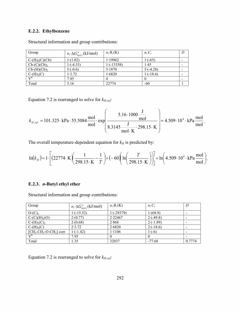
292

E.2.2. Ethylbenzene

Structural information and group contributions:

Group ni∙ ∞∆ ihydG , (kJ/mol) ni∙Bi (K) ni∙Ci D

C-(H)2(C)(Cb) 1∙(1.02) 1∙19962 1∙(-65) - Cb-(C)(Cb)2 1∙(-4.53) 1∙(-13358) 1∙45 - Cb-(H)(Cb)2 5∙(-0.6) 5∙1870 5∙(-4.28) - C-(H)3(C) 1∙3.72 1∙6820 1∙(-18.6) - Y0 7.95 0 0 - Total 5.16 22774 -60 1

Equation 7.2 is rearranged to solve for kH,ref:

molmolkPa10509.4

K15.298Kmol

J3145.8

molJ100016.5

expmolmol5084.55kPa325.101 4

, ⋅⋅=

⋅⋅⋅

⋅⋅⋅⋅=refHk .

The overall temperature-dependent equation for kH is predicted by:

( ) ( ) ( )

⋅⋅+

⋅−+

−

⋅⋅⋅=

molmolkPa10509.4ln

K15.298ln601

K15.2981K227741ln 4T

TkH .

E.2.3. n-Butyl ethyl ether

Structural information and group contributions:

Group ni∙ ∞∆ ihydG , (kJ/mol) ni∙Bi (K) ni∙Ci D

O-(C)2 1∙(-15.52) 1∙(-29379) 1∙(68.9) - C-(C)(H)2(O) 2∙(0.77) 2∙22467 2∙(-49.8) - C-(H)2(C)2 2∙(0.68) 2∙868 2∙(-1.89) - C-(H)3(C) 2∙3.72 2∙6820 2∙(-18.6) - [CH3-CH2-O-CH2] corr 1∙(-1.42) 1∙1106 1∙(-6) - Y0 7.95 0 0 - Total 1.35 32037 -77.68 0.7774

Equation 7.2 is rearranged to solve for kH,ref:

293

molmolkPa10696.9

K15.298Kmol

J3145.8

molJ100035.1

expmolmol5084.55kPa325.101 3

, ⋅⋅=

⋅⋅⋅

⋅⋅⋅⋅=refHk .

The overall temperature-dependent equation for kH is predicted by:

( ) ( ) ( )

⋅⋅+

⋅−+

−

⋅⋅⋅=

molmolkPa10696.9ln

K15.298ln68.771

K15.2981K320377774.0ln 3T

TkH