APSC 174 Lecture Notes - Queen's Universitymath237/APSC174LectureNotes.pdfAPSC 174 Lecture Notes c...
176
APSC 174 Lecture Notes c Abdol-Reza Mansouri Queen’s University Winter 2009
Transcript of APSC 174 Lecture Notes - Queen's Universitymath237/APSC174LectureNotes.pdfAPSC 174 Lecture Notes c...
APSC 174
Lecture Notes
c©Abdol-Reza Mansouri
Queen’s UniversityWinter 2009


3
About These Notes
Dear APSC-174 student,
These notes are meant to be detailed and expanded versions of the classroomlectures you will be attending. The logical sections in these lecture notes havebeen regrouped under the term “lecture”, and these may not necessarily havean exact correspondence with the individual classroom lectures; indeed, somelectures in these lecture notes may necessitate two or three classroom lectureinstallments.
These lecture notes are still very much work in progress, and will be com-pleted as the classroom lectures progress. Some of the lecture notes may evenbe updated and slightly modified after the corresponding classroom lectureshave been delivered. It is therefore recommended that you always refer tothe latest version of these lecture notes, which will be posted on the coursewebsite.
It is strongly recommended that you read these lecture notes carefully as acomplement to the classroom lectures. Almost every lecture in these notescontains examples which have been worked out in detail. It is strongly rec-ommended that you examine those in detail, and it is equally strongly rec-ommended that you work out in detail the examples that have been left tothe reader.
Since these notes are meant for you, I would appreciate any feedback youcould give me about them. I hope you will find these notes useful, and I lookforward to hearing from you.
Abdol-Reza Mansouri

4

Contents
Lecture 1 1
Lecture 2 9
Lecture 3 21
Lecture 4 27
Lecture 5 37
Lecture 6 47
Lecture 7 59
Lecture 8 73
Lecture 9 85
Lecture 10 101
Lecture 11 121
Lecture 12 127
Lecture 13 139
Lecture 14 157
5

Lecture 1
Study Topics
• Systems of Linear Equations
• Number of Solutions to Systems of Linear Equations
1
2 LECTURE 1
Linear algebra is ubiquitous in engineering, mathematics, physics, and eco-nomics. Indeed, many problems in those fields can be expressed as problemsin linear algebra and solved accordingly. An important example of applica-tion of linear algebra which we will use as an illustration throughout theselectures, and as a motivation for the theory, is the problem of solving a sys-tem of linear equations. Systems of linear equations appear in all problemsof engineering; for example, the problem of computing currents or node volt-ages in a passive electric circuit, as well as computing forces and torques ina mechanical system lead to systems of linear equations.By a system of linear equations (with real coefficients), we mean a set ofequations of the form:
(E)
a11x1 + a12x2 + a13x3 + · · ·a1nxn = b1
a21x1 + a22x2 + a23x3 + · · ·a2nxn = b2
a31x1 + a32x2 + a33x3 + · · ·a3nxn = b3
am1x1 + am2x2 + am3x3 + · · ·amnxn = bm
where the real numbers a11, a12, · · · , a1n, a21, a22, · · · , a2n, · · · , am1, am2, · · · , amn
and b1, b2, · · · , bm are given real numbers, and we wish to solve for the realnumbers x1, x2, · · · , xn; equivalently, we wish to solve for the n−tuple of realnumbers (x1, x2, · · · , xn). Each n−tuple (x1, x2, · · · , xn) of real numbers sat-isfying the system (E) is called a solution of the system of linear equations(E). In this system, the integer m is called the number of equations,whereas the integer n is called the number of unknowns. Here are a fewexamples of systems of linear equations:
(a) Consider the system{
2x = 3,
where we wish to solve for the real number x; this is a system of linearequations with one equation (i.e. m = 1) and one unknown (i.e. n = 1).
(b) Consider now the system{
2x = 3,3x = 4,
where again we wish to solve for the real number x; this is a systemof linear equations with two equations (i.e. m = 2) and one unknown(i.e. n = 1).

3
(c) Consider now the system
{2x + y = 2,x − y = 3,
where we now wish to solve for the real numbers x and y, or, equiv-alently, for the pair of real numbers (x, y); this is a system of linearequations with two equations (i.e. m = 2) and two unknowns (i.e.n = 2).
(d) Consider now the system
{x + y + z = 0,
y − z = 3,
where we now wish to solve for the real numbers x, y and z, or, equiva-lently, for the triple of real numbers (x, y, z); this is a system of linearequations with two equations (i.e. m = 2) and three unknowns (i.e.n = 3).
Now that it is clear what we mean by a system of m linear equations in nunknowns, let us examine some examples. Let us begin with the simplestpossible example, that is, a system of linear equations with one equation(m = 1) and one unknown (n = 1).To start things off, consider the following system:
(A){
2x = 3,
where we wish to solve for the unknown real number x. Multiplying bothsides of the equation 2x = 3 by 1
2, we obtain the equation:
1
22x =
1
23,
which, upon simplification, yields:
x =3
2.
We conclude that the system of linear equations (A) has a unique solution,and it is given by the real number x = 3
2.

4 LECTURE 1
Let us still deal with the simplest case of systems of linear equations with oneequation and one unknown (i.e. m = n = 1), and consider now the system:
(B){
0x = 0,
where we again wish to solve for the real number x. It is clear that anyreal number x satisfies the equation 0x = 0; we conclude therefore that thesystem (B) has infinitely many solutions.Still remaining with the simplest case of systems of linear equations withone equation and one unknown (i.e. m = n = 1), consider now instead thesystem:
(C){
0x = 2,
where we again wish to solve for the real number x. It is clear that there isno real number x that satisfies the equation 0x = 2; we conclude thereforethat the system (C) has no solution.We can recapitulate our findings for the three examples that we consideredas follows:
• System (A) has exactly one solution.
• System (B) has infinitely many solutions.
• System (C) has no solution.
Let us now increase the complexity by one notch and examine systems oflinear equations with 2 equations and 2 unknowns (i.e. m = n = 2). Tobegin with, let us consider the following system:
(A′)
{x + y = 2,x − y = 1,
where we wish to solve for the pair (x, y) of real numbers. If the pair (x, y)is a solution of the system (A′), then we obtain from the first equation thatx = 2 − y and from the second equation that x = 1 + y. Hence, if the pair(x, y) is a solution of the system (A′), then we must have x = 2 − y andx = 1 + y; this in turn implies that we must have 2 − y = 1 + y, which thenimplies that 2y = 1, from which we obtain that y = 1
2. From the relation

5
x = 2− y, we then obtain that x = 2− 12
= 32. Note that we could have also
used the relation x = 1 + y instead, and we would still have obtained x = 32.
What we have therefore established is that if the pair (x, y) is a solution ofthe system (A′), then we must have x = 3
2and y = 1
2, i.e., the pair (x, y)
must be equal to the pair (32, 1
2); conversely, it is easy to verify, by simply
substituting in values, that the pair (32, 1
2) is actually a solution to the system
(A′); indeed, we have:
3
2+
1
2=
4
2= 2,
3
2− 1
2=
2
2= 1,
as expected. We conclude therefore that the system (A′) of linear equationshas exactly one solution, and that this solution is given by the pair (3
2, 1
2).
Consider now the following system of linear equations, again having 2 equa-tions (i.e. m = 2) and 2 unknowns (i.e. n = 2):
(B′)
{x + y = 1,
2x + 2y = 2,
where again we wish to solve for the pair (x, y) of real numbers. Applyingthe same “method” as previously, we obtain the relation x = 1 − y fromthe first equation and the relation 2x = 2 − 2y from the second equation;multiplying both sides of this last relation by 1
2yields, upon simplification
x = 1 − y. Proceeding as before, we use the two relations obtained, namelyx = 1 − y and x = 1 − y, obtaining as a result the equation 1 − y = 1 − y,which then yields 0y = 0. Clearly, any real number y satisfies the relation0y = 0, and for each such y, the corresponding x is given by x = 1 − y. Inother words, if the pair (x, y) is a solution of the system (B′), then we musthave x = 1 − y, i.e., we must have (x, y) = (1 − y, y). Conversely, for anyreal number y, the pair (1 − y, y) is a solution of the system (B′), as can bedirectly verified. Indeed,
(1 − y) + y = 1,
2(1 − y) + 2y = 2 − 2y + 2y = 2,
as expected. We conclude from these manipulations that the system (B′) oflinear equations has infinitely many solutions, and they are all of the form(1 − y, y) with y any real number.

6 LECTURE 1
Consider now the following system of linear equations, again having 2 equa-tions (i.e. m = 2) and 2 unknowns (i.e. n = 2):
(C ′)
{x + y = 1,
2x + 2y = 0,
where again we wish to solve for the pair (x, y) of real numbers. Applyingthe same “method” as previously, we obtain the relation x = 1 − y fromthe first equation, and the relation 2x = −2y from the second equation;multiplying both sides of this last relation by 1
2yields, upon simplification,
the relation x = −y. We have therefore that if the pair (x, y) is a solutionof system (C ′), then we must have x = 1 − y and x = −y, and hence, wemust also have as a result that 1− y = −y, which yields 0y = 1. Since thereexists no real number y such that 0y = 1, we conclude that there exists nopair (x, y) of real numbers which would be a solution to system (C ′). Weconclude therefore that system (C ′) has no solution.We recapitulate our findings concerning systems (A′), (B′) and (C ′) as fol-lows:
• System (A′) has exactly one solution.
• System (B′) has infinitely many solutions.
• System (C ′) has no solution.
Note that these are exactly the cases that we encountered for the systems(A), (B) and (C), which consisted of only one equation in one unknown. Avery natural question that comes to mind at this point is: Can a system oflinear equations, with whatever number of equations and whatever numberof unknowns, have a number of solutions different from these, i.e. a numberof solutions different from 0, 1 and ∞ ? For example, can we come up witha system of linear equations that has exactly 2 solutions ? or exactly 17solutions ? or 154 solutions ? ... Is there anything special with 0, 1,∞, ordid we stumble on these by accident ? ... and many such questions.We shall see in the next few lectures that these are the only cases that wecan encounter with systems of linear equations; that is, a system of linearequations, with whatever number of equations and whatever number of un-knowns, can have either exactly one solution, infinitely many solutions,
7
or no solution at all; it is instructive to contrast this with the case of poly-nomial equations of degree 2 in one real variable, i.e. equations of theform ax2 +bx+c = 0, with a 6= 0, which we know can never have infinitelymany solutions (recall that they can have exactly 0, 1, or 2 solutions).In order to get to a point where we can prove this non-trivial result, we shallfirst develop the necessary tools. This will be done in the next few lectures.
PROBLEMS:
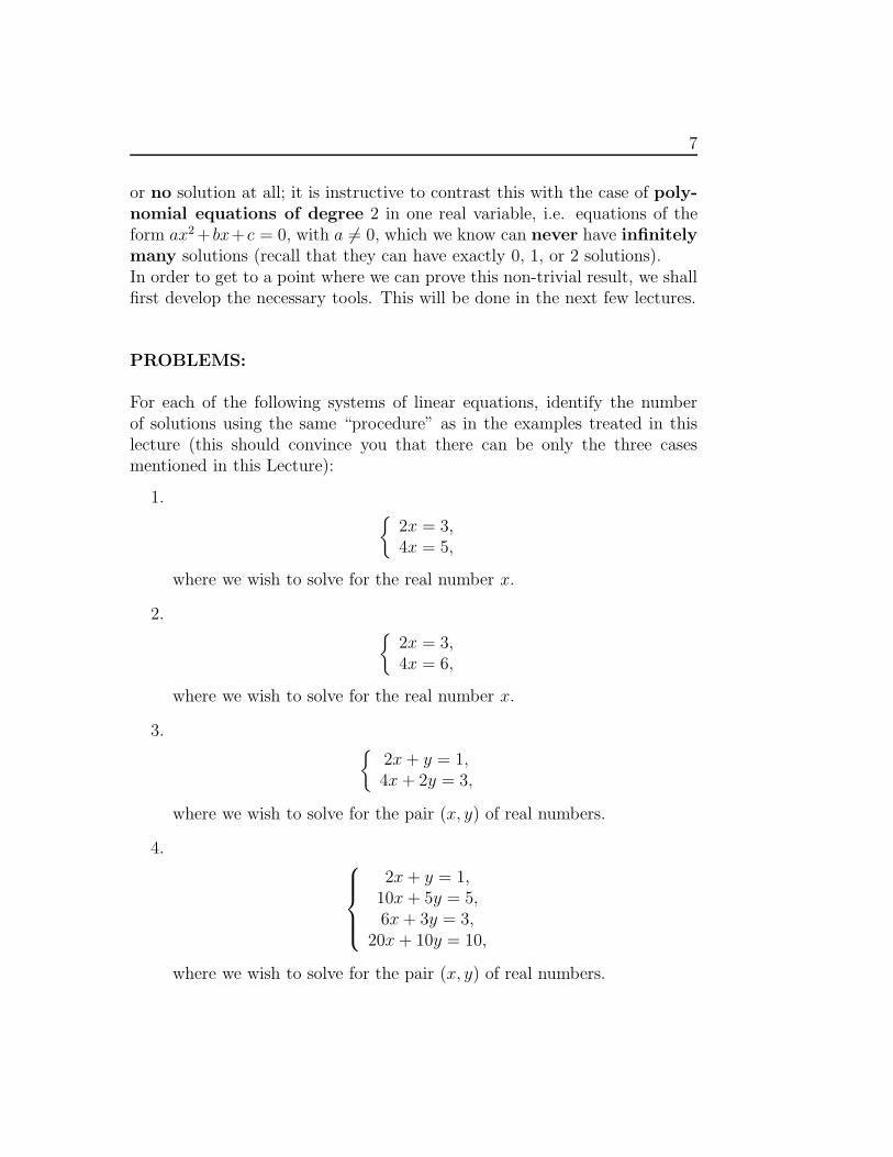
For each of the following systems of linear equations, identify the numberof solutions using the same “procedure” as in the examples treated in thislecture (this should convince you that there can be only the three casesmentioned in this Lecture):
1.{
2x = 3,4x = 5,
where we wish to solve for the real number x.
2.{
2x = 3,4x = 6,
where we wish to solve for the real number x.
3.{
2x + y = 1,4x + 2y = 3,
where we wish to solve for the pair (x, y) of real numbers.
4.
2x + y = 1,10x + 5y = 5,6x + 3y = 3,
20x + 10y = 10,
where we wish to solve for the pair (x, y) of real numbers.

8 LECTURE 1
5.
2x + y = 1,10x + 5y = 5,
x − y = 1,
where we wish to solve for the pair (x, y) of real numbers.
6.
2x − y + z = 0,x + y = 2,x − y = 1,y − z = 0,
where we wish to solve for the triple (x, y, z) of real numbers.
7.{
x + y − z = 0,
where we wish to solve for the triple (x, y, z) of real numbers.
8.
x + y − z = 0,x + y = 1,y + z = 2,
where we wish to solve for the triple (x, y, z) of real numbers.
9.{
x + y − z − w = 0,x + y = 2,
where we wish to solve for the quadruple (x, y, z, w) of real numbers.
10.
x + y − z − w = 0,−x − y = 2,z + w = 3,
where we wish to solve for the quadruple (x, y, z, w) of real numbers.

Lecture 2
Study Topics
• Real vector spaces
• Examples of real vector spaces
9
10 LECTURE 2
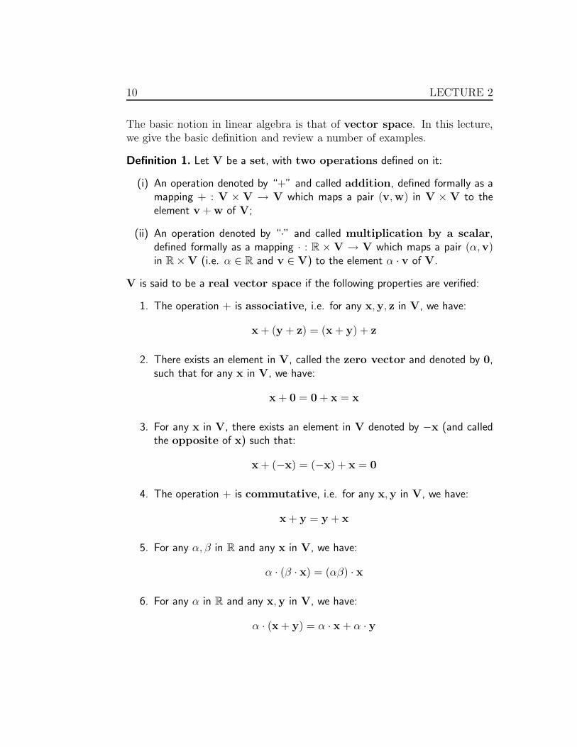
The basic notion in linear algebra is that of vector space. In this lecture,we give the basic definition and review a number of examples.
Definition 1. Let V be a set, with two operations defined on it:
(i) An operation denoted by “+” and called addition, defined formally as amapping + : V × V → V which maps a pair (v,w) in V × V to theelement v + w of V;
(ii) An operation denoted by “·” and called multiplication by a scalar,defined formally as a mapping · : R × V → V which maps a pair (α,v)in R × V (i.e. α ∈ R and v ∈ V) to the element α · v of V.
V is said to be a real vector space if the following properties are verified:
1. The operation + is associative, i.e. for any x,y, z in V, we have:
x + (y + z) = (x + y) + z
2. There exists an element in V, called the zero vector and denoted by 0,such that for any x in V, we have:
x + 0 = 0 + x = x
3. For any x in V, there exists an element in V denoted by −x (and calledthe opposite of x) such that:
x + (−x) = (−x) + x = 0
4. The operation + is commutative, i.e. for any x,y in V, we have:
x + y = y + x
5. For any α, β in R and any x in V, we have:
α · (β · x) = (αβ) · x
6. For any α in R and any x,y in V, we have:
α · (x + y) = α · x + α · y

11
7. For any α, β in R and any x in V, we have:
(α + β) · x = α · x + β · x
8. For any x in V, we have:
1 · x = x
We shall usually denote the vector space by (V, +, ·) and sometimes only byV, when there is no risk of confusion about what the addition and multipli-cation by scalar operation are. Each element of V is called a vector.We now examine a number of examples in order to develop some familiaritywith this concept.
(a) Consider the usual set R of real numbers, with the addition operation“+” being the usual addition of real numbers, and the multiplication byscalar operation “·” the usual multiplication operation of real numbers.It is easy to verify that, with these two operations, R satisfies all theaxioms of a real vector space. We can write therefore that (R, +, ·) isa real vector space.
(b) Let R2 denote the set of all pairs (x, y) with x and y real numbers.
We define an addition operation “+” on R2 as follows: If (x1, y1) and
(x2, y2) are two elements of R2, we define:
(x1, y1) + (x2, y2) = (x1 + x2, y1 + y2).
We also define a multiplication by scalar operation “·” on R2 as follows:
For any α in R and any (x, y) in R2, we define:
α · (x, y) = (αx, αy).
It is easy to verify that endowed with these two operations, R2 satisfies
all the axioms of a real vector space. We can write therefore that(R2, +, ·) is a real vector space.
(c) Let F(R; R) denote the set of all functions f : R → R, i.e. the set ofall real-valued functions of a real variable. We define the addition op-eration “+” on F(R; R) as follows: If f, g are two elements of F(R; R),we define (f + g) : R → R by:
(f + g)(t) = f(t) + g(t), for all t in R.
12 LECTURE 2
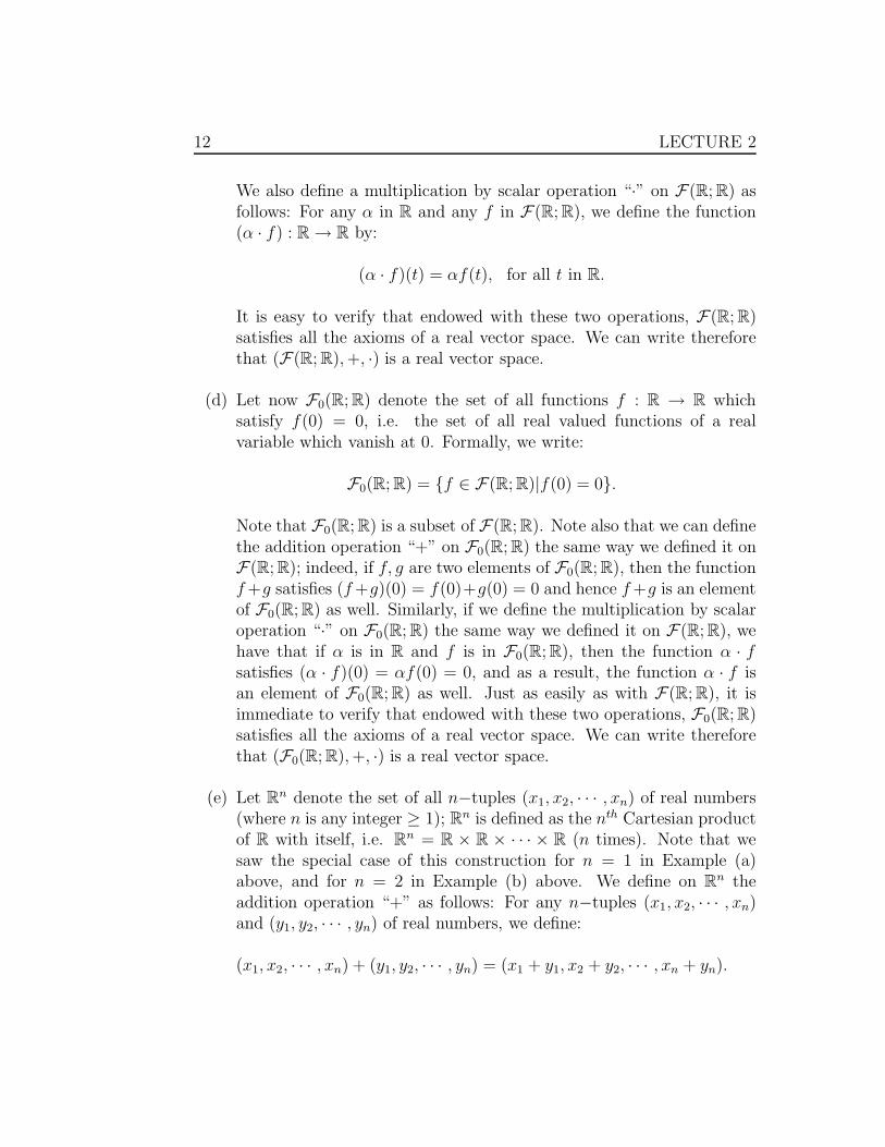
We also define a multiplication by scalar operation “·” on F(R; R) asfollows: For any α in R and any f in F(R; R), we define the function(α · f) : R → R by:
(α · f)(t) = αf(t), for all t in R.
It is easy to verify that endowed with these two operations, F(R; R)satisfies all the axioms of a real vector space. We can write thereforethat (F(R; R), +, ·) is a real vector space.
(d) Let now F0(R; R) denote the set of all functions f : R → R whichsatisfy f(0) = 0, i.e. the set of all real valued functions of a realvariable which vanish at 0. Formally, we write:
F0(R; R) = {f ∈ F(R; R)|f(0) = 0}.
Note that F0(R; R) is a subset of F(R; R). Note also that we can definethe addition operation “+” on F0(R; R) the same way we defined it onF(R; R); indeed, if f, g are two elements of F0(R; R), then the functionf +g satisfies (f +g)(0) = f(0)+g(0) = 0 and hence f +g is an elementof F0(R; R) as well. Similarly, if we define the multiplication by scalaroperation “·” on F0(R; R) the same way we defined it on F(R; R), wehave that if α is in R and f is in F0(R; R), then the function α · fsatisfies (α · f)(0) = αf(0) = 0, and as a result, the function α · f isan element of F0(R; R) as well. Just as easily as with F(R; R), it isimmediate to verify that endowed with these two operations, F0(R; R)satisfies all the axioms of a real vector space. We can write thereforethat (F0(R; R), +, ·) is a real vector space.
(e) Let Rn denote the set of all n−tuples (x1, x2, · · · , xn) of real numbers
(where n is any integer ≥ 1); Rn is defined as the nth Cartesian product
of R with itself, i.e. Rn = R × R × · · · × R (n times). Note that we
saw the special case of this construction for n = 1 in Example (a)above, and for n = 2 in Example (b) above. We define on R
n theaddition operation “+” as follows: For any n−tuples (x1, x2, · · · , xn)and (y1, y2, · · · , yn) of real numbers, we define:
(x1, x2, · · · , xn) + (y1, y2, · · · , yn) = (x1 + y1, x2 + y2, · · · , xn + yn).

13
We also define a multiplication by scalar operation “·” on Rn as follows:
For any α in R and any element (x1, x2, · · · , xn) of Rn, we define:
α · (x1, x2, · · · , xn) = (αx1, αx2, · · · , αxn).
It is easy to verify that endowed with these two operations, Rn satisfies
all the axioms of a real vector space. We can write therefore that(Rn, +, ·) is a real vector space.
(f) Let (Rn)0 denote the set of all n−tuples (x1, x2, · · · , xn) of real numberswhich satisfy x1 +x2 + · · ·+ xn = 0. Note that (Rn)0 is a subset of R
n.Furthermore, we can define on (Rn)0 the addition operation “+” andthe multiplication by scalar operation “·” in exactly the same way thatwe defined them on R
n. Indeed, if (x1, x2, · · · , xn) and (y1, y2, · · · , yn)are two elements of (Rn)0, then the n−tuple (x1+y1, x2+y2, · · · , xn+yn)is also in (Rn)0 since
(x1 + y1) + · · ·+ (xn + yn) = (x1 + · · ·+ xn) + (y1 + · · ·+ yn)
= 0 + 0
= 0.
Similarly, if α is in R and (x1, x2, · · · , xn) is an element of (Rn)0, thenthe n−tuple α · (x1, x2, · · · , xn) is also in (Rn)0, since
αx1 + αx2 + · · ·αxn = α(x1 + x2 + · · ·+ xn)
= 0.
It is easy to verify that endowed with these two operations, (Rn)0 sat-isfies all the axioms of a real vector space. We can write therefore that((Rn)0, +, ·) is a real vector space.
Let us now consider examples of sets with operations on them which do notmake them real vector spaces:
(g) On the set Rn, which we have defined in Example (e) above, define an
addition operation, which we denote by + to distinguish it from the onedefined in Example (e), as follows: For any n−tuples (x1, x2, · · · , xn)and (y1, y2, · · · , yn) of real numbers, define:
(x1, x2, · · · , xn)+(y1, y2, · · · , yn) = (x1 + 2y1, x2 + 2y2, · · · , xn + 2yn).

14 LECTURE 2
Define the multiplication by scalar operation “·” as in Example (e). Itis easy to verify that endowed with these two operations, R
n does notsatisfy all the axioms of a real vector space. We can therefore writethat (Rn, +, ·) is not a real vector space.
(h) On the set F(R; R), defined in Example (c) above, define the additionoperation + exactly as in Example (c), but define the multiplication byscalar operation by · (to distinguish it from the one defined in Example(c)) as follows: For any α in R and f in F(R; R), define the elementα·f of F(R; R) as follows:
(α·f)(t) = α(f(t))2, for all t in R.
It is easy to verify that endowed with these two operations F(R; R)does not satisfy all the axioms of a real vector space. We can writetherefore that (F(R; R), +, ·) is not a real vector space.
Now that the concept of real vector space is hopefully getting more concrete,let us prove the following simple (and very intuitive) results for general vectorspaces:
Theorem 1. Let (V, +, ·) be a real vector space. Then:
• For any v in V, we have 0 · v = 0;
• For any α in R, we have α · 0 = 0.
Proof. Let us first prove the first statement. Since 0 = 0 + 0, we have, ofcourse:
0 · v = (0 + 0) · v = 0 · v + 0 · v,
where we have used Property (7) of a vector space to get this last equality;now by property (3) of a vector space, there exists an element in V, whichwe denote by −0 ·v, such that −0 ·v + 0 ·v = 0; adding −0 ·v to both sidesof the above equality yields:
−0 · v + 0 · v = −0 · v + (0 · v + 0 · v),
which, by Property (1) of a vector space is equivalent to the equality:
−0 · v + 0 · v = (−0 · v + 0 · v) + 0 · v,

15
which, by the fact that −0 · v + 0 · v = 0 (Property (3)) is equivalent to theequality
0 = 0 + 0 · v,
which, by Property (2) of a vector space, is equivalent to
0 = 0 · v,
i.e. 0 · v = 0.Let us now prove the second statement. Since 0 = 0 + 0 (Property (2)), wehave:
α · 0 = α · (0 + 0) = α · 0 + α · 0,
where we have used Property (6) to get this last equality; By property (3),there exists an element in V, which we denote by −α · 0, such that −α · 0 +α · 0 = 0; adding −α · 0 to both sides of the above equality yields:
−α · 0 + α · 0 = −α · 0 + (α · 0 + α · 0),
which, by Property (1) is equivalent to
−α · 0 + α · 0 = (−α · 0 + α · 0) + α · 0,
which by the fact that −α · 0 + α · 0 = 0 (Property (3)) is equivalent to theequality
0 = 0 + α · 0,
which, by Property (2), is equivalent to
0 = α · 0,
i.e., α · 0 = 0.
Before closing this section, we consider an important example of a real vectorspace which we will deal with very frequently. We denote it by Rn (to dis-tinguish it from R
n) and call it the vector space of all column n−vectorswith real entries. It is the set of all elements of the form
x1
x2...
xn
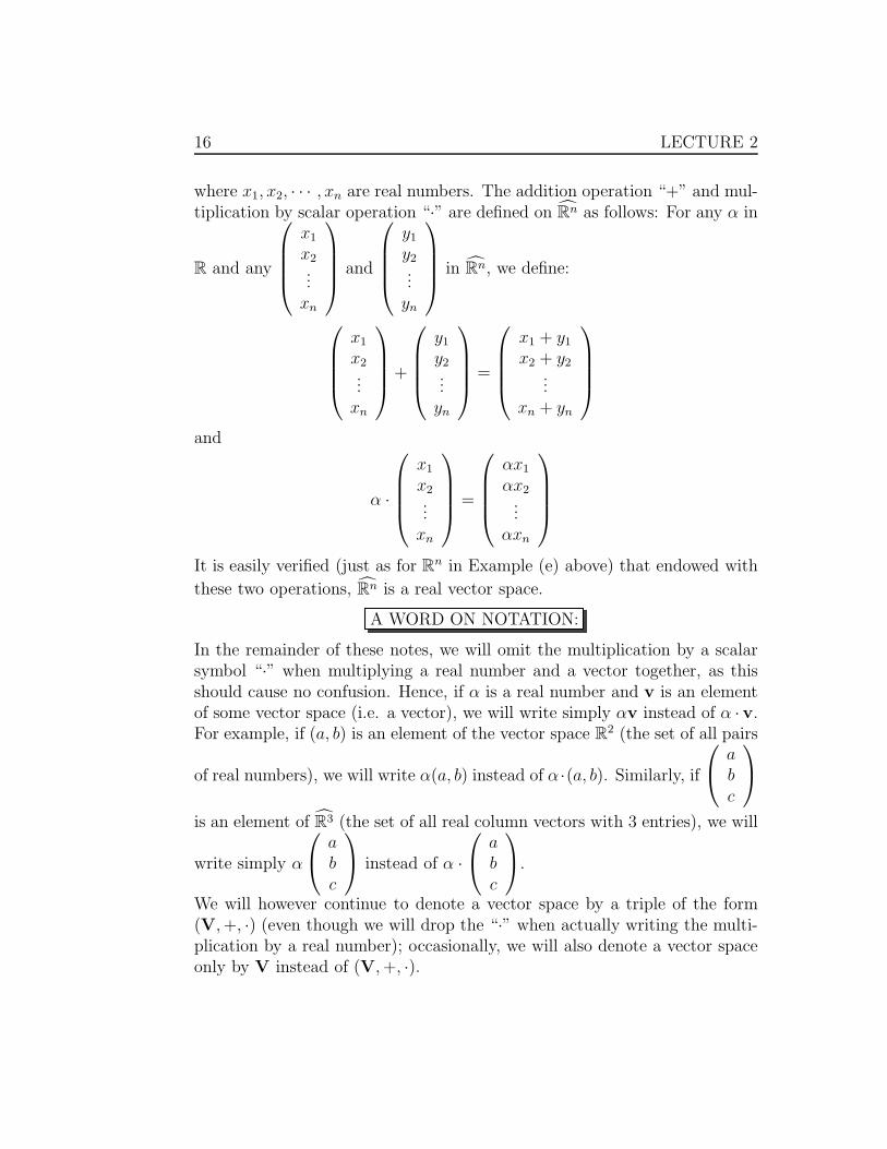
16 LECTURE 2
where x1, x2, · · · , xn are real numbers. The addition operation “+” and mul-tiplication by scalar operation “·” are defined on Rn as follows: For any α in
R and any
x1
x2...
xn
and
y1
y2...
yn
in Rn, we define:
x1
x2...
xn
+
y1
y2...yn
=
x1 + y1
x2 + y2...
xn + yn
and
α ·
x1
x2...
xn
=
αx1
αx2...
αxn
It is easily verified (just as for Rn in Example (e) above) that endowed with
these two operations, Rn is a real vector space.
A WORD ON NOTATION:
In the remainder of these notes, we will omit the multiplication by a scalarsymbol “·” when multiplying a real number and a vector together, as thisshould cause no confusion. Hence, if α is a real number and v is an elementof some vector space (i.e. a vector), we will write simply αv instead of α · v.For example, if (a, b) is an element of the vector space R
2 (the set of all pairs
of real numbers), we will write α(a, b) instead of α ·(a, b). Similarly, if
abc
is an element of R3 (the set of all real column vectors with 3 entries), we will
write simply α
abc
instead of α ·
abc
.
We will however continue to denote a vector space by a triple of the form(V, +, ·) (even though we will drop the “·” when actually writing the multi-plication by a real number); occasionally, we will also denote a vector spaceonly by V instead of (V, +, ·).
17
PROBLEMS:
1. Show that the set of all nonnegative integers N = {0, 1, 2, 3, · · · }, withaddition and multiplication defined as usual is not a real vector space,and explain precisely why.
2. Show that the set of all integers Z = {· · · ,−3,−2,−1, 0, 1, 2, 3, · · · },with addition and multiplication defined as usual is not a real vectorspace, and explain precisely why.
3. Show that the set of all non-negative real numbers R+ = {x ∈ R|x ≥ 0}
(with addition and multiplication defined as for R) is not a real vectorspace, and explain precisely why.
4. Show that the set of all non-positive real numbers R− = {x ∈ R|x ≤ 0}
(with addition and multiplication defined as for R) is not a real vectorspace, and explain precisely why.
5. Show that the subset of R defined by S = {x ∈ R| − 1 ≤ x ≤ 1} (withaddition and multiplication defined as for R) is not a real vector space,and explain precisely why.
6. Let F1(R; R) be the set of all functions f : R → R which satisfyf(0) = 1. Show that with addition and multiplication defined as forF(R; R) (see Example (c) of this Lecture), F1(R; R) is not a real vectorspace, and explain precisely why.
7. Let F[−1,1](R; R) be the set of all functions f : R → R which satisfy−1 ≤ f(x) ≤ 1, for all x ∈ R. Show that with addition and mul-tiplication defined as for F(R; R) (see Example (c) of this Lecture),F[−1,1](R; R) is not a real vector space, and explain precisely why.
8. Consider the set R2 of all pairs (x, y) of real numbers. Define an “ad-
dition” operation, which we denote by “+”, as follows: For any (x, y)and (u, v) in R
2, we define (x, y)+(u, v) to be the pair (y + v, x + u).Define the multiplication operation · as in Example (b) (i.e. α ·(x, y) =(αx, αy)). Is (R2, +, ·) a real vector space ? Explain precisely why orwhy not.
9. Consider the set R2 of all pairs (x, y) of real numbers. Define an “ad-
dition” operation, which we again denote by “+”, as follows: For

18 LECTURE 2
any (x, y) and (u, v) in R2, we define (x, y)+(u, v) to be the pair
(x + v, y + u). Define the multiplication operation · as in Example(b) (i.e. α · (x, y) = (αx, αy)). Is (R2, +, ·) a real vector space ? Ex-plain precisely why or why not.
10. Consider the subset V1 of R2 consisting of all pairs (x, y) of real numbers
such that x + y = 1. If we define the addition and multiplicationoperations on V1 as we did for R
2 in Example (b) of this Lecture, dowe obtain a real vector space ? Explain precisely why or why not.
11. Consider the subset V2 of R2 consisting of all pairs (x, y) of real numbers
such that x + y = 0. If we define the addition and multiplicationoperations on V2 as we did for R
2 in Example (b) of this Lecture, dowe obtain a real vector space ? Explain precisely why or why not.
12. Consider now the subset V3 of R2 consisting of all pairs (x, y) of real
numbers such that 2x− 3y = 1. If we define the addition and multipli-cation operations on V3 as we did for R
2 in Example (b) of this Lecture,do we obtain a real vector space ? Explain precisely why or why not.
13. Consider now the subset V3 of R2 consisting of all pairs (x, y) of real
numbers such that 2x− 3y = 0. If we define the addition and multipli-cation operations on V4 as we did for R
2 in Example (b) of this Lecture,do we obtain a real vector space ? Explain precisely why or why not.
14. Let a1, a2, · · · , an be given real numbers, and consider the subset V ofR
n (defined in Example (e) of this Lecture) consisting of all n−tuples(x1, x2, · · · , xn) of real numbers which satisfy
a1x1 + a2x2 + · · · + anxn = 0.
With addition and multiplication operations defined as in Example (e)of this Lecture, is V a real vector space ? Explain precisely why orwhy not.
15. Let a1, a2, · · · , an be given real numbers, and consider the subset V ofR
n (defined in Example (e) of this Lecture) consisting of all n−tuples(x1, x2, · · · , xn) of real numbers which satisfy
a1x1 + a2x2 + · · · + anxn = 1.
19
With addition and multiplication operations defined as in Example (e)of this Lecture, is V a real vector space ? Explain precisely why orwhy not.
16. Let a1, a2, · · · , an be given real numbers, and consider the subset W ofR
n (defined in Example (e) of this Lecture) consisting of all n−tuples(x1, x2, · · · , xn) of real numbers which satisfy
a1x1 + a2x2 + · · ·+ anxn ≥ 0.
With addition and multiplication operations defined as in Example (e)of this Lecture, is W a real vector space ? Explain precisely why orwhy not.
17. Let S = {ξ} be a set consisting of a single element, denoted ξ. Definethe addition operation “+” on S as follows: ξ + ξ = ξ, and definethe multiplication (by a scalar) operation “·” on S as follows: For anyα ∈ R, α · ξ = ξ. Show that (S, +, ·) is a real vector space.
18. Let (V, +, ·) be a real vector space. By the definition of a real vectorspace (see Property (2)), we know that there exists a “special” elementin V, which we denote by 0 and call the zero vector of V, which hasthe property that for any v in V, v +0 = 0+v = v. We wish to showthat this “special” element is actually unique. To do so, prove that ifsome (possibly other) element of V, call it 0, satisfies Property (2) ofa real vector space, then we must have 0 = 0, i.e. there is no elementin V other than the zero vector 0 itself, which satisfies Property (2).

20 LECTURE 2

Lecture 3
Study Topics
• Vector subspaces
• Examples and properties of vector subspaces
21

22 LECTURE 3
We now define another important notion, that of a subspace of a vectorspace.
Definition 2. Let (V, +, ·) be a real vector space, and let W be a subset of V(i.e. W ⊂ V). W is said to be a vector subspace (or, for short, subspace)of (V, +, ·) (or, for short, of V) if the following properties hold:
(i) The zero element 0 of V is in W, that is, 0 ∈ W.
(ii) For any x and y in W, we have x + y ∈ W.
(iii) For any α in R and any x in W, we have αx ∈ W.
Before going further, we examine a number of examples:
(a) Recall the real vector space (Rn, +, ·) of all real n−tuples (x1, x2, · · · , xn)which was defined in Lecture 2; recall also the subset (Rn)0 of R
n (de-fined in the same lecture), consisting of all n−tuples (x1, x2, · · · , xn)in R
n for which x1 + x2 + · · · + xn = 0 (i.e. all entries add up to0). Let us show that (Rn)0 is a vector subspace of the real vectorspace (Rn, +, ·): To do this, we have to show that properties (i),(ii),and (iii) of a vector subspace are verified. Let us begin with prop-erty (i); the zero element 0 of R
n is the n−tuple (0, 0, · · · , 0) (allzero entries); since 0 + 0 + · · · + 0 = 0, it is clear that the n-tuple(0, 0, · · · , 0) is in (Rn)0, i.e. 0 ∈ (Rn)0; hence, property (i) of a vectorsubspace is verified. Let us now check Property (ii): Let (x1, x2, · · · , xn)and (y1, y2, · · · , yn) be two elements of (Rn)0; we have to show thatthe n−tuple (x1, x2, · · · , xn) + (y1, y2, · · · , yn), which is defined as then−tuple (x1 + y1, x2 + y2, · · · , xn + yn), is in (Rn)0. Now, since
(x1 + y1) + · · ·+ (xn + yn) = (x1 + · · · + xn) + (y1 + · · · + yn)
= 0 + 0
= 0,
it follows that the n−tuple (x1 + y1, x2 + y2, · · · , xn + yn) is in (Rn)0,i.e. (x1, x2, · · · , xn) + (y1, y2, · · · , yn) is in (Rn)0. Hence Property (ii)is verified. Finally, let us check Property (iii); let then α ∈ R beany real number and let (x1, x2, · · · , xn) be any element of (Rn)0; we

23
have to show that the n−tuple α(x1, x2, · · · , xn), which is defined as(αx1, αx2, · · · , αxn), is in (Rn)0. Now, since
αx1 + αx2 + · · ·αxn = α(x1 + x2 + · · ·+ xn)
= α(0)
= 0,
it follows that the n−tuple (αx1, αx2, · · · , αxn) is in (Rn)0, i.e. α(x1, x2, · · · , xn)is in (Rn)0. Hence, Property (iii) is verified as well. We conclude that(Rn)0 is a vector subspace of the real vector space (Rn, +, ·).
(b) Let (V, +, ·) be a real vector space. Then V is itself a vector subspaceof V.
(c) Let (V, +, ·) be a real vector space. Then the set {0} consisting of thezero element 0 of V alone is a vector subspace of V.
(d) Recall the real vector space (F(R; R), +, ·) of all real-valued functionsof a real variable defined in Lecture 2, as well as the subset F0(R; R)of F(R; R) defined in the same lecture (recall F0(R; R) consists of allreal-valued functions f of a real variable for which f(0) = 0). It is easyto verify that F0(R; R) is a vector subspace of F(R; R).
For completeness, let us also consider examples of subsets which are notvector subspaces:
(e) Recall again the real vector space (Rn, +, ·) of all real n−tuples (x1, x2, · · · , xn)which was defined in Lecture 2; let (Rn)1 denote the subset of R
n con-sisting of all n−tuples (x1, x2, · · · , xn) of R
n for which x1+x2+· · ·+xn =1 (i.e. the entries add up to 1). It is easy to verify that (Rn)1 is not avector subspace of (Rn, +, ·).
(f) Recall now again the real vector space (F(R; R), +, ·) defined in Lecture2, and let F1(R; R) denote the subset of (F(R; R), +, ·) consisting ofall functions f ∈ (F(R; R), +, ·) for which f(0) = 1. It is easy to verifythat F1(R; R) is not a vector subspace of (F(R; R), +, ·).
Vector subspaces of a given vector space have the following important prop-erty:
24 LECTURE 3
Theorem 2. Let (V, +, ·) be a real vector space, and let W1 ⊂ V and W2 ⊂ Vbe two vector subspaces of V; then their intersection W1∩W2 is also a vectorsubspace of V.
Proof: To prove that W1∩W2 is a vector subspace of V , we have to verifythat W1 ∩ W2 satisfies the three properties of a vector subspace.
(i) We begin by showing the first property, namely that the zero element0 of V is in W1∩W2. Since W1 is by assumption a vector subspace ofV, the zero element 0 is in W1; similarly, since W2 is by assumptiona vector subspace of V, the zero element 0 is in W2. Hence, the zeroelement 0 is in W1 and in W2, that is, 0 is in the intersectionW1 ∩ W2 of W1 and W2.
(ii) Let us now prove the second property of a vector subspace, namelythat for any x and y in W1 ∩W2, x + y is also in W1 ∩W2. For this,let us take x and y in W1 ∩ W2; we have to show that x + y is alsoin W1 ∩ W2. Since x is in W1 ∩ W2, it is in W1; similarly, since yis in W1 ∩ W2, it is also in W1. Since by assumption W1 is a vectorsubspace of V, x + y is also in W1. We now repeat this procedure forW2 instead of W1; since x is in W1 ∩W2, it is in W2; similarly, sincey is in W1 ∩W2, it is also in W2. Since by assumption W2 is a vectorsubspace of V, x+y is also in W2. Hence, we have obtained that x+yis in W1 and in W2; hence, x + y is in W1 ∩ W2.
(ii) Let us now prove the third and last property of a vector subspace,namely that for any α in R and any x in W1 ∩ W2, then αx is inW1 ∩ W2. Since x is in W1 ∩ W2, it is in W1; since by assumptionW1 is a vector subspace of V, αx is also in W1. Similarly, since xis in W1 ∩ W2, it is also in W2; since by assumption W2 is a vectorsubspace of V, αx is also in W2. We have therefore obtained that αxis in W1 and in W2; hence, αx is in W1 ∩ W2.
We conclude that W1∩W2 satisfies the three properties of a vector subspace.This proves the theorem. �
Remark 1. It is important to note that if (V, +, ·) is a real vector space andW1,W2 two vector subspaces of V, then their union W1 ∪ W2 is in generalnot a vector subspace of V.

25
PROBLEMS:
1. Consider the real vector space (R2, +, ·) defined in Example (b) of Lec-ture 2. For each of the following subsets of R
2, determine whether ornot they are a vector subspace of R
2:
(a) S = set of all (x, y) in R2 such that 6x + 8y = 0.
(b) S = set of all (x, y) in R2 such that 6x + 8y = 1.
(c) S = set of all (x, y) in R2 such that x = 0.
(d) S = set of all (x, y) in R2 such that y = 0.
(e) S = set of all (x, y) in R2 such that x = 3.
(f) S = set of all (x, y) in R2 such that y = 5.
(g) S = set of all (x, y) in R2 such that x2 + y2 = 1.
(h) S = set of all (x, y) in R2 such that xy = 0.
(i) S = set of all (x, y) in R2 such that xy = 1.
2. Consider the real vector space (F(R; R), +, ·) defined in Example (c)of Lecture 2. For each of the following subsets of F(R; R), determinewhether or not they are a vector subspace of F(R; R):
(a) S = set of all f in F(R; R) such that f(1) = 0.
(b) S = set of all f in F(R; R) such that f(1) = 0 and f(2) = 0.
(c) S = set of all f in F(R; R) such that f(1) = f(2).
(d) S = set of all f in F(R; R) such that f(1) = 1 + f(2).
(e) S = set of all f in F(R; R) such that f(1) = f(2) and f(2) = f(3).
(f) S = set of all f in F(R; R) such that f(1) = f(2) and f(4) = 0.
(g) S = set of all f in F(R; R) such that f(x) = 0 for all −1 ≤ x ≤ 1.
(h) S = set of all f in F(R; R) such that f(x) = 2 for all −1 ≤ x ≤ 1.
(i) S = set of all f in F(R; R) such that f(x) ≥ 0 for all x ∈ R.
(j) S = set of all f in F(R; R) such that f(x) > 0 for all x ∈ R.
(k) S = set of all f in F(R; R) such that f(x) = f(−x) for all x ∈ R.
(l) S = set of all f in F(R; R) such that f(x) = −f(−x) for all x ∈ R.
26 LECTURE 3
(m) S = set of all f in F(R; R) such that f(x) + f(2x) = 0 for allx ∈ R.
(n) S = set of all f in F(R; R) such that f(x) + (f(2x))2 = 0 for allx ∈ R.
(o) S = set of all f in F(R; R) such that f(x) + f(x2 + 1) = 0 for allx ∈ R.
(p) S = set of all f in F(R; R) such that f(x) + f(x2 + 1) = 1 for allx ∈ R.
(q) S = set of all f in F(R; R) such that f(x) − f(x + 1) = 0 for allx ∈ R.
(r) S = set of all f in F(R; R) such that f(x)+f(x+1)+f(x+2) = 0for all x ∈ R.
(s) S = set of all f in F(R; R) such that f(x)+f(x+1)+f(x+2) = 1for all x ∈ R.
3. For the real vector space (R2, +, ·), defined in Example (b) of Lecture2, give an example of two vector subspaces V1 and V2 such thattheir union V1 ∪ V2 is not a vector subspace of R
2 (See Remark 1 inthis Lecture).
4. Let (V, +, ·) be a real vector space, and let the subset W of V be avector subspace of V. Show that with the same addition operation “+”and multiplication (by a scalar) operation “·” as in V, W satisfies allthe properties of a real vector space, and hence, is itself (with thosetwo operations) a real vector space.
Lecture 4
Study Topics
• Linear combinations of vectors
• Linear span of a finite set of vectors
27

28 LECTURE 4
We know that in a real vector space, we can add two vectors and multiplya vector by a real number (aka scalar). A natural question that comesto mind is: if we have a real vector space V and we take, say, two vectors v1
and v2 of V, what can we get by doing all these possible operations onthese two vectors, i.e. by taking the set of all vectors of the form αv1+βv2
(with α and β being real numbers) ?We shall examine this question in this lecture, and we shall see at the end ofthis lecture how it relates to our original problem, that of understandingsystems of linear equations.
Definition 3. Let (V, +, ·) be a real vector space, and let v1, · · · ,vp be a finitenumber of elements of V (with p ≥ 1). Any element of V of the form
α1v1 + α2v2 + · · ·+ αpvp,
with α1, α2, · · · , αp real numbers, is called a linear combination of the vectorsv1,v2, · · · ,vp. We denote by S(v1,v2,··· ,vp) the set of all linear combinationsof the vectors v1,v2, · · · ,vp, that is:
S(v1,v2,··· ,vp) = {α1v1 + α2v2 + · · ·+ αpvp|α1, α2, · · · , αp ∈ R}.
It is clear that S(v1,v2,··· ,vp) is a subset of V; indeed, since v1,v2, · · · ,vp
are in V , multiplying them by real numbers and adding them up gives ussomething still in V, since V is a vector space. So we can write:
S(v1,v2,··· ,vp) ⊂ V.
But there is more! Indeed, the following result shows that S(v1,v2,··· ,vp) isnot just any old subset of V; rather, it is a vector subspace of V:
Proposition 1. Let (V, +, ·) be a real vector space, and let v1, · · · ,vp be afinite number of elements of V (where p ≥ 1). The subset S(v1,v2,··· ,vp) of Vconsisting of all linear combinations of the vectors v1, · · · ,vp is a vectorsubspace of V.
Proof. To prove this result, we have to show that S(v1,v2,··· ,vp) satisfies thethree properties that a vector subspace of V should satisfy. We verifythese properties one by one:
(i) We have to show that the zero vector 0 of V is also an element ofS(v1,v2,··· ,vp); to do this, we have to show that the zero vector 0 can

29
be written as a linear combination α1v1 + α2v2 + · · · + αpvp ofv1,v2, · · · ,vp for some choice of the scalars α1, α2, · · · , αp. It is clearthat choosing α1, α2, · · · , αp to be all zero yields the desired linear com-bination; indeed, we can write:
0 = 0v1 + 0v2 + · · ·+ 0vp,
and this shows that the zero vector 0 can indeed be expressed asa linear combination of the vectors v1,v2, · · · ,vp; hence the zerovector 0 is an element of S(v1,v2,··· ,vp), i.e. 0 ∈ S(v1,v2,··· ,vp).
(ii) Let x and y be two elements of S(v1,v2,··· ,vp); we have to show that thevector x + y is also in S(v1,v2,··· ,vp). But since by assumption x is inS(v1,v2,··· ,vp), it must be that
x = α1v1 + α2v2 + · · ·αpvp
for some real numbers α1, α2, · · · , αp, by definition of the set S(v1,v2,··· ,vp)
itself. Similarly, since by assumption y is in S(v1,v2,··· ,vp), it must bethat
y = β1v1 + β2v2 + · · ·βpvp
for some real numbers β1, β2, · · · , βp, by definition of S(v1,v2,··· ,vp). Hence,the sum x + y of x and y can be written as:
x + y = (α1v1 + · · ·αpvp) + (β1v1 + · · ·βpvp)
= (α1 + β1)v1 + · · · (αp + βp)vp,
which shows that x+y itself is a linear combination of the vectorsv1,v2, · · · ,vp; hence x + y is an element of S(v1,v2,··· ,vp), i.e. x + y ∈S(v1,v2,··· ,vp).
(iii) Let now x be an element of S(v1,v2,··· ,vp) and γ be a real number; we haveto show that the vector γx is also in S(v1,v2,··· ,vp). Since, by assumption,x is in S(v1,v2,··· ,vp), it must be that
x = α1v1 + α2v2 + · · ·αpvp
for some real numbers α1, α2, · · · , αp, by definition of the set S(v1,v2,··· ,vp)
itself. Hence, we can write:
γx = γ(α1v1 + α2v2 + · · ·αpvp)
= (γα1)v1 + · · · (γαp)vp,

30 LECTURE 4
which shows that γx itself is a linear combination of the vectorsv1,v2, · · · ,vp; hence γx is in S(v1,v2,··· ,vp), i.e. γx ∈ S(v1,v2,··· ,vp).
We conclude that S(v1,v2,··· ,vp) satisfies all three properties of a vector sub-space of V; hence S(v1,v2,··· ,vp) is a vector subspace of V.
Before going any further, we give a name to S(v1,v2,··· ,vp):
Definition 4. The vector subspace S(v1,v2,··· ,vp) of V is called the subspaceof V generated by the vectors v1,v2, · · · ,vp; it is also called the linearspan of the vectors v1,v2, · · · ,vp.
Now that S(v1,v2,··· ,vp) has an honest name (actually two!), we examine anumber of examples:
(a) Let (V, +, ·) be a real vector space, and let v1 = 0 be the zero vectorof V. The vector subspace of V generated by v1 is clearly seen to bethe zero subspace {0} of V.
(b) Consider the real vector space (R2, +, ·) defined previously, and letv1 = (1, 0) and v2 = (0, 1); it is easy to verify that the subspace of(R2, +, ·) generated by v1,v2 is V itself.
(c) Consider the real vector space (R3, +, ·) defined previously, and considerthe two elements v1 = (1,−1, 0) and v2 = (0, 1,−1) of R
3. Let us showthat the vector subspace S(v1,v2) of R
3 spanned by v1 and v2 is the setof all (a, b, c) in R
3 such that a + b + c = 0, that is, we wish to showthat
S(v1,v2) = {(a, b, c) ∈ R3|a + b + c = 0}.
To show this equality, we will show first that we have the inclusion
S(v1,v2) ⊂ {(a, b, c) ∈ R3|a + b + c = 0},
following which we will show that we have the inclusion
{(a, b, c) ∈ R3|a + b + c = 0} ⊂ S(v1,v2);
these two inclusions will, together, show the desired equality. Let usthen begin by showing the first inclusion. For this, let us take anarbitrary element x in S(v1,v2), and show that it is also in the set

31
{(a, b, c) ∈ R3|a + b + c = 0}. By definition of S(v1,v2), x can be
written as:
x = αv1 + βv2,
for some real numbers α and β. Hence, we have:
x = αv1 + βv2
= α(1,−1, 0) + β(0, 1,−1)
= (α,−α, 0) + (0, β,−β)
= (α,−α + β,−β);
clearly, since α + (−α + β) + (−β) = 0, we have that x is in the set{(a, b, c) ∈ R
3|a + b + c = 0}. This proves the first inclusion.
To prove the second inclusion, let us take an arbitrary element y inthe set {(a, b, c) ∈ R
3|a + b + c = 0}, and show that it is also in thelinear span S(v1,v2) of v1 and v2. Let then y = (α, β, γ) ∈ {(a, b, c) ∈R
3|a + b + c = 0}; since α + β + γ = 0, we deduce that β = −(α + γ),and hence, we can write y as:
y = (α,−(α + γ), γ)
= (α,−α − γ, γ)
= (α,−α, 0) + (0,−γ, γ)
= α(1,−1, 0) + (−γ)(0, 1,−1)
= αv1 + (−γ)v2,
that is, y is a linear combination of v1 and v2 (with coefficients αand −γ, respectively) and hence is in S(v1,v2). This proves the secondinclusion, and hence, together with the first inclusion, we obtain thedesired result.
We now have enough tools at our disposal to revisit our original “exper-iments” with systems of linear equations and to have some basic under-standing of what it is that happens when a system of linear equations has asolution or has no solution. In order to make things concrete, let us considertwo examples:

32 LECTURE 4
1. Let us begin with the following system of 3 linear equation in 2 un-knowns:
(A)
x1 − x2 = 1,2x1 + x2 = 0,x1 − 2x2 = 2,
where we wish to solve for the pair (x1, x2) of real numbers. Let us
now recall the real vector space (R3, +, ·) of all column vectors of
the form
abc
where a, b, c are real numbers. Consider the elements
v1,v2,w of R3 defined as follows:
v1 =
121
,v2 =
−1
1−2
,w =
102
,
Let now x1, x2 be real numbers. We have, by definition of the operations
“+” and “·” in R3:
x1 · v1 + x2 · v2 = x1 ·
121
+ x2 ·
−1
1−2
=
x1
2x1
x1
+
−x2
x2
−2x2
=
x1 − x2
2x1 + x2
x1 − 2x2
.
Hence, the pair (x1, x2) of real numbers satisfies the system (A) of linearequations above if and only if we have:
x1 · v1 + x2 · v2 = w;
It follows immediately from this that:
• If w is not in the linear span of v1 and v2, then system (A) hasno solution,
• if w is in the linear span of v1 and v2, then system (A) has atleast one solution (but we can’t yet tell how many!).
33
2. Consider now the following system of 2 linear equations in 2 unknowns:
(B)
{x1 − x2 = 1,−x1 + x2 = 1,
where we wish to solve for the pair (x1, x2) of real numbers. In orderto understand whether this system has a solution or not, consider the
following vectors in R2:
v1 =
(1
−1
),v2 =
(−1
1
),w =
(11
).
Let now (x1, x2) be a pair of real numbers; we clearly have:
x1 · v1 + x2 · v2 = x1 ·(
1−1
)+ x2 ·
(−1
1
)=
(x1 − x2
−x1 + x2
).
It follows that the pair (x1, x2) is a solution of system (B) if and onlyif we have:
x1 · v1 + x2 · v2 = w;
Hence, we again have:
• If w is not in the linear span of v1 and v2, then system (B) hasno solution,
• if w is in the linear span of v1 and v2, then system (B) has atleast one solution (again we can’t yet tell how many!).
So we now have some basic “picture” of what it means for a system of linearequations to have, or not to have, a solution: If some given vector happensto lie in some given subspace, then the system has a solution (at least one);otherwise, it has no solution.
In order to get to a point where we can explain why that number of solutionsis always 0,1, or ∞, we have to further sharpen our tools. This is what wewill do in the following sections.
34 LECTURE 4
PROBLEMS:
1. Consider the (by now familiar) real vector space R2, consisting of all
pairs (x, y) of real numbers, with the usual addition and scalar multipli-cation operations. Consider the vectors v1,v2,v3,v4,v5 in R
2 definedas follows:
v1 = (0, 0), v2 = (1, 0), v3 = (−1, 0), v4 = (0, 3), v5 = (2, 1).
(a) Is v1 in the linear span of {v2} ?
(b) Is v1 in the linear span of {v3,v4} ?
(c) Is v2 in the linear span of {v1,v4} ?
(d) Is v2 in the linear span of {v1} ?
(e) Is v2 in the linear span of {v2,v4} ?
(f) Is v3 in the linear span of {v2} ?
(g) Is v3 in the linear span of {v4} ?
(h) Is v4 in the linear span of {v1,v2,v3} ?
(i) Is v5 in the linear span of {v2} ?
(j) Is v5 in the linear span of {v1,v2,v3} ?
(k) Is v5 in the linear span of {v2,v4} ?
(l) Is v5 in the linear span of {v3,v4} ?
2. Consider the real vector space R4 (see Lecture 2) consisting of all col-
umn vectors of the form
xyzw
with x, y, z, w real, with the usual addi-
tion and scalar multiplication operations. Define the vectors v1,v2,v3,v4
in R4 as follows:
v1 =
1000
, v2 =
2100
, v3 =
1110
, v4 =
0011
,
For each of these four vectors, determine whether they are in the linearspan of the other three.

35
3. Consider the (familiar) real vector space R3 consisting of all triples of
the form (x, y, z) with x, y, z real numbers, with the usual addition andscalar multiplication operations. For each of the following list of vectorsin R
3, determine whether the first vector is in the linear span of thelast two:
(a) (1, 1, 1), (1, 2, 1), (1, 3, 1)
(b) (0, 0, 0), (1, 2, 1), (1, 3, 1)
(c) (1, 2, 1), (1, 1, 1), (1, 3, 1)
(d) (0, 1, 0), (1, 2, 1), (1, 3, 1)
(e) (1, 1, 1), (2, 5, 0), (3, 2, 0)
(f) (1, 0, 1), (0, 2, 0), (0, 3, 0)
(g) (1, 1, 1), (0, 0, 0), (2, 2, 2)
(h) (1, 1, 0), (1, 0, 1), (0, 1, 1)
(i) (3, 2, 1), (3, 2, 2), (1, 1, 1)
(j) (0, 0, 0), (3, 2, 1), (4, 3, 1)
(k) (1, 2, 1), (2, 2, 1), (1, 3, 1)
4. Consider the real vector space F(R; R) of all real-valued functions ofa real variable (defined in Lecture 2), with the usual addition andscalar multiplication operations. Consider the elements f1, f2, f3, f4 inF(R; R), defined as follows:
f1(t) =
{0, t < 0t, t ≥ 0
f2(t) =
{0, t < 03t + 1, t ≥ 0
f3(t) =
{0, t < 0t2, t ≥ 0
f4(t) =
{0, t < 03t2 + 2t + 1, t ≥ 0
For each of these four elements (i.e. vectors) in F(R; R), verify whetheror not they are in the linear span of the other three.

36 LECTURE 4

Lecture 5
Study Topics
• Linear dependence of a set of vectors
• Linear independence of a set of vectors
37

38 LECTURE 5
Consider the vector space R2 of all pairs (x, y) of real numbers, which we
have defined previously and used numerous times. Consider the followingsubsets of R
2:
S1 = {(3, 2), (12, 8)}, S2 = {(3, 2), (0, 1)}.
What are the similarities and differences between S1 and S2 ? Well, theyboth contain two vectors each; in that, they are similar; another similarityis that they both contain the vector (3, 2). What about differences ? Noticethat the second vector in S1, namely (12, 8), is a scalar multiple of (3, 2),i.e. (12, 8) can be obtained by multiplying (3, 2) by some real number (inthis case, the real number 4); indeed, we have:
4(3, 2) = (4 × 3, 4 × 2) = (12, 8).
We can also obviously claim that (3, 2) is a scalar multiple of (12, 8) (thistime with a factor of 1
4), since we can write:
1
4(12, 8) = (
1
4× 12,
1
4× 8) = (3, 2).
On the other hand, no such thing is happening with S2; indeed, (0, 1) isnot a scalar multiple of (3, 2), since mutiplying (3, 2) by a real number cannever yield (0, 1) (prove it!). Similary, multiplying (0, 1) by a real numbercan never yield (3, 2) (prove it also!).So we have identified a fundamental difference between S1 and S2: Whereasthe two elements of S1 are related, in the sense that they are scalar multiplesof one another, those of S2 are completely unrelated (in the sense thatthey are not scalar multiples of each other).Before going further, we generalize this observation into a definition:
Definition 5. Let (V, +, ·) be a real vector space, and let S = {v1,v2, · · · ,vp}be a finite subset of V.
(i) The subset S is said to be linearly independent if the only real num-bers α1, α2, · · · , αp which yield
α1v1 + α2v2 + · · ·+ αpvp = 0
are given by α1 = α2 = · · · = αp = 0.

39
(ii) The subset S is said to be linearly dependent if it is not linearlyindependent.
Another way to re-state these definitions is as follows:
(i) The subset S is linearly independent if whenever the linear combi-nation α1v1 + · · · + αpvp is equal to 0, it must be that α1, · · · , αp areall 0.
(ii) The subset S is linearly dependent if there exist real numbers α1, · · · , αp
not all 0, but for which the linear combination α1v1 + · · ·+ αpvp is nev-ertheless equal to 0.
Before going any further, let us show that the set S1 above is a linearly de-pendent subset of R
2, and that the set S2 above is a linearly independentsubset of R
2. Let us begin with S1: Let α1 = −4 and α2 = 1; we have:
α1(3, 2) + α2(12, 8) = −4(3, 2) + 1(12, 8)
= (−12,−8) + (12, 8)
= (0, 0)
= 0
(recall that the zero element 0 of R2 is the pair (0, 0)). Hence we have
found real numbers α1, α2 which are not both zero but such that the linearcombination α1(3, 2) + α2(12, 8) is the zero vector 0 = (0, 0) of R
2. Thisproves that S1 is a linearly dependent subset of R
2.Let us now show that the set S2 above is a linearly independent subsetof R
2. To do this, we have to show that if for some real numbers α1, α2 wehave
α1(3, 2) + α2(0, 1) = (0, 0),
then, necessarily, we must have α1 = 0 and α2 = 0. Note that:
α1(3, 2) + α2(0, 1) = (3α1, 2α1) + (0, α2)
= (3α1, 2α1 + α2).
Hence, if the linear combination α1(3, 2) + α2(0, 1) is to be equal to the zerovector (0, 0) of R
2, we must have (3α1, 2α1 +α2) = (0, 0), or, equivalently, wemust have 3α1 = 0 and 2α1 + α2 = 0; the relation 3α1 = 0 implies α1 = 0,
40 LECTURE 5
and substituting this value of α1 in the second relation yields α2 = 0. Hence,we have shown that if the linear combination α1(3, 2)+α2(0, 1) is to be equalto the zero vector (0, 0) for some real numbers α1 and α2, then we musthave α1 = 0 and α2 = 0. This proves that the subset S2 of R
2 is linearlyindependent.At this point, we may wonder how these notions of linear dependence andindependence tie in with our initial observations about the subsets S1 and S2
of R2, namely, that in S1 one of the elements can be written as a scalar mul-
tiple of the other element, whereas we cannot do the same thing with the twoelements of S2; how does this relate to linear dependence and independenceof the subsets ? The answer is given in the theorem below:
Theorem 3. Let (V, +, ·) be a real vector space, and let S = {v1,v2, · · · ,vp}be a finite subset of V . Then:
(i) If S is a linearly dependent subset of V, then one of the elements ofS can be written as a linear combination of the other elements ofS;
(ii) conversely, if one of the elements of S can be written as a linear combi-nation of the other elements of S, then S is a linearly dependentsubset of V.
Proof. Let us first prove (i): Since S is assumed linearly dependent, theredo exist real numbers α1, α2, · · · , αp not all 0, such that:
α1v1 + α2v2 + · · · + αpvp = 0.
Since α1, α2, · · · , αp are not all equal to 0, at least one of them must benon-zero; Assume first that α1 is non-zero, i.e. α1 6= 0. From the aboveequality, we deduce:
α1v1 = −α2v2 − α3v3 − · · · − αpvp,
and multiplying both sides of this last equality by 1α1
(which we can do sinceα1 6= 0), we obtain:
v1 = −α2
α1v2 −
α3
α1v3 − · · · − αp
α1vp,
which shows that v1 is a linear combination of v2,v3, · · · ,vp. Now if it is α2
which happens to be non-zero, and not α1, we repeat the same procedure,
41
but with α2 and v2 instead, and we obtain that v2 is a linear combination ofv1,v3,v4, · · · ,vp. If instead, it is α3 which is non-zero, then we repeat thesame procedure with α3 and v3; and so on. Since one of the α1, α2, · · · , αp
is non-zero, we will be able to write one of the v1,v2, · · · ,vp as a linearcombination of the others.
Let us now prove (ii): Assume then, that one of the v1,v2, · · · ,vp can bewritten as a linear combination of the others. Again, for simplicity, assumeit is v1 which can be written as a linear combination of the other vectors,namely v2,v3, · · · ,vp (if it is another vector instead of v1, we do the samething for that vector); hence, there exist real numbers α2, α3, · · · , αp suchthat:
v1 = α2v2 + α3v3 + · · · + αpvp.
We can write the above equality equivalently as:
−v1 + α2v2 + α3v3 + · · ·+ αpvp = 0,
and, equivalently, as:
α1v1 + α2v2 + α3v3 + · · ·+ αpvp = 0,
where α1 = −1; but this shows that the above linear combination is the zerovector 0, and yet not all of α1, α2, · · · , αp are 0 (for the good reason thatα1 = −1). This shows that the subset S = {v1,v2, · · · ,vp} of V is linearlydependent.
We now examine a number of examples.
(a) Recall the real vector space R3 consisting of all column vectors (with 3
real entries) of the form
abc
, where a, b, c are real numbers. Con-
sider the subset S of R3 given by:
S = {
100
,
010
,
001
}.

42 LECTURE 5
Let us show that S is a linearly independent subset of R3: Let thenα1, α2, α3 be three real numbers such that
α1
100
+ α2
010
+ α3
001
=
000
;
we have to show that this implies that α1 = α2 = α3 = 0. We have:
α1
100
+ α2
010
+ α3
001
=
α1
α2
α3
,
and the equality
α1
α2
α3
=
000
does imply that α1 = α2 = α3 = 0. Hence, S is a linearly independent
subset of R3.
(b) Recall the real vector space F(R; R) of all real-valued functions on R;consider the two elements f1, f2 in F(R; R), defined as follows:
f1(t) =
{1, t < 0,0, t ≥ 0,
f2(t) =
{0, t < 0,1, t ≥ 0.
We wish to show that {f1, f2} is a linearly independent subset ofF(R; R). Let then α1, α2 be two real numbers such that
α1f1 + α2f2 = 0;
(recall that the zero element 0 of F(R; R) is defined to be the constant0 function). Hence, we must have
α1f1(t) + α2f2(t) = 0,
for all t in R; in particular, this relation should hold for t = 1 andt = −1. But for t = 1, we have:
α1f1(1) + α2f2(1) = α2,

43
and for t = −1, we get:
α1f1(−1) + α2f2(−1) = α1.
Hence we must have α2 = 0 and α1 = 0, which shows that {f1, f2} is alinearly independent subset of F(R; R).
(c) Let (V, +, ·) be any real vector space, and let S = {0} be the subset ofV consisting of the zero element alone. Let us show that S is a linearlydependent subset of V: For this, consider the linear combination 1 ·0;we evidently have 1 · 0 = 0; on the other hand, the (unique) coefficientof this linear combination (namely the real number 1) is non-zero. Thisshows that {0} is a linearly dependent subset of V.
Consider now a real vector space (V, +, ·), and let S and T be two finitesubsets of V such that S ⊂ T (i.e. S is itself a subset of T ); suppose weknow that S is a linearly dependent subset of V; what can we then sayabout T ? The following lemma does answer this question.
Lemma 1. Let (V, +, ·) be a real vector space, and S, T two finite subsets ofV such that S ⊂ T . If S is linearly dependent, then T is also linearly dependent.
Proof. Assume S has p elements and T has q elements (necessarily, we haveq ≥ p since S is a subset of T ). Let us then write:
S = {v1,v2, · · · ,vp},T = {v1,v2, · · · ,vp,vp+1,vp+2, · · · ,vq}.
Since S is by assumption a linearly dependent subset of V, there do existreal numbers α1, α2, · · · , αp not all zero, such that the linear combination
α1v1 + α2v2 + · · ·+ αpvp
is equal to the zero vector 0 of V, i.e.,
α1v1 + α2v2 + · · ·+ αpvp = 0.
But then, the linear combination
α1v1 + α2v2 + · · ·+ αpvp + 0vp+1 + · · ·+ 0vq
is also equal to 0, and yet, not all of the coefficients in the above linearcombination are zero (since not all of the α1, α2, · · · , αp are zero); this provesthat T is a linearly dependent subset of V.
44 LECTURE 5
Remark 2. Let (V, +, ·) be a real vector space. We have seen in Example (c)above that the subset {0} of V consisting of the zero vector alone is linearlydependent; it follows from the previous lemma that if S is any finite subset of Vsuch that 0 ∈ S, then S is linearly dependent.
Remark 3. The previous lemma also implies the following: If a finite subset Sof a vector space V is linearly independent, then any subset of S is linearlyindependent as well.
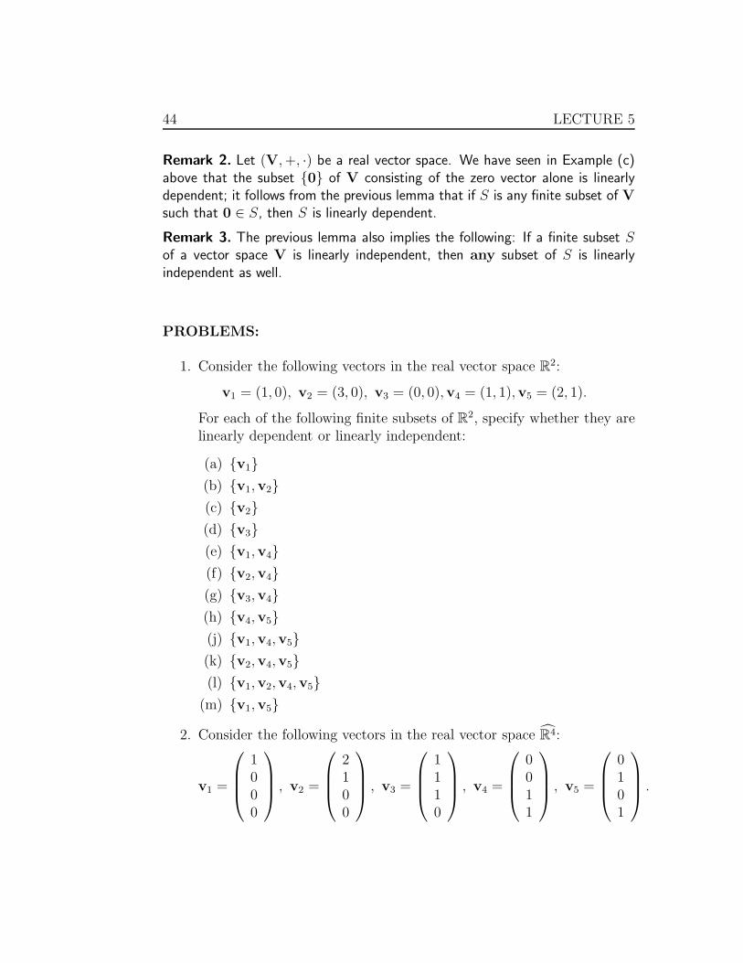
PROBLEMS:
1. Consider the following vectors in the real vector space R2:
v1 = (1, 0), v2 = (3, 0), v3 = (0, 0),v4 = (1, 1),v5 = (2, 1).
For each of the following finite subsets of R2, specify whether they are
linearly dependent or linearly independent:
(a) {v1}(b) {v1,v2}(c) {v2}(d) {v3}(e) {v1,v4}(f) {v2,v4}(g) {v3,v4}(h) {v4,v5}(j) {v1,v4,v5}(k) {v2,v4,v5}(l) {v1,v2,v4,v5}
(m) {v1,v5}
2. Consider the following vectors in the real vector space R4:
v1 =
1000
, v2 =
2100
, v3 =
1110
, v4 =
0011
, v5 =
0101
.

45
For each of the following finite subsets of R2, specify whether they are
linearly dependent or linearly independent:
(a) {v1}(b) {v1,v2}(c) {v2}(d) {v3}(e) {v1,v4}(f) {v2,v4}(g) {v3,v4}(h) {v4,v5}(j) {v1,v4,v5}(k) {v2,v4,v5}(l) {v1,v2,v4,v5}
(m) {v1,v5}(n) {v1,v2,v3,v4,v5}(o) {v3,v4,v5}(p) {v2,v3,v4,v5}
3. Consider the real vector space (F(R; R), +, ·) defined in Lecture 2, andconsider the elements f1, f2, f3, f4 in F(R; R), defined as follows:
f1(t) = 1, ∀t ∈ R,
f2(t) = t, ∀t ∈ R,
f3(t) = (t + 1)2, ∀t ∈ R,
f4(t) = t2 + 5, ∀t ∈ R,
f5(t) = t3, ∀t ∈ R,
f6(t) = t3 + 2t2, ∀t ∈ R,
For each of the following finite subsets of F(R; R), specify whether theyare linearly dependent or linearly independent:
(a) {f1}
46 LECTURE 5
(b) {f1, f2}(c) {f1, f2, f3}(d) {f1, f2, f3, f4}(e) {f2, f3, f4}(f) {f4, f5, f6}(g) {f3f4, f5, f6}(h) {f2, f3, f4, f5, f6}(j) {f1, f2, f3, f4, f5, f6}
4. Let (V, +, ·) be a real vector space, and let S be a finite subset of V.Show directly (without using Lemma 1 or Remark 2 of these lectures)that if 0 is in S then S is a linearly dependent subset of V .
Lecture 6
Study Topics
• Linear dependence/independence and linear combinations
• Application to systems of linear equations (or, we nowhave the complete answer to our initial question!)
47

48 LECTURE 6
Let (V, +, ·) be a real vector space, and let S = {v1,v2, · · · ,vp} be a finitesubset of V. We know that if the element v of V is in the linear span ofthe vectors v1,v2, · · · ,vp, then v can be written as some linear combinationof v1,v2, · · · ,vp, that is, we can find real numbers α1, α2, · · · , αp such that
α1v1 + α2v2 + · · ·αpvp = v;
A very natural question at this point is: In how many different ways canthis same v be expressed as a linear combination of v1,v2, · · · ,vp ? Doesthere exist another p−tuple of real numbers, say (γ1, γ2, · · · , γp), distinctfrom the p−tuple (α1, α2, · · · , αp) such that we also have
γ1v1 + γ2v2 + · · · γpvp = v ?
The complete answer to this question is given in the following theorems:
Theorem 4. Let (V, +, ·) be a real vector space, and let S = {v1,v2, · · · ,vp}be a finite subset of V. Let v ∈ V be in the linear span of v1,v2, · · · ,vp. IfS is a linearly independent subset of V, then v can be expressed only in aunique way as a linear combination of v1,v2, · · · ,vp; i.e., there is a uniquep−tuple (α1, α2, · · · , αp) of real numbers such that:
α1v1 + α2v2 + · · ·αpvp = v;
Proof. To prove this result, we have to show that if v (which is assumedto be in the linear span of v1,v2, · · · ,vp) can be expressed as two linearcombinations of v1,v2, · · · ,vp, then those two linear combinations must beone and the same. Assume then that we have two p−tuples of real numbers(α1, α2, · · · , αp) and (γ1, γ2, · · · , γp) such that
α1v1 + α2v2 + · · ·αpvp = v
and
γ1v1 + γ2v2 + · · · γpvp = v.
We have to show that the p−tuples (α1, α2, · · · , αp) and (γ1, γ2, · · · , γp) areequal, i.e. that α1 = γ1, α2 = γ2, · · · , αp = γp. This will show (obviously!)that those two linear combinations are exactly the same. Now these last twoequalities imply:
α1v1 + α2v2 + · · ·αpvp = γ1v1 + γ2v2 + · · · γpvp,
49
which then implies (by putting everything on the left-hand side of the “=”sign):
(α1 − γ1)v1 + (α2 − γ2)v2 + · · · (αp − γp)vp = 0;
but by linear independence of {v1,v2, · · · ,vp}, we must have:
(α1 − γ1) = (α2 − γ2) = · · · = (αp − γp) = 0,
which, equivalently, means:
α1 = γ1,
α2 = γ2,
· · ·αp = γp,
i.e. the two linear combinations
α1v1 + α2v2 + · · ·αpvp = v
and
γ1v1 + γ2v2 + · · · γpvp = v.
are one and the same.
Conversely, we have the following:
Theorem 5. Let (V, +, ·) be a real vector space, and let S = {v1,v2, · · · ,vp}be a finite subset of V. Assume that any v ∈ V be in the linear span ofv1,v2, · · · ,vp can be expressed only in a unique way as a linear combination ofv1,v2, · · · ,vp; i.e., for any v ∈ V there is a unique p−tuple (α1, α2, · · · , αp)of real numbers such that:
α1v1 + α2v2 + · · ·αpvp = v;
Then, S is a linearly independent subset of V.
50 LECTURE 6
Proof. Consider the zero vector 0 of V, and Let α1, α2, · · · , αn ∈ R be suchthat
α1v1 + α2v2 + · · · + αpvp = 0;
to show that S is linearly independent, we have to show that this last equalityimplies that α1, α2, · · · , αp are all zero. Note first that 0 is in the linear spanof v1,v2, · · · ,vp; indeed, we can write:
0 = 0v1 + 0v2 + · · · + 0vp.
Since we have assumed that any element in the linear span of v1,v2, · · · ,vp
can be written only in a unique way as a linear combination of v1,v2, · · · ,vp,and since we have written 0 as the following linear combinations of v1,v2, · · · ,vp:
0 = α1v1 + α2v2 + · · ·+ αpvp,
0 = 0v1 + 0v2 + · · · + 0vp,
it follows that these two linear combinations must be one and the same, i.e.their respective coefficients must be equal, i.e., we must have:
α1 = 0,
α2 = 0,
· · ·αp = 0.
Hence, to summarize the previous steps, we have shown that
α1v1 + α2v2 + · · ·+ αpvp = 0
implies α1 = α2 = · · · = αp = 0. This proves that S is a linearly indepen-dent subset of V.
Now that we know the full story for the case when S is a linearly independentsubset of V, let us examine the case when S is a linearly dependent subsetof V:
51
Theorem 6. Let (V, +, ·) be a real vector space, and let S = {v1,v2, · · · ,vp}be a finite subset of V. Let v ∈ V be in the linear span of v1,v2, · · · ,vp. IfS is a linearly dependent subset of V, then v can be expressed in infinitelymany distinct ways as a linear combination of v1,v2, · · · ,vp; i.e., there existinfinitely many distinct p−tuples (α1, α2, · · · , αp) of real numbers such that:
α1v1 + α2v2 + · · ·αpvp = v;
Proof. Let us assume then that the finite subset S = {v1,v2, · · · ,vp} of Vis linearly dependent, and let v be any element in the linear span of S.We have to “produce” or “manufacture” infinitely many distinct p−tuplesof real numbers (α1, α2, · · · , αp) for which we have:
α1v1 + α2v2 + · · ·αpvp = v.
Since v is assumed to be in the linear span of S, we know that there isat least one such p−tuple. Let that p−tuple be (λ1, · · · , λp) (to changesymbols a bit!), i.e. assume we have
λ1v1 + λ2v2 + · · ·λpvp = v.
Since S = {v1,v2, · · · ,vp} is assumed to be a linearly dependent subsetof V, we know (by definition of linear dependence) that there exist realnumbers β1, β2, · · · , βp not all 0, such that:
β1v1 + β2v2 + · · · + βpvp = 0.
Consider now for each real number µ the p−tuple of real numbers givenby:
(λ1 + µβ1, λ2 + µβ2, · · · , λp + µβp);
since at least one of β1, β2, · · · , βp is non-zero, we obtain infinitely manydistinct p−tuples of real numbers in this way, one for each µ ∈ R. To seethis, note that the entry in the p−tuple
(λ1 + µβ1, λ2 + µβ2, · · · , λp + µβp)
corresponding to that particular βi which is non-zero will vary as µ varies,and will never have the same value for two different values of µ.
52 LECTURE 6
Finally, note that for each µ in R, the p−tuple of real numbers
(λ1 + µβ1, λ2 + µβ2, · · · , λp + µβp)
yields:
(λ1 + µβ1)v1 + · · · + (λp + µβp)vp = (λ1v1 + · · ·+ λpvp)
+ µ(β1v1 + · · · + βpvp)
= v + µ0
= v.
This last calculation shows that the linear combination of v1,v2, · · · ,vp withcoefficients given by the entries of the p−tuple (λ1+µβ1, · · · , λp+µβp) yieldsthe vector v; since we have shown that there are infinitely many distinctp−tuples (λ1 + µβ1, · · · , λp + µβp) (one for each µ in R), this shows that vcan be written as a linear combination of v1,v2, · · · ,vp in infinitely manydistinct ways.
Conversely, we have the following:
Theorem 7. Let (V, +, ·) be a real vector space, and let S = {v1,v2, · · · ,vp}be a finite subset of V. Assume that there exists a vector v ∈ V which is inthe linear span of v1,v2, · · · ,vp and such that it can be expressed as twodistinct linear combinations of v1,v2, · · · ,vp, i.e. there exist two distinctp−tuples (α1, α2, · · · , αp) and (β1, β2, · · · , βp) of real numbers such that:
v = α1v1 + α2v2 + · · ·αpvp,
v = β1v1 + β2v2 + · · ·βpvp;
Then, S is a linearly dependent subset of V.
Proof. Subtracting the second linear combination from the first yields:
0 = v − v = (α1 − β1)v1 + (α2 − β2)v2 + · · · (αp − βp)vp,
and since the two n−tuples (α1, α2, · · · , αp) and (β1, β2, · · · , βp) are assumeddistinct, there should be some integer i in {1, 2, · · · , p} such that αi 6= βi, i.e.such that (αi−βi) 6= 0; but this implies that the above linear combination ofv1,v2, · · · ,vp is equal to the zero vector 0 but does not have all its coefficientszero; as a result, S is linearly dependent.

53
APPLICATIONS TO SYSTEMS OF LINEAR EQUATIONS
We can now give a complete answer to our initial question:
• why is it that a system of linear equations can have only 0,1, orinfinitely many solutions ?
Consider then the system of linear equations
(E)
a11x1 + a12x2 + a13x3 + · · ·a1nxn = b1
a21x1 + a22x2 + a23x3 + · · ·a2nxn = b2
a31x1 + a32x2 + a33x3 + · · ·a3nxn = b3
am1x1 + am2x2 + am3x3 + · · ·amnxn = bm
where the aij and the bk are given real numbers. We would like to knowhow many distinct n−tuples (x1, x2, · · · , xn) of real numbers are a solutionto that system of equations (i.e. satisfy all the equalities above).In order to answer this question using the tools we have developed, considerthe real vector space (Rm, +, ·) which we are by now familiar with, and
consider the vectors v1,v2, · · · ,vn in Rm defined as follows:
v1 =
a11
a21
a31
· · ·am1
, v2 =
a12
a22
a32
· · ·am2
, · · · , vn =
a1n
a2n
a3n
· · ·amn
,
as well as the vector w in Rm defined as:
w =
b1
b2
b3
· · ·bm
.
It is clear that the n−tuple of real numbers (x1, x2, · · · , xn) is a solution tothe system (E) of linear equations above if and only if it satisfies:
x1v1 + x2v2 + · · ·+ xnvn = w.
We can therefore state:

54 LECTURE 6
• If w is not in the linear span of v1,v2, · · · ,vp, then there is no n−tupleof real numbers (x1, x2, · · · , xn) satisfying the equality x1v1 + x2v2 +· · · + xnvn = w; in this case therefore, the system of linear equations(E) has NO SOLUTION;
• If now w is in the linear span of v1,v2, · · · ,vp, then there are 2 sub-cases:
– If the vectors v1,v2, · · · ,vp are linearly independent, then thereis a unique n−tuple of real numbers (x1, x2, · · · , xn) satisfying theequality x1v1 + x2v2 + · · ·+ xnvn = w; in this case therefore, thesystem of linear equations (E) has a UNIQUE SOLUTION;
– If on the other hand the vectors v1,v2, · · · ,vp are linearly de-pendent, then there are infinitely many n−tuples of real num-bers (x1, x2, · · · , xn) satisfying the equality x1v1 + x2v2 + · · · +xnvn = w; in this case therefore, the system of linear equations(E) has INFINITELY MANY SOLUTIONS;
PROBLEMS:
1. For each of the following systems of linear equations, study the num-ber of solutions by formulating and analyzing the corresponding linearalgebra problem, as done in the last section of this Lecture under theheading “Applications to Systems of Linear Equations”.
(a){
2x = 4,4x = 5,
(b){
2x = 4,4x = 8,
(c)
{0x = 1,

55
(d)
{0x = 0,
(e)
2x + y = 1,10x + 5y = 5,
x − y = 1,
(f)
x + y − z = 0,x + y = 1,y + z = 2,
(g)
{x + y − z − w = 0,
x + y = 2,
(h)
x + y − z − w = 0,−x − y = 2,z + w = 3,
(i)
{2x + y = 1,4x + 2y = 2,
(j)
{2x + y = 1,4x + 2y = 3,
(k){
2x + y = 1,x = 1,

56 LECTURE 6
(l)
{2x + y = 1,
y = 0,
(m)
{x + y + z = 1,
(n)
{x + y + z = 1,
x = 0
(o)
x + y + z = 1,x = 0y = 0z = 0
(p)
x + y + z = 1,x = 0y = 0
(q)
x + y + z = 1,2x + 2y + 2z = 2
y = 0
(r)
x + y + z = 1,2x + 2y + 2z = 2
x = 0y = 0

57
(s)
x + y + z = 1,2x + 2y + 2z = 2
x = 0y = 0z = 0

58 LECTURE 6

Lecture 7
Study Topics
• Generating set for a vector space
• Basis of a vector space
• Coordinates of a vector with respect to a basis
59
60 LECTURE 7
Let (V, +, ·) be a real vector space, and let v1,v2, · · · ,vp be a finite numberof vectors in V. We are by now (hopefully) familiar with the notion of linearcombination of the vectors v1,v2, · · · ,vp: A vector v in V is said to be alinear combination of v1,v2, · · · ,vp if it is equal to the vector
α1v1 + α2v2 + · · · + αpvp
for some choice of real numbers α1, α2, · · · , αp. We have seen in previouslectures that the set of all linear combinations of v1,v2, · · · ,vp, which wehave denoted by S(v1,v2,··· ,vp), is a vector subspace of V.The case where S(v1,v2,··· ,vp) is V itself is of particular interest, since it meansthat any vector v in V is some linear combination of just v1,v2, · · · ,vp.Due to the importance of this special case, we make it into a definition:
Definition 6. Let (V, +, ·) be a real vector space, and let S = {v1,v2, · · · ,vp}be a finite subset of V. S is said to be a generating set for the vector spaceV if any vector v in V can be written as a linear combination of v1,v2, · · · ,vp;that is, for any v in V, we can find real numbers α1, α2, · · · , αp such that:
v = α1v1 + α2v2 + · · ·+ αpvp.
Let us examine a few examples:
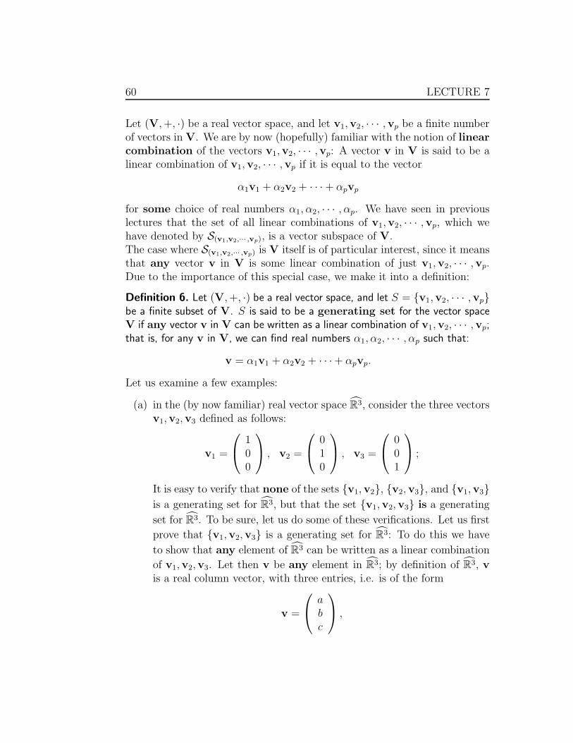
(a) in the (by now familiar) real vector space R3, consider the three vectorsv1,v2,v3 defined as follows:
v1 =
100
, v2 =
010
, v3 =
001
;
It is easy to verify that none of the sets {v1,v2}, {v2,v3}, and {v1,v3}is a generating set for R3, but that the set {v1,v2,v3} is a generating
set for R3. To be sure, let us do some of these verifications. Let us first
prove that {v1,v2,v3} is a generating set for R3: To do this we have
to show that any element of R3 can be written as a linear combination
of v1,v2,v3. Let then v be any element in R3; by definition of R3, vis a real column vector, with three entries, i.e. is of the form
v =
abc
,

61
for some real numbers a, b and c; but then, it is clear that we have theequality
v = av1 + bv2 + cv3,
since, writing it out in detail, we have:
av1 + bv2 + cv3 = a
100
+ b
010
+ c
001
=
a00
+
0b0
+
00c
=
abc
,
which is none other than v. This proves our assertion that any element
in R3 can be written as a linear combination of v1,v2,v3, and hence
shows that {v1,v2,v3} is indeed a generating set for R3.
Let us now show that {v1,v2} is not a generating set for R3; for this it
is enough to find one vector in R3 which cannot be written as a linear
combination of v1 and v2; consider then the vector v in R3 defined by:
v =
001
Let us show there is no linear combination of v1 and v2 that equalsv. How can we show this ? Well, we can assume that there doesexist such a linear combination, and show that we are then led to acontradiction. Let us then assume that there do exist real numbersα1, α2 such that
v = α1v1 + α2v2,
or, equivalently,
001
= α1
100
+ α2
010
,

62 LECTURE 7
that is,
001
=
α1
00
+
0α2
0
=
α1
α2
0
;
But we have a contradiction since the two column vectors
001
and
α1
α2
0
can never be equal, no matter what α1 and α2 are (since
their equality would imply that 1 = 0). This shows that there is nolinear combination of v1 and v2 that equals v; hence, {v1,v2} is not
a generating set for R3.
(b) Consider now the (equally familiar) real vector space R2 of all realcolumn vectors with two entries. Consider the subset S = {v1,v2,v3}of R2, where the vectors v1,v2,v3 in R2 are defined as:
v1 =
(10
), v2 =
(01
), v3 =
(−1
0
).
Let us show that S = {v1,v2,v3} is a generating set for R2. To do
this, we have to show that any element in R2 can be written as a linear
combination of v1,v2,v3. Let then
(ab
)(with a, b real numbers) be
any element of R2; it is clear that we can write:(
ab
)= av1 + bv2 + 0v3,
that is, any element
(ab
)of R2 can be written as a linear combination
of v1,v2,v3. This shows that S is indeed a generating set for R2.
Let us note now that
(ab
)can also be expressed as the following
linear combination of v1,v2,v3:(
ab
)= 0v1 + bv2 − av3,
63
and even as the following linear combination:(
ab
)= 2av1 + bv2 + av3,
and even as:(
ab
)= 3av1 + bv2 + 2av3,
and so on ... (you get the idea). This shows that any element in R2
can be written as many distinct linear combinations of v1,v2,v3.
The case where a given generating set of a vector space is such that any vectorin that vector space can be expressed as a linear combination of vectors in thegenerating set in a unique way is of particular interest, since then there is noambiguity as to how the vector should be written as a linear combination ofthe elements of the generating set. Note that this was the case with Example(a) above (prove it!), but not with Example (b).A very natural question at this point is therefore the following: Suppose wehave a vector space V, and we are given a finite subset S of V which is alsoa generating set for V. We then know of course that any element of Vcan be written as some linear combination of the elements of S; how then,can we determine whether that is the only possible linear combination thatyields the desired element ? We already have the answer to that questionfrom Theorem 4 of Lecture 6; we can therefore state:
Theorem 8. Let (V, +, ·) be a real vector space, and let S = {v1, · · · ,vp} bea finite subset of V such that:
(i) S is a generating set for V, and
(ii) S is a linearly independent of V;
Then, any element of V can be expressed in a unique way as a linear combi-nation of elements of S.
Finite subsets of V which happen to be both generating and linearly inde-pendent are of particular importance, as we will see later; we shall thereforegive them a special name. However, for a reason that will become clear soon,we will care about the order, i.e. we will consider not just subsets ofV, but rather ordered subsets, or equivalently p−tuples of vectors. Wetherefore define:
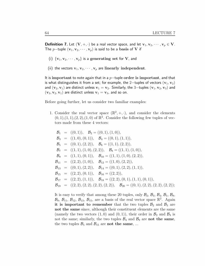
64 LECTURE 7
Definition 7. Let (V, +, ·) be a real vector space, and let v1,v2, · · · ,vp ∈ V.The p−tuple (v1,v2, · · · ,vp) is said to be a basis of V if
(i) {v1,v2, · · · ,vp} is a generating set for V, and
(ii) the vectors v1,v2, · · · ,vp are linearly independent.
It is important to note again that in a p−tuple order is important, and thatis what distinguishes it from a set; for example, the 2−tuples of vectors (v1,v2)and (v2,v1) are distinct unless v1 = v2. Similarly, the 3−tuples (v1,v2,v3) and(v3,v2,v1) are distinct unless v1 = v3, and so on.
Before going further, let us consider two familiar examples:
1. Consider the real vector space (R2, +, ·), and consider the elements(0, 1),(1, 1),(2, 2),(1, 0) of R
2. Consider the following few tuples of vec-tors made from these 4 vectors:
B1 = ((0, 1)), B2 = ((0, 1), (1, 0)),
B3 = ((1, 0), (0, 1)), B4 = ((0, 1), (1, 1)),
B5 = ((0, 1), (2, 2)), B6 = ((1, 1), (2, 2)),
B7 = ((1, 1), (1, 0), (2, 2)), B8 = ((1, 1), (1, 0)),
B9 = ((1, 1), (0, 1)), B10 = ((1, 1), (1, 0), (2, 2)),
B11 = ((2, 2), (1, 0)), B12 = ((1, 0), (2, 2)),
B13 = ((0, 1), (2, 2)), B14 = ((0, 1), (2, 2), (1, 1)),
B15 = ((2, 2), (0, 1)), B16 = ((2, 2)),
B17 = ((2, 2), (1, 1)), B18 = ((2, 2), (0, 1), (1, 1), (0, 1)),
B19 = ((2, 2), (2, 2), (2, 2), (2, 2)), B20 = ((0, 1), (2, 2), (2, 2), (2, 2));
It is easy to verify that among these 20 tuples, only B2, B3, B4, B5, B8,B9, B11, B12, B13, B15, are a basis of the real vector space R
2. Againit is important to remember that the two tuples B2 and B3 arenot the same since, although their constituent elements are the same(namely the two vectors (1, 0) and (0, 1)), their order in B2 and B3 isnot the same; similarly, the two tuples B4 and B9 are not the same,the two tuples B5 and B15 are not the same, ...

65
2. Consider the real vector space (R3, +, ·), and consider the vectors
v1 =
100
,v2 =
010
,v3 =
001
,
v4 =
110
,v5 =
111
,v6 =
011
,
of R3. Here again, it is easy to verify that each of the 3−tuples(v1,v2,v3),(v2,v1,v3),(v3,v1,v2),(v1,v2,v6),(v6,v2,v1) (and still many
more!) are distinct bases of the real vector space R3; on the other hand,the tuples (v1), (v1,v2), (v3), (v1,v1,v1), (v5,v6) (to give only a few
examples) do not form a basis of R3.
The attentive reader may have noticed that in the case of the real vectorspace R
2 given above, all the tuples which did form a basis of R2 happened
to have exactly the same number of vectors (namely 2); similarly, in the
case of the real vector space R3, all the tuples which did form a basis of R3
happened to have exactly the same number of vectors (namely 3). We willsee in the next lecture that this is not accidental, and that in a vector space,all bases have the same number of elements.Now that we have defined the notion of basis for a real vector space, wedefine another important notion, that of components of a vector withrespect to a basis:
Definition 8. Let (V, +, ·) be a real vector space, let B = (v1,v2, · · · ,vp) bea basis of V, and let v ∈ V. The p−tuple (α1, α2, · · · , αp) of real numbersis called the component vector or coordinate vector of v with respect tothe basis B if we have:
α1v1 + α2v2 + · · · + αpvp = v.
The real number α1 is called the first component (or first coordinate) of v withrespect to the basis B, the real number α2 is called the second component (orsecond coordinate) of v with respect to the basis B, ... and so on.
It is absolutely essential to note the following point:

66 LECTURE 7
• If B = (v1,v2, · · · ,vp) is a basis of V and v is an element of V,then v has at least one component vector with respect to B (since{v1,v2, · · · ,vp} is a generating set for V); furthermore, since the vec-tors v1,v2, · · · ,vp are linearly independent, there is only a uniquep−tuple (α1, · · · , αp) of real numbers for which α1v1+α2v2+· · ·+αpvp
is equal to v; i.e. to each v in V there corresponds only a unique com-ponent vector. This is why in the previous definition, we wrote “thecomponent vector of v with respect to B” and not “a component vectorof v with respect to B”.
It is also important to make note of the following point:
• If B = (v1,v2, · · · ,vp) is a basis of V and v is an element of V, we havedefined the component vector of v with respect to B to be some p−tupleof real numbers, i.e. some element of R
p; we will find it occasionallyconvenient to denote the component vector of v by an element of Rp
instead, i.e. by a column vector with p real entries.
We close this section with three examples:
(a) Consider the real vector space (R2+, ·), and let W denote the subsetof R
2 consisting of all pairs (x, y) of real numbers such that x = y.It is easy to verify that W is a vector subspace of R
2, and hence, byProblem 4 of Lecture 3, W (with the operations of addition and scalarmultiplication it receives from R
2) is itself a real vector space. Considerthe vector v1 = (1, 1) of R
2; clearly, v1 is an element of W, since W isthe subset of R
2 consisting of all pairs (x, y) with x = y, and the pair(1, 1) satisfies this condition. Consider the “1−tuple” B = (v1); let usshow that B is a basis of W. To do this, we have to show two things:
(i) That {v1} is a generating set for W, and
(ii) that {v1} is a linearly independent subset of W.
To show (i), namely that {v1} is a generating set for W, we have toshow that any v ∈ W can be written as some linear combination of v1;let then v = (x, y) be an element of W; since (x, y) is in W, we have(by definition of W) x = y. Hence, v = (x, x) = x(1, 1) = xv1, whichshows that v is a linear combination of v1. To recapitulate, we haveshown that any element of W is a linear combination of v1; this proves
67
that {v1} is a generating set for W. Let us now show (ii), i.e. that {v1}is a linearly independent set. Let then α be any real number such thatαv1 = 0; we have to show that we must then have α = 0. Now, αv1 = 0is equivalent to α(1, 1) = (0, 0), which is equivalent to (α, α) = (0, 0),which implies α = 0. Hence, we have shown that αv1 = 0 impliesα = 0, and this proves that {v1} is a linearly independent subset ofW. We have thus shown (i) and (ii), and hence, we have shown thatB is a basis of W.
Any element of W is a pair of the form (a, a) for some a ∈ R; Let uscompute the component vector of (a, a) with respect to the basis B.We have:
(a, a) = a(1, 1) = av1,
which shows that the component vector of the vector (a, a) of W withrespect to the basis B is the 1−tuple (a). (Note: It may sound a bitakward to talk about 1−tuples, but think of them as a list with onlyone entry!).
(b) Consider the real vector space (R3, +, ·), and let v1 = (1, 0, 0), v2 =(0, 1, 0), v3 = (0, 0, 1), v4 = (1, 1, 0), v5 = (1, 1, 1). It is easy to verifythat each of the 3−tuples of vectors B1 = (v1,v2,v3), B2 = (v2,v3,v1),and B3 = (v1,v4,v5) is a basis of R
3. Let now v = (a, b, c) be anelement of R
3. It is easy to verify that the component vector of v withrespect to B1 is (a, b, c) (i.e. v itself!), whereas its component vectorwith respect to the basis B2 is (b, c, a), and its component vector withrespect to the basis B3 is (a − b, b − c, c).
(c) Consider again the real vector space (R3, +, ·), and let W be the subsetof R
3 consisting of all triples (x, y, z) with x + y + z = 0. It is easy toverify that W is a vector subspace of R
3. By Problem 4 of Lecture 3, weknow that W (with the operations of addition and scalar multiplicationit receives from R
3) is itself a real vector space. Consider the elementsv1,v2 of W defined by:
v1 = (1, 0,−1),
v2 = (0, 1,−1).
Define B to be the 2−tuple B = (v1,v2). Let us show that B is indeeda basis for the real vector space W. Once again, to show this, we mustshow two things:

68 LECTURE 7
(i) That {v1,v2} is a generating set for W, and
(ii) that {v1,v2} is a linearly independent subset of W.
Let us first show (i): We have to show that any element of W is somelinear combination of v1 and v2. Let then v = (x, y, z) be any elementin W. Since v is in W, we must have (by definition of W) x+y+z = 0,i.e. z = −x − y. Hence, v = (x, y,−x − y). Now note that we canwrite:
v = (x, y,−x − y)
= (x, 0,−x) + (0, y,−y)
= x(1, 0,−1) + y(0, 1,−1)
= xv1 + yv2,
which shows that v is a linear combination of v1 and v2. We have thusshown that any element of W is a linear combination of v1 and v2,and this shows that {v1,v2} is a generating set for W.
Let us now show (ii). Let then α, β be real numbers such that αv1 +βv2 = 0; we must show that this necessarily implies that α = β = 0.Now, αv1 + βv2 = 0 is equivalent to
α(1, 0,−1) + β(0, 1,−1) = (0, 0, 0),
which is equivalent to
(α, 0,−α) + (0, β,−β) = (0, 0, 0),
which is equivalent to
(α, β,−α − β) = (0, 0, 0),
which implies α = β = 0. Hence, we have shown that if α, β are realnumbers such that αv1 + βv2 = 0 then it must follow that α = β = 0.This proves (ii), i.e. that {v1,v2} is a linearly independent subsetof W. We have therefore shown (i) and (ii), i.e., we have shown thatB is a basis of W.
Let now (a, b, c) be any element of W; let us compute the componentvector of (a, b, c) with respect to the basis B. Since (a, b, c) is in W, we
69
must have (by definition of W) a+b+c = 0; it follows that c = −a−b,i.e.
(a, b, c) = (a, b,−a − b) = a(1, 0,−1) + b(0, 1,−1) = av1 + bv2,
which shows that the component vector of the element (a, b, c) of Wwith respect to the basis B is the pair (a, b).
PROBLEMS:
1. Consider the real vector space (R3, +, ·), and consider the followingvectors in R
3:
v1 = (1, 0, 0), v2 = (1, 1, 0), v3 = (1, 2, 1), v4 = (0, 0, 3),
(a) Show that {v1} is not a generating set for R3.
(b) Show that {v2} is not a generating set for R3.
(c) Show that {v3} is not a generating set for R3.
(d) Show that {v4} is not a generating set for R3.
(e) Show that {v1,v2} is not a generating set for R3.
(f) Show that {v1,v3} is not a generating set for R3.
(g) Show that {v2,v3} is not a generating set for R3.
(h) Show that {v1,v4} is not a generating set for R3.
(i) Show that {v1,v2,v3} is a generating set for R3.
(j) Show that {v1,v2,v4} is a generating set for R3.
(k) Show that {v1,v3,v4} is a generating set for R3.
(l) Show that {v2,v3,v4} is a generating set for R3.
(m) Show that {v1,v2,v3,v4} is a generating set for R3.
2. Consider the real vector space (R3, +, ·), and let W be the subset of
R3 consisting of all elements
xyz
of R3 for which x + y − z = 0. It

70 LECTURE 7
is easy to verify that W is a vector subspace of R3, and hence, is itselfa real vector space.
Consider now the following vectors in W:
v1 =
101
, v2 =
022
, v3 =
1
−10
, v4 =
000
.
(a) Show that {v1} is not a generating set for W.
(b) Show that {v2} is not a generating set for W.
(c) Show that {v3} is not a generating set for W.
(d) Show that {v4} is not a generating set for W.
(e) Show that {v1,v4} is not a generating set for W.
(f) Show that {v2,v4} is not a generating set for W.
(g) Show that {v3,v4} is not a generating set for W.
(h) Show that {v1,v2} is a generating set for W.
(i) Show that {v2,v3} is a generating set for W.
(j) Show that {v1,v3} is a generating set for W.
(k) Show that {v1,v2,v3} is a generating set for W.
(l) Show that {v1,v2,v3,v4} is a generating set for W.
3. Consider the real vector space (R4, +, ·), and let W be the subset ofR
4 consisting of all 4−tuples (x, y, z, w) of real numbers for which 3x+y − w = 0 and z − 2w = 0. It is easy to verify that W is a vectorsubspace of W, and hence, is itself a real vector space. Consider thefollowing vectors in W:
v1 = (1, 0, 6, 3), v2 = (0, 1, 2, 1), v3 = (1, 1, 8, 4)
(a) Show that {v1} is not a generating set for W.
(b) Show that {v2} is not a generating set for W.
(c) Show that {v3} is not a generating set for W.
(d) Show that {v1,v2} is a generating set for W.
(e) Show that {v1,v3} is a generating set for W.

71
(f) Show that {v2,v3} is a generating set for W.
(g) Show that {v1,v2,v3} is a generating set for W.
4. Consider the real vector space (R2, +, ·), and consider the followingvectors in R
2:
v1 = (1, 1), v2 = (−1, 1), v3 = (0, 1), v4 = (1, 2)
(a) Show that (v1) is not a basis of R2.
(b) Show that (v2) is not a basis of R2.
(c) Show that (v3) is not a basis of R2.
(d) Show that (v4) is not a basis of R2.
(e) Show that B1 = (v1,v2) is a basis of R2.
(f) Show that B2 = (v1,v3) is a basis of R2.
(g) Show that B3 = (v1,v4) is a basis of R2.
(h) Show that B4 = (v2,v3) is a basis of R2.
(i) Show that B5 = (v3,v2) is a basis of R2.
(j) Show that B6 = (v3,v4) is a basis of R2.
(k) Show that (v1,v2,v3) is not a basis of R2.
(l) Show that (v1,v2,v4) is not a basis of R2.
(m) Show that (v1,v2,v3,v4) is not a basis of R2.
(n) Compute the component vectors of v1 with respect to each of thebases B1, · · · ,B6.
(o) Compute the component vectors of v2 with respect to each of thebases B1, · · · ,B6.
(p) Compute the component vectors of v3 with respect to each of thebases B1, · · · ,B6.
(q) Compute the component vectors of v4 with respect to each of thebases B1, · · · ,B6.
5. Consider the real vector space (R4, +, ·), and let W be the subset ofR
4 consisting of all 4−tuples (x, y, z, w) of real numbers for which x +y + z − w = 0 and y − z = 0. It is easy to verify that W is a vector

72 LECTURE 7
subspace of R4, and hence, is itself a real vector space. Consider the
following vectors in W:
v1 = (1, 0, 0, 1), v2 = (0, 1, 1, 2), v3 = (1, 1, 1, 3), v4 = (1,−1,−1,−1).
(a) Show that (v1) is not a basis of W.
(b) Show that (v2) is not a basis of W.
(c) Show that (v3) is not a basis of W.
(d) Show that (v4) is not a basis of W.
(e) Show that B1 = (v1,v2) is a basis of W.
(f) Show that B2 = (v1,v3) is a basis of W.
(g) Show that B3 = (v3,v1) is a basis of W.
(h) Show that B4 = (v1,v4) is a basis of W.
(k) Show that (v1,v2,v3) is not a basis of W.
(l) Show that (v1,v2,v4) is not a basis of W.
(m) Show that (v1,v3,v4) is not a basis of W.
(n) Compute the component vectors of v1 with respect to each of thebases B1, · · · ,B4.
(o) Compute the component vectors of v2 with respect to each of thebases B1, · · · ,B4.
(p) Compute the component vectors of v3 with respect to each of thebases B1, · · · ,B4.
(q) Compute the component vectors of v4 with respect to each of thebases B1, · · · ,B4.

Lecture 8
Study Topics
• Finite-dimensional vector spaces
• Dimension of a real vector space
73
74 LECTURE 8
We know from elementary geometry that we can represent real numbers (i.e.elements of the real vector space R) by points on a line, pairs of real numbers(i.e. elements of the real vector space R
2) by points in a plane, triples of realnumbers (i.e. elements of the real vector space R
3) by points in space, ...The question we may ask at this point is how the difference between, say,a line and a plane, manifests itself in a difference between the vector spacesR and R
2. Or how the difference between a plane and space manifests itselfin a difference between the vector spaces R
2 and R3. In other words, how is
the “line-like” feature of the real vector space R captured in the vector spacestructure of R, how is the “plane-like” feature of the real vector space R
2
captured in the vector space structure of R2, how is the “space-like” feature
of the real vector space R3 captured in the vector space structure of R
3, ...In one word: How do these “geometric” concepts get expressed in terms oflinear algebra ? We shall soon see that one point of contact between linearalgebra and geometry is given by the notion of dimension.
Definition 9. Let (V, +, ·) be a real vector space.
• V is said to be finite-dimensional if there exists an integer N ≥ 0 suchthat any subset of V containing N +1 elements is linearly dependent.The smallest integer N for which this holds is then called the dimensionof V (equivalently, V is said to have dimension N).
• V is said to be infinite-dimensional if it is not finite-dimensional.
It is important to note the following points:
• By the above definition, if V has dimension N , then any subset ofV containing N + 1 elements is linearly dependent, and as a result,any subset of V containing N + 2 or more elements is also linearlydependent.
• By the above definition, if V has dimension N , then any subset of Vcontaining N + 1 elements is linearly dependent, but there exists atleast one linearly independent subset of V containing exactly Nelements, since otherwise the dimension of V would be strictly lessthan N .
• V is infinite-dimensional if for any positive integer N , no matterhow large, there exists a linearly independent subset of V containingexactly N elements.

75
Let’s recapitulate:
• V is said to have dimension N if and only if the following two conditionsare met:
(i) There exists a linearly independent subset of V containing ex-actly N elements,
(ii) Any subset of V containing N + 1 elements is linearly depen-dent.
Let us now examine some simple examples:
1. Recall the real vector space (F(R; R), +, ·) consisting of all functionsf : R → R (i.e. all real-valued functions of a real variable). Let us showthat F(R; R) is an infinite-dimensional vector space. To do this, wehave to show that for any integer N ≥ 0 (no matter how large), thereexists a linearly independent subset of F(R; R) containing exactlyN elements.
Let then N be any integer ≥ 0. Consider the following elementsf1, f2, · · · , fN in F(R; R) defined as follows:
f1(t) = 0 for t 6= 1 and f1(1) = 1,
f2(t) = 0 for t 6= 2 and f2(2) = 1,
f3(t) = 0 for t 6= 3 and f3(3) = 1,
· · ·fN(t) = 0 for t 6= N and fN (N) = 1.
(You may want to draw the graphs of these functions just to see whatthey look like). In other words, if k is an integer in the range 1 ≤ k ≤ N ,fk is the function from R to R defined to be 0 everywhere except atk (where it takes the value 1). Let us show that {f1, f2, · · · , fN} is alinearly independent subset of F(R; R). Let then α1, α2, · · · , αN bereal numbers such that
α1f1 + α2f2 + · · ·+ αNfn = 0.
(Recall that the zero vector 0 of the vector space F(R; R) is the functionfrom R to R which maps every real number to zero). We have to show
76 LECTURE 8
that α1,α2,· · · ,αN must all be zero. Now, the equality
α1f1 + α2f2 + · · · + αNfn = 0.
is equivalent to
α1f1(t) + α2f2(t) + · · ·+ αNfn(t) = 0, ∀t ∈ R,
and in particular, this last equality must hold for particular choicesof t, such as t = 1, t = 2, · · · , t = N . But since f1(1) = 1 andf2(1) = f3(1) = · · · = fN(1) = 0, the above equality, for the particularchoice of t = 1 becomes:
α1 = 0.
Similarly, since f2(2) = 1 and f1(2) = f3(2) = · · · = fN(2) = 0, thatsame equality, for the particular choice of t = 2 becomes:
α2 = 0.
Continuing in this way with, successively, t = 3, t = 4, · · · , t = N , weobtain successively that α3 = 0, α4 = 0, · · · , αN = 0. Hence, we haveshown that if α1, α2, · · · , αN are real numbers such that
α1f1 + α2f2 + · · · + αNfn = 0,
then it follows that α1 = α2 = · · · = αN = 0. This proves that{f1, f2, · · · , fN} is a linearly independent subset of F(R; R).
Let us recapitulate: For any integer N ≥ 0, we have constructeda linearly independent subset of F(R; R) containing exactly Nelements; this proves that F(R; R) is an infinite-dimensional realvector space.
2. Let V be a set containing only one element, which we denote by ξ (thezero vector), that is, V = {ξ}; define addition and scalar multiplicationon V as follows:
ξ + ξ = ξ
α · ξ = ξ, ∀α ∈ R.

77
It is easy to verify that (V, +, ·) is a real vector space and that ξ itself isthe zero vector of this vector space. Let us show that V has dimension0. Let N = 0; there is only one possible subset of V containing N +1 = 1 elements, namely {ξ}, which is V itself, and since that subsetcontains the zero vector (since ξ itself is the zero vector), that subsetis linearly dependent. It follows from the definition of dimension thatV is 0−dimensional.
3. Let now V = R, with the usual addition and multiplication operations(we have already seen that with these operations, R is a real vectorspace). Let us show that V has dimension 1. For this, we have toshow that we can find a linearly independent subset of R containingexactly one element, but that any subset of R containing two elementsis linearly dependent. Consider then the subset of R given by {1} (i.e.the subset containing only the vector 1 of R). Let α ∈ R, and assumeα · 1 = 0; since α · 1 = α, this implies α = 0, which shows that {1} is alinearly independent subset of R. Let us now show that any subset ofR containing two elements is linearly dependent. Let then {v1,v2} beany subset of R; we have to show that there exists a linear combinationαv1 + βv2 of v1,v2 that is equal to 0 but such that α, β are not bothzero. Consider the following three cases:
(i) If v1 = 0, then with α = 1, β = 0, we obtain αv1 + βv2 = 0,and since α, β are not both zero (since α = 1), this proves lineardependence of {v1,v2} in this case.
(ii) If v2 = 0, then with α = 0, β = 1, we obtain αv1 + βv2 = 0,and since α, β are not both zero (since β = 1), this proves lineardependence of {v1,v2}.
(iii) If v1 6= 0 and v2 6= 0, then, with α = 1, β = −v1
v2
(remember thatsince V = R in this example, our vectors are real numbers so wecan divide by them if they are non-zero), we have αv1 + βv2 = 0,and since α, β are not both zero, this proves linear dependence of{v1,v2}.
Hence, we have linear dependence of {v1,v2} in all cases. To recapit-ulate, we have shown that:
• There exists a linearly independent subset of R containing exactlyone element,

78 LECTURE 8
• Any subset of R containing two elements is linearly dependent.
This proves that R has dimension 1.
The reader may feel at this point that the dimension of a real vector spacemay not be such an easy thing to compute: After all, it took us quite a fewlines above to compute the dimension of a simple vector space such as R.Recall again that to prove that a real vector space has dimension N , we haveto do two things:
• Find N linearly independent vectors in that vector space,
• Show that any subset containing N + 1 vectors is linearly dependent.
The first item is usually easy to accomplish; it is enough to find one linearlyindependent subset containing exactly N elements. The difficulty comesfrom the second item: How does one prove that any subset containing N +1elements is necessarily linearly dependent ?The following theorems will yield an extremely simple way to compute thedimension of a finite-dimensional real vector space.
Theorem 9. Let (V, +, ·) be a finite-dimensional real vector space of di-mension N . Let {v1, · · · ,vp} be a finite subset of V containing p vectors. If{v1, · · · ,vp} is a linearly independent subset of V then p ≤ N .
Proof. The proof follows directly from the definition of dimension. If we hadp > N , then that would mean that p ≥ N + 1; since V is assumed to havedimension N , we know (by definition of dimension) that any subset of Vcontaining N + 1 or more elements has to be linearly dependent; hence, ifp > N , i.e. equivalently p ≥ N + 1, the subset {v1, · · · ,vp} has N + 1 ormore elements, and hence is linearly dependent. Hence, if we assume that{v1, · · · ,vp} is linearly independent, then we must have p ≤ N .
Theorem 10. Let (V, +, ·) be a finite-dimensional real vector space of di-mension N . Let {v1, · · · ,vp} be a finite subset of V containing p vectors. If{v1, · · · ,vp} is a generating set for V of V then p ≥ N .
Proof. We will show that, under the assumption that {v1, · · · ,vp} is a gen-erating set for V, we cannot have p < N . So let us begin by assuming that{v1, · · · ,vp} is a generating set for V, and that p < N ; we will show thatthis leads to a contradiction.
79
Since V is assumed to have dimension N , there does exist (by definition ofdimension) a linearly independent subset of V containing exactly N ele-ments; let {e1, · · · , eN} denote that subset. Since {v1, · · · ,vp} is a generat-ing set for V, each of e1, e2, · · · , eN can be expressed as a linear combinationof v1, · · · ,vp. Let us start with e1; we can write:
e1 = α1v1 + α2v2 + · · · + αpvp,
for some real numbers α1, α2, · · · , αp. Since the subset {e1, · · · , eN} is lin-early independent, none of e1, · · · , eN is the zero vector; in particular,e1 6= 0, and hence, at least one of α1, α2, · · · , αp must be non-zero (sinceif all of α1, α2, · · · , αp were zero, we would obtain e1 = 0 from the linearcombination above). Assume with no loss of generality (relabel the vectorsif necessary) that it is α1 which is non-zero, i.e. α1 6= 0. We can then write:
v1 =1
α1e1 −
α2
α1v2 − · · · − αp
α1vp,
and this shows that {e1,v2,v3, · · · ,vp} is a generating set for V (since{v1,v2, · · · ,vp} itself is assumed to be a generating set for V). Hence e2 canbe written as some linear combination of e1,v2,v3, · · · ,vp, i.e.
e2 = λ1e1 + λ2v2 + λ3v3 + · · ·+ λpvp,
for some real numbers λ1, · · · , λp. Note that at least one of λ2, λ3, · · · , λp isnon-zero, since if all of λ2, λ3, · · · , λp were zero, we would obtain e2 = λ1e1,contradicting the linear independence of {e1, · · · , eN}. Assume with no lossof generality (relabel the vectors if necessary) that it is λ2 which is non-zero,i.e. λ2 6= 0. This then yields:
v2 = −λ1
λ2
e1 +1
λ2
e2 −λ3
λ2
v3 − · · · − λp
λ2
vp,
This last equality, together with the equality
v1 =1
α1
e1 −α2
α1
v2 − · · · − αp
α1
vp,
and the assumption that {v1,v2, · · · ,vp} is a generating set for V, im-plies that {e1, e2,v3,v4 · · · ,vp} is a generating set for V. Continuining

80 LECTURE 8
in this way, we obtain successively that {e1, e2, e3,v4 · · · ,vp} is a gener-ating set for V, that {e1, e2, e3, e4,v5 · · · ,vp} is a generating set for V,..., and finally, that {e1, e2, e3, · · · , ep} is a generating set for V, in otherwords, that the linear span of {e1, e2, e3, · · · , ep} is the whole vector spaceV. Note that we have assumed p < N ; hence, the number of elementsof {e1, e2, e3, · · · , ep} is strictly smaller than the number of elements of{e1, e2, e3, · · · , ep, ep+1, · · · , eN}. In particular, eN is in the linear span of{e1, e2, e3, · · · , ep}, and this contradicts the assumed linear independenceof {e1, e2, e3, · · · , ep, ep+1, · · · , eN}. Hence, we cannot have p < N ; in otherwords, we must have p ≥ N .
We can now combine the previous two theorems in the following theorem:
Theorem 11. Let (V, +, ·) be a finite-dimensional real vector space of dimen-sion N . Let B = (v1,v2, · · · ,vp) be a basis for V. Then, we must havep = N .
Proof. Since (v1,v2, · · · ,vp) is assumed to be a basis for V, {v1,v2, · · · ,vp}is both a generating subset for V and a linearly independent subset ofV; the first property implies p ≥ N , and the second property implies p ≤ N .Together, they imply p = N .
We can establish the following two very important corollaries of theprevious theorem:
(i) In a finite-dimensional real vector space, all bases have the samenumber of elements (and that number is the dimension of the vectorspace);
(ii) To compute the dimension of a finite-dimensional real vector space,it is enough to find a basis for it; the dimension of the vector spaceis then equal to the number of elements of the basis.
Let us illustrate the application of these results on some examples:
1. Consider the (by now extremely familiar) real vector space (R2, +, ·).Let us compute the dimension of R
2. As we have seen above, all weneed to do is find a basis for R
2; the dimension of R2 will then be equal
to the number of elements of that basis. Consider then the followingvectors in R
2:
v1 = (1, 0), v2 = (0, 1).

81
We have already seen that (v1,v2) is a basis of R2; since it has 2
elements, we conclude that R2 is a real vector space of dimension 2.
2. Consider the (equally familiar) real vector space (R3, +, ·). Let us com-pute the dimension of R
3. As we have seen above, all we need to dois find a basis for R
3; the dimension of R3 will then be equal to the
number of elements of that basis. Consider the following vectors in R3:
v1 = (1, 0, 0), v2 = (0, 1, 0), v3 = (0, 0, 1).
We have already seen that (v1,v2,v3) is a basis of R3; since it has 3
elements, we conclude that R3 is a real vector space of dimension 3.
3. More generally, let n be an integer ≥ 1 and consider the real vectorspace (Rn, +, ·). Let us compute the dimension of R
n. Proceeding asbefore, let us construct a basis for R
n; the dimension of Rn will then
be given by the number of elements in that basis. For this, considerthe following elements of R
n:
v1 = (1, 0, 0, 0, · · · , 0),
v2 = (0, 1, 0, 0, · · · , 0),
v3 = (0, 0, 1, 0, · · · , 0),
· · ·vn = (0, 0, 0, 0, · · · , 1).
(i.e. vk is the n−tuple with the kth entry equal to 1 and all other entriesequal to 0). It is easy to verify that (v1,v2,v3, · · · ,vn) is a basis of R
n.Since it has exactly n elements, this shows that R
n has dimension n.
4. Consider the vector subspace W of R2 defined as the set of all (x, y) in
R2 with x = y. Consider the vector v1 = (1, 1) in W. We have alreadyseen (in the previous lecture) that (v1) is a basis of W. Since it hasone element, we deduce that W is a real vector space of dimension 1.
5. Consider now the vector subspace W of R3 defined as the set of all
(x, y, z) in R3 with x + y + z = 0. Consider the vectors v1 = (1, 0,−1)
and v2 = (0, 1,−1) of W. We have already seen (in the previouslecture) that (v1,v2) is a basis of W. Since it has 2 elements, weconclude that W is a real vector space of dimension 2.

82 LECTURE 8
Let us restate once more the following important point:
• To compute the dimension of a real vector space, it is enough tofind a basis for that vector space. The dimension of the vectorspace is then equal to the number of elements of that basis.
PROBLEMS:
1. Let C(R; R) be the real vector space of all continuous functions from R
to R (with addition and scalar multiplication defined as in F(R; R)).Show that C(R; R) is an infinite-dimensional vector space.
2. Consider the vector subspace W of R2 defined as the set of all (x, y) ∈
R2 such that x + y = 0. Show that W has dimension 1.
3. Consider the vector subspace W of R2 defined as the set of all (x, y) ∈
R2 such that 2x + 3y = 0. Show that W has dimension 1.
4. Consider the vector subspace W of R2 defined as the set of all (x, y) ∈
R2 such that 5x − 7y = 0. Show that W has dimension 1.
5. Consider the vector subspace W of R2 defined as the set of all (x, y) ∈
R2 such that x = 0. Show that W has dimension 1.
6. Consider the vector subspace W of R2 defined as the set of all (x, y) ∈
R2 such that y = 0. Show that W has dimension 1.
7. Consider the vector subspace W of R3 defined as the set of all (x, y, z) ∈
R3 such that x − y = 0. Show that W has dimension 2.
8. Consider the vector subspace W of R3 defined as the set of all (x, y, z) ∈
R3 such that 2x + y + z = 0. Show that W has dimension 2.
9. Consider the vector subspace W of R3 defined as the set of all (x, y, z) ∈
R3 such that x = 0. Show that W has dimension 2.
10. Consider the vector subspace W of R3 defined as the set of all (x, y, z) ∈
R3 such that y = 0. Show that W has dimension 2.
83
11. Consider the vector subspace W of R3 defined as the set of all (x, y, z) ∈
R3 such that z = 0. Show that W has dimension 2.
12. Consider the vector subspace W of R3 defined as the set of all (x, y, z) ∈
R3 such that x + y = 0 and z = 0. Show that W has dimension 1.
13. Consider the vector subspace W of R3 defined as the set of all (x, y, z) ∈
R3 such that x−z = 0 and x+y +z = 0. Show that W has dimension
1.
14. Consider the vector subspace W of R4 defined as the set of all (x, y, z, w) ∈
R4 such that x + y + z + w = 0. Show that W has dimension 3.
15. Consider the vector subspace W of R4 defined as the set of all (x, y, z, w) ∈
R4 such that x + w = 0. Show that W has dimension 3.
16. Consider the vector subspace W of R4 defined as the set of all (x, y, z, w) ∈
R4 such that x − y = 0. Show that W has dimension 3.
17. Consider the vector subspace W of R4 defined as the set of all (x, y, z, w) ∈
R4 such that x = 0. Show that W has dimension 3.
18. Consider the vector subspace W of R4 defined as the set of all (x, y, z, w) ∈
R4 such that w = 0. Show that W has dimension 3.
19. Consider the vector subspace W of R4 defined as the set of all (x, y, z, w) ∈
R4 such that x+ y = 0 and z +w = 0. Show that W has dimension 2.
20. Consider the vector subspace W of R4 defined as the set of all (x, y, z, w) ∈
R4 such that x + y + z + w = 0 and z − w = 0. Show that W has
dimension 2.
21. Consider the vector subspace W of R4 defined as the set of all (x, y, z, w) ∈
R4 such that x+2w = 0 and 2z +w = 0. Show that W has dimension
2.
22. Consider the vector subspace W of R4 defined as the set of all (x, y, z, w) ∈
R4 such that x − y = 0 and z + w = 0 and y + w = 0. Show that W
has dimension 1.

84 LECTURE 8
23. Consider the vector subspace W of R4 defined as the set of all (x, y, z, w) ∈
R4 such that x + 2y + z = 0 and z = 0 and 2y + w = 0. Show that W
has dimension 1.
24. Consider the vector subspace W of R4 defined as the set of all (x, y, z, w) ∈
R4 such that x + 2y + z + w = 0 and x + y = 0 and y − z = 0. Show
that W has dimension 1.

Lecture 9
Study Topics
• Linear Transformations
• Range and Kernel of a Linear Transformation
85

86 LECTURE 9
In the previous lectures, we have studied vector spaces by themselves; forexample, we have started from a real vector space, and we have found sub-spaces of that vector space, generating sets for that vector space, linearlydependent or independent subsets for that vector space, bases for that vec-tor space, ... and so on. We now consider functions between vectorspaces, i.e. functions from one vector space to another. Among these func-tions, there are some which have a desirable property (called linearity) whichwe will precisely define shortly; these functions are called linear, and are themain object of study of this and the next few lectures.
A WORD ON TERMINOLOGY: We will often use the words mappingand transformation instead of function – They will all mean the samething.
Definition 10. Let V and W be two real vector spaces, and let L : V → Wbe a mapping from V to W. L is said to be a linear mapping (also called alinear transformation or a linear function) if the following two propertiesare verified:
1. For any v1,v2 ∈ V, L(v1 + v2) = L(v1) + L(v2);
2. For any α ∈ R and any v ∈ V, L(αv) = αL(v).
Before going further, let us give some examples of linear mappings:
1. Let V be a real vector space, and let L : V → V be the identitymapping of V, defined by L(v) = v for all v ∈ V; it is easy to verifythat L is a linear mapping.
2. Let V be a real vector space, let α ∈ R be any real number, and letL : V → V be the mapping defined by L(v) = αv for all v ∈ V; it iseasy to verify that L is a linear mapping.
3. Let V and W be real vector spaces, and let 0W denote the zero vectorof W. Let L : V → W denote the zero mapping from V to W,defined by L(v) = 0W for all v ∈ V (i.e. everything in V is mapped tothe zero vector of W); here again, it is easy to verify that L is a linearmapping.
4. Consider the familiar vector spaces R2 and R, and let L : R
2 → R bethe mapping defined by L((x, y)) = 2x + 3y for all (x, y) ∈ R
2. Let usshow that L is a linear mapping:
87
(i) Let v1 = (x1, y1) ∈ R2 and v2 = (x2, y2) ∈ R
2. We have to showthat L(v1 + v2) = L(v1) + L(v2). We have:
L(v1 + v2) = L((x1, y1) + (x2, y2))
= L((x1 + x2, y1 + y2))
= 2(x1 + x2) + 3(y1 + y2)
= (2x1 + 3y1) + (2x2 + 3y2)
= L((x1, y1)) + L((x2, y2))
= L(v1) + L(v2),
which shows that the first property of a linear mapping is verified.
(ii) Let v = (x, y) ∈ R2 and α ∈ R. We have to show that L(αv) =
αL(v). We have:
L(αv) = L(α(x, y))
= L((αx, αy))
= 2(αx) + 3(αy)
= α(2x + 3y)
= αL((x, y))
= αL(v),
which shows that the second property of a linear mapping is ver-ified.
Both defining properties of a linear mapping are verified; we have there-fore shown that the mapping L of this example is a linear mapping.
5. Consider the familiar real vector spaces R2 and R
3, and let L : R2 → R
3
be the mapping defined by L((x, y)) = (x − y, x + y, 2x + 5y) for all(x, y) ∈ R
2. It is easy to verify that L is a linear mapping.
6. Consider again the familiar real vector spaces R2 and R
3, and let L :R
2 → R3 be the mapping defined by L((x, y)) = (x, y, 0) for all (x, y) ∈
R2. It is easy to verify that L is a linear mapping.
7. Consider once more the familiar real vector spaces R2 and R
3, and letL : R
3 → R2 be the mapping defined by L((x, y, z)) = (x, y) for all
(x, y, z) ∈ R3. It is easy to verify that L is a linear mapping.

88 LECTURE 9
8. Consider now the familiar real vector spaces R3 and R, and let L :
R3 → R be the mapping defined by L((x, y, z)) = x + y + z for all
(x, y, z) ∈ R3. It is easy to verify that L is a linear mapping.
9. Consider now the real vector spaces F(R; R) and R (recall F(R; R)is the real vector space of all functions from R to R), and let L :F(R; R) → R be the mapping defined by L(f) = f(0) for all f ∈F(R; R). Let us prove that L is a linear mapping:
(i) We have to show that ∀f1, f2 ∈ F(R; R), we have L(f1 + f2) =L(f1) + L(f2). We have:
L(f1 + f2) = (f1 + f2)(0)
= f1(0) + f2(0)
= L(f1) + L(f2),
which shows that the first property of a linear mapping is verified.
(ii) Let now f ∈ F(R; R) and α ∈ R; we have to show that L(αf) =αL(f). We have:
L(αf) = (αf)(0)
= αf(0)
= αL(f),
which shows that the second property of a linear mapping is ver-ified.
Both defining properties of a linear mapping are verified; we have there-fore shown that the mapping L of this example is a linear mapping.
10. Consider again the real vector spaces F(R; R) and R, and let L :F(R; R) → R be the mapping defined by L(f) = 5f(1) + 7f(2) forall f ∈ F(R; R). It is easy to verify that L is indeed a linear map-ping.
11. Consider now the real vector spaces C([0, 1]; R) and R, where C([0, 1]; R)denotes the set of all continuous functions from [0, 1] to R (with ad-dition and scalar multiplication defined as for F(R; R); C([0, 1]; R) isactually a vector subspace of F(R; R) (prove it as an exercise!)). De-
fine the mapping L : C([0, 1]; R) → R by L(f) =∫ 1
0f(t)dt, for all
f ∈ C([0, 1]; R). Let us prove that L is a linear mapping:
89
(i) We have to show that ∀f1, f2 ∈ C([0, 1]; R), we have L(f1 + f2) =L(f1) + L(f2). We have:
L(f1 + f2) =
∫ 1
0
(f1 + f2)(t)dt
=
∫ 1
0
(f1(t) + f2(t))dt
=
∫ 1
0
f1(t)dt +
∫ 1
0
f2(t)dt
= L(f1) + L(f2),
which shows that the first property of a linear mapping is verified.
(ii) Let now f ∈ C([0, 1]; R) and α ∈ R; we have to show that L(αf) =αL(f). We have:
L(αf) =
∫ 1
0
(αf)(t)dt
=
∫ 1
0
(αf(t))dt
= α
∫ 1
0
f(t)dt
= αL(f),
which shows that the second property of a linear mapping is ver-ified.
Both defining properties of a linear mapping are verified; we have there-fore shown that the mapping L of this example is a linear mapping.
Before going further and giving examples of mappings between vector spaceswhich are not linear, we prove the following useful and simple theorem:
Theorem 12. Let V and W be real vector spaces; let 0V denote the zero vectorof V, and let 0W denote the zero vector of W. let L : V → W be a linearmapping. Then, we have:
L(0V ) = 0W .
90 LECTURE 9
What the above theorem says, in other words, is the following: if L : V → Wis linear, then it must map the zero vector of V to the zero vector of W.Where can we use this theorem ? Well, if we ever stumble upon a mappingL : V → W which maps the zero vector of V to something other thanthe zero vector of W, then we can be sure that L is not a linear mapping.Before going further, we prove the theorem:
Proof. Let α = 0 (i.e. α is the real number zero); we have α0V = 0V (wehave already shown that any real number times the zero vector is equal tothe zero vector, and in particular if that real number happens to be zero),and therefore, we can write:
L(0V ) = L(α0V )
= αL(0V )
= 0L(0V )
= 0W
since, as we have already shown, the real number 0 times any vector of avector space is equal to the zero vector of that vector space.
Let us now examine mappings between vector spaces, which are not linear.
1. Let V and W be real vector spaces, and let w ∈ W be a given vectorin W such that w 6= 0W (i.e. w is not the zero vector of W). Definethe mapping L : V → W by L(v) = w, for all v ∈ V. We have:
L(0V ) = w 6= 0W ,
i.e. L maps the zero vector of V to something other than the zerovector of W; it follows therefore from the previous theorem that themapping L is not linear.
2. Let V be a real vector space, let λ ∈ R be a real number, and let v1 bea vector in V such that v1 6= 0V (i.e. v1 is distinct from the zero vectorof V). Let L : V → V be the mapping defined by L(v) = λv + v1, forall v ∈ V. We have:
L(0V ) = λ0V + v1
= 0V + v1
= v1 6= 0V ,
91
and since L maps the zero vector of V to something other than the zerovector of V, it follows from the previous theorem that the mapping Lis not linear.
3. Consider the real vector spaces R2 and R, and let L : R
2 → R be themapping defined by L((x, y)) = x2 + y2 for all (x, y) ∈ R
2. Let us showthat the mapping L is not linear. The previous theorem is not of muchhelp here, since L does indeed map the zero vector of R
2 (namely thepair (0, 0)) to the zero vector of R (namely the real number 0); indeed,we have:
L((0, 0)) = 02 + 02 = 0 + 0 = 0;
so we cannot use the previous theorem to show that L is not linear,unlike what we did in the previous examples.
So how do we proceed ? Well, we have to go back to the definition.From there, it is clear that it is enough to find two vectors v1,v2 in R
2
for which L(v1 + v2) is not equal to L(v1) + L(v2), or a real number αand a vector v in R
2 such that L(αv) is not equal to αL(v), in orderto conclude that L is not a linear mapping.
Let us choose for example α = 2 and v = (1, 1). For these choices of αand v, we have:
L(αv) = L(2(1, 1)) = L(2, 2) = 22 + 22 = 4 + 4 = 8,
αL(v) = 2L((1, 1)) = 2(12 + 12) = 2(1 + 1) = 4.
Hence, we have found some real number α (namely α = 2) and somevector v in R
2 (namely v = (1, 1)) for which L(αv) is not equal toαL(v). This shows that the second property in the definition of alinear mapping does not hold for our mapping L, and we concludefrom this that the mapping L is not linear.
4. Consider the real vector space R2, and let L : R
2 → R2 be the mapping
defined by L((x, y)) = (x3 + y, x − y) for all (x, y) ∈ R2. It is easy to
verify here as well that the mapping L defined here is not linear.
5. Consider the real vector space C([0, 1]; R) of all continuous functionsfrom [0, 1] to R, and define the mapping L : C([0, 1]; R) → R fromthe real vector space C([0, 1]; R) to the real vector space R as follows:

92 LECTURE 9
L(f) =∫ 1
0(f(t))2dt for all f ∈ C([0, 1]; R). Let us show that L is not
a linear mapping. For this, let us show that the second property inthe definition of a linear mapping fails in this case. Let then α = 2,and define the vector f ∈ C([0, 1]; R) as follows (recall that in the realvector space C([0, 1]; R), a vector is nothing other than a continuousfunction from [0, 1] to R): f(t) = 1, for all t ∈ R (in other words, f isdefined to be the constant function on [0, 1] which maps every t ∈ [0, 1]to the real number 1). Clearly, f is continuous on [0, 1] with values inR, and hence is an honest element of C([0, 1]; R). With these choicesof α ∈ R and f ∈ C([0, 1]; R), let us compute L(αf) and αL(f). Wehave:
L(αf) =
∫ 1
0
((αf)(t))2dt
=
∫ 1
0
(αf(t))2dt
=
∫ 1
0
α2(f(t))2dt
= α2
∫ 1
0
(f(t))2dt
= 22
∫ 1
0
(1)2dt
= 4
∫ 1
0
dt
= 4,
whereas
αL(f) = α
∫ 1
0
(f(t))2dt
= 2
∫ 1
0
(1)2dt
= 2
∫ 1
0
dt
= 2,
which shows that for these choices of α ∈ R and f ∈ C([0, 1]; R), L(αf)is not equal to αL(f), and this shows that the second property in the

93
definition of a linear mapping does not hold for our mapping L, andwe conclude from this that the mapping L is not linear.
Now that we have seen examples of linear (and non-linear) mappings betweenvector spaces, let us examine an interesting property of linear mappings:Consider three real vector spaces V, W, and Z, let L1 : V → W be amapping from the real vector space V to the real vector space W, andL2 : W → Z a a mapping from the real vector space W to the real vectorspace Z. We know we can then define a mapping from V to Z, which wedenote by L2 ◦ L1 (pay attention to the order!) as follows:
• L2 ◦L1 : V → Z is defined to be the mapping from V to Z which mapsevery element v ∈ V to the element L2(L1(v)) of Z.
L2 ◦ L1 is called the composition of the two mappings L1 and L2; its def-inition is very intuitive: If we are given v in V and we want to computeL2 ◦ L1(v), we first “apply” L1 to v, obtaining the element L1(v) of W.Since L1(v) is in W and since the mapping L2 maps from W (to wher-ever), it makes sense to “apply” L2 to L1(v). We then “apply” L2 to L1(v),obtaining the element of L2(L1(v)) of Z, and it is this last element that wedenote by L2 ◦ L1(v).Let us now again consider three real vector spaces V, W, and Z, let L1 :V → W be a mapping from the real vector space V to the real vector spaceW, and L2 : W → Z a a mapping from the real vector space W to thereal vector space Z; assume now that L1 and L2 are both linear mappings.What can we say then about the mapping L2 ◦ L1 ? The answer is given bythe following theorem:
Theorem 13. Let V, W, and Z be real vector spaces, and let L1 : V → Wand L2 : W → Z be linear mappings. Then, the mapping L2 ◦ L1 : V → Z isalso linear.
Proof. We have to show that for any v1,v2 ∈ V, L2 ◦L1(v1 +v2) is equal toL2 ◦L1(v1)+L2 ◦L1(v2), and that for any α ∈ R and any v ∈ V, L2 ◦L1(αv)is equal to α(L2 ◦ L1(v)). Let us then prove these properties in turn:
(i) Let v1,v2 ∈ V; we have, using the linearity of L1 and L2:
L2 ◦ L1(v1 + v2) = L2(L1(v1 + v2))
= L2(L1(v1) + L1(v2))
= L2(L1(v1)) + L2(L1(v2))
= L2 ◦ L1(v1) + L2 ◦ L1(v2),

94 LECTURE 9
which proves the first property in the definition of a linear mapping.
(ii) Let now α ∈ R and v ∈ V; we have, using the linearity of L1 and L2:
L2 ◦ L1(αv) = L2(L1(αv))
= L2(αL1(v))
= αL2(L1(v))
= α(L2 ◦ L1(v)),
which proves the second property in the definition of a linear mapping.
We have shown that L2 ◦ L1 satisfies both properties of the definition of alinear mapping; it follows that L2 ◦ L1 is a linear mapping.
Let us now consider two real vector spaces V and W and a linear mappingL : V → W. Consider the set of all v in V which are mapped to the zerovector 0W of W by L, i.e. the set of all v ∈ V for which L(v) = 0W . Let usgive a name to the set of all such elements of V; we denote by ker(L) (andwe call this “Kernel of L or Null Space of L”) the set of all v ∈ V forwhich L(v) = 0W ; we can write this statement more formally as:
ker(L) = {v ∈ V|L(v) = 0W}.
What do we know about ker(L) ? Well, the first thing we know about ker(L),which follows straight from its definition, is that it is a subset of V. Butas the following theorem will show, ker(L) is not just any old subset of V;rather, it is a vector subspace of V.
Theorem 14. Let V and W be real vector spaces, and let L : V → W be alinear mapping. Then, the kernel ker(L) of L is a vector subspace of V.
Proof. To show that ker(L) is a vector subspace of the real vector space V,we have to show that:
(i) The zero vector 0V of V is in ker(L),
(ii) for any v1 and v2 in ker(L), v1 + v2 is also in ker(L),
(iii) for any v in ker(L) and any α in R, αv is also in ker(L).
95
• We know from the first theorem we proved in this lecture that (bylinearity of L) L(0V ) = 0W , from which we obtain that 0V is indeedin ker(L) (by definition of ker(L)); i.e. we have shown property (i),namely that 0V ∈ ker(L).
• Let us now prove property (ii). Let then then v1,v2 ∈ ker(L); we haveto show that v1 + v2 is also in ker(L), i.e. that L(v1 + v2) = 0W .But, by linearity of L and the fact that v1 and v2 are assumed to bein ker(L) (and therefore L(v1) = 0W and L(v2) = 0W ):
L(v1 + v2) = L(v1) + L(v2)
= 0W + 0W
= 0W ,
which proves that v1 + v2 is also in ker(L). This proves property (ii).
• Let us now prove property (iii). Let then then v ∈ ker(L) and α ∈ R;we have to show that αv is also in ker(L), i.e. that L(αv) = 0W . But,by linearity of L and the fact that v is assumed to be in ker(L) (andtherefore L(v) = 0W ):
L(αv) = αL(v)
= α0W
= 0W ,
which proves that αv is also in ker(L). This proves property (iii).
We have shown that ker(L) satisfies all three properties of a vector subspace;this shows that ker(L) is a vector subspace of V.
Recall that a mapping L : V → W is said to be injective or one-to-one if for any two elements v1,v2 ∈ V with v1 6= v2 it must follow thatL(v1) 6= L(v2); equivalently, L is injective if for any v1,v2 ∈ V, the equalityL(v1) = L(v2) implies v1 = v2 (i.e two distinct elements in V cannot mapto the same value under L). The following theorem relates the property ofL being injective to the kernel ker(L) of L.
Theorem 15. Let L : V → W be a linear mapping from the real vector spaceV to the real vector space W. We have:
96 LECTURE 9
• L is injective if and only if the kernel ker(L) of L is equal to {0V }, i.e.ker(L) = {0V }.
Proof. (i) Assume first that L is injective; we have to show then that ifv ∈ ker(L), then v = 0V (i.e. the only element of ker(L) is the zerovector of V). Let then v ∈ ker(L). Then, L(v) = 0W (by definition ofv being an element of the kernel ker(L) of L). On the other hand, wealso know that L(0V ) = 0W . We therefore have:
L(v) = L(0V ).
Since L is assumed injective, it must follow that v = 0V . Hence, wehave shown that if v is any element in ker(L), then it must follow thatv = 0V ; this shows that ker(L) = {0V }.
(ii) Let us now assume that ker(L) = {0V }; we have to show then that forany v1,v2 ∈ V, the equality L(v1) = L(v2) implies that v1 = v2. Letthen v1,v2 ∈ V and assume that L(v1) = L(v2). Hence, by linearityof L:
L(v1 − v2) = L(v1 + (−1)v2)
= L(v1) + L((−1)v2)
= L(v1) + (−1)L(v2)
= L(v1) − L(v2)
= 0W ,
which shows that v1 − v2 ∈ ker(L) (since L(v1 − v2) = 0W ). Since wehave assumed that ker(L) = {0V }, it must follow that v1 − v2 = 0V ,i.e. that v1 = v2. This is what we wanted to show, and this establishesinjectivity of L.
Let us now consider again a linear mapping L : V → W from a real vectorspace V to a real vector space W. Consider now the subset Im(L) of W(Note: subset of W, not of V like last time!) defined formally by:
Im(L) = {L(v) ∈ W|v ∈ V};
Here are, in plain English, two equivalent definitions for Im(L):

97
• Im(L) is the set of all values in W that L can take.
• w is in Im(L) if and only if there exists a v in V such that w = L(v).
Im(L) is called the Range of L or Image of L.What do we know about Im(L) ? Well, by its very definition, it is a subsetof W; but as the following result will show, Im(L) is not just any old subsetof W, rather, it is a vector subspace of W.
Theorem 16. Let V and W be real vector spaces, and let L : V → W be alinear mapping. Then, the range Im(L) of L is a vector subspace of W.
Proof. We have to prove that Im(L) satisfies the three properties that avector subspace of W should satisfy, namely, we have to show that:
(i) The zero vector 0W of W is in Im(L),
(ii) for any v1 and v2 in Im(L), v1 + v2 is also in Im(L),
(iii) for any v in Im(L) and any α in R, αv is also in Im(L).
• We know from the first theorem we proved in this lecture that (bylinearity of L) L(0V ) = 0W , from which we obtain that there exists anelement in V (namely the zero vector of V) which is mapped by L tothe zero vector 0W of W; this shows that 0W is in the range of L, i.e.0W ∈ Im(L). Hence, we have shown property (i).
• Let us now prove property (ii). Let then then w1,w2 ∈ Im(L); we haveto show that w1+w2 is also in Im(L), i.e. we have to show that w1+w2
is L of something in V. Since we have w1 ∈ Im(L), by definition ofIm(L), there must exist a vector in V, call it v1, such that L(v1) = w1.Similarly, since we have w2 ∈ Im(L), by definition of Im(L), there mustexist a vector in V, call it v2, such that L(v2) = w2. Consider now thevector v in V defined by v = v1 + v2 (i.e. v is defined to be the sumof the two vectors v1 and v2). We have:
L(v) = L(v1 + v2)
= L(v1) + L(v2)
= w1 + w2,
which proves that w1 + w2 is in the range of L, i.e. w1 + w2 ∈ Im(L)(since we have been able to write w1 + w2 as L of something in V).This proves property (ii).
98 LECTURE 9
• Let us now prove property (iii). Let then then w ∈ Im(L) and α ∈ R;we have to show that αw is also in Im(L), i.e. we have to show thatαw is L of something in V. We have:
L(αv) = αL(v)
= αw,
which proves that αw is in Im(L) (since we have written αw as L ofsomething in V). This proves property (iii).
We have shown that Im(L) satisfies all three properties of a vector subspace;this shows that Im(L) is a vector subspace of W.
We close this section with some important terminology and an importanttheorem which we shall merely state and not prove:
Definition 11. Let V,W be real vector spaces, assume V is finite-dimensional,and let L : V → W be a linear mapping.
(i) The rank of L is defined to be the dimension of Im(L), and is denotedby rank(L).
(ii) The nullity of L is defined to be the dimension of ker(L), and isdenoted by nullity(L).
The following important theorem is known as the Rank-Nullity theo-rem:
Theorem 17. Let V,W be real vector spaces, and let L : V → W be a linearmapping. Assume V is finite-dimensional, and let N denote the dimensionof V. Then:
rank(L) + nullity(L) = N.
PROBLEMS:
Show which of the following mappings between real vector spaces are linearand which are not linear:

99
1. L : R → R, defined by L(x) = 2x + 1.
2. L : R → R, defined by L(x) = x2 + x.
3. L : R → R2, defined by L(x) = (x, 3x).
4. L : R → R2, defined by L(x) = (x + 5, 3x).
5. L : R → R2, defined by L(x) = (x + x2, 2x).
6. L : R → R2, defined by L(x) = (3x, 2x − 1).
7. L : R2 → R
2, defined by L((x, y)) = (x + y, x− y).
8. L : R2 → R
2, defined by L((x, y)) = (x2 + y, x − y2).
9. L : R2 → R
2, defined by L((x, y)) = (x2 + y2, x2 − y2).
10. L : R2 → R
3, defined by L((x, y)) = (x + y, x− y, xy).
11. L : R2 → R
3, defined by L((x, y)) = (x + y, x− y, x).
12. L : R2 → R
3, defined by L((x, y)) = (x + y, x− y, 3y).
13. L : R2 → R
3, defined by L((x, y)) = (x + y + 1, x − y, 3y).
14. L : R3 → R
3, defined by L((x, y, z)) = (x + z, x − y, 3z).
15. L : R3 → R
3, defined by L((x, y, z)) = (z, x, y).
16. L : R3 → R
3, defined by L((x, y, z)) = (z, y, x).
17. L : R3 → R
3, defined by L((x, y, z)) = (z, x, z).
18. L : R3 → R
3, defined by L((x, y, z)) = (x, x, x).
19. L : R3 → R
3, defined by L((x, y, z)) = (x, x, x + 1).
20. L : R3 → R
3, defined by L((x, y, z)) = (x, x2, x3).
21. L : R3 → R
3, defined by L((x, y, z)) = (zx, xy, yz).
22. L : R3 → R
3, defined by L((x, y, z)) = (2x + y, y − 3z, x + y + z).
23. L : R3 → R
3, defined by L((x, y, z)) = (x2, y2, z2).
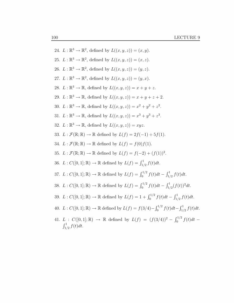
100 LECTURE 9
24. L : R3 → R
2, defined by L((x, y, z)) = (x, y).
25. L : R3 → R
2, defined by L((x, y, z)) = (x, z).
26. L : R3 → R
2, defined by L((x, y, z)) = (y, z).
27. L : R3 → R
2, defined by L((x, y, z)) = (y, x).
28. L : R3 → R, defined by L((x, y, z)) = x + y + z.
29. L : R3 → R, defined by L((x, y, z)) = x + y + z + 2.
30. L : R3 → R, defined by L((x, y, z)) = x2 + y2 + z2.
31. L : R3 → R, defined by L((x, y, z)) = x3 + y3 + z3.
32. L : R3 → R, defined by L((x, y, z)) = xyz.
33. L : F(R; R) → R defined by L(f) = 2f(−1) + 5f(1).
34. L : F(R; R) → R defined by L(f) = f(0)f(1).
35. L : F(R; R) → R defined by L(f) = f(−2) + (f(1))2.
36. L : C([0, 1]; R) → R defined by L(f) =∫ 1
1/2f(t)dt.
37. L : C([0, 1]; R) → R defined by L(f) =∫ 1/2
0f(t)dt −
∫ 1
1/2f(t)dt.
38. L : C([0, 1]; R) → R defined by L(f) =∫ 1/2
0f(t)dt −
∫ 1
1/2(f(t))2dt.
39. L : C([0, 1]; R) → R defined by L(f) = 1 +∫ 1/2
0f(t)dt −
∫ 1
1/2f(t)dt.
40. L : C([0, 1]; R) → R defined by L(f) = f(3/4)−∫ 1/2
0f(t)dt−
∫ 1
1/2f(t)dt.
41. L : C([0, 1]; R) → R defined by L(f) = (f(3/4))2 −∫ 1/2
0f(t)dt −∫ 1
1/2f(t)dt.

Lecture 10
Study Topics
• Real Matrices
• Linear Transformations Defined by Matrices
• Range and Kernel of a Matrix
101

102 LECTURE 10
In the previous lecture, we have studied a special class of functions from onereal vector space to another, namely those that were linear, and we calledthem linear functions, or, equivalently, linear mappings, or equivalently,linear transformations. In this lecture, we introduce the notion of a real“matrix”. What is a real matrix ? Think of it as a table, with, say m rowsand n columns, of real numbers. That’s it! So what’s the relation betweena matrix and a linear transformation ? As we will see in this lecture, areal matrix with m rows and n columns will allow us to define a lineartransformation from Rn to Rm.
Definition 12. Let m and n be integers ≥ 1. A real matrix with m rowsand n columns (also called a real m×n matrix) is a table (or array) of theform:
a1,1 a1,2 · · · a1,n
a2,1 a2,2 · · · a2,n...
... · · · ...am,1 am,2 · · · am,n
,
where all the entries (i.e. a1,1, a1,2, a1,3, · · · ) are real numbers.ai,j is called the entry of the matrix on row i and column j.
Let us look immediately at some examples:
1. The matrix
( √2
−π
)is a real 2 × 1 real matrix (2 rows, 1 column).
2. The matrix
(2 0
−1 1/√
3
)is a 2× 2 real matrix (2 rows, 2 columns).
3. The matrix
1 0−1 12 3
is a 3 × 2 real matrix (3 rows, 2 columns).
4. The matrix
(1 0 −2 1−1 1 2 3
)is a 2×4 real matrix (2 rows, 4 columns).
5. The matrix(
1 3 2 1 5)
is a 1×5 real matrix (1 row, 5 columns).
6. The matrix (−7) is a 1 × 1 real matrix (1 row, 1 column).

103
It is important to point out that the place of the elements in a matrix matters;exchanging the place of two elements in the matrix will change the matrix if
those two elements are not equal. For example, the matrices
(1 00 0
)and
(0 00 1
)are not equal. More generally, if A is defined to be the m×n real
matrix
A =
a1,1 a1,2 · · · a1,n
a2,1 a2,2 · · · a2,n...
... · · · ...am,1 am,2 · · · am,n
,
and B is defined to be the m × n real matrix
B =
b1,1 b1,2 · · · b1,n
b2,1 b2,2 · · · b2,n...
... · · · ...bm,1 bm,2 · · · bm,n
,
then we have A = B if and only if ai,j = bi,j for all 1 ≤ i ≤ m and all1 ≤ j ≤ n, i.e. the corresponding entries of A and B must be equal.
Definition 13. Let
A =
a1,1 a1,2 · · · a1,n
a2,1 a2,2 · · · a2,n...
... · · · ...am,1 am,2 · · · am,n
,
be a real m × n matrix. Let j ∈ {1, 2, · · · , n}. The jth column vector of A,
denoted by A;j is defined to be the element of Rm given by:
A;j =
a1,j
a2,j
a3,j...
am,j
.

104 LECTURE 10
Similarly, letting i ∈ {1, 2, · · · , m}, the ith row vector of A, denoted by Ai; isdefined to be the element of R
n given by:
Ai; = (ai,1, ai,2, ai,3, · · · , ai,n).
We shall very often write the row vector Ai; without the separating com-mas, i.e., as:
Ai; =(
ai,1 ai,2 ai,3 · · · ai,n
);
despite the lack of the separating commas, Ai; will still be understood as ann−tuple of real numbers, i.e. as an element of R
n.
Let us look at an example: Consider the 3 × 2 real matrix
3 2
−1 00 1
; its
first column vector is the element of R3 given by
3
−10
, and its second
column vector is the element of R3 given by
201
. Its first row vector is
the element of R2 given by (3, 2), its second row vector is the element of R
2
given by (−1, 0), and finally, its third row vector is the element of R2 given by
(0, 1). As was mentionned above, we shall often omit the separating commaswhen writing row vectors of matrices; for example, we shall write the firstrow vector of this matrix as
(3 2
)instead, and its second and third row
vectors as(−1 0
)and
(0 1
), respectively, and we shall still consider
them as elements of R2 (i.e. pairs of real numbers), despite the absence of
the separating commas.
Definition 14. Let m, n be integers ≥ 1. We denote the set of all m×n realmatrices by Mm,n(R).
In other words, an element of Mm,n(R) is nothing other than a real m × nmatrix, and any real m × n matrix is an element of Mm,n(R).
We now define two operations on Mm,n(R), namely addition of realmatrices and multiplication of a real matrix by a real number. Let
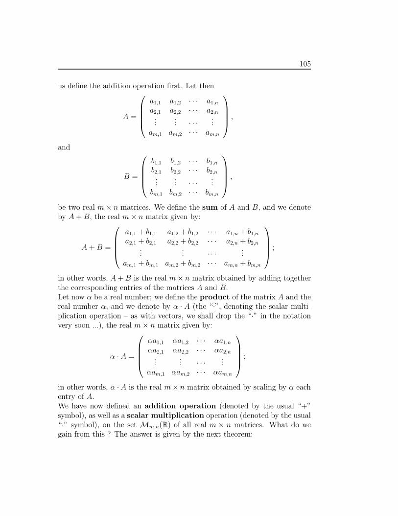
105
us define the addition operation first. Let then
A =
a1,1 a1,2 · · · a1,n
a2,1 a2,2 · · · a2,n...
... · · · ...am,1 am,2 · · · am,n
,
and
B =
b1,1 b1,2 · · · b1,n
b2,1 b2,2 · · · b2,n...
... · · · ...bm,1 bm,2 · · · bm,n
,
be two real m × n matrices. We define the sum of A and B, and we denoteby A + B, the real m × n matrix given by:
A + B =
a1,1 + b1,1 a1,2 + b1,2 · · · a1,n + b1,n
a2,1 + b2,1 a2,2 + b2,2 · · · a2,n + b2,n...
... · · · ...am,1 + bm,1 am,2 + bm,2 · · · am,n + bm,n
;
in other words, A + B is the real m× n matrix obtained by adding togetherthe corresponding entries of the matrices A and B.Let now α be a real number; we define the product of the matrix A and thereal number α, and we denote by α · A (the “·”, denoting the scalar multi-plication operation – as with vectors, we shall drop the “·” in the notationvery soon ...), the real m × n matrix given by:
α · A =
αa1,1 αa1,2 · · · αa1,n
αa2,1 αa2,2 · · · αa2,n...
... · · · ...αam,1 αam,2 · · · αam,n
;
in other words, α ·A is the real m× n matrix obtained by scaling by α eachentry of A.We have now defined an addition operation (denoted by the usual “+”symbol), as well as a scalar multiplication operation (denoted by the usual“·” symbol), on the set Mm,n(R) of all real m × n matrices. What do wegain from this ? The answer is given by the next theorem:
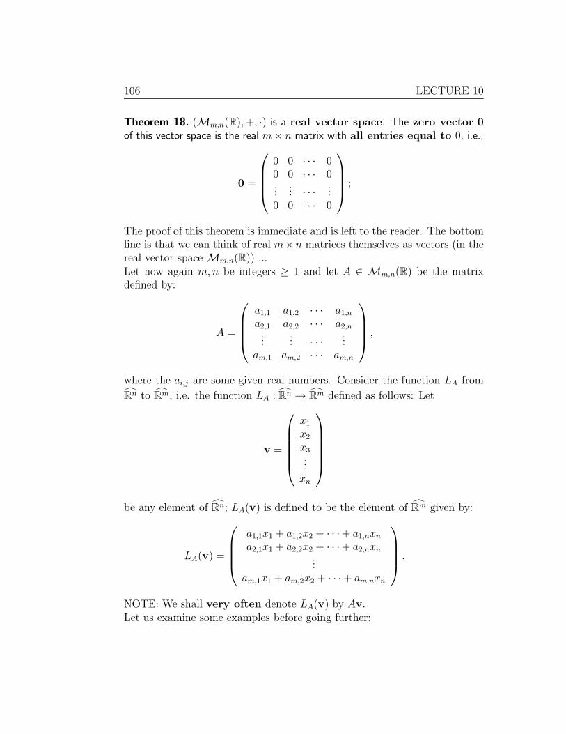
106 LECTURE 10
Theorem 18. (Mm,n(R), +, ·) is a real vector space. The zero vector 0of this vector space is the real m× n matrix with all entries equal to 0, i.e.,
0 =
0 0 · · · 00 0 · · · 0...
... · · · ...0 0 · · · 0
;
The proof of this theorem is immediate and is left to the reader. The bottomline is that we can think of real m×n matrices themselves as vectors (in thereal vector space Mm,n(R)) ...Let now again m, n be integers ≥ 1 and let A ∈ Mm,n(R) be the matrixdefined by:
A =
a1,1 a1,2 · · · a1,n
a2,1 a2,2 · · · a2,n...
... · · · ...am,1 am,2 · · · am,n
,
where the ai,j are some given real numbers. Consider the function LA from
Rn to Rm, i.e. the function LA : Rn → Rm defined as follows: Let
v =
x1
x2
x3...
xn
be any element of Rn; LA(v) is defined to be the element of Rm given by:
LA(v) =
a1,1x1 + a1,2x2 + · · ·+ a1,nxn
a2,1x1 + a2,2x2 + · · ·+ a2,nxn...
am,1x1 + am,2x2 + · · ·+ am,nxn
.
NOTE: We shall very often denote LA(v) by Av.Let us examine some examples before going further:
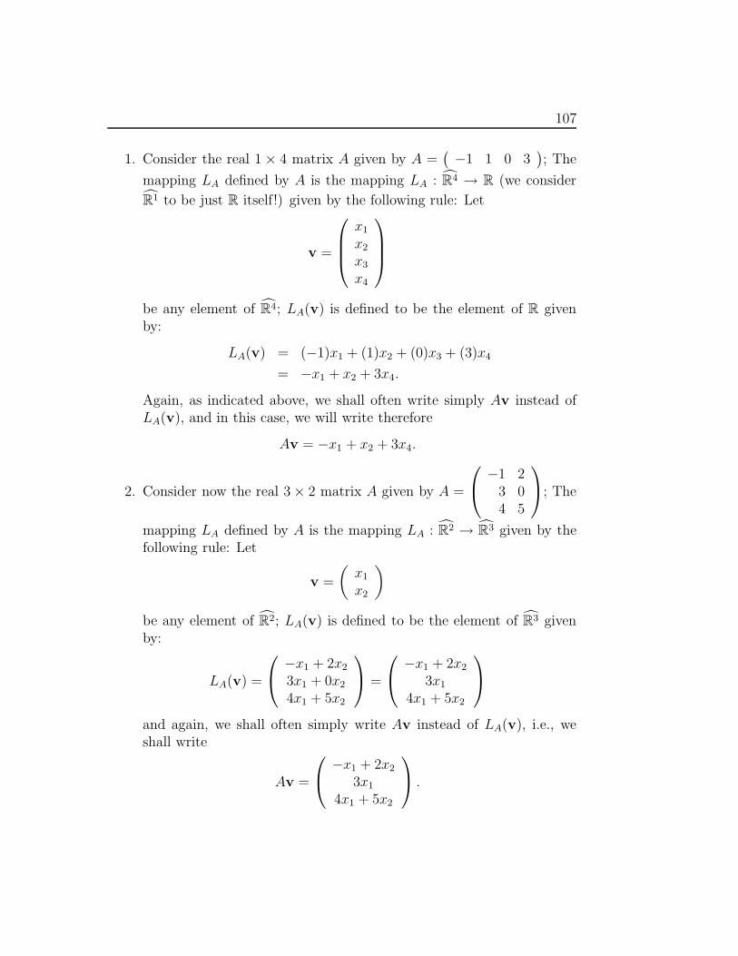
107
1. Consider the real 1 × 4 matrix A given by A =(−1 1 0 3
); The
mapping LA defined by A is the mapping LA : R4 → R (we consider
R1 to be just R itself!) given by the following rule: Let
v =
x1
x2
x3
x4
be any element of R4; LA(v) is defined to be the element of R givenby:
LA(v) = (−1)x1 + (1)x2 + (0)x3 + (3)x4
= −x1 + x2 + 3x4.
Again, as indicated above, we shall often write simply Av instead ofLA(v), and in this case, we will write therefore
Av = −x1 + x2 + 3x4.
2. Consider now the real 3 × 2 matrix A given by A =
−1 2
3 04 5
; The
mapping LA defined by A is the mapping LA : R2 → R3 given by thefollowing rule: Let
v =
(x1
x2
)
be any element of R2; LA(v) is defined to be the element of R3 givenby:
LA(v) =
−x1 + 2x2
3x1 + 0x2
4x1 + 5x2
=
−x1 + 2x2
3x1
4x1 + 5x2
and again, we shall often simply write Av instead of LA(v), i.e., weshall write
Av =
−x1 + 2x2
3x1
4x1 + 5x2
.
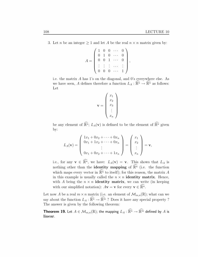
108 LECTURE 10
3. Let n be an integer ≥ 1 and let A be the real n × n matrix given by:
A =
1 0 0 · · · 00 1 0 · · · 00 0 1 · · · 0...
...... · · · ...
0 0 0 · · · 1
,
i.e. the matrix A has 1’s on the diagonal, and 0’s everywhere else. Aswe have seen, A defines therefore a function LA : Rn → Rn as follows:Let
v =
x1
x2
x3...
xn
be any element of Rn; LA(v) is defined to be the element of Rn givenby:
LA(v) =
1x1 + 0x2 + · · · + 0xn
0x1 + 1x2 + · · · + 0xn...
0x1 + 0x2 + · · · + 1xn
=
x1
x2...
xn
= v,
i.e., for any v ∈ Rn, we have: LA(v) = v. This shows that LA is
nothing other than the identity mapping of Rn (i.e. the function
which maps every vector in Rn to itself); for this reason, the matrix Ain this example is usually called the n × n identity matrix. Hence,with A being the n × n identity matrix, we can write (in keeping
with our simplified notation): Av = v for every v ∈ Rn.
Let now A be a real m×n matrix (i.e. an element of Mm,n(R); what can we
say about the function LA : Rn → Rm ? Does it have any special property ?The answer is given by the following theorem:
Theorem 19. Let A ∈ Mm,n(R); the mapping LA : Rn → Rm defined by A islinear.
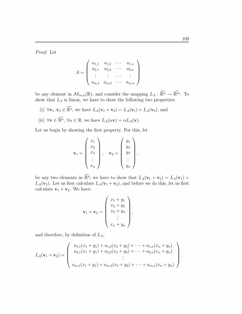
109
Proof. Let
A =
a1,1 a1,2 · · · a1,n
a2,1 a2,2 · · · a2,n...
... · · · ...am,1 am,2 · · · am,n
be any element in Mm,n(R), and consider the mapping LA : Rn → Rm. Toshow that LA is linear, we have to show the following two properties:
(i) ∀v1,v2 ∈ Rn, we have LA(v1 + v2) = LA(v1) + LA(v2), and
(ii) ∀v ∈ Rn, ∀α ∈ R, we have LA(αv) = αLA(v).
Let us begin by showing the first property. For this, let
v1 =
x1
x2
x3...
xn
, v2 =
y1
y2
y3...yn
,
be any two elements in Rn; we have to show that LA(v1 + v2) = LA(v1) +LA(v2). Let us first calculate LA(v1 + v2), and before we do this, let us firstcalculate v1 + v2. We have:
v1 + v2 =
x1 + y1
x2 + y2
x3 + y3...
xn + yn
,
and therefore, by definition of LA,
LA(v1 + v2) =
a1,1(x1 + y1) + a1,2(x2 + y2) + · · · + a1,n(xn + yn)a2,1(x1 + y1) + a2,2(x2 + y2) + · · · + a2,n(xn + yn)
...am,1(x1 + y1) + am,2(x2 + y2) + · · ·+ am,n(xn + yn)
.
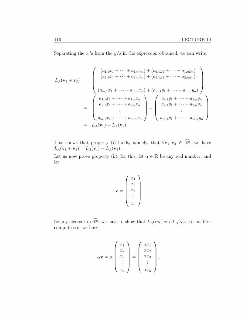
110 LECTURE 10
Separating the xi’s from the yj’s in the expression obtained, we can write:
LA(v1 + v2) =
(a1,1x1 + · · ·+ a1,nxn) + (a1,1y1 + · · · + a1,nyn)(a2,1x1 + · · ·+ a2,nxn) + (a2,1y1 + · · · + a2,nyn)
...(am,1x1 + · · ·+ am,nxn) + (am,1y1 + · · · + am,nyn)
=
a1,1x1 + · · ·+ a1,nxn
a2,1x1 + · · ·+ a2,nxn...
am,1x1 + · · ·+ am,nxn
+
a1,1y1 + · · ·+ a1,nyn
a2,1y1 + · · ·+ a2,nyn...
am,1y1 + · · ·+ am,nyn
= LA(v1) + LA(v2).
This shows that property (i) holds, namely, that ∀v1,v2 ∈ Rn, we haveLA(v1 + v2) = LA(v1) + LA(v2).
Let us now prove property (ii); for this, let α ∈ R be any real number, andlet
v =
x1
x2
x3...
xn
be any element in Rn; we have to show that LA(αv) = αLA(v). Let us firstcompute αv; we have:
αv = α
x1
x2
x3...
xn
=
αx1
αx2
αx3...
αxn
,

111
and therefore,
LA(αv) =
a1,1(αx1) + a1,2(αx2) + · · ·+ a1,n(αxn)a2,1(αx1) + a2,2(αx2) + · · ·+ a2,n(αxn)
...am,1(αx1) + am,2(αx2) + · · ·+ am,n(αxn)
=
α(a1,1x1 + a1,2x2 + · · · + a1,nxn)α(a2,1x1 + a2,2x2 + · · · + a2,nxn)
...α(am,1x1 + am,2x2 + · · ·+ am,nxn)
= α
a1,1x1 + a1,2x2 + · · ·+ a1,nxn
a2,1x1 + a2,2x2 + · · ·+ a2,nxn...
am,1x1 + am,2x2 + · · ·+ am,nxn
= αLA(v).
This proves property (ii), namely that ∀v ∈ Rn and ∀α ∈ R, we haveLA(αv) = αLA(v).Hence, LA satisfies properties (i) and (ii) and is therefore a linear mapping.
Now that we have shown that for any real m × n matrix A the mappingLA : Rn → Rm is linear, we can ask some further questions; in particular,we can try (in the spirit of the previous lecture) to identify the kernel andrange of LA ...Before we go any further, a few words on notation and terminology:
• As has been stated a number of times already, we shall often write Avinstead of LA(v); in that notation, the linearity of LA that we have justestablished means that A(v1 + v2) = Av1 + Av2 and A(αv) = αAv.
• We shall denote the kernel of LA by ker(A) instead of the more cum-bersome (but correct!) notation ker(LA), and we shall often just say“kernel of the matrix A” instead of the more cumbersome “kernelof the linear mapping LA defined by the matrix A”.
• Similarly, we shall denote the range of LA by Im(A) instead of themore cumbersome (but correct!) notation Im(LA), and we shall often

112 LECTURE 10
just say “range (or image) of the matrix A” instead of the morecumbersome “range (or image) of the linear mapping LA defined by thematrix A”.
Let then
A =
a1,1 a1,2 · · · a1,n
a2,1 a2,2 · · · a2,n...
... · · · ...am,1 am,2 · · · am,n
,
be a real m × n matrix (i.e. an element of Mm,n(R)), and let us first tryto identify the range of A, i.e. the range of the linear mapping LA :Rn → Rm. Recall that the range of LA, which we shall simply write asIm(A), is the set of all LA(v) in Rm with v in Rn; i.e., writing this formally,we have:
Im(A) = {LA(v)|v ∈ Rn}.
Let now
v =
x1
x2
x3...
xn
be any element in Rn; we can write:
LA(v) =
a1,1x1 + a1,2x2 + · · ·+ a1,nxn
a2,1x1 + a2,2x2 + · · ·+ a2,nxn...
am,1x1 + am,2x2 + · · · + am,nxn
= x1
a1,1
a2,1...
am,1
+ x2
a1,2
a2,2...
am,2
+ · · · + xn
a1,n
a2,n...
am,n
= x1A;1 + x2A;2 + · · ·xnA;n,
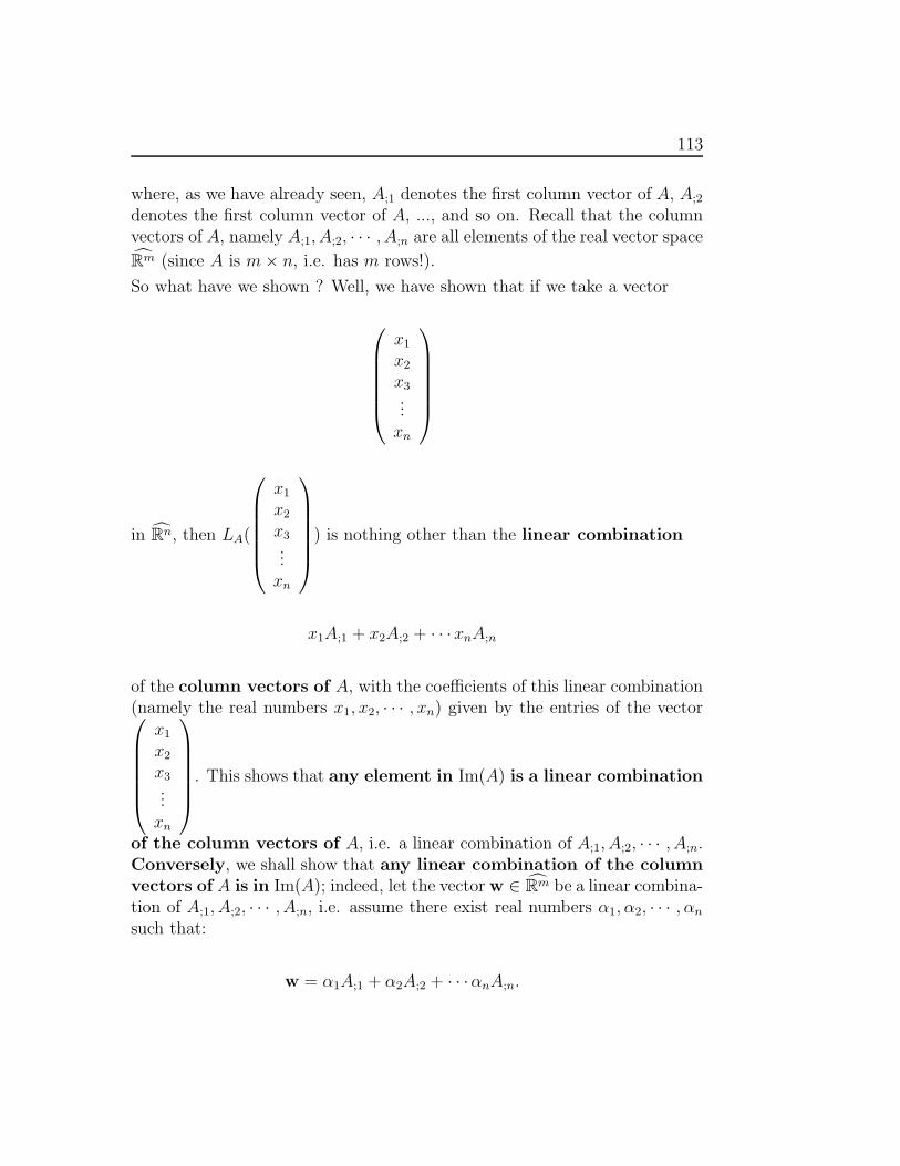
113
where, as we have already seen, A;1 denotes the first column vector of A, A;2
denotes the first column vector of A, ..., and so on. Recall that the columnvectors of A, namely A;1, A;2, · · · , A;n are all elements of the real vector space
Rm (since A is m × n, i.e. has m rows!).
So what have we shown ? Well, we have shown that if we take a vector
x1
x2
x3...
xn
in Rn, then LA(
x1
x2
x3...
xn
) is nothing other than the linear combination
x1A;1 + x2A;2 + · · ·xnA;n
of the column vectors of A, with the coefficients of this linear combination(namely the real numbers x1, x2, · · · , xn) given by the entries of the vector
x1
x2
x3...
xn
. This shows that any element in Im(A) is a linear combination
of the column vectors of A, i.e. a linear combination of A;1, A;2, · · · , A;n.Conversely, we shall show that any linear combination of the columnvectors of A is in Im(A); indeed, let the vector w ∈ Rm be a linear combina-tion of A;1, A;2, · · · , A;n, i.e. assume there exist real numbers α1, α2, · · · , αn
such that:
w = α1A;1 + α2A;2 + · · ·αnA;n.

114 LECTURE 10
We therefore have:
w = α1
a1,1
a2,1...
am,1
+ α2
a1,2
a2,2...
am,2
+ · · ·+ αn
a1,n
a2,n...
am,n
=
a1,1α1 + a1,2α2 + · · · + a1,nαn
a2,1α1 + a2,2α2 + · · · + a2,nαn...
am,1α1 + am,2α2 + · · ·+ am,nαn
= LA(
α1
α2
α3...
αn
),
which shows that w is in Im(A) (since it is LA of something in Rn!).Let us recapitulate what we have shown: We have shown that if A is a realm × n matrix, then Im(A) (i.e. the range of the linear mapping LA : Rn →Rm) is the set of all linear combinations of the column vectors ofA; but we already have a name for this! The set of all linear combinationsof the column vectors of A is nothing other than the vector subspace of Rm
generated by the column vectors of A, i.e. the linear span of the columnvectors of A. We have therefore proved the following theorem:
Theorem 20. Let A be a real m×n matrix; the range Im(A) of the matrix
A (i.e. the range of the linear mapping LA : Rn → Rm) is the linear span ofthe column vectors A;1, A;2, · · · , A;n of A.
Let us consider some examples:
1. Let A be the real 2×3 matrix given by A =
(1 0 12 3 5
); then, Im(A) is
the vector subspace of R2 generated by the subset {(
12
),
(03
),
(15
)}
of R2; in other words, Im(A) is the linear span of {(
12
),
(03
),
(15
)}.
115
It is easy to show that the linear span of this set is R2 itself (for ex-
ample, one can easily show that any vector in R2 can be written as a
linear combination of the first two vectors, i.e.
(12
)and
(03
)), and
hence Im(A) = R2.
2. Let now A be the real 4 × 2 matrix given by A =
−1 00 1
−2 31 −3
;
then, Im(A) is the vector subspace of R4 generated by the sub-
set {
−10
−21
,
013
−3
} of R4; in other words, Im(A) is the linear
span of {
−10
−21
,
013
−3
}. Could it be the case here that Im(A)
is R4 itself ? Well, we know from Lecture 8 that R4 has dimen-sion 4; we also know from Theorem 10 of Lecture 8 that if a subsetS of an N−dimensional real vector space V is a generating set forV, then the number of elements of S must be ≥ N . In our case,
S = {
−10
−21
,
013
−3
}, and therefore has only 2 elements (and 2 is
not ≥ 4); we conclude that Im(A) 6= R4.
The observations made in these two examples can be packaged into a theorem:
Theorem 21. Let A be a real m× n matrix (i.e. with m rows and n columns).We have:
• If Im(A) = Rm, then we must have n ≥ m. Hence, if n < m, then Im(A)
cannot be equal to Rm.
Proof. We know that Im(A) is equal to the linear span of the n column vectors
A;1, A;2, · · · , A;n of A. Recall that each of A;1, A;2, · · · , A;n is a vector in Rm.
116 LECTURE 10
If Im(A) = Rm, then the subset {A;1, A;2, · · · , A;n} is a generating set for
Rm; that generating subset has n elements and Rm has dimension m (wehave seen this in Lecture 8), and it follows therefore from Theorem 10 of
Lecture 8 that if Im(A) = Rm then we must have n ≥ m.
Now that we have investigated the range Im(A) of a real matrix A, let usexamine its kernel ker(A) (again, by ker(A) we mean the kernel of the linearmap LA defined by A, i.e. ker(LA)). Let then
A =
a1,1 a1,2 · · · a1,n
a2,1 a2,2 · · · a2,n...
... · · · ...am,1 am,2 · · · am,n
,
be a real m × n matrix, and let us try to get some information about thekernel ker(A) of A. By definition of ker(A), a vector v of Rn is in ker(A) if
and only if LA(v) = 0dRm (where 0dRm =
0...0
denotes the zero vector of
Rm); let us be more precise. Let then
v =
x1
x2
x3...
xn
be any element in Rn; We have seen already that
LA(v) = x1A;1 + x2A;2 + · · ·xnA;n,
where A;1, A;2, · · · , A;n are the column vectors of A.
Assume now that A;1, A;2, · · · , A;n are linearly independent. Then, theequality
LA(v) = 0dRm

117
(where 0dRm =
0...0
denotes the zero vector of Rm) is equivalent to the
equality
x1A;1 + x2A;2 + · · ·xnA;n = 0dRm ,
which, by linear independence of A;1, A;2, · · · , A;n, implies x1 = x2 = · · · =
xn = 0, i.e. v = 0cRn , i.e. v is the zero vector of Rn. In other words, we haveshown that if the column vectors of A are linearly independent, then thekernel of LA (which we denote by ker(A)) is just {0cRn}, i.e. ker(A) = {0cRn}.Let us now prove the converse. Assume therefore that ker(A) = {0cRn}; wewould like to show that the column vectors of A are then linearly independent.Let then α1, α2, · · · , αn be real numbers such that
α1A;1 + α2A;2 + · · ·+ αnA;n = 0dRm ;
we want to show that α1, α2, · · · , αn must then all be zero. Now let v ∈ Rn
be given by:
v =
α1
α2
α3...
αn
.
The equality
α1A;1 + α2A;2 + · · ·+ αnA;n = 0dRm ;
can be written
LA(v) = 0dRm
which implies v ∈ ker(A) (by definition of ker(A)), and since we have as-sumed that ker(A) = {0cRn}, it follows that v = 0cRn, i.e.
α1
α2
α3...
αn
=
000...0
,

118 LECTURE 10
which implies α1 = α2 = · · · = αn = 0, as desired. This proves that thecolumn vectors A;1, A;2, · · · , A;n of A are linearly independent.In summary, we have proved the following theorem:
Theorem 22. Let A ∈ Mm,n(R) (i.e. A is a real m × n matrix). We haveker(A) = {0cRn} if and only if the column vectors of A are linearly inde-pendent.
We close this section with some important terminology and an importanttheorem which is a direct adaptation of the Rank-Nullity Theorem ofLecture 9:
Definition 15. Let A ∈ Mm,n(R), i.e. A is a real m × n matrix.
(i) The rank of A is defined to be the dimension of Im(A), and is denotedby rank(A).
(ii) The nullity of A is defined to be the dimension of ker(A), and isdenoted by nullity(A).
Theorem 23. Let A ∈ Mm,n(R); then:
rank(A) + nullity(A) = n,
i.e. rank(A) + nullity(A) is equal to the number of columns of A.
Proof. The result follows directly from the Rank-Nullity Theorem of Lec-ture 9, taking into account the fact that:
• rank(A) is by definition the dimension of Im(LA) (which we havedenoted Im(A)),
• nullity(A) is by definition the dimension of ker(LA) (which we havedenoted ker(A)),
• LA is a linear mapping from the real vector space Rn to the realvector space Rm,
• Rn is a real vector space of dimension n.
119
PROBLEMS:
1. For each of the following choices for the matrix A, do the following:
• Specify the linear transformation LA that it defines (for example,
if A =
(1 02 1
), then LA is the mapping LA : R2 → R2 defined
by LA(
(x1
x2
)) =
(x1
2x1 + x2
), for every
(x1
x2
)∈ R2,
• specify its range Im(A) as well as the dimension of Im(A),
• specify its kernel ker(A) as well as the dimension of ker(A);
• verify the Rank-Nullity theorem for A (i.e. verify that dim(Im(A))+dim(ker(A)) = number of columns of A).
(a) A =(−1 2
).
(b) A =
(−12
).
(c) A =(
1 0 3).
(d) A =
(3 2 10 0 0
).
(e) A =
(0 00 0
).
(f) A =
(1 00 1
).
(g) A =
(1 0 00 1 0
).
(h) A =
1 0 00 1 00 0 1
.
(i) A =
1 22 1
−1 3
.

120 LECTURE 10
(j) A =
1 01 −10 01 0
.
(k) A =
1 0 01 −1 10 0 21 0 −1
.
(l) A =
2 0 00 2 00 0 2
.
(m) A =
(5 0 0 00 5 0 0
).
(n) A =
(0 5 0 00 0 5 0
).
(o) A =
(0 0 5 00 0 0 5
).
(p) A =
5 0 0 00 5 0 00 0 5 00 0 0 5
.
(q) A =
(3 0 0 00 −2 0 0
).
(r) A =
(0 3 0 00 0 −1 0
).
(s) A =
(0 0 3 10 0 −1 0
).

Lecture 11
Study Topics
• Systems of Linear Transformations Revisited
• Solving Systems of Linear Equations
121
122 LECTURE 11
Consider the system of linear equations in m equations and n unknowns givenby:
(E)
a1,1x1 + a1,2x2 + a1,3x3 + · · ·a1,nxn = b1
a2,1x1 + a2,2x2 + a2,3x3 + · · ·a2,nxn = b2
a3,1x1 + a3,2x2 + a3,3x3 + · · ·a3,nxn = b3
am,1x1 + am,2x2 + am,3x3 + · · ·am,nxn = bm
where the real numbers a1,1, a1,2, · · · , am,n and b1, b2, · · · , bm are given realnumbers, and we wish to solve for the real numbers x1, x2, · · · , xn.Can we write this system in terms of matrices and vectors ? Before answeringthis question, you may ask what the point of writing such a system in termsof matrices and vectors would be. The answer to this last question is quitesimple: If we are able to write that system of equations in terms of matricesand vectors, then with the linear algebra knowledge we have accumulatedso far, we may be able to say something interesting about that system ofequations: For example, whether or not it has a solution, how many solutionsit does have, and so on, and even beyond this, in case it does have a solution,how to go about finding that solution. So let us not waste any time and letus try to express that system of linear equations using matrices and vectors.Let then A ∈ Mm,n(R) be the real m × n matrix defined by
A =
a1,1 a1,2 · · · a1,n
a2,1 a2,2 · · · a2,n...
... · · · ...a1,1 a1,2 · · · a1,n
,
and let b ∈ Rm be the real vector defined by
b =
b1
b2...
bm
.
It is easy to verify that the real numbers x1, x2, · · · , xn satisfy the abovesystem of linear equations if and only if the vector v ∈ Rn defined by
v =
x1
x2...
xn
.

123
satisfies the vector equation (so called because the unknown is now a vector
in Rn):
LA(v) = b.
Note that in keeping with our simplified notation (i.e. writing Av instead ofLA(v)), we can write this last equation simply as
Av = b.
Before going further, let us now see how easily we can prove that our originalsystem of linear equations (E) can have only 0, 1 or infinitely many solutions.We already proved this in Lecture 6, but let us prove it again here.From the discussion above, we need only show therefore that the equationLA(v) = b, where A ∈ Mm,n(R) and b ∈ Rm are given, and where we wish
to solve for the unknown vector v ∈ Rn, can have only 0, 1 or infinitely manysolutions. We have the following cases:
(Case 1) b /∈ Im(A). In this case, there is no v ∈ Rn which satisfies LA(v) = b(since otherwise b would be in Im(A)), i.e. there is no solution.
(Case 2) b ∈ Im(A). In this case, there is at least one vector in Rn which satisfiesthe equation LA(v) = b; let v1 be one such vector (i.e. LA(v1) = b).To find out how many other vectors satisfy that equation, we considerthe following two subcases:
(Case 2a) ker(A) = {0cRn}. In this subcase LA is one-to-one and hence
there is a unique v ∈ Rn which satisfies LA(v) = b, namely v1.
(Case 2b) ker(A) 6= {0cRn}. In this subcase, there is a non-zero vector
w ∈ ker(A), i.e w 6= 0cRn . Since ker(A) is a vector subspace of Rn,we have αw ∈ ker(A), ∀α ∈ R. Then, ∀α ∈ R:
LA(v1 + αw) = LA(v1) + LA(αw) = b + αLA(w) = b + 0dRm = b,
which shows that v1+αw is also a solution to the vector equationLA(v) = b. There are infinitely many distinct vectors of the formv1 + αw (one for each choice of the real number α), and hence inthis subcase, there are infinitely many solutions to the vectorequation LA(v) = b.
124 LECTURE 11
And this completes the proof!There are two important points to take away from this:
1. The ease with which that non-trivial result is proved,
2. The key role played by the range Im(A) and the kernel ker(A) indetermining the number of solutions to the equation LA(v) = b.
Now that we have seen that a system of linear equations can be writtenvery compactly using matrices and vectors in the form of a vector equationLA(v) = b (with A,b given, and v the unknown), let us try to use thisconnection to further our understanding of systems of linear equations. Inparticular, let us examine the following question:
• Let A ∈ Mm,n(R); under what conditions on A does there exist, for
each choice of b ∈ Rm, a unique solution to the equation LA(v) = b?
The answer to this important question is given in the next theorem:
Theorem 24. Let A ∈ Mm,n(R). We have the following:
(a) If, for each b ∈ Rm, there exists a unique v ∈ Rn which satisfiesLA(v) = b, then m = n and the column vectors of A are linearlyindependent.
(b) Conversely, if m = n and the column vectors of A are linearly inde-
pendent, then for each b ∈ Rm, there exists a unique v ∈ Rn whichsatisfies LA(v) = b.
Proof. (a) Assume that for each b ∈ Rm there exists a unique v ∈ Rn which
satisfies LA(v) = b; since for each b ∈ Rm the equation LA(v) = b
has a solution, it follows that Im(A) = Rm, which implies that m ≤ n;furthermore, since that solution is unique, it follows that ker(A) ={0cRn}, which implies that m ≥ n. Since we have both m ≤ n andm ≥ n, it follows that m = n.
(b) Assume now that m = n and that the column vectors of A are linearlyindependent. Since the n column vectors A;1, A;2, · · · , A;n of A are
elements of Rn (since m = n), since they are assumed to be linearly
125
independent, and since Rn has dimension n, it follows (from Lecture
8) that {A;1, A;2, · · · , A;n} is also a generating set for Rn, i.e. that
Im(A) = Rn. Hence, for each b ∈ Rm, there is at least one vector
v ∈ Rn which satisfies LA(v) = b. Furthermore, since the columnvectors of A are assumed to be linearly independent, it follows (fromLecture 10) that ker(A) = {0cRn}, and therefore (again from lecture 10),
for each b ∈ Rm, there is a unique v ∈ Rn which satisfies LA(v) = b.
Now that, thanks to this last theorem, we have the answer to the questionwe posed earlier, let us examine how we could go about solving an equationof the form LA(v) = b, with A a square n × n real matrix.
NOTE: For simplicity, we will denote the set of all square n×n real matricessimply by Mn(R).
Let then A ∈ Mn(R), and let b ∈ Rn. We wish to find v ∈ Rn which satisfies
LA(v) = b.
Assume that there exist some matrix B ∈ Mn(R) such that LB(LA(v)) = v
for all v ∈ Rn, i.e., such that LB ◦ LA(v) = v for all v ∈ Rn; how can theknowledge of this matrix B help us solve our equation ? Well, if some vectorof Rn, say w, satisfies the equation
LA(w) = b,
then, applying LB to both sides, it must also satisfy the equation
LB(LA(w)) = LB(b),
and since we assumed B was such that LB(LA(v)) = v for all v ∈ Rn, itfollows that w must also satisfy
w = LB(b),
i.e. w must be equal to LB(b), i.e. the solution to the equation LA(v) = bis given by v = LB(b); in other words, we have solved the equation!Let us examine this idea on an example before going further:
126 LECTURE 11
• Let A ∈ M2(R) be the square 2 × 2 matrix defined by A =
(4 13 1
),
and let b ∈ R2 be the vector defined by b =
(b1
b2
). We wish to find
v ∈ R2 such that LA(v) = b. Note that since the column vectors of Aare linearly independent (as can be easily verified), it follows that for
any b ∈ R2, the equation LA(v) = b has a unique solution. Let now
B ∈ M2(R) be the square 2 × 2 matrix defined by B =
(1 −1
−3 4
).
Let now v =
(x1
x2
)be any vector in R2. We have:
LB ◦ LA(v) = LB(LA(v))
= LB(
(4x1 + x2
3x1 + x2
))
=
((4x1 + x2) − (3x1 + x2)
−3(4x1 + x2) + 4(3x1 + x2)
)
=
(x1
x2
)
= v,
We have shown therefore that ∀v ∈ R2, LB ◦ LA(v) = v. Thanks tothis, and in line with our previous discussion, we can solve the vector
equation LA(v) = b; indeed, let v ∈ R2 satisfy LA(v) = b. Then,applying LB to both sides yields the equality:
LB ◦ LA(v) = LB(b),
i.e., equivalently,
v = LB(b) = LB(
(b1
b2
)) =
(b1 − b2
−3b1 + 4b2
).
Hence, thanks to the fact that we got our hands on that special matrixB, we were able to solve our vector equation.
The natural questions one may ask at this point are:
• How did this matrix B show up ?
• How does one find such a matrix B in a systematic way ?
We will have the complete answer to these questions in the next few lectures.
Lecture 12
Study Topics
• Matrix Multiplication
127

128 LECTURE 12
Let m, n, p be given integers ≥ 1, let A ∈ Mm,n(R) be the real m×n matrixdefined by
A =
a1,1 · · · a1,n... · · · ...
am,1 · · · am,n
,
and let B ∈ Mn,p(R) be the real n × p matrix defined by
B =
b1,1 · · · b1,p... · · · ...
bn,1 · · · bn,p
.
Before going further, let us pay attention to the fact that A has m rowsand n columns whereas B has n rows and p columns; in particular thenumber of columns of A is equal to the number of rows of B.We know that A defines the linear mapping
LA : Rn → Rm,
and similarly, B defines the linear mapping
LB : Rp → Rn.
Note that since LA maps from Rn and since LB maps to Rn, we can composethese two mappings and obtain the mapping LA ◦ LB : Rp → Rm, which isdefined by:
LA ◦ LB(v) = LA(LB(v)), ∀v ∈ Rp.
What do we know about LA ◦ LB ? Well, it is the composition of twolinear mappings (namely LA and LB) hence it is also linear. But thereis more! We will soon see that LA ◦ LB is actually equal to LC where C isa real m × p matrix obtained from A and B ...Let us begin by computing LA ◦ LB(v). Let then v ∈ Rp be given by
v =
x1
x2...
xp
;

129
then, we obtain:
LB(v) =
b1,1x1 + · · · + b1,pxp...
bn,1x1 + · · · + bn,pxp
,
and hence
LA ◦ LB(v) =
a1,1(b1,1x1 + · · · + b1,pxp) + · · ·+ a1,n(bn,1x1 + · · ·+ bn,pxp)...
am,1(b1,1x1 + · · · + b1,pxp) + · · ·+ am,n(bn,1x1 + · · ·+ bn,pxp)
=
(a1,1b1,1 + · · ·+ a1,nbn,1)x1 + · · · + (a1,1b1,p + · · ·a1,nbn,p)xp...
(am,1b1,1 + · · · + am,nbn,1)x1 + · · · + (am,1b1,p + · · ·am,nbn,p)xp
= LC(v),
where C ∈ Mm,p(R) is the real m × p matrix given by
C =
c1,1 c1,2 · · · c1,p
c2,1 c2,2 · · · c2,p...
... · · · ...cm,1 cm,2 · · · cm,p
with ci,j given by
ci,j = ai,1b1,j + ai,2b2,j + ai,3b3,j + · · ·+ ai,nbn,j
=n∑
k=1
ai,kbk,j
for every 1 ≤ i ≤ m and 1 ≤ j ≤ p. We call C the product of A and Band we write C = AB. NOTE: C has the same number of rows as A, andthe same number of columns as B.Let us consider a few examples:
1. Let A be the 2 × 3 matrix given by A =
(1 2 03 5 1
), and let B be
the 2 × 2 matrix given by B =
(1 03 5
); we wish to compute the

130 LECTURE 12
product AB of A and B. But this is not possible, since the numberof columns of A is not equal to the number of rows of B. Hence, theproduct AB does not make any sense! On the other hand, the numberof columns of B is indeed equal to the number of rows of A, so it doesmake sense to compute the product BA, and we obtain the 2×3 realmatrix (with the “·” denoting ordinary multiplication):
BA =
(1 · 1 + 0 · 3 1 · 2 + 0 · 5 1 · 0 + 0 · 13 · 1 + 5 · 3 3 · 2 + 5 · 5 3 · 0 + 5 · 1
)
=
(1 2 018 31 5
)
2. Let A be the real m × n matrix given by
A =
a1,1 · · · a1,n... · · · ...
am,1 · · · am,n
,
and let v be the real n × 1 matrix (i.e. the column vector) given by:
v =
x1
x2...
xn
;
Since the number of columns of A (namely n) is equal to the numberof rows of v, it makes sense to consider the product Av of these twomatrices, and we obtain the m × 1 real matrix:
Av =
a1,1x1 + · · · + a1,nxn
a2,1x1 + · · · + a2,nxn...
am,1x1 + · · · + am,nxn
which is nothing other than LA(v) !!!! This is why we shall oftensimply write Av instead of LA(v) ...

131
3. Let now A ∈ Mn(R) be the real n × n (square) matrix given by
A =
1 0 0 · · · 00 1 0 · · · 00 0 1 · · · 0...
...... · · · ...
0 0 0 · · · 1
,
(i.e. 1’s on the diagonal, and 0’s everywhere else), and let B ∈ Mn,p(R)be a real n×p matrix. Since the number of columns of A (namely n) isequal to the number of rows of B, it makes sense to consider the matrixproduct AB. AB has n rows and p columns, just like B. Furthermore,a simple computation shows that AB = B for any B ∈ Mn,p(R). Forthis reason, (as we have seen before), this particular matrix A is calledthe n × n identity matrix.
4. Let now A ∈ M3,2(R) be the real 3 × 2 matrix given by
A =
1 10 2
−1 1
,
and B ∈ M2,3(R) be the real 2 × 3 matrix given by
B =
(1 3 02 1 1
);
since the number of columns of A (namely 2) is equal to the numberof rows of B, it makes sense to consider the matrix product AB, andwe obtain after a simple computation that AB is the 3× 3 real matrixgiven by:
AB =
3 4 14 2 21 −2 1
.
Note that since in this particular case the number of columns of B(namely 3) is equal to the number of rows of A, it also makes sense to
132 LECTURE 12
compute the matrix product BA, and we obtain after a simple compu-tation that BA is the 2 × 2 real matrix given by:
BA =
(1 71 5
).
Note that in this particular example where both AB and BA madesense, AB and BA ended up being of different types: AB is 3 × 3whereas BA is 2 × 2. The next example shows that even when ABand BA are of the same type, they are not necessarily equal ...
5. Let now A and B both be real 2×2 matrices (so both matrix productsAB and BA make sense in this case) given by:
A =
(0 10 0
), B =
(0 01 0
).
We obtain for AB:
AB =
(1 00 0
),
whereas
BA =
(0 00 1
),
which shows that AB is not equal to BA. So keep in mind thatmatrix multiplication is NOT like ordinary multiplication ofreal numbers! (Another way to put this is that matrix multiplicationis not commutative).
6. Let A ∈ Mm,n(R) be a real m × n matrix, and let B ∈ Mn,p(R) bea real n × p matrix. Denote the p column vectors of B by (in or-der) B;1, B;2, · · · , B;p, i.e. we can write B = (B;1 B;2 · · · B;p). Itis easy to verify that the matrix product AB has columns vectorsgiven (in order) by AB;1, AB;2, · · · , AB;p, i.e., we can write AB =(AB;1 AB;2 · · · AB;p). This is often useful in proofs ...
Now that we have seen the “mechanics” of matrix multiplication, let usexamine some of its properties:

133
Theorem 25. Matrix multiplication satisfies the following properties:
(i) Let m, n, p, q be integers ≥ 1. ∀A ∈ Mm,n(R), ∀B ∈ Mn,p(R), and∀C ∈ Mp,q(R), we have:
(AB)C = A(BC),
i.e. matrix multiplication is associative.
(ii) Let m, n, p be integers ≥ 1. ∀A ∈ Mm,n(R), ∀B, C ∈ Mn,p(R), we have:
A(B + C) = AB + AC
(iii) Let m, n, p be integers ≥ 1. ∀A, B ∈ Mm,n(R), ∀C ∈ Mn,p(R), we have:
(A + B)C = AC + BC
(iv) Let m, n, p be integers ≥ 1. ∀A ∈ Mm,n(R), ∀B ∈ Mn,p(R), ∀λ ∈ R,we have:
A(λB) = (λA)B = λ(AB).
NOTE: What statement (i) of the theorem says is that we can first multiplyA and B to obtain AB, and then multiply this with C to obtain (AB)C;we can also first multiply B and C to obtain BC and then multiply A withBC to obtain A(BC). Both give the same result. Hence, we can remove theparentheses and simply write ABC instead of either (AB)C or A(BC).
We shall only prove (i); Properties (ii),(iii),(iv) can be directly verified bycomputation and are left as an exercise to the reader.
Proof. Recall that the matrix product AB is defined by LAB = LA ◦LB ; sim-ilarly, the matrix product (AB)C is defined by L(AB)C = LAB ◦ LC . Hence,L(AB)C = (LA ◦LB) ◦LC , and since composition of functions is associa-tive, we have
L(AB)C = (LA ◦ LB) ◦ LC = LA ◦ (LB ◦ LC) = LA ◦ LBC = LA(BC),
which implies (AB)C = A(BC), and this proves (i).

134 LECTURE 12
Let us now see on some simple examples how we can apply matrix op-erations to the solution of systems of linear equations:
1. Consider the system of linear equations given by
2x + 3y = 5
3x + y = 7,
where we wish to solve for the pair (x, y) of real numbers which satisfiesthat system, if such a pair does exist. We can write this equation inmatrix form as:
(2 33 1
) (xy
)=
(57
),
and since the column vectors of the 2×2 matrix
(2 33 1
)are linearly
independent we know that this system has a unique solution. Con-
sider now the 2 × 2 matrix given by
(−1
737
37
−27
). It is easy to verify
that(
−17
37
37
−27
) (2 33 1
)=
(1 00 1
),
which is nothing other than the 2 × 2 identity matrix. Hence, multi-plying both sides of the equation
(2 33 1
) (xy
)=
(57
),
by the matrix
(−1
737
37
−27
), we obtain
(−1
737
37
−27
) (2 33 1
) (xy
)=
(−1
737
37
−27
) (57
),
i.e., equivalently,
(1 00 1
) (xy
)=
(16717
),

135
and since(
1 00 1
) (xy
)=
(xy
),
we finally obtain the solution to our system of equations as(
xy
)=
(16717
).
2. More generally, consider the system of linear equations (in n equationsand n unknowns) given by
a1,1x1 + · · ·a1,nxn = b1
a2,1x1 + · · ·a2,nxn = b2
an,1x1 + · · ·an,nxn = b1
where we wish to solve for the n−tuples (x1, x2, · · · , xn) of real num-bers. We can write this system in matrix form as:
Av = b,
where A ∈ Mn(R) is the square n × n matrix given by
A =
a1,1 a1,2 · · · a1,n
a2,1 a2,2 · · · a2,n...
... · · · ...a1,1 a1,2 · · · a1,n
,
b ∈ Mn,1(R) is the n × 1 matrix (i.e. column vector) given by
b =
b1
b2...bn
,
and, finally,
v =
x1
x2...
xn
,
136 LECTURE 12
is the n× 1 matrix (i.e. column vector) we wish to solve for. Assumethere exists a matrix B ∈ Mn(R) such that the matrix product ofB and A, i.e. BA, is equal to the n × n identity matrix. Then,multiplying (to the left) both sides of the equality
Av = b,
by B yields
BAv = Bb,
and since BA is the n × n identity matrix, we obtain
v = Bb,
i.e. we have the solution to our original system of equations. In thenext lectures, we will see when such a matrix B does exist and howto compute it.
PROBLEMS:
1. For each of the following choices for the matrices A and B, do thefollowing:
• Specify whether it makes sense to consider the matrix productAB (and indicate why or why not), and if the product AB makessense, do compute it.
• Specify whether it makes sense to consider the matrix productBA (and indicate why or why not), and if the product BA makessense, do compute it.
(a) A =(−1 2
), B =
(1 20 −1
).
(b) A =(−1 2
), B =
(1 00 1
).
(c) A =(−1 2
), B =
(0 11 0
).

137
(d) A =(−1 2
), B =
(0 1
).
(e) A =(−1 2
), B =
0 11 02 2
.
(g) A =
(−1 23 5
), B =
(1 −35 1
).
(h) A =
(0 10 0
), B =
(2 −30 0
).
(i) A =
(−1 23 5
), B =
(1 00 1
).
(j) A =
(−1 23 5
), B =
(0 11 0
).
(k) A =
−1 23 57 4
, B =
(1 10 1
).
(l) A =
−1 23 57 4
, B =
(1 00 1
).
(m) A =
−1 23 57 4
, B =
(0 11 0
).
(n) A =
−1 23 57 4
, B =
1 2 20 1 −3
−2 0 1
.
(o) A =
−1 23 57 4
, B =
1 0 00 2 00 0 −1
.
(p) A =
−1 23 57 4
, B =
0 1 01 5 70 0 1
.
(q) A =
−1 2 5
3 −2 57 0 4
, B =
1 0 00 1 00 0 1
.

138 LECTURE 12
(r) A =
−1 2 5
3 −2 57 0 4
, B =
1 0 00 0 10 1 0
.
(s) A =
−1 2 5
3 −2 57 0 4
, B =
0 0 10 1 01 0 0
.
(t) A =
−1 2 5
3 −2 57 0 4
, B =
0 1 01 0 00 0 1
.
(u) A =
−2 1
1 23 0
, B =
(1 2 10 3 5
).
(v) A =
−2 1
1 03 2
, B =
1 0 00 1 00 0 1
.
(w) A =
−1 3
0 01 5
, B =
0 1 01 0 00 0 1
.
(x) A =
−3 3
2 7−2 −5
, B =
(11
).
(y) A =
−1 23 57 4
, B =
121
.
(z) A =
−5 −2−3 1−2 0
, B =
1 0 1 01 2 0 00 3 0 1
.
Lecture 13
Study Topics
• Invertible Square Matrices
• Determinant of a Square Matrix
139
140 LECTURE 13
Let A ∈ Mn(R) be the square n × n real matrix given by
A =
a1,1 a1,2 · · · a1,n
a2,1 a2,2 · · · a2,n...
... · · · · · ·an,1 an,2 · · · an,n
.
We have already seen in the previous lectures what use we could make of theexistence of a real n×n matrix B such that the matrix product BA be equalto the n × n identity matrix. Indeed (let us review this one more time!),assume we wish to solve the system of linear equations given by
a1,1x1 + a1,2x2 + · · ·a1,nxn = b1
a2,1x1 + a2,2x2 + · · ·a2,nxn = b2
· · ·an,1x1 + an,2x2 + · · ·an,nxn = bn
where the ai,j are the same real numbers as in the matrix A above and areassumed given, the real numbers b1, · · · , bn are assumed given, and we wishto solve for the real numbers x1, · · · , xn. We can write this system of linearequations in matrix form as:
Av = b,
where A is the same matrix as defined above, b is the n × 1 matrix (i.e.column vector) defined by
b =
b1
b2...bn
,
and v is the n × 1 matrix (i.e. column vector) defined by
v =
x1
x2...
xn

141
and which we wish to solve for. Again, Av denotes the matrix productof matrix A and matrix v; we have already seen that the n × 1 matrix (i.e.column vector) Av is nothing other than LA(v). Let us see again what wecan gain by writing the original system of linear equations in matrix form:Assuming there exists a real matrix B ∈ Mn(R) such that
BA = I,
where I =
1 0 · · · 00 1 · · · 00 0 · · · 1
is the n × n identity matrix, we obtain, after
multiplying on the left both sides of the equation Av = b by the matrix B:
B(Av) = Bb,
which is equivalent to (by associativity of matrix multiplication):
(BA)v = Bb,
which is equivalent to:
Iv = Bb,
which is equivalent to:
v = Bb,
since Iv = v. In other words, knowledge of the matrix B has led usto the solution of the equation Av = b: Namely, the solution to thisequation is given by the n × 1 matrix (i.e. column vector) v = Bb.We are naturally led to the following definition:
Definition 16. Let A ∈ Mn(R) be a real n × n matrix. A is said to beinvertible if there exists a real n × n matrix B such that AB = BA = I,where I is the n × n identity matrix.
Remark 4. The reader may rightly wonder why we require in the above definitionthat both AB and BA be equal to the n × n identity matrix I (since all wecared about in solving our matrix equation was that BA be equal to I; we didn’tcare about AB). It is easy to show (but we won’t do it here) that AB = Iimplies BA = I, and vice-versa. This is due to the fact that A and B are bothsquare matrices (and as an application of the rank-nullity theorem).To recapitulate, we could have defined “A invertible” just by requiring the ex-istence of B ∈ Mn(R) such that BA = I; this would have been equivalent tothe above definition.

142 LECTURE 13
Let now A ∈ Mn(R) and assume A invertible; by definition of invertibility,this means that there exists B ∈ Mn(R) such that AB = BA = I (I denotingagain the n×n identity matrix). A natural question at this point is: Is thereonly one matrix B which satisfies this, or are there many ? The answeris given in the following theorem.
Theorem 26. Let A ∈ Mn(R). If A is invertible, then there exists a uniqueB ∈ Mn(R) such that AB = BA = I (I denoting again the n × n identitymatrix).
Proof. Assume there exist n × n matrices B, C ∈ Mn(R) such that AB =BA = I and AC = CA = I; we have to show that B must then be equal toC. We have:
B = BI = B(AC) = (BA)C = IC = C,
which is exactly what we wished to prove.
This leads naturally to the following definition:
Definition 17. Let A ∈ Mn(R) and assume A is invertible. The unique matrixB ∈ Mn(R) which satisfies AB = BA = I is called the inverse of A and isdenoted A−1.
Before going further, let us highlight a few key points:
(i) The definition of invertible matrices applies only to square matri-ces.
(ii) it does not make any sense to talk about invertibility of an m × nmatrix with m 6= n.
Let us now consider a few simple examples:
1. Consider the n×n identity matrix I; it is easy to see that the inverseof I is I itself since we have II = I. In particular, I is invertible.
2. Let A be the n×n zero matrix (i.e. the n×n matrix with all entriesequal to zero); since for any B ∈ Mn(R) the matrix products BA andAB are equal to the zero matrix, it follows that there is no B ∈ Mn(R)for which the matrix products BA and AB be equal to the n×n identitymatrix; hence the n × n zero matrix is not invertible.
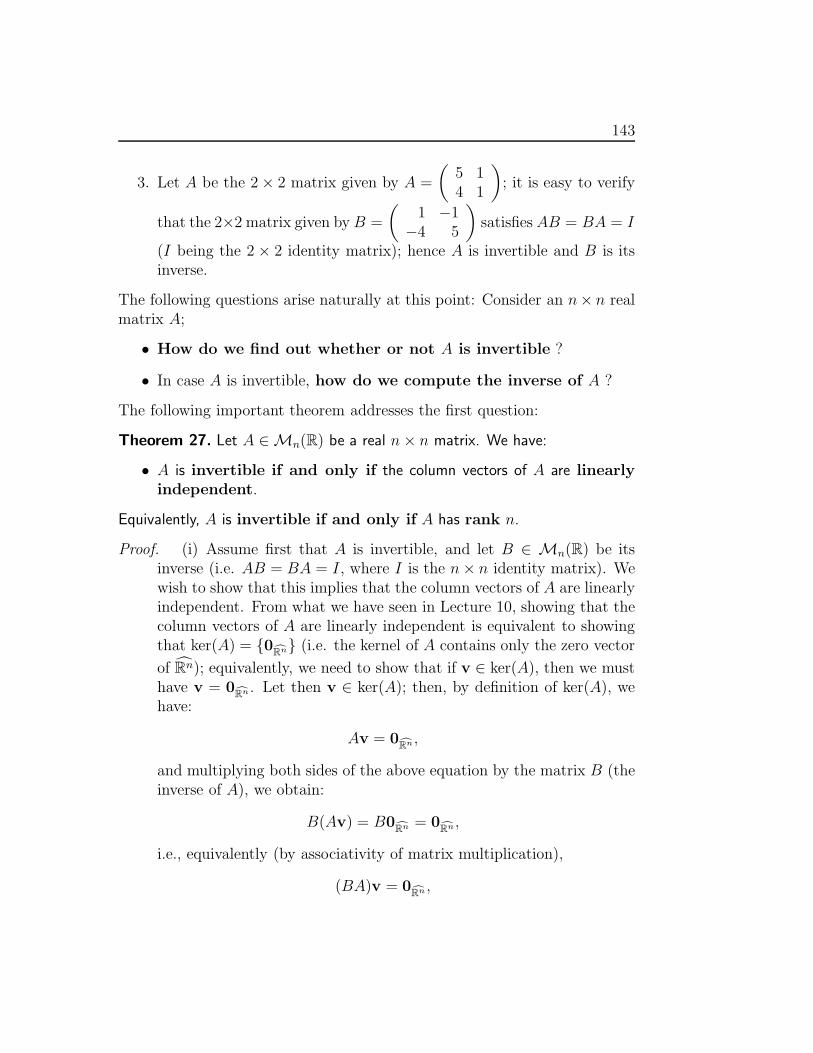
143
3. Let A be the 2 × 2 matrix given by A =
(5 14 1
); it is easy to verify
that the 2×2 matrix given by B =
(1 −1
−4 5
)satisfies AB = BA = I
(I being the 2 × 2 identity matrix); hence A is invertible and B is itsinverse.
The following questions arise naturally at this point: Consider an n× n realmatrix A;
• How do we find out whether or not A is invertible ?
• In case A is invertible, how do we compute the inverse of A ?
The following important theorem addresses the first question:
Theorem 27. Let A ∈ Mn(R) be a real n × n matrix. We have:
• A is invertible if and only if the column vectors of A are linearlyindependent.
Equivalently, A is invertible if and only if A has rank n.
Proof. (i) Assume first that A is invertible, and let B ∈ Mn(R) be itsinverse (i.e. AB = BA = I, where I is the n × n identity matrix). Wewish to show that this implies that the column vectors of A are linearlyindependent. From what we have seen in Lecture 10, showing that thecolumn vectors of A are linearly independent is equivalent to showingthat ker(A) = {0cRn} (i.e. the kernel of A contains only the zero vector
of Rn); equivalently, we need to show that if v ∈ ker(A), then we musthave v = 0cRn . Let then v ∈ ker(A); then, by definition of ker(A), wehave:
Av = 0cRn,
and multiplying both sides of the above equation by the matrix B (theinverse of A), we obtain:
B(Av) = B0cRn = 0cRn,
i.e., equivalently (by associativity of matrix multiplication),
(BA)v = 0cRn ,

144 LECTURE 13
i.e.
v = 0cRn,
since BA = I and Iv = v. Hence, we have shown that v ∈ ker(A)implies v = 0cRn . This proves that ker(A) = {0cRn}, which (by Lecture10) implies that the column vectors of A are linearly independent, asdesired.
(ii) Assume now that the column vectors of A are linearly independent;we need to show that A is then invertible. Since the column vectorsof A are assumed linearly independent, it follows that the linear mapLA : Rn → Rn defined by matrix A is one-to-one (i.e. injective);furthermore, it follows from the rank-nullity theorem that the range(i.e. image) Im(A) of matrix A is all of Rn, i.e. that the linear map LA
is onto (i.e. surjective). It follows that there exists a real n×n matrixB such that:
LB ◦ LA(v) = LA ◦ LB(v) = v, ∀v ∈ Rn,
i.e.
BA = AB = I,
where I is the n × n identity matrix. Hence, A is invertible.
Before going further, let us summarize how we can apply this last ex-tremely important theorem: Suppose you are given a real n × n matrixA; then,
• If the column vectors of A form a linearly independent familyof Rn, then A is invertible;
• If the column vectors of A form a linearly dependent family ofRn, then A is not invertible.
Let us now look at a few examples before going further:

145
1. Let I =
1 0 · · · 00 1 · · · 00 0 · · · 1
be the n×n identity matrix; we have already
seen that I is invertible (and it’s inverse is I itself). Now we know whyI is invertible: It’s n column vectors are linearly independent, as canbe easily verified (and as we have seen many times earlier!).
2. Consider the 3 × 3 real matrix A =
1 1 2
−1 1 02 3 5
; Is A invertible
? Well, by the previous theorem, we have to see whether or not thecolumn vectors of A are linearly independent. Let A;1, A;2, A;3 denotethe three column vectors of A; it is easy to see that
A;1 + A;2 − A;3 = 0cR3,
which shows that the column vectors of A are not linearly independent;hence, by the previous theorem, A is not invertible.
3. Consider the 3 × 3 real matrix A =
1 2 20 1 02 3 5
; Is A invertible ?
Again, by the previous theorem, we have to see whether or not thecolumn vectors of A are linearly independent. Let A;1, A;2, A;3 denotethe three column vectors of A; it is easy to verify that {A;1, A;2, A;3}is a linearly independent subset of R3; hence, it follows from theprevious theorem that A is invertible.
We now introduce an extremely important function of matrices, the de-terminant. Before, however, we need to introduce some notation:
Definition 18. Let A ∈ Mn(R) be a square n × n matrix. Let i, j be integers≥ 1 and ≤ n. We denote by [A]i,j the (n − 1) × (n − 1) matrix obtained fromA by deleting row i and column j.
Let us see consider a few examples:
1. Consider the real 2 × 2 matrix A =
(2 13 4
); we have:
[A]1,1 = (4), [A]1,2 = (3), [A]2,1 = (1), [A]2,2 = (2).

146 LECTURE 13
2. Consider the real 3 × 3 matrix A =
5 1 0
−1 2 37 4 1
; we have:
[A]1,1 =
(2 34 1
), [A]1,2 =
(−1 3
7 1
), [A]1,3 =
(−1 2
7 4
),
[A]2,1 =
(1 04 1
), [A]2,2 =
(5 07 1
), [A]2,3 =
(5 17 4
),
[A]3,1 =
(1 02 3
), [A]3,2 =
(5 0
−1 3
), [A]3,3 =
(5 1
−1 2
).
We are now ready to define the determinant of a square matrix:
Definition 19. Let A ∈ Mn(R) be a square n × n real matrix. The deter-minant det(A) of A is the real number defined as follows:
(i) If n = 1, i.e. A = (a) for some real number a, then det(A) = a;
(ii) If n > 1, then det(A) is recursively defined as follows:
det(A) =
n∑
j=1
(−1)1+ja1,j det([A]1,j).
Let us again consider some examples:
1. Let A =
(a bc d
)be a real 2 × 2 matrix. We have:
det(A) = (−1)1+1a det([A]1,1) + (−1)1+2b det([A]1,2)
= (−1)2a det([A]1,1) + (−1)3b det([A]1,2)
= a det((d)) − b det((c))
= ad − bc.
You should learn this identity by heart:
det(
(a bc d
)) = ad − bc.

147
2. Let now A =
a b cd e fg h i
be a real 3 × 3 matrix. We have:
det(A) = (−1)1+1a det([A]1,1) + (−1)1+2b det([A]1,2) + (−1)1+3c det([A]1,3)
= a det([A]1,1) − b det([A]1,2) + c det([A]1,3)
= a det(
(e fh i
)) − b det(
(d fg i
)) + c det(
(d eg h
))
= a(ei − fh) − b(di − fg) + c(dh − eg).
(You should definitely not try to memorize this last identity!).
We state without proof the following extremely important result:
Theorem 28. Let A ∈ Mn(R) be a real n × n matrix. We have:
• A is invertible if and only if det(A) 6= 0.
Let us recapitulate: We now have two distinct ways to establish whetheror not a given n × n matrix A is invertible:
1. Consider the column vectors A;1, A;2, · · · , A;n of A: If they are lin-early independent then A is invertible; if they are linearly depen-dent, then A is not invertible.
2. Compute det(A): If det(A) 6= 0, then A is invertible; if det(A) = 0,then A is not invertible.
The reader may wonder: Why not always use the first scheme to verifyinvertibility of a given n × n matrix ? Or why not always use the secondscheme for that purpose ? What is the use of having these two schemes (whichat the end give the same result) ? Well, in some cases, the first scheme maybe easier to apply, and in other cases, the second. Let us illustrate this ontwo examples:
1. Let A =
−1 2 1 −40 3 3 72 3 5 −31 1 2 3
; The question is: is A invertible ? To
see whether or not A is invertible, we could either:
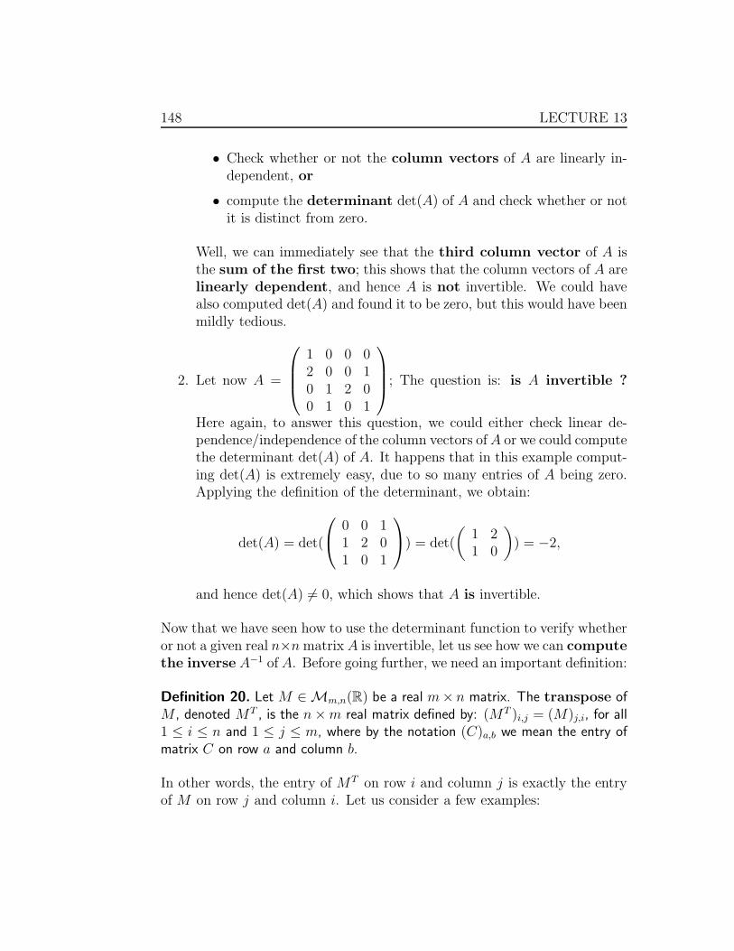
148 LECTURE 13
• Check whether or not the column vectors of A are linearly in-dependent, or
• compute the determinant det(A) of A and check whether or notit is distinct from zero.
Well, we can immediately see that the third column vector of A isthe sum of the first two; this shows that the column vectors of A arelinearly dependent, and hence A is not invertible. We could havealso computed det(A) and found it to be zero, but this would have beenmildly tedious.
2. Let now A =
1 0 0 02 0 0 10 1 2 00 1 0 1
; The question is: is A invertible ?
Here again, to answer this question, we could either check linear de-pendence/independence of the column vectors of A or we could computethe determinant det(A) of A. It happens that in this example comput-ing det(A) is extremely easy, due to so many entries of A being zero.Applying the definition of the determinant, we obtain:
det(A) = det(
0 0 11 2 01 0 1
) = det(
(1 21 0
)) = −2,
and hence det(A) 6= 0, which shows that A is invertible.
Now that we have seen how to use the determinant function to verify whetheror not a given real n×n matrix A is invertible, let us see how we can computethe inverse A−1 of A. Before going further, we need an important definition:
Definition 20. Let M ∈ Mm,n(R) be a real m× n matrix. The transpose ofM , denoted MT , is the n × m real matrix defined by: (MT )i,j = (M)j,i, for all1 ≤ i ≤ n and 1 ≤ j ≤ m, where by the notation (C)a,b we mean the entry ofmatrix C on row a and column b.
In other words, the entry of MT on row i and column j is exactly the entryof M on row j and column i. Let us consider a few examples:
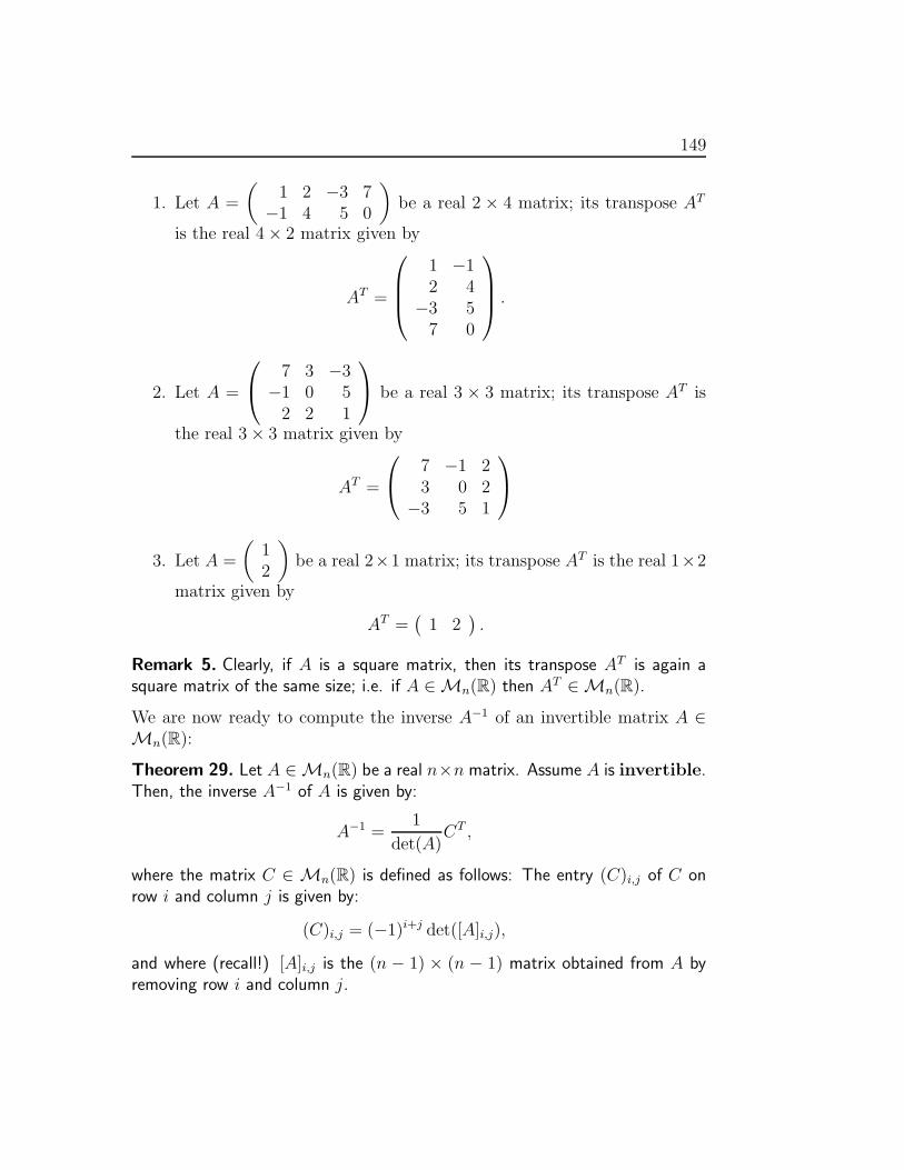
149
1. Let A =
(1 2 −3 7
−1 4 5 0
)be a real 2 × 4 matrix; its transpose AT
is the real 4 × 2 matrix given by
AT =
1 −12 4
−3 57 0
.
2. Let A =
7 3 −3
−1 0 52 2 1
be a real 3 × 3 matrix; its transpose AT is
the real 3 × 3 matrix given by
AT =
7 −1 23 0 2
−3 5 1
3. Let A =
(12
)be a real 2×1 matrix; its transpose AT is the real 1×2
matrix given by
AT =(
1 2).
Remark 5. Clearly, if A is a square matrix, then its transpose AT is again asquare matrix of the same size; i.e. if A ∈ Mn(R) then AT ∈ Mn(R).
We are now ready to compute the inverse A−1 of an invertible matrix A ∈Mn(R):
Theorem 29. Let A ∈ Mn(R) be a real n×n matrix. Assume A is invertible.Then, the inverse A−1 of A is given by:
A−1 =1
det(A)CT ,
where the matrix C ∈ Mn(R) is defined as follows: The entry (C)i,j of C onrow i and column j is given by:
(C)i,j = (−1)i+j det([A]i,j),
and where (recall!) [A]i,j is the (n − 1) × (n − 1) matrix obtained from A byremoving row i and column j.
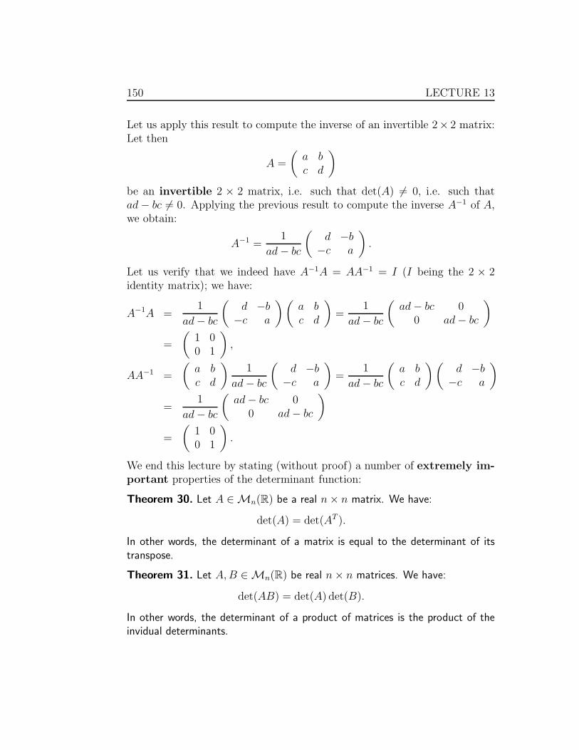
150 LECTURE 13
Let us apply this result to compute the inverse of an invertible 2× 2 matrix:Let then
A =
(a bc d
)
be an invertible 2 × 2 matrix, i.e. such that det(A) 6= 0, i.e. such thatad − bc 6= 0. Applying the previous result to compute the inverse A−1 of A,we obtain:
A−1 =1
ad − bc
(d −b
−c a
).
Let us verify that we indeed have A−1A = AA−1 = I (I being the 2 × 2identity matrix); we have:
A−1A =1
ad − bc
(d −b
−c a
) (a bc d
)=
1
ad − bc
(ad − bc 0
0 ad − bc
)
=
(1 00 1
),
AA−1 =
(a bc d
)1
ad − bc
(d −b
−c a
)=
1
ad − bc
(a bc d
) (d −b
−c a
)
=1
ad − bc
(ad − bc 0
0 ad − bc
)
=
(1 00 1
).
We end this lecture by stating (without proof) a number of extremely im-portant properties of the determinant function:
Theorem 30. Let A ∈ Mn(R) be a real n × n matrix. We have:
det(A) = det(AT ).
In other words, the determinant of a matrix is equal to the determinant of itstranspose.
Theorem 31. Let A, B ∈ Mn(R) be real n × n matrices. We have:
det(AB) = det(A) det(B).
In other words, the determinant of a product of matrices is the product of theinvidual determinants.
151
It follows from this last theorem that if A ∈ Mn(R) is invertible, thendet(A−1) = 1
det(A), i.e. the determinant of the inverse is the inverse of the
determinant. Indeed, since we have AA−1 = I (where I is the n× n identitymatrix), we obtain det(AA−1) = det(A) det(A−1) = det(I), and since wehave already computed that det(I) = 1, we obtain det(A) det(A−1) = 1,from which it follows that det(A−1) = 1
det(A).
Theorem 32. Let A ∈ Mn(R). We have, ∀i ∈ {1, 2, · · · , n}:
det(A) =
n∑
j=1
(−1)i+jai,j det([A]i,j),
where ai,j denotes the entry of A on row i and column j, and (as before) [A]i,jdenotes the (n − 1) × (n − 1) matrix obtained from A by removing row i andcolumn j.
Remark 6. Note that the definition we gave for det(A) corresponds to the aboveformula for i = 1, i.e. “expansion along the first row of A”. What the abovetheorem says is that we can compute det(A) by “expanding along any row ofA” (not just the first one).
Let now A ∈ Mn(R) be a real n × n matrix, and let us write A as
A =(
A;1 · · · A;j · · · A;n
),
where A;j denotes the jth column vector of A. If we now multiply the jth
column vector of A by some real number α (but only the jth column vectorof A), we obtain the matrix
(A;1 · · · αA;j · · · A;n
),
which has exactly the same column vectors as A except for the jth one(which has been multiplied by α. The following theorem indicates how thedeterminants of those matrices are related:
Theorem 33. For any α ∈ R, we have:
det((
A;1 · · · αA;j · · · A;n
)) = α det(
(A;1 · · · A;j · · · A;n
)).
Let now A ∈ Mn(R) be a real n × n matrix, and let α ∈ R; recall that αAis the matrix obtained by multiplying each entry of A by α. How is det(αA)related to det(A) ? The following theorem answers this question:
152 LECTURE 13
Theorem 34. ∀A ∈ Mn(R), ∀α ∈ R, we have:
det(αA) = αn det(A).
Proof. Writing A in terms of its column vectors as
A =(
A;1 · · · A;j · · · A;n
),
we obtain:
αA =(
αA;1 · · · αA;j · · · αA;n
),
and it follows from the previous theorem that
det(αA) = det((
αA;1 · · · αA;j · · · αA;n
))
= αn det((
αA;1 · · · αA;j · · · αA;n
))
= αn det(A).
Let now A ∈ Mn(R) be a real n × n matrix, which we write again in termsof its column vectors as
A =(
A;1 · · · A;i · · · A;j · · · A;n
),
where again A;i denotes the ith column vector of A and A;j its jth columnvector; what happens to the determinant if we interchange these two columnvectors, i.e. how is the determinant of the matrix
(A;1 · · · A;j · · · A;i · · · A;n
),
(which is obtained from A by interchanging column vectors i and j) relatedto the determinant of the matrix
A =(
A;1 · · · A;i · · · A;j · · · A;n
)?
The answer is given in the following theorem:
Theorem 35. Let A ∈ Mn(R) be a real n × n matrix given (in terms of itscolumn vectors) by
A =(
A;1 · · · A;i · · · A;j · · · A;n
),
153
and let A be the real n × n matrix obtained from A by interchanging columnvectors i and j, i.e.,
A =(
A;1 · · · A;j · · · A;i · · · A;n
).
Then:
det(A) = − det(A);
in other words, interchanging two column vectors changes the sign of the deter-minant.
Let now A ∈ Mn(R) be a real n × n matrix given (again in terms of itscolumn vectors) by
A =(
A;1 · · · A;j · · · A;n
),
and let v ∈ Rn be a column vector; let us add v to the jth column vector ofA (and only to that column vector); we obtain the n × n matrix
(A;1 · · · A;j + v · · · A;n
)
which differs from A only in the jth column vector. How is the determinantof this last matrix related to the determinant of A ?
Theorem 36. Let A ∈ Mn(R) be a real n × n matrix given in terms of itscolumn vectors by
A =(
A;1 · · · A;j · · · A;n
),
and let v ∈ Rn be a column vector; consider the matrix obtained from A byadding v to the jth column vector of A, i.e. the matrix
(A;1 · · · A;j + v · · · A;n
),
and let(
A;1 · · · v · · · A;n
),
be the matrix obtained by replacing the jth column vector of A by v (andkeeping all other column vectors the same as those of A). We have:
det((
A;1 · · · A;j + v · · · A;n
)) = det(
(A;1 · · · A;j · · · A;n
))
+ det((
A;1 · · · v · · · A;n
)).
154 LECTURE 13
PROBLEMS:
1. For each of the following choices for the matrix A, establish whether ornot A is invertible in the following two distinct ways:
(i) Check whether or not the column vectors of A are linearly inde-pendent.
(ii) Compute the determinant det(A) of A to see whether or not it isnon-zero.
(a) A =
(−1 2
2 1
).
(b) A =
(1 22 0
).
(c) A =
(1 20 2
).
(d) A =
(1 00 1
).
(e) A =
(0 11 0
).
(f) A =
(0 10 1
).
(g) A =
(1 10 0
).
(h) A =
(1 10 1
).
(i) A =
(1 11 1
).
(j) A =
(3 26 4
).
(k) A =
(−2 0
0 −2
).
(l) A =
(−3 0
7 0
).

155
(m) A =
(−1 2
2 −4
).
(n) A =
1 0 32 1 23 3 3
.
(o) A =
3 2 12 0 10 0 1
.
(p) A =
1 2 12 4 23 5 2
.
(q) A =
1 1 02 7 03 −3 0
.
(r) A =
1 0 01 1 01 1 1
.
(s) A =
1 0 00 1 00 0 1
.
(t) A =
1 1 10 1 10 0 1
.
(u) A =
1 1 10 1 11 0 1
.
(v) A =
2 1 37 −1 −15 −2 2
.
(w) A =
0 1 0−1 2 3−1 5 4
.

156 LECTURE 13
(x) A =
1 0 0 01 −1 0 01 2 −3 01 5 −7 −2
.
(y) A =
1 0 0 −11 −1 1 20 −2 2 31 0 0 −1
.
(z) A =
2 0 1 00 −2 5 00 1 0 21 1 −1 −1
.
Lecture 14
Study Topics
• Eigenvalues and eigenvectors of an endomorphism
• Eigenvalues and eigenvectors of a square matrix
157

158 LECTURE 14
Let V be a real vector space, and let L : V → V be a linear transformation(note here that L maps from V back to V and not to some other vectorspace; a linear mapping from a vector space back to itself is also called anendomorphism). We have the following important definition:
Definition 21. Let v ∈ V with v 6= 0 (i.e. v is not the zero vector of V); v issaid to be an eigenvector of the linear transformation L if there exists a realnumber λ such that:
L(v) = λv.
The real number λ in the above relation is called an eigenvalue of L.
We then say that v is an eigenvector of L associated to the eigenvalue λ.
Let us note the following key points before going further:
1. L is a mapping from V to V, and not from V to some other vectorspace W.
2. An eigenvector a of linear transformation L : V → V is by definitiona vector other than the zero vector 0 of V; hence, even though L(0) =0 = λ0, 0 is not considered to be an eigenvector of L.
3. For a real number λ ∈ R to be an eigenvalue of L, there must exist anon-zero vector v ∈ V such that L(v) = λv; if no such vector exists,λ cannot be an eigenvalue of L.
Let us now consider a number of examples:
1. Let V be a real vector space, and let α ∈ R be a real number. LetL : V → V be the mapping defined by L(v) = αv, ∀v ∈ V. It is easyto verify that L is a linear mapping. Furthermore (by definition of L),for any v ∈ V with v 6= 0, we have:
L(v) = αv,
which shows that v is an eigenvector of L associated to the eigen-value α. Hence, for the linear mapping L of this example, any non-zerovector in V is an eigenvector of L (associated to the eigenvalue α).

159
2. Let C∞(R; R) denote the real vector space of all functions f : R →R which are differentiable of any order (i.e. f can be differentiatedas many times as we want). Let L : C∞(R; R) → C∞(R; R) be themapping defined by:
L(f) = f ′,
where f ′ denotes the first derivative of f . It is easy to verify thatL is a linear mapping. Let us try to find an eigenvector of L. Letα ∈ R be a real number, and let f ∈ C∞(R; R) be defined by:
f(t) = eαt, ∀t ∈ R.
Let us compute L(f). We have, ∀t ∈ R:
(L(f))(t) =d
dt(eαt) = αeαt = αf(t) = (αf)(t),
which shows that
L(f) = αf.
Since f is not the zero vector of C∞(R; R), and since L(f) = αf , weconclude that f is an eigenvector of L associated to the eigenvalueα.
3. Let L : R2 → R
2 be defined by L((x, y)) = (2x, 3y) for all (x, y) ∈ R2.
It is easy to verify that L is linear. Let now v1 ∈ R2 be defined by
v1 = (1, 0). Clearly v1 is not equal to the zero vector (0, 0) of R2.
Furthermore,
L(v1) = L((1, 0)) = (2, 0) = 2(1, 0) = 2v1,
which shows that v1 is an eigenvector of L associated to the eigen-value 2.
Let now v2 ∈ R2 be defined by v2 = (0, 1). Clearly v2 is not equal to
the zero vector (0, 0) of R2. Furthermore,
L(v2) = L((0, 1)) = (0, 3) = 3(0, 1) = 3v2,
which shows that v2 is an eigenvector of L associated to the eigen-value 3.
160 LECTURE 14
Let now A ∈ Mn(R) be a real n×n matrix (note that A is a square matrix),
and consider the linear mapping LA : Rn → Rn defined by A; Note that LA
maps from Rn back to itself (this is why we chose A to be a square matrix!),and as a result, we can try to find eigenvectors and eigenvalues of LA.
• NOTE: We will just say “eigenvalue (resp. eigenvector) of A” insteadof “eigenvalue (resp. eigenvector) of LA”.
Let then λ ∈ R; Assume λ is an eigenvalue of A. This means that theremust exist a non-zero vector v ∈ Rn such that
LA(v) = λv,
i.e. (using matrix notation) such that
Av = λv.
This in turn implies that
λv − Av = 0cRn ,
i.e., that
(λI − A)v = 0cRn ,
where I denotes the n×n identity matrix. But then, this last equality meansnothing other than that v is in the kernel ker(λI −A) of the matrix λI −A.
Since v is assumed to be distinct from the zero vector of Rn and since it liesin the kernel ker(λI −A) of λI −A, it follows that ker(λI −A) must contain
more than just the zero vector of Rn! But then this means that λI − A isnot invertible (otherwise ker(λI − A) would have contained only the zero
vector of Rn), i.e. that det(λI − A) = 0 !Conversely, assume the real number λ ∈ R is such that det(λI −A) = 0; thisthen implies that the kernel ker(λI − A) of the matrix λI − A is not equalto {0cRn}, i.e. there does exist a vector v 6= 0cRn in ker(λI − A); in otherwords, we have both v 6= 0cRn and (λI − A)v = 0cRn , and this last equalityimplies Av = λv. To recapitulate: We have shown that if λ ∈ R is suchthat det(λI − A) = 0, then there exists a v ∈ Rn such that v 6= 0cRn andAv = λv; this shows that λ is an eigenvalue of A.We have therefore proved the following important theorem:

161
Theorem 37. Let A ∈ Mn(R) be a real n × n matrix. Let λ ∈ R. We have:
• λ is an eigenvalue of A if and only if det(λI − A) = 0 (where againI denotes the n × n identity matrix).
The importance of this theorem lies in that it will provide us a systematicway to compute the eigenvalues of any n × n matrix. This theorem has thefollowing useful corollary:
Theorem 38. Let A ∈ Mn(R) be a real n× n matrix. Then 0 is an eigenvalueof A if and only if A is not invertible.
Proof. 0 being an eigenvalue of A is equivalent (by the last theorem) todet(0I − A) = 0, i.e. to det(−A) = 0, i.e. to (−1)n det(A) = 0, i.e todet(A) = 0, which itself is equivalent to A being not invertible (by what wesaw in the last lecture).
Let now A ∈ Mn(R) be given by
A =
a1,1 a1,2 · · · a1,n
a2,1 a2,2 · · · a2,n...
... · · · ...an,1 an,2 · · · an,n
.
We can then write, ∀λ ∈ R:
det(λI − A) = det
λ − a1,1 −a1,2 · · · −a1,n
−a2,1 λ − a2,2 · · · −a2,n...
... · · · ...−an,1 −an,2 · · · λ − an,n
.
An explicit computation of this last determinant yields that det(λI − A)has the form:
det(λI − A) = λn + cn−1λn−1 + cn−2λ
n−2 + · · · + c2λ2 + c1λ + c0,
where the real numbers c0, c1, · · · , cn−2, cn−1 are determined by the entries ofmatrix A (i.e. by the ai,j).It is important to note the following key points:

162 LECTURE 14
1. For any real n× n matrix A, det(λI −A) is a polynomial of degreen in λ,
2. the coefficients of the polynomial det(λI − A) are determined by theentries of matrix A,
3. the coefficient of the highest order term (i.e. λn) in the polynomialdet(λI−A) is always equal to 1 (we say that the polynomial det(λI−A)is monic),
4. the roots of the polynomial det(λI − A) are exactly the eigenvaluesof A.
Due to the importance of the polynomial (in λ) defined by det(λI − A), wegive it a special name:
Definition 22. Let A ∈ Mn(R) be a real n × n matrix. The polynomial ofdegree n in λ given by det(λI − A) is called the characteristic polynomialof A.
Now we know how to compute the eigenvalues of a given matrix A ∈Mn(R); all we have to do is proceed as follows:
(i) Compute the characteristic polynomial of A,
(ii) Find the roots of the characteristic polynomial of A, i.e. find all thescalars λ which satisfy det(λI − A) = 0 ; these are the eigenvalues ofA.
Let us consider a few examples to illustrate the procedure highlighted above:
1. Let A ∈ M2(R) be given by A =
(2 11 2
); suppose we wish to find
all the eigenvalues of A. How would we proceed ? Well, as detailedabove, all we have to do is:
(i) Compute the characteristic polynomial det(λI − A) of A (whereI is the 2 × 2 identity matrix),
(ii) find the roots of that characteristic polynomial, i.e. all λ whichsatisfy det(λI − A) = 0.
163
The characteristic polynomial det(λI − A) is easily computed to be:
det(λI − A) = det(
(λ − 2 −1−1 λ − 2
))
= (λ − 2)2 − 1
= λ2 − 4λ + 3.
Note that this characteristic polynomial is, as expected, a monic poly-nomial of degree 2 (since A is 2 × 2).
The eigenvalues of A are given by solving the equation
det(λI − A) = 0,
i.e. by solving
λ2 − 4λ + 3 = 0;
we immediately find that the only solutions are given by λ = 1 andλ = 3. Hence, we conclude that the set of eigenvalues of A is given bythe set {1, 3}.
2. Let now I ∈ Mn(R) denote (as usual) the n × n identity matrix;let us try to find the eigenvalues of I. Again, as detailed above, all wehave to do is:
(i) Compute the characteristic polynomial det(λI − I) of I,
(ii) find the roots of that characteristic polynomial, i.e. all λ whichsatisfy det(λI − I) = 0.
The characteristic polynomial det(λI − I) of I is easily computed tobe:
det(λI − I) = det((λ − 1)I)
= (λ − 1)n det(I)
= (λ − 1)n,
since, as we have already seen, det(I) = 1.
The eigenvalues of I are given by solving the equation
det(λI − I) = 0,
164 LECTURE 14
i.e. by solving
(λ − 1)n = 0
we immediately find that the only solution is given by λ = 1. Hence,we conclude that the real number 1 is the only eigenvalue of the n× nidentity matrix I, i.e. the set of eigenvalues of I is given by the set {1}.
3. Let now A ∈ Mn(R) denote the n × n zero matrix (i.e. all entries ofA are zero); let us try to find the eigenvalues of A. Again, as detailedabove, all we have to do is:
(i) Compute the characteristic polynomial det(λI − A) of A,
(ii) find the roots of that characteristic polynomial, i.e. all λ whichsatisfy det(λI − A) = 0.
The characteristic polynomial det(λI − A) of A is easily computed tobe:
det(λI − A) = det(λI)
= λn det(I)
= λn.
The eigenvalues of A are given by solving the equation
det(λI − A) = 0,
i.e. by solving
λn = 0.
We immediately find that the only solution is given by λ = 0. Hence,we conclude that the real number 0 is the only eigenvalue of the n× nzero matrix A, i.e. the set of eigenvalues of A is given by the set {0}.
4. Let now A ∈ M3(R) be given by A =
a b c0 d e0 0 f
for some real
numbers a, b, c, d, e, f ; again, suppose we wish to find all the eigenvaluesof A. Again, as detailed above, all we have to do is:
165
(i) Compute the characteristic polynomial det(λI − A) of A (whereI is the 3 × 3 identity matrix),
(ii) find the roots of that characteristic polynomial, i.e. all λ whichsatisfy det(λI − A) = 0.
The characteristic polynomial det(λI − A) is easily computed to be:
det(λI − A) = det(
λ − a −b −c
0 λ − d −e0 0 λ − f
)
= (λ − a)(λ − d)(λ − f)
= λ3 − (a + d + f)λ2 + (ad + af + df)λ − adf.
Note that this characteristic polynomial is, as expected, a monic poly-nomial of degree 3 (since A is 3 × 3).
The eigenvalues of A are given by solving the equation
det(λI − A) = 0,
i.e. by solving
(λ − a)(λ − d)(λ − f) = 0
we immediately find that the only solutions are given by λ = a andλ = d, and λ = f . Hence, we conclude that the set of eigenvalues of Ais given by the set {a, d, f}.
Remark 7. Before going further, let us consider the 2 × 2 real matrix A =(0 −11 0
)and let us try to compute its eigenvalues. According to the procedure
outlined above, we begin by computing the characteristic polynomial det(λI−A)of A (where I denotes the 2 × 2 identity matrix). We obtain:
det(λI − A) = det
(λ 1−1 λ
)
= λ2 + 1.
The eigenvalues of A are then given by all the scalars λ which satisfy
det(λI − A) = 0,
166 LECTURE 14
i.e. which satisfy
λ2 + 1 = 0.
But there is no real number λ which satisfies λ2+1 = 0! Hence, we can saythat A has no real eigenvalue. On the other hand, the complex numbers iand −i are the two solutions to the above equation (recall that i2 = −1); hencewe can say that this particular matrix A has only complex eigenvalues andno real eigenvalue.In this lecture, we will restrict ourselves to n×n matrices which have only realeigenvalues.
Now that we have a “recipe” for computing all the eigenvalues of a given realn × n matrix A, how do we compute the corresponding eigenvectors ?We begin with a definition:
Definition 23. Let A ∈ Mn(R) be a real n × n matrix, and let λ ∈ R be an
eigenvalue of A. The vector subspace of Rn given by ker(λI −A) is called theeigenspace of A associated to the eigenvalue λ of A.
It is important to note the following points:
(i) ker(λI − A) is indeed a vector subspace of Rn (see the lecture on theKernel of a linear mapping).
(ii) Any non-zero vector v in ker(λI − A) is an eigenvector of A asso-ciated with eigenvalue λ; indeed, let v ∈ ker(λI − A) with v 6= 0. Wethen have
(λI − A)v = 0,
which implies
Av = λIv,
which implies
Av = λv,
and since v 6= 0, this shows that v is an eigenvector of A associatedwith eigenvalue λ.
167
These observations naturally lead us to a “recipe” for computing eigenvectorsof a given real n×n matrix A. How do we do it ? Well, as suggested above, wefirst compute all the eigenvalues of A, and then compute the eigenspace asso-ciated to each eigenvalue. Each non-zero vector in the eigenspace associatedto a given eigenvalue will be an eigenvector associated to that eigenvalue.Let us illustrate this “recipe” on an example:
1. Let A ∈ M2(R) be given by A =
(2 11 2
)(as before); we have
already computed all the eigenvalues of A, and we know that the set ofeigenvalues of A is the set {1, 3}. Let us now compute the eigenspacesassociated to each of these eigenvalues:
The eigenspace associated to the eigenvalue 1 of A is the vector sub-
space of R2 given by:
ker(1I − A) = ker(
(1 − 2 −1−1 1 − 2
)) = ker(
(−1 −1−1 −1
)),
in other words, the eigenspace of A associated to eigenvalue 1 is
nothing other than the kernel of the matrix
(−1 −1−1 −1
), and we
already know very well how to compute kernels of matrices! So let’s doit! We have:
ker(
(−1 −1−1 −1
)) = {
(xy
)∈ R2| − x − y = 0},
and therefore,
(xy
)∈ ker(
(−1 −1−1 −1
)) implies
(xy
)=
(x−x
)= x
(1−1
).
Let v1 ∈ R2 be defined by v1 =
(1−1
). The above calculation shows
that {v1} is a generating set for the eigenspace of A associated witheigenvalue 1; furthermore, it is easy to verify that {v1} is a linearlyindependent set. Hence, (v1) is a basis for the eigenspace of Aassociated to the eigenvalue 1, and we conclude therefore that that
168 LECTURE 14
eigenspace is one-dimensional. In particular, v1 itself is an eigenvectorof A associated with eigenvalue 1. Let us verify this last claim: Clearlyv1 6= 0, and we have
Av1 =
(2 11 2
) (1−1
)=
(2 − 11 − 2
)=
(1−1
)= v1 = 1v1,
as expected.
Let us now compute the eigenspace of A associated to the eigenvalue 3of A. The eigenspace associated to the eigenvalue 3 of A is the vector
subspace of R2 given by:
ker(3I − A) = ker(
(3 − 2 −1−1 3 − 2
)) = ker(
(1 −1−1 1
)),
in other words, the eigenspace of A associated to eigenvalue 3 is
nothing other than the kernel of the matrix
(1 −1−1 1
); again,
this is something we know very well how to compute! We have:
ker(
(1 −1−1 1
)) = {
(xy
)∈ R2|x − y = 0},
and therefore,
(xy
)∈ ker(
(1 −1−1 1
)) implies
(xy
)=
(xx
)= x
(11
).
Let v2 ∈ R2 be defined by v2 =
(11
). The above calculation shows
that {v2} is a generating set for the eigenspace of A associated witheigenvalue 3; furthermore, it is easy to verify that {v2} is a linearlyindependent set. Hence, (v2) is a basis for the eigenspace of Aassociated to the eigenvalue 3, and we conclude therefore that thateigenspace is one-dimensional. In particular, v2 itself is an eigenvectorof A associated with eigenvalue 3. Let us verify this last claim: Clearlyv2 6= 0, and we have
Av2 =
(2 11 2
) (11
)=
(2 + 11 + 2
)=
(33
)= 3v2,
as expected.
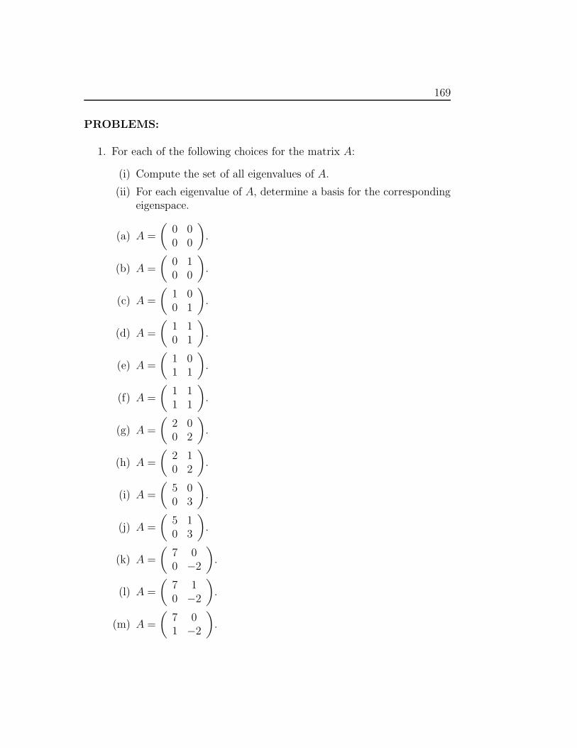
169
PROBLEMS:
1. For each of the following choices for the matrix A:
(i) Compute the set of all eigenvalues of A.
(ii) For each eigenvalue of A, determine a basis for the correspondingeigenspace.
(a) A =
(0 00 0
).
(b) A =
(0 10 0
).
(c) A =
(1 00 1
).
(d) A =
(1 10 1
).
(e) A =
(1 01 1
).
(f) A =
(1 11 1
).
(g) A =
(2 00 2
).
(h) A =
(2 10 2
).
(i) A =
(5 00 3
).
(j) A =
(5 10 3
).
(k) A =
(7 00 −2
).
(l) A =
(7 10 −2
).
(m) A =
(7 01 −2
).

170 LECTURE 14
(n) A =
(3 11 3
).
(o) A =
(3 22 3
).
(p) A =
(3 14 3
).
(q) A =
(3 19 3
).
(r) A =
(3 10 3
).
(s) A =
(3 20 3
).
(t) A =
1 0 00 1 00 0 1
.
(u) A =
1 1 00 1 10 0 1
.
(v) A =
1 0 10 1 00 0 1
.
(w) A =
1 1 10 1 10 0 1
.
(x) A =
2 0 00 5 00 0 7
.
(y) A =
2 1 00 5 10 0 7
.
(z) A =
2 0 10 5 00 0 7
.
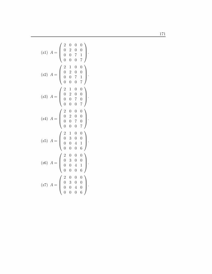
171
(z1) A =
2 0 0 00 2 0 00 0 7 10 0 0 7
.
(z2) A =
2 1 0 00 2 0 00 0 7 10 0 0 7
.
(z3) A =
2 1 0 00 2 0 00 0 7 00 0 0 7
.
(z4) A =
2 0 0 00 2 0 00 0 7 00 0 0 7
.
(z5) A =
2 1 0 00 3 0 00 0 4 10 0 0 6
.
(z6) A =
2 0 0 00 3 0 00 0 4 10 0 0 6
.
(z7) A =
2 0 0 00 3 0 00 0 4 00 0 0 6
.