IMES DISCUSSION PAPER SERIES

INSTITUTE FOR MONETARY AND ECONOMIC STUDIES

BANK OF JAPAN

C.P.O BOX 203 TOKYO

100-8630 JAPAN

You can download this and other papers at the IMES Web site:

http://www.imes.boj.or.jp

Do not reprint or reproduce without permission.

Approximation of Interest Rate Derivatives’ Prices by Gram-Charlier Expansion and Bond Moments

Keiichi Tanaka, Takeshi Yamada and Toshiaki Watanabe

Discussion Paper No. 2005-E-16

NOTE: IMES Discussion Paper Series is circulated in

order to stimulate discussion and comments. Views

expressed in Discussion Paper Series are those of

authors and do not necessarily reflect those of

the Bank of Japan or the Institute for Monetary

and Economic Studies.

IMES Discussion Paper Series 2005-E-16November 2005

Approximation of Interest Rate Derivatives’ Prices byGram-Charlier Expansion and Bond Moments

Keiichi Tanaka*, Takeshi Yamada**, Toshiaki Watanabe***

AbstractIn this paper, we develop easily implemented approximations of the prices ofseveral interest rate derivatives. We study swaptions, constant maturity swaps(“CMS”), and CMS options. For swaption prices, we approximate swaption pricesunder one forward measure by using a Gram-Charlier expansion. This expansion isan orthogonal decomposition of a density function in additive form and involvesbond moments in the coefficients. Hence, the swaptions price can be approximatedeasily and accurately. Higher-order approximations yield very accurate pricesenough to price each transaction, and lower-order approximations are suitable forportfolio evaluation and risk management. In addition, we approximate CMS ratesby using bond moments. We also approximate prices of CMS options bycombining the two methods.

Keywords: Gram-Charlier expansion, bond moment, swaption, constant maturityswap, convexity adjustment

JEL classification Numbers: G13

* Graduate School of Economics, Kyoto University(E-mail: tanakak@econ.kyoto-u.ac.jp)

** Institute for Monetary and Economic Studies, Bank of Japan(E-mail: takeshi.yamada@boj.or.jp)

*** Institute for Monetary and Economic Studies, Bank of Japan(E-mail: toshiaki.watanabe@boj.or.jp)

An earlier version of this paper was entitled “A Simple Formulation of Swaption Prices byGram-Charlier Expansion”. We are grateful for constructive discussions with Masaaki Kijima,Carl Chiarella, and Atsushi Kawai. For helpful comments, we also thank the staff of theInstitute for Monetary and Economic Studies (IMES), the Bank of Japan (BOJ), and seminarparticipants at Kyoto University, IMES, NFA 2005, JAFEE 2005, and the 2005 DaiwaInternational Workshop. This research was partly carried out while Tanaka was at the IMESand Watanabe was at the Tokyo Metropolitan University. Financial support from the DaiwaChair of Graduate School of Economics, Kyoto University is gratefully acknowledged byTanaka. The views expressed in this paper are those of the authors and do not necessarilyreflect those of the BOJ or the IMES. The authors are responsible for any remaining errors.

Contents

I Introduction . . . . . . . . . . . . . . . . . . . . . . . . . . . . . . . . . . . 1II Approximating Interest Rate Derivative Price by using a Gram–Charlier

Expansion . . . . . . . . . . . . . . . . . . . . . . . . . . . . . . . . . . . . 2A The valuation of a swaption . . . . . . . . . . . . . . . . . . . . . . . 2B The Gram–Charlier expansion . . . . . . . . . . . . . . . . . . . . . 3C Swaption . . . . . . . . . . . . . . . . . . . . . . . . . . . . . . . . . 6D Constant Maturity Swap (CMS) . . . . . . . . . . . . . . . . . . . . 8E CMS Option . . . . . . . . . . . . . . . . . . . . . . . . . . . . . . . 10

III Affine Term Sructure Models and the Greeks . . . . . . . . . . . . . . . . 11IV Numerical examples . . . . . . . . . . . . . . . . . . . . . . . . . . . . . . 14

A Parameters . . . . . . . . . . . . . . . . . . . . . . . . . . . . . . . . 14B Swaption prices based on the Gaussian model . . . . . . . . . . . . . 17C Swaption prices based on the CIR model . . . . . . . . . . . . . . . . 19D Convexity adjustments for CMS rates . . . . . . . . . . . . . . . . . 19

V Conclusion . . . . . . . . . . . . . . . . . . . . . . . . . . . . . . . . . . . 23References . . . . . . . . . . . . . . . . . . . . . . . . . . . . . . . . . . . . . . . 24A Affine term structure models . . . . . . . . . . . . . . . . . . . . . . . . . 25

A A0(J) Gaussian Model . . . . . . . . . . . . . . . . . . . . . . . . . . 25B AJ(J) CIR Model . . . . . . . . . . . . . . . . . . . . . . . . . . . . 25

I. Introduction

Many financial institutions hold large portfolios of interest rate derivatives transactions.In many cases, the maturity of these transactions is long and the number of contracts ina portfolio will not decrease in a short time. Therefore, an efficient calculation methodis needed, not only for pricing specific transaction, but also for evaluation and riskmanagement of the portfolio. An efficient calculation method has two features. (1) itis not computer-intensive for the valuation of a portfolio. (2) it can handle many typesof products, including swaps, caps, and constant maturity swaps (“CMS”), within thesame model to avoid inconsistent valuations among products. In this paper, we developeasily implemented approximations of the prices of several interest rate derivatives. Westudy swaptions, CMS and CMS options.

Jamshidian (1989) derived an exact analytical pricing formula for options on couponbonds with a one-factor model. However, except for the forward swap measure approachof Jamshidian (1997), a closed formula for swaptions has not been obtained in multi-factor models due to the difficulty of identifying the exercise boundary with respect tothe underlying factors. Brace (1997) proposed a rank-r approximation method for swap-tion prices in the LIBOR market model. Singleton and Umantsev (2002) linearized theexercise boundary (or the corresponding swap rate) with respect to the state variablesunder essentially affine term structure models. An innovative approximation method forswaptions was proposed by Collin-Dufresne and Goldstein (2002) (hereafter, “CDG”).They developed an approximation method under Gaussian and CIR (Cox-Ingersoll-Ross,[1985]) models by approximating the density function. For both models, their approachproduces accurate approximation and fast calculation compared with Monte Carlo sim-ulations.

For swaption prices, we simplify and complement the approach of CDG to obtaina swaption pricing formula that can be easily implemented for particular types of termstructure model. We use a Gram–Charlier expansion of the density function of theunderlying swap at the swaption expiry under the forward measure associated with theexpiry. The coefficients of the series are expressed by the cumulants or, equivalently, bythe moments. This approach works, as CDG explained, when the moments are calculatedanalytically, as in, e.g., affine term structure models and Gaussian Heath–Jarrow–Mortonmodels (see, e.g., Musiela and Rutkowski [2005]). Our formula is closely related to severalresults based on the Malliavin calculus and the Fourier transform. This is because theGram–Charlier expansion is obtained by using a Fourier inversion of the characteristicfunction. It is also a version of the Wiener Chaos expansion. Note that we approximatethe density function of a swap value that takes both positive and negative values. Hence,it is not subject to the criticism that the distribution of a price that takes only positivevalues cannot be approximated by normal distributions.

Following CDG, we expand the density function of the underlying swap. However,whereas CDG carried out their calculations under many forward measures associated withthe swaption expiry and cash-flow timing, we use only one forward measure associatedwith the swaption expiry. Thus, our formula is easier to implement and more accurate.Our numerical study of affine term structure models confirms that our method yields bet-ter approximations than that of CDG. We conclude that higher-order approximationsare sufficiently accurate for pricing specific transactions, while lower-order approxima-tions are speedily obtained and suitable for portfolio evaluation and risk management.

1

However, the error depends on the model parameters, such as the level of the yield curveor the mean reversion speed.

In addition, we approximate CMS rates by using moments of bonds (“bond mo-ments”), and approximate the prices of CMS options by combining our two methods.Benhamou (2000) derived an approximation of the convexity adjustment of a CMS ratefor lognormal zero coupon models by using a Wiener Chaos expansion. The literatureon convexity adjustment is cited in Benhamou (2000). Calculating the convexity adjust-ment for a CMS rate is difficult because the swap value and duration, each of which is alinear combination of bond prices, are correlated. Hence, bond moments can be used toprice the convexity adjustment. To approximate CMS option prices, we combine the twomethods, the Gram–Charlier expansion and bond moments. Although there is a paral-lelism in the form of results between this paper and Benhamou (2000), our approach canbe easily applied to wider classes of models.

The rest of this paper is organized as follows. In Section II, we develop an approxima-tion method by using a Gram–Charlier expansion. We present formulae for swaptions,CMS, and option on CMS based on the cumulants of the underlying swap. In SectionIII, we describe affine term structure models and derive bond moments and Greeks. InSection IV, we perform numerical calculations for affine term structure models. SectionV concludes the paper.

II. Approximating Interest Rate Derivative Price by using

a Gram–Charlier Expansion

A. The valuation of a swaption

We denote by P (t, T ) the time-t price of a zero coupon bond with a maturity date of T .(Ω,F , P ) is a probability space with a J-dimensional standard Brownian motion W . Weassume that tradable assets comprise zero coupon bonds and a money-market account,and that there is a risk-neutral measure, Q, with the Brownian motion W Q.

We consider a swaption with the expiry T0 and the fixed rate K (per payment andnotional amount) during a period [T0, TN ]. We fix the relevant dates, T0 < T1 < · · · < TN ,which are set at regularly spaced time intervals, with δ = Ti − Ti−1 for all i. The valueSV (t) of the underlying swap at time t is given by

SV (t) =

−P (t, T0) + δK∑N

i=1 P (t, Ti) + P (t, TN ), for the receiver’s swaption,

P (t, T0) − δK∑N

i=1 P (t, Ti) − P (t, TN ), for the payer’s swaption,

≡N

∑

i=0

aiP (t, Ti), (1)

where ai is the amount of cash flow at time Ti. Following from the usual discussion aboutno-arbitrage and the change of measure, the swaption value, SOV (t), at time t is firstevaluated under the risk-neutral measure Q, and then converted to the expected value

2

of the gain from exercising under the T0-forward measure, P T0 , as follows

SOV (t) = EQ[

e− T0t rsds max(SV (T0), 0) | Ft

]

= P (t, T0)ET0

[

1SV (T0)>0SV (T0) | Ft

]

= P (t, T0)

∫ ∞

0xf (x)dx, (2)

where f is the density function of the swap value SV at the expiry date T0 under theT0-forward measure conditioned by Ft.

B. The Gram–Charlier expansion

Following Stuart and Ord (1987), we derive the Gram–Charlier expansion and show itsrelationship to the Edgeworth expansion. As shown below, the Edgeworth expansionis obtained by using the inverse Fourier transform of the characteristic function in amultiplicative form. The Gram–Charlier expansion is further expanded and reorderedas an orthogonalized series of the Edgeworth expansion in additive form. The Gram–Charlier expansion is more useful for many practical purposes.

We define the Chebyshev–Hermite polynomial as Hn(x) = (−1)nφ(x)−1Dnφ(x) withH0(x) = 1, where D = d

dx and φ(x) = (2π)−1/2 exp(−x2/2). 1 The Chebyshev–Hermitepolynomials have the orthogonal property

∫ ∞−∞ Hm(x)Hn(x)φ(x)dx = δmnn! with respect

to the Gaussian measure, ν, which has a standard normal distribution, N(0, 1). As shownin equation (3) below, by using the properties of the Chebyshev–Hermite polynomials,the Gram–Charlier expansion is an orthogonal decomposition with Hnφn of a densityfunction that has coefficients qn, each of which depends on a given set of cumulants.

Proposition 1. Assume that a random variable Y has the density function f and has

cumulants ck (k ≥ 1), all of which are finite and known. Then the followings hold.

(i) f can be expanded as follows

f(x) =

∞∑

n=0

qn√c2

Hn

(x − c1√c2

)

φ(x − c1√

c2

)

, (3)

where qn =1

n!E[Hn

(Y − c1√c2

)

]

=

1, if n = 0,0, if n = 1, 2,∑[n/3]

m=1

∑∗∗ ck1···ckm

m!k1!···km!

(

1√c2

)n, if n ≥ 3,

(4)

∑∗∗means

∑

k1+···+km=n,ki≥3

.

1We use Hn for the Chebyshev–Hermite polynomial, which should not be confused with the Hermite

polynomial, Hn(x), defined by Hn(x) = (−1)nex2

Dne−x2

= 2n/2Hn(√

2x). By definition,

H0(x) = 1, H1(x) = x, H2(x) = x2 − 1, H3(x) = x

3 − 3x, H4(x) = x4 − 6x

2 + 3,

H5(x) = x5 − 10x

3 + 15x, H6(x) = x6 − 15x

4 + 45x2 − 15, H7(x) = x

7 − 21x5 + 105x

3 − 105x.

3

(ii) for any a ∈ R,

E[1Y >a] = N(c1 − a√

c2

)

+

∞∑

k=3

(−1)k−1qkHk−1

(c1 − a√c2

)

φ(c1 − a√

c2

)

,

E[1Y >aY ] = c1N(c1 − a√

c2

)

+√

c2φ(c1 − a√

c2

)

+

∞∑

k=3

(−1)kqk

(

−aHk−1

(c1 − a√c2

)

+√

c2Hk−2

(c1 − a√c2

)

)

φ(c1 − a√

c2

)

.

Proof. The characteristic function GY of a random variable Y is defined by the Fouriertransform of f as

GY (t) =

∫ ∞

−∞eitxf(x)dx = eitc1

∫ ∞

−∞ei√

c2tx√c2f(c1 +√

c2x)dx. (5)

On the other hand, by the definitions of the cumulants, this can be expressed as

GY (t) = exp[

∞∑

k=1

ck

k!(it)k

]

= eitc1

∫ ∞

−∞ei√

c2tx exp[

∞∑

k=3

(−1)kck

k!

( D√c2

)k]

φ(x)dx. (6)

This is because, for any sequence an, it follows that

exp(

−c2

2t2 +

∞∑

n=1

an(−i√

c2t)n)

=

∫ ∞

−∞ei√

c2tx exp(

∞∑

n=1

anDn)

φ(x)dx.

We further expand the integrand of equation (6) by using the Taylor expansion. We thenreorder the terms as follows

exp[

∞∑

k=3

(−1)kck

k!

( D√c2

)k]

φ(x)

=(

1 +

∞∑

m=1

1

m!

[

∞∑

k=3

(−1)kck

k!

( D√c2

)k]m)

φ(x)

=(

1 +

∞∑

m=1

1

m!

∑

k1,··· ,km≥3

(−1)k1+···+kmck1 · · · ckm

k1! · · · km!

( D√c2

)k1+···+km)

φ(x)

=(

1 +∑∗ ck1 · · · ckm

m!k1! · · · km!

( 1√c2

)nHn(x)

)

φ(x),

where∑∗means

∑∞n=3

∑[n/3]m=1

∑

k1+···+km=n,ki≥3. We use the relationship Hn(x)φ(x) =(−1)nDnφ(x) in the last equality. Then, equation (6) can be written as

eitc1

∫ ∞

−∞ei√

c2txφ(x)dx + eitc1

∫ ∞

−∞ei√

c2tx∑∗ ck1 · · · ckm

m!k1! · · · km!

( 1√c2

)nHn(x)φ(x)dx. (7)

By using the inverse Fourier transforms of both equations (5) and (7) and by changingthe relevant variable, we obtain the following Gram–Charlier expansion around the mean

4

2:

f(x) =1√c2

φ(x − c1√

c2

)

+1√c2

∑∗ ck1 · · · ckm

m!k1! · · · km!

( 1√c2

)nHn

(x − c1√c2

)

φ(x − c1√

c2

)

.

The proof of (ii) is straightforward by using (i) and the properties of Chebyshev–Hermitepolynomials.

The Gram–Charlier expansion may be interpreted as the Wiener Chaos expansionof f /φ ∈ L2(R,B(R), ν), where f(x) =

√c2f(c1 +

√c2x) is the density function of the

standardized random variable (Y − c1)/√

c2. The Wiener Chaos expansion states thatthe Chebyshev–Hermite polynomials form a complete orthonormal system in the Hilbertspace, L2(R,B(R), ν) (see Nualart [1995], p.7). The advantages of the Gram–Charlierexpansion are that it is written in additive form and the coefficients qn are easily expressedby the given cumulants as follows 3

q0 = 1, q1 = q2 = 0, q3 =c3

3!c3/22

, q4 =c4

4!c22

,

q5 =c5

5!c5/22

, q6 =c6 + 10c2

3

6!c32

, q7 =c7 + 35c3c4

7!c7/22

. (8)

The cumulants, cj , can be calculated from the moments, µj, around zero. 4

In the proof of Proposition 1, the inverse Fourier transforms of both equations (5)and (6) yield the Edgeworth expansion

f(x) =1√c2

exp[

∞∑

k=3

(−1)kck

k!Dk

]

φ(x − c1√

c2

)

. (9)

However, this multiplicative form is not useful for approximating option prices. Hence,we require an additive form. Both the Gram-Charlier and the Edgeworth expansionsare equivalent (have the same value) when the summation is taken over infinite terms,

2For the density function of a standardized random variable, an expansion around zero f(x) = ∞

k=0 qkHk(x)φ(x), where qk = 1k!

E[Hk(Y )] = [k/2]

l=0(−1)l

l!(k−2l)!2lE[Y k−2l], is known as a Gram–Charlier

series of type A (Stuart and Ord [1987]).3In this context, it is well known that 3!q3 represents skewness and 4!q4 represents the excess kurtosis.4See Stuart and Ord (1987). For example,

c1 = µ1, c2 = µ2 − µ21, c3 = µ3 − 3µ1µ2 + 2µ

31,

c4 = µ4 − 4µ1µ3 − 3µ22 + 12µ

21µ2 − 6µ

41,

c5 = µ5 − 5µ1µ4 − 10µ2µ3 + 20µ21µ3 + 30µ1µ

22 − 60µ

31µ2 + 24µ

51,

c6 = µ6 − 6µ1µ5 − 15µ2µ4 + 30µ21µ4 − 10µ

23 + 120µ1µ2µ3 − 120µ

31µ3

+ 30µ32 − 270µ

21µ

22 + 360µ

41µ2 − 120µ

61,

c7 = µ7 − 7µ1µ6 − 21µ2µ5 − 35µ3µ4 + 140µ1µ23 − 630µ1µ

32 + 210µ1µ2µ4

− 1260µ21µ2µ3 + 42µ

21µ5 + 2520µ

31µ

22 − 210µ

31µ4 + 210µ

22µ3 + 840µ

41µ3

− 2520µ51µ2 + 720µ

71.

5

but the truncated sum may lead to differences between them. However, in many prac-tical applications, the finite sum is the same after a further approximation is made onthe Edgeworth expansion. The approximation based on the Gram–Charlier expansionignores the “orthogonalized moments”, qn, in the context of equation (8), whereas theapproximation based on the Edgeworth expansion ignores the higher cumulants, cn.

C. Swaption

Suppose that we know the j-th cumulant, cj , of the underlying swap value at the expiry T0

under the forward measure P T0 that is associated with the option expiry with conditionFt. We set the following: Cj = cjP (t, T0)

j and qk = qk(c1, . . . , ck) = qk(C1, . . . , Ck),which is calculated from equation (8). Then, the swaption value is obtained from equation(2) as

SOV (t)

= P (t, T0)ET0

[

1SV (T0)>0SV (T0) | Ft

]

= P (t, T0)[

c1N( c1√

c2

)

+√

c2φ( c1√

c2

)

+√

c2φ( c1√

c2

)

∞∑

k=3

(−1)kqkHk−2

( c1√c2

)

]

= C1N( C1√

C2

)

+√

C2φ( C1√

C2

)

+√

C2φ( C1√

C2

)

∞∑

k=3

(−1)kqkHk−2

( C1√C2

)

. (10)

In particular, the truncated sum of equation (10) yields an approximation of the swaptionvalue.

Proposition 2. The swaption value is approximated as

SOV (t) ≈ C1N( C1√

C2

)

+√

C2φ( C1√

C2

)

+√

C2φ( C1√

C2

)

L∑

k=3

(−1)kqkHk−2

( C1√C2

)

. (11)

We refer to this expression as the L-th order approximated price, GCL.

Hence, the calculation of the swaption is reduced to the value of cumulants cj of theunderlying swap or the swap moments

Mm(t) = ET0

[

(SV (T0))m | Ft

]

= ET0

[(

N∑

i=0

aiP (T0, Ti))m

| Ft

]

=∑

0≤i1,... ,im≤N

ai1 · · · aimµT0(t, T0, Ti1 , . . . , Tim), (12)

where T0 is the expiry date of the swaption, T1, . . . , Tm are the coupon payment datesand

µT (t, T0, T1, . . . , Tm) ≡ ET[

m∏

i=1

P (T0, Ti) | Ft

]

(13)

6

is the bond moments under the T -forward measure with T ≥ T0. As shown subsequently,µT0(t, T0, T1, . . . , Tm) can be calculated analytically for particular classes of interestrate models.

It is worth mentioning that other approaches based on the Edgeworth expansion canbe used to reach the same conclusion as that implied by equation (11). For a givenforward measure, the two expansions, the Gram–Charlier expansion and the Edgeworthexpansion, are numerically equivalent and the truncated sums are numerically equivalentwhen an appropriate approximation is made.

The asymptotic expansion approach is developed by using Malliavin calculus (see,e.g., Kunitomo and Takahashi [2001]). Essentially, it used a third-order Edgeworthexpansion and an approximation as

f(x) ≈ 1√c2

exp[−c3

3!D3

]

φ(x − c1√

c2

)

≈ 1√c2

[

1 − c3

3!D3

]

φ(x − c1√

c2

)

=1√c2

[

1 +c3

3!(√

c2)3H3

(x − c1√c2

)]

φ(x − c1√

c2

)

.

It seems that the numerical performance of Kunitomo and Takahashi (2001) is similar toours. Kawai (2003) approximates swaptions by using an asymptotic expansion approachin the LIBOR market model. In existing studies, the swaption value is often decomposedinto weighted cash-flow values based on the exercise probabilities under the forwardmeasures associated with the cash-flow timing,

SOV (t) =

N∑

i=0

aiP (t, Ti)ETi

[

1SV (T0)>0 | Ft

]

. (14)

When calculating the probability of ending up in-the-money under the forward measure,CDG used a seventh-order Edgeworth expansion. They ignored terms higher than D7 ina further expanded series by a Taylor expansion of the exponential,

f(x) ≈ 1√c2

exp[

7∑

k=3

(−1)kck

k!Dk

]

φ(x − c1√

c2

)

≈ 1√c2

(

1 +7

∑

k=3

(−1)kck

k!Dk +

1

2

((c3

3!D3

)2 − 2c3

3!

c4

4!D3D4

)

)

φ(x − c1√

c2

)

=1√c2

(

1 + q3H3 + q4H4 + q5H5 + q6H6 + q7H7

)

φ(x − c1√

c2

)

,

where Hk = Hk

(

x−c1√c2

)

. This approximation of the density is exactly the same as ours

when L = 7. Furthermore, CDG found that c6 and c7 were negligible in equation (8)relative to c2

3 and c3c4, respectively. Thus, q6 and q7 are represented by low-degreecumulants, which reduces computational time.

The truncated Edgeworth expansion,

1√c2

exp[

L∑

k=3

(−1)kck

k!Dk

]

φ(x − c1√

c2

)

7

makes full use of the properties of a finite set of cumulants, c1, . . . , cL. CDG’s recalcula-tion of q6 and q7 with c6 = c7 = 0 may be regarded as a way of using as much informationon c3, c4, and c5 as possible. However, the truncated Gram–Charlier expansion,

L∑

n=0

qn√c2

Hn

(x − c1√c2

)

φ(x − c1√

c2

)

,

does not fully reflect the properties of the cumulants c3, . . . , cL because of the truncation.This is a disadvantage of the orthogonal decomposition and may explain why a higher-order approximation does not necessarily yield a better approximation than a lower-orderapproximation.

Equations (2) and (14) are equivalent. However, in the applications, their computa-tional efficiency and approximation errors differ. When the swaption value is expressed asequation (2), we work under the T0-forward measure, P T0 . On the other hand, CDG pro-posed taking the set of forward measures PTii and working with equation (14). In thiscase, appropriate formulae must be used to calculate probability ETi

[

1SV (T0)>0 | Ft

]

for each measure. Using equation (2) rather than equation (14) reduces the time takento compute the moments because there are fewer underlying measures. In terms of ap-proximation error, one would conjecture that equation (14) might accumulate the errorof each expectation. The main difference between CDG’s approach and ours is the choiceof the measures. Thus, CDG’s results may differ from ours. In the section on numericalexamples, we compare the results of the two approaches.

D. Constant Maturity Swap (CMS)

In this subsection, we demonstrate the another usefulness of the bond moments in anapproximation of the convexity adjustment of a CMS rate. A CMS is a swap contractbetween two parties to exchange a fixed rate and a floating rate, which has a reference ratethat is a swap rate with a specified time to maturity. The fixed rate to be exchanged ona CMS is called the CMS rate. Similar products to CMS include 15-year floating couponJapanese Government Bonds (“JGB”) with a 10-year JGB coupon 5, and Long-TermPrime Rate swaps with a reference rate that is a coupon of a 5-year bank debenture.

We fix the relevant dates, T0 < T1 < . . . < Tn < . . . < Tn+m, which are set atregularly spaced time intervals with δ = Ti − Ti−1 for all i. We consider a CMS to betraded at time t < T0 for the exchange of a fixed rate CMS(t) with the observed swaprates for a maturity of τ = mδ in arrears during the period [T0, Tn]. The fixing datesare Ti (i = 0, . . . , n − 1) and the payment dates are Ti+1. By the usual discussion, thetime-t value of the floating rate amount that is fixed at time Ti and settled at time Ti+1

is written as

δP (t, Ti+1)ETi+1 [S(Ti, Ti, τ) | Ft],

where S(u, Ti, τ) is the forward swap rate for the period [Ti, Ti + τ ] at time u,

S(u, Ti, τ) =P (u, Ti) − P (u, Ti + τ)

δ∑i+m

j=i+1 P (u, Tj).

5This kind of bond, whose coupon is linked to a yield or a coupon rate of Government bonds with apredetermined time to maturity, is called a constant maturity treasury (“CMT”).

8

The fixed rate on the CMS is given by

CMS(t) =

∑ni=1 P (t, Ti+1)E

Ti+1 [S(Ti, Ti, τ) | Ft]∑n

i=1 P (t, Ti). (15)

(See Musiela and Rutkowski [2005].)The expectation of the swap rate, ETi+1 [S(Ti, Ti, τ) | Ft], is close to the forward swap

rate S(t, Ti, τ). They coincide if the swap rate is a martingale under the forward measure.Otherwise, a difference between them exists and it is called the convexity adjustment ina broad sense (bCA). 6 Hence, it is sufficient to consider the bCA of the single-periodCMS rate; n = 1, and

bCA = ET1 [S(T0, T0, τ) | Ft] − S(t, T0, τ).

Now let t ≤ u ≤ T0. We consider a receiving swap with a coupon rate of S(t, T0, τ)for a period of [T0, Tm]. Recall that the time-u swap value is given by

SV (u) = δ

m∑

j=1

P (u, Tj)(S(t, T0, τ) − S(u, T0, τ)).

We define the duration (or basis point value) of the swap Dur(u) as follows

Dur(u) = δ

m∑

j=1

P (u, Tj). (16)

Given that

S(u, T0, τ) = S(t, T0, τ) +

∑mj=1 P (u, Tj)(S(u, T0, τ) − S(t, T0, τ))

∑mj=1 P (u, Tj)

= S(t, T0, τ) − SV (u)

Dur(u), (17)

by taking expectations of both sides, we have

bCA = −ET1 [SV (T0)Dur(T0)−1 | Ft]. (18)

A major problem in evaluating the CMS is that no general analytical expression existsfor the expectation of SV (T0)Dur(T0)

−1. We propose a simple approximation of thisexpectation based on bond moments. We make use of the fact that both the swapvalue and the duration are affine functions of bond prices. Let us denote by D(t) =δ∑m

j=1 P (t, Tj)/P (t, T0) the forward duration of the swap. This would be close to theconditional mean of a random variable, Dur(T0). We can approximate the stochasticduration by a first- or second-order deterministic duration as follows

Dur(T0)−1 =

D(t)−1

1 + Dur(T0)−D(t)D(t)

≈

1D(t)

(

2 − Dur(T0)D(t)

)

(for the first-order approx.),

1D(t)

(

3 − 3Dur(T0)D(t) +

(

Dur(T0)D(t)

)2)

(for the second-order approx.).

(19)6bCA for the LIBOR is zero because a forward LIBOR of maturity date Ti+1 is a martingale under

the Ti+1-forward measure S(t, Ti, δ) = ETi+1 [S(Ti, Ti, δ) | Ft].

9

Note that (1 + x)−1 ≈ 1 − x (the first-order approximation) and (1 + x)−1 ≈ 1 − x + x2

(the second-order approximation). Then, for the first-order approximation, we obtainthe following result, which can be modified for the second-order approximation. Bondmoments allow us to calculate the convexity adjustment easily.

Proposition 3. The first-order approximation of the single-period CMS rate is given by

ET1 [S(T0, T0, τ) | Ft] ≈ S(t, T0, τ) −m

∑

j=0

aj

(2µT1(t, T0, Tj)D(t)

− δm

∑

k=1

µT1(t, T0, Tj , Tk)D(t)2

)

,

where 7

aj =

−1 if j = 0,δS(t, T0, τ) if 0 < j < m,

1 + δS(t, T0, τ) if j = m.

Note that the bCA represents convexity adjustment with different timings for theobservation, T0, and the payment, T1. We can consider a convexity adjustment with thesame timing and call it the convexity adjustment in a narrow sense (nCA). 8 By notingthat ET0 [SV (T0) | Ft] = 0, equation (18) can be decomposed into two terms, as follows

bCA = −ET1 [SV (T0)Dur(T0)−1 | Ft]

= −CovT0 [SV (T0),Dur(T0)−1 | Ft]

+(

ET0 [SV (T0)Dur(T0)−1 | Ft] − ET1 [SV (T0)Dur(T0)

−1 | Ft])

.

The first term, −CovT0t [SV (T0),Dur(T0)

−1](= −ET0 [SV (T0)Dur(T0)−1 | Ft]), is the

nCA, which represents adjustment based on the same timing for the observation andthe payment. The remaining term in the bracket, ET0 [· · · ]−ET1 [· · · ], represents timingadjustment (TA). This is because the observation, T0, and the settlement, T1, havedifferent timing.

E. CMS Option

The methods we have discussed so far are useful. The approximated price of an optioncontract on a CMS swap can be obtained by combining the two methods to approximate aswaption price by the Gram–Charlier expansion (in Section II.C) and a convexity adjust-ments of a CMS rate with bond moments (in Section II.D). We present the approximatedprice of a floor of a single period CMS.

CMS options are often incorporated in structured products such as callable bondand capped floater. The 15-year JGB incorporates a floor for the CMT rate since thecoupon is set as the maximum of either zero or the current 10-year JGB coupon minussome constant alpha.9 Therefore, the valuation of these options is of great interest topractitioners.

7aj (j = 0, . . . , m) is the cash flow at time Tj , used to represent the swap with the fixed rate ofS(t, T0, τ ).

8Convexity adjustment for bond yields is an example of nCA.9In the 15-year JGB issued on 2005 July, alpha is set at 0.95 percent; i.e., the floor is struck at 0.95

percent.

10

A swap rate is observed on T0. The observed swap is assumed to start on T0 and isassumed to include the coupon exchanges on T1, . . . , Tm with δ = Ti −Ti−1 and τ = mδ.The strike rate of the floor is K and the payment of the floor is made on T1. The valueis then given by

CMSFloor(t) = EQ[

exp(

−∫ T1

trsds

)

δ max(K − ST0 , 0) | Ft

]

= δP (t, T1)ET1

[

max(K − S(T0, T0, τ), 0) | Ft

]

.

From equations (17) and (19), we can approximate the observed swap rate as

S(T0, T0, τ) = S(t, T0, τ) − SV (T0)

Dur(T0)

≈ S(t, T0, τ) − SV (T0)( 2

D(t)− 1

D(t)2Dur(T0)

)

Thus, we obtain an approximated price of the CMS floor as

CMSFloor(t)

≈ δP (t, T1)ET1

[

max(

K − S(t, T0, τ) +2

D(t)SV (T0) −

1

D(t)2SV (T0)Dur(T0), 0

)

| Ft

]

.

This can be approximated further by using the Gram–Charlier expansion and the bondmoments. The positive part of the cash flow at the expiry consists of three parts: (i)a constant, K − S(t, T0, τ); (ii) a linear combination of bond prices, 2

D(t)SV (T0); and

(iii) a quadratic combination of bond prices− 1D(t)2

SV (T0)Dur(T0). Thus, while it is

straightforward to calculate the swap moments, this requires higher order bond momentsbecause of the quadratic terms.

III. Affine Term Sructure Models and the Greeks

Our methods for approximating swaptions and CMS prices are independent of any modelif bond moments can be obtained analytically or numerically. If a specific model withstate variables is applied to the underlying model, we may be able to calculate theGreeks of the swaptions with respect to the state variables based on the approximation.Examples include not only affine term structure models (ATSMs), but also Gaussianquadratic term structure models (see, e.g., Ahn et al. [2002]) and Gaussian Heath–Jarrow–Morton models. In this section, we introduce ATSMs, on which the numericalexamples in Section IV are based. Then, we evaluate the deltas of a swaption price forATSMs.

In an ATSM, the bond price is expressed in the form of an exponentially affinefunction,

P (t, T ) = exp(A(t, T ) + B(t, T )>X(t)), (20)

of a vector of factors (or state variables), X = (X1, . . . ,XJ )>, which follows dX(t) =µX(X(t), t)dt+ σX (X(t), t)dWQ(t) under Q. Duffie and Kan (1996) characterized affine

11

models. Under certain conditions, expressing the bond price in the above form is equiv-alent to assuming that the short rate r, the drift term µX , and σXσX

> are affine func-tions of X. It is sufficient to restrict our attention to the case in which r and X satisfyr(t) = δ0 + δX

>X(t), and dX(t) = KQ(θQ − X(t))dt + ΣD(X(t))dWQ(t), respectively,where δ0, α ∈ R, δX , θQ, β ∈ R

J , and KQ ∈ RJ×J , D(X(t)) is the diagonal matrix

D(X(t)) = diag[

√

α1 + β1>X(t), . . . ,

√

αJ + βJ>X(t)

]

, and Σ ∈ RJ×J is a matrix such

that ΣΣ> is a covariance matrix.The Feynman–Kac formula yields the following system of ordinary differential equa-

tions:

∂

∂tA(t, T ) = −(KQθQ)>B(t, T ) − 1

2

J∑

j=1

(Σ>B(t, T ))j2αj + δ0, A(T, T ) = 0,

∂

∂tB(t, T ) = KQ>

B(t, T ) − 1

2

J∑

j=1

(Σ>B(t, T ))j2βj + δX , B(T, T ) = 0. (21)

This system can be solved in a closed form for special cases and can be solved numericallyin many other cases. An important characteristic of ATSMs is that the zero rate, R(t, T ),and the instantaneous forward rate, f(t, T ), for a maturity date of T at time t, are affinefunctions of X. They are given by

R(t, T ) = −(T − t)−1(A(t, T ) + B(t, T )>X(t)),

f(t, T ) = −∂A(t, T )

∂T− ∂B(t, T )

∂TX(t).

As is the bond price, the moments are exponentially affine, and are of the form

µT (t, T0, T1, . . . , Tm) =exp(M(t) + N(t)>X(t))

P (t, T ),

where M(t) = M(t, T, T0, T1, . . . , Tm) and N(t) = N(t, T, T0, T1, . . . , Tm) satisfy thesame system of ordinary differential equations

∂

∂tM(t) = −(KQθQ)>N(t) − 1

2

J∑

j=1

(Σ>N(t))j2αj + δ0,

∂

∂tN(t) = KQ>

N(t) − 1

2

J∑

j=1

(Σ>N(t))j2βj + δX . (22)

The terminal conditions are

M(T0) =m

∑

i=1

A(T0, Ti) + A(T0, T ), N(T0) =m

∑

i=1

B(T0, Ti) + B(T0, T ).

These follow from the Feynman–Kac formula. In Gaussian-type and CIR-type mod-els, there are explicit solutions for A,B,M, and N . These solutions are given in theAppendix. Given these formulae, it is straightforward to apply the Gram–Charlier ex-pansion for swaption prices.

12

Using these functional forms, it is easy to show that the swaption delta with respectto the initial value Xi(0) is given by

∂SOV (0)

∂Xi(0)=

1

2C2

∂C2

∂Xi(0)SOV (0)

+( ∂C1

∂Xi(0)− C1

2C2

∂C2

∂Xi(0)

)(

N(C1√C2

) +

∞∑

k=3

(−1)k−1qkHk−1(C1√C2

)φ(C1√C2

))

+√

C2

∞∑

k=3

(−1)k∂qk

∂Xi(0)Hk−2(

C1√C2

)φ(C1√C2

). (23)

The Greeks with respect to other parameters can be obtained in a similar way.

13

IV. Numerical examples

In this section, we give numerical examples using two ATSMs (a three-factor Gaussianmodel and a two-factor CIR model), following CDG. We compute the (receiver’s) swap-tion prices of various strikes by using a Gram–Charlier expansion and compare themwith prices calculated by a Monte Carlo simulation with respect to accuracy and com-putational burden. In addition, approximations of CMS rates are investigated in eachmodel.

A. Parameters

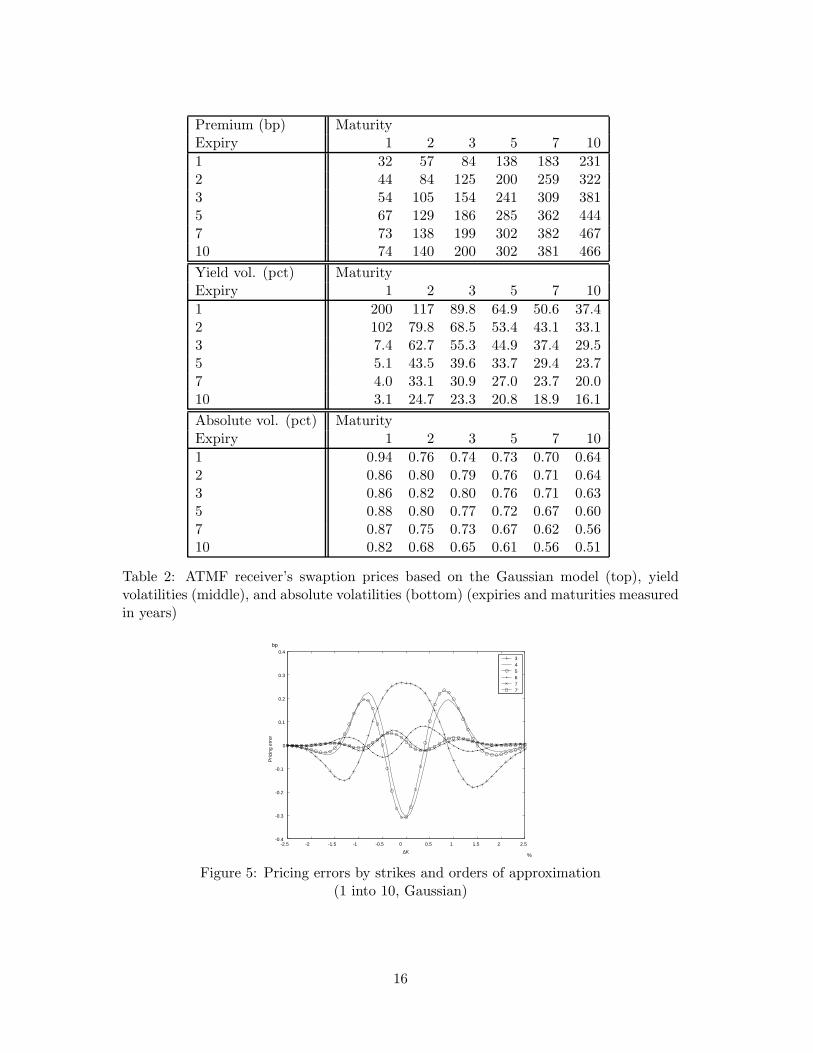
Parameters are selected as shown in Table 1, so that the induced rates approximatelyfit observed Japanese Yen data. One of the reasons for choosing the Japanese Yen datais its closeness to the non-positive area for interest rates, which will distinguish variousnumerical performances. Figure 1 shows three series of Japanese Yen swap rates, theobserved yield curve in markets on 23 February 2005, and the yield curves implied by thetwo models. Table 2 shows the option data implied by the Gaussian model, which includethe at-the-money-forward (ATMF) receivers’ swaption prices in basis points (bp) and twotypes of volatilities in percents (pct), which we will explain shortly. The reader can graspthe level of swaption prices before we discuss the accuracy of the approximation.

As there is no standard pricing formula for interest rate derivatives, a swaption istraded by two parties after they agree on the premium (swaption price). Volatilityis treated simply as a reference for their negotiations. Usually, swaption prices arequoted in units of basis points by market traders and brokers. There are two typesof reference volatility. Yield volatility is used when using Black’s formula to value anoption. Yield volatility is also known as relative volatility because of its form. The othertype of volatility, absolute volatility, is yield volatility multiplied by the ATMF rate.Yield volatilities are more widely used than absolute volatilities among practitionersin financial markets. However, a benefit of the absolute volatility is that its intuitivemeaning roughly represents the annual standard deviation of a particular swap rate tobe observed. Other advantages are that the surface of the absolute volatilities is relativelyflat and there is little dependence on the level of yield curve. We consider a one-year intoa 10-year swaption (“1 into 10”) as a reference because our parameters imply a relativelylow cumulative absolute volatility compared with other expiries and maturities.

First, we check the approximated distributions of 10-year swap rates (and values) oneyear later. Figure 2 shows the distribution of the swap rates. Figures 3 and 4 show thedensity function of the value of a 10-year receiving swap one year later, for the Gaussianand CIR models, respectively. The swap rate is set to the ATMF rate. In the caseof the Gram–Charlier expansion, the density function of the swap value is obtained byusing equation (3) up to a particular order. For the Monte Carlo method, the densityis obtained by simulation with exact distributions at expiry for both the Gaussian andCIR models. Note that the Gram–Charlier expansion provides a good approximation forthe Gaussian model. However, in the CIR model, it overweights the probability aroundthe lower rates by one percent more than the ATMF rate and underweights it aroundthe higher rates.

14

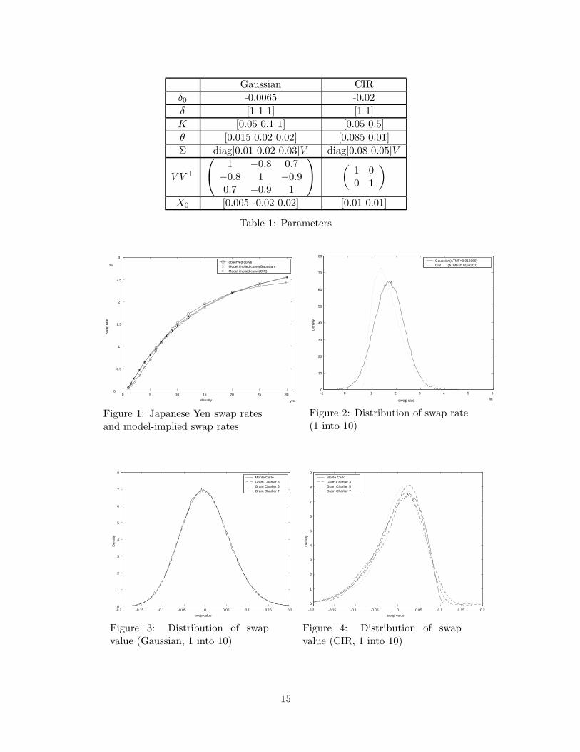
Gaussian CIR

δ0 -0.0065 -0.02

δ [1 1 1] [1 1]

K [0.05 0.1 1] [0.05 0.5]

θ [0.015 0.02 0.02] [0.085 0.01]

Σ diag[0.01 0.02 0.03]V diag[0.08 0.05]V

V V >

1 −0.8 0.7−0.8 1 −0.90.7 −0.9 1

(

1 00 1

)

X0 [0.005 -0.02 0.02] [0.01 0.01]

Table 1: Parameters

0 5 10 15 20 25 300

0.5

1

1.5

2

2.5

3

Maturity

Sw

ap r

ate

observed curveModel implied curve(Gaussian)Model implied curve(CIR)

%

yrs

Figure 1: Japanese Yen swap ratesand model-implied swap rates

-1 0 1 2 3 4 5 6 0

10

20

30

40

50

60

70

80

swap rate

Den

sity

Gaussian(ATMF=0.016989)CIR (ATMF=0.0168207)

%

Figure 2: Distribution of swap rate(1 into 10)

-0.2 -0.15 -0.1 -0.05 0 0.05 0.1 0.15 0.20

1

2

3

4

5

6

7

8

swap value

Den

sity

Monte CarloGram Charlier 3Gram Charlier 5Gram Charlier 7

Figure 3: Distribution of swapvalue (Gaussian, 1 into 10)

-0.2 -0.15 -0.1 -0.05 0 0.05 0.1 0.15 0.2

0

1

2

3

4

5

6

7

8

9

swap value

Den

sity

Monte CarloGram Charlier 3Gram Charlier 5Gram Charlier 7

Figure 4: Distribution of swapvalue (CIR, 1 into 10)

15

Premium (bp) MaturityExpiry 1 2 3 5 7 10

1 32 57 84 138 183 2312 44 84 125 200 259 3223 54 105 154 241 309 3815 67 129 186 285 362 4447 73 138 199 302 382 46710 74 140 200 302 381 466

Yield vol. (pct) MaturityExpiry 1 2 3 5 7 10

1 200 117 89.8 64.9 50.6 37.42 102 79.8 68.5 53.4 43.1 33.13 7.4 62.7 55.3 44.9 37.4 29.55 5.1 43.5 39.6 33.7 29.4 23.77 4.0 33.1 30.9 27.0 23.7 20.010 3.1 24.7 23.3 20.8 18.9 16.1

Absolute vol. (pct) MaturityExpiry 1 2 3 5 7 10

1 0.94 0.76 0.74 0.73 0.70 0.642 0.86 0.80 0.79 0.76 0.71 0.643 0.86 0.82 0.80 0.76 0.71 0.635 0.88 0.80 0.77 0.72 0.67 0.607 0.87 0.75 0.73 0.67 0.62 0.5610 0.82 0.68 0.65 0.61 0.56 0.51

Table 2: ATMF receiver’s swaption prices based on the Gaussian model (top), yieldvolatilities (middle), and absolute volatilities (bottom) (expiries and maturities measuredin years)

-2.5 -2 -1.5 -1 -0.5 0 0.5 1 1.5 2 2.5 -0.4

-0.3

-0.2

-0.1

0

0.1

0.2

0.3

0.4

∆K

Pric

ing

erro

r

345677’

bp

%

Figure 5: Pricing errors by strikes and orders of approximation(1 into 10, Gaussian)

16

B. Swaption prices based on the Gaussian model

In this subsection, we analyze the pricing errors of the swaption prices in the Gaussianmodel. Figure 5 illustrates pricing errors for a one-year into a 10-year swaption withseveral strike rates (from ATMF−2.5% to ATMF+2.5%). The horizontal axis representsthe difference, ∆K, between the strike rate and the ATMF rate. The pricing error iscalculated as the approximated price equation (11) based on the Gram–Charlier expan-sion (“GC price”) minus the price from the Monte Carlo simulation (“MC price”). GC7′

is obtained from GC7 with the sixth and seventh cumulants being set equal to 0 inequation (8). 10 The MC price is obtained by simulating 400 million times (20 millionruns multiplied by 20 to calculate MC error) with the negative correlation technique,and using Gaussian distribution of state variables at the expiry to avoid the discretizingerror. The standard error is of the order of 10−6 for a one-year into 10-year swaption.

All pricing errors are within 0.3 bp for GC3, GC4, and GC5, and within 0.1 bp forGC6, GC7′, and GC7. The results of GC7′ are similar to those of GC7. Note that thehigher-order approximations (GC4 and GC5) do not necessarily produce more accurateprices than lower order approximations (GC3). The reason is that the Gram–Charlierexpansion is an orthogonal expansion. Table 3 shows the GC prices and MC prices usedin Figure 5. Note that for the ATMF swaption (C1 = 0), there are no contributionsfrom the odd-order term because H2k+1(0) = 0. In addition, the contribution of eachterm of the odd (even) order behaves like an odd (even) function of ∆K because of theproperties of the Chebyshev–Hermite polynomials.

Similar wave patterns of pricing errors are reported for other combinations of expiriesand maturities in Figures 6 and 7. The magnitudes of the fluctuations depend on theexpiry and maturity. Nevertheless, the errors for various strikes in five-year into 10-yearswaptions based on GC3 are, at most, 2 bp. Due to the higher absolute volatilities ofshorter maturities (one-year into 5-year swaptions) compared with one-year into 10-yearswaptions, the option delta is higher for the same distance from the ATMF rate, so thatthe shape of Figure 6 is a zoomed-in picture of a certain part of Figure 5. A similarexplanation applies to Figure 7. This is because the standard deviation of a swap rateat the expiry T grows at the order

√T when the absolute volatility is constant. Figure 8

illustrates pricing errors for ATMF swaptions based on a seventh-order approximation.This figure shows that most pricing errors for ATMFs are within 1 bp.

Table 4 shows the calculation time for each method based on using Visual C in a 2.4GHz Pentium 4 CPU. The time for the Gram–Charlier expansion increases substantiallywith the order of the approximation and the maturity of the underlying swaps. This isdue to the associated increase in the number of terms in the summation.

By considering the accuracy and the computational time, we conclude that a higherorder approximation GC7′ yields very accurate prices enough to price a specific transac-tion, and that a lower order one GC3 attains good approximation in a very short timeso that it is suitable for the portfolio evaluation and the risk management. However,the level of the accuracy depends on the model parameters. One should note that wecompare the pricing errors of several approximation orders by using the same modelparameters. It is obvious that the error depends on the model parameters such as thelevel of the yield curve or the mean reversion speed.

10CDG use the same method as GC7′ to calculate the probabilities of ending in in-the-money underseveral relevant forward measures.

17

∆K -1% -0.5% 0% 0.5% 1%

3rd 12.600 68.438 230.926 535.646 945.868

4th 12.849 68.311 230.353 535.482 946.112

5th 12.847 68.237 230.353 535.558 946.130

6th 12.692 68.187 230.691 535.532 945.930

7′th 12.662 68.277 230.674 535.440 945.964

7th 12.652 68.278 230.691 535.435 945.955

MC 12.673 68.237 230.660 535.455 945.933

Table 3: GC prices and MC prices (bp)

-2.5 -2 -1.5 -1 -0.5 0 0.5 1 1.5 2 2.5-0.08

-0.06

-0.04

-0.02

0

0.02

0.04

0.06

0.08

∆K

Pric

ing

erro

r

3577’

bp

%

Figure 6: 1 into 5

-2.5 -2 -1.5 -1 -0.5 0 0.5 1 1.5 2 2.5-4

-3

-2

-1

0

1

2

3

4

∆K

Pric

ing

erro

r

3577’

bp

%

Figure 7: 5 into 10

2

4

6

8

10

2

4

6

8

100

0.2

0.4

0.6

0.8

1

1.2

maturityexpiry

Pric

ing

erro

r

yrs

yrs

bp

Figure 8: Pricing errors for ATMF (Gaussian, GC7)

1 into 5 ATMF 1 into 7 ATMF 1 into 10 ATMF

GC3 <0.000 <0.000 <0.000GC5 <0.000 0.031 0.156GC7′ <0.000 0.031 0.156GC7 0.063 0.438 3.453

MC(20million) 78.266 90.766 109.531

Table 4: Calculation times (sec., Gaussian)

18

C. Swaption prices based on the CIR model

It is important for practitioners to recognize the pattern and the level of the pricing errorsbefore implementing our approach. As expected, the CIR model has larger standarderrors from the Monte Carlo simulation and poorer approximations than those of theGaussian model, by about one digit. However, the main features are similar to those ofthe Gaussian model.

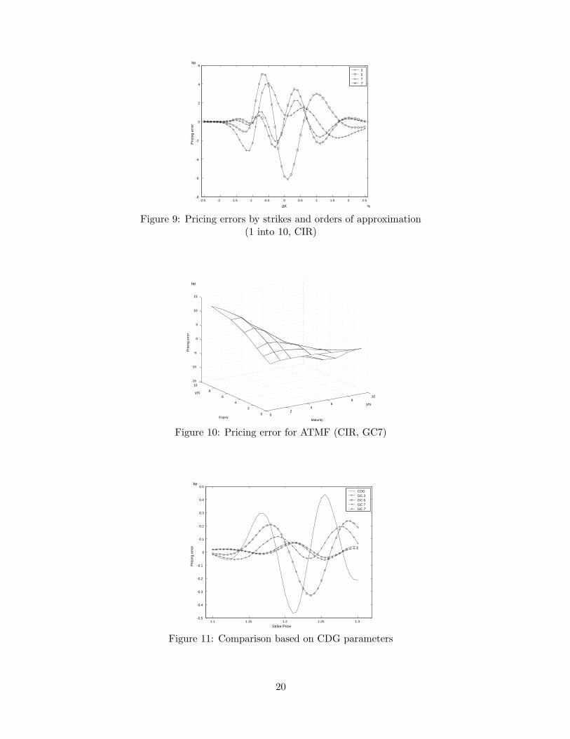
Figure 9 shows the pricing errors for one-year into 10-year swaptions from the CIRmodel. The corresponding figure for the Gaussian model is Figure 5. For the CIR model,the MC price is obtained by simulating 100 million times (5 million runs multiplied by20) by using noncentral chi-squared distributions of the state variables at the expiry toavoid the discretizing error. The basic features of the pricing errors of the CIR modellook similar to those of the Gaussian. The pricing errors are no more than 4 bp basedon GC3 and are about 2 bp based on GC7. Figure 10 shows the pricing errors from theATMF based on a seventh-order approximation. It seems that these errors for the CIRmodel are not at critical levels for the practitioners’ purposes in their daily activities,such as pricing and risk management. Calculation times are similar for the CIR andGaussian models. Therefore, the conclusion from the Gaussian model also applies to theCIR model.

As mentioned in footnote 10, CDG use the same method used for GC7′ to calculatethe probabilities of being in-the-money under several relevant forward measures. Figure11 compares the performance of the CDG approach to our approach for coupon-bondoption prices (a two-year option on 12-year bond) by using the same parameters usedby CDG. This figure indicates that our approach is better than that of CDG. Especially,difference between GC7′ and CDG shows accumulated pricing error due to the numberof forward measures. Again, accuracy depends on the model parameters. The order ofthe errors are quite different between Figures 9 and 11 since the pricing error for theCIR model will be smaller if the underlying yield is higher.

D. Convexity adjustments for CMS rates

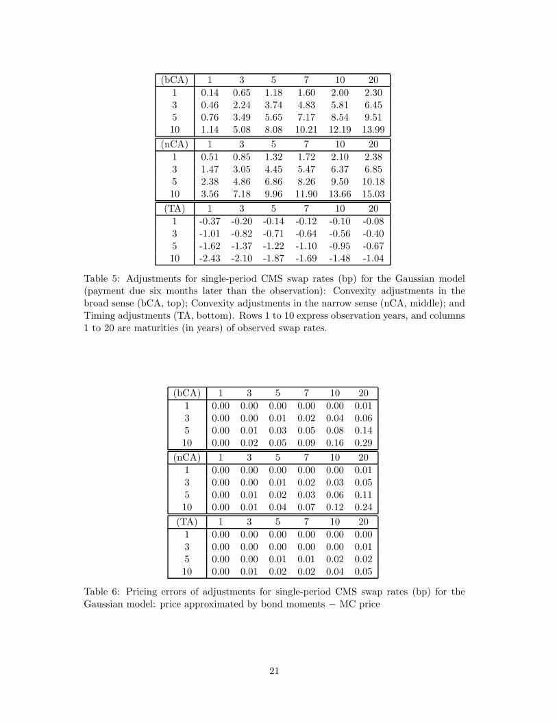
In this subsection, we investigate how accurately our approximation methods with bondmoments calculate the convexity adjustments of CMS rates. The convexity adjustments(bCA, nCA, and TA) of one-period CMS rates under the Gaussian model are calculatedby the Monte Carlo method, as shown in Table 5, to grasp the magnitudes. The longerthe time to the observation or the longer the maturity of the observed swaps, the biggerthe adjustments are. The pricing errors are reported in Tables 6, 7, and 8 for the Gaussianwith the first-order approximation, the CIR with the first-order approximation, and theCIR with the second-order approximation, respectively.

The Gaussian first-order approximation performs well. The pricing errors are, atmost, 0.29 bp for the CA in a broad sense, 0.24 bp for the CA in a narrow sense, and0.05 bp for the timing adjustment (Table 6). The CIR first-order approximation does notperform well, as Table 7 shows. The second-order approximation reduces the errors fromTable 7 by roughly half, so that they are relatively small (see Table 8). Our methods arepractical.

19

-2.5 -2 -1.5 -1 -0.5 0 0.5 1 1.5 2 2.5-8

-6

-4

-2

0

2

4

6

∆K

Pric

ing

erro

r

3577’

%

bp

Figure 9: Pricing errors by strikes and orders of approximation(1 into 10, CIR)

02

46

810

0

2

4

6

8

10-15

-10

-5

0

5

10

15

MaturityExpiry

Pric

ing

erro

r

bp

yrs

yrs

Figure 10: Pricing error for ATMF (CIR, GC7)

1.1 1.15 1.2 1.25 1.3-0.5

-0.4

-0.3

-0.2

-0.1

0

0.1

0.2

0.3

0.4

0.5

Pric

ing

erro

r

CDGGC 3GC 5GC 7GC 7’

bp

Strike Price

Figure 11: Comparison based on CDG parameters

20

(bCA) 1 3 5 7 10 20

1 0.14 0.65 1.18 1.60 2.00 2.303 0.46 2.24 3.74 4.83 5.81 6.455 0.76 3.49 5.65 7.17 8.54 9.5110 1.14 5.08 8.08 10.21 12.19 13.99

(nCA) 1 3 5 7 10 20

1 0.51 0.85 1.32 1.72 2.10 2.383 1.47 3.05 4.45 5.47 6.37 6.855 2.38 4.86 6.86 8.26 9.50 10.1810 3.56 7.18 9.96 11.90 13.66 15.03

(TA) 1 3 5 7 10 20

1 -0.37 -0.20 -0.14 -0.12 -0.10 -0.083 -1.01 -0.82 -0.71 -0.64 -0.56 -0.405 -1.62 -1.37 -1.22 -1.10 -0.95 -0.6710 -2.43 -2.10 -1.87 -1.69 -1.48 -1.04

Table 5: Adjustments for single-period CMS swap rates (bp) for the Gaussian model(payment due six months later than the observation): Convexity adjustments in thebroad sense (bCA, top); Convexity adjustments in the narrow sense (nCA, middle); andTiming adjustments (TA, bottom). Rows 1 to 10 express observation years, and columns1 to 20 are maturities (in years) of observed swap rates.

(bCA) 1 3 5 7 10 20

1 0.00 0.00 0.00 0.00 0.00 0.013 0.00 0.00 0.01 0.02 0.04 0.065 0.00 0.01 0.03 0.05 0.08 0.1410 0.00 0.02 0.05 0.09 0.16 0.29

(nCA) 1 3 5 7 10 20

1 0.00 0.00 0.00 0.00 0.00 0.013 0.00 0.00 0.01 0.02 0.03 0.055 0.00 0.01 0.02 0.03 0.06 0.1110 0.00 0.01 0.04 0.07 0.12 0.24

(TA) 1 3 5 7 10 20

1 0.00 0.00 0.00 0.00 0.00 0.003 0.00 0.00 0.00 0.00 0.00 0.015 0.00 0.00 0.01 0.01 0.02 0.0210 0.00 0.01 0.02 0.02 0.04 0.05

Table 6: Pricing errors of adjustments for single-period CMS swap rates (bp) for theGaussian model: price approximated by bond moments − MC price

21

(bCA) 1 3 5 7 10 20

1 -0.00 -0.01 -0.03 -0.05 -0.07 -0.113 -0.03 -0.13 -0.26 -0.40 -0.58 -0.915 -0.08 -0.33 -0.66 -0.99 -1.42 -2.1910 -0.24 -0.98 -1.88 -2.77 -3.90 -5.94

(nCA) 1 3 5 7 10 20

1 -0.00 -0.02 -0.03 -0.05 -0.07 -0.123 -0.03 -0.13 -0.27 -0.41 -0.60 -0.945 -0.08 -0.35 -0.69 -1.03 -1.48 -2.2810 -0.25 -1.04 -2.00 -2.94 -4.15 -6.30

(TA) 1 3 5 7 10 20

1 0.00 0.00 0.00 0.00 0.00 0.003 0.00 0.00 0.01 0.01 0.02 0.035 0.00 0.01 0.03 0.04 0.06 0.0910 0.02 0.06 0.12 0.18 0.24 0.36

Table 7: Pricing errors of adjustments for single-period CMS swap rates (bp) for theCIR model (first-order approximation)

(bCA) 1 3 5 7 10 20

1 0.00 -0.00 -0.00 -0.01 -0.01 -0.023 -0.00 -0.01 -0.04 -0.08 -0.14 -0.305 -0.01 -0.05 -0.12 -0.24 -0.42 -0.8910 -0.03 -0.19 -0.50 -0.89 -1.53 -3.09

(nCA) 1 3 5 7 10 20

1 0.00 -0.00 -0.00 -0.01 -0.01 -0.023 -0.00 -0.01 -0.04 -0.08 -0.14 -0.315 -0.01 -0.05 -0.13 -0.25 -0.44 -0.9310 -0.03 -0.20 -0.53 -0.94 -1.61 -3.25

(TA) 1 3 5 7 10 20

1 0.00 0.00 0.00 0.00 0.00 0.003 0.00 0.00 0.00 0.00 0.00 0.015 0.00 0.00 0.00 0.01 0.02 0.0310 0.00 0.01 0.03 0.05 0.08 0.16

Table 8: Pricing errors of adjustments for single-period CMS swap rates (bp) for theCIR model (second-order approximation)

22

V. Conclusion

We have developed easy-to-use approximation methods for pricing several interest ratederivatives by using the Gram–Charlier expansion and by using bond moments. Approx-imation accuracy depends on the underlying model, the detailed characteristics of theproducts, and the model parameters. From numerical studies for swaption prices, ourmethod yields smaller pricing errors than the method used by Collin-Dufresne and Gold-stein (2002). We conclude that a higher order approximation GC7′ yields very accurateprices enough to price a specific transaction, and that a lower order one GC3 attains goodapproximation in a very short time so that it is suitable for the portfolio evaluation andthe risk management. Using bond moments to calculate the convexity adjustments ofconstant maturity swap rates is novel and the approximation method performs well. Wealso derive an approximated option price on CMS rates by combining the two methods.These approximations can be applied to CMT products such as 15-year floating couponJGB.

23

References

[1] Ahn, D., R. Dittmar and A.R. Gallant “Quadratic Term Structure Models: Theoryand Evidence,” Review of Financial Studies, 15, 2002, pp. 243-288.

[2] Benhamou, E. “Pricing Convexity Adjustment with Wiener Chaos,” Working paper,London School of Economics, 2000.

[3] Brace, A. “Rank-2 Swaption Formulae,” Working paper, University of New SouthWales, 1997.

[4] Collin-Dufresne, P., and R.S. Goldstein “Pricing Swaptions Within an Affine Frame-work,” Journal of Derivatives, 10, 2002, pp. 1-18.

[5] Cox, J. C., J. E. Ingersoll and S. A. Ross, “A Theory of the Term Structure of InterestRates, Econometrica, 53, 1985, pp. 385-407.

[6] Duffie, D., and R. Kan “A Yield Factor Model of Interest Rates,” Mathematical

Finance, 6, 1996, pp. 379-406.

[7] Jamshidian, F. “An Exact Bond Option Pricing Formula,” Journal of Finance, 44,1989, pp. 205-209.

[8] Jamshidian, F. “LIBOR and Swap Market Models and Measures,” Finance and

Stochastics, 1, 1997, pp. 293-330.

[9] Jarrow, R., and A. Rudd “Approximate Option Valuation for Arbitrary StochasticProcesses,” Journal of Financial Economics, 10, 1982, pp. 347-369.

[10] Kawai, A. “A New Approximate Swaption Formula in the LIBOR Market Model:An Asymptotic Expansion Approach,” Applied Mathematical Finance, 10, 2003, pp.49-74.

[11] Kunitomo, N. and A. Takahashi “The Asymptotic Expansion Approach to the Val-uation of Interest Rate Contingent Claims,” Mathematical Finance, 11, 2001, pp.117-151.

[12] Musiela, M., and M. Rutkowski Martingale Methods in Financial Modelling,Springer-Verlag, Berlin Heidelberg New York, 2005.

[13] Nualart, D. The Malliavin Calculus and Related Topics, Springer-Verlag, New York,1995.

[14] Singleton, K. and L. Umantsev “Pricing Coupon-Bond Options and Swaptions inAffine Term Structure Models,” Mathematical Finance, 12, 2002, pp. 427-446.

[15] Stuart, A. and J.K. Ord Kendall’s Advanced Theory of Statistics, Volume 1 Distri-

bution Theory, Oxford University Press, 1987.

24

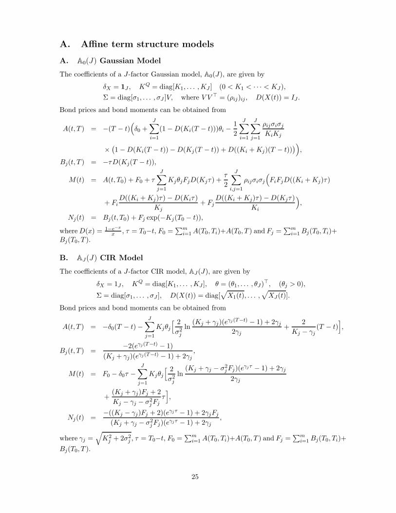
A. Affine term structure models

A. A0(J) Gaussian Model

The coefficients of a J-factor Gaussian model, A0(J), are given by

δX = 1J , KQ = diag[K1, . . . ,KJ ] (0 < K1 < · · · < KJ),

Σ = diag[σ1, . . . , σJ ]V, where V V > = (ρij)ij , D(X(t)) = IJ .

Bond prices and bond moments can be obtained from

A(t, T ) = −(T − t)(

δ0 +

J∑

i=1

(1 − D(Ki(T − t)))θi −1

2

J∑

i=1

J∑

j=1

ρijσiσj

KiKj

×(

1 − D(Ki(T − t)) − D(Kj(T − t)) + D((Ki + Kj)(T − t)))

)

,

Bj(t, T ) = −τD(Kj(T − t)),

M(t) = A(t, T0) + F0 + τ

J∑

j=1

KjθjFjD(Kjτ) +τ

2

J∑

i,j=1

ρijσiσj

(

FiFjD((Ki + Kj)τ)

+ FiD((Ki + Kj)τ) − D(Kiτ)

Kj+ Fj

D((Ki + Kj)τ) − D(Kjτ)

Ki

)

,

Nj(t) = Bj(t, T0) + Fj exp(−Kj(T0 − t)),

where D(x) = 1−e−x

x , τ = T0−t, F0 =∑m

i=1 A(T0, Ti)+A(T0, T ) and Fj =∑m

i=1 Bj(T0, Ti)+Bj(T0, T ).

B. AJ(J) CIR Model

The coefficients of a J-factor CIR model, AJ(J), are given by

δX = 1J , KQ = diag[K1, . . . ,KJ ], θ = (θ1, . . . , θJ)>, (θj > 0),

Σ = diag[σ1, . . . , σJ ], D(X(t)) = diag[√

X1(t), . . . ,√

XJ(t)].

Bond prices and bond moments can be obtained from

A(t, T ) = −δ0(T − t) −J

∑

j=1

Kjθj

[ 2

σ2j

ln(Kj + γj)(e

γj (T−t) − 1) + 2γj

2γj+

2

Kj − γj(T − t)

]

,

Bj(t, T ) =−2(eγj (T−t) − 1)

(Kj + γj)(eγj (T−t) − 1) + 2γj

,

M(t) = F0 − δ0τ −J

∑

j=1

Kjθj

[ 2

σ2j

ln(Kj + γj − σ2

j Fj)(eγjτ − 1) + 2γj

2γj

+(Kj + γj)Fj + 2

Kj − γj − σ2j Fj

τ]

,

Nj(t) =−((Kj − γj)Fj + 2)(eγj τ − 1) + 2γjFj

(Kj + γj − σ2j Fj)(eγjτ − 1) + 2γj

,

where γj =√

K2j + 2σ2

j , τ = T0−t, F0 =∑m

i=1 A(T0, Ti)+A(T0, T ) and Fj =∑m

i=1 Bj(T0, Ti)+

Bj(T0, T ).

25