www.elsevier.com/locate/rgg

Approximation of a near-vertical boundary in the problemsof pulsed electromagnetic soundings

N.V. Shtabel’ a,*, M.I. Epov a,b, E.Yu. Antonov a, M.A. Korsakov a

a A.A. Trofimuk Institute of Petroleum Geology and Geophysics, Siberian Branch of the Russian Academy of Sciences,pr. Akademika Koptyuga 3, Novosibirsk, 630090, Russia

b Novosibirsk State University, ul. Pirogova 2, Novosibirsk, 630090, Russia

Received 19 December 2012; accepted 23 May 2013

Abstract

We analyze the results of a mathematical simulation of pulsed electromagnetic fields in geologic media with dipping near-vertical boundariesas well as interpretations within approximating block models and a layered homogeneous conducting model. We consider the possibilities andlimitations of these approaches to the inversion of data from pulsed soundings of actual geologic media.© 2014, V.S. Sobolev IGM, Siberian Branch of the RAS. Published by Elsevier B.V. All rights reserved.

Keywords: vector finite-element method; 3D modeling; pulsed electromagnetic soundings

Introduction and problem formulation

The theory of nonstationary soundings is based on analysisof the spatial distribution of the electromagnetic field inhorizontally layered models for conducting nonmagnetic iso-tropic geologic media. The most widespread ground unitconsists of several closed circuits (coils): one transmitter andreceivers.

When current within the circuit is switched off, ring eddycurrent develops beneath the surface of the conductinghalf-space, according to Faraday’s induction law. The electro-magnetic field is formed by secondary eddy currents inducedin the conducting parts of the medium.

Eddy currents make up moving toroid structures, oftencalled “smoke rings.” Some time after the switch-off, the eddycurrent toroid dips into the medium and its radius andcross-section increase. In the conducting half-space, the toroidcenter moves along a straight path inclined at ~28° to itssurface (Epov et al., 1994; Nabighian, 1979). If a horizontallylayered model is based on an insulator, its path levels out andit begins to move horizontally with time (so-called S zone).In this case, the electric field does not cross the innerboundaries, at which conductivity changes in a saltatorymanner.

The described process degenerate in terms of the generationof the secondary electromagnetic field, because sources of thesecond type (charges) do not participate therein. They appearin the medium in the presence of nonhorizontal boundaries.The eddy electric field crosses the inner boundaries, on whosesurface charges appear with a density proportional to theaverage normal component of the electric field at the bound-ary. The proportionality coefficient is called “the contrastcoefficient” and described by the simple expression

k12 = σ+ − σ−σ+ + σ−

,

where σ+, σ− are the conductivities of the medium at both

sides of the boundary.Importantly, the surface charges are confined to the

boundaries and can move only along them. On the other hand,the eddy current toroid moves within the entire half-space overtime. In this case, the eddy currents and surface chargesinteract, especially if there are several dipping boundaries inthe medium. The conventional division of the field into twomodes—induction (eddy currents) and galvanic (charges)—loses its physical meaning and cannot be used to the full whenthe behavior of the nonstationary electromagnetic field isanalyzed.

Present-day systems of 3D inversion are usually based ona class of models consisting of a set of conducting areas, whichare separated by a system of horizontal and vertical bounda-

Russian Geology and Geophysics 55 (2014) 89–97

* Corresponding author.E-mail address: nadino2000@mail.ru (N.V. Shtabel’)

Available online at www.sciencedirect.com

ScienceDirect

ed.

+1068-7971/$ - see front matter D 201 IGM, Siberian Branch of the RAS. Published by Elsevier B.V. All rights reservV.S. S bolevo

http://dx.doi.org/10.1016/j.rgg.2013.12.0074,

ries. Such a description of the medium leaves open thequestion of measured-signal inversion in widespread cases,when dipping boundaries are present. How adequate theapproximation of the dipping boundary by a set of horizontaland vertical planes is, remains unclear. If their number is large,it is evident from physical considerations that the values ofnonstationary electromagnetic fields in these two models willapproach one another. If the number of the approximatinghorizontal and vertical plane boundaries is small, the distribu-tion of surface charges at the dipping boundary will differconsiderably. It is continuous at the dipping boundary, and thedensity at the horizontal boundaries will change in a saltatorymanner.

Forward mathematical modeling is used in this study toassess the possibility of describing dipping boundaries bysimpler models with horizontal and vertical boundaries.

For simplicity, we consider a model with one dipping (40º)plane separating two areas of different conductivities. It willbe approximated by a stepwise set of vertical and horizontalsurfaces. The number and sizes of the steps necessary for theapproximation of the dipping boundary will be defined so thatthe nonstationary fields on the surface of the half-space willdiffer by no more than 1–3%. The behavior of the nonstation-ary electromagnetic field will be analyzed in more complicatedmodels with several dipping boundaries. Finally, the conse-quences of model inconsistency in the inversion of suchsignals within horizontally layered models will be considered.

Models for the medium and sounding unit

The model is a parallelepiped measuring 3 × 3 × 4 km anddivided into two subareas: almost nonconducting (air) andconducting (ground), each 2 km high. We presume that themedium is nonmagnetic and nonpolarizing (µ = µ0 = 4π ×107 H/m, ε = ε0 = 8.854 × 10−12 F/m). The air resistivity istaken equal to 106 Ohm⋅m. The sounding unit, located on thesurface of the conducting medium, consists of coaxial squarecoils (transmitter, 100 × 100 m; receiver, 25 × 25 m).

Cartesian coordinates xyz are introduced. Their origincoincides with the center of the transmitter coil. The daysurface is described by the equation z = 0. The inner bounda-ries are tilted with respect to the day surface. The tilt anglesof the boundaries on the vertical plane x0z will be designatedby θ.

Model 1 (Fig 1a). The conducting area is divided by adipping plane crossing the day surface at a distance of 500 mfrom the unit center at θ = 40º. The subarea to the right ofthe dipping boundary has a resistivity of 200 Ohm⋅m, whereasthat to the left, 10 Ohm⋅m.

Models 2 and 3 (Fig. 1b, c) have the same structure butdifferent resistivities. Model 2 has two dipping boundaries.The main boundary 1 is tilted at θ = 40° (as in model 1) andperpendicular to the additional boundary 2. The intersectionof the dipping boundaries in model 3 is localized 500 m todepth from the unit center. The depth of the intersection ofthe dipping planes in model 4 is 100 m. The resistivities of

the subareas to the right and to the left of boundary 1 are 200and 10 Ohm⋅m. The area bounded by the dipping planes inmodels 2 and 3 might be conducting (resistivity 5 Ohm⋅m) ornonconducting (resistivity 1000 Ohm⋅m).

Model 4 (Fig. 1d). The conducting area is divided intolayers by three horizontal boundaries (z = 250, 500, and750 m). The dipping boundary crosses them at θ = 40º. Theupper layer (250 m thick) to the right of the dipping boundaryis characterized by two resistivity values: 5 and 1000 Ohm⋅m.The second layer has a resistivity of 200 Ohm⋅m, and theunderlying layer, 10 Ohm⋅m.

The modeled signal is nonstationary electromotive force(EMF) observed in the receiver coil after switching off thegenerator. Recording time, up to 10 ms.

Mathematical simulation

As the studied model is essentially three-dimensional, thesimulation method should be selected with regard to thedimensions and configuration of the sounding unit as well asthe structure of the area. The method should take into accountthe influence of boundaries with very contrasting conductivi-ties. The above requirements are fulfilled by the vectorfinite-element method (VFEM). Tetrahedral elements are usedin the triangulation, because they permit “condensing” the gridnear the sounding unit (coil–coil) and/or other small elementsof the medium. The solution of the forward problem is theEMF induced in the receiver circuit depending on time afterswitching off the current pulse in the transmitter coil.

The electric field in the quasi-stationary approximation,which appears in the medium after switching off the transmit-ter current, is described by the corollary of Maxwell’sequations

rot µ−1 rot E + σ

∂E∂t

= − ∂J0

∂t,

E × n

∂Ω = 0, E

t = 0

= 0,

(1)

where E is the vector of the electric-field intensity; J0, vectorof the extrinsic-current density in the transmitter vs. time; µ,magnetic permeability; σ, conductivity of the medium; and∂Ω, outer boundaries.

Let us introduce the functional spaces in which the solutionof (1) will be searched for:

H (rot, Ω) = u ∈ L 2(Ω) | ∇ × u ∈ L 2(Ω)

,

H0 (rot, Ω) = u ∈ H (rot, Ω) | u × n

|∂Ω = 0

.

With the corresponding scalar product and norms,

(u, v)Ω = ∫ Ω

u ⋅ v dx, ||u|| = √(u, u)Ω ,

||u||H (rot, Ω)2 = ||u||Ω

2 + ||∇ × u||Ω2 .

90 N.V. Shtabel’ et al. / Russian Geology and Geophysics 55 (2014) 89–97

Let us carry out a variational formulation of the problem:

to find E ∈ H 0 (rot, Ω) × (0, T) for given J ∈ L 2(Ω) × (0, T),so that ∀W ∈ H0 (rot, Ω) × (0, T) is fulfilled

(µ−1 rot E, rot W)Ω + σ ∂E∂t

, W Ω

=

− ∂J∂t

, W Ω

− ∫ Ω

µ−1 (W × n) rot E dS. (2)

The finite-dimensional solution Eh, which satisfies (2), isan expansion in basic functions associated with triangulationelements:

E h (x, t) = ∑ i = 1

N

ei (t) Wi (x), Wi ∈ H h (rot, Ω),

where Wi indicates elements of the discrete subspace

H h (rot, Ω), defined as

H h (rot, Ω) = span W1, W2, ...,Wn

⊂ H0 (rot, Ω).

Since the simulation method is the VFEM, Nédélec’s vectoredge functions of the first order, associated with the edges ofthe tetrahedral division (Nédélec, 1980), are selected to be theWi basic functions. The use of the edge basis permitsautomatic fulfilment of the conditions of the continuity of theelectric-field tangential components at the boundaries directlyin the variational formulation (Nédélec, 1986).

At the outer boundaries of the simulation domain, theelectric-field tangential component is taken equal to zero:

E × n |∂Ω = 0 (Tamm, 1976). The size of the area is determinedfrom the distance between the outer boundary and the unit. Itshould be no less than 15 sizes of the transmitter coil on thehorizontal plane, whereas the EMF attenuation should be noless than 200 dB.

With regard to the expansion and boundary conditions, thediscrete analog of the variational formulation will take thefollowing form:

to find E h ∈ H h (rot, Ω) × (0, T) for J ∈ L 2(Ω) × (0, T), sothat the equation

(µ−1 rot E h, rot W

h)Ω + σ ∂E h

∂t, W h

Ω

= − ∂J∂t

, W h Ω

is fulfilled for ∀Wh ∈ Hh(rot, Ω) × (0, T).In matrix form, it looks like

A e + σ C

∂e∂t

= − ∂F∂t

,

where

[A] ij = ∫ Ω

µ−1 rot Wi ⋅ rot Wj dΩ, i, j = 1, Ne,

[C] ij = ∫ Ω

Wi ⋅ Wj dΩ, i, j = 1, Ne,

[F] i = ∫ Ω

J 0 ⋅ Wi dΩ, i, j = 1, Ne,

Fig. 1. Geometry of the computational domains. a–d, See description in the text. 1–4, boundaries.

N.V. Shtabel’ et al. / Russian Geology and Geophysics 55 (2014) 89–97 91

A program modeling the nonstationary electromagneticfield in an inhomogeneous conducting medium was developedin C++ by the above algorithms (Epov et al., 2012).

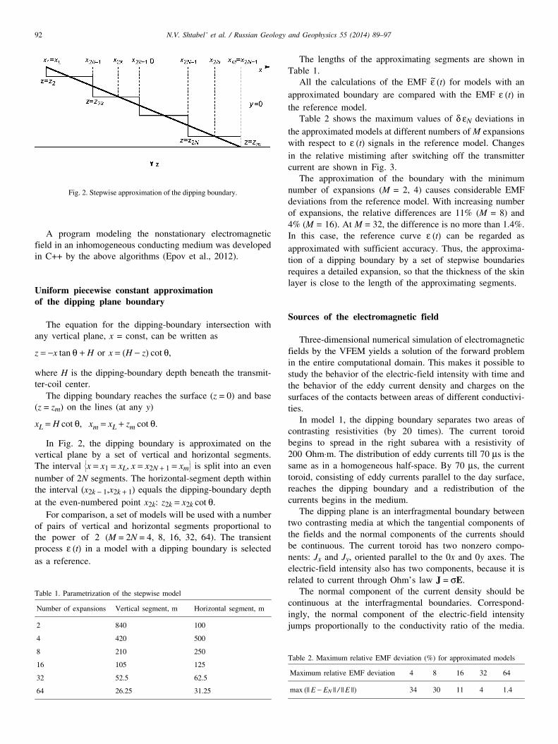
Uniform piecewise constant approximation of the dipping plane boundary

The equation for the dipping-boundary intersection withany vertical plane, x = const, can be written as

z = −x tan θ + H or x = (H − z) cot θ,

where H is the dipping-boundary depth beneath the transmit-ter-coil center.

The dipping boundary reaches the surface (z = 0) and base(z = zm) on the lines (at any y)

xL = H cot θ, xm = xL + zm cot θ.

In Fig. 2, the dipping boundary is approximated on thevertical plane by a set of vertical and horizontal segments.The interval

x = x1 = xL, x = x2N + 1 = xm

is split into an even

number of 2N segments. The horizontal-segment depth withinthe interval (x2k − 1,x2k + 1) equals the dipping-boundary depthat the even-numbered point x2k: z2k = x2k cot θ.

For comparison, a set of models will be used with a numberof pairs of vertical and horizontal segments proportional tothe power of 2 (M = 2N = 4, 8, 16, 32, 64). The transientprocess ε (t) in a model with a dipping boundary is selectedas a reference.

The lengths of the approximating segments are shown inTable 1.

All the calculations of the EMF ε~ (t) for models with anapproximated boundary are compared with the EMF ε (t) inthe reference model.

Table 2 shows the maximum values of δ εN deviations inthe approximated models at different numbers of M expansionswith respect to ε (t) signals in the reference model. Changesin the relative mistiming after switching off the transmittercurrent are shown in Fig. 3.

The approximation of the boundary with the minimumnumber of expansions (M = 2, 4) causes considerable EMFdeviations from the reference model. With increasing numberof expansions, the relative differences are 11% (M = 8) and4% (M = 16). At M = 32, the difference is no more than 1.4%.In this case, the reference curve ε (t) can be regarded asapproximated with sufficient accuracy. Thus, the approxima-tion of a dipping boundary by a set of stepwise boundariesrequires a detailed expansion, so that the thickness of the skinlayer is close to the length of the approximating segments.

Sources of the electromagnetic field

Three-dimensional numerical simulation of electromagneticfields by the VFEM yields a solution of the forward problemin the entire computational domain. This makes it possible tostudy the behavior of the electric-field intensity with time andthe behavior of the eddy current density and charges on thesurfaces of the contacts between areas of different conductivi-ties.

In model 1, the dipping boundary separates two areas ofcontrasting resistivities (by 20 times). The current toroidbegins to spread in the right subarea with a resistivity of200 Ohm⋅m. The distribution of eddy currents till 70 µs is thesame as in a homogeneous half-space. By 70 µs, the currenttoroid, consisting of eddy currents parallel to the day surface,reaches the dipping boundary and a redistribution of thecurrents begins in the medium.

The dipping plane is an interfragmental boundary betweentwo contrasting media at which the tangential components ofthe fields and the normal components of the currents shouldbe continuous. The current toroid has two nonzero compo-nents: Jx and Jy, oriented parallel to the 0x and 0y axes. Theelectric-field intensity also has two components, because it isrelated to current through Ohm’s law J = σE.

The normal component of the current density should becontinuous at the interfragmental boundaries. Correspond-ingly, the normal component of the electric-field intensityjumps proportionally to the conductivity ratio of the media.

Table 1. Parametrization of the stepwise model

Number of expansions Vertical segment, m Horizontal segment, m

2 840 100

4 420 500

8 210 250

16 105 125

32 52.5 62.5

64 26.25 31.25

Table 2. Maximum relative EMF deviation (%) for approximated models

Maximum relative EMF deviation 4 8 16 32 64

max (|| E − EN || / || E ||) 34 30 11 4 1.4

Fig. 2. Stepwise approximation of the dipping boundary.

92 N.V. Shtabel’ et al. / Russian Geology and Geophysics 55 (2014) 89–97

The continuity of the normal current component on theinclined surface is ensured by the surface charges at theboundary, which change the electric-field intensity and theconfiguration of the currents in the medium. Near the dippingboundary, a third component of the electric field Ez appearsunder the effect of induced surface charges, which forms the

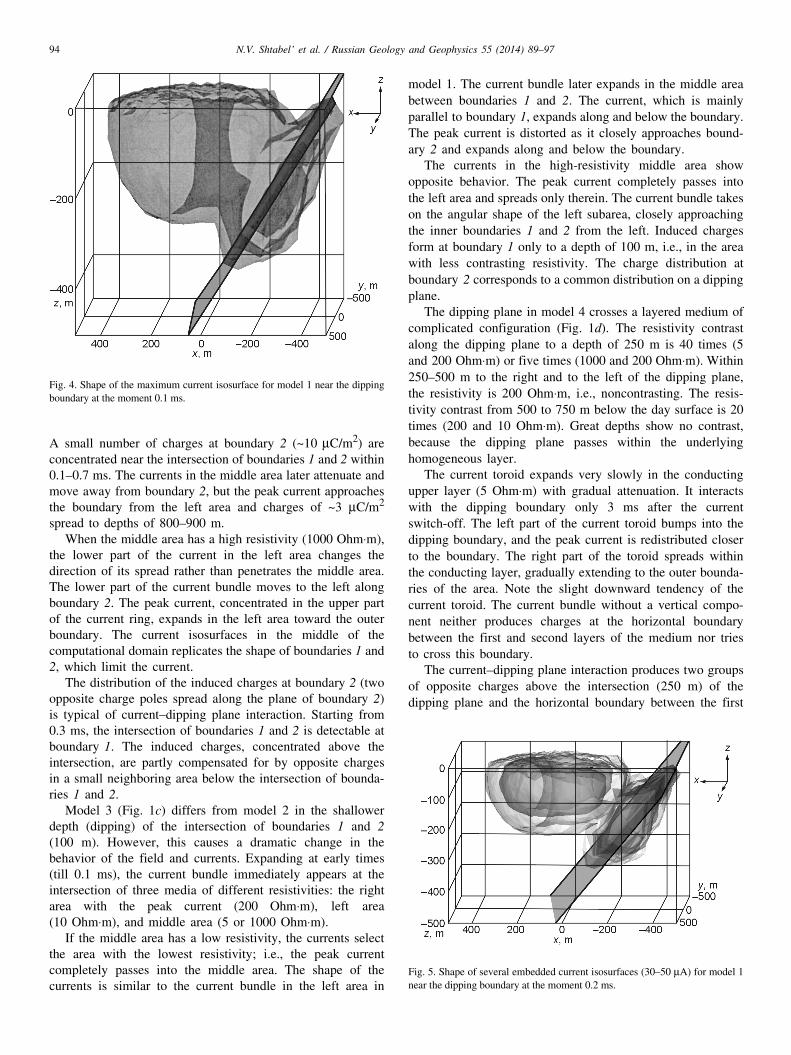
normal field component E n = E × n together with Ex. As the current toroid approaches the boundary, its isosur-

faces change their configuration. In a homogeneous medium,all the current-density isosurfaces are toroids of differentthicknesses with a single center. As the electric field interactswith the dipping plane, the current isosurfaces transform intoa structure combining a toroid and an isosurface localized onthe dipping-surface plane (Fig. 4). Within 0.1–0.2 ms, thecurrent values are redistributed between the toroid and theisosurfaces on the boundary plane (Fig. 5).

By 0.70 ms, the currents in the right subarea (resistivity200 Ohm⋅m) completely cross the boundary into an area witha resistivity of 10 Ohm⋅m, forming a new system of currentsnear the interfragmental boundary. The latter is asymmetricand extends along the inclined plane. The peak currents areconcentrated in the upper part of the current bundle, and theirisosurfaces take on the shape of a crescent with ends down.Isosurfaces with lower values but larger surface area areclosed, and their center is localized at a depth of 350–400 m.The newly formed current bundle of the new configuration

spreads in the left subarea parallel to the dipping plane(Fig. 6).

Model 2 (Fig. 1b) has two dipping boundaries (boundary 1is the same as in model 1). The plane boundary 2 isperpendicular to boundary 1. The subarea to the right ofboundary 1 will be called right. The part of the area limitedby boundaries 1 and 2 will be called middle, and the remainingpart of the medium to the left of boundaries 1 and 2 will becalled left. The resistivity contrast at boundary 2 equals 2(resistivity of the middle area is 5 Ohm⋅m) or 100 (resistivityof the middle area is 100 Ohm⋅m). The resistivity contrast atboundary 1 is 20 to a depth of 500 m and 2 or 100 at depthsgreater than 500 m, depending on the middle-area resistivity.

The current vortex begins to spread in model 2 similarlyto that in model 1, i.e., approaches boundary 1, interacts withit, and changes its configuration during the transition to theleft subarea. The subsequent behavior of the currents dependson the middle-area resistivity. If the middle area has a highconductivity, the currents formed near the upper part ofboundary 1 partly flow into the middle area and spreadtherein, predominantly stretching along boundary 1. In low-resistivity areas (5 Ohm⋅m), the current distribution has a lowvelocity, whereas the current-attenuation rate is high.

The maximum concentration of charges at boundary 1(~2 mC/m2) as the current bundle passes from right to leftsubarea. As the currents pass to the left subarea, the chargestend to attenuate and spread downward on the boundary plane.

Fig. 3. Relative error of the EMF (V) of the form E (t) − E~

(t) / E (t) vs. time (s). E (t), EMF for a model with a dipping boundary; E

~ (t), EMF curves for models

with a boundary approximated by 2N segments. 2N, cipher of the curves.

N.V. Shtabel’ et al. / Russian Geology and Geophysics 55 (2014) 89–97 93

A small number of charges at boundary 2 (~10 µC/m2) areconcentrated near the intersection of boundaries 1 and 2 within0.1–0.7 ms. The currents in the middle area later attenuate andmove away from boundary 2, but the peak current approachesthe boundary from the left area and charges of ~3 µC/m2

spread to depths of 800–900 m.When the middle area has a high resistivity (1000 Ohm⋅m),

the lower part of the current in the left area changes thedirection of its spread rather than penetrates the middle area.The lower part of the current bundle moves to the left alongboundary 2. The peak current, concentrated in the upper partof the current ring, expands in the left area toward the outerboundary. The current isosurfaces in the middle of thecomputational domain replicates the shape of boundaries 1 and2, which limit the current.

The distribution of the induced charges at boundary 2 (twoopposite charge poles spread along the plane of boundary 2)is typical of current–dipping plane interaction. Starting from0.3 ms, the intersection of boundaries 1 and 2 is detectable atboundary 1. The induced charges, concentrated above theintersection, are partly compensated for by opposite chargesin a small neighboring area below the intersection of bounda-ries 1 and 2.

Model 3 (Fig. 1c) differs from model 2 in the shallowerdepth (dipping) of the intersection of boundaries 1 and 2(100 m). However, this causes a dramatic change in thebehavior of the field and currents. Expanding at early times(till 0.1 ms), the current bundle immediately appears at theintersection of three media of different resistivities: the rightarea with the peak current (200 Ohm⋅m), left area(10 Ohm⋅m), and middle area (5 or 1000 Ohm⋅m).

If the middle area has a low resistivity, the currents selectthe area with the lowest resistivity; i.e., the peak currentcompletely passes into the middle area. The shape of thecurrents is similar to the current bundle in the left area in

model 1. The current bundle later expands in the middle areabetween boundaries 1 and 2. The current, which is mainlyparallel to boundary 1, expands along and below the boundary.The peak current is distorted as it closely approaches bound-ary 2 and expands along and below the boundary.

The currents in the high-resistivity middle area showopposite behavior. The peak current completely passes intothe left area and spreads only therein. The current bundle takeson the angular shape of the left subarea, closely approachingthe inner boundaries 1 and 2 from the left. Induced chargesform at boundary 1 only to a depth of 100 m, i.e., in the areawith less contrasting resistivity. The charge distribution atboundary 2 corresponds to a common distribution on a dippingplane.

The dipping plane in model 4 crosses a layered medium ofcomplicated configuration (Fig. 1d). The resistivity contrastalong the dipping plane to a depth of 250 m is 40 times (5and 200 Ohm⋅m) or five times (1000 and 200 Ohm⋅m). Within250–500 m to the right and to the left of the dipping plane,the resistivity is 200 Ohm⋅m, i.e., noncontrasting. The resis-tivity contrast from 500 to 750 m below the day surface is 20times (200 and 10 Ohm⋅m). Great depths show no contrast,because the dipping plane passes within the underlyinghomogeneous layer.

The current toroid expands very slowly in the conductingupper layer (5 Ohm⋅m) with gradual attenuation. It interactswith the dipping boundary only 3 ms after the currentswitch-off. The left part of the current toroid bumps into thedipping boundary, and the peak current is redistributed closerto the boundary. The right part of the toroid spreads withinthe conducting layer, gradually extending to the outer bounda-ries of the area. Note the slight downward tendency of thecurrent toroid. The current bundle without a vertical compo-nent neither produces charges at the horizontal boundarybetween the first and second layers of the medium nor triesto cross this boundary.

The current–dipping plane interaction produces two groupsof opposite charges above the intersection (250 m) of thedipping plane and the horizontal boundary between the first

Fig. 5. Shape of several embedded current isosurfaces (30–50 µA) for model 1near the dipping boundary at the moment 0.2 ms.

Fig. 4. Shape of the maximum current isosurface for model 1 near the dippingboundary at the moment 0.1 ms.

94 N.V. Shtabel’ et al. / Russian Geology and Geophysics 55 (2014) 89–97

and second layers of the medium (Fig. 7). The vertical currentcomponent Jz, which replicates the shape of the inducedcharges, appears in this part of the dipping boundary. Ascompared with model 1, in which the right part of the currenttoroid turned toward the dipping boundary and closed thesystem of currents, the right part of the currents in model 4completely attenuates without leaving the first layer. Thecurrents in the second layer fail to form a closed system overthe modeling period. The isosurfaces of the currents areparaboloids flowing from the dipping plane, whose upper partreplicates the upper boundary of the second layer (combinationof the horizontal boundary and the upper part of the dippingplane). This shape of the currents is due to the predominanceof two current components, Jx and Jz. The current componentJy, tangent to the dipping plane, passes into the second layerand attenuates therein at the penetration depth.

The distribution of the induced charges corresponds to thatof the contrasts along the dipping plane. The induced chargesaccumulate above the intersection of the first horizontalboundary with the dipping plane at a depth of 250 m. At latetimes (more than 13 ms), the intersection of the dipping planewith the second horizontal boundary (500 m) is slightly litfrom the bottom by the induced charges. The value of thecharges is ~0.3 µC/m2.

The current bundle for the high-resistivity first layerspreads fast, so that the left part of the bundle touches thedipping plane already at very early times (20–30 µs). Thecurrent does not manage to attenuate and penetrates farthrough the dipping boundary (~100 m). The shape of thecurrent resembles the left part of the current bundle, which islocated to the left of the boundary and bumps into it. Within0.1–0.3 ms, the currents shift gradually down the dippingplane with simultaneous attenuation of the horizontal part ofthe currents, which replicate the shape of the initial toroid.The subsequent behavior of the currents is similar, but the

absolute values of the current are higher owing to its fastpenetration into the area with a resistivity of 200 Ohm⋅m andit spreads farther within the simulation area.

This is evident from the distribution of the induced charges.The induction is carried out in two parts of the dipping plane:at depths of 0–250 and 500–750 m. The charges are redistrib-uted with time, first to a depth of 250 m, and then chargesappear and spread between the horizons z = –500 m andz = –750 m (Fig. 8).

Inversion of the data obtained in the models with dipping boundaries

Transient EMF curves are mostly interpreted within layeredhomogeneous models with plane-parallel boundaries, becausethese models possess the best developed set of programs andalgorithms for quantitative inversion of the data. As pointedout above, eddy currents serve as signal sources in this case,whereas the part connected with charges does not exist. Asthese sources are important in media with dipping boundaries,inversion within a horizontally layered model will not yield arealistic spatial distribution of resistivities because of consid-erable inconsistency between the model data and the interpre-tation technique.

Transient EMF curves obtained on the profile intersectingthe dipping boundary at a right angle were used as the initialdata (model 1). The inversion was conducted in the TEM-IPsoftware (Antonov and Orlovskaya, 2010; Antonov et al.,2010, 2011; Shein et al., 2012; Shtabel’ and Antonov, 2011).Figure 9 shows a geoelectric section obtained from theinversion of the model data calculated for the profile whichcrosses the areas separated by the dipping boundary. Alongwith considerable resistivity differences detected by 1D inver-

Fig. 6. Shape of several embedded current isosurfaces (0.3–0.5 µA) for model 1at the moment 10 ms.

Fig. 7. Shape of several embedded current isosurfaces (0.3–0.5 µA) for model 4at the moment 5 ms.

N.V. Shtabel’ et al. / Russian Geology and Geophysics 55 (2014) 89–97 95

sion, we get a wrong idea of the localization of the dippingboundary.

Conclusions

The studies show that, if near-vertical boundaries areapproximated by few rectangular blocks (fewer than ten), theerror in EMF curves obtained from the solution of a forwardproblem is too high for these curves to be used in the solutionof an inverse problem. On the other hand, models constructedwith regard to the minimum deviation of EMF curves do notcorrespond to the initial model for the medium. The applica-tion of block structures in models used for solving inverse

problems is justified only with a large number of small blocks.It is incorrect to select a model with blocks whose dimensionsare close to those of the coil and domain, because this selectionyields a model without any common points with the actualsection. The solution of inverse problems should be based onthat of a forward problem in areas with curved boundaries asa 3D problem with regard to all the factors affecting theelectromagnetic field.

The study was supported by the Ministry of Education andScience of the Russian Federation, Agreement no.14.V37.21.0615 “Development and Application of EfficientPrograms and Algorithms for Modeling Nonstationary Elec-tromagnetic Fields in Three-Dimensional Conducting andPolarizing Geologic Media.”

Fig. 8. Distribution of the charges along the dipping plane at the moment 0.63 ms for model 4.

Fig. 9. Geoelectric section from inversion within a model for a horizontally layered medium.

96 N.V. Shtabel’ et al. / Russian Geology and Geophysics 55 (2014) 89–97

References

Antonov, E.Yu., Orlovskaya, N.V., 2010. Numerical simulation of pulsedsoundings of conducting near-vertical inhomogeneities [electronic re-source], in: Int. Sci. Conf. “Electromagnetic Methods-2010” (Irkutsk,15–20 August 2010) [in Russian]. CD-ROM, ISBN 978-5-88942-096-5.

Antonov, E.Yu., Kozhevnikov, N.O., Korsakov, M.A., 2010. TEM-IP—inter-pretation software for transient inductive EM data with respect to inducedpolarization [electronic resource], in: Int. Sci. Conf. “ElectromagneticMethods-2010” (Irkutsk, 15–20 August 2010) [in Russian]. CD-ROM,ISBN 978-5-88942-096-5.

Antonov, E.Yu., Shtabel’, N.V., Korsakov, M.A., 2011. Numerical simulationand inversion of data from pulsed soundings of complicated geologicmedia, in: Erofeev, L.Ya., Isaev, V.I. (Eds.), Geophysical Methods inProspecting [in Russian]. Izd. Tomsk. Politekh. Univ., Tomsk, pp. 8–11.

Epov, M.I., Sukhorukova, K.V., Antonov, E.Yu., 1994. Kinematics of thenonstationary electromagnetic field in layered conducting media, in:Theory and Practice of Magnetotelluric Soundings, Proc. Conf. (Moscow,20–23 December 1994) [in Russian]. Moscow, pp. 11–12.

Epov, M.I., Shurina, E.P., Shtabel, N.V., 2012. Features of 3D electromag-netic fields modeling for geoelectric problems, in: ACE2012—7th Work-shop on Advanced Computational Electromagnetics 29.02.–02.03.2012,

Karlsruhe Inst. of Technology (KIT), Karlsruhe, electronic resource,http://ace2012.math.kit.edu/abstracts/shtabel_epov_shurina.pdf.

Nabighian, M.N., 1979. Quasi-static transient response of a conductinghalf-space: An approximate representation. Geophysics 44 (10), 1700–1705.

Nédélec, J.-C., 1980. Mixed finite elements in R3. Numerische Mathematik35 (3), 315–341.

Nédélec, J.-C., 1986. A new family of mixed finite elements in R3.Numerische Mathematik 50 (1), 57–81.

Shein, A.N., Antonov, E.Yu., Kremer, I.A., Ivanov, M.I., 2012. InterpretationTEM-data by the program Modem3D for 3D modeling of transientelectromagnetic field, in: The 6th Int. Siberian Early Career GeoScientistsConf.: Proc. of the Conf. (Novosibirsk, 9–23 June 2012). IGM and IPPGSB RAS, NSU, Novosibirsk, pp. 303–304.

Shtabel’, N.V., Antonov, E.Yu., 2011. Numerical simulation of the forwardproblem of pulsed soundings in areas with near-vertical inhomogeneities,in: Proc. of the Fifth All-Russ. Workshop, Named after M.N. Berdi-chevskii and L.L. Van’yan, on Electromagnetic Soundings of the Earth—EMS-2011 [in Russian]. Sankt-Peterburgsk. Gos. Univ., St. Petersburg,Book 2, pp. 142–145.

Tamm, I.E., 1976. Fundamentals of the Theory of Electricity: A Handbook,9th ed. [in Russian]. Nauka, Moscow.

Editorial responsibility: A.D. Duchkov

N.V. Shtabel’ et al. / Russian Geology and Geophysics 55 (2014) 89–97 97