APPROXIMATION IN FRACTIONAL SOBOLEV SPACES AND … · APPROXIMATION IN FRACTIONAL SOBOLEV SPACES...
39
HAL Id: hal-01581993 https://hal.archives-ouvertes.fr/hal-01581993 Submitted on 5 Sep 2017 HAL is a multi-disciplinary open access archive for the deposit and dissemination of sci- entific research documents, whether they are pub- lished or not. The documents may come from teaching and research institutions in France or abroad, or from public or private research centers. L’archive ouverte pluridisciplinaire HAL, est destinée au dépôt et à la diffusion de documents scientifiques de niveau recherche, publiés ou non, émanant des établissements d’enseignement et de recherche français ou étrangers, des laboratoires publics ou privés. APPROXIMATION IN FRACTIONAL SOBOLEV SPACES AND HODGE SYSTEMS Pierre Bousquet, Emmanuel Russ, Yi Wang, Po-Lam Yung To cite this version: Pierre Bousquet, Emmanuel Russ, Yi Wang, Po-Lam Yung. APPROXIMATION IN FRACTIONAL SOBOLEV SPACES AND HODGE SYSTEMS. Journal of Functional Analysis, Elsevier, 2019, 276 (5), pp.1430-1478. hal-01581993
Transcript of APPROXIMATION IN FRACTIONAL SOBOLEV SPACES AND … · APPROXIMATION IN FRACTIONAL SOBOLEV SPACES...
HAL Id: hal-01581993https://hal.archives-ouvertes.fr/hal-01581993
Submitted on 5 Sep 2017
HAL is a multi-disciplinary open accessarchive for the deposit and dissemination of sci-entific research documents, whether they are pub-lished or not. The documents may come fromteaching and research institutions in France orabroad, or from public or private research centers.
L’archive ouverte pluridisciplinaire HAL, estdestinée au dépôt et à la diffusion de documentsscientifiques de niveau recherche, publiés ou non,émanant des établissements d’enseignement et derecherche français ou étrangers, des laboratoirespublics ou privés.
APPROXIMATION IN FRACTIONAL SOBOLEVSPACES AND HODGE SYSTEMS
Pierre Bousquet, Emmanuel Russ, Yi Wang, Po-Lam Yung
To cite this version:Pierre Bousquet, Emmanuel Russ, Yi Wang, Po-Lam Yung. APPROXIMATION IN FRACTIONALSOBOLEV SPACES AND HODGE SYSTEMS. Journal of Functional Analysis, Elsevier, 2019, 276(5), pp.1430-1478. �hal-01581993�
APPROXIMATION IN FRACTIONAL SOBOLEV SPACES AND HODGE
SYSTEMS
PIERRE BOUSQUET, EMMANUEL RUSS, YI WANG, PO-LAM YUNG
Abstract. Let d ≥ 2 be an integer, 1 ≤ l ≤ d− 1 and ϕ be a differential l-form on Rd with W 1,d
coefficients. It was proved by Bourgain and Brezis ([5, Theorem 5]) that there exists a differential
l-form ψ on Rd with coefficients in L∞ ∩ W 1,d such that dϕ = dψ. Bourgain and Brezis also askedwhether this result can be extended to differential forms with coefficients in the fractional Sobolevspace W s,p with sp = d. We give a positive answer to this question, in the more general context ofTriebel-Lizorkin spaces, provided that d−κ ≤ l ≤ d−1, where κ is the largest positive integer suchthat κ < min(p, d). The proof relies on an approximation result for functions in W s,p by functions
in W s,p ∩ L∞, even though W s,p does not embed into L∞ in this critical case.
Contents
1 Introduction . . . . . . . . . . . . . . . . . . . . . . . . . . . . . . . . . . . . . . . . . 22 Preliminaries . . . . . . . . . . . . . . . . . . . . . . . . . . . . . . . . . . . . . . . . 7
2.1 The Triebel-Lizorkin spaces . . . . . . . . . . . . . . . . . . . . . . . . . . . . . . 82.2 Inequalities involving the Hardy-Littlewood maximal function . . . . . . . . . . . 9
3 The approximations of f . . . . . . . . . . . . . . . . . . . . . . . . . . . . . . . . . 114 Properties of ωj . . . . . . . . . . . . . . . . . . . . . . . . . . . . . . . . . . . . . . . 14
4.1 Pointwise estimates . . . . . . . . . . . . . . . . . . . . . . . . . . . . . . . . . . . 144.2 Integral estimates . . . . . . . . . . . . . . . . . . . . . . . . . . . . . . . . . . . . 17
5 Estimating h− h . . . . . . . . . . . . . . . . . . . . . . . . . . . . . . . . . . . . . . 205.1 Estimate of
∑r>T . . . . . . . . . . . . . . . . . . . . . . . . . . . . . . . . . . . . 23
5.2 Estimate of∑
r<0 . . . . . . . . . . . . . . . . . . . . . . . . . . . . . . . . . . . . 235.3 Estimate of
∑0≤r≤T . . . . . . . . . . . . . . . . . . . . . . . . . . . . . . . . . . 24
5.4 Conclusion . . . . . . . . . . . . . . . . . . . . . . . . . . . . . . . . . . . . . . . . 256 Estimating g − g . . . . . . . . . . . . . . . . . . . . . . . . . . . . . . . . . . . . . . 25
6.1 Estimate of∑
r≥aαt . . . . . . . . . . . . . . . . . . . . . . . . . . . . . . . . . . . 27
6.2 Estimate of∑
r≤0 . . . . . . . . . . . . . . . . . . . . . . . . . . . . . . . . . . . . 28
6.3 Estimate of∑
0≤r≤aαt . . . . . . . . . . . . . . . . . . . . . . . . . . . . . . . . . . 296.4 Conclusion . . . . . . . . . . . . . . . . . . . . . . . . . . . . . . . . . . . . . . . . 30
7 Completion of the proof of Proposition 3.3 . . . . . . . . . . . . . . . . . . . . . 308 Solving Hodge systems . . . . . . . . . . . . . . . . . . . . . . . . . . . . . . . . . . 319 Appendix: some properties of Schwartz functions . . . . . . . . . . . . . . . . . 3210 Appendix: proof of Proposition 4.8 . . . . . . . . . . . . . . . . . . . . . . . . . 33References . . . . . . . . . . . . . . . . . . . . . . . . . . . . . . . . . . . . . . . . . . . . 36
Date: September 5, 2017.
1

2 PIERRE BOUSQUET, EMMANUEL RUSS, YI WANG, PO-LAM YUNG
1. Introduction
For k ∈ N and 1 < p < ∞, let W k,p(Rd) be the homogeneous Sobolev space on Rd, that is the
completion of C∞c (Rd) under the norm ‖∂kf‖Lp(Rd). It is well-known that while W k,p(Rd) embeds
continuously into Lkp/(d−kp)(Rd) when kp < d, the embedding fails when kp = d. In a ground-breaking paper [5] (see also [4]), Bourgain and Brezis found a remedy for this failure when k = 1
and p = d. They showed that for any f ∈ W 1,d(Rd) and any δ > 0, there exists F ∈ W 1,d∩L∞(Rd)and a constant Cδ > 0 independent of f , such that
(1.1)d−1∑i=1
‖∂i(f − F )‖Ld ≤ δ‖f‖W 1,d ,
and
(1.2) ‖F‖L∞ + ‖F‖W 1,d ≤ Cδ‖f‖W 1,d .
The failure of the embedding of W 1,d(Rd) into L∞(Rd) makes this result rather non-trivial. Theyalso derived many important consequences of this approximation theorem. Among them, theyproved that if l ∈ J1, d − 1K and ϕ is a differential l-form on Rd with W 1,d coefficients, then there
exists a differential l-form ψ on Rd with W 1,d ∩ L∞ coefficients such that
dψ = dϕ.
In this paper, we give an extension of these results to a range of critical Triebel-Lizorkin spacesFα,pq (Rd) that barely fail to embed into L∞. In particular, our results cover the higher order Sobolev
spaces W k,d/k(Rd) where k is an integer with 1 < k < d, and the Sobolev spaces Wα,d/α(Rd) offractional order α ∈ (0, 1), giving an answer to the Open Problem 2 in [5].
Our main result can be stated as follows:
Theorem 1.1. Let α > 0 and p, q ∈ (1,∞) such that αp = d. Let κ be the largest positive integerthat satisfies κ < min{p, d}. Then, for every δ > 0, there exists a constant Cδ > 0 such that, for
every f ∈ Fα,pq (Rd), there exist F ∈ Fα,pq ∩ L∞(Rd) such thatκ∑i=1
‖∂i(f − F )‖Fα−1,pq
≤ δ‖f‖Fα,pq,
and‖F‖L∞ + ‖F‖Fα,pq
≤ Cδ‖f‖Fα,pq.
From Theorem 1.1, we derive:
Theorem 1.2. Let α > 0, p, q ∈ (1,∞) such that αp = d and l ∈ Jd − κ, d − 1K, where κ
is the largest positive integer such that κ < min(p, d). Let ϕ ∈ Fα,pq (ΛlRd). There exists ψ ∈Fα,pq (ΛlRd) ∩ L∞(ΛlRd) such that
dψ = dϕ
and‖ψ‖L∞(ΛlRd) + ‖ψ‖Fα,pq (ΛlRd) . ‖dϕ‖Fα−1,p
q (ΛlRd).
By Fα,pq (ΛlRd), we mean the space of differential l-forms on Rd, the coefficients of which belong
to Fα,pq (Rd) (see Definition 2.1 below). The above statement extends the main result in [6] whichwas restricted to the conditions κ = 1 (which amounts to solving the equation div X = f with

APPROXIMATION IN FRACTIONAL SOBOLEV SPACES AND HODGE SYSTEMS 3
f ∈ Fα,pq ), α > 1/2 and p ≥ q ≥ 2; see also the earlier papers by Maz’ya [16] and also Mironescu[18] when κ = 1, and p = q = 2.
If we do not require the solution ψ in Theorem 1.2 to be in Fα,pq , then the theorem can bededuced from Proposition 2.1 of Van Schaftingen [30], which has a very elegant and simple proof.This elementary approach introduced in [27, 26] has been exploited in various settings, see inparticular Lanzani and Stein [15] and Mitrea and Mitrea [19]. Up to our knowledge however, even
in the framework of Sobolev spaces W 1,d, there is no simple argument to prove the existence of asolution ψ which is both in L∞ and in W 1,d. In the case of the equation divX = f with f ∈ Ld,an algorithmic construction of a solution X ∈ L∞ was proposed in [24].
Many extensions, applications and recent developments of the original results established byBourgain and Brezis in [5, 4] are presented in the excellent overview by Van Schaftingen [32]. Weonly quote some of them here:
(1) more general (higher order) operators than the exterior derivative have been studied in VanSchaftingen [28, 29, 31],
(2) similar problems have been considered when the space Rd is replaced by more generaldomains: half-spaces in Amrouche and Nguyen [1], smooth domains with specific boundaryconditions in Brezis and Van Schaftingen [8], homogeneous groups in Chanillo and VanSchaftingen [9], Wang and Yung [33], symmetric spaces in Chanillo, Van Schaftingen andYung [12, 11], and CR manifolds in Yung [34].
(3) related Hardy inequalities were established by Maz’ya [17] (see also [7]),(4) further applications of this theory can be found in Chanillo and Yung [13] and in Chanillo,
Van Schaftingen and Yung [10].
Let us first briefly recall the strategy of Bourgain and Brezis in their proof of the approximationtheorem of W 1,d(Rd) (that is, (1.1) and (1.2) above), before we turn to the difficulties we must face
in proving Theorem 1.1. First they observe that for f ∈ W 1,d(Rd), the Littlewood-Paley projections∆jf are uniformly bounded in Rd for all j, by Bernstein’s inequality:
‖∆jf‖L∞(Rd) ≤ C‖∇f‖Ld(Rd).
By normalizing f , one may thus assume that ‖∆jf‖L∞(Rd) ≤ 1 for all j ∈ Z. As a result, to
approximate f =∑
j∈Z ∆jf =∑
j∈Z ∆jf · 1 by a bounded function F , one is tempted to set
F (x) =∑j∈Z
∆jf(x)∏j′>j
(1− |∆j′f(x)|),
which would be automatically bounded by a partition of unity identity (see Lemma 3.2 below). Ofcourse this cannot work, for this construction does not distinguish between the “good” directions∂1, . . . , ∂d−1 from the “bad” direction ∂d (whereas (1.1) distinguishes those). Thus Bourgain andBrezis introduce an auxiliary function ωj(x), which controls ∆jf(x) in the sense that
|∆jf | ≤ ωj ≤ ‖∆jf‖L∞(Rd),
while satisfying good derivative bounds such as
|∂iωj | ≤ C2j−σωj for i = 1, . . . , d− 1, and |∂dωj | ≤ C2jωj ;
here σ > 0 is a large parameter only depending on δ. These ωj ’s are constructed in [5] by using a sup-convolution (where one takes a supremum instead of an integral in the definition of a convolution),
4 PIERRE BOUSQUET, EMMANUEL RUSS, YI WANG, PO-LAM YUNG
namely:
ωj(x) = supy∈Rd
|∆jf(y)|e−2j |xd−yd|−2j−σ |x′−y′|,
where x′ − y′ = (x1 − y1, ..., xd−1 − yd−1). With this in hand, one may be tempted to define theapproximating function F by setting
F (x) =∑j∈Z
∆jf(x)∏j′>j
(1− ωj(x)),
which again would be automatically bounded by a partition of unity identity, and which has abetter chance of obeying estimate (1.1). It turns out that this is still not sufficient; indeed, if Fwere such defined, then
f − F =∑j
ωjµj
for some functions µj given by
µj(x) =∑j′<j
∆j′f(x)∏
j′<j′′<j
(1− ωj′′(x)).
These µj ’s are pointwisely bounded by 1 under our normalization of f . Thus to give an upper
bound for ‖∂i(f − F )‖Ld , one term to be controlled is the Ld-norm of∑
j µj∂iωj . But
(1.3)
∥∥∥∥∥∥∑j
|∂iωj ||µj |
∥∥∥∥∥∥Ld
≤ C
∥∥∥∥∥∥∑j
2jωj
∥∥∥∥∥∥Ld
;
it is therefore hopeless to conclude this way, since the right-hand side of (1.3) is even bigger than∥∥∥∥2j |∆jf |∥∥`1
∥∥Ld,
while one can only afford a bound by∥∥∥∥2j∆jf
∥∥`2
∥∥Ld' ‖∇f‖Ld . Bourgain and Brezis have a clever
way out: if instead of∥∥∥∑j 2jωj
∥∥∥Ld
we only needed to estimate∥∥∥∥∥∥∑j
2jωjχAj
∥∥∥∥∥∥Ld
where Aj is the set defined by Aj := {x ∈ Rd : ωj(x) >∑
t>0 2−tωj−t(x)} and χAj is the char-acteristic function of the set Aj , then we would be in good shape because we have a pointwisebound
(1.4)∑j
2jωjχAj ≤ 2 supj
2jωj ,
and the crucial estimate:
(1.5)
∥∥∥∥∥supj∈Z
(2jωj)
∥∥∥∥∥Lp(Rd)
≤ C2σ(d−1)
p ‖∇f‖Lp(Rd)
for any 1 < p <∞. Thus they decompose
∆jf(x) = ∆jf(x)χAcj (x) + ∆jf(x)χAj (x) := gj(x) + hj(x)

APPROXIMATION IN FRACTIONAL SOBOLEV SPACES AND HODGE SYSTEMS 5
so that f =∑
j∈Z gj+∑
j∈Z hj . They then proceed to approximate g :=∑
j∈Z gj and h :=∑
j∈Z hjby
g :=∑j∈Z
gj∏j′>j
(1−Gj′) and h :=∑j∈Z
hj∏j′>j
(1− Uj′)
respectively, where Gj and Uj are some suitable controlling functions that satisfy pointwisely gj ≤Gj ≤ 1 and hj ≤ Uj ≤ 1 (so that g and h are automatically bounded), whereas Gj and Uj are
constructed from the ωj ’s, so that the Ld-norms of ∂i(g − g) and ∂i(h− h) satisfy good estimates
for i = 1, . . . , d − 1. Indeed, in [5], h − h is written as a sum of products, which in turn allows
a direct estimate of ∂i(h − h) by the Leibniz rule; the heuristics centered around equations (1.4)
and (1.5) suggest that ‖∂i(h − h)‖Ld may be small. On the other hand, ∂i(g − g) is estimatedusing Littlewood-Paley inequalities, since it is a sum of pieces that are well-localized in frequency:indeed, note that
(1.6) |∆jf(x)|χAcj (x) ≤∑t>0
2−tωj−t(x),
and while a derivative on the left hand side of (1.6) heuristically gains only 2j , a derivative on eachterm on the right hand side of (1.6) gains 2j−t, which is better when t is large. It is this interplaythat allows them to conclude with the estimate for ∂i(g− g), and hence the proof of their theorem.
Now that we have recalled this basic strategy, we can address the difficulties we faced in extendingthe result of Bourgain and Brezis for W 1,d(Rd), to the full Theorem 1.1 for Fα,pq (Rd). The firstdifficulty arises when α > 1: if we define the controlling functions ωj as in [5] by using a sup-convolution, then the ωj are at best Lipschitz, and in general may not be differentiated more than
once. But an approximation theorem for Fα,pq (Rd) naturally involves taking α derivatives, so asup-convolution construction for the ωj ’s cannot be expected to work when α > 1. Following [33],where Bourgain and Brezis’ result was extended to subelliptic settings, we overcome this by takinga discrete `p convolution instead; morally speaking, this means that we take
(1.7) ωj(x) =
∑r∈2−jZd
(|∆jf |(r)e−2j |x′′−r′′|−2j−σ |x′−r′|
)p1/p
(here r′ and r′′ are the first κ and the last d− κ variables of r respectively, where κ is defined as inTheorem 1.1; similarly for x′ and x′′). For some technical reasons, this is not the precise definitionof ωj we will use; see (3.3) in Section 3 below for the precise construction of ωj . Once the correctdefinition of ωj is in place, roughly speaking we would consider the sets
Aj := {x ∈ Rd : ωj(x) >∑t>0
2−αtωj−t(x)}
(note the dependence of this set on α), and split
∆jf(x) = ∆jf(x)χAcj (x) + ∆jf(x)χAj (x) := gj(x) + hj(x)
as above (actually we would use a smooth version of χAj instead of the sharp cut-off given bythe characteristic function of Aj). We would then proceed as in [5] to approximate
∑j∈Z hj and∑
j∈Z gj , except that several further difficulties must be overcome.
One of them is the proof of the analog of (1.5) in the case q > p. This arises, for instance, when we
prove an approximation theorem for W k,d/k(Rd) with d/2 < k < d (in which case q = 2 > d/k = p).

6 PIERRE BOUSQUET, EMMANUEL RUSS, YI WANG, PO-LAM YUNG
In general, to prove Theorem 1.1 for Fα,pq (Rd), we would like to prove an inequality of the form
(1.8)
∥∥∥∥∥supj∈Z
(2αjωj)
∥∥∥∥∥Lp(Rd)
. 2σκp ‖f‖Fα,pq (Rd).
If ωj was defined as in the putative definition (1.7), then morally speaking, the above inequalitywould admit an easy proof when q ≤ p: indeed, heuristically we have
ωj(x) '
∑r∈Zd
(|∆jf |(x− 2−jr)e−|r
′′|−2−σ |r′|)p1/p
,
so ∥∥∥∥∥supj∈Z
(2αjωj)
∥∥∥∥∥p
Lp(Rd)
=
∫Rd
supj∈Z
(2αjωj(x))pdx
≤∑j∈Z
∫Rd
(2αjωj(x))pdx
=∑j∈Z
∑r∈Zd
(e−|r′′|−2−σ |r′|)p(2αj)p
∫Rd|∆jf(x− 2−jr)|pdx.
The last integral is equal to∫Rd |∆jf |(x)pdx, and
∑r∈Zd(e
−|r′′|−2−σ |r′|)p . 2σκ. Thus∥∥∥∥∥supj∈Z
(2αjωj)
∥∥∥∥∥p
Lp(Rd)
. 2σκ∫Rd
∑j∈Z
(2αj |∆jf(x)|)pdx
. 2σκ∫Rd
∑j∈Z
(2αj |∆jf(x)|)qp/q
dx
where in the last line we have used the embedding `q ↪→ `p if q ≤ p. This would prove (1.8)when q ≤ p, under the putative definition (1.7) of ωj . Unfortunately this simple argument isinsufficient in handling the case when q > p. We found a way out using a logarithmic bound forsome vector-valued ‘shifted’ maximal functions (see Corollary 10.3), which we prove using an oldargument going back to Zo ([35]). We then get a slightly weaker bound than (1.8), one that is offby a logarithmic factor (see Proposition 4.7), but that is still sufficient for our purpose.
A second difficulty arises when α is not an integer or when q 6= 2. Recall that in one step,Bourgain and Brezis estimated ∂i(h − h) in Ld(Rd) by writing it as a sum of products, and then
using the ordinary Leibniz rule. In our case, we need to estimate ∂i(h − h) in Fα−1,pq (Rd), which
is defined only via Littlewood-Paley projections when α is not an integer, or when q 6= 2. Thus wemust know how to estimate the derivative of a sum of products within the realm of Littlewood-Paley theory. If it were not for the sum involved, we could just apply the fractional Leibniz rulefor the space Fα−1,p
q (Rd). But since the sum is present, we found it easier to proceed directly,without resorting to the fractional Leibniz rule. It may also be worth noting here that we runinto an additional difficulty, in the case 0 < α < 1: we find it necessary then to exploit someadditional cancellations offered by the Littlewood-Paley projections ∆j ’s, when we deal with certain
APPROXIMATION IN FRACTIONAL SOBOLEV SPACES AND HODGE SYSTEMS 7
high frequency components of h − h (see the introduction of the parameter T in Section 5 when0 < α < 1).
A final difficulty arises when α ∈ (0, 1/2]. In this case, α is rather small, so the set Acj , given
by Acj = {x ∈ Rd : ωj(x) ≤∑
t>0 2−αtωj−t(x)}, is relatively large. As a result, gj := ∆jf · χAcj is
relatively large, and one expects it to be relatively harder to estimate ∂i(g− g) in Fα−1,pq (Rd). This
is manifested in our need to introduce a parameter aα in Section 6 (see Proposition 6.1), which issmaller than 1 when α ∈ (0, 1/2].Let us end up this introduction with three open problems:
Open problem 1.3. The condition κ < min(p, d) in the statements of Theorems 1.1 and 1.2may not be necessary in general. In [17], Maz’ya proves that for every vector function X ∈Fd/2,22 (Rd;Rd), there exists Y ∈ (F
d/2,22 ∩ L∞)(Rd;Rd) and a scalar function u ∈ F
1+d/2,22 (Rd)
such that
X = Y +∇u.
This coincides with the statement of Theorem 1.2 when p = q = 2, α = d/2 and l = 1, exceptthat this set of parameters is not covered by our assumptions when d ≥ 3. Indeed, the conditionl ∈ Jd− κ, d− 1K cannot be satisfied in that case: this would require κ = d− 1, which is impossiblein view of the conditions κ < p = 2 and d ≥ 3. Is it true that Theorems 1.1 and 1.2 remain truewhen the condition κ < min{p, d} is replaced by κ < d ?
Open problem 1.4. In [33], the conclusion of [5] is extended to a subelliptic context, namely thecase of the Heisenberg groups endowed with a subelliptic Laplacian. The extension of Theorems 1.1and 1.2 to the case of the Heisenberg group is an open problem.
Open problem 1.5. It is likely that Theorem 1.2 can be extended to the case of smooth boundeddomains in Rd, in the spirit of [6].
The paper is organized as follows. After gathering instrumental facts about Triebel-Lizorkin spacesand maximal functions in Section 2, we describe the approximating function F in Theorem 1.1 inSection 3. Section 4 is devoted to proving key estimates for the ωj ’s, which are then used to derive
bounds for h− h (resp. g− g) in Section 5 (resp. Section 6). The proof of Theorem 1.1 is completedin Section 7, while Theorem 1.2 is established in Section 8.
Throughout the paper, if two quantities A(f) and B(f) depend on a function f ranging oversome space L, the notation A(f) . B(f) means that there exists C > 0 such that A(f) ≤ CB(f)for all f ∈ L, while A(f) ' B(f) means that A(f) . B(f) . A(f). The Euclidean ball centered at0 with radius r will be denoted Br.Acknowledgment. Wang was partially supported by NSF Grant No. DMS-1612015. Yung waspartially supported by the Early Career Grant CUHK24300915 from the Hong Kong ResearchGrant Council.
2. Preliminaries
For a brief overview on homogeneous Triebel-Lizorkin spaces, we refer to [25, Chapter 5], [3] andalso [21, Chapter 2].
8 PIERRE BOUSQUET, EMMANUEL RUSS, YI WANG, PO-LAM YUNG
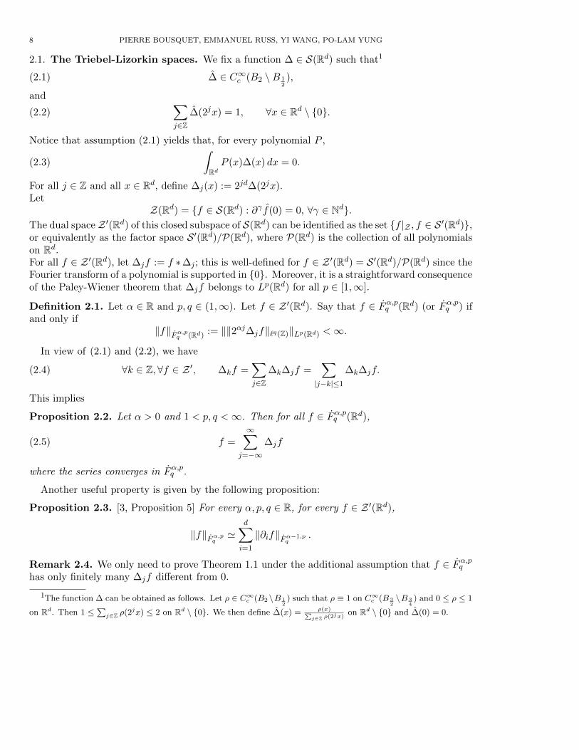
2.1. The Triebel-Lizorkin spaces. We fix a function ∆ ∈ S(Rd) such that1
(2.1) ∆ ∈ C∞c (B2 \B 12),
and
(2.2)∑j∈Z
∆(2jx) = 1, ∀x ∈ Rd \ {0}.
Notice that assumption (2.1) yields that, for every polynomial P ,
(2.3)
∫RdP (x)∆(x) dx = 0.
For all j ∈ Z and all x ∈ Rd, define ∆j(x) := 2jd∆(2jx).Let
Z(Rd) = {f ∈ S(Rd) : ∂γ f(0) = 0, ∀γ ∈ Nd}.The dual space Z ′(Rd) of this closed subspace of S(Rd) can be identified as the set {f |Z , f ∈ S ′(Rd)},or equivalently as the factor space S ′(Rd)/P(Rd), where P(Rd) is the collection of all polynomialson Rd.For all f ∈ Z ′(Rd), let ∆jf := f ∗∆j ; this is well-defined for f ∈ Z ′(Rd) = S ′(Rd)/P(Rd) since theFourier transform of a polynomial is supported in {0}. Moreover, it is a straightforward consequenceof the Paley-Wiener theorem that ∆jf belongs to Lp(Rd) for all p ∈ [1,∞].
Definition 2.1. Let α ∈ R and p, q ∈ (1,∞). Let f ∈ Z ′(Rd). Say that f ∈ Fα,pq (Rd) (or Fα,pq ) ifand only if
‖f‖Fα,pq (Rd) := ‖‖2αj∆jf‖`q(Z)‖Lp(Rd) <∞.
In view of (2.1) and (2.2), we have
(2.4) ∀k ∈ Z,∀f ∈ Z ′, ∆kf =∑j∈Z
∆k∆jf =∑|j−k|≤1
∆k∆jf.
This implies
Proposition 2.2. Let α > 0 and 1 < p, q <∞. Then for all f ∈ Fα,pq (Rd),
(2.5) f =
∞∑j=−∞
∆jf
where the series converges in Fα,pq .
Another useful property is given by the following proposition:
Proposition 2.3. [3, Proposition 5] For every α, p, q ∈ R, for every f ∈ Z ′(Rd),
‖f‖Fα,pq'
d∑i=1
‖∂if‖Fα−1,pq
.
Remark 2.4. We only need to prove Theorem 1.1 under the additional assumption that f ∈ Fα,pq
has only finitely many ∆jf different from 0.
1The function ∆ can be obtained as follows. Let ρ ∈ C∞c (B2 \B 12) such that ρ ≡ 1 on C∞c (B 3
2\B 3
4) and 0 ≤ ρ ≤ 1
on Rd. Then 1 ≤∑j∈Z ρ(2jx) ≤ 2 on Rd \ {0}. We then define ∆(x) = ρ(x)∑
j∈Z ρ(2jx)
on Rd \ {0} and ∆(0) = 0.
APPROXIMATION IN FRACTIONAL SOBOLEV SPACES AND HODGE SYSTEMS 9
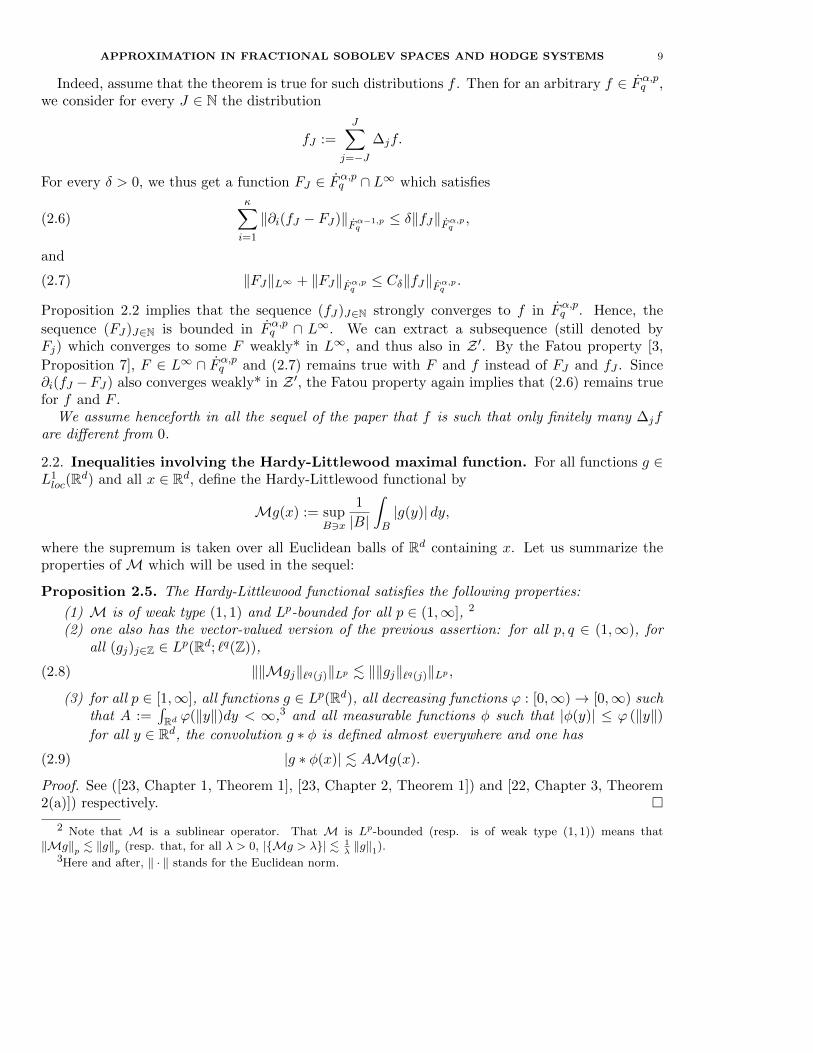
Indeed, assume that the theorem is true for such distributions f . Then for an arbitrary f ∈ Fα,pq ,we consider for every J ∈ N the distribution
fJ :=J∑
j=−J∆jf.
For every δ > 0, we thus get a function FJ ∈ Fα,pq ∩ L∞ which satisfies
(2.6)
κ∑i=1
‖∂i(fJ − FJ)‖Fα−1,pq
≤ δ‖fJ‖Fα,pq,
and
(2.7) ‖FJ‖L∞ + ‖FJ‖Fα,pq≤ Cδ‖fJ‖Fα,pq
.
Proposition 2.2 implies that the sequence (fJ)J∈N strongly converges to f in Fα,pq . Hence, the
sequence (FJ)J∈N is bounded in Fα,pq ∩ L∞. We can extract a subsequence (still denoted byFj) which converges to some F weakly* in L∞, and thus also in Z ′. By the Fatou property [3,
Proposition 7], F ∈ L∞ ∩ Fα,pq and (2.7) remains true with F and f instead of FJ and fJ . Since∂i(fJ −FJ) also converges weakly* in Z ′, the Fatou property again implies that (2.6) remains truefor f and F .
We assume henceforth in all the sequel of the paper that f is such that only finitely many ∆jfare different from 0.
2.2. Inequalities involving the Hardy-Littlewood maximal function. For all functions g ∈L1loc(Rd) and all x ∈ Rd, define the Hardy-Littlewood functional by
Mg(x) := supB3x
1
|B|
∫B|g(y)| dy,
where the supremum is taken over all Euclidean balls of Rd containing x. Let us summarize theproperties of M which will be used in the sequel:
Proposition 2.5. The Hardy-Littlewood functional satisfies the following properties:
(1) M is of weak type (1, 1) and Lp-bounded for all p ∈ (1,∞], 2
(2) one also has the vector-valued version of the previous assertion: for all p, q ∈ (1,∞), forall (gj)j∈Z ∈ Lp(Rd; `q(Z)),
(2.8) ‖‖Mgj‖`q(j)‖Lp . ‖‖gj‖`q(j)‖Lp ,
(3) for all p ∈ [1,∞], all functions g ∈ Lp(Rd), all decreasing functions ϕ : [0,∞)→ [0,∞) suchthat A :=
∫Rd ϕ(‖y‖)dy < ∞,3 and all measurable functions φ such that |φ(y)| ≤ ϕ (‖y‖)
for all y ∈ Rd, the convolution g ∗ φ is defined almost everywhere and one has
(2.9) |g ∗ φ(x)| . AMg(x).
Proof. See ([23, Chapter 1, Theorem 1], [23, Chapter 2, Theorem 1]) and [22, Chapter 3, Theorem2(a)]) respectively. �
2 Note that M is a sublinear operator. That M is Lp-bounded (resp. is of weak type (1, 1)) means that‖Mg‖p . ‖g‖p (resp. that, for all λ > 0, |{Mg > λ}| . 1
λ‖g‖1).
3Here and after, ‖ · ‖ stands for the Euclidean norm.
10 PIERRE BOUSQUET, EMMANUEL RUSS, YI WANG, PO-LAM YUNG
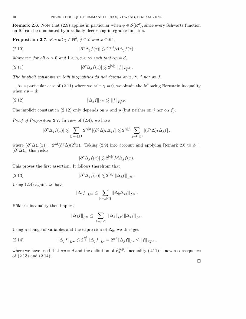
Remark 2.6. Note that (2.9) applies in particular when φ ∈ S(Rd), since every Schwartz functionon Rd can be dominated by a radially decreasing integrable function.
Proposition 2.7. For all γ ∈ Nd, j ∈ Z and x ∈ Rd,
(2.10) |∂γ∆jf(x)| . 2|γ|jM∆jf(x).
Moreover, for all α > 0 and 1 < p, q <∞ such that αp = d,
(2.11) |∂γ∆jf(x)| . 2|γ|j ‖f‖Fα,pq.
The implicit constants in both inequalities do not depend on x, γ, j nor on f .
As a particular case of (2.11) where we take γ = 0, we obtain the following Bernstein inequalitywhen αp = d:
(2.12) ‖∆jf‖L∞ . ‖f‖Fα,pq.
The implicit constant in (2.12) only depends on α and p (but neither on j nor on f).
Proof of Proposition 2.7. In view of (2.4), we have
|∂γ∆jf(x)| .∑|j−k|≤1
2|γ|k |(∂γ∆)k∆jf | . 2|γ|j∑|j−k|≤1
|(∂γ∆)k∆jf | ,
where (∂γ∆)k(x) = 2kd(∂γ∆)(2kx). Taking (2.9) into account and applying Remark 2.6 to φ =(∂γ∆)k, this yields
|∂γ∆jf(x)| . 2|γ|jM∆jf(x).
This proves the first assertion. It follows therefrom that
(2.13) |∂γ∆jf(x)| . 2|γ|j ‖∆jf‖L∞ .
Using (2.4) again, we have
‖∆jf‖L∞ ≤∑|j−k|≤1
‖∆k∆jf‖L∞ .
Holder’s inequality then implies
‖∆jf‖L∞ ≤∑|k−j|≤1
‖∆k‖Lp′ ‖∆jf‖Lp .
Using a change of variables and the expression of ∆k, we thus get
(2.14) ‖∆jf‖L∞ . 2jdp ‖∆jf‖Lp = 2αj ‖∆jf‖Lp ≤ ‖f‖Fα,pq
,
where we have used that αp = d and the definition of Fα,pq . Inequality (2.11) is now a consequenceof (2.13) and (2.14).
�

APPROXIMATION IN FRACTIONAL SOBOLEV SPACES AND HODGE SYSTEMS 11
3. The approximations of f
The present section is devoted to the definition of the function F in Theorem 1.1. Let α > 0and p > 1 such that αp = d. Let f ∈ Fα,pq (Rd), δ > 0 and σ be a large positive integer to be chosen(only depending on δ). For x = (x1, . . . , xd), we define xσ := (2−σx1, . . . , 2
−σxκ, xκ+1, . . . , xd). Theparameter σ discriminates the good directions x1, . . . , xκ from the other ones. In particular, whenone differentiates a function of the form x 7→ u(xσ) along a good direction, an additional factor2−σ arises.Let E be the Schwartz function defined by
(3.1) E(x) := e−(1+‖xσ‖2)12 .
For all j ∈ Z and all x ∈ Rd, let Ej(x) := 2jdE(2jx).Define also
(3.2) T (x) := min(
1, ‖x‖−(d+1))
and
Tj(x) := 2jdT (2jx)
for all j ∈ Z and all x ∈ Rd.We introduce an auxiliary function which can be seen as a substitute of |∆jf |, j ∈ Z:
(3.3) ωj(x) :=
∑r∈Zd
[Tj |∆jf |(2−jr)E(2jx− r)
]p 1p
, x ∈ Rd.
Here and in the sequel, we use the notation Tj |∆jf | for the convolution Tj ∗ |∆jf |. We will provethat ωj inherits the L∞ bounds of |∆jf |. More precisely,
‖∆jf‖L∞ . ‖ωj‖L∞ . 2κσ‖∆jf‖L∞ .
In contrast to |∆jf |, ωj is smooth, as a discrete `p convolution. Moreover, it behaves differently withrespect to good and bad coordinates. This allows to obtain improved estimates on its derivativesalong good directions.
Remark 3.1. Notice that, if, for some x ∈ Rd and some j ∈ Z, ωj(x) = 0, then the definition ofωj yields that Tj |∆jf | (2−jr) = 0 for all r ∈ Z. Since Tj is positive everywhere, it follows that ∆jf
has to vanish on all Rd, which entails that ωj(y) = 0 for all y ∈ Rd.
Let R >> σ be another positive integer to be chosen. Let us consider a smooth function ζjapproximating the characteristic function of the setx ∈ Rd; 2αjωj(x) ≤ 1
2
∑k<j,k≡j(mod R)
2αkωk(x)
.
More specifically, notice first that, if the function∑
k<j,k≡j(mod R) 2αkωk vanishes at some point
x ∈ Rd, then it identically vanishes (see Remark 3.1). In order to define ζj , we thus fix a smoothfunction ζ : [0,∞) → [0, 1] such that ζ ≡ 1 on [0, 1
2 ] and ζ ≡ 0 on [1,∞) and we define, for all
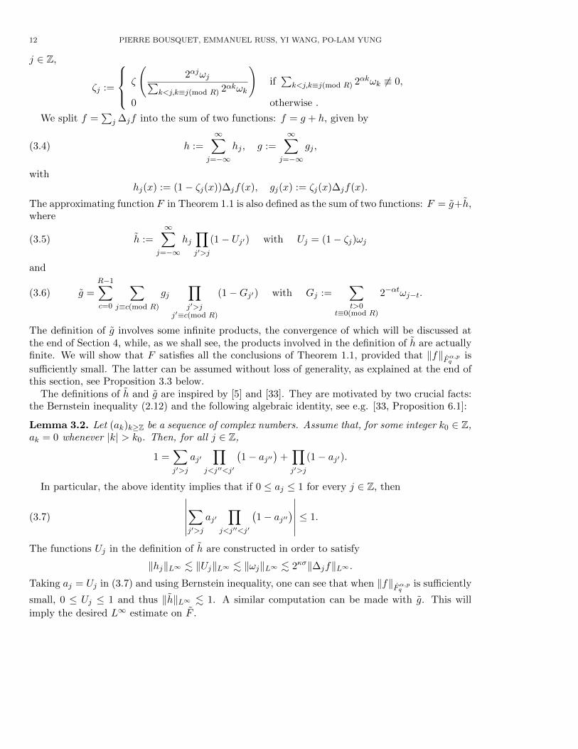
12 PIERRE BOUSQUET, EMMANUEL RUSS, YI WANG, PO-LAM YUNG
j ∈ Z,
ζj :=
ζ
(2αjωj∑
k<j,k≡j(mod R) 2αkωk
)if∑
k<j,k≡j(mod R) 2αkωk 6≡ 0,
0 otherwise .
We split f =∑
j ∆jf into the sum of two functions: f = g + h, given by
(3.4) h :=∞∑
j=−∞hj , g :=
∞∑j=−∞
gj ,
with
hj(x) := (1− ζj(x))∆jf(x), gj(x) := ζj(x)∆jf(x).
The approximating function F in Theorem 1.1 is also defined as the sum of two functions: F = g+h,where
(3.5) h :=∞∑
j=−∞hj∏j′>j
(1− Uj′) with Uj = (1− ζj)ωj
and
(3.6) g =
R−1∑c=0
∑j≡c(mod R)
gj∏j′>j
j′≡c(mod R)
(1−Gj′) with Gj :=∑t>0
t≡0(mod R)
2−αtωj−t.
The definition of g involves some infinite products, the convergence of which will be discussed atthe end of Section 4, while, as we shall see, the products involved in the definition of h are actuallyfinite. We will show that F satisfies all the conclusions of Theorem 1.1, provided that ‖f‖Fα,pq
is
sufficiently small. The latter can be assumed without loss of generality, as explained at the end ofthis section, see Proposition 3.3 below.
The definitions of h and g are inspired by [5] and [33]. They are motivated by two crucial facts:the Bernstein inequality (2.12) and the following algebraic identity, see e.g. [33, Proposition 6.1]:
Lemma 3.2. Let (ak)k≥Z be a sequence of complex numbers. Assume that, for some integer k0 ∈ Z,ak = 0 whenever |k| > k0. Then, for all j ∈ Z,
1 =∑j′>j
aj′∏
j<j′′<j′
(1− aj′′
)+∏j′>j
(1− aj′).
In particular, the above identity implies that if 0 ≤ aj ≤ 1 for every j ∈ Z, then
(3.7)
∣∣∣∣∣∣∑j′>j
aj′∏
j<j′′<j′
(1− aj′′
)∣∣∣∣∣∣ ≤ 1.
The functions Uj in the definition of h are constructed in order to satisfy
‖hj‖L∞ . ‖Uj‖L∞ . ‖ωj‖L∞ . 2κσ‖∆jf‖L∞ .Taking aj = Uj in (3.7) and using Bernstein inequality, one can see that when ‖f‖Fα,pq
is sufficiently
small, 0 ≤ Uj ≤ 1 and thus ‖h‖L∞ . 1. A similar computation can be made with g. This will
imply the desired L∞ estimate on F .
APPROXIMATION IN FRACTIONAL SOBOLEV SPACES AND HODGE SYSTEMS 13
Regarding the Fα,pq estimates, the strategies for h and g follow two different paths. For everyx ∈ Rd, h(x) is the sum of the largest Littlewood-Paley projections |∆jf(x)|. Roughly speaking,this is exploited to reduce the sum of these projections to only one term. More specifically, we willuse the following fact:
(3.8)∑m∈Z
2αmωmχ2αmωm>12
∑k<m,k≡m(mod R) 2αkωk
≤ 3R supm∈Z
2αmωm.
Indeed, writing∑m∈Z
2αmωmχ2αmωm>12
∑k<m,k≡m(mod R) 2αkωk
=R−1∑j=0
∑m≡j(mod R)
2αmωmχ2αmωm>12
∑k<m,k≡j(mod R) 2αkωk
,
we consider for every j = 0, . . . , R−1 the largest index mj in the sum∑
m≡j( mod R) · · · above such
that the corresponding term 2αmωmχ2αmωm>12
∑k<m,k≡j(mod R) 2αkωk
is > 0 (such an index mj exists
since we have assumed that only finitely many ∆kf are different from 0). Then∑m≡j(mod R)
2αmωmχ2αmωm>12
∑k<m,k≡m(mod R) 2αkωk
≤ 2αmjωmj +∑
k<mj ,k≡j(mod R)
2αkωk
≤ 3 · 2αmjωmj ≤ 3 supm∈Z
2αmωm
from which (3.8) follows. The estimate of the Fα,pq norm of the right hand side of (3.8) is the most
delicate part in the Fα,pq approximation of h by h. This is the object of Proposition 4.7 below. Letus also mention that the good derivatives play a central role in this first part of the approximation.
The Fα,pq estimate of g − g is less elaborate. As explained in the introduction, it is obtainedusing Littlewood-Paley inequalities. Here, the role of R becomes crucial.
In order to carry out the above arguments rigorously, we need to assume that ‖f‖Fα,pqis suffi-
ciently small. This is not a restriction since Theorem 1.1 is a consequence of the following (appar-ently weaker) statement:
Proposition 3.3. Let α > 0 and p, q ∈ (1,∞) such that αp = d. Let κ be the largest positiveinteger that satisfies κ < min{p, d}. Then for every δ > 0, there exists ηδ > 0 such that for every
f ∈ Fα,pq (Rd) with ‖f‖Fα,pq≤ ηδ, there exist F ∈ Fα,pq ∩ L∞(Rd) and a constant Dδ > 0 with Dδ
independent of f , such that
(3.9)κ∑i=1
‖∂i(f − F )‖Fα−1,pq
≤ δ‖f‖Fα,pq+Dδ‖f‖2Fα,pq
,
and
(3.10) ‖F‖L∞ + ‖F‖Fα,pq≤ Dδ.
We proceed to explain how Proposition 3.3 implies Theorem 1.1. Let δ > 0. By Proposition 3.3,there exist ηδ > 0 and Dδ > 0 satisfying the above properties.
Let f ∈ Fα,pq , f 6≡ 0. We then apply Proposition 3.3 to the function
f :=min
(ηδ,
δDδ
)‖f‖Fα,pq
f.
14 PIERRE BOUSQUET, EMMANUEL RUSS, YI WANG, PO-LAM YUNG
We thus obtain a function F which satisfies (3.9) and (3.10), with f instead of f . Finally, we set
F :=‖f‖Fα,pq
min(ηδ,
δDδ
) F .Then multiplying the estimates by ‖f‖Fα,pq
/min(ηδ,
δDδ
)and using that
∥∥∥f∥∥∥Fα,pq
= min(ηδ,
δDδ
)yields
κ∑i=1
‖∂i(f − F )‖Fα−1,pq
≤ δ‖f‖Fα,pq+Dδ min
(ηδ,
δ
Dδ
)‖f‖Fα,pq
≤ 2δ‖f‖Fα,pq,
and
‖F‖L∞ + ‖F‖Fα,pq≤ Dδ
min(ηδ,
δDδ
)‖f‖Fα,pq.
This proves Theorem 1.1 with Cδ = Dδ/2/min(ηδ/2,
δ2Dδ/2
).
A word about notations is in order. In the above, we have defined the functions Ej , Tj , ∆j , ωj ,ζj , hj , gj , Uj and Gj . Morally speaking, all these are localized in frequency to |ξ| . 2j . Some likeEj , Tj and ∆j are L1-renormalized dilations of a fixed function (in particular, we note in passingthat they satisfy
‖Ej‖Lp = 2jdp′ ‖E‖Lp
for all p; similarly for Tj and ∆j). The others are not dilations of a fixed function, but if we take
k derivatives of ωj , ζj , hj , gj , Uj or Gj , we can obtain an upper bound that involves a factor 2jk.This will be made explicit in the next three sections, which are devoted to the proof of Proposition3.3.
4. Properties of ωj
In this section, we collect all the estimates of ωj needed in the sequel.
4.1. Pointwise estimates. First we have (see [33, Section 9]):
Proposition 4.1. For all j ∈ Z and all x ∈ Rd,
(4.1) ωj(x) '
∑r∈Zd
(Tj |∆jf |(x+ 2−jr)E(r)
)p1/p
(4.2) |∆jf |(x) . ωj(x).
The proof of Proposition 4.1 relies on the following estimate for the function T defined in (3.2):
Lemma 4.2. For every x, y ∈ Rd, if ‖y‖ ≤√d, then T (x+ y) . T (x).
Proof of Lemma 4.2: Note that T (x) ≥ (2√d)−(d+1) for all x ∈ Rd with ‖x‖ ≤ 2
√d. Thus
T (x+ y) ≤ 1 ≤ (2√d)d+1T (x)
whenever ‖x‖ ≤ 2√d. On the other hand, if ‖x‖ > 2
√d and ‖y‖ ≤
√d, then ‖x+ y‖ ≥ ‖x‖/2, so
T (x+ y) = ‖x+ y‖−(d+1) ≤ 2d+1‖x‖−(d+1) = 2d+1T (x).
This shows T (x+ y) ≤ CT (x) with C = (2√d)d+1. �

APPROXIMATION IN FRACTIONAL SOBOLEV SPACES AND HODGE SYSTEMS 15
Proof of Proposition 4.1: The proof of (4.1) is analogous to the one of [33, Proposition 9.2]. Theonly difference is that the function Sj+N introduced in [33] is now replaced by the function Tjwhich satisfies the same (crucial) property as Sj+N , namely: for every x, y ∈ Rd, if ‖y‖ ≤ 2−j
√d,
(4.3) Tj(x+ y) ' Tj(x).
In turn, this follows from the definition of Tj and Lemma 4.2. From (4.3) one deduces that
(4.4) Tj |∆jf |(x− 2−j(y + r)) ' Tj |∆jf |(x− 2−jr)
whenever x ∈ Rd, r ∈ Zd and ‖y‖ ≤√d. Arguing as in the proof of [33, Proposition 9.2], we rewrite
ωj as
ωj(x) =
∑r∈Zd
(Tj |∆jf |(x− 2−j(y + r))E(y + r))p
1/p
where y ∈ [0, 1)d is the ‘fractional part’ of 2jx. In particular, ‖y‖ ≤√d. The estimate (4.1) then
follows from (4.4) and the fact that whenever r ∈ Zd,(4.5) E(y + r) ' E(r).
Let now K be a Schwartz function on Rd, whose Fourier transform K is identically 1 on B2, andvanishes outside B3. Then by (2.1), for every ξ ∈ Rd,
∆(ξ)K(ξ) = ∆(ξ).
Hence, ∆jf = ∆jf ∗Kj where Kj(x) = 2jdK(2jx) for all x ∈ Rd. Moreover, since K ∈ S, there
exists C > 0 such that, for all x ∈ Rd, |K(x)| ≤ CT (x). We deduce therefrom |Kj | ≤ CTj and thus
|∆jf(x)| ≤ |∆jf | ∗ |Kj |(x) ≤ C|∆jf | ∗ Tj(x).
In view of (4.1), this gives the desired conclusion |∆jf(x)| . ωj(x).�
We also have:
Proposition 4.3. (1) For all j ∈ Z,
(4.6) ωj . 2κσMM∆jf.
(2) For all j ∈ Z,
(4.7) ‖ωj‖L∞ . 2κσ‖∆jf‖L∞ . 2κσ‖f‖Fα,pq.
Proof. From (4.1), we deduce
ωj(x) .∑r∈Zd
Tj |∆jf |(x+ 2−jr)E(r).
Using (4.4) and (4.5), we get
ωj(x) .∑r∈Zd
∫(0,1)d
Tj |∆jf |(x+ 2−j(r + y))E(r + y) dy = EjTj |∆jf |(x).
We then observe that Tj |∆jf |(x) .M|∆jf |(x) and thus EjTj |∆jf |(x) . 2κσM (Tj |∆jf |). Bothare consequences of (2.9). This proves the first item. The second item is now an easy consequenceof (4.6) and the Bernstein inequality (2.12). �
16 PIERRE BOUSQUET, EMMANUEL RUSS, YI WANG, PO-LAM YUNG
The derivative estimates for ωj can be obtained in a similar manner to the proofs of [33, Propo-sition 9.6] and [33, Proposition 9.7] and they depend on how many derivatives are computed in thegood directions x′ := (x1, . . . , xκ).
Proposition 4.4. For every γ′ ∈ Nκ and γ ∈ Nd,
(4.8) |∂γ∂γ′
x′ωj | . 2(|γ′|+|γ|)j2−|γ′|σωj .
The implicit constant may depend on |γ| and |γ′| but neither on j nor on f .
Proof. We can assume that ωj 6≡ 0, and thus ωj(x) > 0 for all x ∈ Rd, see Remark 3.1. The
function u : x 7→(1 + ‖x‖2
)1/2is the Euclidean norm of the vector (1, x) in Rd+1. By homogeneity,
it follows that |∂γu(x)| . 1 for all γ ∈ Nd \ {0}. By the Faa di Bruno formula (i.e. the expressionof the iterated derivatives of the composition of two functions), we obtain the pointwise estimate|∂γ(exp ◦(pu))(x)| . exp ◦(pu)(x). By definition of E, see (3.1), it follows that for every γ ∈ Nd,γ′ ∈ Nκ,
(4.9)∣∣∣∂γ∂γ′x′Ep(2jx− r)∣∣∣ . 2j(|γ|+|γ
′|)2−|γ′|σEp(2jx− r).
By definition of ωj , see (3.3), it follows that∣∣∣∂γ∂γ′x′ωpj ∣∣∣ . 2j(|γ|+|γ′|)2−|γ
′|σωpj .
Writing ωj =(ωpj
)1/p, the Faa di Bruno formula applied to the functions ωpj and t 7→ t1/p gives∣∣∣∂γ∂γ′x′ωj∣∣∣ . 2j(|γ|+|γ
′|)2−|γ′|σωj .
This proves the proposition. �
From Proposition 4.4, we deduce:
Proposition 4.5. For every γ′ ∈ Nκ and γ ∈ Nd,
|∂γ∂γ′
x′ ζj | . 2(|γ′|+|γ|)j2−|γ′|σ.
Proof. Since the result is obvious when ζj = 0, we assume that ζj 6= 0. We write
ζj(x) = ζ
(2αjωjvj
)where vj(x) =
∑k<j,k≡j(mod R) 2αkωk. By Proposition 4.4,
(4.10) |∂γ∂γ′
x′ vj | .∑k<j
k≡j(mod R)
2αk2(|γ|+|γ′|)k2−|γ′|σωk . 2(|γ|+|γ′|)j2−|γ
′|σvj .
We now prove by induction on |γ|+ |γ′| that
(4.11)
∣∣∣∣∂γ∂γ′x′ 1
vj
∣∣∣∣ . 2(|γ|+|γ′|)j2−|γ′|σ 1
vj.
APPROXIMATION IN FRACTIONAL SOBOLEV SPACES AND HODGE SYSTEMS 17
Since 0 = ∂γ∂γ′
x′ (vj · (1/vj)), the Leibniz formula implies
vj∂γ∂γ
′
x′1
vj= −
∑β≤γ,β′≤γ′
|β|+|β′|<|γ|+|γ′|
(γ
β
)(γ′
β′
)∂γ−β∂γ
′−β′x′ vj∂
β∂β′
x′
(1
vj
).
Using (4.10) and (4.11) for every |β|+ |β′| < |γ|+ |γ′|, it then follows that∣∣∣∣∂γ∂γ′x′ 1
vj
∣∣∣∣ . 1
vj
∑β≤γ,β′≤γ′
|β|+|β′|<|γ|+|γ′|
2(|γ−β|+|γ′−β′|)j2−|γ′−β′|σvj · 2(|β|+|β′|)j2−|β
′|σ 1
vj. 2(|γ|+|γ′|)j2−|γ
′|σ 1
vj.
By Leibniz formula and Proposition 4.4, this gives∣∣∣∣∂γ∂γ′x′ (2αjωjvj
)∣∣∣∣ . 2(|γ|+|γ′|)j2−|γ′|σ(
2αjωjvj
)and the desired estimate now follows from the Faa di Bruno formula applied to the functions ζ and2αjωjvj
, and also the fact that ζj(x) = 0 when 2αjωj(x) > vj(x).
�
4.2. Integral estimates. We first establish:
Proposition 4.6. For 1 < p, q <∞, α > 0,
(4.12) ‖‖(2αjωj)‖`q(j)‖Lp . 2κσ‖f‖Fα,pq
Proof. This follows from item 1 in Proposition 4.3 and (2.8). �
The key result of this section is an integral estimate on supj
(2αjωj), which will be used crucially
to bound ‖∂1(h− h)‖Fα,pqin section 5.
Proposition 4.7. One has
(4.13) ‖ supj∈Z
(2αjωj)‖Lp . σ2κσp ‖f‖Fα,pq
.
The proof of Proposition 4.7 is more involved than the previous ones. It relies on the followingestimate:
Proposition 4.8. Let p ∈ (1,∞) and q ∈ [1,∞]. Then there exists C = C(p, q, d) > 0 such thatfor every f = (fj)j∈Z ∈ Lp(Rd; `q(Z)), for every r ∈ Rd,
(4.14) ‖‖(Tj |fj |(·+ 2−jr))j∈Z‖`q(Z)‖Lp(Rd) ≤ C ln(2 + ‖r‖)‖‖(fj)j∈Z‖`q(Z)‖Lp(Rd).
The proof of Proposition 4.8 will be given in Appendix 10 below. Let us now derive Proposition4.7 from Proposition 4.8.

18 PIERRE BOUSQUET, EMMANUEL RUSS, YI WANG, PO-LAM YUNG
Proof. By Proposition 4.1, for every x ∈ Rd,
supj∈Z
(2αjωj(x))p . supj∈Z
∑r∈Zd
(2αjTj |∆jf |(x+ 2−jr)E(r))p
.∑r∈Zd
E(r)p supj∈Z
(2αjTj |∆jf |(x+ 2−jr))p
=∑r∈Zd
E(r)p
[supj∈Z
(2αjTj |∆jf |(x+ 2−jr))
]p.∑r∈Zd
E(r)p‖(2αjTj |∆jf |(x+ 2−jr))j∈Z‖p`q .
Integrating over x ∈ Rd, we get
‖ supj∈Z
2αjωj‖pLp .∑r∈Zd
E(r)p‖‖(2αjTj |∆jf |(·+ 2−jr))j∈Z‖`q‖pLp .
By Proposition 4.8, this gives
‖ supj∈Z
2αjωj‖pLp .∑r∈Zd
E(r)p[ln(2 + ‖r‖)]p‖f‖pFα,pq
.
In order to estimate∑
r∈Zd E(r)p[ln(2 + ‖r‖)]p, we first observe that for every r ∈ Zd, for every
x ∈ r + [0, 1]d,
E(r) ≤ e−‖rσ‖ ≤ e−‖rσ‖1/√d ≤ e(2−σκ+(d−κ))/
√de−‖xσ‖1/
√d.
Here ‖x‖1 is the `1-norm given by |x1|+ · · ·+ |xd|. Moreover, ln(2 + ‖r‖) ≤ ln(3 + ‖x‖1). It followsthat ∑
r∈ZdE(r)p(ln(2 + ‖r‖))p .
∫Rde−p‖xσ‖1/
√d(ln(3 + ‖x‖1))p dx
≤∫Rde−p‖xσ‖1/
√d(ln(3 + 2σ ‖xσ‖1))p dx
= 2σκ∫Rde−p‖x‖1/
√d[ln(3 + 2σ ‖x‖1)]p dx
. σp2σκ.
This completes the proof of Proposition 4.7. �
What will be important for us above is that the power of 2σ in (4.13), namely κp , is strictly less
than 1.We will use Proposition 4.7 in the following form:
Lemma 4.9.
(4.15) ‖‖2αmωmχ2αmωm>12
∑k<m,k≡m(mod R) 2αkωk
‖`q(m)‖Lp . Rσ2κσp ‖f‖Fα,pq
.
Proof. Since `1(Z) continuously embeds in `q(Z), one gets
‖‖2αmωmχ2αmωm>12
∑k<m,k≡m(mod R) 2αkωk
‖`q(m)‖Lp . ‖∑m∈Z
2αmωmχ2αmωm>12
∑k<m,k≡m(mod R) 2αkωk
‖Lp .

APPROXIMATION IN FRACTIONAL SOBOLEV SPACES AND HODGE SYSTEMS 19
It is enough to combine (3.8) with Proposition 4.7 to conclude the proof of the lemma.�
We end up this section by establishing the expected L∞ bounds on F under a smallness conditionon ‖f‖Fα,pq
. More precisely, in view of (4.2) and (4.7), there exists η > 0 such that if 2κσ ‖f‖Fα,pq≤ η,
then for every j ∈ Z‖ωj‖L∞ , ‖∆jf‖L∞ < 1.
By definition of Uj , hj and gj , see (3.4) and (3.5), this implies
(4.16) ‖Uj‖L∞ , ‖hj‖L∞ , ‖gj‖L∞ < 1.
We can also obtain L∞ bounds on Gj , h and g:
Lemma 4.10. Assume that 2κσ ‖f‖Fα,pq≤ η with η as above. Then
(1)∥∥∥h∥∥∥
L∞. 1,
(2) there exists j0 ∈ N such that for every x ∈ Rd, and every j ∈ Z,
|Gj(x)| ≤min
(2−αR, 2−α(j−j0)
)1− 2−αR
.
In particular, ‖Gj‖L∞ ≤1
2αR−1.
(3) The infinite products involved in the definition (3.6) of g are uniformly convergent on Rd.If we further assume that αR > 1, then ‖Gj‖L∞ < 1 and ‖g‖L∞ . R.
Proof. Using that
|hj(x)| = (1− ζj(x)) |∆jf(x)| . (1− ζj(x))ωj(x) = Uj(x),
and that 0 ≤ Uj ≤ 1 by the choice of η, we have∥∥∥h∥∥∥L∞.
∞∑j=−∞
Uj∏j′>j
(1− Uj′)
which implies the first item by (3.7). We now estimate Gj . Let j0 ∈ N be an index for which∆jf ≡ 0 for all j > j0. Then ωj ≡ 0 for all j > j0. By the choice of η, ‖ωj‖L∞ < 1 for every j ∈ Z.
It follows that for every x ∈ Rd,
0 ≤ Gj(x) <∑
t>0,j−t≤j0t≡0(mod R)
2−αt ≤∑k≥k0
2−αRk
where k0 is the lowest positive integer such k0R ≥ j − j0. This implies
Gj(x) ≤ 2−αRk0
1− 2−αR≤
min(2−αR, 2−α(j−j0)
)1− 2−αR
and the second item follows.Moreover, whenever j > j0, ‖Gj‖L∞(Rd) . 2−α(j−j0) (with an implicit constant depending on R)
from which we obtain the uniform convergence of∏j′>j
j′≡c(mod R)
(1−Gj′) on Rd for all j. This implies
20 PIERRE BOUSQUET, EMMANUEL RUSS, YI WANG, PO-LAM YUNG
the first part of the third item. Finally, in order to obtain the estimate for g, we assume thatαR > 1. By the second item, this implies ‖Gj‖L∞ < 1. We next observe that when ζj(x) > 0,
2αjωj(x) ≤∑k<j
k≡j(mod R)
2αkωk
and thus
(4.17) |gj(x)| . ζj(x)ωj(x) .∑k<j
k≡j(mod R)
2α(k−j)ωk = Gj .
It then follows that
‖g‖L∞ .R−1∑c=0
∑j≡c(mod R)
Gj∏j′>j
j′≡c(mod R)
(1−Gj′) . R.
This completes the proof. �
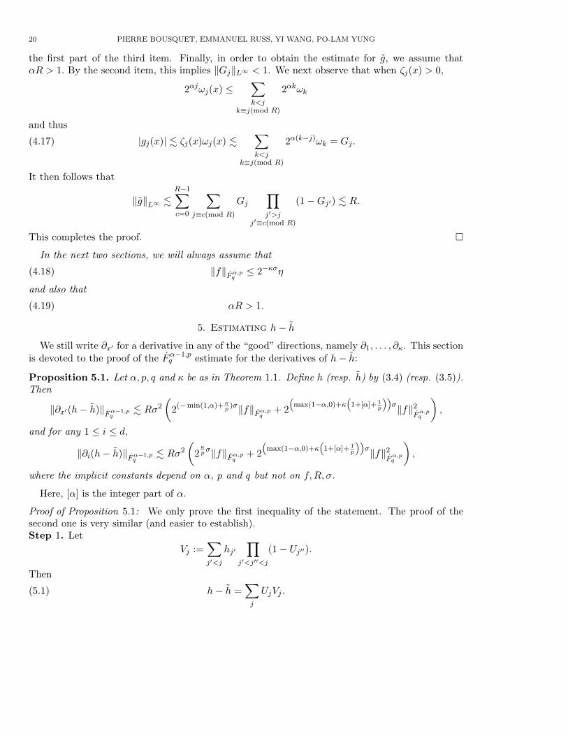
In the next two sections, we will always assume that
(4.18) ‖f‖Fα,pq≤ 2−κση
and also that
(4.19) αR > 1.
5. Estimating h− h
We still write ∂x′ for a derivative in any of the “good” directions, namely ∂1, . . . , ∂κ. This sectionis devoted to the proof of the Fα−1,p
q estimate for the derivatives of h− h:
Proposition 5.1. Let α, p, q and κ be as in Theorem 1.1. Define h (resp. h) by (3.4) (resp. (3.5)).Then
‖∂x′(h− h)‖Fα−1,pq
. Rσ2
(2
(−min(1,α)+κp
)σ‖f‖Fα,pq+ 2
(max(1−α,0)+κ
(1+[α]+ 1
p
))σ‖f‖2
Fα,pq
),
and for any 1 ≤ i ≤ d,
‖∂i(h− h)‖Fα−1,pq
. Rσ2
(2κpσ‖f‖Fα,pq
+ 2
(max(1−α,0)+κ
(1+[α]+ 1
p
))σ‖f‖2
Fα,pq
),
where the implicit constants depend on α, p and q but not on f,R, σ.
Here, [α] is the integer part of α.
Proof of Proposition 5.1: We only prove the first inequality of the statement. The proof of thesecond one is very similar (and easier to establish).Step 1. Let
Vj :=∑j′<j
hj′∏
j′<j′′<j
(1− Uj′′).
Then
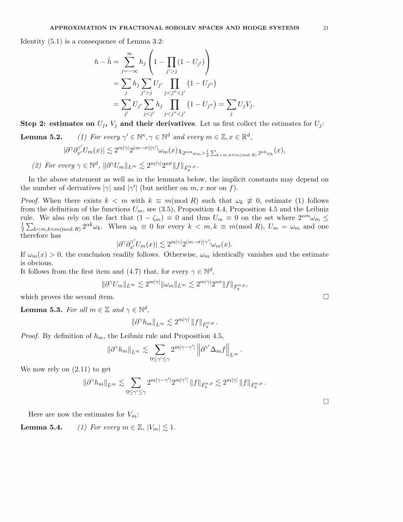
(5.1) h− h =∑j
UjVj .
APPROXIMATION IN FRACTIONAL SOBOLEV SPACES AND HODGE SYSTEMS 21
Identity (5.1) is a consequence of Lemma 3.2:
h− h =∞∑
j=−∞hj
1−∏j′>j
(1− Uj′)
=∑j
hj∑j′>j
Uj′∏
j<j′′<j′
(1− Uj′′
)=∑j′
Uj′∑j<j′
hj∏
j<j′′<j′
(1− Uj′′
)=∑j
UjVj .
Step 2: estimates on Uj, Vj and their derivatives. Let us first collect the estimates for Uj :
Lemma 5.2. (1) For every γ′ ∈ Nκ, γ ∈ Nd and every m ∈ Z, x ∈ Rd,
|∂γ∂γ′
x′Um(x)| . 2m|γ|2(m−σ)|γ′|ωm(x)χ2αmωm>12
∑k<m,k≡m(mod R) 2αkωk
(x),
(2) For every γ ∈ Nd, ‖∂γUm‖L∞ . 2m|γ|2κσ‖f‖Fα,pq.
In the above statement as well as in the lemmata below, the implicit constants may depend onthe number of derivatives |γ| and |γ′| (but neither on m,x nor on f).
Proof. When there exists k < m with k ≡ m(mod R) such that ωk 6≡ 0, estimate (1) followsfrom the definition of the functions Um, see (3.5), Proposition 4.4, Proposition 4.5 and the Leibnizrule. We also rely on the fact that (1 − ζm) ≡ 0 and thus Um ≡ 0 on the set where 2αmωm ≤12
∑k<m,k≡m(mod R) 2αkωk. When ωk ≡ 0 for every k < m, k ≡ m(mod R), Um = ωm and one
therefore has|∂γ∂γ
′
x′Um(x)| . 2m|γ|2(m−σ)|γ′|ωm(x).
If ωm(x) > 0, the conclusion readily follows. Otherwise, ωm identically vanishes and the estimateis obvious.It follows from the first item and (4.7) that, for every γ ∈ Nd,
‖∂γUm‖L∞ . 2m|γ|‖ωm‖L∞ . 2m|γ|2κσ‖f‖Fα,pq,
which proves the second item. �
Lemma 5.3. For all m ∈ Z and γ ∈ Nd,
‖∂γhm‖L∞ . 2m|γ| ‖f‖Fα,pq.
Proof. By definition of hm, the Leibniz rule and Proposition 4.5,
‖∂γhm‖L∞ .∑
0≤γ′≤γ2m|γ−γ
′|∥∥∥∂γ′∆mf
∥∥∥L∞
.
We now rely on (2.11) to get
‖∂γhm‖L∞ .∑
0≤γ′≤γ2m|γ−γ
′|2m|γ′| ‖f‖Fα,pq
. 2m|γ| ‖f‖Fα,pq.
�
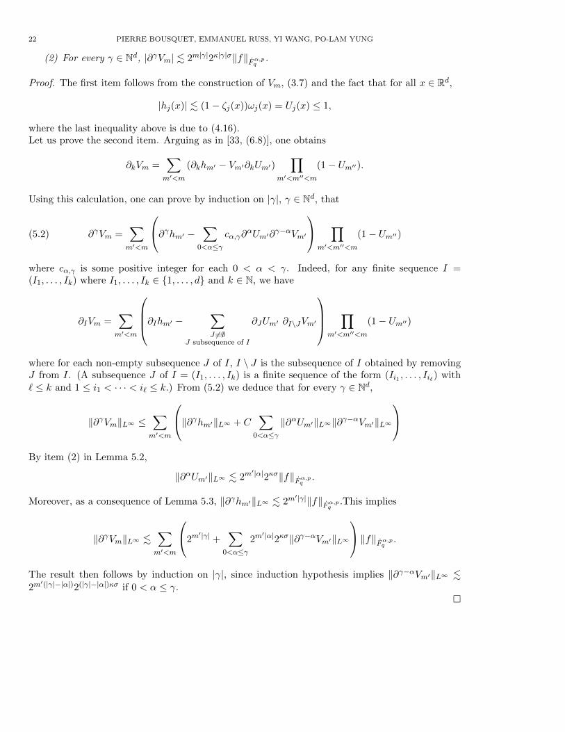
Here are now the estimates for Vm:
Lemma 5.4. (1) For every m ∈ Z, |Vm| . 1.
22 PIERRE BOUSQUET, EMMANUEL RUSS, YI WANG, PO-LAM YUNG
(2) For every γ ∈ Nd, |∂γVm| . 2m|γ|2κ|γ|σ‖f‖Fα,pq.
Proof. The first item follows from the construction of Vm, (3.7) and the fact that for all x ∈ Rd,
|hj(x)| . (1− ζj(x))ωj(x) = Uj(x) ≤ 1,
where the last inequality above is due to (4.16).Let us prove the second item. Arguing as in [33, (6.8)], one obtains
∂kVm =∑m′<m
(∂khm′ − Vm′∂kUm′)∏
m′<m′′<m
(1− Um′′).
Using this calculation, one can prove by induction on |γ|, γ ∈ Nd, that
(5.2) ∂γVm =∑m′<m
∂γhm′ − ∑0<α≤γ
cα,γ∂αUm′∂
γ−αVm′
∏m′<m′′<m
(1− Um′′)
where cα,γ is some positive integer for each 0 < α < γ. Indeed, for any finite sequence I =(I1, . . . , Ik) where I1, . . . , Ik ∈ {1, . . . , d} and k ∈ N, we have
∂IVm =∑m′<m
∂Ihm′ − ∑J 6=∅
J subsequence of I
∂JUm′ ∂I\JVm′
∏m′<m′′<m
(1− Um′′)
where for each non-empty subsequence J of I, I \ J is the subsequence of I obtained by removingJ from I. (A subsequence J of I = (I1, . . . , Ik) is a finite sequence of the form (Ii1 , . . . , Ii`) with` ≤ k and 1 ≤ i1 < · · · < i` ≤ k.) From (5.2) we deduce that for every γ ∈ Nd,
‖∂γVm‖L∞ ≤∑m′<m
‖∂γhm′‖L∞ + C∑
0<α≤γ‖∂αUm′‖L∞‖∂γ−αVm′‖L∞
By item (2) in Lemma 5.2,
‖∂αUm′‖L∞ . 2m′|α|2κσ‖f‖Fα,pq
.
Moreover, as a consequence of Lemma 5.3, ‖∂γhm′‖L∞ . 2m′|γ|‖f‖Fα,pq
.This implies
‖∂γVm‖L∞ .∑m′<m
2m′|γ| +
∑0<α≤γ
2m′|α|2κσ‖∂γ−αVm′‖L∞
‖f‖Fα,pq.
The result then follows by induction on |γ|, since induction hypothesis implies ‖∂γ−αVm′‖L∞ .2m′(|γ|−|α|)2(|γ|−|α|)κσ if 0 < α ≤ γ.
�

APPROXIMATION IN FRACTIONAL SOBOLEV SPACES AND HODGE SYSTEMS 23
Step 3 Completion of the proof of Proposition 5.1. From (5.1) we see that
‖∂x′(h− h)‖Fα−1,pq
= ‖‖2(α−1)m∆m(∂x′(h− h))‖`q(m)‖Lp
= ‖‖2(α−1)m∆m(∂x′∑j∈Z
UjVj)‖`q(m)‖Lp
= ‖‖2(α−1)m∆m(∂x′∑r∈Z
Ur+mVr+m)‖`q(m)‖Lp .
By the triangle inequality, this gives
(5.3) ‖∂x′(h− h)‖Fα−1,pq
≤∑r∈Z‖‖2(α−1)m∆m(∂x′(Ur+mVr+m))‖`q(m)‖Lp .
We now introduce a positive integer T to be defined later and we split the sum into three partsthat we estimate separately:
∑r>T . . .,
∑0≤r≤T . . . and
∑r<0 . . ..
5.1. Estimate of∑
r>T . In this case, we let ∂x′ differentiate the Littlewood-Paley projection ∆m.By Lemma 9.1 below and the fact that ‖Vm‖L∞ . 1 (Lemma 5.4),
‖‖2(α−1)m∆m(∂x′(Ur+mVr+m))‖`q(m)‖Lp . ‖‖2(α−1)m2mUr+mVr+m‖`q(m)‖Lp. 2−αr‖‖2αmUm‖`q(m)‖Lp .(5.4)
By Lemma 4.9, and the definition of Uj ,
‖‖2αmUm‖`q(m)‖Lp . ‖‖2αmωmχ2αmωm>12
∑k<m,k≡m(mod R) 2αkωk
‖`q(m)‖Lp
. Rσ2κσp ‖f‖Fα,pq
.
Hence, by summing over r > T , one gets∑r>T
‖‖2(α−1)m∆m(∂x′(Ur+mVr+m))‖`q(m)‖Lp . Rσ2−αT+κσ
p ‖f‖Fα,pq.
5.2. Estimate of∑
r<0. Let a be the integer part of α. By Lemma 9.2 and (2.3), there exist
Schwartz functions ∆(γ) such that
∆ =∑|γ|=a
∂γ∆(γ).
Then
∆m(x) = 2md∆(2mx) =∑|γ|=a
2md[∂γ∆(γ)](2mx) = 2−ma∑|γ|=a
∂γ [(∆(γ))m](x)
where (∆(γ))m(x) = 2md∆(γ)(2mx). Hence,
‖‖2(α−1)m∆m(∂x′(Um+rVm+r))‖`q(m)‖Lp
≤∑|γ|=a
‖‖2(α−1−a)m∂γ [(∆(γ))m](∂x′(Um+rVm+r))‖`q(m)‖Lp
=∑|γ|=a
‖‖2(α−1−a)m(∆(γ))m(∂(γ)∂x′(Um+rVm+r))‖`q(m)‖Lp
.∑|γ|=a
‖‖2(α−1−a)m(∂γ∂x′(Um+rVm+r))‖`q(m)‖Lp .
(5.5)
24 PIERRE BOUSQUET, EMMANUEL RUSS, YI WANG, PO-LAM YUNG
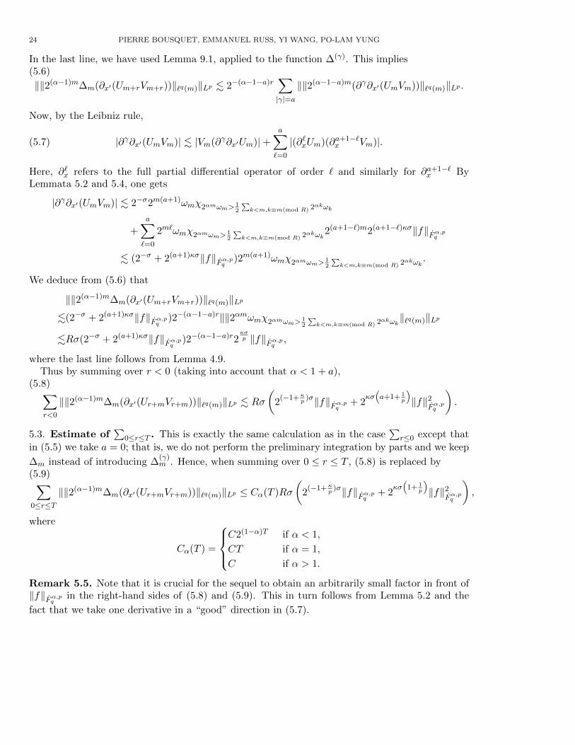
In the last line, we have used Lemma 9.1, applied to the function ∆(γ). This implies(5.6)
‖‖2(α−1)m∆m(∂x′(Um+rVm+r))‖`q(m)‖Lp . 2−(α−1−a)r∑|γ|=a
‖‖2(α−1−a)m(∂γ∂x′(UmVm))‖`q(m)‖Lp .
Now, by the Leibniz rule,
(5.7) |∂γ∂x′(UmVm)| . |Vm(∂γ∂x′Um)|+a∑`=0
|(∂`xUm)(∂a+1−`x Vm)|.
Here, ∂`x refers to the full partial differential operator of order ` and similarly for ∂a+1−`x By
Lemmata 5.2 and 5.4, one gets
|∂γ∂x′(UmVm)| . 2−σ2m(a+1)ωmχ2αmωm>12
∑k<m,k≡m(mod R) 2αkωk
+a∑`=0
2m`ωmχ2αmωm>12
∑k<m,k≡m(mod R) 2αkωk
2(a+1−`)m2(a+1−`)κσ‖f‖Fα,pq
. (2−σ + 2(a+1)κσ‖f‖Fα,pq)2m(a+1)ωmχ2αmωm>
12
∑k<m,k≡m(mod R) 2αkωk
.
We deduce from (5.6) that
‖‖2(α−1)m∆m(∂x′(Um+rVm+r))‖`q(m)‖Lp
.(2−σ + 2(a+1)κσ‖f‖Fα,pq)2−(α−1−a)r‖‖2αmωmχ2αmωm>
12
∑k<m,k≡m(mod R) 2αkωk
‖`q(m)‖Lp
.Rσ(2−σ + 2(a+1)κσ‖f‖Fα,pq)2−(α−1−a)r2
κσp ‖f‖Fα,pq
,
where the last line follows from Lemma 4.9.Thus by summing over r < 0 (taking into account that α < 1 + a),
(5.8)∑r<0
‖‖2(α−1)m∆m(∂x′(Ur+mVr+m))‖`q(m)‖Lp . Rσ(
2(−1+κ
p)σ‖f‖Fα,pq
+ 2κσ(a+1+ 1
p
)‖f‖2
Fα,pq
).
5.3. Estimate of∑
0≤r≤T . This is exactly the same calculation as in the case∑
r≤0 except that
in (5.5) we take a = 0; that is, we do not perform the preliminary integration by parts and we keep
∆m instead of introducing ∆(γ)m . Hence, when summing over 0 ≤ r ≤ T , (5.8) is replaced by
(5.9)∑0≤r≤T
‖‖2(α−1)m∆m(∂x′(Ur+mVr+m))‖`q(m)‖Lp ≤ Cα(T )Rσ
(2
(−1+κp
)σ‖f‖Fα,pq+ 2
κσ(
1+ 1p
)‖f‖2
Fα,pq
),
where
Cα(T ) =
C2(1−α)T if α < 1,
CT if α = 1,
C if α > 1.
Remark 5.5. Note that it is crucial for the sequel to obtain an arbitrarily small factor in front of‖f‖Fα,pq
in the right-hand sides of (5.8) and (5.9). This in turn follows from Lemma 5.2 and the
fact that we take one derivative in a “good” direction in (5.7).
APPROXIMATION IN FRACTIONAL SOBOLEV SPACES AND HODGE SYSTEMS 25
5.4. Conclusion. From the three above subsections, one gets, with a = [α],
(1) When α > 1, one can take T =∞:
‖∂x′(h− h)‖Fα−1,pq
. Rσ
(2
(−1+κp
)σ‖f‖Fα,pq+ 2
κσ(a+1+ 1
p
)‖f‖2
Fα,pq
).
(2) When α = 1, one can take T = σ, which implies
‖∂x′(h− h)‖Fα−1,pq
. Rσ
(σ2
(−1+κp
)σ‖f‖Fα,pq+ σ2
κσ(
2+ 1p
)‖f‖2
Fα,pq
).
(3) When 0 < α < 1, one can take T = σ, which yields
‖∂x′(h− h)‖Fα−1,pq
. Rσ
(2−(α−κ
p)σ‖f‖Fα,pq
+ 2
(1−α+κ
(1+ 1
p
))σ‖f‖2
Fα,pq
).
Altogether this proves Proposition 5.1. �
6. Estimating g − g
Proposition 6.1. Let α, p, q be as in Theorem 1.1. Define g (resp. g) by (3.4) (resp. (3.6)). Wealso introduce a number aα ∈ (0, α] such that aα <
α1−α when α < 1 and aα = 1 when α ≥ 1. Then
(6.1) ‖∂x(g − g)‖Fα−1,pq
.(
2κσR2−min(1,αaα)R‖f‖Fα,pq+ 2([α]+2)κσR22−min(1,αaα)R‖f‖2
Fα,pq
).
where the implicit constant depends on α and aα, p, q but not on f,R, σ.
Recall that [α] is the integer part of α. Also, we have written ∂x for any partial derivative ∂i,1 ≤ i ≤ d.
Remark 6.2. Note that, contrary to Proposition 5.1, we do not state an improved estimate forthe derivatives in the good directions.
Step 1. Let
Hj :=∑j′<j
j′≡j(mod R)
gj′∏
j′<j′′<jj′′≡j(mod R)
(1−Gj′′).
Then, as in Step 1 of the proof of Proposition 5.1,
g − g =∑j
GjHj .
Step 2 Estimates on Gm, Hm and their derivatives. Let us collect the upper bounds forGm and Hm which will be needed in the sequel (see [33, Propositions 11.2-11.7]). In the lemmatabelow, the implicit constants may depend on |γ| but neither on m, σ, R nor on f .
Lemma 6.3. For all m ∈ Z and all γ ∈ Nd,
|∂γGm| . 2κσ∑t>0
t≡0(mod R)
2−αt2|γ|(m−t)MM∆m−tf.
26 PIERRE BOUSQUET, EMMANUEL RUSS, YI WANG, PO-LAM YUNG
Proof. By definition of Gm, see (3.6), and Proposition 4.4, one has
|∂γGm| ≤∑t>0
t≡0(mod R)
2−αt |∂γωm−t| .∑t>0
t≡0(mod R)
2−αt2|γ|(m−t)ωm−t.
By (4.6), this implies
|∂γGm| . 2κσ∑t>0
t≡0(mod R)
2−αt2|γ|(m−t)MM∆m−tf.
�
Lemma 6.4. For all m ∈ Z and all γ ∈ Nd,
|∂γgm| . 2|γ|mM∆mf.
Proof. By definition of gm see (3.4), the Leibniz rule and Proposition 4.5,
|∂γgm| .∑
0≤γ′≤γ2|γ−γ
′|m∣∣∣∂γ′∆mf
∣∣∣ .We now rely on (2.10) to get
|∂γgm| .∑
0≤γ′≤γ2|γ−γ
′|m2|γ′|mM∆mf . 2|γ|mM∆mf.
�
Lemma 6.5. For all m ∈ Z and all γ ∈ Nd,
|Hm| . 1 , |∂γHm| . 2|γ|κσ∑t>0
t≡0(mod R)
2|γ|(m−t)MM∆m−tf.
Proof. In order to prove the estimate on |Hm|, we recall that under the conditions (4.18) and (4.19),0 ≤ Gj ≤ 1. In view of (4.17), namely |gj(x)| . Gj(x), this, in conjunction with (3.7), implies|Hm(x)| . 1.
For the second estimate, we argue by induction, assuming the correct bound for∣∣∣∂γ′Hm
∣∣∣ with
|γ′| < |γ|. We have the analogue of (5.2) for Hm in place of Vm:
∂γHm =∑m′<m
m′≡m(mod R)
∂γgm′ − ∑0<γ′≤γ
cγ′,γ∂γ′Gm′∂
γ−γ′Hm′
∏m′<m′′<m
m′′≡m(mod R)
(1−Gm′′).
Thus
|∂γHm| .∑m′<m,
m′≡m(mod R)
|∂γgm′ |+∑m′<m,
m′≡m(mod R)
∑0<γ′≤γ
∣∣∣∂γ′Gm′∂γ−γ′Hm′
∣∣∣ = I + II.
In view of Lemma 6.4,
I .∑t>0
t≡0(mod R)
2|γ|(m−t)MM(∆m−tf).

APPROXIMATION IN FRACTIONAL SOBOLEV SPACES AND HODGE SYSTEMS 27
Using instead Lemma 6.3 and the induction assumption, we get
II . 2|γ|κσ∑m′<m,
m′≡m(mod R)
∑0<γ′≤γ
∑t>0, l>0,
t≡l≡0(mod R)
2−αt2|γ′|(m′−t)MM∆m′−tf · 2|γ−γ
′|(m′−l)MM∆m′−lf
= 2|γ|κσ∑m′<m,
m′≡m(mod R)
2|γ|m′ ∑
0<γ′≤γ
∑t>0, l>0,
t≡l≡0(mod R)
2−αt2−|γ′|tMM∆m′−tf · 2−|γ−γ
′|lMM∆m′−lf.
We split the innermost sum into two parts according to whether t > l or l ≥ t and estimate by 1the factor MM∆m′−tf and MM∆m′−lf respectively (remember that ‖∆mf‖L∞ < 1 under thecondition (4.18)); this gives∑
t>0, l>0,t≡l≡0(mod R)
2−αt2−|γ′|tMM∆m′−tf · 2−|γ−γ
′|lMM∆m′−lf .∑t>0,
t≡0(mod R)
2−αt2−|γ|tMM∆m′−tf.
Finally,
II . 2|γ|κσ∑m′<m,
m′≡m(mod R)
2|γ|m′ ∑
t>0,t≡0(mod R)
2−αt2−|γ|tMM∆m′−tf
= 2|γ|κσ∑l>0,
l≡0(mod R)
∑t>0,
t≡0(mod R)
2−αt2|γ|(m−l−t)MM∆m−l−tf.
We sum this double sum by first summing over the pairs (t, l) where l + t is constant, and thensum over the remaining variable. This gives the desired conclusion. �
Step 3 Completion of the proof. As in the proof of (5.3),
‖∂x(g − g)‖Fα−1,pq
≤∑r∈Z‖‖2(α−1)m∆m(∂x(Gr+mHr+m))‖`q(m)‖Lp .
By definition of Gr+m (see (3.6)) and the triangle inequality,
‖∂x(g − g)‖Fα−1,pq
≤∑t>0,
t≡0(mod R)
2−αt∑r∈Z‖‖2(α−1)m∆m(∂x(ωr+m−tHr+m))‖`q(m)‖Lp .
For each fixed t, we now split the sum over r into three parts as follows∑r∈Z· · · =
∑r≤0
· · ·+∑
0<r<aαt
· · ·+∑r≥aαt
. . . ,
where aα > 0 was defined in Proposition 6.1. We proceed to estimate the three terms separately.
6.1. Estimate of∑
r≥aαt. As in the proof of (5.4) we integrate by parts to let ∂x hit ∆m, and use
‖Hm‖L∞ . 1 to get
‖‖2(α−1)m∆m(∂x(ωr+m−tHr+m))‖`q(m)‖Lp . 2−α(r−t)‖‖2αmωm‖`q(m)‖Lp .
This implies
‖‖2(α−1)m∆m(∂x(ωr+m−tHr+m))‖`q(m)‖Lp . 2κσ2−α(r−t)‖f‖Fα,pq,

28 PIERRE BOUSQUET, EMMANUEL RUSS, YI WANG, PO-LAM YUNG
by Proposition 4.6. Summing over r and t, one gets∑t>0
t≡0(mod R)
∑r≥aαt
2−αt‖‖2(α−1)m∆m(∂x(ωr+m−tHr+m))‖`q(m)‖Lp . 2κσ
∑t≥R
∑r≥aαt
2−αr
‖f‖Fα,pq
. 2κσ2−αaαR‖f‖Fα,pq.(6.2)
6.2. Estimate of∑
r≤0. Let a ≥ 0 be an integer. Arguing as for the proof of (5.6), we write ∆m
as an a-th derivative and integrate by parts to hit ∂x(ωm+r−tHm+r), and obtain(6.3)
‖‖2(α−1)m∆m(∂x(ωm+r−tHm+r))‖`q(m)‖Lp . 2−(α−1−a)r‖‖2(α−1−a)m(∂a+1x (ωm−tHm))‖`q(m)‖Lp .
Here ∂a+1x refer to the full partial differential operator of order a+ 1.
We now use the fact that for every ` ∈ N
ωm−t . 2κσMM(∆m−tf) , |∂`xωm−t| . 2(m−t)`ωm−t
(see Propositions 4.3 and 4.4) and also for k ∈ N∗
|Hm| . 1 , |∂kxHm| . 2kκσ∑t′>0
2(m−t′)kMM∆m−t′f
(see Lemma 6.5). By the Leibniz rule, this implies
|∂a+1x (ωm−tHm)| . 2(m−t)(a+1)ωm−t+2(a+2)κσ
∑t′>0
a∑`=0
2(t′−t)`2(a+1)(m−t′)MM∆m−tf ·MM∆m−t′f.
We split the sum over t′ into two parts according to whether t′ ≤ t or t′ > t and we estimate by‖f‖Fα,pq
the factor MM∆m−tf or MM∆m−t′f respectively (here we use (2.12)):∑t′>0
a∑`=0
2(t′−t)`2(a+1)(m−t′)MM∆m−tf · MM∆m−t′f
. ‖f‖Fα,pq
∑0<t′≤t
2(a+1)(m−t′)MM∆m−t′f +∑t′>t
2(t′−t)a2(a+1)(m−t′)MM∆m−tf
. ‖f‖Fα,pq
∑0<t′≤t
2(a+1)(m−t′)MM∆m−t′f.
Putting these together,
|∂a+1x (ωm−tHm)| . 2(m−t)(a+1)ωm−t + 2(a+2)κσ‖f‖Fα,pq
∑0<t′≤t
2(a+1)(m−t′)MM∆m−t′f.
Setting Ba,α(t) :=∑
0<t′≤t 2(α−1−a)t′ , we deduce that
‖‖2(α−1−a)m(∂a+1x (ωm−tHm))‖`q(m)‖Lp
.2(α−1−a)t‖‖2α(m−t)ωm−t‖`q(m)‖Lp + 2(a+2)κσ‖f‖Fα,pq
∑0<t′≤t
2−(a+1)t′‖‖2αmMM∆m−t′f‖`q(m)‖Lp
.2(α−1−a)t‖‖2αmωm‖`q(m)‖Lp + 2(a+2)κσ‖f‖Fα,pqBa,α(t)‖‖2αmMM∆mf‖`q(m)‖Lp

APPROXIMATION IN FRACTIONAL SOBOLEV SPACES AND HODGE SYSTEMS 29
By Proposition 2.5, this implies
‖‖2(α−1−a)m(∂a+1x (ωm−tHm))‖`q(m)‖Lp
.2(α−1−a)t‖‖2αmωm‖`q(m)‖Lp + 2(a+2)κσ‖f‖Fα,pqBa,α(t)‖‖2αm∆mf‖`q(m)‖Lp
≤2κσ2(α−1−a)t‖f‖Fα,pq+Ba,α(t)2(a+2)κσ‖f‖2
Fα,pq,
where the last line is a consequence of Proposition 4.6.Coming back to (6.3), we get(6.4)
‖‖2(α−1)m∆m(∂x(ωm+r−tHm+r))‖`q(m)‖Lp . 2−(α−1−a)r(
2κσ2(α−1−a)t‖f‖Fα,pq+Ba,α(t)2(a+2)κσ‖f‖2
Fα,pq
).
Choose now a = [α], so that Ba,α(t) . 1. Summing up on r ≤ 0, which is possible since α−a−1 < 0,we thus obtain∑
r≤0
‖‖2(α−1)m∆m(∂x(ωm+r−tHm+r))‖`q(m)‖Lp . 2κσ2(α−1−a)t‖f‖Fα,pq+ 2(a+2)κσ‖f‖2
Fα,pq.
Summing over t, we finally get
(6.5)∑t>0,
t≡0(mod R)
2−αt∑r≤0
‖‖2(α−1)m∆m(∂x(ωr+m−tHr+m))‖`q(m)‖Lp
. 2κσ2−(a+1)R‖f‖Fα,pq+ 2(a+2)κσ2−αR‖f‖2
Fα,pq.
6.3. Estimate of∑
0≤r≤aαt. Applying (6.4) with a = 0, we obtain
‖‖2(α−1)m∆m(∂x(ωm+r−tHm+r))‖`q(m)‖Lp . 2−(α−1)r(
2κσ2(α−1)t‖f‖Fα,pq+B0,α(t)22κσ‖f‖2
Fα,pq
),
where
B0,α(t) =
C if α < 1,
Ct if α = 1,
C2(α−1)t if α > 1.
Summing on 0 ≤ r ≤ aαt, we get∑0≤r≤aαt
‖‖2(α−1)m∆m(∂x(ωm+r−tHm+r))‖`q(m)‖Lp . Aα(t)(
2κσ2(α−1)t‖f‖Fα,pq+B0,α(t)22κσ‖f‖2
Fα,pq
),
where
Aα(t) =
C2(1−α)aαt if α < 1,
Caαt if α = 1,
C if α > 1.
Summing over t, one gets∑t>0
t≡0(mod R)
2−αt∑
0≤r≤aαt‖‖2(α−1)m∆m(∂x(ωm+r−tHm+r))‖`q(m)‖Lp
.∑t≥R
2−αtAα(t)(
2κσ2(α−1)t‖f‖Fα,pq+ 22κσB0,α(t)‖f‖2
Fα,pq
).
30 PIERRE BOUSQUET, EMMANUEL RUSS, YI WANG, PO-LAM YUNG
When α > 1, one has aα = 1. Since Aα(t) = C and B0,α(t) = C2(α−1)t, this implies∑t>0,
t≡0(mod R)
2−αt∑
0≤r≤aαt‖‖2(α−1)m∆m(∂x(ωm+r−tHm+r))‖`q(m)‖Lp . 2κσ2−R‖f‖Fα,pq
+22κσ2−R‖f‖2Fα,pq
.
When α = 1, the choice aα = 1 leads to Aα(t) = Ct and B0,α(t) = Ct. Hence∑t>0,
t≡0(mod R)
2−αt∑
0≤r≤aαt‖‖2(α−1)m∆m(∂x(ωm+r−tHm+r))‖`q(m)‖Lp . 2κσR2−R‖f‖Fα,pq
+22κσR22−R‖f‖2Fα,pq
.
When α < 1, Aα(t) = C2(1−α)aαt and B0,α(t) = C. One needs to take aα <α
1−α for the sum toconverge and one gets∑
t>0,t≡0(mod R)
2−αt∑
0≤r≤aαt‖‖2(α−1)m∆m(∂x(ωm+r−tHm+r))‖`q(m)‖Lp
. 2κσ2−R(1−(1−α)aα)‖f‖Fα,pq+ 22κσ2−R(α−(1−α)aα)‖f‖2
Fα,pq.
In any case, for every α > 0, and assuming further that aα ≤ α when α < 1, we have
(6.6)∑t>0,
t≡0(mod R)
2−αt∑
0≤r≤aαt‖‖2(α−1)m∆m(∂x(ωm+r−tHm+r))‖`q(m)‖Lp
. 2κσR2−Rmin(1,αaα)‖f‖Fα,pq+ 22κσR22−Rmin(1,αaα)‖f‖2
Fα,pq.
6.4. Conclusion. The three subsections above, namely inequalities (6.2), (6.5) and (6.6), implythe desired estimate (6.1). This completes the proof of Proposition 6.1.
7. Completion of the proof of Proposition 3.3
Let us summarize the current state of the proof. For every σ ∈ N∗, we define
R :=κ+ 1
min(1, αaα)σ
where aα has been introduced in Proposition 6.1. This automatically implies the condition (4.19)since αR ≥ (κ + 1)σ/aα > 1. Then by Lemma 4.10, Proposition 5.1 and Proposition 6.1, there
exists η > 0 such that for every f ∈ Fα,pq with ‖f‖Fα,pq≤ η2−κσ, there exists a map F = g + h in
Fα,pq such that
‖g‖L∞ . R,∥∥∥h∥∥∥
L∞. 1
and in the good directions x′:
‖∂x′(h− h)‖Fα−1,pq
. σ3
(2
(−min(1,α)+κp
)σ‖f‖Fα,pq+ 2
(max(1−α,0)+κ
(1+[α]+ 1
p
))σ‖f‖2
Fα,pq
),
while in all directions:
‖∂x(h− h)‖Fα−1,pq
. σ3
(2κpσ‖f‖Fα,pq
+ 2
(max(1−α,0)+κ
(1+[α]+ 1
p
))σ‖f‖2
Fα,pq
),
‖∂x(g − g)‖Fα−1,pq
.(σ2−σ‖f‖Fα,pq
+ σ22([α]+1)κσ‖f‖2Fα,pq
).

APPROXIMATION IN FRACTIONAL SOBOLEV SPACES AND HODGE SYSTEMS 31
In order to prove Proposition 3.3, we take for every δ > 0 an integer σ > 0 such that
σ32(−min(1,α)+κ
p)σ ≤ δ
2, σ2−σ ≤ δ
2.
This is possible in view of the fact that κp < min(1, α). This implies that
‖∂x′(f − F )‖Fα−1,pq
≤ ‖∂x′(h− h)‖Fα−1,pq
+ ‖∂x′(g − g)‖Fα−1,pq
≤ δ‖f‖Fα,pq+Dδ‖f‖2Fα,pq
for some Dδ > 0 which may depend on σ (and thus on δ). We also have
‖F‖L∞ ≤ ‖g‖L∞ +∥∥∥h∥∥∥
L∞≤ Dδ,
and using Proposition 2.3
‖F‖Fα,pq≤∥∥∥h− h∥∥∥
Fα,pq
+ ‖g − g‖Fα,pq+ ‖f‖Fα,pq
≤ Dδ,
by enlarging Dδ if necessary. This completes the proof of Proposition 3.3.
8. Solving Hodge systems
Proof of Theorem 1.2: We follow [5, p. 284]. On the space F s,pq (ΛlRd) of l-forms with coefficients
in F s,pq (Rd), we use the norm
‖λ‖F s,pq (ΛlRd) = max|I|=l‖λI‖F s,pq (Rd)
if λ =∑|I|=l λIdxI . Let ϕ ∈ Fα,pq (ΛlRd). Since d : Fα,pq (ΛlRd) → Fα−1,p
q (ΛlRd) is bounded with
closed range, by the open mapping theorem, there exists λ(0) ∈ Fα,pq (ΛlRd) such that
dλ(0) = dϕ
and
(8.1)∥∥∥λ(0)
∥∥∥Fα,pq (ΛlRd)
≤ C ‖dϕ‖Fα−1,pq (ΛlRd)
.
Choose δ > 0 such that Cδ ≤ 12 . Let I ⊂ Nd be a multi-index with length l. Theorem 1.1 provides
a function β(0)I ∈ F
α,pq (Rd) ∩ L∞(Rd) such that, for all j ∈ J1, dK \ I (note that there are at most κ
such indexes), ∥∥∥∂j (λ(0)I − β
(0)I
)∥∥∥Fα−1,pq (Rd)
≤ δ∥∥∥λ(0)
I
∥∥∥Fα,pq (Rd)
≤ Cδ ‖dϕ‖Fα−1,pq (ΛlRd)
and ∥∥∥β(0)I
∥∥∥Fα,pq (Rd)
+∥∥∥β(0)
I
∥∥∥L∞(Rd)
≤ Cδ∥∥∥λ(0)
I
∥∥∥Fα,pq (Rd)
≤ C ′δ ‖dϕ‖Fα−1,pq (ΛlRd)
.
Set β(0) :=∑
I β(0)I dxI . Then, β(0) ∈ Fα,pq (ΛlRd) ∩ L∞(ΛlRd). Moreover, since dϕ = dλ(0),∥∥∥d(ϕ− β(0))∥∥∥Fα−1,pq (ΛlRd)
= max|I|=l
maxj 6∈I
∥∥∥∂j(λ(0)I − β
(0)I )∥∥∥Fα−1,pq (ΛlRd)
≤ 1
2‖dϕ‖
Fα−1,pq (ΛlRd)
and ∥∥∥β(0)∥∥∥Fα,pq (ΛlRd)
+∥∥∥β(0)
∥∥∥L∞(ΛlRd)
≤ C ′ ‖dϕ‖Fα−1,pq (ΛlRd)
.

32 PIERRE BOUSQUET, EMMANUEL RUSS, YI WANG, PO-LAM YUNG
The same argument, applied to 2(ϕ−β(0)) instead of ϕ, yields β(1) ∈ Fα,pq (ΛlRd)∩L∞(ΛlRd) suchthat ∥∥∥β(1)
∥∥∥Fα,pq (ΛlRd)
+∥∥∥β(1)
∥∥∥L∞(ΛlRd)
≤ C ′∥∥∥2d
(ϕ− β(0)
)∥∥∥Fα−1,pq (ΛlRd)
≤ C ′ ‖dϕ‖Fα−1,pq (ΛlRd)
and ∥∥∥∥dϕ− d(β(0) +1
2β(1)
)∥∥∥∥Fα−1,pq (ΛlRd)
≤ 1
4‖dϕ‖
Fα−1,pq (ΛlRd)
.
Iterating this procedure, we construct a sequence (β(i))i≥0 ∈ Fα,pq (ΛlRd)∩L∞(ΛlRd) such that, forall N ≥ 0, ∥∥∥∥∥dϕ− d
(N∑i=0
2−iβ(i)
)∥∥∥∥∥Fα−1,pq (ΛlRd)
≤ 1
2N+1‖dϕ‖
Fα−1,pq (ΛlRd)
and ∥∥∥β(N)∥∥∥Fα,pq (ΛlRd)
+∥∥∥β(N)
∥∥∥L∞(ΛlRd)
≤ C ′ ‖dϕ‖Fα−1,pq (ΛlRd)
.
Therefore, if ψ :=∑∞
i=0 2−iβ(i), ψ satisfies all the conclusions of Theorem 1.2. �
9. Appendix: some properties of Schwartz functions
As a consequence of Proposition 2.5,
Lemma 9.1. There exists a constant C which depends only on ∆ such that for all p, q ∈ (1,∞),for all (fm)m∈Z ∈ Lp(Rd; `q(Z)), for all k ∈ N,
‖‖∂kx∆mfm‖`q(m)‖Lp ≤ C‖‖2kmfm‖`q(m)‖Lp .
For every γ = (γ1, . . . , γd) ∈ Nd, we denote
|γ| = γ1 + · · ·+ γd , ∂γ = ∂γ11 · · · ∂γdd .
Moreover, Xγ is the polynomial Xγ11 . . . Xγd
d and for every polynomial P (X1, . . . , Xd) =∑
γ aγXγ ,
P (D) is the differential operator∑
γ aγ∂γ .
Lemma 9.2. Suppose φ is a Schwartz function on Rd and m ∈ N. Assume that for every polynomialP of degree less or equal to m,
∫Rd P (x)φ(x) dx = 0. Then for every γ ∈ Nd such that |γ| = m+ 1,
there exists a Schwartz function φ(γ) such that
φ =∑
|γ|=m+1
∂γφ(γ).
Proof. In terms of the Fourier transform ψ of φ, the assumption means that ∂γψ(0) = 0 for every
|γ| ≤ m while the conclusion amounts to the existence of Schwartz functions ψ(γ) such that
ψ =∑
|γ|=m+1
ξγψ(γ).
Let η ∈ C∞c (Rd) is a smooth cut-off function with η ≡ 1 near the origin. By the Taylor formula:
∀ξ ∈ Rd, ψ(ξ) =∑
|γ|=m+1
ξγ(
1
m!
∫ 1
0(1− t)m∂γψ(tξ) dt
).
APPROXIMATION IN FRACTIONAL SOBOLEV SPACES AND HODGE SYSTEMS 33
By the identity |ξ|2(m+1) =∑|γ|=m+1 cγξ
2γ with cγ = (m+ 1)!/(γ1! . . . γd!), we also have
ψ(ξ) = η(ξ)∑
|γ|=m+1
ξγ(
1
m!
∫ 1
0(1− t)m∂γψ(tξ) dt
)+
1− η(ξ)
|ξ|2(m+1)ψ(ξ)
∑|γ|=m+1
cγξ2γ .
We can thus set
ψ(γ)(ξ) := η(ξ)
(1
m!
∫ 1
0(1− t)m∂γψ(tξ) dt
)+ cγ(1− η(ξ))
ξγ
|ξ|2(m+1)ψ(ξ).
The proof is complete.�
10. Appendix: proof of Proposition 4.8
We begin with the following result.
Proposition 10.1. Let {kj}j∈Z be a sequence of non-negative integrable functions on Rd, with
(10.1) supj∈Z‖kj‖L1(Rd) . 1
and
(10.2)
∫‖y‖≥4‖x‖
supj∈Z|kj(y − x)− kj(y)|dy ≤ A
for some constant A ≥ 1. Then the associated maximal function
(10.3) Mf := supj∈Z|f | ∗ kj
is of weak-type (1, 1), and is bounded on Lp(Rd) for all 1 < p ≤ ∞; more precisely,
(10.4) ‖Mf‖L1,∞ . A‖f‖L1
and
(10.5) ‖Mf‖Lp . A1/p‖f‖Lp , 1 < p ≤ ∞.
Also, M satisfies a vector-valued weak-L1 and strong-Lp bound, namely
(10.6) ‖‖Mfi‖`q‖L1,∞ . A‖‖fi‖`q‖L1 , 1 < q ≤ ∞,
and
(10.7) ‖‖Mfi‖`q‖Lp . A1/p‖‖fi‖`q‖Lp , 1 < p ≤ q ≤ ∞.
The first part of the statement, namely (10.4) and (10.5), is essentially in the work of Zo [35],whose proof we reproduce below. One relies on a Banach-valued version of the singular integraltheorem. To prove (10.4), we consider the Banach spaces B1 = C, B2 = `∞, and the vector-valuedsingular integral
f 7→ Tf := {f ∗ kj}j∈Zwhich is a mapping of a B1-valued function f to a B2-valued function Tf = {f ∗ kj}j∈Z. Fortechnical reasons, we consider truncations of this operator T , namely TMf := {f ∗ kj}j∈Z,|j|≤Mfor M ∈ N, and show that the operator norm ‖TM‖L1→L1,∞(`∞) is . A uniformly for M ∈ N. At

34 PIERRE BOUSQUET, EMMANUEL RUSS, YI WANG, PO-LAM YUNG
almost every point x ∈ Rd, the kernel {kj(x)}j∈Z,|j|≤M can be thought of as a linear map from B1
to B2, whose operator norm is supj∈Z,|j|≤M |kj(x)|, and we note that the latter is in L1(Rd) since
(10.8)
∫Rd
supj∈Z,|j|≤M
|kj(x)|dx ≤∫Rd
∑j∈Z,|j|≤M
|kj(x)|dx .M.
Since TM : L∞ → L∞(`∞) with norm . 1, the vector-valued singular integral theorem ([2, Theorem4.2]) gives
‖TM‖L1→L1,∞(`∞) . A,
and interpolation in turn gives
‖TM‖Lp→Lp(`∞) . A1/p
for all 1 < p < ∞. Both bounds being independent of M , we obtain (10.4) and (10.5) by lettingM → +∞. Similarly, to prove (10.6), we consider the Banach spaces B1 = `q, B2 = `q(`∞), andfor each M ∈ N the vector-valued truncated singular integral
f = {fi}i∈Z 7→ TMf := {fi ∗ kj}i,j∈Z,|j|≤Mwhich is a mapping of a B1-valued function f = {fi}i∈Z to a B2-valued function TMf = {fi ∗kj}i,j∈Z,|j|≤M . The B2 norm of TMf at x is by definition∑
i∈Zsupj∈Z|j|≤M
|fi ∗ kj(x)|q
1/q
.
At almost every point x ∈ Rd, the kernel {kj(x)}j∈Z,|j|≤M can be thought of as a linear map fromB1 to B2, whose operator norm is supj∈Z,|j|≤M |kj(x)|. As before, we note that this latter expression
is in L1 for all M ∈ N. Now if 1 < q ≤ ∞ and M ∈ N, (10.5) gives TM : Lq(`q)→ Lq(`q(`∞)), with
norm . A1/q uniformly in M . Hence the vector-valued singular integral theorem gives
‖TM‖L1(`q)→L1(`q(`∞)) . A,
and interpolation in turn gives
‖TM‖Lp(`q)→Lp(`q(`∞)) . A1/p
for all 1 < p ≤ q. Therefore, (10.6) and (10.7) follow, as we let M → +∞. To apply Proposi-tion 10.1, we use the following Lemma:
Lemma 10.2. Suppose ϕ : Rd → R is a non-negative integrable function on Rd satisfying
(10.9)
∫Rdϕ(y)dy . 1,
(10.10)
∫‖y‖≥R
ϕ(y)dy . R−1 for all R ≥ 1,
and
(10.11)
∫Rd|ϕ(y − x)− ϕ(y)|dy . ‖x‖ for all x ∈ Rd with ‖x‖ ≤ 1.
Define, for all j ∈ Z and all x ∈ Rd,(10.12) ϕj(x) := 2jdϕ(2jx),
APPROXIMATION IN FRACTIONAL SOBOLEV SPACES AND HODGE SYSTEMS 35
and define, for r ∈ Rd,(10.13) kj(x) := ϕj(x+ 2−jr).
Then the kernels kj satisfy (10.2) with A . ln(2 + ‖r‖), i.e.∫‖y‖≥4‖x‖
supj∈Z|kj(y − x)− kj(y)|dy . ln(2 + ‖r‖).
Proof. The proof is a variant of the argument in [23, Chapter II, Section 4.2]. Indeed, it suffices toreplace the sup by a sum, and show that
(10.14)
∫‖y‖≥4‖x‖
∑j∈Z|kj(y − x)− kj(y)|dy . ln(2 + ‖r‖).
We assume ‖r‖ ≥ 2, for the case ‖r‖ < 2 follows from a simple modification of the followingargument. We split the sum into three parts:
∑j∈Z =
∑2j‖x‖≤1 +
∑1<2j‖x‖<‖r‖+
∑2j‖x‖≥‖r‖.
The first sum can be estimated using condition (10.11):∫‖y‖≥4‖x‖
∑2j‖x‖≤1
|kj(y − x)− kj(y)|dy ≤∫Rd
∑2j‖x‖≤1
2jd|ϕ(2j(y − x) + r)− ϕ(2jy + r)|dy
=
∫Rd
∑2j‖x‖≤1
|ϕ(y − 2jx+ r)− ϕ(y + r)|dy
.∑
2j‖x‖≤1
2j‖x‖
. 1.
The second sum can be estimated using condition (10.9):∫‖y‖≥4‖x‖
∑1<2j‖x‖<‖r‖
|kj(y − x)− kj(y)|dy ≤∑
1<2j‖x‖<‖r‖
2
∫Rdkj(y)dy
= 2∑
1<2j‖x‖<‖r‖
∫Rdϕ(y)dy
. log ‖r‖.The last sum can be estimated using condition (10.10):∫
‖y‖≥4‖x‖
∑2j‖x‖≥‖r‖
|kj(y − x)− kj(y)|dy ≤∑
2j‖x‖≥‖r‖
2
∫‖y‖≥2‖x‖
kj(y)dy
=∑
2j‖x‖≥‖r‖
2
∫‖y‖≥2·2j‖x‖
ϕ(y + r)dy
.∑
2j‖x‖≥‖r‖
1
2j‖x‖
.1
‖r‖. 1.
Altogether we get (10.14). �

36 PIERRE BOUSQUET, EMMANUEL RUSS, YI WANG, PO-LAM YUNG
Combining Proposition 10.1 and Lemma 10.2, we see that:
Corollary 10.3. If ϕ is as in Lemma 10.2, r ∈ Rd, and ϕj, kj and M are as defined as in (10.12),
(10.13) and (10.3) respectively, then M is bounded on Lp with norm . [ln(2 + ‖r‖)]1/p, and itsatisfies the vector-valued estimate
(10.15) ‖‖Mfi‖`q‖Lp . [ln(2 + ‖r‖)]1/p‖‖fi‖`q‖Lp , 1 < p ≤ q ≤ ∞.
The above statement is reminiscent of similar estimates in the scalar-valued case [23, ChapterII.5.10] and [20, Theorem 4.1]. See also [14, Theorem 3.1] for a more general vector-valued estimate,that includes the case p > q.We are now in position to prove Proposition 4.8. We apply Corollary 10.3 when ϕ = T , whereT (x) := min(1, ‖x‖−(d+1)) as in (3.2). We first verify conditions (10.9), (10.10) and (10.11) withT in place of ϕ. Indeed (10.9) and (10.10) are obvious, and (10.11) follows since if x ∈ Rd with‖x‖ ≤ 1, then∫
Rd|T (y − x)− T (y)|dy ≤
∫1−‖x‖≤‖y‖≤1+‖x‖
2dy +
∫‖y‖≥1+‖x‖
∣∣∣∣ 1
‖y − x‖d+1− 1
‖y‖d+1
∣∣∣∣ dy. ‖x‖+
∫‖y‖≥1+‖x‖
‖x‖‖y‖d+2
dy
. ‖x‖,where the first inequality relies on the fact that T (y − x) = T (y) = 1 when ‖y‖ ≤ 1 − ‖x‖while in the second inequality we have used the mean value theorem to estimate the integrand (if‖y‖ ≥ 1 + ‖x‖ and ‖x‖ ≤ 1, then ‖y‖ ≥ 2‖x‖, so ‖y − tx‖ ≥ ‖y‖/2 for all t ∈ [0, 1], hence thedesired estimate). Hence Corollary 10.3 applies. Now for any r ∈ Rd and any j ∈ Z, we haveTj |fj |(x + 2−jr) = |fj | ∗ kj(x) ≤ Mfj(x) for all x ∈ Rd. Hence from Corollary 10.3, we concludethat
‖‖(Tj |fj |(·+ 2−jr))j∈Z‖`q(Z)‖Lp(Rd) . [ln(2 + ‖r‖)]1p ‖‖(fj)j∈Z‖`q(Z)‖Lp(Rd) if 1 < p ≤ q ≤ ∞.
Duality between Lp(`q) and Lp′(`q′) then shows that
‖‖(Tj |fj |(·+ 2−jr))j∈Z‖`q(Z)‖Lp(Rd) . [ln(2 + ‖r‖)]1p′ ‖‖(fj)j∈Z‖`q(Z)‖Lp(Rd) if 1 ≤ q ≤ p <∞.
Since both [ln(2 + ‖r‖)]1p and [ln(2 + ‖r‖)]
1p′ are bounded from above by ln(2 + ‖r‖), (4.14) then
follows.
References
[1] Cherif Amrouche and Huy Hoang Nguyen. New estimates for the div-curl-grad operators and elliptic problemswith L1-data in the whole space and in the half-space. J. Differential Equations, 250(7):3150–3195, 2011.
[2] A. Benedek, A. P. Calderon, and R. Panzone. Convolution operators on Banach space valued functions. Proc.Nat. Acad. Sci., 48(3):356–365, 1962.
[3] Gerard Bourdaud, Madani Moussai, and Winfried Sickel. Composition operators on Lizorkin-Triebel spaces. J.Funct. Anal., 259(5):1098–1128, 2010.
[4] Jean Bourgain and Haım Brezis. On the equation div Y = f and application to control of phases. J. Amer. Math.Soc., 16(2):393–426, 2003.
[5] Jean Bourgain and Haım Brezis. New estimates for elliptic equations and Hodge type systems. J. Eur. Math.Soc. (JEMS), 9(2):277–315, 2007.
[6] Pierre Bousquet, Petru Mironescu, and Emmanuel Russ. A limiting case for the divergence equation. Math. Z.,274(1-2):427–460, 2013.

APPROXIMATION IN FRACTIONAL SOBOLEV SPACES AND HODGE SYSTEMS 37
[7] Pierre Bousquet and Jean Van Schaftingen. Hardy-Sobolev inequalities for vector fields and canceling lineardifferential operators. Indiana Univ. Math. J., 63(5):1419–1445, 2014.
[8] Haım Brezis and Jean Van Schaftingen. Boundary estimates for elliptic systems with L1-data. Calc. Var. PartialDifferential Equations, 30(3):369–388, 2007.
[9] Sagun Chanillo and Jean Van Schaftingen. Subelliptic Bourgain-Brezis estimates on groups. Math. Res. Lett.,16(3):487–501, 2009.
[10] Sagun Chanillo, Jean Van Schaftingen, and Po-Lam Yung. Applications of Bourgain-Brezis inequalities to fluidmechanics and magnetism. C. R. Math. Acad. Sci. Paris, 354(1):51–55, 2016.
[11] Sagun Chanillo, Jean Van Schaftingen, and Po-Lam Yung. Bourgain–Brezis inequalities on symmetric spaces ofnon-compact type. J. Funct. Anal., 273(4):1504–1547, 2017.
[12] Sagun Chanillo, Jean Van Schaftingen, and Po-Lam Yung. Variations on a proof of a borderline Bourgain-BrezisSobolev embedding theorem. Chin. Ann. Math. Ser. B, 38(1):235–252, 2017.
[13] Sagun Chanillo and Po-Lam Yung. An improved Strichartz estimate for systems with divergence free data.Comm. Partial Differential Equations, 37(2):225–233, 2012.
[14] Shaoming Guo, Jonathan Hickman, Victor Lie, and Joris Roos. Maximal operators and Hilbert transforms alongvariable non-flat homogeneous curves. Proc. London Math. Soc., 115:117–219, 2017.
[15] Loredana Lanzani and Elias M. Stein. A note on div curl inequalities. Math. Res. Lett., 12(1):57–61, 2005.[16] Vladimir Maz’ya. Bourgain-Brezis type inequality with explicit constants. In Interpolation theory and applica-
tions, volume 445 of Contemp. Math., pages 247–252. Amer. Math. Soc., Providence, RI, 2007.[17] Vladimir Maz’ya. Estimates for differential operators of vector analysis involving L1-norm. J. Eur. Math. Soc.
(JEMS), 12(1):221–240, 2010.[18] Petru Mironescu. On some inequalities of Bourgain, Brezis, Maz’ya, and Shaposhnikova related to L1 vector
fields. C. R. Math. Acad. Sci. Paris, 348(9-10):513–515, 2010.[19] Irina Mitrea and Marius Mitrea. A remark on the regularity of the div-curl system. Proc. Amer. Math. Soc.,
137(5):1729–1733, 2009.[20] Camil Muscalu. Calderon commutators and the Cauchy integral on Lipschitz curves revisited: I. First commu-
tator and generalizations. Rev. Mat. Iberoam., 30(2):727–750, 2014.[21] Thomas Runst and Winfried Sickel. Sobolev spaces of fractional order, Nemytskij operators, and nonlinear partial
differential equations, volume 3 of de Gruyter Series in Nonlinear Analysis and Applications. Walter de Gruyter& Co., Berlin, 1996.
[22] Elias M. Stein. Singular integrals and differentiability properties of functions. Princeton Mathematical Series,No. 30. Princeton University Press, Princeton, N.J., 1970.
[23] Elias M. Stein. Harmonic analysis: real-variable methods, orthogonality, and oscillatory integrals, volume 43 ofPrinceton Mathematical Series. Princeton University Press, Princeton, NJ, 1993. With the assistance of TimothyS. Murphy; Monographs in Harmonic Analysis, III.
[24] Eitan Tadmor. Hierarchical construction of bounded solutions in critical regularity spaces. Comm. Pure Appl.Math., 69(6):1087–1109, 2016.
[25] Hans Triebel. Theory of function spaces, volume 78 of Monographs in Mathematics. Birkhauser Verlag, Basel,1983.
[26] Jean Van Schaftingen. Estimates for L1-vector fields. C. R. Math. Acad. Sci. Paris, 339(3):181–186, 2004.[27] Jean Van Schaftingen. A simple proof of an inequality of Bourgain, Brezis and Mironescu. C. R. Math. Acad.
Sci. Paris, 338(1):23–26, 2004.[28] Jean Van Schaftingen. Function spaces between BMO and critical Sobolev spaces. J. Funct. Anal., 236(2):490–
516, 2006.[29] Jean Van Schaftingen. Estimates for L1 vector fields under higher-order differential conditions. J. Eur. Math.
Soc. (JEMS), 10(4):867–882, 2008.[30] Jean Van Schaftingen. Limiting fractional and Lorentz space estimates of differential forms. Proc. Amer. Math.
Soc., 138(1):235–240, 2010.[31] Jean Van Schaftingen. Limiting Sobolev inequalities for vector fields and canceling linear differential operators.
J. Eur. Math. Soc. (JEMS), 15(3):877–921, 2013.[32] Jean Van Schaftingen. Limiting Bourgain-Brezis estimates for systems of linear differential equations: theme
and variations. J. Fixed Point Theory Appl., 15(2):273–297, 2014.[33] Yi Wang and Po-Lam Yung. A subelliptic Bourgain-Brezis inequality. J. Eur. Math. Soc. (JEMS), 16(4):649–693,
2014.
38 PIERRE BOUSQUET, EMMANUEL RUSS, YI WANG, PO-LAM YUNG
[34] Po-Lam Yung. Sobolev inequalities for (0, q) forms on CR manifolds of finite type. Math. Res. Lett., 17(1):177–196, 2010.
[35] Felipe Zo. A note on approximation of the identity. Studia Math., 55(2):111–122, 1976.
Pierre Bousquet:Universite Paul Sabatier, CNRS UMR 5219, Institut de Mathematiques de ToulouseF-31062 Toulouse Cedex 9, FranceE-mail address: [email protected]
Emmanuel Russ:Universite Grenoble Alpes, CNRS UMR 5582, Institut Fourier100 rue des Mathematiques, F-38610 Gieres, FranceE-mail address: [email protected]
Yi Wang:John Hopkins University, Department of Mathematics3400 N. Charles Street, 216 Krieger Hall, Baltimore, MD, 21218, USAE-mail address: [email protected]
Po Lam Yung:The Chinese University of Hong-Kong, Department of MathematicsLady Shaw Building, Ma Liu Shui, Shatin, Hong KongE-mail address: [email protected]


![Fast Iterative Solution of Elliptic Control Problems in ... · investigated, con rming the theoretical results. Keywords: Control problem, fractional Sobolev norms, ... [Br,Brm,Ha2],](https://static.fdocuments.in/doc/165x107/5af4711a7f8b9a4d4d8da4bb/fast-iterative-solution-of-elliptic-control-problems-in-con-rming-the-theoretical.jpg)


![Numerical study of time-fractional hyperbolic partial ... · advection-diffusion equation. Sousa [23] proposed an approximation of the Caputo fractional derivative of order 1 < 6](https://static.fdocuments.in/doc/165x107/5edbf1b6ad6a402d6666651a/numerical-study-of-time-fractional-hyperbolic-partial-advection-diffusion-equation.jpg)