
Approximation and Hardness: Beyond P and NP · of fine-grained complexity theory, which seeks to...
278
Approximation and Hardness: Beyond P and NP Pasin Manurangsi Electrical Engineering and Computer Sciences University of California at Berkeley Technical Report No. UCB/EECS-2019-49 http://www2.eecs.berkeley.edu/Pubs/TechRpts/2019/EECS-2019-49.html May 16, 2019
Transcript of Approximation and Hardness: Beyond P and NP · of fine-grained complexity theory, which seeks to...
Approximation and Hardness: Beyond P and NP
Pasin Manurangsi
Electrical Engineering and Computer SciencesUniversity of California at Berkeley
Technical Report No. UCB/EECS-2019-49http://www2.eecs.berkeley.edu/Pubs/TechRpts/2019/EECS-2019-49.html
May 16, 2019

Copyright © 2019, by the author(s).All rights reserved.
Permission to make digital or hard copies of all or part of this work forpersonal or classroom use is granted without fee provided that copies arenot made or distributed for profit or commercial advantage and that copiesbear this notice and the full citation on the first page. To copy otherwise, torepublish, to post on servers or to redistribute to lists, requires prior specificpermission.
Approximation and Hardness: Beyond P and NP
by
Pasin Manurangsi
A dissertation submitted in partial satisfaction of the
requirements for the degree of
Doctor of Philosophy
in
Computer Science
in the
Graduate Division
of the
University of California, Berkeley
Committee in charge:
Professor Luca Trevisan, Co-chairProfessor Prasad Raghavendra, Co-chair
Professor Nikhil Srivastrava
Spring 2019

Approximation and Hardness: Beyond P and NP
Copyright 2019by
Pasin Manurangsi
1
Abstract
Approximation and Hardness: Beyond P and NP
by
Pasin Manurangsi
Doctor of Philosophy in Computer Science
University of California, Berkeley
Professor Luca Trevisan, Co-chair
Professor Prasad Raghavendra, Co-chair
The theory of NP-hardness of approximation has led to numerous tight characterizations ofapproximability of hard combinatorial optimization problems. Nonetheless, there are many funda-mental problems which are out of reach for these techniques, such as problems that can be solved(or approximated) in quasi-polynomial time, parameterized problems and problems in P.
This dissertation continues the line of work that develops techniques to show inapproximabilityresults for these problems. In the process, we provide hardness of approximation results for thefollowing problems.
• Problems Between P and NP: Dense Constraint Satisfaction Problems (CSPs), Densestk-Subgraph with Perfect Completeness, VC Dimension, and Littlestone’s Dimension.
• Parameterized Problems: k-Dominating Set, k-Clique, k-Biclique, Densest k-Subgraph,Parameterized 2-CSPs, Directed Steiner Network, k-Even Set, and k-Shortest Vector.
• Problems in P: Closest Pair, and Maximum Inner Product.
Some of our results, such as those for Densest k-Subgraph, Directed Steiner Network and Parame-terized 2-CSP, also present the best known inapproximability factors for the problems, even in the(believed) NP-hard regime. Furthermore, our results for k-Dominating Set and k-Even Set resolvetwo long-standing open questions in the field of parameterized complexity.

i
To my parents
ii
Contents
Contents ii
1 Introduction and Overview 11.1 Part I: Problems Between P and NP . . . . . . . . . . . . . . . . . . . . . . . . . . 21.2 Part II: Parameterized Problems . . . . . . . . . . . . . . . . . . . . . . . . . . . . 61.3 Part III: Problems in P . . . . . . . . . . . . . . . . . . . . . . . . . . . . . . . . . 121.4 Discussion and Future Directions . . . . . . . . . . . . . . . . . . . . . . . . . . . 131.5 Bibliographic Notes . . . . . . . . . . . . . . . . . . . . . . . . . . . . . . . . . . 13
2 Notation, Preliminaries and Tools 152.1 Notation . . . . . . . . . . . . . . . . . . . . . . . . . . . . . . . . . . . . . . . . 152.2 Problem Definitions . . . . . . . . . . . . . . . . . . . . . . . . . . . . . . . . . . 172.3 Exponential Time Hypotheses . . . . . . . . . . . . . . . . . . . . . . . . . . . . 182.4 Fine-Grained Complexity Assumptions . . . . . . . . . . . . . . . . . . . . . . . . 202.5 Nearly-Linear Size PCPs and (Sub)exponential Time Reductions . . . . . . . . . . 212.6 Parameterized Complexity . . . . . . . . . . . . . . . . . . . . . . . . . . . . . . 232.7 Error-Correcting Codes . . . . . . . . . . . . . . . . . . . . . . . . . . . . . . . . 272.8 Zarankiewicz Problem and Related Bounds . . . . . . . . . . . . . . . . . . . . . 282.9 Well-Behaved Subsets . . . . . . . . . . . . . . . . . . . . . . . . . . . . . . . . . 292.10 Two Variants of Label Covers . . . . . . . . . . . . . . . . . . . . . . . . . . . . . 312.11 Feige’s Reduction From Label Cover to Set Cover . . . . . . . . . . . . . . . . . . 34
I Problems Between P and NP 37
3 A Birthday Repetition Theorem and Its Applications 383.1 Additional Preliminaries and Notations . . . . . . . . . . . . . . . . . . . . . . . . 453.2 Birthday Repetition Theorem and Its Proof . . . . . . . . . . . . . . . . . . . . . . 473.3 Applications of the Birthday Repetition Theorem . . . . . . . . . . . . . . . . . . 503.4 Improved Approximation Algorithm for Dense CSPs . . . . . . . . . . . . . . . . 553.5 Discussion and Open Problems . . . . . . . . . . . . . . . . . . . . . . . . . . . . 61

iii
4 Densest k-Subgraph with Perfect Completeness 634.1 The Reduction and Proofs of The Main Theorems . . . . . . . . . . . . . . . . . . 664.2 Discussion and Open Questions . . . . . . . . . . . . . . . . . . . . . . . . . . . . 73
5 VC Dimension and Littlestone’s Dimension 755.1 Interpretation of the Results . . . . . . . . . . . . . . . . . . . . . . . . . . . . . . 765.2 Additional Notations and Preliminaries . . . . . . . . . . . . . . . . . . . . . . . . 785.3 VC Dimension . . . . . . . . . . . . . . . . . . . . . . . . . . . . . . . . . . . . . 795.4 Littlestone’s Dimension . . . . . . . . . . . . . . . . . . . . . . . . . . . . . . . . 885.5 Discussion and Open Questions . . . . . . . . . . . . . . . . . . . . . . . . . . . . 98
II Parameterized Problems 100
6 Inapproximability of k-Dominating Set 1016.1 Connecting Communication Complexity and Parameterized Inapproximability: An
Overview . . . . . . . . . . . . . . . . . . . . . . . . . . . . . . . . . . . . . . . 1076.2 Additional Preliminaries . . . . . . . . . . . . . . . . . . . . . . . . . . . . . . . 1126.3 Product Space Problems and Popular Hypotheses . . . . . . . . . . . . . . . . . . 1136.4 Communication Protocols and Reduction to MAXCOV . . . . . . . . . . . . . . . 1206.5 An Efficient Protocol for Set Disjointness . . . . . . . . . . . . . . . . . . . . . . 1266.6 An Efficient Protocol for MULTI-EQUALITY . . . . . . . . . . . . . . . . . . . . . 1286.7 An Efficient Protocol for SUM-ZERO . . . . . . . . . . . . . . . . . . . . . . . . . 1306.8 Connection to Fine-Grained Complexity . . . . . . . . . . . . . . . . . . . . . . . 1316.9 Discussion and Open Questions . . . . . . . . . . . . . . . . . . . . . . . . . . . . 133
7 Inapproximability from Gap-ETH I: k-Clique and k-Induced Subgraph with Hered-itary Property 1357.1 Hardness of Approximation from MAXCOV with Projection Property . . . . . . . 1377.2 Maximum Clique . . . . . . . . . . . . . . . . . . . . . . . . . . . . . . . . . . . 1407.3 Maximum Induced Subgraph with Hereditary Properties . . . . . . . . . . . . . . 1417.4 Discussion and Open Questions . . . . . . . . . . . . . . . . . . . . . . . . . . . . 142
8 Inapproximability from Gap-ETH II: k-Biclique, k-Induced Matching on BipartiteGraphs and Densest k-Subgraph 1448.1 Rephrasing the Reduction from Chapter 4 as a Parameterized Inapproximability of
Clique-vs-Biclique . . . . . . . . . . . . . . . . . . . . . . . . . . . . . . . . . . 1468.2 Maximum Balanced Biclique . . . . . . . . . . . . . . . . . . . . . . . . . . . . . 1478.3 Densest k-Subgraph . . . . . . . . . . . . . . . . . . . . . . . . . . . . . . . . . . 1498.4 Discussion and Open Questions . . . . . . . . . . . . . . . . . . . . . . . . . . . . 150
9 Inapproximability from Gap-ETH III: Parameterized 2-CSPs, Directed SteinerNetwork, k-Unique Set Cover 152
iv
9.1 Proof Overview . . . . . . . . . . . . . . . . . . . . . . . . . . . . . . . . . . . . 1579.2 Additional Preliminaries . . . . . . . . . . . . . . . . . . . . . . . . . . . . . . . 1669.3 The Main Agreement Theorem . . . . . . . . . . . . . . . . . . . . . . . . . . . . 1679.4 Soundness Analysis of the Reduction . . . . . . . . . . . . . . . . . . . . . . . . . 1769.5 Proof of Inapproximability Results of 2-CSPs . . . . . . . . . . . . . . . . . . . . 1799.6 Inapproximability of Directed Steiner Network . . . . . . . . . . . . . . . . . . . 1829.7 Inapproximability of Unique Set Cover . . . . . . . . . . . . . . . . . . . . . . . . 1839.8 Discussion and Open Questions . . . . . . . . . . . . . . . . . . . . . . . . . . . . 186
10 Inapproximability from Gap-ETH IV: Even Set and Shortest Vector Problems 18810.1 Additional Preliminaries . . . . . . . . . . . . . . . . . . . . . . . . . . . . . . . 19210.2 Inapproximability of MLD and NVP . . . . . . . . . . . . . . . . . . . . . . . . . 19210.3 Inapproximability of k-MDP . . . . . . . . . . . . . . . . . . . . . . . . . . . . . 19410.4 Inapproximability of k-SVP: Following Khot’s Reduction . . . . . . . . . . . . . 19710.5 Discussion and Open Questions . . . . . . . . . . . . . . . . . . . . . . . . . . . . 201
IIIProblems in P 203
11 Inapproximability in P: Closest Pair and Maximum Inner Product 20411.1 Proof Overview . . . . . . . . . . . . . . . . . . . . . . . . . . . . . . . . . . . . 20711.2 Additional Preliminaries . . . . . . . . . . . . . . . . . . . . . . . . . . . . . . . 21511.3 Lower Bound on (Exact) Closest Pair under OVH . . . . . . . . . . . . . . . . . . 22011.4 Gadget Constructions . . . . . . . . . . . . . . . . . . . . . . . . . . . . . . . . . 22211.5 Inapproximability of Maximum Inner Product . . . . . . . . . . . . . . . . . . . . 22911.6 Inapproximability of Closest Pair . . . . . . . . . . . . . . . . . . . . . . . . . . . 23211.7 Inapproximability of Closest Pair in Edit Distance Metric . . . . . . . . . . . . . . 23411.8 Discussion and Open Questions . . . . . . . . . . . . . . . . . . . . . . . . . . . . 234
12 Discussion and Future Directions 237
Bibliography 243

v
Acknowledgments
Finishing up this dissertation is quite bittersweet; while I am certainly happy, the past four yearshere at Berkeley have been some of the most wonderful in my life, and I would prefer to neverleave! There are so many people I would like to thank for making this happens, and I do apologizein advance if I (inevitably) miss some.
First and foremost, I will never be able to thank my advisors, Luca Trevisan and PrasadRaghavendra, enough for what they have done for me. From their guidance when I am (com-pletely) lost to their moments of brilliance, they have truly shaped and inspired me as a researcher.Outside of theory, their perspective of the world, patience, kindness, humility–and of course greatsenses of humor–have a profound impact on me. Thank you very much Luca and Prasad!
Throughout my PhD, I have been very lucky to be mentored (and hosted) by: Dana Moshkovitz,Yury Makarychev, Madhur Tulsiani, Irit Dinur, Eden Chlamtác, Arnab Bhattacharyya, and Kai-Min Chung. I am grateful to all of them for teaching me so much, and for their continuing supportboth professionally and personally.
In addition to those listed above, I have had the great pleasure and honor to work with manyamazing collaborators, without whom this thesis would not have been possible: Karthik C.S.,Warut Suksompong, Bundit Laekhanukit, Aviad Rubinstein, Danupon Nanongkai, Haris Angeli-dakis, Parinya Chalermsook, Rajesh Chitnis, Marek Cygan, Guy Kortsarz, Daniel Reichman, IgorShinkar, Suprovat Ghoshal, Euiwoong Lee, Andreas Feldmann, Jason Li, Michal Wlodarczyk,Anupam Gupta, Aravindan Vijayaraghavan, Piotr Faliszewski, and Krzysztof Sornat. I will miss(and, in some cases, have already missed) the times we spend trying out the craziest of ideastogether!
I would also like to thank all my fellow theory students and postdocs at Berkeley for theirfriendship, our shared joyous moments–and their occasional late night companies at Soda Hall:Lynn Chua, Akshay Srinivasan, Aviad Rubinstein, Tselil Schramm, Di Wang, Jonah Brown-Cohen,Fotis Iliopoulos, Jingcheng Liu, Peihan Miao, Frank Ban, Siqi Liu, Seri Khoury, Grace Dinh,Aaron Schild, Tarun Kathuria, Sidhanth Mohanty, Chinmay Nirkhe, Arun Ganesh, Morris Yau,Elizabeth Yang, Richard Zhang, Manuel Sabin, Nick Spooner, Rotem Arnon-Friedman, Sam Hop-kins, Antonio Blanca and Sam Wong. Without you guys, this journey would not have been nearlyas fun, interesting and enjoyable!
Lastly, I thank my family, especially mom and dad, and my girlfriend, Palmy, for their unwa-vering love and support. I am most fortunate to have all of you with me throughout my life.
1
Chapter 1
Introduction and Overview
The most basic question regarding any computational problem is whether it admits an efficientalgorithm. On this front, the theory of NP-completeness [Coo71; Kar72; Leo73], arguably one ofthe most important concepts in computer science, allows us to collectively explain why thousandsof computational problems arising in wide variety of fields in science and engineering are likely tobe computationally intractable. However, while powerful, the notion of “efficiency” of algorithmsused in NP-completeness—whether their running times are polynomial in the input size—stillfalls short of providing satisfactory explanation to the complexity of a number of fundamentalproblems. For one, it fails to explain why some problems admit quasi-polynomial time algorithms,but yet do not seem to be solvable in polynomial time. Furthermore, while algorithms with runningtimes O(n) and O(n2) are both classified as efficient in this notion, the former would finish inseconds whereas the latter could take years on an input of size say 1GB, a scenario that has becomeincreasingly common in the age of big data. Such blind spots have led to a relatively new areaof fine-grained complexity theory, which seeks to understand the computational complexity ofproblems beyond whether they can be solved in polynomial time.
The aim of this thesis is to advance our understanding of optimization problems through thelens of fine-grained complexity and approximation algorithms; these are algorithms that are al-lowed to output estimated solutions rather than exact ones. Previous works have demonstrated thatsuch a relaxation can lead to a drastic change in computational complexity: some NP-hard prob-lems admit polynomial time algorithms with good approximation guarantees, and some O(n2)-time problem can be approximated well in O(n) time. However, this is not the case for everyproblem, as some problems remain intractable even when approximate solutions are allowed. Thatis, for certain approximation ratios, some NP-hard problems still do not admit polynomial timealgorithms, and some O(n2)-time problems still do not admit O(n)-time algorithms. The theoryof probabilistic checkable proofs (PCP)–which has by now been developed into the field of hard-ness of approximation–provides justifications for the first type of inapproximability: indeed, manyNP-hard problems remain NP-hard even when approximation is allowed. On the other hand, untilthe past few years, the second (fined-grained) phenomenon remained largely unexplained. Thisdissertation continues this latter body of work, and is divided into three parts, based on the com-plexity of the problems tackled: (I) problems between P and NP, (II) parameterized problems, and
CHAPTER 1. INTRODUCTION AND OVERVIEW 2
(III) problems in P. Below we provide overviews of each section. To keep the discussion at a highlevel, we will be mostly informal; all notations and results will be formalized later on in this thesis.
1.1 Part I: Problems Between P and NPFirst, as mentioned earlier, we consider problems which admits quasi-polynomial time (approxi-mation) algorithms. These problems are unlikely to be NP-hard, as otherwise all problems in NPwould be solvable in quasi-polynomial time, a scenario considered unlikely by most complexitytheorists. So how, then, can we justify the nature of these problems that lie “between P and NP”?
Similar to how polynomial-time reductions lie at the heart of the theory of NP-completeness,subexponential-time reductions play a central role in establishing computational barriers for prob-lems between P and NP. Suppose, for instance, that we would like to show that a problem Acannot be solved in N o(logN) time, where N is the size of the input. One way to do this is toreduce an instance of 3SAT with n variables to an instance of A of size N = 2O(
√n). Now, if
we had an N o(logN)-time algorithm for A , then this algorithm would have solved 3SAT in time(2O(
√n))o(
√n) = 2o(n); the latter is believed to be unlikely, a belief formalized under the name
Exponential Time Hypothesis (ETH)1 [IP01; IPZ01]. In other words, assuming ETH, we haveprovided a matching running time lower bound for problem A .
Such a reduction was arguably first pioneered in the context of hardness of approximation byAaronson, Impagliazzo and Moshkovitz [AIM14]; they dub the reduction “birthday repetition”, aname that will become clear shortly. Their reduction has since inspired hardness between P and NPfor many problems, including Densest k-Subgraph with perfect completeness [Bra+17; Man17a],Nash Equilibrium and related problems [BKW15; Rub17b; BPR16; Rub16; Bha+16b; DFS16],Community Detection [Rub17a] and VC Dimension [MR17b]. Indeed, the first part of our thesiscan be viewed as a study of the power of (variants of) birthday repetition.
1.1.1 Birthday Repetition Theorem and Dense CSPsWe start in the first chapter by considering the original birthday repetition construction from [AIM14].The reduction is most intuitive when described in terms of (one-round) two-prover games. A twoprover game G consists of
• Finite sets of questions X, Y and corresponding answer sets ΣX ,ΣY .
• A distribution Q over pairs of questions X × Y .
• A verification function P : X × Y × ΣX × ΣY → 0, 1.
The game is played as follows: the verifier picks a random pair of questions (x, y) according to thedistributionQ, and sends x to the first prover and y to the second prover. The provers then respondback with answers σx ∈ ΣX and σy ∈ ΣY ; the verifier accepts if the predicate P (x, y, σx, σy)
1See Hypothesis 1 for a more formal statement of ETH.
CHAPTER 1. INTRODUCTION AND OVERVIEW 3
evaluates to one and rejects otherwise. The goal of the provers is to select a strategy that achievesthe highest possible acceptance probability; this probability is referred to as the value of the game.
Two-prover games and, more specifically, a special class of two-prover games known as theprojection games are the starting points for reductions in a large body of hardness of approxima-tion results. In fact, the PCP Theorem [Aro+98; AS98] is equivalent to the NP-hardness of thefollowing problem: given a game, distinguish whether its value is one, or is at most 0.99.
Interestingly, the two-prover games generated by the PCP Theorem is usually “sparse”, in thesense that the support of Q is very small2 compared to |X| · |Y |. It turns out that this is not acoincidence: the “dense” case is much easier to approximate. Specifically, when Q is the uniformdistribution onX×Y (for which the game is said to be a free game), the problem of distinguishingwhether a given free game is satisfiable or whether its value is at most (1 − ε) can be solved inNO( logN
ε ) time [AIM14]3.In this light, Aaronson et al.’s birthday repetition can be viewed as a reduction from any two-
prover game to a free game that, when initialize with appropriate parameters, yields the (almost)matching N Ω(logN) running time lower bound for approximating the value of free games. Forparameters k, ` ∈ N, the (k × `)-birthday repetition Gk×` of a two-prover game G consists of
• The set of questions in Gk×` are(Xk
)and
(Y`
)respectively, i.e., each question is a subset
S ⊆ X of size k and subset T ⊆ Y of size `.
• The distribution over questions is the uniform product distribution over(Xk
)×(Y`
).
• The verifier accepts if, for every pair of (x, y) ∈ S × T such that (x, y) form a valid pair ofquestions in G, i.e., (x, y) ∈ supp(Q), the answers to x and y are accepted in G.
Notice that, for small value of k, `, say k = ` = 1, the game Gk×` is “almost trivial” because, formost of the pairs S, T , there will be no x ∈ S, y ∈ T such that (x, y) forms a valid pair of questionsin the original game G. This means that, on such (S, T ), the verifier for Gk×` always accepts.
However, the situation becomes interesting as soon as k, ` = Ω(√
N). In this regime, the
expected number of valid (x, y) for a random pair S, T is Ω(1). This is also a good point to notethat this resembles the situation of the “birthday paradox”: if there are
√D people whose birthdays
are independently identically uniformly sampled from 1, . . . , D, then the expected number ofpairs of people sharing the same birthday is Θ(1). This indeed leads Aaronson et al. [AIM14] togive the construction the name “birthday repetition”.
Under a mild non-degeneracy condition on G, the above expectation statement can be turnedinto a probabilistic guarantee that, for most S, T , there exists at least one valid (x, y) ∈ S × T . Inother words, the verifier checks at least one constraint from the original game G. Intuitively, thisshould mean that finding a good strategy for the new game Gk×` is “not easier” than that of theoriginal game G. The main contribution of [AIM14] is to confirm this intuition, by showing thatthe value of Gk×` is no more than the value of G plus O(
√k`/N).
2In fact, | supp(Q)| can be assumed to be linear in |X|+ |Y | [Tre01; Din07].3Here, we use N to denote the size of the instance, i.e., N = |X||Y ||ΣX ||ΣY |.
CHAPTER 1. INTRODUCTION AND OVERVIEW 4
In doing so, they immediately arrives at the N Ω(logN) running time lower bound for approxi-mating the value of free games: starting with a hardness of approximation result for approximatingthe value of a two-prover game G of size N , we can consider the birthday repetition game Gk×`with k = ` = Θ(
√N). The latter is of size roughly N =
(N√N
)= 2O(
√N logN). If we can approxi-
mate the value of Gk×` well in time No
(log N
log log N
), then we can approximate the value of the original
game G in time 2o(N), which would violate ETH.As readers might have already noticed, the above paragraph glosses over a subtle but important
fact: we have to start with G whose value is hard to approximate, meaning that we have to evokethe PCP Theorem to begin with. Hence, we have to also taken in the account the “size blow-up”in the PCP. Fortunately, there are known PCP constructions with small blow-ups [BS08; Din07;MR10]. Specifically, Dinur’s PCP [Din07] can produce a two-prover game (or alternatively aninstance of Gap-3SAT4) of size N = n polylog(n) when starting with a 3SAT formula of size n.As a result, the described approach still gives hardness of N Ω(log N) for approximating the value offree games.
While Aaronson et al.’s work [AIM14] appeared to have resolved the complexity of birthdayrepetition, there were in fact a few open questions remained. The main one, which was highlightedin [AIM14], is whether birthday repetition can decrease the value of a game (i.e. amplify thehardness gap). In particular, since the verifier in Gk×` checks Θ(k`/N) pairs of questions from Gin expectation, it was suggested in [AIM14] that the value of Gk×` should decrease exponentiallyin Θ(k`/N). The main contribution of our first chapter is to confirm this conjecture. In doingso, we give an almost matching running time versus approximation ratio tradeoff curve for theproblem of approximating the value of free games. Roughly speaking, we show that, to achieve anapproximation ratio of N1/i, one needs N Ω(i) time, which is tight. On a more technical level, ourproof relies in the following fact from extremal graph theory: any dense graph must contain manycopies of (small) complete bipartite subgraphs (bicliques). With this in mind, we carefully boundthe number of bicliques in the “acceptance graph” for Gk×`. This technique turns out to be usefulin the next chapter as well.
We also provide several additional results. For instance, we show a similar lower bound interms of strong SDP relaxations (i.e. the Lasserre hierarchy) and we give an approximation algo-rithm with similar running time to that of [AIM14] that works for a more general case of denseconstraint satisfaction problems (CSPs) and even when the instance might not be satisfiable.
1.1.2 Densest k-Subgraph (with Perfect Completeness)In the second chapter, we consider the DENSEST k-SUBGRAPH (DkS) with perfect completenessproblem, which can be viewed as an approximate version of the classic k-CLIQUE problem. InDkS with perfect completeness, we are given a graph G with a promise that it contains a k-clique.The goal is to find a subgraph of size k that is as dense as possible. This problem again admits
4In the Gap-3SAT problem, we are given a 3CNF formula and the goal is to distinguish between the case that it issatisfiable and the case where every assignment violates at least 1% of clauses.
CHAPTER 1. INTRODUCTION AND OVERVIEW 5
a quasi-polynomial time approximation scheme. That is, there is an nO( lognε )-time algorithm that
can find a k-vertex subgraph of density5 (1− ε) [FS97; Bar15].There is a straightforward, albeit incorrect, reduction from free games to DkS with perfect
completeness: given a free game with question sets X, Y and answer sets ΣX ,ΣY , create a graphwhose vertex set is (X×ΣX)∪(Y ×ΣY ), and two vertices (x, σx) ∈ X×ΣX and (y, σy) ∈ Y ×ΣY
are connected iff the verifier accepts (σx, σy) when the pair of questions (x, y) is drawn. The pairsof vertices whose questions are from the same set are always linked. Such a graph is sometimesreferred to as the labelled extended graph of the game. It is obvious that, if the game is satisfiable,then there is an (|X| + |Y |)-clique in the graph. Unfortunately, it is possible that the graph has adense subgraph, even when the value is very small; this reduction hence fails.
Remarkably, however, Braverman et al. [Bra+17] show that, if instead of starting from an ar-bitrary free game we start from a birthday repetition game Gk×` with k, ` = Ω(
√N), then the
reduction in fact works, in the sense that any (1 − ε)-dense subgraph of size (|X| + |Y |) (for asmall constant ε > 0) translates back to a strategy of G with high value. Similar to before, theirresult immediately implies that (1− ε)-approximation of DkS with perfect completeness requiresnΩ(logn) time assuming ETH, which nearly matches the aforementioned algorithms.
In light of our result in the previous section, it is natural to ask whether we can achieve “gapamplification” effect here as well. That is, can we prove hardness for DkS with perfect complete-ness with large factors? Unfortunately, there is a counterexample showing that this constructioncan achieve a factor of at most two (see the appendix of [Man17a]). The main contribution of thischapter is to overcome this barrier and achieve inapproximability ratios that are almost polynomial.Specifically, we show that, assuming ETH, no polynomial-time algorithm can approximates DkSwith perfect completeness to within n1/(log logn)c factor of the optimum. We also provide a finertrade-off between the approximation ratio and running time, although this is not yet tight.
Due to the mentioned counterexample, we need to modify the reduction to make our proofwork. Roughly speaking, instead of starting with two prover games, we have to start with booleanCSPs and, instead of picking sets of “questions”, we pick sets of variables instead. As alludedto above, the key step of our proof is to bound the number of (small) bicliques in the constructedgraph, which is more challenging in this case than in the previous chapter because here we areconsidering the labelled extended graph as opposed to the acceptance graph before.
Interestingly, while our proof is tailored for the special case of DkS with perfect completeness,it does give the best known hardness for DkS, in which no promise of k-clique existence is given.For the general DkS problem, Bhaskara et al.’s state-of-the-art algorithm for the problem achievesonly O(n1/4+ε) approximation ratio and it is believed that the problem is hard to approximateto within a large (possibly even polynomial) factor. Despite this, previous attempts at provinghardness of approximation, including those under average case assumptions, fail to even comeclose to a polynomial ratio; the best ratios ruled out under any worst case assumption and anyaverage case assumption were only any constant [RS10] and 2O(log2/3 n) [Alo+11] respectively.Thus, our results also present the best inapproximability factor so far for DkS.
5The density of an n-vertex graph for n > 2 is the number of its edges divided by(n2), which is a number between
zero and one (inclusive).
CHAPTER 1. INTRODUCTION AND OVERVIEW 6
1.1.3 VC Dimension and Littlestone’s DimensionThe last chapter of the first part studies the complexity of (approximating) two fundamental quan-tities in learning theory: VC Dimension and Littlestone’s Dimension. These dimensions capturethe number of samples needed in the PAC learning model and the mistake bounds in the onlinelearning model respectively. We consider the model in which a concept class is given explicitly inthe input (as a binary matrix whose (x,C)-th entry is 1 iff element x belongs to concept C), andwe would like to compute the dimensions. It is not hard to see that both quantities can be com-puted exactly in time NO(logN), where N denote the size of the input (i.e. matrix). Assuming therandomized Exponential Time Hypothesis, we prove nearly matching lower bounds on the runningtime, that hold even for approximation algorithms for small constant factors.
It should be noted that, while the constructions in this chapter are inspired by the aforemen-tioned birthday repetition, there are additional challenges, and the proof techniques also divergequite significantly from the previous ones. However, this might not be completely coincidental:while birthday repetition has found applications for very different problems, these problems allshare essentially the same quasi-polynomial time algorithm. The bottleneck in those problems isa bilinear optimization problem maxu,v u>Av, which we want to approximate to within a (small)constant additive factor. To do this, it suffices to find an O(log n)-sparse sample v of the optimalv∗; the algorithm enumerates over all sparse v’s [LMM03; Aro+12; Bar15; Che+15b]. Indeed, thealgorithms for both free games and DkS with perfect completeness are of this form.
In contrast, the problems we consider here have completely different quasi-polynomial timealgorithms: for VC Dimension, it suffices to simply enumerate over all log |C|-tuples of ele-ments (where C denotes the concept class and log |C| is the trivial upper bound on the VC di-mension) [LMR91]. Littlestone’s Dimension can be computed in quasi-polynomial time via arecursive “divide and conquer” algorithm (See Section 5.4.4). We hope that our hardness in thissection serves as a supporting evidence that the birthday repetition framework might find moreapplications for a wider range of problems in the future.
1.2 Part II: Parameterized ProblemsThe second part of this dissertation shifts the focus to the so-called parameterized complexity (ormultivariate complexity), an area which emerged in the late eighties and early nineties to pro-vide yet another approach to tackle NP-hard problems. To illustrate, let us consider three classicNP-hard problems from [Kar72]: VERTEX COVER, CLIQUE and DOMINATING SET (DOMSET).While all are NP-hard, their complexity seems to differ if we are looking to find a solution of smallsize k. In particular, whereas no N o(k)-time algorithm is known for either CLIQUE or DOMSET,this is possible in time 2k · NO(1) for VERTEX COVER; such an algorithm can be much fasterthan the trivial NO(k)-time algorithm. Motivated by this, a parameterized problem with parameterk is said to be fixed-parameter tractable (FPT) if it can be solved in f(k) · NO(1) time for some(computable) function f . This serves as the notion of “efficient algorithms” for parameterized com-plexity, in the same way that polynomial-time algorithms do in the theory of NP-completeness.
CHAPTER 1. INTRODUCTION AND OVERVIEW 7
Since its inception, parameterized complexity has provided a fruitful platform for both algo-rithmic and intractability results. Turning back to k-CLIQUE and k-DOMSET once again, the lackof FPT algorithms for them can be explained: they are complete for the classes W[1] and W[2]respectively [DF95a; DF95b]. Hence, assuming these classes do not collapse to FPT, the twoproblems are intractable in this parameterized notion. In fact, under ETH, a stronger lower boundis known: not even f(k) · N o(k)-time algorithm exists for k-CLIQUE and k-DOMSET [Che+04;Che+06]. In other words, the trivial NO(k)-time algorithm is essentially the best possible (up to theconstant in the exponent).
Approximation has been suggested as a way to overcome these parameterized complexity bar-riers. However, even when considering approximation algorithms, no “non-trivial” result is known.On the other hand, despite the strong lower bounds established for exact algorithms, few inapprox-imability results were known for parameterized problems, until the past few years.
To understand the barrier in proving hardness of approximation for parameterized problems, letus first describe the standard strategy in proving tight running time lower bounds (e.g. from [Che+04;Che+06]). These reductions can be thought of as taking an instance of 3SAT with n variables andproduces an instance of k-CLIQUE or k-DOMSET of size N = 2O(n/k). If we can solve either ofthese problems in f(k) ·N o(k) time, then we can also solve 3SAT in 2o(n) time, violating ETH.
Suppose we try to take a similar path to prove hardness of approximation. The most naturalapproach would be to first apply the PCP theorem so that we have hardness of the gap version of3SAT problem; using the best known PCP [Din07], this Gap-3SAT consists of n′ = n ·polylog(n)variables. Then, we can apply the reductions mentioned above to transform the Gap-3SAT instanceto a k-CLIQUE or k-DOMSET instance. This gives an instance of sizeN = 2O(n′/k) = 2n·polylog(n)/k.However, N is already super exponential and does not give any lower bound at all!
With this obstacle in mind, there seems to be two paths going forward: first, we can try toproduce the gap in hardness of approximation via something different than the PCP Theorem. Thefirst chapter of this second part takes this route and in the process obtain strong inapproximabilityresults for k-DOMSET, which resolves a long-standing open question in parameterized complexity.
Second, we can just make a stronger assumption, that Gap-3SAT itself takes exponential time!This assumption, now known under the name Gap-ETH, composes quite nicely with existing re-ductions. Indeed, now that there is no polylog(n) size blow-up from the PCP Theorem, applyingthe current known reductions to Gap-ETH already implies that k-CLIQUE is hard to approximate towithin a constant factor [Bon+15]. The main challenge here is thus the issue of gap amplification,e.g., how can we prove hardness of large factor for k-CLIQUE (or other problems). This is a mainfocus of this line of works, which appears in Chapters 7, 8, 9 and 10 in this dissertation.
1.2.1 Inapproximability of k-Dominating Set (via Distributed PCP)Our results for k-DOMSET (and also k-CLIQUE in the next chapter) can be best stated via thenotion of total FPT inapproximability. To motivate this notion, recall that the greedy algorithm fork-DOMSET achieves an approximation ratio of (lnn+1) [Joh74; Chv79; Lov75; Sri95; Sla96]. Inthe setting of parameterized complexity, this can be quite bad: since we think of k as much smallerthan n, then overhead factor of O(lnn) can even be unbounded in terms of k. The question, which
CHAPTER 1. INTRODUCTION AND OVERVIEW 8
has been asked multiple times in literature (see e.g. [DFM06; CGG06; Dow+08; CH10; DF13]),is whether we can get an g(k)-approximation algorithm for k-DOMSET in FPT time for somefunction g (i.e. even with say g(k) = 22k).
The main contribution of this chapter is a negative answer to this question: we show that itis W[1]-hard to approximate k-DOMSET to within g(k) factor for any function g. Furthermore,we strengthen the running time lower bounds under ETH and Strong ETH (SETH) to f(k) · nΩ(k)
and f(k) · nk−ε respectively; once again, these apply for any g(k)-approximation algorithm fork-DOMSET. In other words, there is little one can save in the running time compared to thetrivial algorithm, even when approximation is allowed. Previously, the best known hardness ofapproximation of k-DOMSET due to Chen and Lin [CL16] rules out only any constant factor andO(log1/4 k) factor under W[1]-hardness and ETH respectively.
As touched upon briefly in our above discussion, our proof uses a different way to producegap rather than the traditional approach of the PCP Theorem. In particular, we generalize the Dis-tributed PCP framework of Abboud, Rubinstein and Williams [ARW17a] for proving hardness ofapproximation in P, to the context of parameterized complexity. Roughly speaking, our generalizedview is that, if we start with a hypothesis that can be written in a certain form (see Section 6.3),then, to prove hardness of approximation for a variant of the label cover problem called MAXCOV,it suffices to give an “efficient” protocol for a certain multi-party communication problem. Thehardness of approximation for k-DOMSET is then established by reducing from the label coverproblem; such reductions were known in literature [Fei98; Cha+17] (see Section 2.11).
Stating the above connection/framework (even informally) requires a few additional notationsand hence it will be left out from the introduction; for interested readers, Section 6.1 provides abrief overview of the framework without too much notational overhead.
1.2.2 Inapproximability from Gap-ETH I: k-CliqueNext, we consider the k-CLIQUE problem. For maximization problems such as k-CLIQUE, thenotion of total inapproximability becomes slightly different. Specifically, it is now obvious to geta k-approximation for k-CLIQUE, by just outputting one vertex! As a result, such a maximizationproblem is said to be totally inapproximable if there is no o(k)-approximation in FPT time. In thischapter, we show that this is the case for k-CLIQUE. However, we need the stronger Gap-ETHassumption for this result, as opposed to just W[1] 6= FPT or ETH in the previous chapter.
On a more technical level, the proof once again proceeds by first showing hardness of MAX-COV, with a stronger requirement that the constraints have a “projection property”. Unfortunately,such a property does not hold for instances created in the previous chapter. However, we can con-struct a desirable instance relatively simply from Gap-ETH. The hardness for k-CLIQUE followsimmediately via a classic reduction from the NP-hardness of approximation literature [Fei+91].
Apart from k-CLIQUE, we also consider the problem of Maximum Induced Subgraph withHereditary Property (e.g. Maximum Induced Planar Subgraph). For this problem, Khot and Ra-man [KR00] prove a dichotomy that, for a specific property, the problem is either FPT or W[1]-hard. Here we extend this to show that, for the “hard” properties, the problem is even totallyinapproximable, assuming Gap-ETH. An interesting aspect of our reduction (from k-CLIQUE) is
CHAPTER 1. INTRODUCTION AND OVERVIEW 9
that it is noticeably simpler than that of Khot and Raman; this demonstrates that having a gap inthe starting problem can help simplify the reduction. Such a theme will come up again later in thethesis.
1.2.3 Inapproximability from Gap-ETH II: k-Biclique and Densestk-Subgraph
While the previous two chapters rely on hardness of (variants of) label cover as starting points forhardness of approximation, we take a different route in this chapter; our starting point will insteadbe the reduction from Chapter 4 (i.e. Section 1.1.2 above). As we mentioned above, the soudnessin Chapter 4 proceeds by arguing that the constructed graph contains few small bicliques. Hence,if we subsample the graph by keeping each vertex independently at random with an appropriateprobability, then, in the soundness case, the small bicliques should all disappear. It turns out thatsuch an probability is still large enough that, in the completeness case, we are left with a largeclique. In other words, this implies that the “CLIQUE-VS-BICLIQUE” problem is “totally FPTinapproximable”. This problem can then be easily reduce to k-BICLIQUE, by “bipartizing” thegraph.
It is not hard to observe that the total inapproximability of k-BICLIQUE implies some hardnessof approximation for DENEST k-SUBGRAPH, where k is the parameter. In particular, a classicresult of Kovári, Sós and Turán [KST54] says that any k-vertex graph which is t-biclique-free hasdensity at most k−Ω(1/t). Now, the total inapproximability of k-BICLIQUE implies that we cannotdistinguish in FPT time a graph containing k-biclique and one which is say (log log k)-biclique-free. Then, in the former case we have a k-vertex subgraph that has density more than a half,while in the latter any k-vertex subgraph has density at most k−Ω(1/ log log k). This gives hardnessof approximating DENSEST k-SUBGRAPH to within a factor of kO(1/ log log k). Of course, log log kcan be replaced with any function that goes to infinity as k → ∞, meaning that this approach cangives an inapproximability for DENSEST k-SUBGRAPH to within a factor of ko(1).
It should be noted however that this does not give “total FPT inapproximability” for DENEST
k-SUBGRAPH, unlike our earlier results so far. Indeed, unfortunately, we do not manage to achievetotal FPT inapproximability for any of the problems from this point onwards, although for someproblems we still get pretty strong inapproximability results.
1.2.4 Inapproximability from Gap-ETH III: Parameterized 2-CSPs withStrong Soundness (via Agreement Testing Theorem)
In an attempt to prove an even stronger hardness for DENSEST k-SUBGRAPH and related problems,we consider a harder problem (i.e. easier to prove hardness) called PARAMETERIZED 2-CSPs. Inthis context, it is easiest to described the problem in terms of the colorful version of DENEST k-SUBGRAPH. Namely, in PARAMETERIZED 2-CSP, we are given a graph G and a partition of itsvertices V (G) = V1 ∪ · · · ∪ Vk, the goal is to find k vertices each from a different partition that
CHAPTER 1. INTRODUCTION AND OVERVIEW 10
maximizes the number of edges they induced. Here k is once again the parameter. Note that thisproblem is exactly the same as DkS except that the vertices have to come from different partitions.
We show that the PARAMETERIZED 2-CSP problem is hard to approximate to within a factorof k1−o(1) assuming Gap-ETH. Interestingly, our result also gives the best known hardness of ap-proximation in terms of k, even for the non-parameterized version. In this regime, it is stronglybelieve that the problem is NP-hard to approximate to within kΩ(1) factor, but no such result isknown; in fact, proving such an NP-hardness result seems quite challenging as it would resolve awell-known conjecture in the theory of PCP called the Sliding Scale Conjecture [Bel+93]. Pleaserefer to Chapter 9 for discussions regarding the conjecture.
On a technical level, the main component in our proof is a “combinatorial agreement testingtheorem”, which can also be viewed as a derandomized direct product test. In particular, thequestion is of the following form: given boolean functions f1, . . . , fk on domains S1, . . . , Sk ⊆ [n]and suppose that δ fraction of the pairs agree on their intersections, can we recover a global functiong : [n]→ 0, 1 that “roughly” agrees with a “large” (≈ δk) fraction of the given functions? HereS1, . . . , Sk are of size Ωk(n) and are “random looking” subsets. We show that such a statementholds, even when δ is as small as 1/k1−o(1) (Theorem 9.9), which is roughly optimal since nothingnon-trivial can be said when δ 6 1/k. To the best of our knowledge, no prior derandomized directproduct tests work for such a low agreement (when measure in terms of k).
Our agreement testing theorem almost immediately yields the aforementioned hardness for 2-CSPs, by taking S1, . . . , Sk to be the subsets of the variables of the starting Gap-3SAT formula, letthe i-th partition contains every function f : Si → 0, 1, and let the constraints (i.e. edges) checkwhether the two functions agree and that they do not violate any clauses. In the completeness case,it is clear that we can pick k functions that are the restrictions of the global satisfying assignment;this yields a k-clique. On the other hand, in the soundness case, our agreement testing theoremimplies that, if δ > 1/k1−o(1) fraction of pairs of the k selected functions agree, we can recoverg : [n]→ 0, 1 that agree with many of the fi’s. When setting parameters appropriately, a simplecounting argument implies that g must satisfy almost all clauses, which is a contradiction.
There are two consequences of our hardness of approximation of PARAMETERIZED 2-CSPS:
• First, due to a known reduction [DK99; CFM18], our result implies hardness of approxima-tion for the DIRECTED STEINER NETWORK (DSN) problem with factor k1/4−o(1) where kdenotes the number of demand pairs (and k is the parameter). This is the first kΩ(1) hardnessfor the problem (even in the non-parameterized regime).
• Secondly, we show, by rephrasing our 2-CSP instance in terms of label cover with a projec-tion property and using the known reduction from label cover the set cover [Fei98], that thek-UNIQUE SET COVER is hard to approximate to within a factor of k1/2−o(1). This hardnesswill be useful in the next chapter.
Unfortunately, we still do not know how to translate the techniques developed for PARAM-ETERIZED 2-CSPs back to DkS, and even proving k0.001-factor inapproximability for the latterremains open.
CHAPTER 1. INTRODUCTION AND OVERVIEW 11
1.2.5 Inapproximability from Gap-ETH IV: k-Even Set and k-ShortestVector
In the next chapter, we consider the k-EVEN SET and k-SHORTEST VECTOR problems. The k-EVEN SET problem is a parameterized variant of the MINIMUM DISTANCE PROBLEM of linearcodes over F2, which can be stated as follows: given a generator matrix A and an integer k,determine whether the code generated by A has distance at most k, or in other words, whetherthere is a nonzero vector x such that Ax has at most k nonzero coordinates.
In the k-SHORTEST VECTOR problem, we are given a lattice whose basis vectors are integraland an integer k, and the goal is to determine whether the norm of the shortest vector (in the `pnorm for some fixed p) is at most k.
The question of whether k-EVEN SET and k-SHORTEST VECTOR are fixed-parameter tractablehas been repeatedly raised in literature; in fact, they were two of the few remaining open questionsfrom the seminal book of Downey and Fellow [DF99]. We stress here that the parameterized com-plexity of these two problems were open even for exact algorithms. In this chapter, we negativelyanswer this question by showing that, assuming Gap-ETH, there are no FPT algorithms for the twoproblems. Our lower bound holds even against approximation algorithms; the inapproximabilityratios we can rule out for k-EVEN SET is any constant factor, whereas for k-SHORTEST VECTOR
we only rule out some constant factor.Similar to the NP-hardness of approximation proofs for both problems [DMS03; Kho05], our
first step is to show that their non-homogenous counterpart, the k-NEAREST CODEWORD and k-NEAREST VECTOR problems, are hard to approximate to within large factor. This is establishedvia a known reduction of Arora et al. [Aro+97] from k-UNIQUE SET COVER, for which we showinapproximability in the previous chapter.
The second step of the proof is to reduce from hardness of approximating k-NEAREST CODE-WORD and k-NEAREST VECTOR to k-EVEN SET and k-SHORTEST VECTOR respectively. In thecase of k-SHORTEST VECTOR, the same proof as Khot’s NP-hardness proof [Kho05] works inthe parameterized settings as well. As for k-EVEN SET, the NP-hardness of approximation re-duction of Dumer, Micciancio and Sudan [DMS03] does not immediately work. While our finalreduction is still heavily inspired by their reduction, we need to define a new set of properties oferror-correcting codes, which are used as a gadget in the reduction. (See Section 10.3.1.) We thenshow that a known family of codes (in particular, the BCH code) satisfies these properties.
Once again, we stress that it is crucial to have hardness of approximation of k-NEAREST
CODEWORD and k-NEAREST VECTOR for the reductions to work. This brings us back to thepoint brought up earlier in Section 1.2.2 that starting with hardness of approximation can helpmake the reductions easier. Indeed, even if one does not care about approximation algorithms atall, obtaining hardness of approximation might still be useful in facilitating subsequent reductions,as is demonstrated here in the case of k-EVEN SET and k-SHORTEST VECTOR.
CHAPTER 1. INTRODUCTION AND OVERVIEW 12
1.3 Part III: Problems in P
1.3.1 Closest Pair and Maximum Inner ProductFinally, we consider problems within P. We mentioned above that the Distributed PCP frameworkwas developed by Abboud et al. [ARW17a] to prove hardness of approximation of problems in P.To be more specific, the canonical problems that they prove inapproximability results for are theBICHROMATIC MAXIMUM INNER PRODUCT (BMIP) and the BICHROMATIC CLOSEST PAIR
(BCP) problems [ARW17a; Rub18], which serve as the sources of other hardness results shown intheir paper(s). In both problems, we are given two setsA,B ⊆ 0, 1d of n points in d dimensions.The goal of BCP (resp. BMIP) is to find a pair of points a ∈ A,b ∈ B that minimizes (resp.maximizes) their distance ‖a− b‖2 (resp. inner product 〈a,b〉). Here we think of d as no(1). Bothproblems can be trivially solved in O(n2+o(1)) time. The results of [ARW17a; Rub18] states that,in O(n2−ε) time, BCP and BMIP cannot even be approximated to within (1 + δ) and 2log1−o(1)(n)
factors respectively where δ > 0 is a positive constant depending on ε. Their results and our resultsdiscussed below hold under the Strong Exponential Time Hypothesis (SETH); see Hypothesis 2.
As some readers might have already noticed, the “bichromatic” in the problems’ names comefrom the fact that there are two sets in the input, i.e., one for each “color”, and we are only allowedto pick one point from each color. These are different than the (originally studied) “monochro-matic” versions of the problems, where the input is just a single set and we can pick any two(distinct) points from the set. Interestingly, despite the aforementioned strong inapproximabilityresults for BCP and BMIP, it was not even known whether (monochromatic) CLOSEST PAIR
(CP) and MAXIMUM INNER PRODUCT (IP) can be solved exactly in subquadratic time. This wasindeed highlighted as an open question in several recent works [ARW17b; Wil18a; DKL18].
In this penultimate chapter, we partially answer this question by showing that for every p ∈R>1 ∪ 0, under SETH, for every ε > 0, the following holds:
• No O(n2−ε)-time algorithm can solve CP in d = (log n)Ωε(1) dimensions in the `p metric.
• There exists δ = δ(ε) > 0 such that no O(n1.5−ε)-time algorithm can approximate CP to afactor of (1 + δ) in d = Oε(log n) dimensions in the `p-metric.
• No O(n2−ε)-time algorithm can approximate MIP to within a factor of 2log1−o(1)(n) (for d =no(1) dimensions).
In particular, our first result is shown by establishing the computational equivalence of theBICHROMATIC CLOSEST PAIR problem and the (monochromatic) CLOSEST PAIR problem (up tonε factor in the running time) for d = (log n)Ωε(1) dimensions.
At the heart of all our proofs is the construction of a dense bipartite graph with low contactdimension, i.e., we construct a balanced bipartite graph on n vertices with n2−ε edges whose ver-tices can be realized as points in a (log n)Ωε(1)-dimensional Euclidean space such that every pairof vertices which have an edge in the graph are at distance exactly 1 and every other pair of ver-tices are at distance greater than 1. This graph construction is inspired by the construction of
CHAPTER 1. INTRODUCTION AND OVERVIEW 13
locally dense codes introduced by Dumer, Miccancio and Sudan in [DMS03], which was also theinspiration/template for our hardness of k-EVEN SET in the previous chapter!
1.4 Discussion and Future DirectionsAlthough we provide several open problems in each of the chapters, these are usually problemsclosely related to the study in that particular chapter. In the last chapter of this thesis (Chapter 12),we provide a more high level view of the limitations of current techniques and discuss what wefeel are interesting directions to explore in the future.
1.5 Bibliographic NotesChapter 3 is based on a work co-authored with Prasad Raghavendra which was published at ICALP2017 [MR17a]. However, the version in this thesis contains a significant improvement: the mainbirthday repetition theorem (Theorem 3.5) has better parameter dependencies and the proof iscompletely different from that in [MR17a]. The new proof in fact relies on the techniques orig-inally developed for DENSEST k-SUBGRAPH in [Man17a], on which Chapter 4 is based. Thischapter closely follows the conference version of [Man17a] published in STOC 2017, with theexception that the running time-vs-approximation ratio tradeoff is stated more explicitly here (seeTheorem 4.2). The fifth chapter is based on a joint work with Aviad Rubinstein published in COLT2017 [MR17b]; the changes from the conference version are minimal.
The sixth chapter is based on a work co-authored with Karthik C.S. and Bundit Laekhanukitfrom STOC 2018 [KLM18]. Chapters 7 and 8 are extracted from a joint work with ParinyaChalermsook, Marek Cygan, Guy Kortsarz, Bundit Laekhanukit, Danupon Nanongkai, and LucaTrevisan [Cha+17]. These three chapters follow closely to the conference versions of the papers.
The ninth chapter is based on [DM18] from ITCS 2018 co-authored with Irit Dinur. Themajor addition from there is an application for the hardness of UNIQUE SET COVER (Section 9.7).Chapter 10 is based on a joint work with Arnab Bhattacharyya, Suprovat Ghoshal and Karthik C.S. published at ICALP 2018 [Bha+18]. The main difference between the two versions is that herewe prove hardness of k-NCP and k-NVP simply by reducing from the hardness of UNIQUE SET
COVER from the previous chapter. The conference version uses a more direct reduction from 2-CSP, which yields a worse inapproximability ratio and is arguably more complicated. The proofsof hardness for k-MDP and k-SVP also contain some simplifications from a journal version inpreparation (which will be a merge between [Bha+18] and a manuscript [Bon+18] of ÉdouardBonnet, László Egri, Bingkai Lin and Dániel Marx).
Chapter 11 closely follows a joint work with Karthik C.S. from ITCS 2019 [KM19].
Excluded Works. While this dissertation includes a large part of my work, several papers haveto be (regretfully) left out of this thesis. These include works on “traditional” approximation algo-rithms and hardness of approximation [MNT16; Chl+17b; AMM17; Man17b; CM18; Man19a],
CHAPTER 1. INTRODUCTION AND OVERVIEW 14
distributed algorithms [Bec+18], subexponential and parameterized approximation algorithms [Man19b;Gup+19; MT18], and computational social choice [MS17a; MS17b; MS19a; MS19b; FSM19;Bei+19].
15
Chapter 2
Notation, Preliminaries and Tools
In this section, we provide necessary preliminaries and tools that will be used in this dissertation.Before we do so, let us first define several additional notations.
2.1 NotationFor any positive integer n, we use [n] to denote the set 1, . . . , n. For two sets X and S, defineXS to be the set of tuples (xs)s∈S indexed by S with xS ∈ X . We sometimes view each tuple(xs)s∈S as a function from S to X . For a set S and an integer n 6 |S|, we use
(Sn
)to denote the
collection of all subsets of S of size n. For convenience, we let(S0
)= ∅. We use
(S6n
)to denote(
S0
)∪ · · · ∪
(Sn
). Moreover, let P(S) :=
(S
6|S|
)denotes the power set of S.
We use exp(x) and log(x) to denote 2x and log2(x) respectively. poly(n), polylog(n), polyloglog(n)are used as a shorthand forO(nc), O((log n)c) andO((log log n)c) for some constant c respectively.Finally, Ω(f(n)) and O(f(n)) are used to denote
⋃c∈N Ω(f(n)/ logc f(n)) and
⋃c∈NO(f(n) logc f(n))
correspondingly.
2.1.1 Graph Theoretic NotationUnless state explicitly otherwise, graphs are used to referred to undirected unweighted graphs. Forany graph G, we denote by V (G) and E(G) the vertex and edge sets of G, respectively. For eachvertex u ∈ V (G), we denote the set of its neighbors by NG(v); when the graph G is clear from thecontext, we sometimes drop it from the notation. For a subset S ⊆ V (G), we use G[S] to denotethe subgraph of G induced by S; for convenience, we sometimes use E(S) to denote the set ofedges in G[S], instead of the more cumbersome notion E(G[S]). The density1 of a graph G on|V (G)| > 2 vertices is |E(G)|
(|V (G)|2 ) . We say that a graph is α-dense if its density is α.
1It is worth noting that sometimes density is defined as |E(G)|/|V (G)|. For the DENSEST-k-SUBGRAPH problem,both definitions of density result in the same objective since |S| = k is fixed. However, our notion is more convenientto deal with as it always lies in [0, 1].
CHAPTER 2. NOTATION, PRELIMINARIES AND TOOLS 16
A bipartite graph G = (U, V,E) is said to be bi-regular if every left vertex (in U ) has the samedegree, and every right vertex (in V ) has the same degree. For a parameter τ > 1, a bipartite graphis said to be τ -almost-biregular if the ratios maxu∈U deg(u)
minu∈U deg(u) and maxv∈V deg(v)minv∈V deg(v) are at most τ .
A clique of G is a complete subgraph of G; sometimes we also refer to a clique as a subsetS ⊆ V (G) such that G[S] is a clique. A biclique of G is a balanced complete bipartite subgraphof G. By k-biclique, we mean the graph Kk,k, i.e., a biclique where the number of vertices in eachpartition is k. An independent set of G is a subset of vertices S ⊆ V (G) such there is no edgejoining any pair of vertices in S. A dominating set of G is a subset of vertices S ⊆ V (G) suchthat every vertex in G is either in S or has a neighbor in S. The clique number (resp., independentnumber) of G is the size of the largest clique (resp., independent set) in G. The biclique number ofG is the largest integer k such that G contains Kk,k as a subgraph. The domination number of G isdefined similarly as the size of the smallest dominating set inG. The clique, independent and dom-ination numbers of G are usually denoted by ω(G), α(G) and γ(G), respectively. However, in thisdissertation, we will refer to these numbers by CLIQUE(G),MIS(G),DOMSET(G). Additionally,we denote the biclique number of G by BICLIQUE(G).
Moreover, for every t ∈ N, we view each element of V t as a t-size ordered multiset of V .(L,R) ∈ V t× V t is said to be a labelled copy of a t-biclique (or Kt,t) in G if, for every u ∈ L andv ∈ R, u 6= v and (u, v) ∈ E. The number of labelled copies of Kt,t in G is the number of all such(L,R)’s. It is important that we distinguish between a labelled copy of t-biclique as just defined,and a copy of t-biclique; the latter is pair of disjoint subsets L,R ⊆ V each of size t such that, forevery u ∈ L and v ∈ R, we have (u, v) ∈ E. Finally, we say that a graph is t-biclique-free if itdoes not contain a copy of t-biclique (or alternatively BICLIQUE(G) < t).
In one occasion (Section 3.2), we also use the notion of labelled copies for unbalanced bicliqueas well, which is defined similar to above. Specifically, for s, t ∈ N, (L,R) ∈ V s × V t is said tobe a labelled copy of a (s, t)-biclique (or Ks,t) in G if, for every u ∈ L and v ∈ R, u 6= v and(u, v) ∈ E.
2.1.2 Distance Measures
For any a ∈ RN , its `p norm is defined by ‖a‖p :=(∑
i∈[N ] |ai|p)1/p
for 1 6 p < ∞. Its `0 norm,denoted by ‖a‖0 is defined as |i ∈ [N ] : ai 6= 0|. It `∞ norm ‖a‖∞ is maxi∈[N ] |ai|.
The distance in the `p,`0,`∞ metric between two points a,b ∈ RN is defined as the correspond-ing norm of a − b. Sometimes we refer to `0, `2 norms/metrics as the Hamming and Euclideannorms/metrics respectively. The Hamming norm is also refered to as the Hamming weight.
We also sometimes use ∆(a) and ∆(a,b) to denote ‖a‖0 and ‖a − b‖0 respectively. Fur-thermore, we define ∆(a, S) := min
b∈S∆(a,b) for any a ∈ RN and S ⊆ RN . For a ∈ FNq and
d ∈ N, we use BN(a, d) to denote the (closed) Hamming ball of radius d centered at a, i.e.,BN(a, d) := b ∈ FNq | ∆(a,b) 6 d; when the dimension is clear from context, we may simplywrite B(a, d) instead of BN(a, d).
We denote the inner product (associated with the Euclidean space) of a and b by 〈a,b〉 :=∑i∈[N ]
ai ·bi. Finally, for every positive integer N we define the edit metric over Σ to be the space ΣN
CHAPTER 2. NOTATION, PRELIMINARIES AND TOOLS 17
endowed with distance function ed(a,b), which is defined as the minimum number of charactersubstitutions/insertions/deletions to transform a into b.
2.1.3 Probabilistic NotationLet X be a probability distribution over a finite probability space Θ. We use x ∼ X to denote arandom variable x sampled according to X . Sometimes we use shorthand x ∼ Θ to denote x beingdrawn uniformly at random from Θ. For each θ ∈ Θ, we denote Prx∼X [x = θ] by X (θ). Thesupport of X or supp(X ) is the set of all θ ∈ Θ such that X (θ) 6= 0. For any event E, we use 1[E]to denote the indicator variable for the event.
2.2 Problem DefinitionsSince this thesis considers a number of computational problems some of which occur in multiplechapters, we provide a list of recurring problems below for convenience of the readers.
• k-SAT. In the k-SAT problem (abbreviated as kSAT or k-SAT), we are given a CNF formulaΦ with at most k literals in each clause and the goal is to decide whether Φ is satisfiable.
• Dominating Set. In the k-DOMINATING SET problem (k-DOMSET), we are given a graphG, and the goal is to decide whether G has a dominating set of size k. In the minimiza-tion version, called Minimum Dominating Set (DOMSET, for short), the goal is to find adominating set in G of minimum size.
• Set Cover. The k-DOMSET is a special case of the k-SET COVER problem (k-SETCOV)where we are given a ground set U , a collection of subsets S ⊆P(U) and an integer k. Thegoal is to determine whether there are k subsets from S whose union is U . The minimizationversion of the problem, called Minimum Set Cover (SETCOV, for short), asks to find as fewsubsets from S as possible whose union is U . We use SETCOV(U ,S) to denote the optimumof SETCOV on instance (U ,S).
• Clique. In the k-CLIQUE problem, we are given a graphG, and the goal is to decide whetherG has a clique of size k as a subgraph. In the maximization version, called Maximum Clique(CLIQUE, for short), the goal is to find a clique in G of maximum size.
• Densest k-Subgraph. In the DENSEST k-SUBGRAPH (DkS), we are given a graph G andan integer k, and the goal is to find S ⊆ V (G) of size k that induces maximum numberof edges. DENSEST k-SUBGRAPH with perfect completeness refers to the variant of theproblem where we are further promised that the graph G contains a k-clique.
• k-CSP. An instance G of MAX k-CSP consists of a variable set V , a finite alphabet set Σ, adistributionQ over
(Vk
)and a predicate P :
(Vk
)×Σk → [0, 1]. The goal is to find an assign-
ment φ : V → Σ that maximizes the expected output of the predicate, i.e., ES∼Q[P (S, φ|S)].
CHAPTER 2. NOTATION, PRELIMINARIES AND TOOLS 18
We note here that MAX k-CSP is the only problem for which we study in the context ofparameterization and do not use “k” as the parameter. In particular, in our study in Chapter 9,we study the problem when k = 2 and instead the parameter is the number of variables|V |. Indeed, in that chapter, we use k to denote |V | instead of the arity of CSPs; to avoidconfusion, we refer to this parameterized version of 2-CSP as PARAMETERIZED 2-CSP.
Lastly, to make it clear to the readers, we use “Research Question” throughout this dissertationfor questions that we do answer (at least partially) in this dissertation. On the other hand, we use“Open Question” for questions we do not know the answer and are hence still open.
2.3 Exponential Time HypothesesWhile computational tractabilities of NP-hard problems can be based on just the P 6= NP assump-tion, fine-grained results often require stronger assumptions. The first type of such assumptionsare Exponential Time Hypotheses.
2.3.1 Exponential Time HypothesisThe Exponential Time Hypothesis (ETH), proposed by Impagliazzo and Paturi [IP01], asserts that3SAT cannot be solved in subexponential time, as stated below.
Hypothesis 1 (Exponential Time Hypothesis (ETH) [IP01; IPZ01]). There exists δ > 0 such thatno algorithm can solve 3-SAT in O(2δn) time where n is the number of variables. Moreover, thisholds even when restricted to formulae in which each variable appears in at most three clauses.
Note that the original version of the hypothesis from [IP01] does not enforce the requirementthat each variable appears in at most three clauses. To arrive at the above formulation, we firstapply the Sparsification Lemma of [IPZ01], which implies that we can assume without loss ofgenerality that the number of clauses m is O(n). We then apply Tovey’s reduction [Tov84] whichproduces a 3-CNF instance with at most 3m+ n = O(n) variables and every variable occurs in atmost three clauses. This means that the bounded occurrence restriction is also w.l.o.g.
ETH has numerous implications in running time lower bounds for exact algorithms, parame-terized complexity theory2, and, as we will see shortly, even hardness of approximation.
2.3.2 Strong Exponential Time HypothesisWe will also use a stronger hypothesis called the Strong Exponential Time Hypothesis (SETH)which postulates that, even the constant in the exponent has to be (1 − ε) for k-SAT when k issufficiently large. This is formulated below.
2Please refer to a survey by Lokshtanov, Marx and Saurabh [LMS11] for more information on implications ofETH on lower bounds for exact algorithms and parameterized complexity theory.
CHAPTER 2. NOTATION, PRELIMINARIES AND TOOLS 19
Hypothesis 2 (Strong Exponential Time Hypothesis (SETH) [IP01; IPZ01]). For every ε > 0,there exists k = k(ε) ∈ N such that no algorithm can solve k-SAT in O(2(1−ε)n) time where nis the number of variables. Moreover, this holds even when the number of clauses m is at mostc(ε) · n where c(ε) denotes a constant that depends only on ε.
Again, we note that, in the original form [IP01], the bound on the number of clauses is notenforced. However, the Sparsification Lemma [IPZ01] allows us to do so without loss of generality.
2.3.3 Gap Exponential Time HypothesisAnother strengthening of ETH we use is the Gap Exponential Time Hypothesis (Gap-ETH), whichessentially states that even approximating 3SAT to some constant ratio takes exponential time:
Hypothesis 3 (Gap Exponential Time Hypothesis (Gap-ETH) [Din16; MR17a]). There exist con-stants δ, ε > 0 such that noO(2δn)-time algorithm can, given a 3-CNF formula φ with n variables,distinguish between the case where φ is satisfiable and the case where val(φ) 6 1−ε. Here val(φ)denote the maximum fraction of clauses of φ satisfied by any assignment.
Moreover, this holds even when the number of clauses m is O(n).
While both SETH and Gap-ETH imply ETH, no formal relationship is known between the two.We would also like to remark that, while Gap-ETH may sound like a very strong assumption, aspointed out in [Din16; MR17b], there are a few evidences supporting the conjecture:
• As will be explained in more details below, Dinur’s PCP Theorem [Din07] implies a runningtime lower bound of 2o(n/polylog(n)) for Gap-3SAT, assuming ETH. The polylog(n) loss in theexponent comes from the size blow-up of the PCP; if a linear-size PCP, one in which the sizeblow-up is constant, exists then Gap-ETH would follow from ETH.
• No subexponential-time algorithm is known even for the following (easier) problem, whichis sometimes referred to as refutation of random 3SAT: for a constant density parameter ∆,given a 3-CNF formula Φ with n variables and m = ∆n clauses, devise an algorithm thatoutputs either SAT or UNSAT such that the following two conditions are satisfied:
– If Φ is satisfiable, the algorithm always output SAT.– Over all possible 3-CNF formulae Φ with n clauses and m variables, the algorihtm
outputs UNSAT on at least 0.5 fraction of them.
Note here that, when ∆ is a sufficiently large constant (say 1000), a random 3-CNF formulais, with high probability, not only unsatisfiable but also not even 0.9-satisfiable. Hence, ifGap-ETH fails, then the algorithm that refutes Gap-ETH will also be a subexponential timealgorithm for refutation of random 3SAT with density ∆.
Refutation of random 3SAT, and more generally random CSPs, is an important question thathas connections to many other fields, including hardness of approximation, proof complex-ity, cryptography and learning theory. We refer the reader to [AOW15] for a more com-prehensive review of known results about the problem and its applications in various areas.
CHAPTER 2. NOTATION, PRELIMINARIES AND TOOLS 20
Despite being intensely studied for almost three decades, no subexponential-time algorithmis known for the above regime of parameter. In fact, it is known that the Sum-of-Squares hi-erarchies cannot refute random 3-SAT with constant density in subexponential time [Gri01;Sch08]. Given how powerful SDP [Rag08], and more specifically Sum-of-Squares [LRS15],are for solving (and approximating) CSPs, this suggests that refutation of random 3-SATwith constant density, and hence Gap-3SAT, may indeed be exponentially hard or, at thevery least, beyond our current techniques.
• Dinur speculated that Gap-ETH might follow as a consequence of some cryptographic as-sumption [Din16]. This was recently confirmed by Applebaum [App17] who showed thatGap-ETH follows from an existence of any exponentially-hard locally-computable one-wayfunction. In fact, he proved an even stronger result that Gap-ETH follows from ETH forsome CSPs that satisfy certain “smoothness” properties.
Lastly, we note that the assumption m = O(n) made in the conjecture can be made withoutloss of generality. As pointed out in both [Din16] and [MR17b], this follows from the fact that,given a 3-SAT formula φ with m clauses and n variables, if we create another 3-SAT formula φ′
by randomly selected m′ = ∆n clauses, then, w.h.p., |SAT(φ)/m− SAT(φ′)/m′| 6 O(1/∆).
2.4 Fine-Grained Complexity AssumptionsIn addition to the Exponential Time Hypotheses, we will use two assumptions regarding problemsin P: the Orthogonal Vector Hypothesis and the k-SUM Hypothesis. There are many more suchassumptions that are used in fine-grained complexity, but we choose not to discuss them here; forreaders interested in learning about other assumptions and the state-of-the-art conditional lowerbounds, please refer to a survey of Williams [Wil18b].
2.4.1 Orthogonal Vector HypothesisThe first fine-grained complexity assumption we use is the Orthogonal Vector Hypothesis (OVH).In the Orthogonal Vector problem (OV), we are given two sets of n vectors A,B ⊆ 0, 1d andthe goal is to determine whether there exist a ∈ A, b ∈ B that are orthogonal.
Clearly, the problem can be solved in O(n2d) by trivial brute-force algorithm. OVH states thatthis algorithm is nearly optimal, in the sense that there is no truly subquadratic time algorithm forthe problem, even when d = O(log n). This is stated formally below.
Hypothesis 4 (Orthogonal Vector Hypothesis, OVH). For every ε > 0, no algorithm can solveOV in O(n2−ε) time. Moreover, this holds even when the dimension d is at most c(ε) log n wherec(ε) denotes a constant that depends only on ε.
It is known that SETH implies OVH [Wil05], and therefore the results based on OVH (inChapter 11) also hold under SETH.
CHAPTER 2. NOTATION, PRELIMINARIES AND TOOLS 21
2.4.2 k-SUM HypothesisOur final hypothesis is the k-SUM Hypothesis. In the k-SUM problem, we are given k setsS1, . . . , Sk each of n integers in the range [−M,M ], and we are asked to determine whether wecan pick k integers, one from each set, so that the sum is equal to zero. This problem can be solvedvia a “meet-in-the-middle” approach in O(ndk/2e) time. The k-SUM Hypothesis states that thisalgorithm is essentially optimal:
Hypothesis 5 (k-SUM Hypothesis [AL13]). For every integer k > 3 and every ε > 0, noO(ndk/2e−ε) time algorithm can solve k-SUM where n denotes the total number of input integers,i.e., n = |S1|+ · · ·+ |Sk|. Moreover, this holds even when M = n2k.
The above hypothesis is a natural extension of the more well-known 3-SUM Hypothesis [GO95;Pat10], which states that 3-SUM cannot be solved in O(n2−ε) time for any ε > 0. Moreover, thek-SUM Hypothesis is closely related to the question of whether SUBSET-SUM can be solvedin O(2(1/2−ε)n) time; if the answer to this question is negative, then k-SUM cannot be solved inO(nk/2−ε) time for every ε > 0, k ∈ N. We remark that, if one is only willing to assume thislatter weaker lower bound of O(nk/2−ε) instead of O(ndk/2e−ε), our reduction in Chapter 6 wouldgive an O(nk/2−ε) running time lower bound for approximating k-DOMSET. Finally, we note thatthe assumption that M = n2k can be made without loss of generality since there is a randomizedreduction from the general version of the problem (where M is, say, 2n) to this version of theproblem and it can be derandomized under a certain circuit complexity assumption [ALW14].
2.5 Nearly-Linear Size PCPs and (Sub)exponential TimeReductions
The celebrated PCP Theorem [AS98; Aro+98], which lies at the heart of virtually all known NP-hardness of approximation results, can be viewed as a polynomial-time reduction from 3SAT to agap version of 3SAT, as stated below. While this perspective is a rather narrow viewpoint of thetheorem that leaves out the fascinating relations between parameters of PCPs, it will be the mostconvenient for our purpose.
Theorem 2.1 (PCP Theorem [AS98; Aro+98]). For some constant ε > 0, there exists a polynomial-time reduction that takes a 3-CNF formula ϕ and produces a 3-CNF formula φ such that
• (Completeness) if ϕ is satisfiable, then φ is satisfiable, and,
• (Soundness) if ϕ is unsatisfiable, then val(φ) 6 1− ε.
Following the first proofs of the PCP Theorem, considerable efforts have been made to improvethe trade-offs between the parameters in the theorem. One such direction is to try to reduce the sizeof the PCP, which, in the above formulation, translates to reducing the size of φ relative to ϕ. Onthis front, it is known that the size of φ can be made nearly-linear in the size of ϕ [Din07; BS08;
CHAPTER 2. NOTATION, PRELIMINARIES AND TOOLS 22
MR10]. For our purpose, we will use Dinur’s PCP Theorem [Din07], which has a blow-up of onlypolylogarithmic in the size of φ:
Theorem 2.2 (Dinur’s PCP Theorem [Din07]). For some constant ε, d, c > 0, there exists apolynomial-time reduction that takes a 3-CNF formula ϕ with m clauses and produces another3-CNF formula φ with m′ = O(m logcm) clauses such that
• (Completeness) if ϕ is satisfiable, then φ is satisfiable, and,
• (Soundness) if ϕ is unsatisfiable, then val(φ) 6 1− ε, and,
• (Bounded Degree) each variable of φ appears in 6 d clauses.
Note that Dinur’s PCP, combined with ETH, implies a lower bound of 2Ω(m/polylog m) on the run-ning time of algorithms that solve the gap version of 3SAT, which is only a factor of O(polylog m)in the exponent off from Gap-ETH. Putting it differently, Gap-ETH is closely related to the ques-tion of whether a linear size PCP, one where the size blow-up is only constant instead of polyloga-rithmic, exists; its existence would mean that Gap-ETH is implied by ETH.
Under the exponential time hypothesis, nearly-linear size PCPs allow us to start with an in-stance φ of the gap version of 3SAT and reduce, in subexponential time, to another problem. Aslong as the time spent in the reduction is 2o(m/ logcm), we arrive at a lower bound for the problem.Arguably, Aaronson et al. [AIM14] popularized this method, under the name birthday repetition,by using such a reduction of size 2Ω(
√m) to prove ETH-hardness for free games and dense CSPs.
Without going into any detail now, let us mention that the name birthday repetition comes from theuse of the birthday paradox in their proof and, since its publication, their work has inspired manyinapproximability results [BKW15; Rub16; Rub17a; Rub17b; DFS16; Bra+17]. Our results inPart I too are inspired by this line of work and, as we will see soon, part of our proof also containsa birthday-type paradox. In fact, Chapter 3 directly deals with the exact construction of [AIM14]and, in the process, resolves some open questions from that work.
While Dinur’s PCP Theorem (Theorem 2.2) suffices for most of our results in Part I, our proofsin Chapter 5 require a PCP theorem with low soundness of Moshkovitz and Raz [MR10]. To statethe theorem, we first need to define the LABEL COVER problem, a central problem in the area ofhardness of approximation.
Definition 2.3 (Label Cover). A label cover instance L consists of (G,ΣU ,ΣV ,Π), where
• G = (U, V,E) is a bipartite graph between vertex sets U and V and an edge set E,
• ΣU and ΣV are sets of alphabets to be assigned to vertices in U and V , respectively, and
• Π = Πee∈E is a set of constraints, where Πe ⊆ ΣU×ΣV denote the accepting assignmentsfor the edge e.
We said that a label cover instance L satisfies projection property (or L is a projection game) if forevery edge e = (u, v) ∈ E and every α ∈ ΣU , there is exactly one β ∈ ΣV such that (α, β) ∈ Πe.
CHAPTER 2. NOTATION, PRELIMINARIES AND TOOLS 23
In other words, we may represent our constraints as projections πe : ΣU → ΣV , where (α, β)satisfies the constraint iff πe(α) = β.
An assignment (aka labeling) for L is a pair σ = (σU , σV ) of functions σU : U → ΣU andσV : V → ΣV . The value of σ, denoted by valL(σ) is defined as the fraction of edges (u, v) ∈ Esuch that (σu, σv) ∈ Π(u,v); these edges are called satisfied edges. The value of the instance L,val(L), is defined as the maximum value among all assignments σ.
For convenience, we sometimes use the notation |L| to denote the size of the label cover in-stance; in particular, |L| = |ΣU |+ |ΣV |+ |U |+ |V |.
Sometimes it will be convenient to think of a labeling σ as a function from U ∪ V to ΣU ∪ ΣV
and we use the two notions interchangeably; whenever this is the case, we always assume thatevery vertex in U is mapped to ΣU whereas every vertex in V is mapped to ΣV . Furthermore, weoccasionally work with assignments that only label a subset of U ∪V but leaves the rest unlabeled.We refer to such an assignment as a partial assignment to an instance; more specifically, for anyS ⊆ U ∪ V , an S-partial assignment (or partial assignment on S) is a function σ : S → ΣU ∪ ΣV .For notational convenience, we also use Σ to denote ΣU ∪ ΣV and ΣS to denote the set of allfunctions from S to Σ.
We also often work with multiple graphs in our reductions/proofs. To avoid confusion, wemight refer to the graph G as the super-graph and the vertices of G as the super-nodes.
The PCP Theorem by Moshkovitz and Raz [MR10] is a reduction from 3SAT to the gap versionof Label Cover that preserves the size to be almost linear and (importantly) achieves low soundness:
Theorem 2.4 (Moshkovitz-Raz PCP [MR10]). For every ν = ν(m) > 0, there exists a polynomial-time reduction that takes a 3-CNF formula ϕ with m clauses and produces a bi-regular projectiongame L with |U |, |V |, |E| = m1+o(1)poly(1/ν) and |ΣU |, |ΣV | 6 2poly(1/ν) such that
• (Completeness) if ϕ is satisfiable, then L is satisfiable, and,
• (Soundness) if ϕ is unsatisfiable, then val(L) 6 ν.
2.6 Parameterized ComplexityOver the years, many approaches have been devised to cope with NP-hardness of fundamentalcomputational problems. Prominent among them is the area of parameterized complexity. Inparameterized problems, part of the input is designated as the parameter, and the notion of “efficientalgorithm” is relaxed to the notion of fixed-parameter (FPT) algorithms, which are algorithms withrunning time T (k) · poly(n) where k is the parameter, n is the size of the input and T can be anycomputable function. For instance, an algorithm with running time 2k · poly(n) or 22k · poly(n) isconsidered FPT. The problems that admit FPT algorithms are said to be fixed-parameter tractable;the class of such problems is also denoted by FPT.
The area has led to numerous algorithmic tools and techniques that allow one to tackle NP-hard problems, especially when the parameter is chosen appropriately. Since we are only dealingwith intractability here, we will not discuss algorithmic techniques any further. Interested readers
CHAPTER 2. NOTATION, PRELIMINARIES AND TOOLS 24
may refer to the many books in the field; for instance, Cygan et al.’s book [Cyg+15] provides arelatively up-to-date review of basic principles used in parameterized algorithms.
For convenience, unless stated otherwise, we use “k” to denote the parameter throughout thisthesis. Moreover, we often refer to the parameterized variant of a problem Π as k-Π.
2.6.1 The W HierarchyUnsurprisingly, many parameterized problems remain intractable even in the FPT notion. Overthe years, there have been many parameterized complexity classes defined to capture such an in-tractability phenomenon. Arguably, the most widely used hierarchy today is the W hierarchy, andthis will be the only class we discuss in this section. For interested readers, the book [FG06] ofFlum and Grohe provides a rather comprehensive look on the different complexity classes/hierar-chies (including para-NP and the A hierarchy) and how they relate to each other.
We now turn our focus back to the W hierarchy. The complexity classes of the hierarchy isdefined based on the following notion of reduction: a parameterized reduction (aka FPT reduction)from a parameterized problem A to another parameterized problem B is an algorithm that takes inan instance (x, k) of A , runs in f(k) ·poly(|x|) time for some function k and produces an instance(x′, k′) where k′ 6 g(k) for some function g. As usual, it must be that if (x, k) is a YES (resp.NO) instance of A , then (x′, k′) is a YES (resp. NO) instance of B. (It is simple to see that, if Aparameterized reduces to B and B is in FPT, then A is also in FPT.)
With the notion of parameterized reduction in mind, the class W[t] for any positive integert ∈ N is defined as all problems that can be reduced to the following problem: given a circuitof weft (at most) t, is there an assignment with Hamming weight k to the input that satisfies thecircuit? Here weft refers to the number of unbounded fan-in gates from any input to output path.
A reason that makes the hierarchy popular is that many fundamental combinatorial problemsturn out to be complete for the classes in the hierarchy. Specifically, k-CLIQUE and k-DOMSET
are complete for the classes W[1] and W[2] respectively. In this dissertation, we in fact rarely usethe W hierarchy; our only result that relies on the hierarchy is the W[1]-hardness of approximationk-DOMSET (Theorem 6.1). To state this result in a consistent manner with other results in therespective chapter, we may view the W[1]-hardness as being conditional on the assumption thatW[1] does not collapse to FPT:
Hypothesis 6 (W[1] 6= FPT). For any computable function T : N → N, no algorithm can solvek-CLIQUE in T (k) · poly(n) time where n denotes the number of vertices in the input graph.
2.6.2 FPT Approximation and Total InapproximabilityAs this dissertation deals with FPT approximation algorithms, we have to define several notationsregarding FPT approximation algorithms and inapproximability results.
To do so, let us start by formalizing the the notation of optimization problems; here we followthe notation due to Chen et al. [CGG06]. An optimization problem Π is defined by three com-ponents: (1) for each input instance I of Π, a set of valid solutions of I denoted by SOLΠ(I),
CHAPTER 2. NOTATION, PRELIMINARIES AND TOOLS 25
(2) for each instance I of Π and each y ∈ SOLΠ(I), the cost of y with respect to I denoted byCΠ(I, y), and (3) the goal of the problem GOALΠ ∈ min,max which specifies whether Π is aminimization or maximization problem. Throughout this work, we will assume that CΠ(I, y) canbe computed in time |I|O(1). Finally, we denote by OPTΠ(I) the optimal value of each instance I ,i.e., OPTΠ(I) = GOALΠ C(I, y) where y is taken over SOLΠ(I).
We often (but not always) parametrize by the solution size. In this case, the most convenientdefinition is to consider the following “gap” version of these problems. It is rather straightforwardto check that this notion is weaker (i.e. easier) than the other notion where the OPTΠ(I) is itselfa parameter. That is, our impossibility results for gap versions translate to those versions as well.For a formal statements relating the two, please refer to Propositions 2.3 and 2.4 in [Cha+17].
Definition 2.5 (FPT gap approximation). For any optimization problem Π and any computablefunction f : N → [1,∞), an algorithm A, which takes as input an instance I of Π and a positiveinteger k, is said to be an f -FPT-approximation algorithm for Π if the following conditions holdon every input (I, k):
• A runs in time t(k) · |I|O(1) for some computable function t : N→ N.
• If GOALΠ = max, A must output 1 if OPTΠ(I) > k and output 0 if OPTΠ(I) < k/f(k).
If GOALΠ = min, A must output 1 if OPTΠ(I) 6 k and output 0 if OPTΠ(I) > k · f(k).
Π is said to be f -FPT-approximable if there is an f -FPT-approximation algorithm for Π.
Next, we formalize the concept of totally FPT inapproximable, which encapsulates the non-existence of non-trivial FPT approximations alluded to earlier in the introduction.
Definition 2.6. A minimization problem Π is said to be totally FPT inapproximable if, for everycomputable function f : N→ [1,∞), Π is not f -FPT-approximable.
A maximization problem Π is said to be totally FPT inapproximable if, for every computablefunction f : N → [1,∞) such that f(k) = o(k) (i.e., limk→∞ k/f(k) = ∞), Π is not f -FPT-approximable.
As stated earlier, we do not always parametrize by the optimum. The exceptions are DENSEST
k-SUBGRAPH (in Chapter 8), PARAMETERIZED 2-CSP and DIRECTED STEINER NETWORK (inChapter 9). For these results, we will state more explicitly what our results rule out. Anotherpoint we note is that, in Chapter 6, we show that k-DOMSET is totally FPT inapproximable (underW[1] 6= FPT), but we choose to state the results slightly differently (see Theorem 6.1), so that theresults from different assumptions are more consistent.
2.6.3 FPT Inapproximability via Inherently EnumerativeAnother notion that will be useful in proving FPT inapproximability is the concept of inherentlyenumerative problems, which will be formalized shortly.
CHAPTER 2. NOTATION, PRELIMINARIES AND TOOLS 26
To motivate the concept, note that many problems Π considered in this thesis admit exact algo-rithms that run in time O?(|I|OPTΠ(I)). For instance, to find a clique of size k in G, one can enu-merate all
(|V (G)|k
)= |V (G)|O(k) possibilities3. For many W[1]-hard problems, this running time
is nearly the best possible assuming ETH: Any algorithm that finds a k-clique in time |V (G)|o(k)
would break ETH. In the light of such result, it is natural to ask the following question.
Assume that say CLIQUE(G) > 22k , can we find a clique of size k in time |V (G)|o(k)?
In other words, can we exploit a prior knowledge that there is a clique of size much larger thank to help us find a k-clique faster? Roughly speaking, we will show later that, assuming Gap-ETH,the answer of this question is also negative, even when 22k is replaced by any constant independentof k. This is encapsulated in the concept of inherently enumerative as defined below.
Definition 2.7 (Inherently Enumerative). A problem Π is said to be inherently enumerative if thereexist constants δ, r0 > 0 such that, for any integers q > r > r0, no algorithm can decide, on everyinput instance I of Π, whether (i) OPTΠ(I) < r or (ii) OPTΠ(I) > q in time4 Oq,r(|I|δr).
While we will show that CLIQUE and DOMSET are inherently enumerative, we cannot dothe same for some other problems, such as BICLIQUE. Even for the exact version of BICLIQUE,the best running time lower bound known is only |V (G)|Ω(
√k) [Lin15] assuming ETH. In order
to succinctly categorize such lower bounds, we define a similar but weaker notation of weaklyinherently enumerative:
Definition 2.8 (Weakly Inherently Enumerative). For any function β = ω(1) (i.e., limr→∞ β(r) =∞), a problem Π is said to be β-weakly inherently enumerative if there exists a constant r0 > 0such that, for any integers q > r > r0, no algorithm can decide, on every input instance I of Π,whether (i) OPTΠ(I) < r or (ii) OPTΠ(I) > q in time Oq,r(|I|β(r)).
Π is said to be weakly inherently enumerative if it is β-weakly inherently enumerative for someβ = ω(1).
It follows from the definitions that any inherently enumerative problem is also weakly inher-ently enumerative. As stated earlier, we will prove total FPT inapproximability through inherentlyenumerative; the proposition below formally establishes a connection between the two.
Proposition 2.9. If Π is weakly inherently enumerative, then Π is totally FPT inapproximable.
An important tool in almost any branch of complexity theory, including parameterized com-plexity, is a notion of reductions. For the purpose of facilitating proofs of totally FPT inapprox-imability, we define the following reduction, which we call FPT gap reductions.
Definition 2.10 (FPT gap reduction). For any functions f, g = ω(1), a problem Π0 is said to be(f, g)-FPT gap reducible to a problem Π1 if there exists an algorithm A which takes in an instanceI0 of Π0 and integers q, r and produce an instance I1 of Π1 such that the following conditions hold.
3A faster algorithm runs in time |V (G)|ωk/3 can be done by a reduction to matrix multiplication.4Oq,r(·) here and in Definition 2.8 hides any multiplicative term that is a function of q and r.
CHAPTER 2. NOTATION, PRELIMINARIES AND TOOLS 27
• A runs in time t(q, r) · |I0|O(1) for some computable function t : N× N→ N.
• For every positive integer q, if OPTΠ0(I0) > q, then OPTΠ1(I1) > f(q).
• For every positive integer r, if OPTΠ0(I0) < g(r), then OPTΠ1(I1) < r.
It is not hard to see that FPT gap reduction indeed preserves totally FPT inapproximability, asformalized in Proposition 2.11 below.
Proposition 2.11. If a problem Π0 is (i) (f, g)-FPT gap reducible to Π1 for some computable non-decreasing functions f, g = ω(1), and (ii) totally FPT inapproximable, then Π1 is also totally FPTinapproximable.
As stated earlier, we sometimes work with inherently enumerative concepts instead of workingdirectly with totally FPT inapproximability; fortunately, FPT gap reductions can also be used for(weakly) inherently enumerativeness, as stated below.
Proposition 2.12. If a problem Π0 is (i) (f, g)-FPT gap reducible to Π1 and (ii) β-weakly inher-ently enumerative for some f, g, β = ω(1), then Π1 is Ω(β g)-weakly inherently enumerative.
The (straightforward) proofs of Propositions 2.9, 2.11 and 2.12 can be found in [Cha+17]. As afinal remark, we note that our results in Chapter 6 for k-DOMSET, specifically Theorem 6.2, implythat it is inherently enumerative assuming ETH; however, we choose not to state it in this term, tohighlight the dependency of approximation ratio on n.
2.7 Error-Correcting CodesAn error-correcting code (ECC) is a map C : Σm → Σd here m and d are positive integers whichare referred to as the message length and block length of C respectively. Intuitively, the functionC encodes an original message of length m to an encoded message of length d. Since we willalso deal with communication protocols, for which “message length” has another meaning, wewill sometimes refer to the message length of codes as code message length whenever there isan ambiguity. The rate of a code ρ(C) is defined as the ratio between its message length andits block length, i.e., ρ(C) = m/d. The distance of a code, denoted by ∆(C), is defined as
minx 6=y∈Σm
‖C(x) − C(y)‖0. (Recall here that ‖ · ‖0 is used to the denote the hamming weight.) Its
relative distance is defined as δ(C) := ∆(C)/d.For an ECC C, we use the caligraphic letter C to denote the set of corresponding codewords,
i.e., C := C(a) | a ∈ Σm. We sometimes use C in place of C for the above notations, e.g. ∆(C).When Σ = Fq is a finite field, we said that the ECC C is linear iff C : Fmq → Fdq is a linear
function, i.e., there exists a matrix C ∈ Fd×mq such that C(a) = Ca for all a ∈ Fmq . We often usethe notion [d,m,∆]q to denote a linear code of block length d, message length m, and distance ∆over alphabet Fq. Note also that, for a linear code C, ∆(C) is equal to the minimum weight of
CHAPTER 2. NOTATION, PRELIMINARIES AND TOOLS 28
a non-zero codeword in C. Finally, for any code C, we use Aw(C) := |c ∈ C | ∆(c) = w| todenote the number of codewords of weight w.
In each of Chapters 6, 10 and 11, we will need different error-correcting codes with propertiesthat are tailored towards the applications at hand. Due to this, we will not define these codes here,but rather at the respective chapters when they are needed.
2.8 Zarankiewicz Problem and Related BoundsThe Zarankiewicz problem [Zar51] is an old but yet unsolved problem in extremal combinatorics,which asks: what is the maximum number of edges can an N -vertex Kt,t-free graph5 has? Thisquestion is similar to another classic problem which asks the exact same question, except Kt,t-free is replaced with Kt-free. Unlike the Zarankiewicz problem, the latter problem is completelyunderstood: the N -vertex Kt-free graph with maximum number of edges is the graph whose Nvertices are partitioned into t − 1 groups each of size either d N
t−1e or b Nt−1c, and two vertices are
connected by an edge if and only if they are from different groups. This result is typically referredto as Turán’s theorem [Tur41], and such a graph as a Turán’s graph. Observe that, for any t > 2,the Turán’s graph has Ω(N2) edges.
While the Zarankiewicz problem is not yet fully resolved, several upper bounds and lowerbounds are known. We will use the following well-known upper bound on the number of edges:
Theorem 2.13 (Kovári-Sós-Turán (KST) Theorem [KST54]). For every positive integer N andt 6 N , every Kt,t-free graph on N vertices has at most O(N2−1/t) edges (i.e., density O(N−1/t)).
We remark here that KST Theorem demonstrates the stark contrast betweenKt-free graphs andKt,t-free graphs. As stated above, in the former, one can still have very dense graph (of densityΩ(1)); however, for the latter, the density can be at most O(N−1/t).
In fact, Alon [Alo02] shows that the assumption that the graph is Kt,t-free can be relaxed: toconclude that a graph is sparse, it suffices for the graph to have few labelled copies of Kt,t, asstated below.
Lemma 2.14 ([Alo02, Lemma 2.1]6). For every positive integer N > 2 and t 6 N and α ∈ R+,any graph G on N vertices that has at most (α/2)t2N2t labelled copies of Kt,t has density at mostα.
It will also be convenient for us to use a bipartite version of Alon’s lemma, stated below. Weprovide the proof here for completeness; the proof is essentially the same as Alon’s original proofbut just in the context of bipartite graph.
5Some versions of the problem consider bipartite graphs. However, it will be more convenient for us to considergeneral graphs. Note that it is simple to see that the bounds in both cases are within a constant factor of each other.
6The lemma is stated slightly differently in [Alo02]. Namely, it was stated there that any graph G with > εN2
edges contains at least (2ε)t2N2t labelled copies of Kt,t. The formulation here follows from the fact that α-densegraph on N > 2 vertices contains at least (α/4)N2 edges.
CHAPTER 2. NOTATION, PRELIMINARIES AND TOOLS 29
Lemma 2.15. For every positive integer N,M > 2 and s 6 N, t 6 M and any positive realnumber α, any bipartite graph G = (A,B,E) with |A| = N, |B| = M that contains at mostαstN sM t labelled copies of Ks,t has at most αNM edges.
Proof. We will prove the contrapositive; suppose that G = (A,B,E) has |A| = N, |B| = M and|E| > αNM . Observe that the number of labelled copies of K1,t is exactly
∑a∈A deg(a)t. From
power-mean inequality, this is at least N(
1N
∑a∈A deg(a)
)t> N(αtM t).
Next, let us partition the labelled copies of K1,t based on the t-tuple of right vertices. Moreprecisely, for every R ∈ Bt, let K1,t(R) = (a, R) | ∀b ∈ B, (a, b) ∈ E. Observe that thenumber of labelled copies of Ks,t is exactly
∑R∈Bt
|K(1,t)(R)|s >M t
1M t
∑R∈Bt
|K(1,t)(R)|s > αstN sM t,
where the first inequality is from power-mean inequality and the second follows from the numberof labelled copies of K1,t is more than N(αtM t).
KST Theorem and Alon’s lemmas allow us to prove that a graph is sparse by showing that it isKt,t-free, or it contains few labelled copies of Kt,t. This will become useful in Chapters 3, 4 and 8.
2.9 Well-Behaved SubsetsThroughout this thesis, we often want to construct subsets that “behave like random subsets” ofa specific size. While we can of course just take the random subsets, they are not preferred aswe would rather have deterministic constructions. Nonetheless, the parameter regimes for whichwe are interested in are the “easy” regimes where we can deterministically construct these subsetspretty simply. Here we provide such a construction; we start with the following definition:
Definition 2.16. For any k, q ∈ N, let Ti = x ∈ [q]k | xi = 1 for all i ∈ [k].
From now on, we use α := 1/q to denote the fraction of total elements from [q]k contained ineach subset Ti. A simple but crucial observation regarding the constructed sets is that the indicatorvariables are independent random variables with mean α, as stated more formally below.
Observation 2.17. Let k, q, T1, . . . , Tk be as in the above definition. Let X1, . . . , Xk be booleanrandom variables on the uniform distribution over [q]k such that Xi = 1 on atom x iff x ∈ Ti.Then, X1, . . . , Xk are independent random variables with Pr[Xi = 1] = α.
Using the observation above, it is now easy to argue that these sets “behave like random sets”.To be more precise, we need two types of properties as stated below.
CHAPTER 2. NOTATION, PRELIMINARIES AND TOOLS 30
2.9.1 UniformityThe first property is what we call uniformity. Intuitively, it says that, if we pick some subcollectionT ⊆ T1, . . . , Tk that is “not too small”, then most of the elements still appear in “many subsets”T ∈ T . The formal definition is stated below.
Definition 2.18 (Uniformity). For any universe U , a collection S of subsets of U is (γ, µ)-uniformif, for at least (1− µ) fraction of elements u ∈ U , u appears in at least γ fraction of the subsets inS. In other words, S is (γ, µ)-uniform if and only if |u ∈ U | Pr
S∼S [u ∈ S] > γ| > (1− µ)|U|.
We can now compute the relation between parameters for the subsets in Definition 2.16:
Proposition 2.19. For any µ > 0, any subcollection T ⊆ T1, . . . , Tk of size at least d8 ln(1/µ)/αeis (α/2, µ)-uniform (with respect to the universe [q]k).
Proof. Consider a subcollection T = Ti1 , . . . , Tih where h > d8 ln(1/µ)/αe. Notice that thecondition Pr
T∼T [u ∈ T ] > α/2 is exactly equivalent to Xi1 + · · · + Xih > (α/2)h. SinceXi1 , . . . , Xih are i.i.d. boolean r.v.s with mean α, we can apply Chernoff bound, which gives:
Pr[Xi1 + · · ·Xih > (α/2)h] > 1− e−αh8 > 1− µ,
as desired.
2.9.2 Dispersers and Intersection DispersersWe also need the definition of dispersers. Recall that7, roughly speaking, a collection of subsetsis a disperser if, when we pick “sufficiently many” subsets, then their union is almost the entireuniverse. This is formalized below.
Definition 2.20 (Disperser). For any universe U , a collection S of subsets of U is an (r, η)-disperserif, for any r distinct subsets S1, . . . , Sr ⊆ S, we have∣∣∣∣∣
r⋃i=1
Si∣∣∣∣∣ > (1− η)|U|.
In Chapter 9, we will in fact need a stronger property that, when we pick “sufficiently many”subcollections, then the union of the intersection of each subcollection is almost the entire universe.This is encapsulated in the definition of what we call an intersection disperser:
Definition 2.21 (Intersection Disperser). For any universe U , a collection S of subsets of U is an(r, `, η)-intersection disperser if, for any r disjoint subcollections S1, . . . ,Sr ⊆ S each of size atmost `, we have ∣∣∣∣∣∣
r⋃i=1
⋂S∈Si
S
∣∣∣∣∣∣ > (1− η)|U|.
7Even though dispersers are often described in terms of graphs or distributions in literatures (see, e.g., [Vad12]),it is more convenient for us to describe it in terms of subsets.
CHAPTER 2. NOTATION, PRELIMINARIES AND TOOLS 31
When ` = 1, the definition of intersection dispersers is exactly the same as that of dispersers.Note also that in Definition 2.21 we require S1, . . . ,Sr to be disjoint. This is necessary becauseotherwise we can include a common set S ∈ S into all the subcollections. In this case, the unionwill be contained in S and hence will not cover almost all the universe.
For the subsets in Definition 2.16, we get the following parameters for intersection dispersers:
Proposition 2.22. For any η > 0 and ` ∈ N, the collection T1, . . . , Tk is a (dln(1/η)/α`e, `, η)-intersection disperser (with respect to the universe [q]k).
Proof. Consider any subcollections T 1, · · · , T r each of size `, where r = dln(1/η)/α`e. Forevery i ∈ [r], let Yi denote the indicator variable whether u belongs to
⋂T∈T i T Notice that, since
T 1, . . . , T r are disjoint `-size subcollections, Y1, . . . , Yr are i.i.d. with mean α`. Observe also thatu belongs to
⋃ri=1 (⋂T∈T i T ) iff Y1 + · · ·+ Yr > 1. Hence, we have
Pr[Y1 + · · ·+ Yr > 1] = 1− Pr[Y1 = 0, . . . , Yr = 0] = 1− (1− α`)r > 1− e−α`·r > 1− η.
As a result, we have |⋃ri=1 (⋂T∈T i T ) | > (1− η)qk as desired.
2.10 Two Variants of Label CoversWhile a standard version of label cover is to find an assignment with maximum value (as specifiedin Definition 2.3), other objectives will also be useful for us in order to prove hardness of approxi-mation of various problems. In particular, we will be working with two additional versions of labelcover: the Max-Cover variant and the Min-Label variant. For both problems, the input is still theusual label cover instance, but the objectives are different, as defined below.
Max-Cover Problem. Here we use similar notations as in Definition 2.3.We say that a labeling σ covers a vertex u if every edge incident to u is satisfied by σ. Let
MAXCOV(L) denote the maximum number of vertices in U that can be covered by a labeling, i.e.,
MAXCOV(L) := maxσU :U→ΣU ,σV :V→ΣV
|u ∈ U | (σU , σV ) covers u|.
The goal of the Max-Cover problem is to compute MAXCOV(L).
Min-Label Problem. A multi-labeling of L, is a pair of mappings σU : U → ΣU and σV : V →P(ΣV ). We say that an edge (u, v) is satisfied by (σU , σV ), if there exists β ∈ σV (v) such that(σ(u), β) ∈ Πuv. Similar to before, We say that (σU , σV ) covers a vertex u if it satisfies every edgeincident to u. For any label cover instance L, let MINLAB(L) denote the minimum number oflabels needed to assign to vertices in V in order to cover all vertices in U , i.e.,
MINLAB(L) := minσU :U→ΣU ,σV :V→ΣV
∑v∈V|σV (v)|
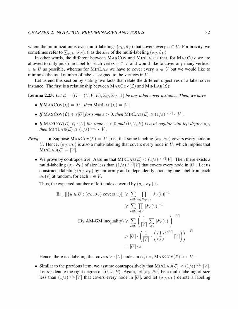
CHAPTER 2. NOTATION, PRELIMINARIES AND TOOLS 32
where the minimization is over multi-labelings (σU , σV ) that covers every u ∈ U . For brevity, wesometimes refer to
∑v∈V |σV (v)| as the size of the multi-labeling (σU , σV )
In other words, the different between MAXCOV and MINLAB is that, for MAXCOV we areallowed to only pick one label for each vertex v ∈ V and would like to cover any many verticesu ∈ U as possible, whereas for MINLAB we have to cover every u ∈ U but we would like tominimize the total number of labels assigned to the vertices in V .
Let us end this section by stating two facts that relate the different objectives of a label coverinstance. The first is a relationship between MAXCOV(L) and MINLAB(L):
Lemma 2.23. Let L = (G = (U, V,E),ΣU ,ΣV ,Π) be any label cover instance. Then, we have
• If MAXCOV(L) = |U |, then MINLAB(L) = |V |.
• If MAXCOV(L) 6 ε|U | for some ε > 0, then MINLAB(L) > (1/ε)1/|V | · |V |.
• If MAXCOV(L) 6 ε|U | for some ε > 0 and (U, V,E) is a bi-regular with left degree dU ,then MINLAB(L) > (1/ε)1/dU · |V |.
Proof. • Suppose MAXCOV(L) = |U |, i.e., that some labeling (σU , σV ) covers every node inU . Hence, (σU , σV ) is also a multi-labeling that covers every node in U , which implies thatMINLAB(L) = |V |.
• We prove by contrapositive. Assume that MINLAB(L) < (1/ε)1/|V ||V |. Then there exists amulti-labeling (σU , σV ) of size less than (1/ε)1/|V ||V | that covers every node in |U |. Let usconstruct a labeling (σU , σV ) by uniformly and independently choosing one label from eachσV (v) at random, for each v ∈ V .
Thus, the expected number of left nodes covered by (σU , σV ) is
EσV [|u ∈ U : (σU , σV ) covers u|] >∑u∈U
∏v∈NG(u)
|σV (v)|−1
>∑u∈U
∏v∈V|σV (v)|−1
(By AM-GM inequality) >∑u∈U
(1|V |
∑v∈V|σV (v)|
)−|V |
> |U | ·(
1|V |·((1
ε
)1/|V ||V |
))−|V |= |U | · ε
Hence, there is a labeling that covers > ε|U | nodes in U , i.e., MAXCOV(L) > ε|U |.
• Similar to the previous item, we assume contrapositively that MINLAB(L) < (1/ε)1/dU |V |.Let dV denote the right degree of (U, V,E). Again, let (σU , σV ) be a multi-labeling of sizeless than (1/ε)1/dU |V | that covers every node in |U |, and let (σU , σV ) denote a labeling
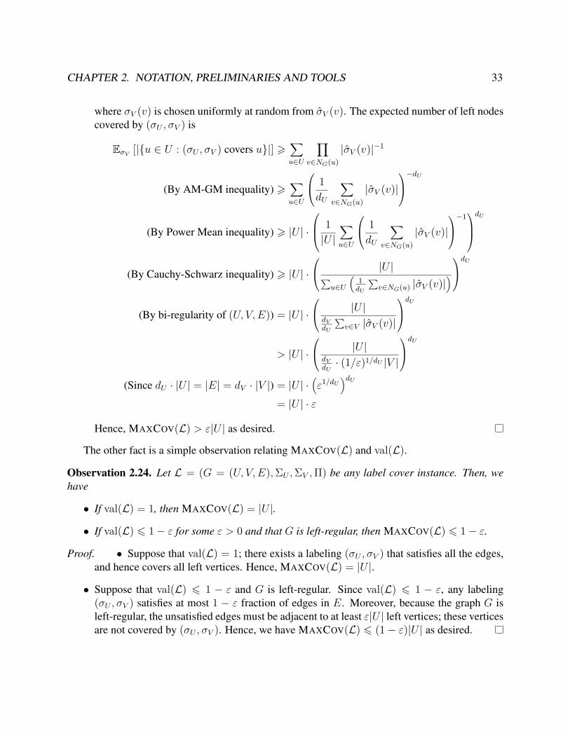
CHAPTER 2. NOTATION, PRELIMINARIES AND TOOLS 33
where σV (v) is chosen uniformly at random from σV (v). The expected number of left nodescovered by (σU , σV ) is
EσV [|u ∈ U : (σU , σV ) covers u|] >∑u∈U
∏v∈NG(u)
|σV (v)|−1
(By AM-GM inequality) >∑u∈U
1dU
∑v∈NG(u)
|σV (v)|−dU
(By Power Mean inequality) > |U | ·
1|U |
∑u∈U
1dU
∑v∈NG(u)
|σV (v)|−1
dU
(By Cauchy-Schwarz inequality) > |U | ·
|U |∑u∈U
(1dU
∑v∈NG(u) |σV (v)|
)dU
(By bi-regularity of (U, V,E)) = |U | · |U |
dVdU
∑v∈V |σV (v)|
dU
> |U | ·
|U |dVdU· (1/ε)1/dU |V |
dU
(Since dU · |U | = |E| = dV · |V |) = |U | ·(ε1/dU
)dU= |U | · ε
Hence, MAXCOV(L) > ε|U | as desired.
The other fact is a simple observation relating MAXCOV(L) and val(L).
Observation 2.24. Let L = (G = (U, V,E),ΣU ,ΣV ,Π) be any label cover instance. Then, wehave
• If val(L) = 1, then MAXCOV(L) = |U |.
• If val(L) 6 1− ε for some ε > 0 and that G is left-regular, then MAXCOV(L) 6 1− ε.
Proof. • Suppose that val(L) = 1; there exists a labeling (σU , σV ) that satisfies all the edges,and hence covers all left vertices. Hence, MAXCOV(L) = |U |.
• Suppose that val(L) 6 1 − ε and G is left-regular. Since val(L) 6 1 − ε, any labeling(σU , σV ) satisfies at most 1 − ε fraction of edges in E. Moreover, because the graph G isleft-regular, the unsatisfied edges must be adjacent to at least ε|U | left vertices; these verticesare not covered by (σU , σV ). Hence, we have MAXCOV(L) 6 (1− ε)|U | as desired.
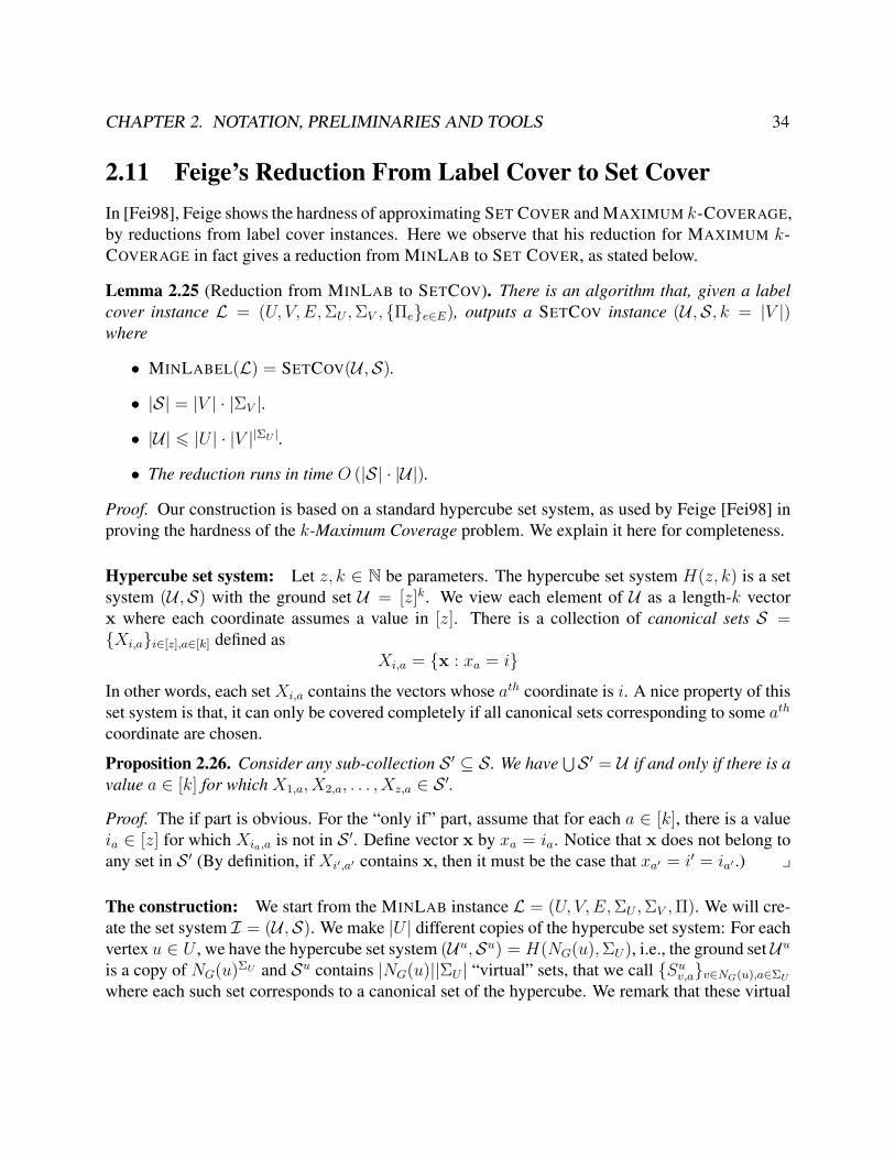
CHAPTER 2. NOTATION, PRELIMINARIES AND TOOLS 34
2.11 Feige’s Reduction From Label Cover to Set CoverIn [Fei98], Feige shows the hardness of approximating SET COVER and MAXIMUM k-COVERAGE,by reductions from label cover instances. Here we observe that his reduction for MAXIMUM k-COVERAGE in fact gives a reduction from MINLAB to SET COVER, as stated below.
Lemma 2.25 (Reduction from MINLAB to SETCOV). There is an algorithm that, given a labelcover instance L = (U, V,E,ΣU ,ΣV , Πee∈E), outputs a SETCOV instance (U ,S, k = |V |)where
• MINLABEL(L) = SETCOV(U ,S).
• |S| = |V | · |ΣV |.
• |U| 6 |U | · |V ||ΣU |.
• The reduction runs in time O (|S| · |U|).
Proof. Our construction is based on a standard hypercube set system, as used by Feige [Fei98] inproving the hardness of the k-Maximum Coverage problem. We explain it here for completeness.
Hypercube set system: Let z, k ∈ N be parameters. The hypercube set system H(z, k) is a setsystem (U ,S) with the ground set U = [z]k. We view each element of U as a length-k vectorx where each coordinate assumes a value in [z]. There is a collection of canonical sets S =Xi,ai∈[z],a∈[k] defined as
Xi,a = x : xa = i
In other words, each set Xi,a contains the vectors whose ath coordinate is i. A nice property of thisset system is that, it can only be covered completely if all canonical sets corresponding to some ath
coordinate are chosen.
Proposition 2.26. Consider any sub-collection S ′ ⊆ S. We have⋃S ′ = U if and only if there is a
value a ∈ [k] for which X1,a, X2,a, . . . , Xz,a ∈ S ′.
Proof. The if part is obvious. For the “only if” part, assume that for each a ∈ [k], there is a valueia ∈ [z] for which Xia,a is not in S ′. Define vector x by xa = ia. Notice that x does not belong toany set in S ′ (By definition, if Xi′,a′ contains x, then it must be the case that xa′ = i′ = ia′ .) y
The construction: We start from the MINLAB instance L = (U, V,E,ΣU ,ΣV ,Π). We will cre-ate the set system I = (U ,S). We make |U | different copies of the hypercube set system: For eachvertex u ∈ U , we have the hypercube set system (Uu,Su) = H(NG(u),ΣU), i.e., the ground set Uuis a copy of NG(u)ΣU and Su contains |NG(u)||ΣU | “virtual” sets, that we call Suv,av∈NG(u),a∈ΣUwhere each such set corresponds to a canonical set of the hypercube. We remark that these virtual
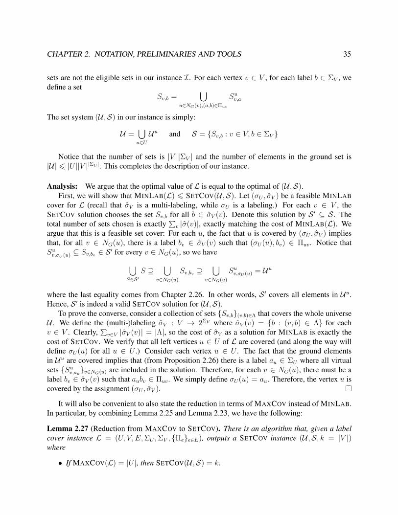
CHAPTER 2. NOTATION, PRELIMINARIES AND TOOLS 35
sets are not the eligible sets in our instance I. For each vertex v ∈ V , for each label b ∈ ΣV , wedefine a set
Sv,b =⋃
u∈NG(v),(a,b)∈ΠuvSuv,a
The set system (U ,S) in our instance is simply:
U =⋃u∈UUu and S = Sv,b : v ∈ V, b ∈ ΣV
Notice that the number of sets is |V ||ΣV | and the number of elements in the ground set is|U| 6 |U ||V ||ΣU |. This completes the description of our instance.
Analysis: We argue that the optimal value of L is equal to the optimal of (U ,S).First, we will show that MINLAB(L) 6 SETCOV(U ,S). Let (σU , σV ) be a feasible MINLAB
cover for L (recall that σV is a multi-labeling, while σU is a labeling.) For each v ∈ V , theSETCOV solution chooses the set Sv,b for all b ∈ σV (v). Denote this solution by S ′ ⊆ S. Thetotal number of sets chosen is exactly
∑v |σ(v)|, exactly matching the cost of MINLAB(L). We
argue that this is a feasible set cover: For each u, the fact that u is covered by (σU , σV ) impliesthat, for all v ∈ NG(u), there is a label bv ∈ σV (v) such that (σU(u), bv) ∈ Πuv. Notice thatSuv,σU (u) ⊆ Sv,bv ∈ S ′ for every v ∈ NG(u), so we have
⋃S∈S′
S ⊇⋃
v∈NG(u)Sv,bv ⊇
⋃v∈NG(u)
Suv,σU (u) = Uu
where the last equality comes from Chapter 2.26. In other words, S ′ covers all elements in Uu.Hence, S ′ is indeed a valid SETCOV solution for (U ,S).
To prove the converse, consider a collection of sets Sv,b(v,b)∈Λ that covers the whole universeU . We define the (multi-)labeling σV : V → 2ΣV where σV (v) = b : (v, b) ∈ Λ for eachv ∈ V . Clearly,
∑v∈V |σV (v)| = |Λ|, so the cost of σV as a solution for MINLAB is exactly the
cost of SETCOV. We verify that all left vertices u ∈ U of L are covered (and along the way willdefine σU(u) for all u ∈ U .) Consider each vertex u ∈ U . The fact that the ground elementsin Uu are covered implies that (from Proposition 2.26) there is a label au ∈ ΣU where all virtualsets Suv,auv∈NG(u) are included in the solution. Therefore, for each v ∈ NG(u), there must be alabel bv ∈ σV (v) such that aubv ∈ Πuv. We simply define σU(u) = au. Therefore, the vertex u iscovered by the assignment (σU , σV ).
It will also be convenient to also state the reduction in terms of MAXCOV instead of MINLAB.In particular, by combining Lemma 2.25 and Lemma 2.23, we have the following:
Lemma 2.27 (Reduction from MAXCOV to SETCOV). There is an algorithm that, given a labelcover instance L = (U, V,E,ΣU ,ΣV , Πee∈E), outputs a SETCOV instance (U ,S, k = |V |)where
• If MAXCOV(L) = |U |, then SETCOV(U ,S) = k.
CHAPTER 2. NOTATION, PRELIMINARIES AND TOOLS 36
• If MAXCOV(L) 6 ε · |U |, then SETCOV(U ,S) > (1/ε)1/k · k.
• |S| = |V | · |ΣV |.
• |U| 6 |U | · |V ||ΣU |.
• The reduction runs in time O (|S| · |U|).
Finally, we note that it is a well-known fact that we can reduce SETCOV to DOMSET byconstructing a graph whose vertices are U ∪S; there are edges between every pairs of subsets, andthere is an edge between S ∈ S to u ∈ U iff u belongs to S. It is obvious to see that the optimumof the DOMSET instance is exactly the same as that of the original SETCOV instance.

37
Part I
Problems Between P and NP
38
Chapter 3
A Birthday Repetition Theorem and ItsApplications
Polynomial-time reductions between computational problems are among the central tools in com-plexity theory. The rich and vast theory of hardness of approximation emerged out of the celebratedPCP Theorem [Aro+98; AS98] and the intricate web of polynomial-time reductions developed overthe past two decades. During this period, an extensive set of reduction techniques such as parallelrepetition and long-codes have been proposed and a variety of mathematical tools including dis-crete harmonic analysis, information theory and Gaussian isoperimetry have been applied towardsanalyzing these reductions. These developments have led to an almost complete understanding ofthe approximability of many fundamental combinatorial optimization problems like SET COVER
and MAX 3SAT. Yet, there are a few central problems such as computing approximate Nashequlibria, the DENSEST k-SUBGRAPH problem and the SMALL SET EXPANSION problem, thatremain out of reach of the web of polynomial-time reductions.
A promising new line of work proposes to understand the complexity of these problems throughthe lens of sub-exponential time reductions. Specifically, the idea is to construct a sub-exponentialtime reduction from 3SAT to the problem at hand, say, the Approximate Nash Equilibrium prob-lem. Assuming that 3SAT does not admit sub-exponential time algorithms (also known as theExponential Time Hypothesis (ETH) [IP01; IPZ01]), this would rule out polynomial time algo-rithms for the Approximate Nash Equilibrium problem.
At the heart of this line of works, lies the so-called birthday repetition of two-prover games.To elaborate on this, we begin by formally defining the notion of two-prover games1.
Definition 3.1. (Two-prover game) A two prover game G consists of
• A finite set of questions X, Y and corresponding answer sets ΣX ,ΣY .
• A distribution Q over pairs of questions X × Y .1The definition of two-prover games is in fact equivalent to that of Label Cover in Definition 2.3. However, for
the purpose of describing parallel and birthday repetitions, two-prover game interpretation is more natural.
CHAPTER 3. A BIRTHDAY REPETITION THEOREM AND ITS APPLICATIONS 39
• A verification function P : X × Y × ΣX × ΣY → 0, 1.
The value of the game is the maximum over all strategies φ : X ∪ Y → ΣX ∪ ΣY of the output ofthe verification function, i.e., val(G) = maxφ:X∪Y→ΣX∪ΣY E(x,y)∼Q[P (x, y, φ(x), φ(y))].
Two prover games earn their name from the following interpretation of the above definition:The game G is played between a verifier V and two cooperating provers Merlin1 and Merlin2who have agreed upon a common strategy, but cannot communicate with each other during thegame. The verifier samples two questions (x, y) ∼ Q and sends x to Merlin1 and y to Merlin2.The provers respond with answers φ(x) and φ(y), which the verifier accepts or rejects based on thevalue of the verifiaction function P (x, y, φ(x), φ(y)).
Two-prover games and, more specifically, a special class of two-prover games known as theLABEL COVER problem are the starting points for reductions in a large body of hardness of ap-proximation results. The PCP theorem implies that for some absolute constant ε0, approximatingthe value of a two prover game to within an additive ε0 is NP-hard. However, this hardness resulton its own is inadequate to construct reductions to other combinatorial optimization problems. Tothis end, this hardness result can be strengthened to imply that it is NP-hard to approximate thevalue of two-prover games to any constant factor, using the parallel repetition theorem.
For an integer k, the k-wise parallel repetition G⊗k of a game G can be described as follows.The question and answer sets in G⊗k consist of k-tuples of questions and answers from G. Thedistribution over questions in G⊗k is given by the product distribution Qk. The verifier for G⊗kaccepts the answers if and only if the verifier for G accepts each of the k individual answers.
Roughly speaking, the parallel repetition theorem asserts that the value of the repeated gameGk decays exponentially in k. Parallel repetition theorems form a key ingredient in obtainingtight hardness of approximation results, and have aptly received considerable attention in litera-ture [Raz98; Hol09; Rao11; DS14; Mos14; BG15].
Birthday repetition, introduced by Aaronson et al. [AIM14], is an alternate transformation ontwo-prover games defined as follows.
Definition 3.2. (Birthday Repetition) The (k × `)-birthday repetition of a two-prover game Gconsists of
• The set of questions in Gk×` are(Xk
)and
(Y`
)respectively, i.e., each question is a subset
S ⊆ X of size k and subset T ⊆ Y of size `.
• The distribution over questions is the uniform product distribution over(Xk
)×(Y`
).
• The verifier accepts only if, for every pair of (x, y) ∈ S × T such that (x, y) form a validpair of questions in G, i.e., (x, y) ∈ supp(Q), the answers to x and y are accepted in theoriginal game G.
The basic idea of birthday repetition can be traced back to the work of Aaronson et al. [Aar+09]on quantum multiprover proof systems QMA(k) for 3SAT. Subsequent work by Aaronson et al. [AIM14]
CHAPTER 3. A BIRTHDAY REPETITION THEOREM AND ITS APPLICATIONS 40
on the classical analogue of QMA(k), namely AM(k), formally defined birthday repetition fortwo-prover games, and set the stage for applications in hardness of approximation.
Unlike parallel repetition, birthday repetition is only effective for large values of k and `. Inparticular, if k, ` < o(
√|X|+ |Y |), then, for most pairs of S and T , there is no pair of questions
(x, y) ∈ S × T such that (x, y) belongs to the support of the questions in the original game.However, if we pick k = ` = ω(
√n) where n = |X| + |Y |, then by the birthday paradox,
with high probability the sets S, T contain an edge (x, y) from the original game G. Hence, forthis choice of k and `, the game played by the provers is seemingly at least as difficult to succeed,as the original game G. Aaronson et al. [AIM14] confirmed this intuition by proving the followingtheorem.
Theorem 3.3. [AIM14] For any two-prover game G such that Q is uniform over its support, if thebipartite graph induced by (X, Y, supp(Q)) is biregular, then val(Gk×`) 6 val(G) +O(
√nk`
).
On the one hand, birthday repetition is ineffective in that it has to incur a blowup of 2√n in the
size, to even simulate the original game G. The distinct advantage of birthday repetition is that theresulting game Gk,` has a distinct structure – in that it is a free game.
Definition 3.4. (Free game) A free game is a two-player game G = (X, Y,Q,ΣX ,ΣY , P ) suchthat Q is the uniform distribution over X × Y .
The birthday repetition theorem of Aaronson et al. [AIM14] immediately implies a hardnessof approximation for the value of free games. Specifically, they show that it is ETH-hard to ap-proximate free games to some constant ratio in almost quasi-polynomial time. Interestingly, thislower bound is nearly tight in that free games admit a quasipolynomial time approximation scheme(QPTAS) [Bar+11; AIM14].
Following Aaronson et al.’s work, birthday repetition has received numerous applications,which can be broadly classified in to two main themes. On the one hand, there are problems such ascomputing approximate Nash equilibria [BKW15; BPR16], approximating free games [AIM14],and approximate symmetric signaling in zero sum games [Rub17b], where the underlying prob-lems admit quasipolynomial-time algorithms [Dug14; LMM03; FS97] and birthday repetition canbe used to show that such a running time is necessary, assuming ETH. On the other hand, thereare computational problems like Densest k-Subgraph [Bra+17], injective tensor norms [Aar+09;HM13; Bar+12], 2-to-4-norms [Aar+09; HM13; Bar+12] wherein an NP-hardness of approxima-tion result seems out of reach of current techniques. But the framework of birthday repetition canbe employed to show a quasi-polynomial hardness assuming ETH2.
Unlike the parallel repetition theorem, the birthday repetition theorem of [AIM14] does notachieve any reduction in the value of the game. It is thus natural to ask whether birthday repetitioncan be used to decrease the value of a game, just like parallel repetition. Aaronson et al. conjecturednot only that the value of the game deteriorates with birthday repetition, but also that it decreases
2Although the hardness results for injective tensor norms and 2-to-4-norms build over quantum multiprover proofsystems, the basic idea of birthday repetition [Aar+09] lies at the heart of these reductions.
CHAPTER 3. A BIRTHDAY REPETITION THEOREM AND ITS APPLICATIONS 41
exponentially in Ω(k`/n). Notice that the expected number of edges between S and T in birthdayrepetition is Θ(k`/n).
The main technical contribution of this chapter is that we resolve the conjecture positively byshowing the following theorem.
Theorem 3.5. (Birthday Repetition Theorem (informal); See Theorem 3.15) Let G = (X, Y,Q,ΣX ,ΣY , P )be a two-prover game such that Q is uniform over its support, (X, Y, supp(Q)) is biregular. Ifval(G) 6 1− ε for some ε > 1/n, then
val(Gk×`) 6 (1− ε/2)Ω( k`n log(1/ε)).
Our theorem is, in fact, more general than stated above and can handle non-biregular graphs aswell as the case ε < 1/n, albeit with some loss in parameters (see Theorem 3.15).
We remark that Theorem 3.15 contains quantitative improvements over the corresponding the-orem in the conference version of this work [MR17a]. In particular, the birthday repetition theoremof [MR17a] has a factor of ε5 in the exponent instead of 1/ log(1/ε) in Theorem 3.15. To achievethis improvement, we use a completely different technique compared to that in [MR17a] based oncounting number of bicliques and Alon’s lemmas (Lemmas 2.14 and 2.15).
We also note that quantitatively Theorem 3.15 matches that of a follow-up work of Ko [Ko18],with an advantage that Theorem 3.15 applies to any two-prover games whereas Ko’s techniqueonly applies to projection games.
By definition, the birthday repetition theorem almost immediately implies a hardness of ap-proximation result for the value of a free game.
Corollary 3.6. Unless ETH is false, no polynomial time algorithm can approximate the value of afree game to within a factor of 2Ω(log(nq)) where n is the number of questions and q is the alphabet(answer set) size.
The above hardness result improves upon polylog(nq) ratio achieved in [AIM14] and is tightup to a factor of polyloglog(nq) in the exponent since there exists a polynomial-time algorithmthat achieves O(qε) approximation for every constant ε > 0 [AIM14; MM15].
Dense CSPsA free game can be considered an instance of 2-ary constraint satisfaction problems. From thisperspective, free games are dense, in that there are constraints between a constant fraction of allpairs of variables. As an application of our birthday repetition theorem, we will show almost-tighthardness of approximation results for dense CSPs. To this end, we begin by defining MAX k-CSPand its density.
Definition 3.7. (MAX k-CSP) A MAX k-CSP instance G consists of
• A finite set of variables V and a finite alphabet set Σ.
CHAPTER 3. A BIRTHDAY REPETITION THEOREM AND ITS APPLICATIONS 42
• A distribution Q over k-size subsets of variables(Vk
).
• A predicate P :(Vk
)× Σk → [0, 1].
The value of the instance is the maximum over all assignments φ : V → Σ of the expected outputof the predicate, i.e., val(G) = maxφ:V→Σ ES∼Q[P (S, φ|S)] where φ|S is the restriction of φ to S.
Finally, an instance is called ∆-dense if ∆ · Q(S) 6(|V |k
)for every S ∈
(Vk
). Fully-dense
instances are defined to be simply the 1-dense instances.
There has been a long line of works on approximating dense CSPs. Arora, Karger and Karpin-ski were first to devise a polynomial-time approximation scheme for the problem when alphabetsize is constant [AKK95]. Since then, numerous algorithms have been invented for approximat-ing dense CSPs; these algorithms use wide ranges of techniques such as combinatorial algorithmswith exhaustive sampling [AKK95; Veg+05; MS08; Yar14; MM15; FLP16], subsampling of in-stances [Alo+03; Bar+11], regularity lemmas [FK96; CCF10] and linear and semidefinite programhierarchies [VK07; BRS11; GS11; YZ14]. Among the known algorithms, the fastest is that ofYaroslavtsev [Yar14] that achieves approximation ratio (1 + ε) in qOk(log q/ε2) + (nq)O(1) time3
where n and q denote the number of variables and alphabet size respectively.Unfortunately, when q is (almost-)polynomial in n, none of the mentioned algorithms run in
polynomial time. CSPs in such regime of parameters have long been studied in hardness of approx-imation (e.g. [Bel+93; RS97; AS03; Din+11; MR10; Mos12]) and have recently received moreattention from the approximation algorithm standpoint, both in the general case [Pel07; CHK11;MM17] and the dense case [MM15]. The approximabilities of these two cases are vastly different.In the general case, it is known that, for some constant k > 0, approximating MAX k-CSP towithin a factor of 2log1−ε(nq) is NP-hard for any constant ε > 0 [Din+11]. Moreover, the long-standing Sliding Scale Conjecture of Bellare et al. [Bel+93] states there are constants k, ε > 0such that it is NP-hard to approximate MAX k-CSP to within a factor of (nq)ε. On the otherhand, aforementioned algorithms for dense CSPs rule out such hardnesses for the dense case.
While the gap between known approximation algorithms and inapproximability results in thegeneral case is tiny (2logε(nq) for any constant ε > 0), the story is different for the dense case, espe-cially when we restrict ourselves to polynomial-time algorithms. Aaronson et al.’s result only rulesout, assuming ETH, polylog(nq) factor approximation for such algorithms [AIM14]. However, fork > 2, no non-trivial polynomial time algorithm for dense MAX k-CSP on large alphabet is evenknown. We settle down the complexity of approximating dense MAX k-CSP almost completelyby answering the following fine-grained question: “for each i ∈ N, what is the best approximationfor dense MAX k-CSP, achievable by algorithms running in time (nq)i?”.
Manurangsi and Moshkovitz developed an algorithm for dense MAX 2-CSP that, when theinstance has value 1 − ε, can approximate the value to within a factor of O(q1/i/(1 − ε)i) in
3[Yar14] states that the algorithm takes qOk(1/ε2) + (nq)O(1) time but it in fact takes qOk(log q/ε2) + (nq)O(1)
time [Yar16].
CHAPTER 3. A BIRTHDAY REPETITION THEOREM AND ITS APPLICATIONS 43
(nq)O(i) time [MM15]4. Due to the algorithm’s combinatorial nature, it is unclear whether thealgorithm can be extended to handle dense MAX k-CSPs when k > 2.
Using a conditioning-based rounding technique developed in [BRS11; RT12; YZ14], we showthat the Sherali-Adams relaxation exhibits a similar approximation even when k > 2, as statedbelow.
Theorem 3.8. (Informal; See Theorem 3.29) For every i > 0 and any dense MAX k-CSP instanceof value 1−ε, anOk,ε(i/∆)-level of the Sherali-Adams relaxation yields anO(q1/i)-approximationfor the instance.
Using our birthday repetition theorem, we show that it is impossible to improve the abovetradeoff between run-time and approximation ratio using the sum-of-squares SDP hierarchy (akathe Lasserre SDP hierarchy). Specifically, we use birthday repetition on the Ω(n)-level Lasserreintegrality gap for MAX 3XOR by Schoenebeck [Sch08] to show the following.
Lemma 3.9. (Informal; See Lemma 3.23) For every sufficiently large i > 0, there is a fully-denseMAX 2-CSP instance of value 1/(nq)1/i such that the value of Ω(i)-level Lasserre relaxation isone.
Instead, if we assume that there exists a constant ε > 0 so that MAX 3SAT cannot be ap-proximated to 1 − ε in sub-exponential time (which we call the Exponential Time Hypothesis forApproximating MAX 3SAT (Gap-ETH)), then we can arrive at the following hardness result.
Lemma 3.10. (Informal; See Lemma 3.22) Assuming Gap-ETH, for every sufficiently large i > 0,no (nq)O(i)-time algorithm can approximate fully-dense MAX 2-CSP to within a factor of (nq)1/i.
Thus, assuming Gap-ETH, our hardness result and algorithm resolve complexity of approx-imating dense CSPs up to a factor of polylog(i) and a dependency on k in the exponent of therunning time.
Almost Optimal AM(2) Protocol for 3SATAnother interpretation of our improved hardness of approximation of free games is as an improvedAM(2) protocol for 3SAT. The Arthur-Merlin (AM) protocol [Bab85] is a protocol where Arthur(verifier) tosses some random coins and sends the results to Merlin (prover). The prover sends backa proof to Arthur who then decides whether to accept it. Motivated by quantum complexity classQMA(k), Aaronson et al. [AIM14] proposes a multi-prover version of AM called AM(k) wherethere are k non-communicating Merlins5. Authur sends an independent random challenge to eachMerlin who then sends an answer back to Arthur. Finally, Arthur decides to accept or reject basedon the received answers. The protocol is formally defined below.
4Note that it is unclear whether Aaronson, Impagliazzo and Moshkovitz’s algorithm [AIM14] that achieves asimilar guarantee for free games can be extended to handle dense MAX 2-CSP.
5AM(k) is not to be confused with AM[k] defined in [Bab85]. In AM[k], there is only one Merlin but Arthur andMerlin are allowed to engage in k rounds of communication.
CHAPTER 3. A BIRTHDAY REPETITION THEOREM AND ITS APPLICATIONS 44
Definition 3.11. [AIM14] An AM(k) protocol for a language L ⊆ 0, 1∗ of length p(n) = kq(n),completeness c(n), and soundness s(n) consists of a probabilistic polynomial-time verifier V suchthat
• (Completeness) For every x ∈ L, there exists functions m1, . . . ,mk : 0, 1q(n) → 0, 1q(n)
such that Pry1,...,yk∼0,1q(n) [V (x, y1, . . . , yk,m(y1), . . . ,m(yk))] > c(n), and,
• (Soundness) For every x /∈ L and for every function m1, . . . ,mk : 0, 1q(n) → 0, 1q(n),we have Pry1,...,yk∼0,1q(n) [V (x, y1, . . . , yk,m(y1), . . . ,m(yk))] 6 s(n)
The complexity class AMp(n)(k) is a set of all languages L such that there exists an AM(k)protocol of length p(n), completeness 1/3, and soundness 2/3. Finally, the class AM(k) is definedas⋃c∈N AMnc(k).
Similar to the interpretation of a two-prover game as a two-prover protocol, a free game canbe viewed as an AM(2) protocol. Under this view, inapproximabilities of free games translate toAM(2) protocols whereas approximation algorithms for free games translate to lower bounds onthe lengths of AM(2) protocols.
With this viewpoint, Aaronson et al. constructed, via birthday repetition, an AM(2) protocol oflength n1/2+o(1)poly(1/δ) for 3SAT with completeness 1 and soundness δ for every δ > 0. Theyalso showed a lower bound of Ω(
√n log(1/δ)) on the length of such protocol. Equipped with our
birthday repetition theorem, we construct an AM(2) protocol whose length is optimal up to a factorof polylogn.
Lemma 3.12. For any δ > 0, there is an AM(2) protocol for 3SAT of length O(√n log(1/δ)) with
completeness 1 and soundness δ.
We note that, by picking δ = 1/3, Lemma 3.12 immediately imply 3SAT ∈ AMO(√n)(2).
Since every problem in NTIME(n) is reducible to a quasi-linear size 3SAT instance [Coo88],we arrive at the following corollary, resolving the first open question posted in [AIM14].
Corollary 3.13. NTIME(n) ⊆ AMO(√n)(2).
Organization of this chapterThe rest of the chapter is organized as follows. In the following section, we provide preliminariesand state notations that we use in this chapter. Then, in Section 3.2, we prove our main theorems.Next, Section 3.3 demonstrates applications of our birthday repetition theorem, including newhardnesses of approximation and Lasserre integrality gap for dense CSPs, and an almost optimalAM(2) protocol for 3SAT. The algorithm for dense MAX k-CSP is described and its approxima-tion guarantee is proved in Section 3.4. Finally, we conclude by proposing open questions andfuture research directions in Section 3.5.
CHAPTER 3. A BIRTHDAY REPETITION THEOREM AND ITS APPLICATIONS 45
3.1 Additional Preliminaries and NotationsIn this section, we define notations and state some well-known facts that will be subsequently used.
3.1.1 Information TheoryLet us define some information theoretic notions that will be useful in the analysis of our algo-rithm. The informational divergence (aka Kullback-Leibler divergence) between two probabil-ity distributions X and Y is DKL(X‖Y) = ∑
θ∈supp(X )X (θ) log(X (θ)/Y(θ)). Note that, whensupp(Y) 6⊆ supp(X ), we let DKL(X‖Y) = ∞. It is well-known that DKL(X‖Y) > 0 for anydistributions X and Y .
The entropy of a random variable x ∼ X is defined as H(x) = −∑θ∈supp(X )X (θ) logX (θ).For jointly distributed random variables x1, . . . , xn, the entropy of x1, . . . , xn is defined similarlyas H(x1, . . . , xn) = −∑(θ1,...,θn)∈supp(X1,...,n)X1,...,n(θ) logX1,...,n(θ) where X1,...,n is the joint dis-tribution of x1, . . . , xn.
The conditional entropy H(x1, . . . , xn−1|xn) is defined as Eθ∼supp(Xn)[H(x1, . . . , xn−1)|xn =θ] where Xn is the marginal distribution of xn.
Last information theoretic measure we will use is the total correlation defined asC(x1; . . . ;xn) =DKL(X1,...,n‖X1×· · ·×Xn) whereX1,...,n is the joint distribution of x1, . . . , xn whereasX1, . . . ,Xnare the marginal distributions of x1, . . . , xn respectively. We note that the total correlation definedhere is always non-negative whereas the mutual information can be negative.
The total correlation is related to entropies and mutual information as follows.
Lemma 3.14. For any random variables x1, . . . , xn,C(x1; . . . ;xn) = ∑i∈[n] H(xi)−H(x1; . . . ;xn).
Finally, similar to conditional entropy and conditional mutual information, we define the con-ditional total correlation as C(x1; . . . ;xn−1|xn) = Eθ∼supp(Xn)[C(x1; . . . ;xn−1)|xn = θ].
3.1.2 Two-prover Game, Free Game and MAX k-CSPTwo-prover games, free games, and MAX k-CSP are defined in similar manners as in the intro-duction. However, for convenience, we write the predicates as PS(φ|S) instead of P (S, φ|S), and,whenQ is the uniform distribution on Θ, we sometimes write the instance as (V,Θ, PS) insteadof (V,Q, PS). Moreover, for an assignment φ of a MAX k-CSP instance G = (V,W , PS),we define its value as valG(φ) = ES∼W [PS(φ|S)]. When it is clear from the context, we will dropG and write it simply as val(φ). Note that val(G) is the maximum of valG(φ) among all possibleassignments φ’s. We say that G is satisfiable if its value is one.
We use n to denote the number of variables |V |, q to denote the alphabet size |Σ| and Nto denote the instance size | supp(W)|qk, the number of bits needed to encode the input if eachpredicate is a boolean function. Note that, when the instance is fully dense, N is simply (nq)k.Similar notations are also used for two-prover games and free games.
CHAPTER 3. A BIRTHDAY REPETITION THEOREM AND ITS APPLICATIONS 46
3.1.3 Sherali-Adams and Lasserre HierarchiesWe also consider two hierarchies of linear and semidefinite program relaxations of MAX k-CSP.For compactness, we only write down the relaxations of MAX k-CSP but do not describe thehierarchies in full details. For interested readers, we refer to Chlamtác and Tulsiani’s survey on thetopic [CT12].
The first hierarchy we consider is the Sherali-Adams (SA) hierarchy, introduced in [SA90]. Anr-level SA solution of a MAX k-CSP instance G = (V,W , PS) is a collection µ = XS|S|6tof distributions XS on ΣS for every subset S of V of size at most r such that, for every S, T ⊆ Vof size at most r, the marginal probability of XS and XT on ΣS∩T agrees. The value of an r-levelSA solution µ for r > k is defined to be valSA(µ) = ES∼W [ExS∼µ[PS(xS)]] where ExS∼µ[PS(xS)]is a shorthand for EφS∼Xi1,...,ik [PS(φS)] when S = (xi1 , . . . , xik). The optimal of the r-level SArelaxation of G, optrSA(G), is defined as the maximum value among all the r-level SA solutions. Itis easy to see that finding optrSA(G) can be formulated as a linear program with at most (nq)O(r)
variables and inequalities and, thus, can be solved in (nq)O(r) time.Another hierarchy we consider is the Lasserre hierarchy [Las00]. Before stating the Lasserre
relaxation for MAX k-CSP, we define additional notations regarding assignments. Two assign-ments φ1 ∈ ΣS1 , φ2 ∈ ΣS2 are said to be consistent if φ1(x) = φ2(x) for all x ∈ S1 ∩ S2. The twoassignments are said to be inconsistent otherwise. More than two assignments are consistent if ev-ery pair of the assignments is consistent; otherwise, they are said to be inconsistent. Moreover, fortwo consistent assignments φ1 ∈ ΣS1 , φ2 ∈ ΣS2 , we define φ1φ2 ∈ ΣS1∩S2 by φ1φ2(x) = φ1(x)if x ∈ S1 and φ1 φ2(x) = φ2(x) otherwise.
An r-level Lasserre solution of an instance G = (V,W , PS) is a collection U(S,φS)|S|6r,φS∈ΣS
of vectors U(S,φS) for all S ⊆ V of size at most r and assignments φS of S satisfying the followingconstraints.
〈U(S1,φ1), U(S2,φ2)〉 > 0 ∀S1, S2, φ1φ2
〈U(S1,φ1), U(S2,φ2)〉 = 〈U(S3,φ3), U(S4,φ4)〉 ∀S1 ∪ S2 = S3 ∪ S4 and φ1 φ2 = φ3 φ4
〈U(S1,φ1), U(S2,φ2)〉 = 0 ∀S1, S2, φ1φ2 s.t. φ1, φ2 are inconsistent∑σ∈Σ‖U(x,σ)‖2 = 1 ∀x ∈ V
‖U(∅,∅)‖ = 1
where S1, S2, S3, S4 are over all subset of V of size at most r and φ1, φ2, φ3, φ4 are over all assign-ments of S1, S2, S3, S4 respectively. The value of an r-level Lasserre solution U(S,φS) is definedas valLas(U(S,φS)) = ES∼W [∑φS∈ΣS ‖U(S,φS)‖2PS(φS)]. A Lasserre solution is called completeif its value is one.
Note that we abuse the notation here as S in U(S,φS) is a set whereas S inW is a tuple. Hereand elsewhere in this chapter, when we write U(S,φS) for some tuple S = (xi1 , . . . , xim), this simplyrefers to Uxi1 ,...,xim,φS if the assignment φS does not assign the same variable to different valuesand the all zero vector otherwise. Finally, we use optrLas(G) to denote the maximum value amongall r-level Lasserre solutions U(S,φS).
CHAPTER 3. A BIRTHDAY REPETITION THEOREM AND ITS APPLICATIONS 47
It is not hard to see that finding optrLas(G) can be formulated as SDP with (nq)O(r) variablesand, hence, can be approximated up to arbitrarily small error within (nq)O(r) time. Moreover, itis known that the r-level Lasserre relaxation is stronger than the r-level SA relaxation [Lau03].In the case of MAX k-CSP, this can be easily seen since we can define an r-level SA solutionµ = XS|S|6t from an r-level Lasserre solution U(S,φS) by XS(φS) = ‖U(S,φS)‖2.
3.2 Birthday Repetition Theorem and Its ProofIn this section, we prove our birthday repetition theorem, stated formally below.
Theorem 3.15. Let G = (X, Y,E,ΣX ,ΣY , P(x,y)) be any two-prover game. Suppose furtherthat (X, Y,E) is τ -almost-biregular. If val(G) = 1− ε, then for all 0 6 k 6 |X|, 0 6 ` 6 |Y |, wehave
val(Gk×`) 6(
1− ε
2τ
)Ω( k`log(τ/ε)(n+τ/ε))
.
To prove Theorem 3.15, we have to show that any strategy ψ of Gk×` is accepted with prob-
ability at most(1− ε
2τ
)Ω( k`log(τ/ε)(n+τ/ε)). Equivalently, we would like to show that the graph
GSATψ :=
((Xk
),(Y`
), ESAT
ψ
), where ESAT
ψ denote the set of all accepted pairs of questions, is sparse.Let us recall Alon’s lemmas (Lemmas 2.14 and 2.15), which roughly states that, if a graph
contains few labelled copies of biclique Ks,t, then it must be sparse. Hence, to show that GSATψ is
sparse, it suffices to bound the number of labelled copies of Ks,t in GSATψ for appropriately chosen
s, t (which will be specified later), and invoke Alon’s lemmas. To do so, we first define additionalnotations.
• Let AX :(Xk
)s→ P(X) denote a “flattening” operation that, on input L ∈
(Xk
)s, outputs
the sets of all elements that appears in at least one of the sets in L; more formally,AX(L) :=∪u∈Lu. We define AY :
(Y`
)t→P(Y ) similarly by AY (R) := ∪v∈Rv.
• Let Ks,t denote the set of labelled copies of Ks,t in the graph GSATψ , i.e.,
Ks,t :=
(L,R) ∈(Xk
)s×(Y`
)t∣∣∣ ∀u ∈ L, ∀v ∈ R, u 6= v ∧ (u, v) ∈ ESATψ
.
• For every A ⊆ X,B ⊆ Y , letK⊆s,t(A,B) denote the set of labelled copies of Ks,t whose flat-tenings are contained inA,B, i.e.,K⊆s,t(A,B) := (L,R) ∈ Ks,t | AX(L) ⊆ A ∧ AY (R) ⊆ B.We remark here that Ks,t is equal to Ks,t(X, Y ).
Now, the birthday repetition theorem can be proved via two simple observations. The firstobservation is that, any labelled copy (L,R) of Ks,t cannot have flattenings that are both large.This is because (L,R) in fact induces a (partial) strategy for the original game that is acceptedfor all edges whose endpoints are in AX(L) and AY (R). Hence, if both AX(L) and AY (R) are
CHAPTER 3. A BIRTHDAY REPETITION THEOREM AND ITS APPLICATIONS 48
already large, then this strategy would violate the assumption that val(G) = 1− ε. A more preciseversion of the statement is proved below.
Observation 3.16. Let (L,R) ∈(Xk
)s×(Y`
)tbe any labelled Ks,t of GSAT
ψ . Then, |AX(L)| 6(1− ε
2τ
)|X| or |AY (R)| 6
(1− ε
2τ
)|Y |.
Proof. Suppose for the sake of contradiction that there exists a labelled Ks,t copy (L,R) of GSATψ
such that |AX(L)| >(1− ε
2τ
)|X| and |AY (R)| >
(1− ε
2τ
)|Y |. Let f : AX(L) ∪ AY (R) →
ΣX ∪ ΣY be a partial strategy to G defined as follows.
• For every x ∈ AX(L), let f(x) = ψ(u)x for u ∈ L that contains x (when there are multiplesuch u’s, pick one arbitrarily).
• Similarly, for every y ∈ AY (R), let f(y) = ψ(v)y for v ∈ R that contains x.
Consider any edge (x, y) ∈ E ∩ (AX(L)×AY (R)). Let u ∈ L, v ∈ R be such that x ∈ u, y ∈v, f(x) = ψ(u)x and f(y) = ψ(v)y. Since u ∈ L, v ∈ R and (L,R) is a labelled copy of a bicliqueof GSAT
ψ , we must have (u, v) ∈ ESATψ ; equivalently, (ψ(u), ψ(v)) is an accepting answer of the
birthday repetition game for the edge (u, v). This implies that the verifier of the original game Gaccepts (ψ(u)x, ψ(v)y) = (f(x), f(y)) for the edge (x, y).
As a result, the verifier of the original game G accepts all edges in E ∩ (AX(L)×AY (R)) forpartial strategy f . In other words, the number of edges it does not accept is at most
∑x/∈AX(L)
degG(x) +∑
y/∈AY (R)degG(y) 6
∑x/∈AX(L)
(τ · min
x′∈XdegG(x′)
)+
∑y/∈AY (R)
(τ ·min
y′∈YdegG(y′)
)
6 τ |E| ·(|X| − |AX(L)|
|X|
)+ τ |E| ·
(|Y | − |AY (R)|
|Y |
)< ε|E|,
where the first inequality comes from the τ -almost-biregularity of G and the last inequality comesfrom our assumptions on the size ofAX(L),AY (R). This contradicts the assumption that val(G) =1− ε, which concludes our proof.
Another observation is that, if we fix A ⊆ X,B ⊆ Y such that either A or B is small and countthe number of labelled copies of Ks,t whose flattenings are contained in A,B (i.e. |Ks,t(A,B)|),then this number will be much smaller than
(|X|k
)s(|Y |`
)t. Intuitively, this is just because we must
choose every left vertex from(Ak
)instead of
(Xk
)and every right vertex from
(B`
)instead of
(Y`
).
This is formalized below.
Observation 3.17. For everyA ⊆ X,B ⊆ Y , we have |K⊆s,t(A,B)| 6(|A||X|
)sk ( |B||Y |
)t` (|X|k
)s(|Y |`
)t.
CHAPTER 3. A BIRTHDAY REPETITION THEOREM AND ITS APPLICATIONS 49
Proof. Consider any (L,R) ∈ K⊆s,t(A,B). SinceAX(L) ⊆ A andAY (R) ⊆ B, we have L ∈(Ak
)sand R ∈
(B`
)t. This implies that K⊆s,t(A,B) ⊆
(Ak
)s×(B`
)t. Hence,
|K⊆s,t(A,B)| 6(|A|k
)s(|B|`
)t6
(|A||X|
)sk ( |B||Y |
)t` (|X|k
)s(|Y |`
)t,
as desired.
With these two observations ready, the proof of the birthday repetition theorem is straightfor-ward: we simply sum the bounds in Observation 3.17 over an appropriate range of (A,B) whichis given by Observation 3.16.
Proof of Theorem 3.15. Let m = 100(n + τ/ε) log(100τ/ε). Pick s := dm/ke and t := dm/`e.From Observation 3.16, we have
Ks,t ⊆
⋃A⊆X,|A|=b(1− ε
2τ )|X|cK⊆s,t(A, Y )
∪ ⋃B⊆Y,|B|=b(1− ε
2τ )|Y |cK⊆s,t(X,B)
. (3.1)
As a result, we can bound |Ks,t| by
|Ks,t| 6
∑A⊆X,|A|=b(1− ε
2τ )|X|c|K⊆s,t(A, Y )|
+
∑B⊆Y,|B|=b(1− ε
2τ )|Y |c|K⊆s,t(X,B)|
(Observation 3.17) 6
∑A⊆X,|A|=b(1− ε
2τ )|X|c
(1− ε
2τ
)sk (|X|k
)s(|Y |`
)t+
∑B⊆Y,|B|=b(1− ε
2τ )|Y |c
(1− ε
2τ
)t` (|X|k
)s(|Y |`
)t=((|X|d ε|X|2τ e
)(1− ε
2τ
)sk+(|Y |d ε|Y |2τ e
)(1− ε
2τ
)t`)(|X|k
)s(|Y |`
)t
(From our choice of s, t) 6((|X|d ε|X|2τ e
)+(|Y |d ε|Y |2τ e
))(1− ε
2τ
)m (|X|k
)s(|Y |`
)t
6(
(2eτ/ε)dε|X|2τ e + (2eτ/ε)d
ε|Y |2τ e
)(1− ε
2τ
)m (|X|k
)s(|Y |`
)t
6 (2eτ/ε)2+ εn2τ
(1− ε
2τ
)m (|X|k
)s(|Y |`
)t
(From our choice of m) 6 20.1mε/τ(
1− ε
2τ
)m (|X|k
)s(|Y |`
)t
CHAPTER 3. A BIRTHDAY REPETITION THEOREM AND ITS APPLICATIONS 50
6(
1− ε
2τ
)0.5m(|X|k
)s(|Y |`
)t.
Now, Lemma 2.15 implies that
|ESATψ | 6
((1− ε
2τ
)0.5m)1/(st) (|X|
k
)(|Y |`
)=(
1− ε
2τ
)Ω( k`log(τ/ε)(n+τ/ε))
(|X|k
)(|Y |`
).
In other words, every strategy ψ is accepted with probability at most(1− ε
2τ
)Ω( k`log(τ/ε)(n+τ/ε)).
Hence, we have val(Gk×`) 6(1− ε
2τ
)Ω( k`log(τ/ε)(n+τ/ε)) as desired.
3.3 Applications of the Birthday Repetition TheoremWe next provide several implications of our birthday repetition theorem, including hardness ofapproximation results and integrality gaps for dense CSPs and improved AM(2) protocol for 3SAT.
3.3.1 Lower Bounds for Fully-Dense CSPsWe start with inapproximability and integrality gaps for fully dense MAX 2-CSP. Note that thesebounds also carry over to fully dense MAX k-CSP for any k > 2, since we can always constructan instance of the latter from the former by making each predicate ignore the last k − 2 variables.
As the birthday repetition theorem is stated in terms of free games, it will be convenient to firstshow the connection from free games to dense CSPs. Specifically, given a free games, one caneasily creates a “symmetrized” version of the game that is a fully-dense MAX 2-CSP and has thesame value of the original game:
Lemma 3.18 (Symmetrization of Free Games). Given a free game G = (X, Y,ΣX ,ΣY , P ), wecan, in polynomial time, create a MAX 2-CSP instance Gsym with alphabet ΣX × ΣY such that (i)val(Gsym) 6 val(G) and (ii) if val(G) = 1, then val(Gsym) = 1.
Proof. We define an instance Gsym = (X × Y,ΣX × ΣY , P′) where the variables are X × Y , the
alphabet is ΣX × ΣY and P ′(x1,y1),(x2,y2)((σx1 , σy1), (σx2 , σy2)) = ∏i,j∈1,2 P(xi,yj)(σxi , σyj).
Now, we will show that val(Gsym) 6 val(G). Let φ be an optimal assignment of Gsym, i.e.,where val(φ) = val(Gsym). Let f be a strategy for G defined randomly as follows: for everyx ∈ X , randomly select y ∈ Y and set f(x) = φ(x, y)1, and, for every y ∈ Y , randomly selectx ∈ X and set f(x) = φ(x, y)2. We have
Ef [val(f)] = Ef,(x,y)∼(X×Y )[P(x,y)(f(x), f(y))]= E(x,y),(x′,y′)∼(X×Y )[P(x,y)(φ((x, y′))1, φ((x′, y))2)]
= 1|X||Y |
E(x,y)∼(X×Y )[P(x,y)(φ(x, y)1, φ(x, y)2)]+
CHAPTER 3. A BIRTHDAY REPETITION THEOREM AND ITS APPLICATIONS 51
(1− 1|X||Y |
)E(x,y),(x′,y′)∼(X×Y )[P(x,y)(φ(x, y′)1, φ(x′, y)2) | (x, y) 6= (x′, y′)] (3.2)
We can bound the first term by
E(x,y)∼(X×Y )[P(x,y)(φ(x, y)1, φ(x, y)2)]= E(x,y),(x′,y′)∼(X×Y )[P(x,y)(φ(x, y)1, φ(x, y)2) | (x′, y′) 6= (x, y)]6 E(x,y),(x′,y′)∼(X×Y )[P ′(x,y),(x′,y′)(φ(x, y), φ(x′, y′)) | (x′, y′) 6= (x, y)]= val(φ).
The second term can be bounded similarly:
E(x,y),(x′,y′)∼(X×Y )[P(x,y)(φ(x, y′)1, φ(x′, y)2) | (x, y) 6= (x′, y′)]6 E(x,y),(x′,y′)∼(X×Y )[P ′(x′,y),(x,y′)(φ(x′, y), φ(x, y′)) | (x, y) 6= (x′, y′)]= val(φ).
Plugging both back to (3.2), we get Ef [val(f)] > val(φ). Hence, we have val(G) > val(φ) =val(Gsym), concluding the first part of the claim.
Finally, suppose that val(G) = 1; let f be an optimal strategy for G. The let φ be the assignmentof Gsym defined by φ(x, y) := (f(x), f(y)). It is obvious that φ satisfies all constraints.
ETH-Based Hardness of Approximation of Fully-Dense MAX 2-CSP
The first application of the birthday repetition theorem we present is an ETH-based almost-polynomialratio hardness for fully-dense MAX k-CSP, as stated formally below.
Lemma 3.19. Assuming ETH, for any k > 2, no polynomial-time algorithm can, given any fully-dense MAX k-CSP instance G of size N , distinguish val(G) = 1 from val(G) 6 2−Ω(logN).
We prove this by essentially applying the birthday repetition theorem with k = ` = Ω(n) toa two-prover game produced by Dinur’s PCP Theorem [Din07] (Theorem 2.2). Note, however,that Theorem 2.2 produces a Gap-3SAT instance instead of a two-prover game. Nevertheless,reductions between the two are standard. Here we use the so-called clause/variable reduction.This reduction is well-known and has appeared in literatures before (in e.g. [AIM14]). It is statedformally below.
Definition 3.20. (Clause/variable game) For any MAX k-CSP instance G = (V,E, PS), itsclause/variable game is a projection game G ′ = (X ′, Y ′,Σ′X ,Σ′Y , E ′, P ′(x,y)) defined as follows.X ′ is the set of constraints of G, i.e., X ′ = E. Y ′ is V , the set of variables of G. Σ′X is Σk; for eachconstraint S, Σ′X is identified with the assignments of S in G. Σ′Y is simply Σ. Finally, E ′ containsall (S, x) such that x ∈ S and P(S,x)(φ, σ) = 1 iff PS(φ) = 1 and φ(x) = σ.
It is easy to see that, when val(G) is bounded away from one, then so is val(G ′):
CHAPTER 3. A BIRTHDAY REPETITION THEOREM AND ITS APPLICATIONS 52
Proposition 3.21. Let G and G ′ be as in Definition 3.20. If val(G) 6 1−ε, then val(G ′) 6 1−ε/k.
Proof. Suppose for contrapositively that there is an assignment φ′ of G ′ with val(φ′) > 1 − ε/k.Define φ : V → Σ by φ(x) := φ′(x) for every x ∈ V . Since less than ε/k fraction of the edges arenot satisfied by φ′ in G ′ and each S ∈ X ′ has degree k, more than 1− ε fraction of S ∈ X ′ touchesonly satisfied edges. These clauses are satisfied by φ in G. Hence, val(φ) > 1− ε.
We can now prove Lemma 3.19.
Proof of Lemma 3.19. Given 3SAT instance φ of m clauses. We first use Dinur’s PCP Theorem(Theorem 2.2) to reduce φ to φ′ with m′ = m logcm clauses. Let G be the clause-variable gameof φ′. Consider the fully-dense MAX 2-CSP instance Gk×`sym which is the symmetrization of the(k × `)-birthday repetition game, where k = ` = m/ log2m.
Let n and q be the number of variables and the alphabet size of Gk×`sym . We have n 6(m′
k
)26
2(m′)2k 6 2O( mlogm) and q 6 2O(k) 6 2O( m
logm). Hence, the size of Gk×`sym is N = (nq)O(1) 62O(m/ logm). We next analyze the completeness and soundness of the reduction.
When val(φ) = 1, from the PCP theorem, we have val(φ′) = 1. It is also obvious from thereduction that val(Gk×`sym ) is one. On the other hand, when val(φ) < 1, we have val(φ′) 6 1 − ε,meaning that val(G) 6 1− ε/3. Hence, by Theorem 3.15 and Lemma 3.18, we have
val(Gk×`sym ) 6 (1− Ω(ε))Ω(k2m′2
)6 2−Ω(m) = 2−Ω(log N).
Thus, if a algorithm can distinguish val(Gk×`sym ) = 1 from val(Gk×`sym ) 6 2−Ω(log N) in time poly-nomial in N , then it can also solve 3SAT in time 2O(n/ logn) time, violating ETH.
Improved Hardness of Approximation Result Based on Gap-ETH
The polyloglogN loss in the exponent of Lemma 3.19 is due to the quasi-linear size of the PCPand can be eliminated if we instead assume the stronger Gap-ETH:
Lemma 3.22. Assuming Gap-ETH, for any sufficiently large i, no algorithm can, given any fully-dense MAX 2-CSP G of size N , distinguish val(G) = 1 from val(G) 6 N−1/i in time N O(i).
The proof is essentially the same as that of Lemma 3.19 except that, since the size of our startinggame is linear, we can now use birthday repetition for k = ` = Θi(n) instead of n/polylog(n).
Proof of Lemma 3.22. Given Gap-3SAT instance φ of m variables. Let G be its clause/variablegame. Observe that G has m′ = O(m) variables, O(1) alphabet size and maximum degree O(1).Consider Gk×`sym , the symmetrized (k×`)-birthday repetition with k = ` = βn log i
iwhere β is a small
constant which to be chosen later.
CHAPTER 3. A BIRTHDAY REPETITION THEOREM AND ITS APPLICATIONS 53
Let n and q be the number of variables and the alphabet size of Gk×`sym . We have q 6 2O(k) 6
2O(βn log ii ). Moreover, when β is sufficiently small, we have
n 6
(m′
k
)2
6
(em′
k
)2k
=(O
(i
β log i
))2l
6 2O(βm log2 i log(1/β)
i
)6 2O
(√βm log2 i
i
).
As for the completeness and soundness of the reduction, first, it is obvious that val(φ) = 1implies val(Gk×`sym ) = 1. Otherwise, from Proposition 3.21, if val(φ) 6 1−ε, then val(G) 6 1−ε/3.By by Theorem 3.15 and Lemma 3.18, we have
val(Gk×`sym ) 6 (1− Ω(ε))Ω(k2m′
)6 2−Ω(β2n log2 i/i2) 6 (nq)−Ω(β2/i) = N−Ω(β2/i)
where N = (nq)O(1) 6 2O(√βn log2 i/i) is the size of Gk×`sym .
Pick β to be sufficiently small so that N 6 O(2δm log2 i/i) where δ is the constant from Gap-ETH. If an algorithm distinguishes val(Gk×`sym ) = 1 from val(Gk×`sym ) 6 (N)−Ω(1/i) inO(N
ilog2 i ) time,
it also distinguishes val(φ) = 1 from val(φ) 6 1− ε in time O(2δm), violating Gap-ETH.
Lasserre Integrality Gap for Fully-Dense MAX 2-CSP
We will now show how to get a polynomial integrality gap for the Lasserre relaxation for denseCSPs. In particular, even for Ω(i)-level of Lasserre hierarchy, the integrality gap remains N1/i forfully-dense MAX 2-CSP, as stated formally below.
Lemma 3.23. For any sufficiently large N and any sufficiently large i, there exists a fully-dense
MAX 2-CSP instance G of size N such that optΩ(i)Las (G) = 1 and val(G) 6 N−1/i.
One way to interpret Lemma 3.23 is as a lower bound for SDP or LP hierarchies algorithmfor dense MAX 2-CSP. From this perspective, our result indicates that one cannot hope to useO(i)-level Lasserre relaxation to approximate fully-dense MAX 2-CSP to within a factor of N1/i.Since the Lasserre hierarchy is stronger than the SA and the Lovász-Schrijver hierarchies [Lau03],such lower bound holds for those hierarchies as well. Interestingly, this lower bound essentiallymatches, up to a factor of polylog(i) in the number of levels, our algorithmic result presented inthe next section, justifying the running time of our algorithm.
On the other hand, Lemma 3.23 can be viewed as an unconditional analogue of Lemma 3.22.In this sense, we get rid of Gap-ETH assumption at the expense of restricting our computationalmodel to only Lasserre relaxation. Other than those differences, the two lemmas are essentiallythe same. In fact, to prove Lemma 3.23, we use an unconditional analogue of Gap-ETH under theLasserre hierarchy model, which is stated below.
Lemma 3.24. For sufficiently largeN , there exists a projection game G of sizeN with the followingproperties.
• (Vector Completeness) optΩ(N)Las = 1.
CHAPTER 3. A BIRTHDAY REPETITION THEOREM AND ITS APPLICATIONS 54
• (Soundness) val(G) = 1− ε for some constant ε > 0.
• (Bounded Degree) Each variable has constant degree.
• (Bounded Alphabet Size) The alphabet size is constant.
Results similar to Lemma 3.24 have been proven before in [Bha+12] and [Man15] by applyingthe clause/variable reduction to integrality gap instances of MAX k-CSP from [Sch08; Tul09]. Fora detailed proof of Lemma 3.24, please refer to Appendix D.2 in the full version of [MR17a].
With the help of Lemma 3.24, the proof of Lemma 3.23 proceeds in a similar fashion as thatof Lemma 3.22. However, while the soundness argument remains unchanged, we need to ar-gue completeness for Lasserre solution instead. On this front, several works (including [Sch08;Tul09; Bha+12; Man15]) have argued similar statements before. Roughly speaking, it holds that,if the reduction produces each new constraint by a “composition of at most t constraints”, thenthe Lasserre solution carries over to the new instance, albeit at the multiplicative loss of t in thenumber of levels. In the context of birthday repetition games, this implies the following.
Observation 3.25. For any two-prover game G, if optrLas(G) = 1 for some r > 2(k + `), then
optrk+`Las (Gk×`sym ) = 1.
We will now prove the above observation in this dissertation; interested readers can refer toAppendix D.1 in the full version of [MR17a], which contains a full proof of the statement.
We now move on to prove Lemma 3.23.
Proof of Lemma 3.23. We start with a projection game G from Lemma 3.24 of size N with n 6 Nvariables, q = O(1) alphabet size and maximum degree d = O(1). Consider the fully-dense MAX
k-CSP Gk×`sym , the symmetrized (k × `)-birthday repetition of G, with k = ` = n log ii
.Let n and q be the number of variables and the alphabet size of Gk×`sym . We have q 6 q2l 6
2O(N log ii ). Moreover, we have n 6
(nl
)26 2O
(N log2 i
i
).
Furthermore, from Observation 3.25 and from optΩ(N)Las (G) = 1, we have optΩ(N/k)
Las (Gk×`sym ) =opt
Ω(i)Las (Gk×`sym ) = 1. Finally, by Theorem 3.15 and Lemma 3.18, we have val(Gk×`sym ) 6 (1 −
Ω(ε))Ω(k2/n) 6 (nq)−Ω(1/i) = (N)−Ω(1/i) where N = (nq)O(1) is the size of Gk×`sym . This com-pletes our proof.
3.3.2 Almost Optimal AM(2) Protocol for 3SAT
In [AIM14], Aaronson et al. provided an AM(2) protocol of length O(√n) for 3SAT with com-
pleteness 1 and soundness δ for some constant δ < 1. However, since they did not prove thatbirthday repetition can amplify soundness, they could not get a similar result for arbitrarily smallδ. In that case, they invoke Moshkovitz-Raz PCP [MR10], which, incontrast to Dinur’s PCP,
CHAPTER 3. A BIRTHDAY REPETITION THEOREM AND ITS APPLICATIONS 55
gives arbitrarily small soundness. However, due to the length of Moshkovitz-Raz PCP, their pro-tocol length is n1/2+o(1)poly(1/δ). Since we have proved that the birthday repetition amplifies thesoundness, we overcome this obstacle and we can prove Lemma 3.12 easily as follows.
Proof of Lemma 3.12. Given a 3SAT instance φ of n clauses, the protocol works as follows.Arthur uses Dinur’s PCP Theorem and the clause/variable reduction to reduce φ to G with n′ =n logc n variables, constant alphabet size and constant maximum degree. He then produces afree game Gk×` = (X, Y,X × Y,ΣX ,ΣY , P(x,y)), the (k × `)-birthday repetition of G, withk = ` = d(logc/2 n)
√n log(1/δ) for some large constant d to be chosen later.
Arthur then sends independent random questions to the Merlins where the questions for firstand second Merlins are drawn from X and Y respectively. The proof of each Merlin is an assign-ment to the variable he is given. Finally, if the two Merlins receive questions x ∈ X, y ∈ Y , Arthuruses the predicate P(x,y) to check whether the assignments he received satisfy the predicate. If so,Arthur accepts. Otherwise, he rejects.
It is obvious that, when φ ∈ 3SAT, i.e., φ is satisfiable, Gk×` is satisfiable and Arthur alwaysaccepts if Merlins answer according to a satisfying assignment of Gk×`. On the other hand, if φ /∈3SAT, val(Gk×`) 6 (1 − Ω(ε))Ω(k2/n′), which is at most δ for sufficiently large d. Hence, thesoundness of the protocol is at most δ. Finally, observe that the protocol has length 2k log n =O(√n log(1/δ)) as desired.
3.4 Improved Approximation Algorithm for Dense CSPsBefore describing our algorithm, we first explain ingredients central in conditioning-based algo-rithms: a conditioning operator and a rounding procedure.
Conditioning Sherali-Adams Solution. Let µ = XS be a solution of an r-level SA relax-ation of a MAX k-CSP instance. For any set T ⊆ V of size at most r − k and for any φT ⊆ ΣT
such that XT (φT ) > 0, µ conditioned on φT is µ|φT = XS|S|6r−|T | defined as
XS(φS) =
XS∪T (φS φT )/XT (φT ) if φS is consistent with φT ,0 otherwise.
It is not hard to see that µ|φT is an (r − |T |)-level SA solution.(Derandomized) Independent Rounding. A naive way to arrive at an actual solution to
the MAX k-CSP instance from a SA relaxation solution XS|S|6r is to independently sampleeach variable x based on the distribution Xx. Observe that the rounded solution expected value isES=xi1 ,...,xik∼W
[EφS∼Xi1×···×Xik [PS(φS)]
]. Note that such rounding can be easily derandomized
via a standard conditional expectation argument.Without going into too much detail, conditioning-based algorithms typically proceed as fol-
lows. First, solve a LP/SDP relaxation of the problem. As long as the solution has large “totalcorrelation”, try conditioning it on an assignment to a random variable. Once the solution hassmall total correlation, use independent rounding on the solution to get the desired assignment.
CHAPTER 3. A BIRTHDAY REPETITION THEOREM AND ITS APPLICATIONS 56
The intuition behind such algorithms is that, if the solution has large total correlation, conditioningon one variable substantially reduces the total correlation. Hence, after a certain number of roundsof conditioning, the total correlation becomes small. At this point, the solution is quite independentand independent rounding gives a good approximation.
Our algorithm will also follow this framework. In fact, our algorithm remains largely un-changed from [YZ14] with the exception that we will use a stronger relaxation to reduce ourwork in arguing about the value of conditioned solutions. However, our main contribution liesin the analysis: we will show that independent rounding does well even when the total corre-lation is large (super-constant). This is in contrast to the previously known conditioning-basedalgorithms [BRS11; RT12; YZ14], all of which require their measures of correlation to be smallconstants to get any meaningful result.
The new relaxation that we will used is the following. For convenience, we call this the r-levelrelaxation Sherali-Adams with Conditioning (SAC) relaxation of MAX k-CSP.
maximize λsubject to XS|S|6r is a valid r-level SA solution
ES∼W [EφS∼(µ|φT )[PS(φS)]] > λ ∀T, φT s.t. |T | 6 r − k,XT (φT ) > 0.
At a glance, the program above may not look like a linear program. Fortunately for us,ES∼W [EφS∼(µ|φT )[PS(φS)]] > λ can be written as ES∼W [∑φS∈ΣS XS∪T (φS φT )PS∪T (φS φT )] >λXT (φT ), which is linear when λ is a constant rather than a variable. As a result, we can solvethe optimization problem above by binary search on λ: for a fixed λ, we can check whether theinequalities is feasible using a typical polynomial-time algorithm for LP. Hence, we can approxi-mate λ to within arbitrarily small additive error in polynomial time. To compute λ exactly, observethatW is part of the input and is expressible in polynomial number of bits. This means that thereare only exponentially many choices for λ; in particular, if all probabilities inW has only b digitsafter decimal point, then so does λ. Hence, the described binary search can find λ in (nq)O(r) time.
We now state our algorithm. In summary, we first solve an O(k2i∆ + k)-level SAC relaxation
for the instance. We then try every possible conditioning (i.e., on every set T ⊆ V of size at mostk2i/∆ and every assignment to T ). For each conditioned solution, we use independent roundingto arrive at an assignment. Finally, output the best such assignment. The pseudo-code for the fullalgorithm is shown below in Figure 3.1.
The rest of the section is organized as follows. In Subsection 3.4.1, we formally define totalcorrelation and state a bound from [YZ14; MR17a; JKR19] on the total correlation of conditionedsolutions. Next, in Subsection 3.4.2, we state and prove our main contribution of this section, i.e.,that even when the total correlation is super-constant, we can still get a non-trivial approxima-tion from independent rouding. Finally, in Subsection 3.4.3, we put these together and prove theapproximation guarantee for our algorithm.
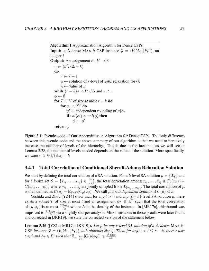
CHAPTER 3. A BIRTHDAY REPETITION THEOREM AND ITS APPLICATIONS 57
Algorithm 1 Approximation Algorithm for Dense CSPsInput: a ∆-dense MAX k-CSP instance G = (V,W , PS), aninteger iOutput: An assignment φ : V → Σr ← (k2i/∆ + k)do
r ← r + 1µ← solution of r-level of SAC relaxation for G.λ← value of µ
while (r − k)λ < k2i/∆ and r < nφ← ∅for T ⊆ V of size at most r − k do
for φT ∈ ΣT doφ′ ← independent rounding of µ|φTif val(φ′) > val(φ) then
φ← φ′.return φ
Figure 3.1: Pseudo-code of Our Approximation Algorithm for Dense CSPs. The only differencebetween this pseudo-code and the above summary of our algorithm is that we need to iterativelyincrease the number of levels of the hierarchy. This is due to the fact that, as we will see inLemma 3.28, the number of levels needed depends on the value of the solution. More specifically,we want r > k2i/(∆λ) + k
3.4.1 Total Correlation of Conditioned Sherali-Adams Relaxation SolutionWe start by defining the total correlation of a SA solution. For a k-level SA solution µ = XS andfor a k-size set S = xi1 , . . . , xik ∈
(Vk
), the total correlation among xi1 , . . . , xij is Cµ(xS) :=
C(σi1 ; . . . ;σik) where σi1 , . . . , σik are jointly sampled from Xxi1 ,...,xik. The total correlation of µis then defined as C(µ) = ES∼W [Cµ(xS)]. We call µ a κ-independent solution if C(µ) 6 κ.
Yoshida and Zhou [YZ14] show that, for any l > 0 and any (l + k)-level SA solution µ, thereexists a subset T of size at most l and an assignment φT ∈ ΣT such that the total correlationof (µ|φT ) is at most 3k log q
l∆ where ∆ is the density of the instance. In [MR17a], this bound wasimproved to k2 log q
l∆ via a slightly sharper analysis. Minor mistakes in those proofs were later foundand corrected in [JKR19]; we state the corrected version of the statement below.
Lemma 3.26 ([YZ14; MR17a; JKR19]). Let µ be any r-level SA solution of a ∆-dense MAX k-CSP instance G = (V,W , PS) with alphabet size q. Then, for any 0 < l 6 r − k, there existst 6 l and φT ∈ Σt such that ET∼(Vt )[C(µ|φT )] 6 k2 log q
l∆ .
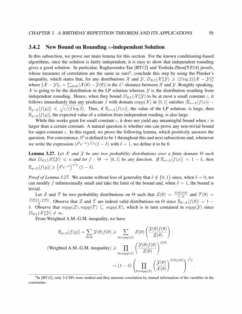
CHAPTER 3. A BIRTHDAY REPETITION THEOREM AND ITS APPLICATIONS 58
3.4.2 New Bound on Rounding κ-independent SolutionIn this subsection, we prove our main lemma for this section. For the known conditioning-basedalgorithms, once the solution is fairly independent, it is easy to show that independent roundinggives a good solution. In particular, Raghavendra-Tan [RT12] and Yoshida-Zhou[YZ14] proofs,whose measures of correlation are the same as ours6, conclude this step by using the Pinsker’sinequality, which states that, for any distributions X and Y , DKL(X‖Y) > (2 log 2)‖X − Y‖2
1where ‖X −Y‖1 = ∑
θ∈Θ |X (θ)−Y(θ)| is the L1-distance between X and Y . Roughly speaking,X is going to be the distribution in the LP solution whereas Y is the distribution resulting fromindependent rounding. Hence, when they bound DKL(X‖Y) to be at most a small constant ε, itfollows immediately that any predicate f with domain supp(X ) in [0, 1] satisfies |Ex∼X [f(x)] −Ey∼Y [f(y)]| 6
√ε/(2 log 2). Thus, if Ex∼X [f(x)], the value of the LP solution, is large, then
Ey∼Y [f(y)], the expected value of a solution from independent rouding, is also large.While this works great for small constant ε, it does not yield any meaningful bound when ε is
larger than a certain constant. A natural question is whether one can prove any non-trivial boundfor super-constant ε. In this regard, we prove the following lemma, which positively answers thequestion. For convenience, 00 is defined to be 1 throughout this and next subsections and, wheneverwe write the expression (δδe−κ)
11−δ (1− δ) with δ = 1, we define it to be 0.
Lemma 3.27. Let X and Y be any two probability distributions over a finite domain Θ suchthat DKL(X‖Y) 6 κ and let f : Θ → [0, 1] be any function. If Ex∼X [f(x)] = 1 − δ, then
Ey∼Y [f(y)] >(δδe−κ
) 11−δ (1− δ).
Proof of Lemma 3.27. We assume without loss of generality that δ /∈ 0, 1 since, when δ = 0, wecan modify f infinitesimally small and take the limit of the bound and, when δ = 1, the bound istrivial.
Let Z and T be two probability distributions on Θ such that Z(θ) = X (θ)f(θ)1−δ and T (θ) =
X (θ)(1−f(θ))δ
. Observe that Z and T are indeed valid distributions on Θ since Eθ∼X [f(θ)] = 1 −δ. Observe that supp(Z), supp(T ) ⊆ supp(X ), which is in turn contained in supp(Y) sinceDKL(X‖Y) 6=∞.
From Weighted A.M.-G.M. inequality, we have
Ey∼Y [f(y)] =∑θ∈ΘY(θ)f(θ) >
∑θ∈supp(Z)
Z(θ)(Y(θ)f(θ)Z(θ)
)
(Weighted A.M.-G.M. inequality) >∏
θ∈supp(Z)
(Y(θ)f(θ)Z(θ)
)Z(θ)
= (1− δ) ∏θ∈supp(Z)
(Y(θ)X (θ)
)X (θ)f(θ) 1
1−δ
.
6In [RT12], only 2-CSPs were studied and they measure correlation by mutual information of the variables in theconstraints.
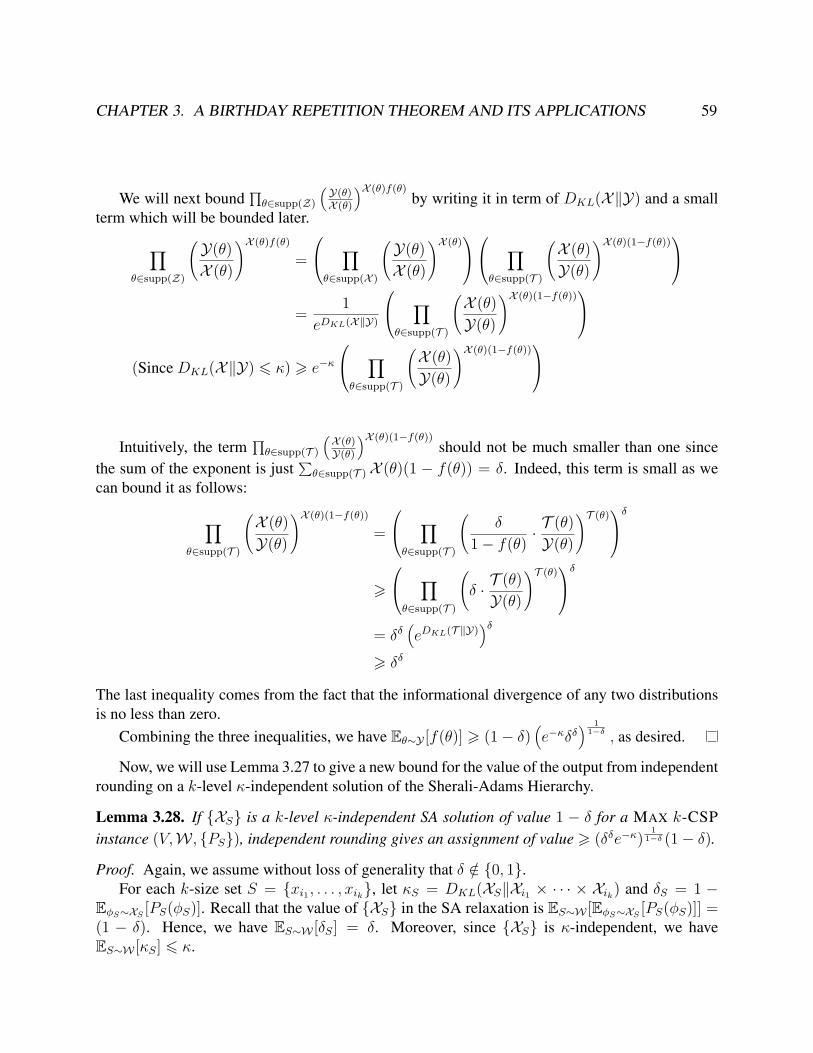
CHAPTER 3. A BIRTHDAY REPETITION THEOREM AND ITS APPLICATIONS 59
We will next bound∏θ∈supp(Z)
(Y(θ)X (θ)
)X (θ)f(θ)by writing it in term of DKL(X‖Y) and a small
term which will be bounded later.
∏θ∈supp(Z)
(Y(θ)X (θ)
)X (θ)f(θ)
= ∏θ∈supp(X )
(Y(θ)X (θ)
)X (θ) ∏
θ∈supp(T )
(X (θ)Y(θ)
)X (θ)(1−f(θ))
= 1eDKL(X‖Y)
∏θ∈supp(T )
(X (θ)Y(θ)
)X (θ)(1−f(θ))
(Since DKL(X‖Y) 6 κ) > e−κ
∏θ∈supp(T )
(X (θ)Y(θ)
)X (θ)(1−f(θ))
Intuitively, the term∏θ∈supp(T )
(X (θ)Y(θ)
)X (θ)(1−f(θ))should not be much smaller than one since
the sum of the exponent is just∑θ∈supp(T )X (θ)(1 − f(θ)) = δ. Indeed, this term is small as we
can bound it as follows:
∏θ∈supp(T )
(X (θ)Y(θ)
)X (θ)(1−f(θ))
= ∏θ∈supp(T )
(δ
1− f(θ) ·T (θ)Y(θ)
)T (θ)δ
>
∏θ∈supp(T )
(δ · T (θ)Y(θ)
)T (θ)δ
= δδ(eDKL(T ‖Y)
)δ> δδ
The last inequality comes from the fact that the informational divergence of any two distributionsis no less than zero.
Combining the three inequalities, we have Eθ∼Y [f(θ)] > (1− δ)(e−κδδ
) 11−δ , as desired.
Now, we will use Lemma 3.27 to give a new bound for the value of the output from independentrounding on a k-level κ-independent solution of the Sherali-Adams Hierarchy.
Lemma 3.28. If XS is a k-level κ-independent SA solution of value 1 − δ for a MAX k-CSPinstance (V,W , PS), independent rounding gives an assignment of value > (δδe−κ)
11−δ (1− δ).
Proof. Again, we assume without loss of generality that δ /∈ 0, 1.For each k-size set S = xi1 , . . . , xik, let κS = DKL(XS‖Xi1 × · · · × Xik) and δS = 1 −
EφS∼XS [PS(φS)]. Recall that the value of XS in the SA relaxation is ES∼W [EφS∼XS [PS(φS)]] =(1 − δ). Hence, we have ES∼W [δS] = δ. Moreover, since XS is κ-independent, we haveES∼W [κS] 6 κ.
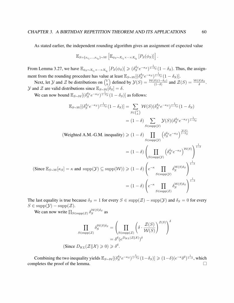
CHAPTER 3. A BIRTHDAY REPETITION THEOREM AND ITS APPLICATIONS 60
As stated earlier, the independent rounding algorithm gives an assignment of expected value
ES=xi1 ,...,xik∼W[EφS∼Xi1×···×Xik [PS(φS)]
].
From Lemma 3.27, we have EφS∼Xi1×···×Xik [PS(φS)] > (δδSS e−κS)1
1−δS (1− δS). Thus, the assign-
ment from the rounding procedure has value at least ES∼W [(δδSS e−κS)1
1−δS (1− δS)].Next, let Y and Z be distributions on
(Vk
)defined by Y(S) = W(S)(1−δS)
(1−δ) and Z(S) = W(S)δSδ
.Y and Z are valid distributions since ES∼W [δS] = δ.
We can now bound ES∼W [(δδSS e−κS)1
1−δS (1− δS)] as follows:
ES∼W [(δδSS e−κS)1
1−δS (1− δS)] =∑
S∈(Vk)W(S)(δδSS e−κS)
11−δS (1− δS)
= (1− δ)∑
S∈supp(Y)Y(S)(δδSS e−κS)
11−δS
(Weighted A.M.-G.M. inequality) > (1− δ)∏
S∈supp(Y)
(δδSS e
−κS) Y(S)
1−δS
= (1− δ) ∏S∈supp(Y)
(δδSS e
−κS)W(S)
11−δ
(Since ES∼W [κS] = κ and supp(Y) ⊆ supp(W)) > (1− δ)e−κ ∏
S∈supp(Y)δW(S)δSS
11−δ
= (1− δ)e−κ ∏
S∈supp(Z)δW(S)δSS
11−δ
The last equality is true because δS = 1 for every S ∈ supp(Z) − supp(Y) and δS = 0 for everyS ∈ supp(Y)− supp(Z).
We can now write∏S∈supp(Z) δ
W(S)δSS as
∏S∈supp(Z)
δW(S)δSS =
∏S∈supp(Z)
(δ · Z(S)W(S)
)Z(S)δ
= δδ(eDKL(Z‖X ))δ
(Since DKL(Z‖X ) > 0) > δδ.
Combining the two inequality yields ES∼W [(δδSS e−κS)1
1−δS (1−δS)] > (1−δ)(e−κδδ)1
1−δ , whichcompletes the proof of the lemma.
CHAPTER 3. A BIRTHDAY REPETITION THEOREM AND ITS APPLICATIONS 61
3.4.3 New Approximation Guarantee for the AlgorithmWith Lemma 3.26 and Lemma 3.28 set up, we now prove the algorithmic guarantee for Algo-rithm 1.
Theorem 3.29. For any MAX k-CSP instance G of value 1−δ > 0 and density ∆ > 0, Algorithm 1runs in time NO( ki
(1−δ)∆) and outputs an assignment of value at least (1− δ)δδ
1−δ /q1/i.
Proof. Observe that the running time is (nq)O(r) where r is the maximum level of the SAC relax-ation solved by the algorithm. Since the program is a relaxation of MAX k-CSP, λ is always atleast 1 − δ. By the condition of the loop, r is at most 1 + k + k2i
(1−δ)∆ . Hence, the running time of
the algorithm is NO( ki(1−δ)∆).
Next, we will argue about the value of the output assignment. From Lemma 3.26, there existsa set T ⊆ V of size at most k2i
λ∆ and an assignment φT ∈ ΣT such that µ|φT is an (λ log q/i)-independent solution. Moreover, from how SAC program is defined, we know that valSA(µ|φT ) >λ. As a result, from Lemma 3.28, independent rounding on µ|φT gives an assignment of value atleast
((1− λ)1−λe−λ log q/i) 1λλ = λ(1− λ)
1−λλ /q1/i.
Finally, since |T | 6 k2iλ∆ 6 r − k, it is considered in the conditioning step of the algorithm. Thus,
the output assignment is of value at least λ(1− λ) 1−λλ /q1/i > (1− δ)δ
δ1−δ /q1/i.
Observe that, when the instance is satisfiable, δ = 0 and the value of the output assignment is atleast 1/q1/i. By taking i to be large enough, one arrives at a quasi-polynomial time approximationscheme (QPTAS) for dense MAX k-CSP, as stated below. We note that our algorithm unfortu-nately does not give a QPTAS for the nonsatisfiable case since we also lose an additional factor ofδ
δ1−δ in the value of the output solution.
Corollary 3.30. There is an algorithm that, given a satisfiable ∆-dense MAX k-CSP instance Gand any 1/2 > ε > 0, runs inNO( k log q
ε∆ ) time and output an assignment to G of value at least 1−ε.
Proof. Run Algorithm 1 with i = log q/ log(1 + ε). From Theorem 3.29, the output assignmenthas value at least q1/i = 1/(1 + ε) > 1 − ε while the running time is NO( ki∆ ). Finally, weconclude by observing that i = log q/ log(1+ε) 6 O(log q/ε), which follows from the Bernoulli’sinequality.
3.5 Discussion and Open ProblemsWe prove that birthday repetition can amplify gap in hardness of approximation. This has severalinteresting consequences to the approximability of dense MAX k-CSP. First, we prove almost-polynomial ratio polynomial-time ETH-hardness for the problem. Second, we show, assuming thestronger Gap-ETH, that it is impossible to approximate dense MAX 2-CSP to within factor N1/i
CHAPTER 3. A BIRTHDAY REPETITION THEOREM AND ITS APPLICATIONS 62
in time N O(i). Third, we prove a similar integrality gap for Lasserre relaxation of the problem.Moreover, we provide an approximation algorithm that almost matches our lower bound based onGap-ETH and the Lasserre integrality gap.
While our results settle down the approximability of dense MAX k-CSP up to the dependencyon k and a factor of polylogi in the exponent, our work also raises many interesting questions,which we list below.
• What is the right dependency on ε in the birthday repetition theorem? It is unclear whetherthe dependency of 1/ log(1/ε) is needed in the exponent. We remark here that, in the casethatQ is uniform over a regular graph, Ko [Ko18] gives a lower bound that is tight up to thefactor of 1/ log(1/ε) in the exponent.
• Can our approximation algorithm for dense k-CSP be made to run in qOk(i)+NO(1) time? Asstated earlier, Yaroslavtev’s algorithm [Yar14] runs in qOk(log q/ε2) +NO(1) time and providesan ε additive approximation to the problem. As for our algorithm, we can, in fact, turnthe condioning step into a randomized algorithm where we just randomly pick a set andan assignment to condition7, which takes only linear time. The bottleneck, however, issolving the linear program (SAC relaxation), which takes NΩ(r) time where r is the numberof rounds. Related to this, Barak et al. [BRS11] showed that their Lasserre hierarchy-basedalgorithm runs in 2rNO(1) instead of NO(r) time8. It is an interesting question to ask whetherour algorithm can also be sped up using their technique.
• Can Lemma 3.27 be used to prove new approximation guarantees for other problems?Lemma 3.27 is a generic bound on the (multiplicative) difference of expectations of a func-tion on two distributions based on their informational divergence. Hence, it may yield newapproximation guarantees for other correlation-based algorithms as well.
• Is it possible to prove a result similar to Lemma 3.28 without losing a constant factor?Lemma 3.28 at the heart of our approximatin algorithm has one drawback: when δ is notzero, we always lose a factor of δ
δ1−δ . While the loss here is only constant (since it is min-
imized when δ → 1 which gives δδ
1−δ > 0.367), it prevents us from getting a QPTAS fornon-satisfiable dense MAX k-CSP. If this factor can be removed, we can establish the num-ber of levels needed for any approximation ratio from as large as polynomial in q to as smallas any constant.
7This is because the bound in Lemma 3.26 on total correlation of conditioned solution actually holds (in expecta-tion) for random T and φT sampled according to the marginal distribution XT .
8Note here that the number of rounds r used in Barak et al.’s algorithm is polynomial in the alphabet size q.
63
Chapter 4
Densest k-Subgraph with PerfectCompleteness
In the DENSEST k-SUBGRAPH (DkS) problem, we are given an undirected graph G on n verticesand a positive integer k 6 n. The goal is to find a set S of k vertices such that the induced subgraphon S has maximum number of edges. Since the size of S is fixed, the problem can be equivalentlystated as finding a k-subgraph (i.e. subgraph on k vertices) with maximum density.
DENSEST k-SUBGRAPH, a natural generalization of k-CLIQUE [Kar72], was first formulatedand studied by Kortsarz and Peleg [KP93] in the early 90s. Since then, it has been the subjectof intense study in the context of approximation algorithm and hardness of approximation [FS97;SW98; FL01; FKP01; AHI02; Fei02; Kho06; GL09; RS10; Bha+10; Alo+11; Bha+12; Bar15;Bra+17]. Despite this, its approximability still remains wide open and is considered by some to bean important open question in approximation algorithms [Bha+10; Bha+12; Bra+17].
On the algorithmic front, Kortsarz and Peleg [KP93], in the same work that introduced the prob-lem, gave a polynomial-time O(n0.3885)-approximation algorithm for DkS. Feige, Kortsarz andPeleg [FKP01] later provided an O(n1/3−δ)-approximation for the problem for some constant δ ≈1/60. This approximation ratio was the best known for almost a decade 1 until Bhaskara et al. [Bha+10]invented a log-density based approach which yielded anO(n1/4+ε)-approximation for any constantε > 0. This remains the state-of-the-art approximation algorithm for DkS.
While the above algorithms demonstrate the main progresses of approximations of DkS ingeneral case over the years, many special cases have also been studied. Most relevant to ourwork is the case where the optimal k-subgraph has high density (e.g. is a k-Clique), in whichbetter approximations are known [FS97; ST08; MM15; Bar15]. The first and most representativealgorithm of this kind is that of Feige and Seltser [FS97], which provides the following guarantee:when the input graph contains a k-clique, the algorithm can find an (1 − ε)-dense k-subgraph innO(logn/ε) time. We will refer to this problem of finding densest k-subgraph when the input graph ispromised to have a k-clique DENSEST k-SUBGRAPH with perfect completeness. DkS with perfect
1Around the same time as Bhaskara et al.’s work [Bha+10], Goldstein and Langberg [GL09] presented an algo-rithm with approximation ratio O(n0.3159), which is slightly better than [FKP01] but is worse than [Bha+10].
CHAPTER 4. DENSEST k-SUBGRAPH WITH PERFECT COMPLETENESS 64
completeness should of course reminds us of dense CSPs from the previous section, as both havequasi-polynomial time algorithm and hence are unlikely to be NP-hard to approximate. Moreover,Feige and Seltser’s algorithm [FS97] can2 achieve approximation ratio nε in time nO(1/ε), furthersuggesting the similarity between dense CSPs and DkS with perfect completeness.
Although many algorithms have been devised for DkS, relatively little is known regarding itshardness of approximation. While it is commonly believed that the problem is hard to approximateto within some polynomial ratio [Alo+11; Bha+12], not even a constant factor NP-hardness of ap-proximation is known. To circumvent this, Feige [Fei02] came up with a hypothesis that a random3SAT formula is hard to refute in polynomial time and proved that, assuming this hypothesis, DkSis hard to approximate to within some constant factor.
Alon et al. [Alo+11] later used a similar conjecture regarding random k-AND to rule outpolynomial-time algorithms for DkS with any constant approximation ratio. Moreover, theyproved hardnesses of approximation of DkS under the following Planted Clique Hypothesis [Jer92;Kuc95]: there is no polynomial-time algorithm that can distinguish between a typical Erdos-Rényirandom graph G(n, 1/2) and one in which a clique of size polynomial in n (e.g. n1/3) is planted.Assuming this hypothesis, Alon et al. proved that no polynomial-time algorithm approximatesDkS to within any constant factor. They also showed that, when the hypothesis is strengthenedto rule out not only polynomial-time but also super-polynomial time algorithms for the PlantedClique problem, their inapproximability guarantee for DkS can be improved. In particular, if nonO(
√logn)-time algorithm solves the Planted Clique problem, then 2O(log2/3 n)-approximation for
DkS cannot be achieved in polynomial time.There are also several inapproximability results of DkS based on worst-case assumptions.
Khot [Kho06] showed, assuming NP 6⊆BPTIME(2nε) for some constant ε > 0, that no polynomial-time algorithm can approximate DkS to within (1 + δ) factor where δ > 0 is a constant dependingonly on ε; the proof is based on a construction of a “quasi-random” PCP, which is then used inplace of a random 3SAT in a reduction similar to that from [Fei02].
While no inapproximability of DkS is known under the Unique Games Conjecture, Raghaven-dra and Steurer [RS10] showed that a strengthened version of it, in which the constraint graph isrequired to satisfy a “small-set expansion” property, implies that DkS is hard to approximate towithin any constant ratio.
Recently, Braverman et al. [Bra+17], showed, assuming ETH, that, for some constant ε > 0,no nO(logn)-time algorithm can approximate DENSEST k-SUBGRAPH with perfect completenessto within (1 + ε) factor. Their result matches almost exactly with the previously mentioned Feige-Seltser algorithm [FS97]. In fact, their construction uses the “label-extended graph” of the birthdayrepetition game described in the previous section.
Since none of these inapproximability results achieve a polynomial ratio, there have been ef-forts to prove better lower bounds for restricted classes of algorithms. For example, Bhaskaraet al. [Bha+12] provided polynomial ratio lower bounds against SDP relaxations of DkS. Specif-ically, for the Sum-of-Squares hierarchy, they showed integrality gaps of n2/53−ε and nε against
2This guarantee was not stated explicitly in [FS97] but it can be easily achieved by changing the degree thresholdin their algorithm DenseSubgraph from (1− ε)n to nε.
CHAPTER 4. DENSEST k-SUBGRAPH WITH PERFECT COMPLETENESS 65
nΩ(ε) and n1−O(ε) levels of the hierarchy respectively. (See also [Man15; Chl+17b] in which 2/53in the exponent was improved to 1/14.) Unfortunately, it is unlikely that these lower bounds can betranslated to inapproximability results and the question of whether any polynomial-time algorithmcan achieve subpolynomial approximation ratio for DkS remains an intriguing open question.
Our ResultsWe rule out, under the exponential time hypothesis (Hypothesis 1), polynomial-time approximationalgorithms for DkS (even with perfect completeness) with slightly subpolynomial ratio:
Theorem 4.1. There exists c > 0 such that, assuming ETH, no polynomial-time algorithm can,given a graph G on n vertices and a positive integer k 6 n, distinguish between the following twocases:
• There exist k vertices of G that induce a k-clique.
• Every k-subgraph of G has density at most n−1/(log logn)c .
If we assume the stronger gap exponential time hypothesis (Hypothesis 3), the ratio can beimproved to ng(n) for any 3 g ∈ o(1). In fact, we can get an even finer-grained trade-off: to achievenε-approximation, the running time of the algorithm has to be nΩ(1/ε1/3), as formalized below.
Theorem 4.2. For any ν > 0, assuming Gap-ETH, there is no algorithm that, given any graph
G and any ε > 0, runs in nO
(1
ε1/3·log4/3+ν (1/ε)
)time and can distinguish between the following two
cases:
• There exist k vertices of G that induce a k-clique.
• Every k-subgraph of G has density at most n−ε.
Recall that, for DkS with perfect completeness, the aforementioned Feige-Seltser algorithmachieves an nε-approximation in time nO(1/ε) for every ε > 0 [FS97]. Our above lower boundindeed confirms that, to get better approximation ratio, more running time is needed. Nonetheless,it does not yet resolve the correct trade-off between these parameters, and it remains an interestingopen question to bridge the gap of the running time between nO(1/ε) in the upper bound of [FS97]and nΩ(1/ε1/3) in our above lower bound.
Comparison to Previous Results. In terms of inapproximability ratios, the ratios ruled outin this work are almost polynomial and provides a vast improvement over previous results. Priorto our result, the best known ratio ruled out under any worst case assumption is only any con-stant [RS10] and the best ratio ruled out under any average case assumption is only 2O(log2/3 n) [Alo+11].In addition, our results also have perfect completeness, which was only achieved in [Bra+17] underETH and in [Alo+11] under the Planted Clique Hypothesis but not in [Kho06; Fei02; RS10].
3Recall that g ∈ o(1) if and only if limn→∞ g(n) = 0.

CHAPTER 4. DENSEST k-SUBGRAPH WITH PERFECT COMPLETENESS 66
Regarding the assumptions our results are based upon, the average case assumptions usedin [Fei02; Alo+11] are incomparable to ours. The assumption NP 6⊆BPTIME(2nε) used in [Kho06]is also incomparable to ours since, while not stated explicitly, ETH and Gap-ETH by defaultfocus only on deterministic algorithms and our reductions are also deterministic. The strength-ened Unique Games Conjecture used in [RS10] is again incomparable to ours as it is a statementthat a specific problem is NP-hard. Finally, although Braverman et al.’s result [Bra+17] also re-lies on ETH, its relation to our results is more subtle. Specifically, their reduction time is only2Θ(√m) where m is the number of clauses, meaning that they only need to assume that 3SAT /∈
DTIME(2Θ(√m)) to rule out a constant ratio polynomial-time approximation for DkS. However, as
we will see in Theorem 4.4, even to achieve a constant gap, our reduction time is 2Ω(m3/4). Hence,if 3SAT somehow ends up in DTIME(2Θ(m3/4)) but outside of DTIME(2Θ(
√m)), their result will
still hold whereas ours will not even imply constant ratio inapproximability for DkS.Implications of Our Results. One of the reasons that DkS has received significant atten-
tion in the approximation algorithm community is due to its connections to many other problems.Most relevant to our work are the problems to which there are reductions from DkS that preserveapproximation ratios to within some polynomial4. These problems include DENSEST AT-MOST-k-SUBGRAPH [AC09], SMALLEST m-EDGE SUBGRAPH [CDK12], STEINER k-FOREST [HJ06]and QUADRATIC KNAPSACK [Pis07]. For brevity, we do not define these problems here. We referinterested readers to cited sources for their definitions and reductions from DkS to respective prob-lems. We also note that this list is by no means exhaustive and there are indeed numerous otherproblems with similar known connections to DkS (see e.g. [Haj+06; KS07; Kor+11; CHK11;HIM11; LNV14; Che+15a; CL15; CZ15; SFL15; TV15; Chl+16; Chu+15; Lee16]). Our resultsalso imply hardness of approximation results with similar ratios to DkS for such problems:
Corollary 4.3. For some c > 0, assuming ETH, there is no polynomial-time n1/(log logn)c-approximationalgorithm for DENSEST AT-MOST-k-SUBGRAPH, SMALLEST m-EDGE SUBGRAPH, STEINER k-FOREST, QUADRATIC KNAPSACK. Moreover, for any function f ∈ o(1), there is no polynomial-time nf(n)-approximation algorithm for any of these problems, unless Gap-ETH is false.
4.1 The Reduction and Proofs of The Main TheoremsThe reduction from Gap-3SAT to DkS is simple. Given a 3SAT formula φ on n variables x1, . . . , xnand an integer 1 6 ` 6 n, we construct a graph5 Gφ,` = (Vφ,`, Eφ,`) as follows:
4These are problems whose O(ρ)-approximation gives an O(ρc)-approximation for DkS for some constant c.5For interested readers, we note that our graph is not the same as the FGLSS graph [Fei+91] of the PCP in which
the verifier reads ` random variables and accepts if no clause is violated; while this graph has the same vertex set asours, the edges are different since we check that no clause between the two vertices is violated, which is not checkedin the FGLSS graph. It is possible to modify our proof to make it work for this FGLSS graph. However, the soundnessguarantee for the FGLSS graph is worse.
CHAPTER 4. DENSEST k-SUBGRAPH WITH PERFECT COMPLETENESS 67
• Its vertex set Vφ,` contains all partial assignments to ` variables. That is, each vertex is(xi1 , bi1), . . . , (xi` , bi`) where xi1 , . . . , xi` are ` distinct variables and bi1 , . . . , bi` ∈ 0, 1are the bits assigned to them.
• We connect two vertices (xi1 , bi1), . . . , (xi` , bi`) and (xi′1 , bi′1), . . . , (xi′`, bi′
`) by an edge
iff the two partial assignments are consistent (i.e. no variable is assigned 0 in one vertex and1 in another), and, every clause in φ all of whose variables are from xi1 , . . . , xi` , xi′1 , . . . , xi′`is satisfied by the partial assignment induced by the two vertices.
Clearly, if val(φ) = 1, the(n`
)vertices corresponding to a satisfying assignment induce a
clique. Our main technical contribution is proving that, when val(φ) 6 1− ε, every(n`
)-subgraph
is sparse:
Theorem 4.4. For any d, ε > 0, there exists τ > 0 such that, for any 3SAT formula φ on nvariables such that val(φ) 6 1 − ε and each variable appears in at most d clauses and for anyinteger ` ∈ [n3/4/τ, n/2], any
(n`
)-subgraph of Gφ,` has density 6 2−τ`4/n3
.
We remark that there is nothing special about 3SAT; we can start with any boolean CSP and endup with a similar result, albeit the soundness deteriorates as the arity of the CSP grows. However,it is crucial that the variables are boolean; in fact, Braverman et al. [Bra+17] considered a graphsimilar to ours for 2CSPs but they were unable to achieve subconstant soundness since their vari-ables were not boolean6. Specifically, there is a non-boolean 2CSP with low value which resultsin the graph having a biclique of size >
(n`
)(see Appendix A of [Man17a]), i.e., one cannot get an
inapproximability ratio more than two starting from a non-boolean CSP.Once we have Theorem 4.4, the inapproximability results of DkS (Theorem 4.1 and 4.2) can
be easily proved by applying the theorem with appropriate choices of `. We defer these proofsto Subsection 4.1.2. For now, let us turn our attention to the proof of Theorem 4.4. Recall thatAlon’s lemma [Alo02] (Lemma 2.14) states that every dense graph contains many labelled copiesof bicliques. Equipped with this lemma, our proof strategy is to bound the number of labelledcopies of Kt,t in Gφ,` where t is to be chosen later.
Before we proceed with the proof, we note here that, while the overall proof strategy is similarto that of the previous chapter, here we have to bound the number of copies of bicliques in theconstructed graph whereas we previously only had to bound the number of copies of bicliques inthe constraint graph.
To bound the number of labelled copies ofKt,t inGφ,`, we will need some additional notations:
• First, let Aφ := (x1, 0), (x1, 1), . . . , (xn, 0), (xn, 1) be the set of all single-variable partialassignments. Observe that Vφ,` ⊆
(Aφ`
), i.e., each u ∈ Vφ,` is a subset of Aφ of size `.
• Let A : (Vφ,`)t → P(Aφ) be a “flattening” function that, on input T ∈ (Vφ,`)t, outputs theset of all single-variable partial assignments that appear in at least one vertex in T . In otherwords, when each vertex u is viewed as a subset ofAφ, we can writeA(T ) simply as
⋃u∈T u.
6Any satisfiable boolean 2CSP is solvable in polynomial time so one cannot start with a boolean 2CSP either.
CHAPTER 4. DENSEST k-SUBGRAPH WITH PERFECT COMPLETENESS 68
• Let Kt,t := (L,R) ∈ (Vφ,`)t × (Vφ,`)t | ∀u ∈ L, ∀v ∈ R, u 6= v ∧ (u, v) ∈ Eφ,` denotethe set of all labelled copies of Kt,t in Gφ,` and, for each A,B ⊆ Aφ, let Kt,t(A,B) :=(L,R) ∈ Kt,t | A(L) = A,A(R) = B denote the set of all (L,R) ∈ Kt,t with A(L) = Aand A(R) = B.
The number of labelled copies of Kt,t in Gφ,` can be written as
|Kt,t| =∑
A,B⊆Aφ|Kt,t(A,B)|. (4.1)
To bound |Kt,t|, we will prove the following bound on |Kt,t(A,B)|.
Lemma 4.5. Let φ, n, `, d and ε be as in Theorem 4.4. There exists λ > 0 depending only on d andε such that, for any t ∈ N and any A,B ⊆ Aφ, |Kt,t(A,B)| 6
(2−λ`2/n
(n`
))2t.
Before we prove the above lemma, let us see how Lemma 2.14 and Lemma 4.5 imply Theo-rem 4.4.
Proof of Theorem 4.4. Assume w.l.o.g. that λ 6 1. Pick τ = λ2/8 and t = (4/λ)(n2/`2). FromLemma 4.5 and (4.1), we have
|Kt,t| 6 24n ·(
2−λ`2/n(n
`
))2t
6 (2−λ`2/n)t ·(n
`
)2t
where the second inequality comes from our choice of t; note that t is chosen so that the 24n factoris consumed by 2−λ`2/n from Lemma 4.5. Finally, consider any
(n`
)-subgraph of Gφ,`. By the
above bound, it contains at most (2−λ`2/n)t ·(n`
)2tlabelled copies of Kt,t. Thus, from Lemma 2.14
and from ` > n3/4/δ, its density is at most 2 · 2−λ`2/(nt) = 2 · 2−2τ`4/n36 2−τ`4/n3 as desired.
We now move on to the proof of Lemma 4.5.
Proof of Lemma 4.5. First, notice that if (x, b) appears in A and (x,¬b) appears in B for somevariable x and bit b, then Kt,t(A,B) = ∅; this is because, for any L with A(L) = A and R withA(R) = B, there exist u ∈ L and v ∈ R that contain (x, b) and (x,¬b) respectively, meaning thatthere is no edge between u and v and, thus, (L,R) /∈ Kt,t(A,B). Hence, from now on, we canassume that, if (x, b) appears in one of A,B, then the other does not contain (x,¬b). Observe thatthis implies that, for each variable x, its assignments can appear in A and B at most two times7 intotal. This in turn implies that |A|+ |B| 6 2n.
Let us now argue that |Kt,t(A,B)| 6(n`
)2t; while this is not the bound we are looking for yet,
it will serve as a basis for our argument later. For every (L,R) ∈ Kt,t(A,B), observe that, since7This is where we use the fact that the variables are boolean. For non-boolean CSPs, each variable x can appear
more than two times in one of A or B alone, which can indeed be problematic (see Appendix A of [Man17a]).
CHAPTER 4. DENSEST k-SUBGRAPH WITH PERFECT COMPLETENESS 69
A(L) = A and A(R) = B, we have L ∈(A`
)tand R ∈
(B`
)t. This implies that Kt,t(A,B) ⊆(
A`
)t×(B`
)t. Hence,
|Kt,t(A,B)| 6(|A|`
)t(|B|`
)t. (4.2)
Moreover,(|A|`
)(|B|`
)can be further bounded as
(|A|`
)(|B|`
)= 1
(`!)2
`−1∏i=0
(|A| − i)(|B| − i) 6 1(`!)2
`−1∏i=0
(|A|+ |B|
2 − i)2
6
(n
`
)2
(4.3)
where the inequalities come from the AM-GM Inequality and from |A| + |B| 6 2n respectively.Combining (4.2) and (4.3) indeed yields |Kt,t(A,B)| 6
(n`
)2t.
Inequality (4.2) is very crude; we include all elements of(A`
)and
(B`
)as candidates for vertices
in L and R respectively. However, as we will see soon, only tiny fraction of elements of(A`
),(B`
)can actually appear in L,R when (L,R) ∈ Kt,t(A,B). To argue this, let us categorize the variablesinto three groups:
• x is terrible iff its assignments appear at most once in total inA andB (i.e. |(x, 0), (x, 1)∩A|+ |(x, 0), (x, 1) ∩B| 6 1).
• x is good iff, for some b ∈ 0, 1, (x, b) ∈ A∩B. Note that this implies that (x,¬b) /∈ A∪B.
• x is bad iff either (x, 0), (x, 1) ⊆ A or (x, 0), (x, 1) ⊆ B.
The next and last step of the proof is where birthday-type paradoxes come in. Before wecontinue, let us briefly demonstrate the ideas behind this step by considering the following extremecases:
• If all variables are terrible, then |A|+ |B| 6 n and (4.3) can be immediately tightened.
• If all variables are bad, assume w.l.o.g. that, for at least half of variables x’s, (x, 0), (x, 1) ⊆A. Consider a random element u of
(A`
). Since u is a set of random ` distinct elements of
A, there will, in expectation, be Ω(`2/n) variables x’s with (x, 0), (x, 1) ∈ u. However,the presence of such x’s means that u is not a valid vertex. Moreover, it is not hard to turnthis into the following probabilistic statement: with probability at most 2−Ω(`2/n), u containsat most one of (x, 0), (x, 1) for every variable x. In other words, only 2−Ω(`2/n) fraction ofelements of
(A`
)are valid vertices, which yields the desired bound on |Kt,t(A,B)|.
• If all variables are good, then A = B is simply an assignment to all the variables. Sinceval(φ) 6 1 − ε, at least εm clauses are unsatisfied by this assignment. As we will arguebelow, every element of
(A`
)that contains two variables from some unsatisfied clause cannot
CHAPTER 4. DENSEST k-SUBGRAPH WITH PERFECT COMPLETENESS 70
be in L for any (L,R) ∈ Kt,t(A,B). This means that there are Θε(m) > Ωε(n) prohibitedpairs of variables that cannot appear together. Again, similar to the previous case, it is nothard to argue that only 2−Ωε,d(`2/n) fraction of elements of
(A`
)can be candidates for vertices
of L.
To turn this intuition into a bound on |Kt,t(A,B)|, we need the following inequality. Its proofis straightforward and is deferred to Subsection 4.1.1.
Proposition 4.6. Let U be any set and P ⊆(U2
)be any set of pairs of elements of U such that each
element of U appears in at most q pairs. For any positive integer 2 6 r 6 |U |, the probability thata random element of
(Ur
)does not contain both elements of any pair in P is at most exp
(− |P |r
2
4q|U |2).
We are now ready to formalize the above intuition and finish the proof of Lemma 4.5. Forthe sake of convenience, denote the sets of good, bad and terrible variables by Xg, Xb and Xt
respectively. Moreover, let β := ε/(100d) and pick λ = min− log(1 − β/2), β/64, ε/(384d).To refine the bound on the size of Kt,t(A,B), consider the following three cases:
1. |Xt| > βn. Since each x ∈ Xt contributes at most one to |A| + |B|, |A| + |B| 6 (1 −β/2)(2n). Hence, we can improve (4.3) to
(|A|`
)(|B|`
)6(
(1−β/2)n`
)2. Thus, we have
|Kt,t(A,B)|(4.2)6
(|A|`
)t(|B|`
)t6
((1− β/2)n
`
)2t
6
((1− β/2)`
(n
`
))2t
6
(2−λ`2/n
(n
`
))2t
where the last inequality comes from λ 6 − log(1− β/2) and ` > `2/n.
2. |Xb| > βn. Since each x ∈ Xb appears either in A or B, one of A and B must containassignments to at least (β/2)n variables inXb. Assume w.l.o.g. thatA satisfies this property.Let XL
b be the set of all x ∈ Xb whose assignments appear in A. Note that |XLb | > (β/2)n.
Observe that an element u ∈(A`
)is not a valid vertex if it contains both (x, 0) and (x, 1)
for some x ∈ XLb . We invoke Proposition 4.6 with U = A, P = (x, 0), (x, 1) | x ∈
XLb , q = 1 and r = `, which implies that a random element of
(A`
)does not contain any
prohibited pairs in P with probability at most exp(− |X
Lb |`
2
4|A|2
)6 exp
(− (β/2)n`2
4(2n)2
), which is
at most 2−2λ`2/n because λ 6 β/64. In other words, at most 2−2λ`2/n fraction of elements of(A`
)are valid vertices. This gives us the following bound:
|Kt,t(A,B)| 6(
2−2λ`2/n ·(|A|`
))t·(|B|`
)t (4.3)6
(2−λ`2/n
(n
`
))2t
.
3. |Xt| < βn and |Xb| < βn. In this case, |Xg| > (1 − 2β)n. Let S denote the set ofclauses whose variables all lie in Xg. Since each variable appears in at most d clauses,|S| > m− (2βn)d > (1− ε/2)m where the second inequality comes from our choice of βand from m > n/3.
CHAPTER 4. DENSEST k-SUBGRAPH WITH PERFECT COMPLETENESS 71
Consider the partial assignment f : Xg → 0, 1 induced by A and B, i.e., f(x) = b iff(x, b) ∈ A,B. Since val(φ) 6 1 − ε, the number of clauses in S satisfied by f is at most(1 − ε)m. Hence, at least εm/2 clauses in S are unsatisfied by f . Denote the set of suchclauses by SUNSAT.
Fix a clause C ∈ SUNSAT and let x, y be two different variables in C. We claim that x, ycannot appear together in any vertex of L for any (L,R) ∈ Kt,t(A,B). Suppose for thesake of contradiction that (x, f(x)) and (y, f(y)) both appear in u ∈ L for some (L,R) ∈Kt,t(A,B). Let z ∈ Xg be another variable8 in C. Since (z, f(z)) ∈ B, some vertex v ∈ Rcontains (z, f(z)). Thus, there is no edge between u and v in Gφ,`, which contradicts with(L,R) ∈ Kt,t.We can now appeal to Proposition 4.6 with U = A, q = 2d, r = ` and P be the pro-hibited pairs described above. This implies that with probability at most exp
(− |P |`
2
8d|A|2)6
exp(− ε`2
192dn
), a random element of
(A`
)contains no prohibited pair from P . In other words,
at most exp(− ε`2
192dn
)fraction of elements of
(A`
)can be candidates for each element of L
for (L,R) ∈ Kt,t(A,B). This gives the following bound:
|Kt,t(A,B)| 6(
exp(− ε`2
192dn
)·(|A|`
))t·(|B|`
)t (4.3)6
(2−ε`2/(384dn) ·
(n
`
))2t
.
Since we picked λ 6 ε/(384d), |Kt,t(A,B)| is once again bounded above by(2−λ`2/n
(n`
))2t.
In all three cases, we have |Kt,t(A,B)| 6(2−λ`2/n
(n`
))2t, completing the proof of Lemma 4.5.
4.1.1 Proof of Proposition 4.6Proof of Proposition 4.6. We first construct P ′ ⊆ P such that each element of U appears in atmost one pair in P ′ as follows. Start out by marking every pair in P as active and, as long as thereare active pairs left, include one in P ′ and mark every pair that shares an element of U with thispair as inactive. Since each element of U appears in at most q pairs in P , we mark at most 2q pairsas inactive per each inclusion. This implies that |P ′| > |P |/(2q).
Suppose that P ′ = a1, b1, . . . , a|P ′|, b|P ′| where a1, b1, . . . , a|P ′|, b|P ′| are distinct ele-ments of U . Let u be a random element of
(Ur
). For each i = 1, . . . , |P ′|, we have
Pr[ai, bi 6⊆ u] = 1−
(|U |−2r−2
)(|U |r
)= 1− r(r − 1)
|U |(|U | − 1)8If C contains two variables, let z = x. Note that we can assume w.l.o.g. that C contains at least two variables.
CHAPTER 4. DENSEST k-SUBGRAPH WITH PERFECT COMPLETENESS 72
(Since r − 1 > r/2 for all r > 2) 6 1− r2
2|U |2
(Since 1− z 6 exp(−z) for all z ∈ R) 6 exp(− r2
2|U |2
).
If u does not contain both elements of any pairs in P , it does not contain both elements of anypairs in P ′. The probability of the latter can be written as
Pr|P ′|∧i=1ai, bi 6⊆ u
=|P ′|∏i=1
Prai, bi 6⊆ u
∣∣∣∣∣∣i−1∧j=1aj, bj 6⊆ u
.In addition, since a1, b1, . . . , a|P ′|, b|P ′| are distinct, it is not hard to see that Pr[ai, bi 6⊆ u] >
Pr[ai, bi 6⊆ u
∣∣∣ ∧i−1j=1aj, bj 6⊆ u
]. Hence, we have
Pr|P ′|∧i=1ai, bi 6⊆ u
=|P ′|∏i=1
Pr[ai, bi 6⊆ u] 6(
exp(− r2
2|U |2
))|P ′|= exp
(−|P
′|r2
2|U |2
)
6 exp(− |P |r
2
4q|U |2
),
completing the proof of Proposition 4.6.
4.1.2 Proofs of Inapproximability Results of DkSIn this subsection, we prove Theorem 4.1 and 4.2. The proof of Theorem 4.1 is simply by combin-ing Dinur’s PCP Theorem and Theorem 4.4 with ` = m/polylogm, as stated below.
Proof of Theorem 4.1. For any 3SAT formula ϕ with m clauses, use Theorem 2.2 to produce φwith m′ = O(mpolylogm) clauses such that each variable appears in at most d clauses. Let ζ bea constant such that m′ = O(m logζm) and let ` = m/ log2m. Let us consider the graph Gφ,`
with k =(n`
)where n is the number of variables of φ. Let N be the number of vertices of Gφ,`.
Observe that N = 2`(n`
)6 n2` 6 (m′)O(`) = 2O(` logm′) = 2o(m).
If ϕ is satisfiable, φ is also satisfiable and it is obvious that Gφ,` contains an induced k-clique. Otherwise, If ϕ is unsatisfiable, val(φ) 6 1 − ε. From Theorem 4.4, any k-subgraphof Gφ,` has density at most 2−Ω(`4/n3) 6 2−Ω(m/ log3ζ+8 m) = N−Ω(1/(log logN)3ζ+8), which is at mostN−1/(log logN)3ζ+9 when m is sufficiently large. Hence, if there is a polynomial-time algorithm thatcan distinguish between the two cases in Theorem 4.1 when c = 3ζ + 9, then there also exists analgorithm that solves 3SAT in time 2o(m), contradicting with ETH.
The proof of Theorem 4.2 is even simpler since, under Gap-ETH, we have the gap version of3SAT to begin with. Hence, we can directly apply Theorem 4.4 without going through Dinur’sPCP:
CHAPTER 4. DENSEST k-SUBGRAPH WITH PERFECT COMPLETENESS 73
Proof of Theorem 4.2. Let φ be any 3SAT formula with m clauses such that each variable appearsin O(1) clauses. For any constant 1 > γ, ν > 0, let ` = m
(γ1/3 · log1/3+ν/2(1/γ)
)and consider
the graph Gφ,` with k =(n`
)where n is the number of variables of φ. The number of vertices N of
Gφ,` is 2`(n`
)6 2`
(en`
)`6 2O(` log(m/`)) = 2O(m(γ1/3·log4/3+ν/2(1/γ))).
The completeness is again obvious. For the soundness, if val(φ) 6 1 − ε, from Theo-rem 4.4, any k-subgraph of Gφ,` has density at most 2−Ω(`4/n3) 6 2−Ω(mγ4/3 log4/3+2ν(1/γ)) 6N−Ω(γ·log3ν/2(1/γ)), which is at most N−γ when γ is sufficiently small. Now suppose contrapos-itively that, for some ν > 0, there is an algorithm that, given a graph G and γ, runs in time
NO
(1
γ1/3 log4/3+ν (γ)
)and can distinguish between the two cases in Theorem 4.2. By running this
algorithm on Gφ,`, we can solve Gap-3SAT in time 2O(
m
logν/2(1/γ)
); by picking a sufficiently small
γ, this contradicts with Gap-ETH.
4.2 Discussion and Open QuestionsIn this chapter, we provide a subexponential time reduction from the gap version of 3SAT to DkSand prove that it establishes an almost-polynomial ratio hardness of approximation of the latterunder ETH and Gap-ETH. Even with our results, however, approximability of DkS still remainswide open. Namely, it is still not known whether it is NP-hard to approximate DkS to within someconstant factor, and, no polynomial ratio hardness of approximation is yet known.
Although our results appear to almost resolve the second question, it still seems out of reachwith our current knowledge of hardness of approximation. In particular, to achieve a polynomialratio hardness for DkS, it is plausible that one has to prove a long-standing conjecture called thesliding scale conjecture (SSC) [Bel+93]. In short, SSC essentially states that LABEL COVER is NP-hard to approximate to within some polynomial ratio. Note here that polynomial ratio hardness forLABEL COVER is not even known under stronger assumptions such as ETH or Gap-ETH; we referthe readers to [Din16] and Chapter 9 for more detailed discussions on the topic.
There is in fact an approximation preserving reduction from DkS to LABEL COVER [CHK11]but it does not provide perfect completeness, which is required in SSC; this leaves a possibilitythat a polynomial ratio hardness of approximation of DkS can be achieved without resolving SSC.
Apart from the approximability of DkS, our results also prompt the following natural ques-tion: since previous techniques, such as Feige’s Random 3SAT Hypothesis [Fei02], Khot’s Quasi-Random PCP [Kho06], Unique Games with Small Set Expansion Conjecture [RS10] and thePlanted Clique Hypothesis [Jer92; Kuc95], that were successful in showing inapproximabilityof DkS also gave rise to hardnesses of approximation of many problems that are not known tobe APX-hard including SPARSEST CUT, MIN BISECTION, BALANCED SEPARATOR, MINIMUM
LINEAR ARRANGEMENT and 2-CATALOG SEGMENTATION [AMS07; Sak10; RST12], is it possi-ble to modify our construction to prove inapproximability for these problems as well? An evidencesuggesting that this may be possible is the case of ε-approximate Nash Equilibrium with ε-optimalwelfare, which was first proved to be hard under the Planted Clique Hypothesis by Hazan and

CHAPTER 4. DENSEST k-SUBGRAPH WITH PERFECT COMPLETENESS 74
Krauthgamer [HK11] before Braverman, Ko and Weinstein proved that the problem was also hardunder ETH using the birthday repetition framework [BKW15].
75
Chapter 5
VC Dimension and Littlestone’s Dimension
A common and essential assumption in learning theory is that the concepts we want to learn comefrom a nice, simple concept class, or (in the agnostic case) they can at least be approximated by aconcept from a simple class. When the concept class is sufficiently simple, there is hope for good(i.e. sample-efficient and low-error) learning algorithms.
There are many different ways to measure the simplicity of a concept class. The most influentialmeasure of simplicity is the VC Dimension, which captures learning in the PAC model. We alsoconsider Littlestone’s Dimension [Lit88], which corresponds to minimizing mistakes in onlinelearning (see Section 5.2 for definitions). When either dimension is small, there are algorithmsthat exploit the simplicity of the class, to obtain good learning guarantees.
We consider the most optimistic setting where the entire universe and concept class are givenas explicit input (a binary matrix whose (x,C)-th entry is 1 iff element x belongs to conceptC). In this setting, both VC Dimension and Littlestone’s Dimension can be computed (exactly1)in nO(logn) time2. Hence, similar to problems considered earlier in this thesis, the problem ofcomputing these dimensions are unlikely to be NP-hard.
Nonetheless, two decades ago, it was shown (under appropriate computational complexity as-sumptions) that neither dimension can be computed in polynomial time [PY96; FL98]. UnderETH, their reduction also yields a tight running time lower bound of nΩ(logn) to compute the twodimensions. Such computational intractability of computing the (VC, Littlestone’s) dimension ofa concept class suggests that even in cases where a simple structure exists, it may be inaccessibleto computationally bounded algorithms (see Discussion below).
We prove a (almost) tight running time lower bound, similar to those implied by [PY96; FL98],that hold even against approximation algorithms, as stated below.
Theorem 5.1 (Hardness of Approximating VC Dimension). Assuming Randomized ETH, approx-imating VC Dimension to within a (1/2 + o(1))-factor requires nlog1−o(1) n time.
1As discussed in Section 1.1.3, this is unlike dense CSPs and DkS with perfect completeness, for which the exactversions are NP-hard but QPTASs exist.
2For VC Dimension, this is because the dimension itself is at most logn and hence we can simply enumerate allsets S ⊆ U or size at most logn and check whether it is shattered. For Littlestone’s Dimension, there is a simpledivide-and-conquer algorithm for it (see Section 5.4.4).
CHAPTER 5. VC DIMENSION AND LITTLESTONE’S DIMENSION 76
Theorem 5.2 (Hardness of Approximating Littlestone’s Dimension). There exists an absolute con-stant ε > 0 such that, assuming Randomized ETH, approximating Littlestone’s Dimension towithin a (1− ε)-factor requires nlog1−o(1) n time.
5.1 Interpretation of the ResultsAs we mentioned before, the computational intractability of computing the (VC, Littlestone’s)dimension of a concept class suggests that even in cases where a simple structure exists, it may beinaccessible to computationally bounded algorithms. We note however that it is not at all clear thatany particular algorithmic applications are immediately intractable as a consequence of our results.
Consider for example the adversarial online learning zero-sum game corresponding to Lit-tlestone’s Dimension: At each iteration, Nature presents the learner with an element from theuniverse; the learner attempts to classify the element, and loses a point for every wrong classifi-cation; at the end of the iteration, the correct (binary) classification is revealed. The Littlestone’sDimension is equal to the worst case loss of the Learner before learning the exact concept. (seeSection 5.2 for a more detailed definition.)
What can we learn from the fact that the Littlestone’s Dimension is hard to compute? Thefirst observation is that there is no efficient learner that can commit to a concrete mistake bound.But this does not rule out a computationally-efficient learner that plays optimal strategy and makesat most as many mistakes as the unbounded learner. We can, however, conclude that Nature’stask is computationally intractable! Otherwise, we could efficiently construct an entire worst-casemistake tree (for a concept class C, any mistake tree has at most |C| leaves, requiring |C|− 1 oraclecalls to Nature).
On a philosophical level, we think it is interesting to understand the implications of an in-tractable, adversarial Nature. Perhaps this is another evidence that the mistake bound model is toopessimistic?
Also, the only algorithm we know for computing the optimal learner’s decision requires com-puting the Littlestone’s Dimension. We think that it is an interesting open question whether anapproximately optimal computationally-efficient learner exists.
In addition, let us note that in the other direction, computing Littlestone’s Dimension exactlyimplies an exactly optimal learner. However, since the learner has to compute Littlestone’s Dimen-sion many times, we have no evidence that an approximation algorithm for Littlestone’s Dimensionwould imply any guarantee for the learner.
Finally, we remark that for either problem (VC or Littlestone’s Dimension), we are not awareof any non-trivial approximation algorithms.
5.1.1 TechniquesAs with our previous two chapters, we once again follow the “birthday repetition” framework.However, there are multiple unique challenges we have to overcome for both VC Dimension andLittlestone’s Dimension, as described below.
CHAPTER 5. VC DIMENSION AND LITTLESTONE’S DIMENSION 77
VC Dimension The first challenge we have to overcome in order to adapt this framework tohardness of approximation of VC Dimension is that the number of concepts involved in shatteringa subset S is 2|S|. Therefore any inapproximability factor we prove on the size of the shatteredset of elements, “goes in the exponent” of the size of the shattering set of concepts. Even a smallconstant factor gap in the VC Dimension requires proving a polynomial factor gap in the numberof shattering concepts (obtaining polynomial gaps via “birthday repetition” for simpler problemsis an interesting open problem [MR17a; Man17a]). Fortunately, having a large number of conceptsis also an advantage: we use each concept to test a different set of label cover constraints chosenindependently at random; if the original instance is far from satisfied, the probability of passingall 2Θ(|S|) tests should now be doubly-exponentially small (2−2Θ(|S|))! More concretely, we think ofhalf of the elements in the shattered set as encoding an assignment, and the other half as encodingwhich tests to run on the assignments.
Littlestone’s Dimension Our starting point is the reduction for VC Dimension outlined in theprevious paragraph. While we haven’t yet formally introduced Littlestone’s Dimension, recallthat it corresponds to an online learning model. If the test-selection elements arrive before theassignment-encoding elements, the adversary can adaptively tailor his assignment to pass the spe-cific test selected in the previous steps. To overcome this obstacle, we introduce a special gadgetthat forces the assignment-encoding elements to arrive first; this makes the reduction to Little-stone’s Dimension somewhat more involved. Note that there is a reduction by [FL98] from VCDimension to Littlestone’s Dimension. Unfortunately, their reduction is not (approximately) gap-preserving, so we cannot use it directly to obtain Theorem 5.2 from Theorem 5.1.
5.1.2 Related WorkThe study of the computational complexity of the VC Dimension was initiated by Linial, Mansour,and Rivest [LMR91], who observed that it can be computed in quasi-polynomial time. [PY96]proved that it is complete for the class LOGNP which they define in the same paper. [FL98] reducedthe problem of computing the VC dimension to that of computing Littlestone’s Dimension, hencethe latter is also LOGNP-hard. (It follows as a corollary of our Theorem 5.1 that, assuming ETH,solving any LOGNP-hard problem requires quasi-polynomial time.)
Both problems were also studied in an implicit model, where the concept class is given in theform of a Boolean circuit that takes as input an element x and a concept c and returns 1 iff x ∈ c.Observe that in this model even computing whether either dimension is 0 or not is already NP-hard.Schafer proved that the VC Dimension is ΣP
3 -complete [Sch99], while the Littlestone’s Dimensionis PSPACE-complete [Sch00]. [MU02] proved that VC Dimension is ΣP
3 -hard to approximate towithin a factor of almost 2; can be approximated to within a factor slightly better than 2 in AM;and is AM-hard to approximate to within n1−ε.
Another line of related work in the implicit model proves computational intractability of PAClearning (which corresponds to the VC Dimension). Such intractability has been proved either fromcryptographic assumptions, e.g. [KV94; Kha93; Kha95; Fel+06; Kal+08; KS09; Kli16] or fromaverage case assumptions, e.g. [DS16; Dan16]. [Blu94] showed a “computational” separation
CHAPTER 5. VC DIMENSION AND LITTLESTONE’S DIMENSION 78
between PAC learning and online mistake bound (which correspond to the VC Dimension andLittlestone’s Dimension, respectively): if one-way function exist, then there is a concept class thatcan be learned by a computationally-bounded learner in the PAC model, but not in the mistake-bound model.
Recently, [BFS16] introduced a generalization of VC Dimension which they call Partial VCDimension, and proved that it is NP-hard to approximate (even when given an explicit descriptionof the universe and concept class).
5.2 Additional Notations and PreliminariesFor a universe (or ground set) U , a concept C is simply a subset of U and a concept class C is acollection of concepts. For convenience, we sometimes relax the definition and allow the conceptsto not be subsets of U ; all definitions here extend naturally to this case.
The VC and Littlestone’s Dimensions can be defined as follows.
Definition 5.3 (VC Dimension [VC71]). A subset S ⊆ U is said to be shattered by a concept classC if, for every T ⊆ S, there exists a concept C ∈ C such that T = S ∩ C.
The VC Dimension VC-dim(C,U) of a concept class C with respect to the universe U is thelargest d such that there exists a subset S ⊆ U of size d that is shattered by C.
Definition 5.4 (Mistake Tree and Littlestone’s Dimension [Lit88]). A depth-d instance-labeled treeof U is a full binary tree of depth d such that every internal node of the tree is assigned an elementof U . For convenience, we will identify each node in the tree canonically by a binary string s oflength at most d.
A depth-d mistake tree (aka shattered tree [BPS09]) for a universe U and a concept class Cis a depth-d instance-labeled tree of U such that, if we let vs ∈ U denote the element assigned tothe vertex s for every s ∈ 0, 1<d, then, for every leaf ` ∈ 0, 1d, there exists a concept C ∈ Cthat agrees with the path from root to it, i.e., that, for every i < d, v`6i ∈ C iff `i+1 = 1 where `6idenote the prefix of ` of length i.
The Littlestone’s Dimension L-dim(C,U) of a concept class C with respect to the universe U isdefined as the maximum d such that there exists a depth-d mistake tree for U , C.
An equivalent formulation of Littlestone’s Dimension is through mistakes made in online learn-ing, as stated below. This interpretation will be useful in our proof.
Definition 5.5 (Mistake Bound). An online algorithm A is an algorithm that, at time step i, isgiven an element xi ∈ U and the algorithm outputs a prediction pi ∈ 0, 1 whether x is in theclass. After the prediction, the algorithm is told the correct answer hi ∈ 0, 1. For a sequence(x1, h1), . . . , (xn, hn), prediction mistake of A is defined as the number of incorect predictions,i.e.,
∑i∈n 1[pi 6= hi]. The mistake bound ofA for a concept class C is defined as the maximum pre-
diction mistake of A over all the sequences (x1, h1), . . . , (xn, hn) which corresponds to a conceptC ∈ C (i.e. hi = 1[xi ∈ C] for all i ∈ [n]).
CHAPTER 5. VC DIMENSION AND LITTLESTONE’S DIMENSION 79
Theorem 5.6 ([Lit88]). For any universe U and any concept class C, L-dim(C,U) is equal to theminimum mistake bound of C,U over all online algorithms.
The following facts are well-know and follow easily from the above definitions.
Fact 5.7. For any universe U and concept class C, we have
VC-dim(C,U) 6 L-dim(C,U) 6 log |C|.
Fact 5.8. For any two universes U1,U2 and any concept class C,
L-dim(C,U1 ∪ U2) 6 L-dim(C,U1) + L-dim(C,U2).
5.2.1 Useful LemmataWe end this section by listing a couple of lemmata that will be useful in our proofs.
Lemma 5.9 (Chernoff Bound). LetX1, . . . , Xn be i.i.d. random variables taking value from 0, 1and let p be the probability that Xi = 1, then, for any δ > 0, we have
Pr[n∑i=1
Xi > (1 + δ)np]6
2−δ2np/3 if δ < 1,2−δnp/3 otherwise.
Lemma 5.10 (Partitioning Lemma [Rub17a, Lemma 2.5]). For any bi-regular bipartite graphG = (A,B,E), let n = |A| + |B| and r =
√n/ log n. When n is sufficiently large, there exists a
partition of A ∪B into U1, . . . , Ur such that
∀i ∈ [r], n2r 6 |Ui| 62nr
and
∀i, j ∈ [r], |E|2r2 6 |(Ui × Uj) ∩ E|, |(Uj × Ui) ∩ E| 62|E|r2 .
Moreover, such partition can be found in randomized linear time (alternatively, deterministicnO(logn) time).
5.3 VC DimensionIn this section, we present our reduction from Label Cover to VC Dimension, stated more formallybelow. We note that this reduction, together with Moshkovitz-Raz PCP (Theorem 2.4), with pa-rameter δ = 1/ log n gives a reduction from 3SAT on n variables to VC Dimension of size 2n1/2+o(1)
with gap 1/2 + o(1), which immediately implies Theorem 5.1.
CHAPTER 5. VC DIMENSION AND LITTLESTONE’S DIMENSION 80
Theorem 5.11. For every δ > 0, there exists a randomized reduction from a bi-regular LabelCover instance L = (A,B,E,Σ, πee∈E) such that |Σ| = Oδ(1) to a ground set U and a conceptclass C such that, if n := |A| + |B| and r :=
√n/ log n, then the following conditions hold for
every sufficiently large n.
• (Size) The reduction runs in time |Σ|O(|E|poly(1/δ)/r) and |C|, |U| 6 |Σ|O(|E|poly(1/δ)/r).
• (Completeness) If L is satisfiable, then VC-dim(C,U) > 2r.
• (Soundness) If val(L) 6 δ2/100, then VC-dim(C,U) 6 (1 + δ)r with high probability.
In fact, the above properties hold with high probability even when δ and |Σ| are not constants, aslong as δ > log(1000n log |Σ|)/r.
We remark here that when δ = 1/ log n, Moshkovitz-Raz PCP produces a Label Cover instancewith |A| = n1+o(1), |B| = n1+o(1) and |Σ| = 2polylog(n). For such parameters, the condition δ >log(1000n log |Σ|)/r holds for every sufficiently large n.
5.3.1 A Candidate Reduction (and Why It Fails)To best understand the intuition behind our reduction, we first describe a simpler candidate reduc-tion and explain why it fails, which will lead us to the eventual construction. In this candidatereduction, we start by evoking Lemma 5.10 to partition the vertices A ∪ B of the Label Coverinstance L = (A,B,E,Σ, πee∈E) into U1, . . . , Ur where r =
√n/ log n. We then create the
universe U and the concept class C as follows:
• We make each element in U correspond to a partial assignment to Ui for some i ∈ [r], i.e.,we let U = xi,σi | i ∈ [r], σi ∈ ΣUi. In the completeness case, we expect to shatterthe set of size r that corresponds to a satisfying assignment σ∗ ∈ ΣA∪B of the Label Coverinstance L, i.e., xi,σ∗|Ui | i ∈ [r]. As for the soundness, our hope is that, if a large setS ⊆ U gets shattered, then we will be able to decode an assignment for L that satisfiesmany constraints, which contradicts with our assumption that val(L) is small. Note that thenumber of elements of U in this candidate reduction is at most r · |Σ|O(|E|poly(1/δ)r) = 2O(
√n)
as desired.
• As stated above, the intended solution for the completeness case is xi,σ∗|Ui | i ∈ [r],meaning that we must have at least one concept corresponding to each subset I ⊆ [r]. Wewill try to make our concepts “test” the assignment; for each I ⊆ [r], we will choose a setTI ⊆ A ∪ B of O(
√n) vertices and “test” all the constraints within TI . Before we specify
how TI is picked, let us elaborate what “test” means: for each TI-partial assignment φI thatdoes not violate any constraints within TI , we create a concept CI,φI . This concept containsxi,σi if and only if i ∈ I and σi agrees with φI (i.e. φI |TI∩Ui = σi|TI∩Ui). Recall that, if aset S ⊆ U is shattered, then each S ⊆ S is an intersection between S and CI,φI for some
CHAPTER 5. VC DIMENSION AND LITTLESTONE’S DIMENSION 81
I, φI . We hope that the I’s are different for different S so that many different tests have beenperformed on S.
Finally, let us specify how we pick TI . Assume without loss of generality that r is even. Werandomly pick a perfect matching between r, i.e., we pick a random permutation πI : [r]→[r] and let
(πI(1), πI(2)
), . . . ,
(πI(r − 1), πI(r)
)be the chosen matching. We pick TI
such that all the constraints in the matchings, i.e., constraints between UπI(2i−1) and UπI(2i)for every i ∈ [r/2], are included. More specifically, for every i ∈ [r], we include eachvertex v ∈ UπI(2i−1) if at least one of its neighbors lie in UπI(2i) and we include each vertexu ∈ UπI(2i) if at least one of its neighbors lie in UπI(2i−1). By Lemma 5.10, for every pair inthe matching the size of the intersection is at most 2|E|
r2 , so each concept contains assignments
to at most 2|E|r
variables; so the total size of the concept class is at most 2r · |Σ|2|E|r .
Even though the above reduction has the desired size and completeness, it unfortunately failsin the soundness. Let us now sketch a counterexample. For simplicity, let us assume that eachvertex in T[r] has a unique neighbor in T[r]. Note that, since T[r] has quite small size (only O(
√n)),
almost all the vertices in T[r] satisfy this property w.h.p., but assuming that all of them satisfy thisproperty makes our life easier.
Pick an assignment σ ∈ ΣV such that none of the constraints in T[r] is violated. From ourunique neighbor assumption, there is always such an assignment. Now, we claim that the setSσ := xi,σ|Ui | i ∈ [r] gets shattered. This is because, for every subset I ⊆ [r], we can pickanother assignment σ′ such that σ′ does not violate any constraint in T[r] and σ′|Ui = σ|Ui if andonly if i ∈ I . This implies that xi,σ|Ui | i ∈ I = S ∩ C[r],σ′ as desired. Note here that suchσ′ exists because, for every i /∈ I , if there is a constraint from a vertex a ∈ Ui ∩ A to anothervertex b ∈ T[r] ∩B, then we can change the assignment to a in such a way that the constraint is notviolated3; by doing this for every i /∈ I , we have created the desired σ′. As a result, VC-dim(C,U)can still be as large as r even when the value of L is small.
5.3.2 The Final ReductionIn this subsection, we will describe the actual reduction. To do so, let us first take a closer look atthe issue with the above candidate reduction. In the candidate reduction, we can view each I ⊆ [r]as being a seed used to pick a matching. Our hope was that many seeds participate in shatteringsome set S, and that this means that S corresponds to an assignment of high value. However,the counterexample showed that in fact only one seed (I = [r]) is enough to shatter a set. Tocircumvent this issue, we will not use the subset I as our seed anymore. Instead, we create r newelements y1, . . . , yr, which we will call test selection elements to act as seeds; namely, each subsetH ⊆ Y will now be a seed. The benefit of this is that, if S ⊆ Y is shattered and contains testselection elements yi1 , . . . , yit , then at least 2t seeds must participate in the shattering of S. This
3Here we assume that |π−1(a,b)(σ(b))| > 1; note that this always holds for Label Cover instances produced by
Moshkovitz-Raz construction.
CHAPTER 5. VC DIMENSION AND LITTLESTONE’S DIMENSION 82
is because, for each H ⊆ Y , the intersection of S with any concept corresponding to H , whenrestricted to Y , is always H ∩ yi1 , . . . , yit. Hence, each subset of yi1 , . . . , yit must come afrom different seed.
The only other change from the candidate reduction is that each H will test multiple matchingsrather than one matching. This is due to a technical reason: we need the number of matchings, `,to be large in order get the approximation ratio down to 1/2 + o(1); in our proof, if ` = 1, then wecan only achieve a factor of 1 − ε to some ε > 0. The full details of the reduction are shown inFigure 5.1.
Before we proceed to the proof, let us define some additional notation that will be used through-out.
• Every assignment element of the form xi,σi is called an i-assignment element; we denote theset of all i-assignment elements by Xi, i.e., Xi = xi,σi | σi ∈ ΣUi. Let X denote all theassignment elements, i.e., X = ⋃
i Xi.
• For every S ⊆ U , let I(S) denote the set of all i ∈ [r] such that S contains an i-assignmentelement, i.e., I(S) = i ∈ [r] | S ∩ Xi 6= ∅.
• We call a set S ⊆ X non-repetitive if, for each i ∈ [r], S contains at most one i-assignmentelement, i.e., |S∩Xi| 6 1. Each non-repetitive set S canonically induces a partial assignmentφ(S) : ⋃i∈I(S) Ui → Σ. This is the unique partial assignment that satisfies φ(S)|Ui = σi forevery xi,σi ∈ S
• Even though we define each concept as CI,H,σH where σH is a partial assignment to a subsetTH ⊆ A∪B, it will be more convenient to view each concept as CI,H,σ where σ ∈ ΣV is theassignment to the entire Label Cover instance. This is just a notational change: the actualdefinition of the concept does not depend on the assignment outside TH .
• For each I ⊆ [r], let UI denote⋃i∈I Ui. For each σI ∈ ΣUI , we say that (I, σI) passes
H ⊆ Y if σI does not violate any constraint within TH . Denote the collection of H’s that(I, σI) passes byH(I, σI).
• Finally, for any non-repetitive set S ⊆ X and any H ⊆ Y , we say that S passes H if(I(S), φ(S)) passes H . We writeH(S) as a shorthand forH(I(S), φ(S)).
The output size of the reduction and the completeness follow almost immediately from defini-tion.
Output Size of the Reduction. Clearly, the size of U is∑i∈[r] |Σ||Ui| 6 r·|Σ|n/r 6 |Σ|O(|E|poly(1/δ)/r).
As for |C|, note first that the number of choices for I and H are both 2r. For fixed I and H ,Lemma 5.10 implies that, for each matching π(t)
H , the number of vertices from each Ui with at leastone constraint to the matched partition in π(t)
H is at most O(|E|/r2). Since there are ` matchings,the number of vertices in TH = N1(MH(1)) ∪ · · · ∪ Nr(MH(r)) is at most O(|E|`/r). Hence,the number of choices for the partial assignment σH is at most |Σ|O(|E|poly(1/δ)/r). In total, we canconclude that C contains at most |Σ|O(|E|poly(1/δ)/r) concepts.
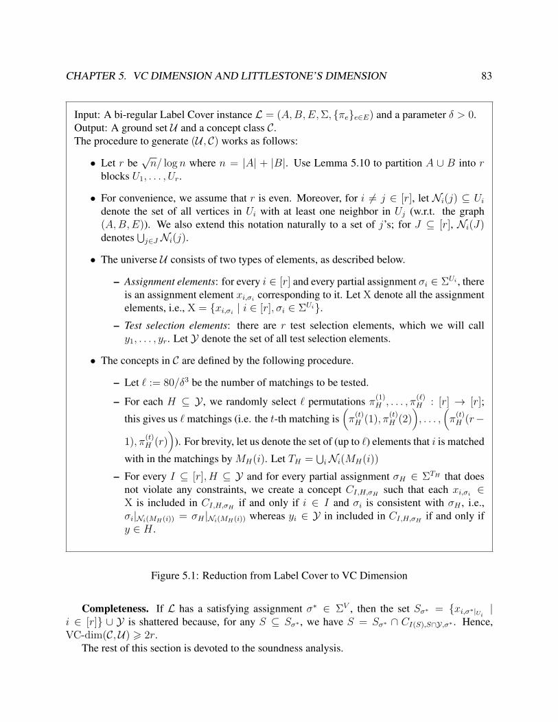
CHAPTER 5. VC DIMENSION AND LITTLESTONE’S DIMENSION 83
Input: A bi-regular Label Cover instance L = (A,B,E,Σ, πee∈E) and a parameter δ > 0.Output: A ground set U and a concept class C.The procedure to generate (U , C) works as follows:
• Let r be√n/ log n where n = |A| + |B|. Use Lemma 5.10 to partition A ∪ B into r
blocks U1, . . . , Ur.
• For convenience, we assume that r is even. Moreover, for i 6= j ∈ [r], let Ni(j) ⊆ Uidenote the set of all vertices in Ui with at least one neighbor in Uj (w.r.t. the graph(A,B,E)). We also extend this notation naturally to a set of j’s; for J ⊆ [r], Ni(J)denotes
⋃j∈J Ni(j).
• The universe U consists of two types of elements, as described below.
– Assignment elements: for every i ∈ [r] and every partial assignment σi ∈ ΣUi , thereis an assignment element xi,σi corresponding to it. Let X denote all the assignmentelements, i.e., X = xi,σi | i ∈ [r], σi ∈ ΣUi.
– Test selection elements: there are r test selection elements, which we will cally1, . . . , yr. Let Y denote the set of all test selection elements.
• The concepts in C are defined by the following procedure.
– Let ` := 80/δ3 be the number of matchings to be tested.
– For each H ⊆ Y , we randomly select ` permutations π(1)H , . . . , π
(`)H : [r] → [r];
this gives us ` matchings (i.e. the t-th matching is(π
(t)H (1), π(t)
H (2)), . . . ,
(π
(t)H (r−
1), π(t)H (r)
)). For brevity, let us denote the set of (up to `) elements that i is matched
with in the matchings by MH(i). Let TH = ⋃iNi(MH(i))
– For every I ⊆ [r], H ⊆ Y and for every partial assignment σH ∈ ΣTH that doesnot violate any constraints, we create a concept CI,H,σH such that each xi,σi ∈X is included in CI,H,σH if and only if i ∈ I and σi is consistent with σH , i.e.,σi|Ni(MH(i)) = σH |Ni(MH(i)) whereas yi ∈ Y in included in CI,H,σH if and only ify ∈ H .
Figure 5.1: Reduction from Label Cover to VC Dimension
Completeness. If L has a satisfying assignment σ∗ ∈ ΣV , then the set Sσ∗ = xi,σ∗|Ui |i ∈ [r] ∪ Y is shattered because, for any S ⊆ Sσ∗ , we have S = Sσ∗ ∩ CI(S),S∩Y,σ∗ . Hence,VC-dim(C,U) > 2r.
The rest of this section is devoted to the soundness analysis.
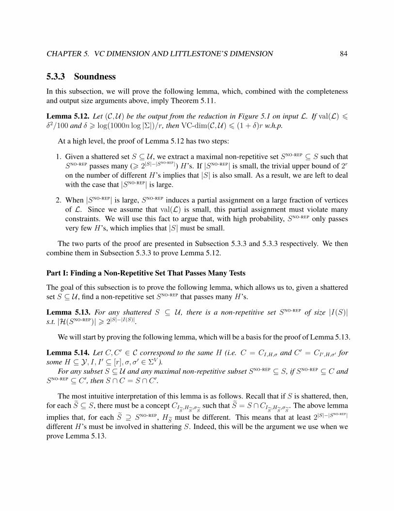
CHAPTER 5. VC DIMENSION AND LITTLESTONE’S DIMENSION 84
5.3.3 SoundnessIn this subsection, we will prove the following lemma, which, combined with the completenessand output size arguments above, imply Theorem 5.11.
Lemma 5.12. Let (C,U) be the output from the reduction in Figure 5.1 on input L. If val(L) 6δ2/100 and δ > log(1000n log |Σ|)/r, then VC-dim(C,U) 6 (1 + δ)r w.h.p.
At a high level, the proof of Lemma 5.12 has two steps:
1. Given a shattered set S ⊆ U , we extract a maximal non-repetitive set SNO-REP ⊆ S such thatSNO-REP passes many (> 2|S|−|SNO-REP|) H’s. If |SNO-REP| is small, the trivial upper bound of 2ron the number of different H’s implies that |S| is also small. As a result, we are left to dealwith the case that |SNO-REP| is large.
2. When |SNO-REP| is large, SNO-REP induces a partial assignment on a large fraction of verticesof L. Since we assume that val(L) is small, this partial assignment must violate manyconstraints. We will use this fact to argue that, with high probability, SNO-REP only passesvery few H’s, which implies that |S| must be small.
The two parts of the proof are presented in Subsection 5.3.3 and 5.3.3 respectively. We thencombine them in Subsection 5.3.3 to prove Lemma 5.12.
Part I: Finding a Non-Repetitive Set That Passes Many Tests
The goal of this subsection is to prove the following lemma, which allows us to, given a shatteredset S ⊆ U , find a non-repetitive set SNO-REP that passes many H’s.
Lemma 5.13. For any shattered S ⊆ U , there is a non-repetitive set SNO-REP of size |I(S)|s.t. |H(SNO-REP)| > 2|S|−|I(S)|.
We will start by proving the following lemma, which will be a basis for the proof of Lemma 5.13.
Lemma 5.14. Let C,C ′ ∈ C correspond to the same H (i.e. C = CI,H,σ and C ′ = CI′,H,σ′ forsome H ⊆ Y , I, I ′ ⊆ [r], σ, σ′ ∈ ΣV ).
For any subset S ⊆ U and any maximal non-repetitive subset SNO-REP ⊆ S, if SNO-REP ⊆ C andSNO-REP ⊆ C ′, then S ∩ C = S ∩ C ′.
The most intuitive interpretation of this lemma is as follows. Recall that if S is shattered, then,for each S ⊆ S, there must be a concept CI
S,HS,σS
such that S = S ∩CIS,HS,σS. The above lemma
implies that, for each S ⊇ SNO-REP, HS
must be different. This means that at least 2|S|−|SNO-REP|
different H’s must be involved in shattering S. Indeed, this will be the argument we use when weprove Lemma 5.13.
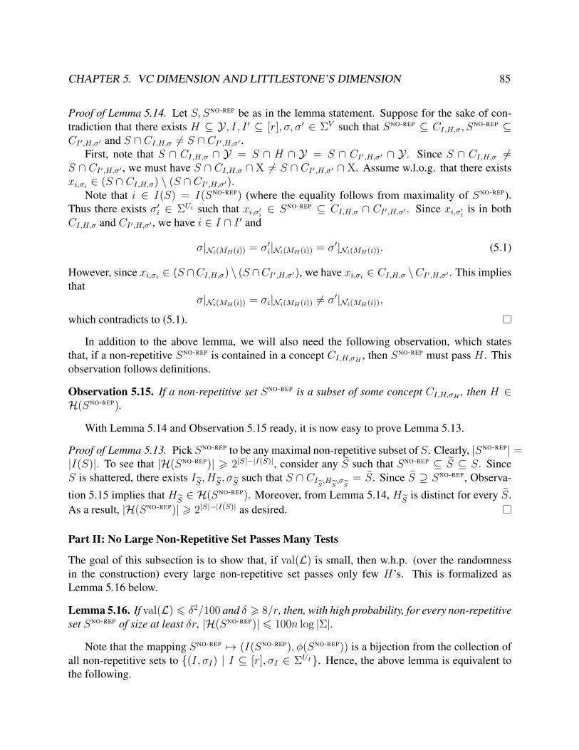
CHAPTER 5. VC DIMENSION AND LITTLESTONE’S DIMENSION 85
Proof of Lemma 5.14. Let S, SNO-REP be as in the lemma statement. Suppose for the sake of con-tradiction that there exists H ⊆ Y , I, I ′ ⊆ [r], σ, σ′ ∈ ΣV such that SNO-REP ⊆ CI,H,σ, S
NO-REP ⊆CI′,H,σ′ and S ∩ CI,H,σ 6= S ∩ CI′,H,σ′ .
First, note that S ∩ CI,H,σ ∩ Y = S ∩ H ∩ Y = S ∩ CI′,H,σ′ ∩ Y . Since S ∩ CI,H,σ 6=S ∩ CI′,H,σ′ , we must have S ∩ CI,H,σ ∩ X 6= S ∩ CI′,H,σ′ ∩ X. Assume w.l.o.g. that there existsxi,σi ∈ (S ∩ CI,H,σ) \ (S ∩ CI′,H,σ′).
Note that i ∈ I(S) = I(SNO-REP) (where the equality follows from maximality of SNO-REP).Thus there exists σ′i ∈ ΣUi such that xi,σ′i ∈ SNO-REP ⊆ CI,H,σ ∩ CI′,H,σ′ . Since xi,σ′i is in bothCI,H,σ and CI′,H,σ′ , we have i ∈ I ∩ I ′ and
σ|Ni(MH(i)) = σ′i|Ni(MH(i)) = σ′|Ni(MH(i)). (5.1)
However, since xi,σi ∈ (S ∩CI,H,σ) \ (S ∩CI′,H,σ′), we have xi,σi ∈ CI,H,σ \CI′,H,σ′ . This impliesthat
σ|Ni(MH(i)) = σi|Ni(MH(i)) 6= σ′|Ni(MH(i)),
which contradicts to (5.1).
In addition to the above lemma, we will also need the following observation, which statesthat, if a non-repetitive SNO-REP is contained in a concept CI,H,σH , then SNO-REP must pass H . Thisobservation follows definitions.
Observation 5.15. If a non-repetitive set SNO-REP is a subset of some concept CI,H,σH , then H ∈H(SNO-REP).
With Lemma 5.14 and Observation 5.15 ready, it is now easy to prove Lemma 5.13.
Proof of Lemma 5.13. Pick SNO-REP to be any maximal non-repetitive subset of S. Clearly, |SNO-REP| =|I(S)|. To see that |H(SNO-REP)| > 2|S|−|I(S)|, consider any S such that SNO-REP ⊆ S ⊆ S. SinceS is shattered, there exists I
S, H
S, σ
Ssuch that S ∩ CI
S,HS,σS
= S. Since S ⊇ SNO-REP, Observa-
tion 5.15 implies that HS∈ H(SNO-REP). Moreover, from Lemma 5.14, H
Sis distinct for every S.
As a result, |H(SNO-REP)| > 2|S|−|I(S)| as desired.
Part II: No Large Non-Repetitive Set Passes Many Tests
The goal of this subsection is to show that, if val(L) is small, then w.h.p. (over the randomnessin the construction) every large non-repetitive set passes only few H’s. This is formalized asLemma 5.16 below.
Lemma 5.16. If val(L) 6 δ2/100 and δ > 8/r, then, with high probability, for every non-repetitiveset SNO-REP of size at least δr, |H(SNO-REP)| 6 100n log |Σ|.
Note that the mapping SNO-REP 7→ (I(SNO-REP), φ(SNO-REP)) is a bijection from the collection ofall non-repetitive sets to (I, σI) | I ⊆ [r], σI ∈ ΣUI. Hence, the above lemma is equivalent tothe following.
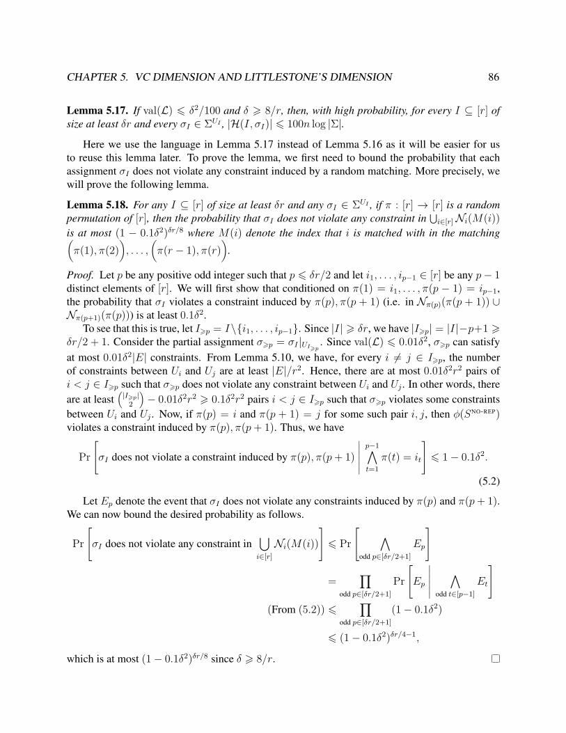
CHAPTER 5. VC DIMENSION AND LITTLESTONE’S DIMENSION 86
Lemma 5.17. If val(L) 6 δ2/100 and δ > 8/r, then, with high probability, for every I ⊆ [r] ofsize at least δr and every σI ∈ ΣUI , |H(I, σI)| 6 100n log |Σ|.
Here we use the language in Lemma 5.17 instead of Lemma 5.16 as it will be easier for usto reuse this lemma later. To prove the lemma, we first need to bound the probability that eachassignment σI does not violate any constraint induced by a random matching. More precisely, wewill prove the following lemma.
Lemma 5.18. For any I ⊆ [r] of size at least δr and any σI ∈ ΣUI , if π : [r] → [r] is a randompermutation of [r], then the probability that σI does not violate any constraint in
⋃i∈[r]Ni(M(i))
is at most (1 − 0.1δ2)δr/8 where M(i) denote the index that i is matched with in the matching(π(1), π(2)
), . . . ,
(π(r − 1), π(r)
).
Proof. Let p be any positive odd integer such that p 6 δr/2 and let i1, . . . , ip−1 ∈ [r] be any p− 1distinct elements of [r]. We will first show that conditioned on π(1) = i1, . . . , π(p − 1) = ip−1,the probability that σI violates a constraint induced by π(p), π(p + 1) (i.e. in Nπ(p)(π(p + 1)) ∪Nπ(p+1)(π(p))) is at least 0.1δ2.
To see that this is true, let I>p = I\i1, . . . , ip−1. Since |I| > δr, we have |I>p| = |I|−p+1 >δr/2 + 1. Consider the partial assignment σ>p = σI |UI>p . Since val(L) 6 0.01δ2, σ>p can satisfyat most 0.01δ2|E| constraints. From Lemma 5.10, we have, for every i 6= j ∈ I>p, the numberof constraints between Ui and Uj are at least |E|/r2. Hence, there are at most 0.01δ2r2 pairs ofi < j ∈ I>p such that σ>p does not violate any constraint between Ui and Uj . In other words, thereare at least
(|I>p|
2
)− 0.01δ2r2 > 0.1δ2r2 pairs i < j ∈ I>p such that σ>p violates some constraints
between Ui and Uj . Now, if π(p) = i and π(p + 1) = j for some such pair i, j, then φ(SNO-REP)violates a constraint induced by π(p), π(p+ 1). Thus, we have
PrσI does not violate a constraint induced by π(p), π(p+ 1)
∣∣∣∣∣∣p−1∧t=1
π(t) = it
6 1− 0.1δ2.
(5.2)
Let Ep denote the event that σI does not violate any constraints induced by π(p) and π(p+ 1).We can now bound the desired probability as follows.
PrσI does not violate any constraint in
⋃i∈[r]Ni(M(i))
6 Pr ∧
odd p∈[δr/2+1]Ep
=
∏odd p∈[δr/2+1]
PrEp
∣∣∣∣∣∣∧
odd t∈[p−1]Et
(From (5.2)) 6
∏odd p∈[δr/2+1]
(1− 0.1δ2)
6 (1− 0.1δ2)δr/4−1,
which is at most (1− 0.1δ2)δr/8 since δ > 8/r.
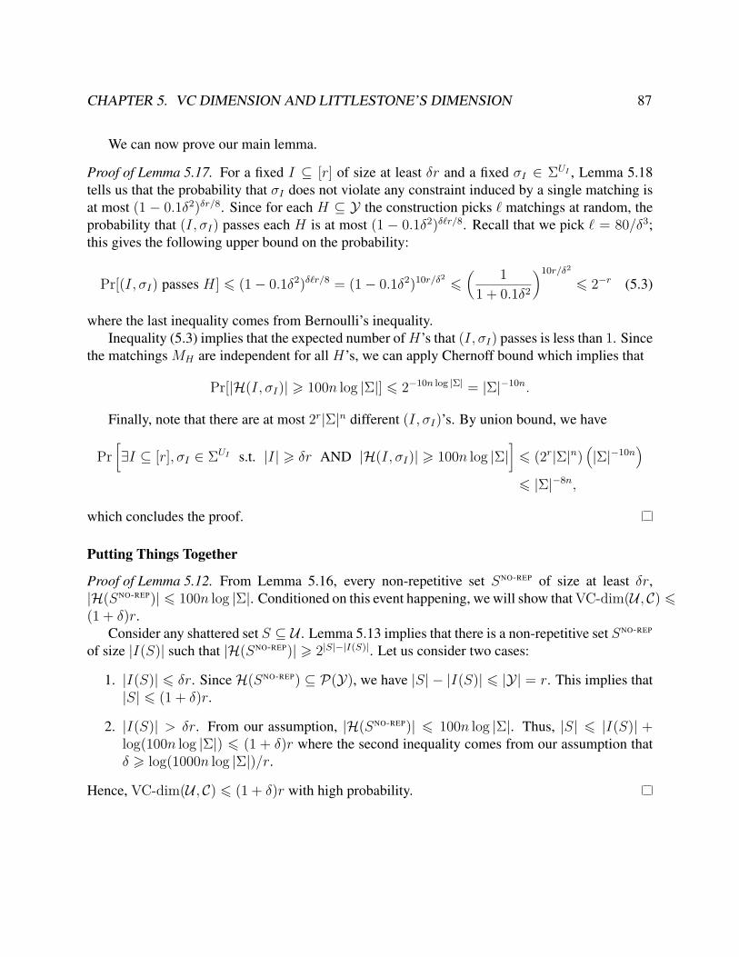
CHAPTER 5. VC DIMENSION AND LITTLESTONE’S DIMENSION 87
We can now prove our main lemma.
Proof of Lemma 5.17. For a fixed I ⊆ [r] of size at least δr and a fixed σI ∈ ΣUI , Lemma 5.18tells us that the probability that σI does not violate any constraint induced by a single matching isat most (1 − 0.1δ2)δr/8. Since for each H ⊆ Y the construction picks ` matchings at random, theprobability that (I, σI) passes each H is at most (1 − 0.1δ2)δ`r/8. Recall that we pick ` = 80/δ3;this gives the following upper bound on the probability:
Pr[(I, σI) passes H] 6 (1− 0.1δ2)δ`r/8 = (1− 0.1δ2)10r/δ26( 1
1 + 0.1δ2
)10r/δ2
6 2−r (5.3)
where the last inequality comes from Bernoulli’s inequality.Inequality (5.3) implies that the expected number ofH’s that (I, σI) passes is less than 1. Since
the matchings MH are independent for all H’s, we can apply Chernoff bound which implies that
Pr[|H(I, σI)| > 100n log |Σ|] 6 2−10n log |Σ| = |Σ|−10n.
Finally, note that there are at most 2r|Σ|n different (I, σI)’s. By union bound, we have
Pr[∃I ⊆ [r], σI ∈ ΣUI s.t. |I| > δr AND |H(I, σI)| > 100n log |Σ|
]6 (2r|Σ|n)
(|Σ|−10n
)6 |Σ|−8n,
which concludes the proof.
Putting Things Together
Proof of Lemma 5.12. From Lemma 5.16, every non-repetitive set SNO-REP of size at least δr,|H(SNO-REP)| 6 100n log |Σ|. Conditioned on this event happening, we will show that VC-dim(U , C) 6(1 + δ)r.
Consider any shattered set S ⊆ U . Lemma 5.13 implies that there is a non-repetitive set SNO-REP
of size |I(S)| such that |H(SNO-REP)| > 2|S|−|I(S)|. Let us consider two cases:
1. |I(S)| 6 δr. Since H(SNO-REP) ⊆ P(Y), we have |S| − |I(S)| 6 |Y| = r. This implies that|S| 6 (1 + δ)r.
2. |I(S)| > δr. From our assumption, |H(SNO-REP)| 6 100n log |Σ|. Thus, |S| 6 |I(S)| +log(100n log |Σ|) 6 (1 + δ)r where the second inequality comes from our assumption thatδ > log(1000n log |Σ|)/r.
Hence, VC-dim(U , C) 6 (1 + δ)r with high probability.
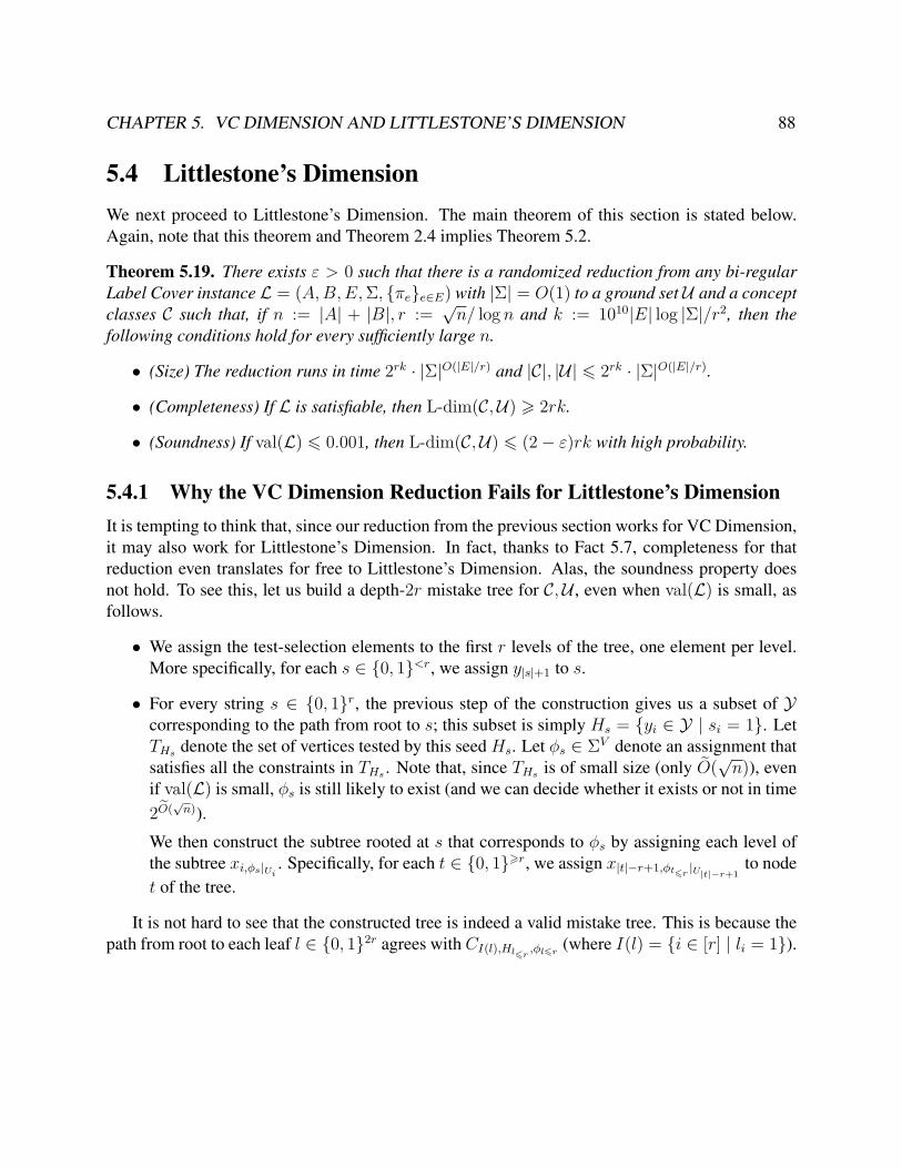
CHAPTER 5. VC DIMENSION AND LITTLESTONE’S DIMENSION 88
5.4 Littlestone’s DimensionWe next proceed to Littlestone’s Dimension. The main theorem of this section is stated below.Again, note that this theorem and Theorem 2.4 implies Theorem 5.2.
Theorem 5.19. There exists ε > 0 such that there is a randomized reduction from any bi-regularLabel Cover instance L = (A,B,E,Σ, πee∈E) with |Σ| = O(1) to a ground set U and a conceptclasses C such that, if n := |A| + |B|, r :=
√n/ log n and k := 1010|E| log |Σ|/r2, then the
following conditions hold for every sufficiently large n.
• (Size) The reduction runs in time 2rk · |Σ|O(|E|/r) and |C|, |U| 6 2rk · |Σ|O(|E|/r).
• (Completeness) If L is satisfiable, then L-dim(C,U) > 2rk.
• (Soundness) If val(L) 6 0.001, then L-dim(C,U) 6 (2− ε)rk with high probability.
5.4.1 Why the VC Dimension Reduction Fails for Littlestone’s DimensionIt is tempting to think that, since our reduction from the previous section works for VC Dimension,it may also work for Littlestone’s Dimension. In fact, thanks to Fact 5.7, completeness for thatreduction even translates for free to Littlestone’s Dimension. Alas, the soundness property doesnot hold. To see this, let us build a depth-2r mistake tree for C,U , even when val(L) is small, asfollows.
• We assign the test-selection elements to the first r levels of the tree, one element per level.More specifically, for each s ∈ 0, 1<r, we assign y|s|+1 to s.
• For every string s ∈ 0, 1r, the previous step of the construction gives us a subset of Ycorresponding to the path from root to s; this subset is simply Hs = yi ∈ Y | si = 1. LetTHs denote the set of vertices tested by this seed Hs. Let φs ∈ ΣV denote an assignment thatsatisfies all the constraints in THs . Note that, since THs is of small size (only O(
√n)), even
if val(L) is small, φs is still likely to exist (and we can decide whether it exists or not in time2O(√n)).
We then construct the subtree rooted at s that corresponds to φs by assigning each level ofthe subtree xi,φs|Ui . Specifically, for each t ∈ 0, 1>r, we assign x|t|−r+1,φt6r |U|t|−r+1
to nodet of the tree.
It is not hard to see that the constructed tree is indeed a valid mistake tree. This is because thepath from root to each leaf l ∈ 0, 12r agrees with CI(l),Hl6r ,φl6r (where I(l) = i ∈ [r] | li = 1).
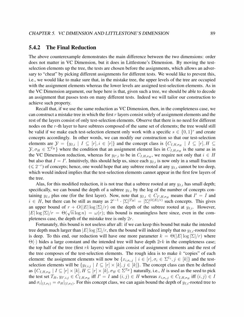
CHAPTER 5. VC DIMENSION AND LITTLESTONE’S DIMENSION 89
5.4.2 The Final ReductionThe above counterexample demonstrates the main difference between the two dimensions: orderdoes not matter in VC Dimension, but it does in Littlestone’s Dimension. By moving the test-selection elements up the tree, the tests are chosen before the assignments, which allows an adver-sary to “cheat” by picking different assignments for different tests. We would like to prevent this,i.e., we would like to make sure that, in the mistake tree, the upper levels of the tree are occupiedwith the assignment elements whereas the lower levels are assigned test-selection elements. As inthe VC Dimension argument, our hope here is that, given such a tree, we should be able to decodean assignment that passes tests on many different tests. Indeed we will tailor our construction toachieve such property.
Recall that, if we use the same reduction as VC Dimension, then, in the completeness case, wecan construct a mistake tree in which the first r layers consist solely of assignment elements and therest of the layers consist of only test-selection elements. Observe that there is no need for differentnodes on the r-th layer to have subtrees composed of the same set of elements; the tree would stillbe valid if we make each test-selection element only work with a specific s ∈ 0, 1r and createconcepts accordingly. In other words, we can modify our construction so that our test-selectionelements are Y = yI,i | I ⊆ [r], i ∈ [r] and the concept class is CI,H,σH | I ⊆ [r], H ⊆Y , σH ∈ ΣTH where the condition that an assignment element lies in CI,H,σH is the same as inthe VC Dimension reduction, whereas for yI′,i to be in CI,H,σH , we require not only that i ∈ Hbut also that I = I ′. Intuitively, this should help us, since each yI,i is now only in a small fraction(6 2−r) of concepts; hence, one would hope that any subtree rooted at any yI,i cannot be too deep,which would indeed implies that the test-selection elements cannot appear in the first few layers ofthe tree.
Alas, for this modified reduction, it is not true that a subtree rooted at any yI,i has small depth;specifically, we can bound the depth of a subtree yI,i by the log of the number of concepts con-taining yI,i plus one (for the first layer). Now, note that yI,i ∈ CI′,H,σH means that I ′ = I andi ∈ H , but there can be still as many as 2r−1 · |Σ||TH | = |Σ|O(|E|/r) such concepts. This givesan upper bound of r + O(|E| log |Σ|/r) on the depth of the subtree rooted at yI,i. However,|E| log |Σ|/r = Θ(
√n log n) = ω(r); this bound is meaningless here since, even in the com-
pleteness case, the depth of the mistake tree is only 2r.Fortunately, this bound is not useless after all: if we can keep this bound but make the intended
tree depth much larger than |E| log |Σ|/r, then the bound will indeed imply that no yI,i-rooted treeis deep. To this end, our reduction will have one more parameter k = Θ(|E| log |Σ|/r) whereΘ(·) hides a large constant and the intended tree will have depth 2rk in the completeness case;the top half of the tree (first rk layers) will again consist of assignment elements and the rest ofthe tree composes of the test-selection elements. The rough idea is to make k “copies” of eachelement: the assignment elements will now be xi,σi,j | i ∈ [r], σi ∈ ΣUi , j ∈ [k] and the test-selection elements will be yI,i,j | I ⊆ [r] × [k], j ∈ [k]. The concept class can then be definedas CI,H,σH | I ⊆ [r]× [k], H ⊆ [r]× [k], σH ∈ ΣTH naturally, i.e., H is used as the seed to pickthe test set TH , yI′,i,j ∈ CI,H,σH iff I ′ = I and (i, j) ∈ H whereas xi,σi,j ∈ CI,H,σH iff (i, j) ∈ Iand σi|(I,σI) = σH |(I,σI). For this concept class, we can again bound the depth of yI,i-rooted tree to
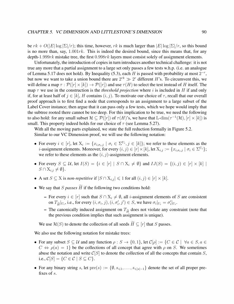
CHAPTER 5. VC DIMENSION AND LITTLESTONE’S DIMENSION 90
be rk + O(|E| log |Σ|/r); this time, however, rk is much larger than |E| log |Σ|/r, so this boundis no more than, say, 1.001rk. This is indeed the desired bound, since this means that, for anydepth-1.999rk mistake tree, the first 0.998rk layers must consist solely of assignment elements.
Unfortunately, the introduction of copies in turn introduces another technical challenge: it is nottrue any more that a partial assignment to a large set only passes a few tests w.h.p. (i.e. an analogueof Lemma 5.17 does not hold). By Inequality (5.3), each H is passed with probability at most 2−r,but now we want to take a union bound there are 2rk 2r different H’s. To circumvent this, wewill define a map τ : P([r]× [k])→ P([r]) and use τ(H) to select the test instead of H itself. Themap τ we use in the construction is the threshold projection where i is included in H if and onlyif, for at least half of j ∈ [k], H contains (i, j). To motivate our choice of τ , recall that our overallproof approach is to first find a node that corresponds to an assignment to a large subset of theLabel Cover instance; then argue that it can pass only a few tests, which we hope would imply thatthe subtree rooted there cannot be too deep. For this implication to be true, we need the followingto also hold: for any small subsetH ⊆ P([r]) of τ(H)’s, we have that L-dim(τ−1(H), [r]× [k]) issmall. This property indeed holds for our choice of τ (see Lemma 5.27).
With all the moving parts explained, we state the full reduction formally in Figure 5.2.Similar to our VC Dimension proof, we will use the following notation:
• For every i ∈ [r], let Xi := xi,σi,j | σi ∈ ΣUi , j ∈ [k]; we refer to these elements as thei-assignment elements. Moreover, for every (i, j) ∈ [r]× [k], let Xi,j := xi,σi,j | σi ∈ ΣUi;we refer to these elements as the (i, j)-assignment elements.
• For every S ⊆ U , let I(S) = i ∈ [r] | S ∩ Xi 6= ∅ and IJ(S) = (i, j) ∈ [r] × [k] |S ∩ Xi,j 6= ∅.
• A set S ⊆ X is non-repetitive if |S ∩ Xi,j| 6 1 for all (i, j) ∈ [r]× [k].
• We say that S passes H if the following two conditions hold:
– For every i ∈ [r] such that S ∩ Xi 6= ∅, all i-assignment elements of S are consistenton T
H|Ui , i.e., for every (i, σi, j), (i, σ′i, j′) ∈ S, we have σi|Ui = σ′i|Ui .
– The canonically induced assignment on TH
does not violate any constraint (note thatthe previous condition implies that such assignment is unique).
We useH(S) to denote the collection of all seeds H ⊆ [r] that S passes.
We also use the following notation for mistake trees:
• For any subset S ⊆ U and any function ρ : S → 0, 1, let C[ρ] := C ∈ C | ∀a ∈ S, a ∈C ⇔ ρ(a) = 1 be the collections of all concept that agree with ρ on S. We sometimesabuse the notation and write C[S] to denote the collection of all the concepts that contain S,i.e., C[S] = C ∈ C | S ⊆ C.
• For any binary string s, let pre(s) := ∅, s61, . . . , s6|s|−1 denote the set of all proper pre-fixes of s.
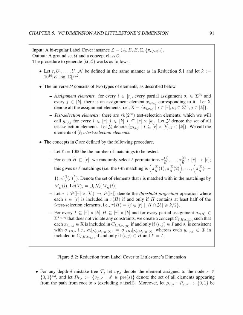
CHAPTER 5. VC DIMENSION AND LITTLESTONE’S DIMENSION 91
Input: A bi-regular Label Cover instance L = (A,B,E,Σ, πee∈E).Output: A ground set U and a concept class C.The procedure to generate (U , C) works as follows:
• Let r, U1, . . . , Ur,N be defined in the same manner as in Reduction 5.1 and let k :=1010|E| log |Σ|/r2.
• The universe U consists of two types of elements, as described below.
– Assignment elements: for every i ∈ [r], every partial assignment σi ∈ ΣUi andevery j ∈ [k], there is an assignment element xi,σi,j corresponding to it. Let Xdenote all the assignment elements, i.e., X = xi,σi,j | i ∈ [r], σi ∈ ΣUi , j ∈ [k].
– Test-selection elements: there are rk(2rk) test-selection elements, which we willcall yI,i,j for every i ∈ [r], j ∈ [k], I ⊆ [r] × [k]. Let Y denote the set of alltest-selection elements. Let Yi denote yI,i,j | I ⊆ [r] × [k], j ∈ [k]. We call theelements of Yi i-test-selection elements.
• The concepts in C are defined by the following procedure.
– Let ` := 1000 be the number of matchings to be tested.
– For each H ⊆ [r], we randomly select ` permutations π(1)H, . . . , π
(`)H
: [r] → [r];
this gives us ` matchings (i.e. the t-th matching is(π
(t)H
(1), π(t)H
(2)), . . . ,
(π
(t)H
(r−
1), π(t)H
(r))
). Denote the set of elements that i is matched with in the matchings by
MH
(i). Let TH
= ⋃iNi(MH
(i))– Let τ : P([r] × [k]) → P([r]) denote the threshold projection operation where
each i ∈ [r] is included in τ(H) if and only if H contains at least half of thei-test-selection elements, i.e., τ(H) = i ∈ [r] | |H ∩ Yi| > k/2.
– For every I ⊆ [r] × [k], H ⊆ [r] × [k] and for every partial assignment στ(H) ∈ΣTτ(H) that does not violate any constraints, we create a conceptCI,H,στ(H) such thateach xi,σi,j ∈ X is included in CI,H,στ(H) if and only if (i, j) ∈ I and σi is consistentwith στ(H), i.e., σi|Ni(Mτ(H)(i)) = στ(H)|Ni(Mτ(H)(i)) whereas each yI′,i,j ∈ Y inincluded in CI,H,στ(H) if and only if (i, j) ∈ H and I ′ = I .
Figure 5.2: Reduction from Label Cover to Littlestone’s Dimension
• For any depth-d mistake tree T , let vT ,s denote the element assigned to the node s ∈0, 16d, and let PT ,s := vT ,s′ | s′ ∈ pre(s) denote the set of all elements appearingfrom the path from root to s (excluding s itself). Moreover, let ρT ,s : PT ,s → 0, 1 be
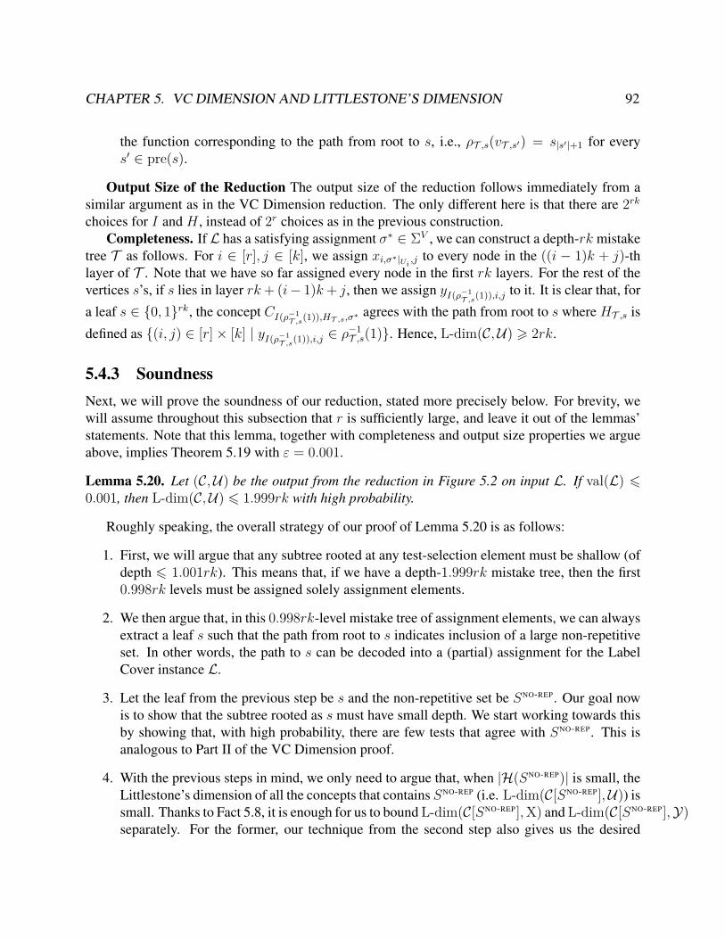
CHAPTER 5. VC DIMENSION AND LITTLESTONE’S DIMENSION 92
the function corresponding to the path from root to s, i.e., ρT ,s(vT ,s′) = s|s′|+1 for everys′ ∈ pre(s).
Output Size of the Reduction The output size of the reduction follows immediately from asimilar argument as in the VC Dimension reduction. The only different here is that there are 2rkchoices for I and H , instead of 2r choices as in the previous construction.
Completeness. If L has a satisfying assignment σ∗ ∈ ΣV , we can construct a depth-rk mistaketree T as follows. For i ∈ [r], j ∈ [k], we assign xi,σ∗|Ui ,j to every node in the ((i − 1)k + j)-thlayer of T . Note that we have so far assigned every node in the first rk layers. For the rest of thevertices s’s, if s lies in layer rk+ (i− 1)k+ j, then we assign yI(ρ−1
T ,s(1)),i,j to it. It is clear that, for
a leaf s ∈ 0, 1rk, the concept CI(ρ−1T ,s(1)),HT ,s,σ∗ agrees with the path from root to s where HT ,s is
defined as (i, j) ∈ [r]× [k] | yI(ρ−1T ,s(1)),i,j ∈ ρ
−1T ,s(1). Hence, L-dim(C,U) > 2rk.
5.4.3 SoundnessNext, we will prove the soundness of our reduction, stated more precisely below. For brevity, wewill assume throughout this subsection that r is sufficiently large, and leave it out of the lemmas’statements. Note that this lemma, together with completeness and output size properties we argueabove, implies Theorem 5.19 with ε = 0.001.
Lemma 5.20. Let (C,U) be the output from the reduction in Figure 5.2 on input L. If val(L) 60.001, then L-dim(C,U) 6 1.999rk with high probability.
Roughly speaking, the overall strategy of our proof of Lemma 5.20 is as follows:
1. First, we will argue that any subtree rooted at any test-selection element must be shallow (ofdepth 6 1.001rk). This means that, if we have a depth-1.999rk mistake tree, then the first0.998rk levels must be assigned solely assignment elements.
2. We then argue that, in this 0.998rk-level mistake tree of assignment elements, we can alwaysextract a leaf s such that the path from root to s indicates inclusion of a large non-repetitiveset. In other words, the path to s can be decoded into a (partial) assignment for the LabelCover instance L.
3. Let the leaf from the previous step be s and the non-repetitive set be SNO-REP. Our goal nowis to show that the subtree rooted as s must have small depth. We start working towards thisby showing that, with high probability, there are few tests that agree with SNO-REP. This isanalogous to Part II of the VC Dimension proof.
4. With the previous steps in mind, we only need to argue that, when |H(SNO-REP)| is small, theLittlestone’s dimension of all the concepts that contains SNO-REP (i.e. L-dim(C[SNO-REP],U)) issmall. Thanks to Fact 5.8, it is enough for us to bound L-dim(C[SNO-REP],X) and L-dim(C[SNO-REP],Y)separately. For the former, our technique from the second step also gives us the desired

CHAPTER 5. VC DIMENSION AND LITTLESTONE’S DIMENSION 93
bound; for the latter, we prove that L-dim(C[SNO-REP],Y) is small by designing an algorithmthat provides correct predictions on a constant fraction of the elements in Y .
Let us now proceed to the details of the proofs.
Part I: Subtree of a Test-Selection Assignment is Shallow
Lemma 5.21. For any yI,i,j ∈ Y , L-dim(C[yI,i,j],U) 6 rk + (4|E|`/r) log |Σ| 6 1.001rk.
Note that the above lemma implies that, in any mistake tree, the depth of the subtree rooted atany vertex s assigned to some yI,i,j ∈ Y is at most 1 + 1.001rk. This is because every concept thatagrees with the path from the root to s must be in C[yI,i,j], which has depth at most 1.001rk.
Proof of Lemma 5.21. Consider any CI′,H,στ(H) ∈ C[yI,i,j],U). Since yI,i,j ∈ CI′,H,στ(H) , wehave I = I ′. Moreover, from Lemma 5.10, we know that
∣∣∣Ni (Mτ(H)(i))∣∣∣ 6 4|E|`/r2, which
implies that |Tτ(H)| 6 4|E|`/r. This means that there are only at most |Σ|4|E|`/r choices of στ(H).Combined with the fact that there are only 2rk choices of H , we have |C[yI,i,j]| 6 2rk · |Σ|4|E|`/r.Fact 5.7 then implies the lemma.
Part II: Deep Mistake Tree Contains a Large Non-Repetitive Set
The goal of this part of the proof is to show that, for mistake tree of X, C of depth slightly less thanrk, there exists a leaf s such that the corresponding path from root to s indicates an inclusion ofa large non-repetitive set; in our notation, this means that we would like to identify a leaf s suchthat IJ(ρ−1
T ,s(1)) is large. Since we will also need a similar bound later in the proof, we will provethe following lemma, which is a generalization of the stated goal that works even for the conceptclass C[SNO-REP] for any non-repetitive SNO-REP. To get back the desired bound, we can simply setSNO-REP = ∅.
Lemma 5.22. For any non-repetitive set SNO-REP and any depth-d mistake tree T of X, C[SNO-REP],there exists a leaf s ∈ 0, 1d such that |IJ(ρ−1
T ,s(1)) \ IJ(SNO-REP)| > d− r.
The proof of this lemma is a double counting argument where we count a specific class ofleaves in two ways, which ultimately leads to the above bound. The leaves that we focus on arethe leaves s ∈ 0, 1d such that, for every (i, j) such that an (i, j)-assignment element appearsin the path from root to s but not in SNO-REP, the first appearance of (i, j)-assignment elementin the path is included. In other words, for every (i, j) ∈ IJ(PT ,s) \ IJ(SNO-REP), if we defineui,j := inf
s′∈pre(s),vT ,s′∈Xi,j|s′|, then sui,j+1 must be equal to 1. We call these leaves the good leaves.
Denote the set of good leaves of T by GT ,SNO-REP .Our first way of counting is the following lemma. Informally, it asserts that different good
leaves agree with different sets H ⊆ [r]. This can be thought of as an analogue of Lemma 5.14in our proof for VC Dimension. Note that this lemma immediately gives an upper bound of 2r on|GT ,SNO-REP |.
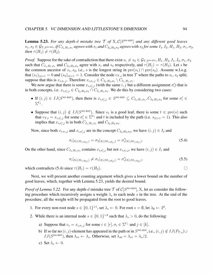
CHAPTER 5. VC DIMENSION AND LITTLESTONE’S DIMENSION 94
Lemma 5.23. For any depth-d mistake tree T of X, C[SNO-REP] and any different good leavess1, s2 ∈ GT ,SNO-REP , ifCI1,H1,σ1 agrees with s1 andCI2,H2,σ2 agrees with s2 for some I1, I2, H1, H2, σ1, σ2,then τ(H1) 6= τ(H2).
Proof. Suppose for the sake of contradiction that there exist s1 6= s2 ∈ GT ,SNO-REP ,H1, H2, I1, I2, σ1, σ2such that CI1,H1,σ1 and CI2,H2,σ2 agree with s1 and s2 respectively, and τ(H1) = τ(H2). Let s bethe common ancestor of s1, s2, i.e., s is the longest string in pre(s1) ∩ pre(s2). Assume w.l.o.g.that (s1)|s|+1 = 0 and (s2)|s|+1 = 1. Consider the node vT ,s in tree T where the paths to s1, s2 split;suppose that this is xi,σi,j . Therefore xi,σi,j ∈ CI2,H2,σ2 \ CI1,H1,σ1 .
We now argue that there is some xi,σ′i,j (with the same i, j but a different assignment σ′i) that isin both concepts, i.e. xi,σ′i,j ∈ CI2,H2,σ2 ∩ CI1,H1,σ1 . We do this by considering two cases:
• If (i, j) ∈ IJ(SNO-REP), then there is xi,σ′i,j ∈ SNO-REP ⊆ CI1,H1,σ1 , CI2,H2,σ2 for some σ′i ∈ΣUi .
• Suppose that (i, j) /∈ IJ(SNO-REP). Since s1 is a good leaf, there is some t ∈ pre(s) suchthat vT ,t = xi,σ′i,j for some σ′i ∈ ΣUi and t is included by the path (i.e. s|t|+1 = 1). This alsoimplies that xi,σ′i,j is in both CI1,H1,σ1 and CI2,H2,σ2 .
Now, since both xi,σi,j and xi,σ′i,j are in the concept CI2,H2,σ2 , we have (i, j) ∈ I2 and
σi|Ni(Mτ(H1)) = σ2|Ni(Mτ(H1)) = σ′i|Ni(Mτ(H1)). (5.4)
On the other hand, since CI1,H1,σ1 contains xi,σ′i,j but not xi,σi,j , we have (i, j) ∈ I1 and
σi|Ni(Mτ(H2)) 6= σ1|Ni(Mτ(H2)) = σ′i|Ni(Mτ(H2)). (5.5)
which contradicts (5.4) since τ(H1) = τ(H2).
Next, we will present another counting argument which gives a lower bound on the number ofgood leaves, which, together with Lemma 5.23, yields the desired bound.
Proof of Lemma 5.22. For any depth-d mistake tree T of C[SNO-REP],X, let us consider the follow-ing procedure which recursively assigns a weight λs to each node s in the tree. At the end of theprocedure, all the weight will be propagated from the root to good leaves.
1. For every non-root node s ∈ 0, 1>1, set λs ← 0. For root s = ∅, let λ∅ ← 2d.
2. While there is an internal node s ∈ 0, 1<d such that λs > 0, do the following:
a) Suppose that vs = xi,σi,j for some i ∈ [r], σi ∈ ΣUi and j ∈ [k].b) If so far no (i, j)-element has appeared in the path or in SNO-REP, i.e., (i, j) /∈ IJ(PT ,s)∪
IJ(SNO-REP), then λs1 ← λs. Otherwise, set λs0 = λs1 = λs/2.
c) Set λs ← 0.
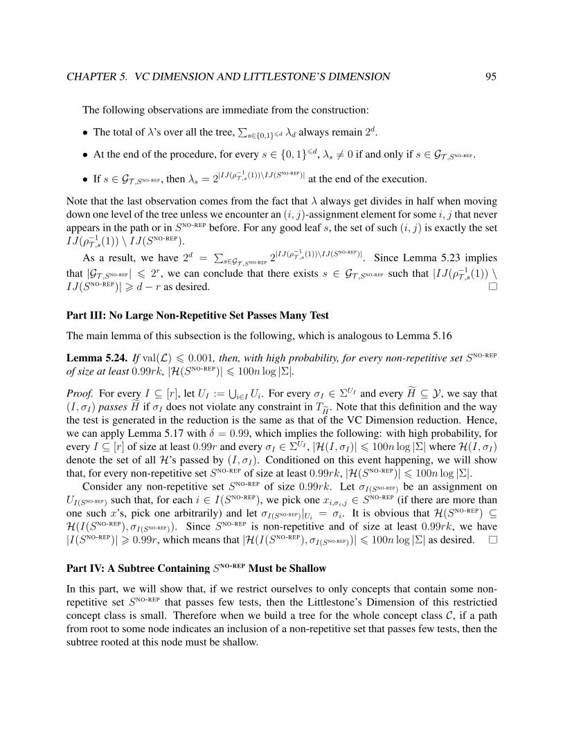
CHAPTER 5. VC DIMENSION AND LITTLESTONE’S DIMENSION 95
The following observations are immediate from the construction:
• The total of λ’s over all the tree,∑s∈0,16d λd always remain 2d.
• At the end of the procedure, for every s ∈ 0, 16d, λs 6= 0 if and only if s ∈ GT ,SNO-REP .
• If s ∈ GT ,SNO-REP , then λs = 2|IJ(ρ−1T ,s(1))\IJ(SNO-REP)| at the end of the execution.
Note that the last observation comes from the fact that λ always get divides in half when movingdown one level of the tree unless we encounter an (i, j)-assignment element for some i, j that neverappears in the path or in SNO-REP before. For any good leaf s, the set of such (i, j) is exactly the setIJ(ρ−1
T ,s(1)) \ IJ(SNO-REP).
As a result, we have 2d = ∑s∈GT ,SNO-REP
2|IJ(ρ−1T ,s(1))\IJ(SNO-REP)|. Since Lemma 5.23 implies
that |GT ,SNO-REP | 6 2r, we can conclude that there exists s ∈ GT ,SNO-REP such that |IJ(ρ−1T ,s(1)) \
IJ(SNO-REP)| > d− r as desired.
Part III: No Large Non-Repetitive Set Passes Many Test
The main lemma of this subsection is the following, which is analogous to Lemma 5.16
Lemma 5.24. If val(L) 6 0.001, then, with high probability, for every non-repetitive set SNO-REP
of size at least 0.99rk, |H(SNO-REP)| 6 100n log |Σ|.
Proof. For every I ⊆ [r], let UI := ⋃i∈I Ui. For every σI ∈ ΣUI and every H ⊆ Y , we say that
(I, σI) passes H if σI does not violate any constraint in TH
. Note that this definition and the waythe test is generated in the reduction is the same as that of the VC Dimension reduction. Hence,we can apply Lemma 5.17 with δ = 0.99, which implies the following: with high probability, forevery I ⊆ [r] of size at least 0.99r and every σI ∈ ΣUI , |H(I, σI)| 6 100n log |Σ| whereH(I, σI)denote the set of all H’s passed by (I, σI). Conditioned on this event happening, we will showthat, for every non-repetitive set SNO-REP of size at least 0.99rk, |H(SNO-REP)| 6 100n log |Σ|.
Consider any non-repetitive set SNO-REP of size 0.99rk. Let σI(SNO-REP) be an assignment onUI(SNO-REP) such that, for each i ∈ I(SNO-REP), we pick one xi,σi,j ∈ SNO-REP (if there are more thanone such x’s, pick one arbitrarily) and let σI(SNO-REP)|Ui = σi. It is obvious that H(SNO-REP) ⊆H(I(SNO-REP), σI(SNO-REP)). Since SNO-REP is non-repetitive and of size at least 0.99rk, we have|I(SNO-REP)| > 0.99r, which means that |H(I(SNO-REP), σI(SNO-REP))| 6 100n log |Σ| as desired.
Part IV: A Subtree Containing SNO-REP Must be Shallow
In this part, we will show that, if we restrict ourselves to only concepts that contain some non-repetitive set SNO-REP that passes few tests, then the Littlestone’s Dimension of this restrictiedconcept class is small. Therefore when we build a tree for the whole concept class C, if a pathfrom root to some node indicates an inclusion of a non-repetitive set that passes few tests, then thesubtree rooted at this node must be shallow.
CHAPTER 5. VC DIMENSION AND LITTLESTONE’S DIMENSION 96
Lemma 5.25. For every non-repetitive set SNO-REP,
L-dim(C[SNO-REP],U) 6 1.75rk − |SNO-REP|+ r + 1000k√r log(|H(SNO-REP)|+ 1).
We prove the above lemma by bounding L-dim(C[SNO-REP],X) and L-dim(C[SNO-REP],Y) sep-arately, and combining them via Fact 5.8. First, we can bound L-dim(C[SNO-REP],X) easily byapplying Lemma 5.22 coupled with the fact that |IJ(SNO-REP)| = |SNO-REP| for every non-repetitiveSNO-REP. This immediately gives the following corollary.
Corollary 5.26. For every non-repetitive set SNO-REP,
L-dim(C[SNO-REP],X) 6 rk − |SNO-REP|+ r.
We will next prove the following bound on L-dim(C[SNO-REP],Y). Note that Corollary 5.26,Lemma 5.27, and Fact 5.8 immediately imply Lemma 5.25.
Lemma 5.27. For every non-repetitive set SNO-REP,
L-dim(C[SNO-REP],Y) 6 0.75rk + 500k√r log(|H(SNO-REP)|+ 1).
The overall outline of the proof of Lemma 5.27 is that we will design a prediction algorithmwhose mistake bound is at most 0.75rk + 1000k
√r log |H(SNO-REP)|. Once we design this algo-
rithm, Lemma 5.6 immediately implies Lemma 5.27. To define our algorithm, we will need thefollowing lemma, which is a general statement that says that, for a small collection of H’s, there isa some H∗ ⊆ [r] that agrees with almost half of every H in the collection.
Lemma 5.28. Let H ⊆ P([r]) be any collections of subsets of [r], there exists H∗ ⊆ [r] suchthat, for every H ∈ H, |H∗∆H| 6 0.5r + 1000
√r log(|H| + 1) where ∆ denotes the symmetric
difference between two sets.
Proof. We use a simple probabilistic method to prove this lemma. Let Hr be a random subsetof [r] (i.e. each i ∈ [r] is included independently with probability 0.5). We will show that, withnon-zero probability, |Hr∆H| 6 0.5r + 1000
√r log(|H|+ 1) for all H ∈ H, which immediately
implies that a desired H∗ exists.Fix H ∈ H. Observe that |Hr∆H| can be written as
∑i∈[r] 1[i ∈ (Hr∆H)]. For each i,
1[i ∈ (Hr∆H)] is a 0, 1 random variable with mean 0.5 independent of other i′ ∈ [r]. ApplyingChernoff bound here yields
Pr[|Hr∆H| > 0.5r + 1000√r log(|H|+ 1)] 6 2− log2(|H|+1) 6
1|H|+ 1 .
Hence, by union bound, we have
Pr[∃H ∈ H, |Hr∆H| > 0.5r + 1000√r log(|H|+ 1)] 6 |H|
|H|+ 1 < 1.
In other words, |Hr∆H| 6 0.5r + 1000√r log(|H|+ 1) for all H ∈ H with non-zero probability
as desired.
CHAPTER 5. VC DIMENSION AND LITTLESTONE’S DIMENSION 97
We also need the following observation, which is an analogue of Observation 5.15 in the VCDimension proof; it follows immediately from definition ofH(S).
Observation 5.29. If a non-repetitive set SNO-REP is a subset of some concept CI,H,στ(H) , thenτ(H) ∈ H(SNO-REP).
With Lemma 5.28 and Observation 5.29 in place, we are now ready to prove Lemma 5.27.
Proof of Lemma 5.27. Let H∗ ⊆ [r] be the set guaranteed by applying Lemma 5.28 with H =H(SNO-REP). Let H∗ := H∗ × [k].
Our prediction algorithm will be very simple: it always predicts according to H∗; i.e., on aninput4 y ∈ Y , it outputs 1[y ∈ H∗]. Consider any sequence (y1, h1), . . . , (yw, hw) that agreeswith a concept CI,H,στ(H) ∈ C[SNO-REP]. Observe that the number of incorrect predictions of ouralgorithm is at most |H∗∆H|.
Since CI,H,στ(H) ∈ C[SNO-REP], Observation 5.29 implies that τ(H) ∈ H(SNO-REP). This meansthat |τ(H)∆H∗| 6 0.5r + 1000
√r log(|H|+ 1). Now, let us consider each i ∈ [r] \ (τ(H)∆H∗).
Suppose that i ∈ τ(H) ∩ H∗. Since i ∈ τ(H), at least k/2 elements of Yi are in H and, sincei ∈ H∗, we have Yi ⊆ H∗. This implies that |(H∗∆H) ∩ Yi| 6 k/2. A similar bound can also bederived when i /∈ τ(H) ∩ H∗. As a result, we have
|H∗∆H| =∑i∈[r]|(H∗∆H) ∩ Yi|
=∑
i∈τ(H)∆H∗|(H∗∆H) ∩ Yi|+
∑i∈[r]\(τ(H)∆H∗)
|(H∗∆H) ∩ Yi|
6 (|τ(H)∆H∗|)(k) + (r − |τ(H)∆H∗|)(k/2)6 0.75rk + 500k
√r log(|H|+ 1),
concluding our proof of Lemma 5.27.
Putting Things Together
Proof of Lemma 5.20. Assume that val(L) 6 0.001. From Lemma 5.24, we know that, with highprobability, |H(SNO-REP)| 6 100n log |Σ| for every non-repetitive set SNO-REP of size at least 0.99rk.Conditioned on this event, we will show that L-dim(C,U) 6 1.999rk.
Suppose for the sake of contradiction that L-dim(C,U) > 1.999rk. Consider any depth-1.999rk mistake tree T of C,U . From Lemma 5.21, no test-selection element is assigned to anynode in the first 1.999rk − 1.001rk − 1 > 0.997rk levels. In other words, the tree induced by thefirst 0.997rk levels is simply a mistake tree of C,X. By Lemma 5.22 with SNO-REP = ∅, there existss ∈ 0, 10.997rk such that |IJ(ρ−1
T ,s(1))| > 0.997rk − r > 0.996rk.4We assume w.l.o.g. that input elements are distinct; if an element appears multiple times, we know the correct
answer from its first appearance and can always correctly predict it afterwards.
CHAPTER 5. VC DIMENSION AND LITTLESTONE’S DIMENSION 98
Since |IJ(ρ−1T ,s(1))| > 0.996rk, there exists a non-repetitive set SNO-REP ⊆ ρ−1
T ,s(1) of size0.996rk. Consider the subtree rooted at s. This is a mistake tree of C[ρT ,s],U of depth 1.002rk.Since SNO-REP ⊆ ρ−1
T ,s(1), we have C[ρT ,s] ⊆ C[SNO-REP]. However, this implies
1.002rk 6 L-dim(C[ρT ,s],U)6 L-dim(C[SNO-REP],U)
(From Lemma 5.25) 6 1.75rk − 0.996rk + r + 100k√r log(|H(SNO-REP)|+ 1)
(From Lemma 5.24) 6 0.754rk + r + 100k√r log(100n log |Σ|+ 1)
= 0.754rk + o(rk),
which is a contradiction when r is sufficiently large.
5.4.4 Quasi-polynomial Algorithm for Littlestone’s DimensionIn this section, we provides the following algorithm which decides whether L-dim(C,U) 6 d intime O(|C| · (2|U|)d). Since we know that L-dim(C,U) 6 log |C|, we can run this algorithm for alld 6 log |C| and compute Littlestone’s Dimension of C,U in quasi-polynomial time.
Theorem 5.30 (Quasi-polynomial Time Algorithm for Littlestone’s Dimension). There is an al-gorithm that, given a universe U , a concept class C and a non-negative integer d, decides whetherL-dim(C,U) 6 d in time O(|C| · (2|U|)d).
Proof. Our algorithm is based on a simple observation: if an element x belongs to at least oneconcept and does not belong to at least one concept, the maximum depth of mistake trees rooted atx is exactly 1 + min L-dim(C[x→ 0],U),L-dim(C[x→ 1],U). Recall from Section 5.4.2 thatC[x → 0] and C[x → 1] denote the collection of concepts that exclude x and the collection ofconcepts that include x respectively.
This yields the following natural recursive algorithm. For each x ∈ U such that C[x →0], C[x→ 1] 6= ∅, recursively run the algorithm on (C[x→ 0],U , d− 1) and (C[x→ 1],U , d− 1).If both executions return NO for some x, then output NO. Otherwise, output YES. When d = 0,there is no need for recursion as we can just check whether |C| 6 1.
Finally, we note that the running time can be easily proved by induction on d.
5.5 Discussion and Open QuestionsIn this work, we prove inapproximability results for VC Dimension and Littlestone’s Dimensionbased on the randomized exponential time hypothesis. Our results provide an almost matchingrunning time lower bound of nlog1−o(1) n for both problems while ruling out approximation ratios of1/2 + o(1) and 1− ε for some ε > 0 for VC Dimension and Littlestone’s Dimension respectively.Even though our results help us gain more insights on approximability of both problems, it isnot yet completely resolved. More specifically, we are not aware of any constant factor no(logn)-time approximation algorithm for either problem; it is an intriguing open question whether such
CHAPTER 5. VC DIMENSION AND LITTLESTONE’S DIMENSION 99
algorithm exists and, if not, whether our reduction can be extended to rule out such algorithm.Another potentially interesting research direction is to derandomize our construction; note that theonly place in the proof in which the randomness is used is in Lemma 5.17.
A related question which remains open, originally posed by Ben-David and Eiron [BE98], isthat of computing the self-directed learning5 mistake bound. Similarly, it may be interesting to un-derstand the complexity of computing (approximating) the recursive teaching dimension [Dol+14;Mor+15].
5Roughly, self-directed learning is similar to the online learning model corresponding to Littlestone’s dimension,but where the learner chooses the order elements; see [BE98] for details.
100
Part II
Parameterized Problems
101
Chapter 6
Inapproximability of k-Dominating Set
In the dominating set problem (DOMSET), we are given an undirected graph G on n vertices andan integer k, and the goal is to decide whether there is a subset of vertices S ⊆ V (G) of size k suchthat every vertex outside S has a neighbor in S (i.e., S dominates every vertex in G and is thuscalled a dominating set). Often regarded as one of the classical problems in computational com-plexity, DOMSET was first shown to be NP-complete in the seminal work of Karp [Kar72]1. Thus,its optimization variant, namely the minimum dominating set, where the goal is to find a dominat-ing set of smallest possible size, is also NP-hard. To circumvent this apparent intractability of theproblem, the study of an approximate version was initiated. The quality of an approximation algo-rithm is measured by the approximation ratio, which is the ratio between the size of the solutionoutput by an algorithm and the size of the minimum dominating set. A simple greedy heuristicfor the problem, which has by now become one of the first approximation algorithms taught inundergraduate and graduate algorithm courses, was intensively studied and was shown to yielda (lnn − ln lnn + Θ(1))-approximation for the problem [Joh74; Chv79; Lov75; Sri95; Sla96].On the opposite side, a long line of works in hardness of approximation [LY94; RS97; Fei98;AMS06; Mos12] culminated in the work of Dinur and Steurer [DS14], who showed that obtaininga (1 − ε) lnn-approximation for the problem is NP-hard for every ε > 0. This essentially settlesthe approximability of the problem.
The parameterized version of DOMSET, which we will refer to simply as k-DOMSET, turnsout to also be intractable: in the same work that introduced the W-hierarchy, Downey and Fel-lows [DF95b] showed that k-DOMSET is complete for the class W[2], which is generally be-lieved to not be contained in FPT. In the ensuing years, stronger running time lower bounds havebeen shown for k-DOMSET under strengthened assumptions. Specifically, Chen et al. [Che+06]ruled out T (k) · no(k)-time algorithm for k-DOMSET assuming ETH. Furthermore, Patrascu andWilliams [PW10] proved, for every k > 2, that, under SETH, not even O(nk−ε) algorithm existsfor k-DOMSET for any ε > 0. Note that the trivial algorithm that enumerates through every k-sizesubset and checks whether it forms a dominating set runs in O(nk+1) time. It is possible to speedup this running time using fast matrix multiplication [EG04; PW10]. In particular, Patrascu and
1To be precise, Karp showed NP-completeness of Set Cover, which is well-known to be equivalent to DOMSET.
CHAPTER 6. INAPPROXIMABILITY OF k-DOMINATING SET 102
Williams [PW10] themselves also gave an nk+o(1)-time algorithm for every k > 7, painting analmost complete picture of the complexity of the problem.
Given the strong negative results for k-DOMSET discussed in the previous paragraph, it isnatural to ask whether we can somehow incorporate the ideas from the area of approximationalgorithms to come up with an FPT approximation algorithm for k-DOMSET. This brings us tothe main question addressed in this chapter: Is there an F (k)-FPT-approximation algorithm fork-DOMSET for some computable function F? This question, which dates back to late 1990s (see,e.g., [DFM06]), has attracted significant attention in literature [DFM06; CGG06; Dow+08; CH10;DF13; HKK13; CHK13; Bon+15; CL16; Cha+17]. In fact, it is even listed in the seminal textbookof Downey and Fellows [DF13] as one of the six “most infamous” open questions2 in the areaof Parameterized Complexity. While earlier attempts fell short of ruling out either F (k) that issuper constant or all FPT algorithms (see Section 6 for more details), the last couple of years haveseen significant progresses on the problem. In a remarkable result of Chen and Lin [CL16], it wasshown that no FPT-approximation for k-DOMSET exists for any constant ratio unless W[1] = FPT.They also proved that, assuming ETH, the inapproximability ratio can be improved to log1/4−ε kfor any constant ε > 0. Very recently, Chalermsook et al. [Cha+17] proved, under GAP-ETH,that k-DOMSET is totally FPT inapproximable, i.e., that no F (k)-approximation algorithm fork-DOMSET exists for any computable function F .
Although Chalermsook et al.’s result on the surface seems to settle the parameterized com-plexity of approximating dominating set, several aspects of the result are somewhat unsatisfactory.First, while GAP-ETH may be plausible, it is quite strong and, in a sense, does much of the workin the proof. Specifically, GAP-ETH itself already gives the gap in hardness of approximation;once there is such a gap, it is not hard3 to build on it and prove other inapproximability results. Asan example, in the analogous situation in NP-hardness of approximation, once one inapproxima-bility result can be shown, others follow via relatively simple gap-preserving reductions (see, e.g.,[PY91]). On the other hand, creating a gap in the first place requires the PCP Theorem [AS98;Aro+98], which involves several new technical ideas such as local checkability of codes and proofcomposition4. Hence, it is desirable to bypass GAP-ETH and prove total FPT inapproximabilityunder assumptions that do not involve hardness of approximation in the first place. Drawing aparallel to the theory of NP-hardness of approximation once again, it is imaginable that a successin bypassing GAP-ETH may also reveal a “PCP-like Theorem” for parameterized complexity.
An additional reason one may wish to bypass GAP-ETH for the total FPT inapproximabil-ity of k-DOMSET is that the latter is a statement purely about parameterized complexity, so oneexpects it to hold under a standard parameterized complexity assumption. Given that Chen and
2Since its publication, two of the questions, the parameterized complexity of k-BICLIQUE [Lin15] and that ofk-EVEN SET (Chapter 10 and [Bon+18]) have been resolved.
3One issue grossed over in this discussion is that of gap amplification. While GAP-ETH gives some constant gap,Chalermsook et al. still needed to amplify the gap to arrive at total FPT inapproximability. Fortunately, unlike theNP-hardness regime that requires Raz’s parallel repetition theorem [Raz98], the gap amplification step in [Cha+17],while non-trivial, only involved relatively simple combinatorial arguments. (See [Cha+17, Theorem 4.3].)
4Even in the “combinatorial proof” of the PCP Theorem [Din07], many of these tools still remain in use, specifi-cally in the alphabet reduction step of the proof.
CHAPTER 6. INAPPROXIMABILITY OF k-DOMINATING SET 103
Lin [CL16] proved W[1]-hardness of approximating k-DOMSET to within any constant factor, aconcrete question here is whether we can show W[1]-hardness of approximation for every functionF (k):
Research Question 1. Can we base the total FPT inapproximability of k-DOMSET on W[1] 6=FPT?
Another issue not completely resolved by [Cha+17] is the running time lower bound. Whilethe work gives a quite strong running time lower bound that rules out any T (k) · no(k)-time F (k)-approximation algorithm for any computable functions T and F , it is still possible that, say,an O(n0.5k)-time algorithm can provide a very good (even constant ratio) approximation for k-DOMSET. Given the aforementioned O(nk−ε) running time lower bound for exact algorithms ofk-DOMSET by Patrascu and Williams [PW10], it seems reasonable to ask whether such a lowerbound can also be established for approximation algorithms:
Research Question 2. Is it hard to approximate k-DOMSET in O(nk−ε)-time?
This question has perplexed researchers, as even with the running time of, say, O(nk−0.1), noF (k)-approximation algorithm is known for k-DOMSET for any computable function F .
Our ContributionsOur contributions are twofold. Firstly, at a higher level, we prove parameterized inapproximabiltyresults for k-DOMSET, answering the two aforementioned open questions (and more). Secondly, ata lower level, we demonstrate a connection between communication complexity and parameterizedinapproximability, allowing us to translate running time lower bounds for parameterized problemsinto parameterized hardness of approximation. This latter part of the contribution extends ideasfrom a recent breakthrough of Abboud et al. [ARW17a], who discovered similar connections andused them to establish inapproximability for problems in P. In this subsection, we only focus onthe first part of our contributions. The second part will be discussed in detail in Section 6.1.
Parameterized Inapproximability of Dominating Set
Our first batch of results are the inapproximability results for k-DOMSET under various stan-dard assumptions in parameterized complexity and fine-grained complexity: W[1] 6= FPT, ETH,SETH and the k-SUM Hypothesis. First, we show total inapproximability of k-DOMSET underW[1] 6= FPT. In fact, we show an even stronger5 inapproximation ratio of (log n)1/poly(k):
5Note that the factor of the form (logn)1/poly(k) is stronger than that of the form F (k). To see this, assume that wehave an F (k)-FPT-approximation algorithm for some computable function F . We can turn this into a (logn)1/poly(k)-approximation algorithm by first checking which of the two ratios is smaller. If F (k) is smaller, then just run theF (k)-FPT-approximation algorithm. Otherwise, use brute force search to solve the problem. Since the latter case canonly occur when n 6 exp(F (k)poly(k)), we have that the running time remains FPT.
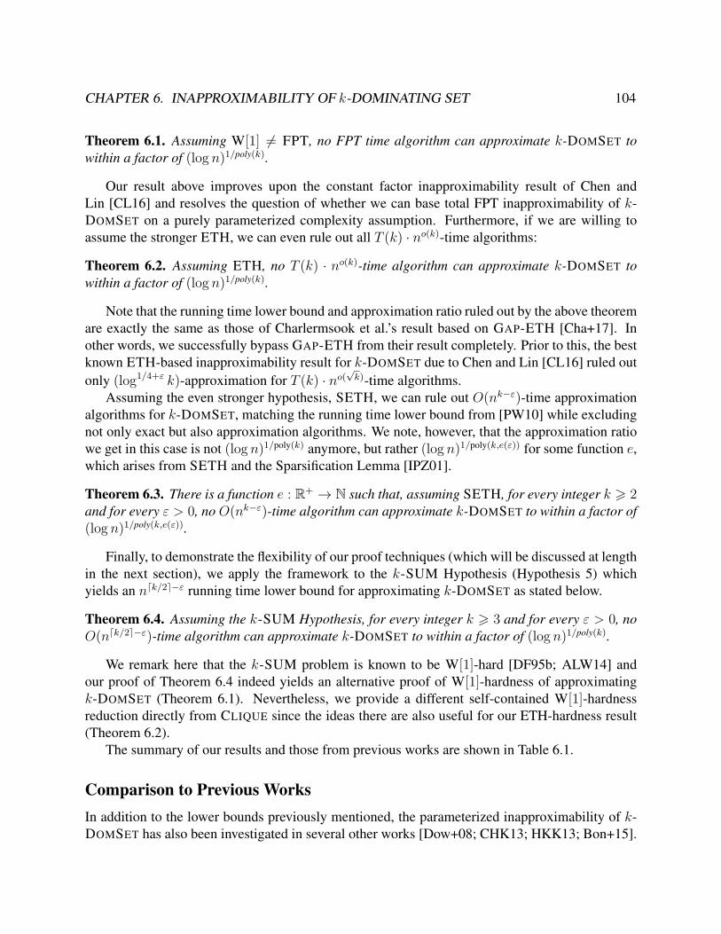
CHAPTER 6. INAPPROXIMABILITY OF k-DOMINATING SET 104
Theorem 6.1. Assuming W[1] 6= FPT, no FPT time algorithm can approximate k-DOMSET towithin a factor of (log n)1/poly(k).
Our result above improves upon the constant factor inapproximability result of Chen andLin [CL16] and resolves the question of whether we can base total FPT inapproximability of k-DOMSET on a purely parameterized complexity assumption. Furthermore, if we are willing toassume the stronger ETH, we can even rule out all T (k) · no(k)-time algorithms:
Theorem 6.2. Assuming ETH, no T (k) · no(k)-time algorithm can approximate k-DOMSET towithin a factor of (log n)1/poly(k).
Note that the running time lower bound and approximation ratio ruled out by the above theoremare exactly the same as those of Charlermsook et al.’s result based on GAP-ETH [Cha+17]. Inother words, we successfully bypass GAP-ETH from their result completely. Prior to this, the bestknown ETH-based inapproximability result for k-DOMSET due to Chen and Lin [CL16] ruled outonly (log1/4+ε k)-approximation for T (k) · no(
√k)-time algorithms.
Assuming the even stronger hypothesis, SETH, we can rule out O(nk−ε)-time approximationalgorithms for k-DOMSET, matching the running time lower bound from [PW10] while excludingnot only exact but also approximation algorithms. We note, however, that the approximation ratiowe get in this case is not (log n)1/poly(k) anymore, but rather (log n)1/poly(k,e(ε)) for some function e,which arises from SETH and the Sparsification Lemma [IPZ01].
Theorem 6.3. There is a function e : R+ → N such that, assuming SETH, for every integer k > 2and for every ε > 0, no O(nk−ε)-time algorithm can approximate k-DOMSET to within a factor of(log n)1/poly(k,e(ε)).
Finally, to demonstrate the flexibility of our proof techniques (which will be discussed at lengthin the next section), we apply the framework to the k-SUM Hypothesis (Hypothesis 5) whichyields an ndk/2e−ε running time lower bound for approximating k-DOMSET as stated below.
Theorem 6.4. Assuming the k-SUM Hypothesis, for every integer k > 3 and for every ε > 0, noO(ndk/2e−ε)-time algorithm can approximate k-DOMSET to within a factor of (log n)1/poly(k).
We remark here that the k-SUM problem is known to be W[1]-hard [DF95b; ALW14] andour proof of Theorem 6.4 indeed yields an alternative proof of W[1]-hardness of approximatingk-DOMSET (Theorem 6.1). Nevertheless, we provide a different self-contained W[1]-hardnessreduction directly from CLIQUE since the ideas there are also useful for our ETH-hardness result(Theorem 6.2).
The summary of our results and those from previous works are shown in Table 6.1.
Comparison to Previous WorksIn addition to the lower bounds previously mentioned, the parameterized inapproximability of k-DOMSET has also been investigated in several other works [Dow+08; CHK13; HKK13; Bon+15].
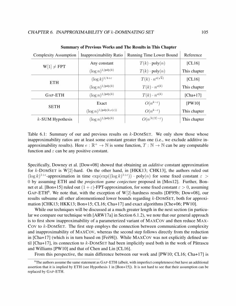
CHAPTER 6. INAPPROXIMABILITY OF k-DOMINATING SET 105
Summary of Previous Works and The Results in This Chapter
Complexity Assumption Inapproximability Ratio Running Time Lower Bound Reference
W[1] 6= FPTAny constant T (k) · poly(n) [CL16]
(log n)1/poly(k) T (k) · poly(n) This chapter
ETH(log k)1/4+ε T (k) · no(
√k) [CL16]
(log n)1/poly(k) T (k) · no(k) This chapter
GAP-ETH (log n)1/poly(k) T (k) · no(k) [Cha+17]
SETHExact O(nk−ε) [PW10]
(log n)1/poly(k,e(ε)) O(nk−ε) This chapter
k-SUM Hypothesis (log n)1/poly(k) O(ndk/2e−ε) This chapter
Table 6.1: Summary of our and previous results on k-DOMSET. We only show those whoseinapproximability ratios are at least some constant greater than one (i.e., we exclude additive in-approximability results). Here e : R+ → N is some function, T : N → N can be any computablefunction and ε can be any positive constant.
Specifically, Downey et al. [Dow+08] showed that obtaining an additive constant approximationfor k-DOMSET is W[2]-hard. On the other hand, in [HKK13; CHK13], the authors ruled out(log k)1+ε-approximation in time exp(exp((log k)1+ε)) · poly(n) for some fixed constant ε >0 by assuming ETH and the projection game conjecture proposed in [Mos12]. Further, Bon-net et al. [Bon+15] ruled out (1 + ε)-FPT-approximation, for some fixed constant ε > 0, assumingGAP-ETH6. We note that, with the exception of W[2]-hardness results [DF95b; Dow+08], ourresults subsume all other aforementioned lower bounds regarding k-DOMSET, both for approxi-mation [CHK13; HKK13; Bon+15; CL16; Cha+17] and exact algorithms [Che+06; PW10].
While our techniques will be discussed at a much greater length in the next section (in particu-lar we compare our technique with [ARW17a] in Section 6.1.2), we note that our general approachis to first show inapproximability of a parameterized variant of MAXCOV and then reduce MAX-COV to k-DOMSET. The first step employs the connection between communication complexityand inapproximability of MAXCOV, whereas the second step follows directly from the reductionin [Cha+17] (which is in turn based on [Fei98]). While MAXCOV was not explicitly defined un-til [Cha+17], its connection to k-DOMSET had been implicitly used both in the work of Patrascuand Williams [PW10] and that of Chen and Lin [CL16].
From this perspective, the main difference between our work and [PW10; CL16; Cha+17] is6The authors assume the same statement as GAP-ETH (albeit, with imperfect completeness) but have an additional
assertion that it is implied by ETH (see Hypothesis 1 in [Bon+15]). It is not hard to see that their assumption can bereplaced by GAP-ETH.
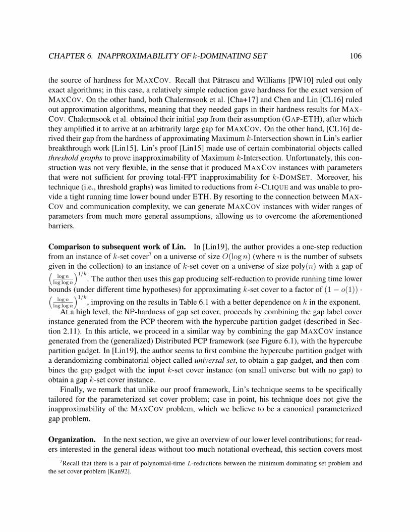
CHAPTER 6. INAPPROXIMABILITY OF k-DOMINATING SET 106
the source of hardness for MAXCOV. Recall that Patrascu and Williams [PW10] ruled out onlyexact algorithms; in this case, a relatively simple reduction gave hardness for the exact version ofMAXCOV. On the other hand, both Chalermsook et al. [Cha+17] and Chen and Lin [CL16] ruledout approximation algorithms, meaning that they needed gaps in their hardness results for MAX-COV. Chalermsook et al. obtained their initial gap from their assumption (GAP-ETH), after whichthey amplified it to arrive at an arbitrarily large gap for MAXCOV. On the other hand, [CL16] de-rived their gap from the hardness of approximating Maximum k-Intersection shown in Lin’s earlierbreakthrough work [Lin15]. Lin’s proof [Lin15] made use of certain combinatorial objects calledthreshold graphs to prove inapproximability of Maximum k-Intersection. Unfortunately, this con-struction was not very flexible, in the sense that it produced MAXCOV instances with parametersthat were not sufficient for proving total-FPT inapproximability for k-DOMSET. Moreover, histechnique (i.e., threshold graphs) was limited to reductions from k-CLIQUE and was unable to pro-vide a tight running time lower bound under ETH. By resorting to the connection between MAX-COV and communication complexity, we can generate MAXCOV instances with wider ranges ofparameters from much more general assumptions, allowing us to overcome the aforementionedbarriers.
Comparison to subsequent work of Lin. In [Lin19], the author provides a one-step reductionfrom an instance of k-set cover7 on a universe of size O(log n) (where n is the number of subsetsgiven in the collection) to an instance of k-set cover on a universe of size poly(n) with a gap of(
lognlog logn
)1/k. The author then uses this gap producing self-reduction to provide running time lower
bounds (under different time hypotheses) for approximating k-set cover to a factor of (1− o(1)) ·(logn
log logn
)1/k, improving on the results in Table 6.1 with a better dependence on k in the exponent.
At a high level, the NP-hardness of gap set cover, proceeds by combining the gap label coverinstance generated from the PCP theorem with the hypercube partition gadget (described in Sec-tion 2.11). In this article, we proceed in a similar way by combining the gap MAXCOV instancegenerated from the (generalized) Distributed PCP framework (see Figure 6.1), with the hypercubepartition gadget. In [Lin19], the author seems to first combine the hypercube partition gadget witha derandomizing combinatorial object called universal set, to obtain a gap gadget, and then com-bines the gap gadget with the input k-set cover instance (on small universe but with no gap) toobtain a gap k-set cover instance.
Finally, we remark that unlike our proof framework, Lin’s technique seems to be specificallytailored for the parameterized set cover problem; case in point, his technique does not give theinapproximability of the MAXCOV problem, which we believe to be a canonical parameterizedgap problem.
Organization. In the next section, we give an overview of our lower level contributions; for read-ers interested in the general ideas without too much notational overhead, this section covers most
7Recall that there is a pair of polynomial-time L-reductions between the minimum dominating set problem andthe set cover problem [Kan92].
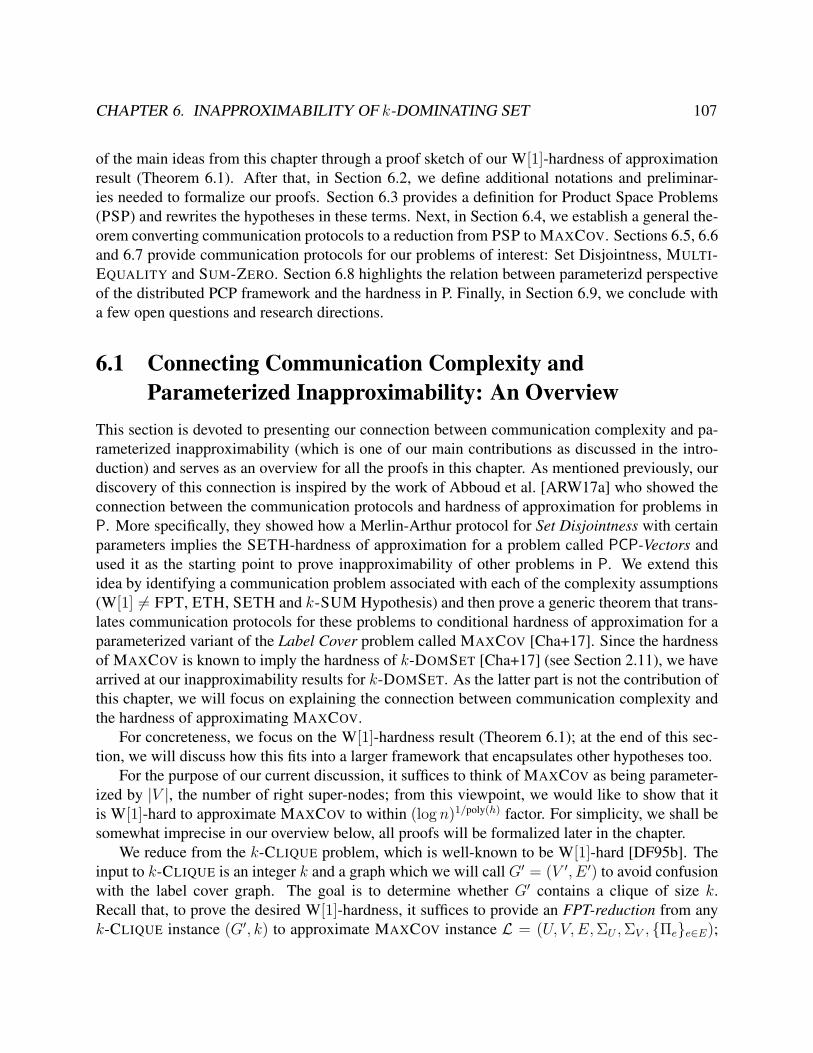
CHAPTER 6. INAPPROXIMABILITY OF k-DOMINATING SET 107
of the main ideas from this chapter through a proof sketch of our W[1]-hardness of approximationresult (Theorem 6.1). After that, in Section 6.2, we define additional notations and preliminar-ies needed to formalize our proofs. Section 6.3 provides a definition for Product Space Problems(PSP) and rewrites the hypotheses in these terms. Next, in Section 6.4, we establish a general the-orem converting communication protocols to a reduction from PSP to MAXCOV. Sections 6.5, 6.6and 6.7 provide communication protocols for our problems of interest: Set Disjointness, MULTI-EQUALITY and SUM-ZERO. Section 6.8 highlights the relation between parameterizd perspectiveof the distributed PCP framework and the hardness in P. Finally, in Section 6.9, we conclude witha few open questions and research directions.
6.1 Connecting Communication Complexity andParameterized Inapproximability: An Overview
This section is devoted to presenting our connection between communication complexity and pa-rameterized inapproximability (which is one of our main contributions as discussed in the intro-duction) and serves as an overview for all the proofs in this chapter. As mentioned previously, ourdiscovery of this connection is inspired by the work of Abboud et al. [ARW17a] who showed theconnection between the communication protocols and hardness of approximation for problems inP. More specifically, they showed how a Merlin-Arthur protocol for Set Disjointness with certainparameters implies the SETH-hardness of approximation for a problem called PCP-Vectors andused it as the starting point to prove inapproximability of other problems in P. We extend thisidea by identifying a communication problem associated with each of the complexity assumptions(W[1] 6= FPT, ETH, SETH and k-SUM Hypothesis) and then prove a generic theorem that trans-lates communication protocols for these problems to conditional hardness of approximation for aparameterized variant of the Label Cover problem called MAXCOV [Cha+17]. Since the hardnessof MAXCOV is known to imply the hardness of k-DOMSET [Cha+17] (see Section 2.11), we havearrived at our inapproximability results for k-DOMSET. As the latter part is not the contribution ofthis chapter, we will focus on explaining the connection between communication complexity andthe hardness of approximating MAXCOV.
For concreteness, we focus on the W[1]-hardness result (Theorem 6.1); at the end of this sec-tion, we will discuss how this fits into a larger framework that encapsulates other hypotheses too.
For the purpose of our current discussion, it suffices to think of MAXCOV as being parameter-ized by |V |, the number of right super-nodes; from this viewpoint, we would like to show that itis W[1]-hard to approximate MAXCOV to within (log n)1/poly(h) factor. For simplicity, we shall besomewhat imprecise in our overview below, all proofs will be formalized later in the chapter.
We reduce from the k-CLIQUE problem, which is well-known to be W[1]-hard [DF95b]. Theinput to k-CLIQUE is an integer k and a graph which we will call G′ = (V ′, E ′) to avoid confusionwith the label cover graph. The goal is to determine whether G′ contains a clique of size k.Recall that, to prove the desired W[1]-hardness, it suffices to provide an FPT-reduction from anyk-CLIQUE instance (G′, k) to approximate MAXCOV instance L = (U, V,E,ΣU ,ΣV , Πee∈E);
CHAPTER 6. INAPPROXIMABILITY OF k-DOMINATING SET 108
this is an FPT-time reduction such that the new parameter |V | is bounded by a function of theoriginal parameter k. Furthermore, since we want a hardness of approximation result for the latter,we will also show that, when (G′, k) is a YES instance of k-CLIQUE, there is a labeling of G thatcovers all the left super-nodes. On the other hand, when (G′, k) is a NO instance of k-CLIQUE, wewish to show that every labeling of G will cover at most 1/(log n)1/poly(h) fraction of the left super-nodes. If we had such a reduction, then we would have arrived at the total FPT-inapproximabilityof MAXCOV under W[1] 6= FPT. But, how would we come up with such a reduction? We will dothis by devising a specific kind of protocol for a communication problem!
6.1.1 A Communication Problem for k-CLIQUE
The communication problem related to k-CLIQUE we consider is a multi-party problem wherethere are h =
(k2
)players, each associated with a two-element subset i, j of [k]. The players
cannot communicate with each other. Rather, there is a referee that they can send messages to.Each player i, j is given two vertices ui,ji and ui,jj such that ui,ji , u
i,jj forms an edge in
G′. The vertices ui,ji and ui,jj are allegedly the i-th and j-th vertices of a clique respectively.The goal is to determine whether there is indeed a k-clique in G′ such that, for every i, j ⊆ [k],ui,ji and ui,jj are the i-th and j-th vertices of the clique.
The communication protocol that we are looking for is a one-round protocol with public ran-domness and by the end of which the referee is the one who outputs the answer. Specifically, theprotocol proceeds as follows. First, the players and the referee together toss r random coins. Then,each player sends an `-bit message to the referee. Finally, the referee decides, based on the mes-sages received and the randomness, either to accept or reject. The protocol is said to have perfectcompleteness and soundness s if (1) when there is a desired clique, the referee always acceptsand (2) when there is no such clique, the referee accepts with probability at most s. The model de-scribed here is referred to in the literature as the multi-party Simultaneous Message Passing (SMP)model [Yao79; Bab+03; FOZ16]. We refer to a protocol in the SMP model as an SMP protocol.
From Communication Protocol to MAXCOV. Before providing a protocol for the previouslydescribed communication problem, let us describe how to turn the protocol into a label coverinstance L = (U, V,E,ΣU ,ΣV , Πee∈E).
• Throughout this chapter, the super graph (U, V,E) is always a complete bipartite graph, i.e.,E = U × V . From this point on, we will drop E from the notation for convenience.
• Let h =(k2
). Again, we associate elements in [h] with two-element subsets of [k]. Each right
super-node represents Player i, j, i.e., V =(
[k]2
). We view each alphabet for super-node
i, j as a possible input to the player, i.e., an edge u, v ∈ E ′ in the graph G′. Assumew.l.o.g. that i < j and u < v. This label represents player i, j receiving u and v as thealleged i-th and j-th vertices of the clique respectively.
CHAPTER 6. INAPPROXIMABILITY OF k-DOMINATING SET 109
• Let U = 0, 1r; that is, we associate left super-node with an r-bit string. For eachγ ∈ 0, 1r, we view each label for the left super-node γ as an accepting configurationon randomness γ, i.e., an h-tuple of `-bit strings (m1,2, . . . ,mk−1,k) ∈ (0, 1`)h suchthat the referee accepts on randomness γ and message m1,2, . . . ,mk−1,k.
• The constraint Πe where e = (γ, i, j) is defined as follows. Recall that each label a of theright super-node i, j corresponds to an input that the player i, j receives in the protocol.For each γ ∈ 0, 1r, suppose that the message produced on this randomness by the i, j-th player on the input corresponding to a is ma,γ . We include in Πe the pair between a andevery accepting configuration on randomness γ that agrees with the message ma,γ . Morespecifically, ((m1,2, . . . ,mk−1,k), a) ∈ Πe iff mi,j = ma,γ .
Consider any right labeling σV . It is not hard to see that, if we run the protocol where the i, j-thplayer is given the edge corresponding σV (i, j) as an input, then the referee accepts a randomstring γ ∈ 0, 1r if and only if the left super-node γ is covered by the labeling S. In other words,the fraction of the left super-nodes covered by S is exactly equal to the acceptance probability ofthe protocol. This means that if (G′, k) is a YES-instance of k-CLIQUE, then we can select σVcorresponding to the edges of a k-clique and every left super-node will be covered. On the otherhand, if (G′, k) is a NO-instance of k-CLIQUE, there is no labeling σV that corresponds to a validk-clique, meaning that every labeling σV covers at most s fraction of the edges. Hence, we haveindeed arrived at hardness of approximation for MAXCOV. Before we move on to describe theprotocol, let us note that the running time of the reduction is poly(2r+`h, |E ′|), which also gives anupper bound on the size of the label cover instance.
SMP Protocol. Observe first that the trivial protocol, one where every player sends the wholeinput to the referee, does not suffice for us; this is because the message length ` is Ω(log n),meaning that the running time of the reduction is nΩ(h) = nΩ(k2) which is not FPT time.
Nevertheless, there still is a simple protocol that does the job. Notice that the input verticesui,ji and ui,jj given to Player i, j are already promised to form an edge. Hence, the only thing
the referee needs to check is whether each alleged vertex of the clique sent to different players arethe same; namely, he only needs to verify that, for every i ∈ [k], we have ui,1i = u
i,2i = · · · =
ui,i−1i = u
i,i+1i = · · · = u
i,ki . In other words, he only needs to check equalities for each of
the k unknowns. The equality problem and its variants are extensively studied in communicationcomplexity (see, e.g., [Yao79; KN97]). In our case, the protocol can be easily derived using anyerror-correcting code. Specifically, for an outcome γ ∈ 0, 1r of the random coin tosses, everyPlayer i, j encodes each of his input (ui,ji and ui,jj ) using a binary error-correcting code andsends only the γ-th bit of each encoded word to the referee. The referee then checks whether, forevery i ∈ [k], the received γ-th bits of the encodings of ui,1i , u
i,2i , . . . , u
i,ki are equal.
In the protocol described above, the message length ` is now only two bits (one bit per vertex),the randomness r used is logarithmic in the block length of the code, the soundness s is one minusthe relative distance of the code. If we use a binary code with constant rate and constant relativedistance (aka good codes), then r will be simply O(log log n); this means that the running time of
CHAPTER 6. INAPPROXIMABILITY OF k-DOMINATING SET 110
the reduction is poly(n, exp(O(k2))) as desired. While the soundness in this case will just be someconstant less than one, we can amplify the soundness by repeating the protocol multiple timesindependently; this increases the randomness and message length, but it is still not hard to see that,with the right number of repetitions, all parameters lie within the desired ranges. With this, wehave completed our sketch for the proof of W[1]-hardness of approximating MAXCOV.
6.1.2 A Framework for Parameterized Hardness of ApproximationThe W[1]-hardness proof sketched above is an example of a much more general connection be-tween communication protocol and the hardness of approximating MAXCOV. To gain insight onthis, consider any function f : X1×· · ·×Xk → 0, 1. This function naturally induces both a com-munication problem and a computational problem. The communication problem for f is one wherethere are k players, each player i receives an input ai ∈ Xi, and they together wish to computef(a1, . . . , ak). The computational problem for f , which we call the Product Space Problem8 of f(abbreviated as PSP(f)), is one where the input consists of subsetsA1 ⊆ X1, . . . , Ak ⊆ Xk and thegoal is to determine whether there exists (a1, . . . , ak) ∈ A1×· · ·×Ak such that f(a1, . . . , ak) = 1.The sketch reduction to MAXCOV above in fact not only applies to the specific communicationproblem of k-CLIQUE: the analogous construction is a generic way to translate any SMP protocolfor the communication problem of any function f to a reduction from PSP(f) to MAXCOV. Tophrase it somewhat differently, if we have an SMP protocol for f with certain parameters andPSP(f) is hard to solve, then MAXCOV is hard to approximate.
This brings us to the framework we use in this chapter. It consists of only two steps. First,we rewrite the problem in the hypotheses as Product Space Problems of some family of functionsF . This gives us the conditional hardness for solving PSP(F). Second, we devise an SMP pro-tocol for every function f ∈ F . Given the connection outlined in the previous paragraph, thisautomatically yields the parameterized hardness of approximating MAXCOV.
To gain more intuition into the framework, note that in the case of k-CLIQUE above, thefunction f ∈ F we consider is just the function f : X1,2 × · · · × Xk,k−1 where each ofX1,2, · · · , Xk,k−1 is a copy of the edge set. The function f “checks” that the edges selectedform a clique, i.e., that, for every i ∈ [k], the alleged i-th vertex of the clique specified in thei, j-coordinate is equal for every j 6= i. Since this is a generalization of the equality function,we call such a class of functions “multi-equality”. It turns out that 3-SAT can also be written asPSP of multi-equality; eachXi contains assignments to 1/k fraction of the clauses and the functionf checks that each variable is assigned the same value across all Xi’s they appear in. A protocolessentially the same as the one given above also works in this setting and immediately gives ourETH-hardness result (Theorem 6.2)! Unfortunately, this does not suffice for our SETH-hardness.In that case, the function used is the k-way set disjointness; this interpretation of SETH is well-known (see, e.g., [Wil05]) and is also used in [ARW17a]. Lastly, the k-SUM problem is alreadywritten in PSP form where f is just the SUM-ZERO function that checks whether the sum of kspecified numbers equals to zero.
8The naming comes from the product structure of the domain of f .
CHAPTER 6. INAPPROXIMABILITY OF k-DOMINATING SET 111
Let us note that in the actual proof, we have to be more careful about the parameters than inthe above sketch. Specifically, the reduction from MAXCOV to k-DOMSET from [Fei98; Cha+17]incurs a blow-up in size that is exponential in terms of the number of vertices in each left super-node (i.e., exponential in |Uγ|). This means that we need |U1|, . . . , |Ur| = o(log n). In the contextof communication protocol, this translates to keeping the message length O(log log n) where O(·)hides a sufficiently small constant. Nevertheless, for the protocol for k-CLIQUE reduction (andmore generally for multi-equality), this does not pose a problem for us since the message lengthbefore repetitions is O(1) bits; we can make sure that we apply only O(log log n) repetitions to theprotocol.
For SUM-ZERO, known protocols either violate the above requirement on message length [Nis94]or use too much randomness [Vio15]. Nonetheless, a simple observation allows us to composeNisan’s protocol [Nis94] and Viola’s protocol [Vio15] and arrive at a protocol with the best of bothparameters. This new protocol may also be of independent interest beyond the scope of our work.
On the other hand, well-known communication complexity lower bounds on set disjointness [Raz92;KS92; Bar+04] rule out the existence of protocols with parameters we wish to have! [ARW17a]also ran into this issue; in our language, they got around this problem by allowing the referee toreceive an advice. This will also be the route we take. Even with advice, however, devising aprotocol with the desired parameters is a technically challenging issue. In particular, until very re-cently, no protocol for set disjointness with O(log log n) message length (and o(n) advice length)was known. This was overcome in the work of Rubinstein [Rub18] who used algebraic geometriccodes to give such a protocol for the two-player case. We extend his protocol in a straightforwardmanner to the k-player case; this extension was also suggested to us by Rubinstein [Rub17a].
A diagram illustrating the overview of our approach can be found in Figure 6.1.
Comparison to Abboud et al. The main result of Abboud et al. [ARW17a] is their SETH-hardness of the gap label cover problem which they refer to as the PCP-Vectors problem. In fact,PCP-Vectors is equivalent to MAXCOV when h = 2 (i.e., the number of right super nodes is two).However, formulating the label cover problem as MAXCOV instead of PCP-Vectors is beneficialfor us, as our goal it to reduce to graph problems.
In their work, they merge the roles of the referee and the first player as it is necessary to achievethe goal of proving hardness of approximation for important problems in P (which are usuallydefined on one or two sets of vectors). However, by doing this the details of the proof becomea little convoluted. On the contrary, our framework with the SMP model is arguably a cleanerframework to work with and it works well for our goal of proving hardness of approximation forparameterized problems.
Finally, we note that our observation that the hardness of approximating MAXCOV can beobtained from any arbitrary hypothesis as long as there is an underlying product structure (asformalized via PSPs) is a new contribution of this chapter.
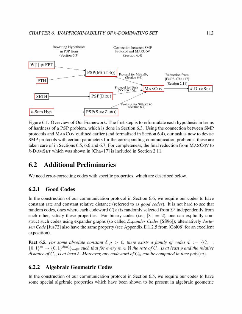
CHAPTER 6. INAPPROXIMABILITY OF k-DOMINATING SET 112
W[1] 6= FPT
ETH
SETH
k-Sum Hyp.
PSP(MULTEQ)
PSP(DISJ)
PSP(SUMZERO)
MAXCOV k-DOMSET
Rewriting Hypothesesin PSP form(Section 6.3)
Connection between SMPProtocol and MAXCOV
(Section 6.4)
Protocol for MULTEQ(Section 6.6)
Protocol for DISJ(Section 6.5)
Protocol for SUMZERO(Section 6.7)
Reduction from[Fei98; Cha+17](Section 2.11)
Figure 6.1: Overview of Our Framework. The first step is to reformulate each hypothesis in termsof hardness of a PSP problem, which is done in Section 6.3. Using the connection between SMPprotocols and MAXCOV outlined earlier (and formalized in Section 6.4), our task is now to deviseSMP protocols with certain parameters for the corresponding communication problems; these aretaken care of in Sections 6.5, 6.6 and 6.7. For completeness, the final reduction from MAXCOV tok-DOMSET which was shown in [Cha+17] is included in Section 2.11.
6.2 Additional PreliminariesWe need error-correcting codes with specific properties, which are described below.
6.2.1 Good CodesIn the construction of our communication protocol in Section 6.6, we require our codes to haveconstant rate and constant relative distance (referred to as good codes). It is not hard to see thatrandom codes, ones where each codeword C(x) is randomly selected from Σd independently fromeach other, satisfy these properties. For binary codes (i.e., |Σ| = 2), one can explicitly con-struct such codes using expander graphs (so called Expander Codes [SS96]); alternatively Juste-sen Code [Jus72] also have the same property (see Appendix E.1.2.5 from [Gol08] for an excellentexposition).
Fact 6.5. For some absolute constant δ, ρ > 0, there exists a family of codes C := Cm :0, 1m → 0, 1d(m)m∈N such that for every m ∈ N the rate of Cm is at least ρ and the relativedistance of Cm is at least δ. Moreover, any codeword of Cm can be computed in time poly(m).
6.2.2 Algebraic Geometric CodesIn the construction of our communication protocol in Section 6.5, we require our codes to havesome special algebraic properties which have been shown to be present in algebraic geometric
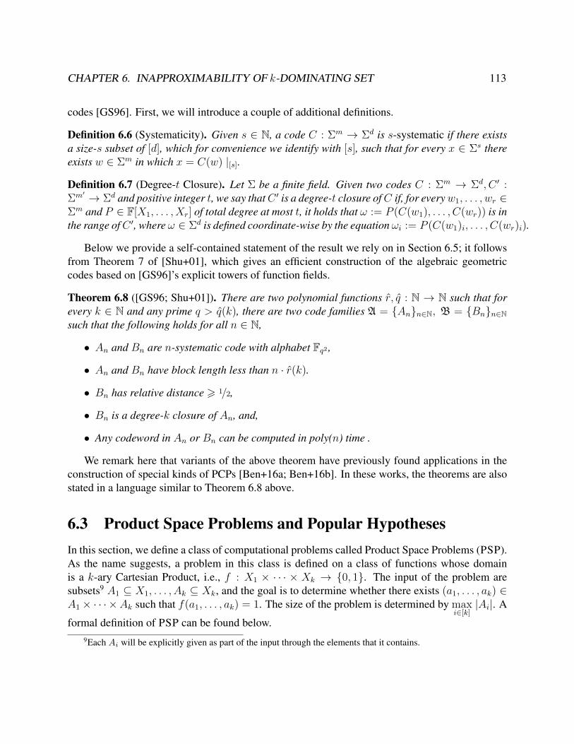
CHAPTER 6. INAPPROXIMABILITY OF k-DOMINATING SET 113
codes [GS96]. First, we will introduce a couple of additional definitions.
Definition 6.6 (Systematicity). Given s ∈ N, a code C : Σm → Σd is s-systematic if there existsa size-s subset of [d], which for convenience we identify with [s], such that for every x ∈ Σs thereexists w ∈ Σm in which x = C(w) |[s].
Definition 6.7 (Degree-t Closure). Let Σ be a finite field. Given two codes C : Σm → Σd, C ′ :Σm′ → Σd and positive integer t, we say thatC ′ is a degree-t closure ofC if, for everyw1, . . . , wr ∈Σm and P ∈ F[X1, . . . , Xr] of total degree at most t, it holds that ω := P (C(w1), . . . , C(wr)) is inthe range ofC ′, where ω ∈ Σd is defined coordinate-wise by the equation ωi := P (C(w1)i, . . . , C(wr)i).
Below we provide a self-contained statement of the result we rely on in Section 6.5; it followsfrom Theorem 7 of [Shu+01], which gives an efficient construction of the algebraic geometriccodes based on [GS96]’s explicit towers of function fields.
Theorem 6.8 ([GS96; Shu+01]). There are two polynomial functions r, q : N → N such that forevery k ∈ N and any prime q > q(k), there are two code families A = Ann∈N, B = Bnn∈Nsuch that the following holds for all n ∈ N,
• An and Bn are n-systematic code with alphabet Fq2 ,
• An and Bn have block length less than n · r(k).
• Bn has relative distance > 1/2,
• Bn is a degree-k closure of An, and,
• Any codeword in An or Bn can be computed in poly(n) time .
We remark here that variants of the above theorem have previously found applications in theconstruction of special kinds of PCPs [Ben+16a; Ben+16b]. In these works, the theorems are alsostated in a language similar to Theorem 6.8 above.
6.3 Product Space Problems and Popular HypothesesIn this section, we define a class of computational problems called Product Space Problems (PSP).As the name suggests, a problem in this class is defined on a class of functions whose domainis a k-ary Cartesian Product, i.e., f : X1 × · · · × Xk → 0, 1. The input of the problem aresubsets9 A1 ⊆ X1, . . . , Ak ⊆ Xk, and the goal is to determine whether there exists (a1, . . . , ak) ∈A1 × · · · ×Ak such that f(a1, . . . , ak) = 1. The size of the problem is determined by max
i∈[k]|Ai|. A
formal definition of PSP can be found below.9Each Ai will be explicitly given as part of the input through the elements that it contains.
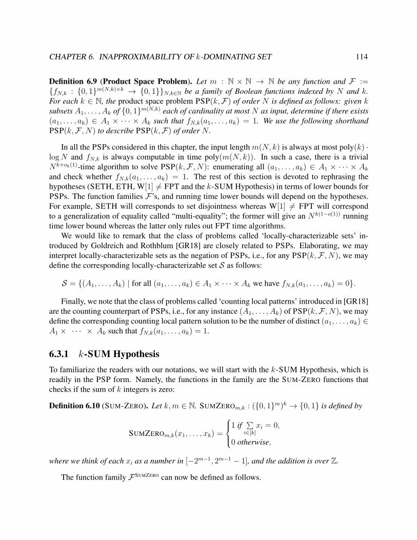
CHAPTER 6. INAPPROXIMABILITY OF k-DOMINATING SET 114
Definition 6.9 (Product Space Problem). Let m : N × N → N be any function and F :=fN,k : 0, 1m(N,k)×k → 0, 1N,k∈N be a family of Boolean functions indexed by N and k.For each k ∈ N, the product space problem PSP(k,F) of order N is defined as follows: given ksubsets A1, . . . , Ak of 0, 1m(N,k) each of cardinality at most N as input, determine if there exists(a1, . . . , ak) ∈ A1 × · · · × Ak such that fN,k(a1, . . . , ak) = 1. We use the following shorthandPSP(k,F , N) to describe PSP(k,F) of order N .
In all the PSPs considered in this chapter, the input length m(N, k) is always at most poly(k) ·logN and fN,k is always computable in time poly(m(N, k)). In such a case, there is a trivialNk+ok(1)-time algorithm to solve PSP(k,F , N): enumerating all (a1, . . . , ak) ∈ A1 × · · · × Akand check whether fN,k(a1, . . . , ak) = 1. The rest of this section is devoted to rephrasing thehypotheses (SETH, ETH, W[1] 6= FPT and the k-SUM Hypothesis) in terms of lower bounds forPSPs. The function families F’s, and running time lower bounds will depend on the hypotheses.For example, SETH will corresponds to set disjointness whereas W[1] 6= FPT will correspondto a generalization of equality called “multi-equality”; the former will give an Nk(1−o(1)) runningtime lower bound whereas the latter only rules out FPT time algorithms.
We would like to remark that the class of problems called ‘locally-characterizable sets’ in-troduced by Goldreich and Rothblum [GR18] are closely related to PSPs. Elaborating, we mayinterpret locally-characterizable sets as the negation of PSPs, i.e., for any PSP(k,F , N), we maydefine the corresponding locally-characterizable set S as follows:
S = (A1, . . . , Ak) | for all (a1, . . . , ak) ∈ A1 × · · · × Ak we have fN,k(a1, . . . , ak) = 0.
Finally, we note that the class of problems called ‘counting local patterns’ introduced in [GR18]are the counting counterpart of PSPs, i.e., for any instance (A1, . . . , Ak) of PSP(k,F , N), we maydefine the corresponding counting local pattern solution to be the number of distinct (a1, . . . , ak) ∈A1 × · · · × Ak such that fN,k(a1, . . . , ak) = 1.
6.3.1 k-SUM HypothesisTo familiarize the readers with our notations, we will start with the k-SUM Hypothesis, which isreadily in the PSP form. Namely, the functions in the family are the SUM-ZERO functions thatchecks if the sum of k integers is zero:
Definition 6.10 (SUM-ZERO). Let k,m ∈ N. SUMZEROm,k : (0, 1m)k → 0, 1 is defined by
SUMZEROm,k(x1, . . . , xk) =
1 if
∑i∈[k]
xi = 0,
0 otherwise,
where we think of each xi as a number in [−2m−1, 2m−1 − 1], and the addition is over Z.
The function family F SUMZERO can now be defined as follows.
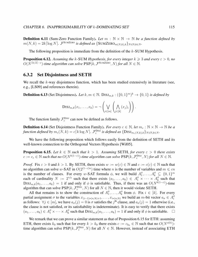
CHAPTER 6. INAPPROXIMABILITY OF k-DOMINATING SET 115
Definition 6.11 (Sum-Zero Function Family). Let m : N × N → N be a function defined bym(N, k) = 2kdlogNe. F SUMZERO is defined as SUMZEROm(N,k),kN∈N,k∈N .
The following proposition is immediate from the definition of the k-SUM Hypothesis.
Proposition 6.12. Assuming the k-SUM Hypothesis, for every integer k > 3 and every ε > 0, noO(N dk/2e−ε)-time algorithm can solve PSP(k,F SUMZERO, N) for all N ∈ N.
6.3.2 Set Disjointness and SETHWe recall the k-way disjointness function, which has been studied extensively in literature (see,e.g., [LS09] and references therein).
Definition 6.13 (Set Disjointness). Let k,m ∈ N. DISJm,k : (0, 1m)k → 0, 1 is defined by
DISJm,k(x1, . . . , xk) = ¬ ∨i∈[m]
∧j∈[k]
(xj)i
.The function family FDISJ
c can now be defined as follows.
Definition 6.14 (Set Disjointness Function Family). For every c ∈ N, let mc : N × N → N be afunction defined by mc(N, k) = cdk logNe. FDISJ
c is defined as DISJmc(N,k),kN∈N,k∈N .
We have the following proposition which follows easily from the definition of SETH and itswell-known connection to the Orthogonal Vectors Hypothesis [Wil05].
Proposition 6.15. Let k ∈ N such that k > 1. Assuming SETH, for every ε > 0 there existsc := cε ∈ N such that no O(Nk(1−ε))-time algorithm can solve PSP(k,FDISJ
c , N) for all N ∈ N.
Proof. Fix ε > 0 and k > 1. By SETH, there exists w := w(ε) ∈ N and c := c(ε) ∈ N such thatno algorithm can solve w-SAT in O(2(1−ε)n) time where n is the number of variables and m 6 cnis the number of clauses. For every w-SAT formula φ, we will build Aφ1 , . . . , A
φk ⊆ 0, 1m
each of cardinality N := 2n/k such that there exists (a1, . . . , ak) ∈ Aφ1 × · · · × Aφk such thatDISJm,k(a1, . . . , ak) = 1 if and only if φ is satisfiable. Thus, if there was an O(Nk(1−ε))-timealgorithm that can solve PSP(k,FDISJ
c , N) for all N ∈ N, then it would violate SETH.All that remains is to show the construction of Aφ1 , . . . , A
φk from φ. Fix i ∈ [k]. For every
partial assignment σ to the variables x(i−1)∗(n/k)+1, . . . , xi∗(n/k) we build an m-bit vector aσ ∈ Aφias follows: ∀j ∈ [m], we have aσ(j) = 0 is σ satisfies the j th clause, and aσ(j) = 1 otherwise (i.e.,the clause is not satisfied, or its satisfiability is indeterminate). It is easy to verify that there exists(a1, . . . , ak) ∈ Aφ1 × · · · ×Aφk such that DISJm,k(a1, . . . , ak) = 1 if and only if φ is satisfiable.
We remark that we can prove a similar statement as that of Proposition 6.15 for ETH: assumingETH, there exists k0 such that for every k > k0 there exists c := ck0 ∈ N such that no O(N o(k))-time algorithm can solve PSP(k,FDISJ
c , N) for all N ∈ N. However, instead of associating ETH
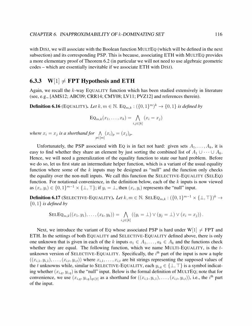
CHAPTER 6. INAPPROXIMABILITY OF k-DOMINATING SET 116
with DISJ, we will associate with the Boolean function MULTEQ (which will be defined in the nextsubsection) and its corresponding PSP. This is because, associating ETH with MULTEQ providesa more elementary proof of Theorem 6.2 (in particular we will not need to use algebraic geometriccodes – which are essentially inevitable if we associate ETH with DISJ).
6.3.3 W[1] 6= FPT Hypothesis and ETHAgain, we recall the k-way EQUALITY function which has been studied extensively in literature(see, e.g., [AMS12; ABC09; CRR14; CMY08; LV11; PVZ12] and references therein).
Definition 6.16 (EQUALITY). Let k,m ∈ N. EQm,k : (0, 1m)k → 0, 1 is defined by
EQm,k(x1, . . . , xk) =∧
i,j∈[k](xi = xj)
where xi = xj is a shorthand for∧
p∈[m](xi)p = (xj)p.
Unfortunately, the PSP associated with EQ is in fact not hard: given sets A1, . . . , Ak, it iseasy to find whether they share an element by just sorting the combined list of A1 ∪ · · · ∪ Ak.Hence, we will need a generalization of the equality function to state our hard problem. Beforewe do so, let us first state an intermediate helper function, which is a variant of the usual equalityfunction where some of the k inputs may be designed as “null” and the function only checksthe equality over the non-null inputs. We call this function the SELECTIVE-EQUALITY (SELEQ)function. For notational convenience, in the definition below, each of the k inputs is now viewedas (xi, yi) ∈ 0, 1m−1 × ⊥,>; if yi = ⊥, then (xi, yi) represents the “null” input.
Definition 6.17 (SELECTIVE-EQUALITY). Let k,m ∈ N. SELEQm,k : (0, 1m−1 × ⊥,>)k →0, 1 is defined by
SELEQm,k((x1, y1), . . . , (xk, yk)) =∧
i,j∈[k]((yi = ⊥) ∨ (yj = ⊥) ∨ (xi = xj)) .
Next, we introduce the variant of EQ whose associated PSP is hard under W[1] 6= FPT andETH. In the settings of both EQUALITY and SELECTIVE-EQUALITY defined above, there is onlyone unknown that is given in each of the k inputs a1 ∈ A1, . . . , ak ∈ Ak and the functions checkwhether they are equal. The following function, which we name MULTI-EQUALITY, is the t-unknown version of SELECTIVE-EQUALITY. Specifically, the ith part of the input is now a tuple((xi,1, yi,1), . . . , (xi,t, yi,t)) where xi,1, . . . , xi,t are bit strings representing the supposed values ofthe t unknowns while, similar to SELECTIVE-EQUALITY, each yi,q ∈ ⊥,> is a symbol indicat-ing whether (xi,q, yi,q) is the “null” input. Below is the formal definition of MULTEQ; note that forconvenience, we use (xi,q, yi,q)q∈[t] as a shorthand for ((xi,1, yi,1), . . . , (xi,t, yi,t)), i.e., the ith partof the input.
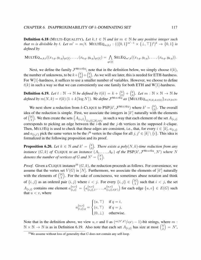
CHAPTER 6. INAPPROXIMABILITY OF k-DOMINATING SET 117
Definition 6.18 (MULTI-EQUALITY). Let k, t ∈ N and let m ∈ N be any positive integer suchthat m is divisible by t. Let m′ = m/t. MULTEQm,k,t : ((0, 1m′−1 × ⊥,>)t)k → 0, 1 isdefined by
MULTEQm,k,t((x1,q, y1,q)q∈[t], . . . , (xk,q, yk,q)q∈[t]) =∧q∈[t]
SELEQm′,k((x1,q, y1,q), . . . , (xk,q, yk,q)).
Next, we define the family FMULTEQ; note that in the definition below, we simply choose t(k),the number of unknowns, to be k+
(k2
)+(k3
). As we will see later, this is needed for ETH-hardness.
For W[1]-hardness, it suffices to use a smaller number of variables. However, we choose to definet(k) in such a way so that we can conveniently use one family for both ETH and W[1]-hardness.
Definition 6.19. Let t : N → N be defined by t(k) = k +(k2
)+(k3
). Let m : N × N → N be
defined by m(N, k) = t(k) (1 + kdlogNe). We define FMULTEQ as MULTEQm(N,k),k,t(k)N∈N,k∈N.
We next show a reduction from k-CLIQUE to PSP(k′,FMULTEQ) where k′ =(k2
). The overall
idea of the reduction is simple. First, we associate the integers in [k′] naturally with the elementsof(
[k]2
). We then create the sets
(Ai,j
)i,j⊆[k],i 6=j
in such a way that each element of the set Ai,jcorresponds to picking an edge between the i-th and the j-th vertices in the supposed k-clique.Then, MULTEQ is used to check that these edges are consistent, i.e., that, for every i ∈ [k], ai,jand ai,j′ pick the same vertex to be the ith vertex in the clique for all j, j′ ∈ [k] \ i. This idea isformalized in the following proposition and its proof.
Proposition 6.20. Let k ∈ N and k′ =(k2
). There exists a poly(N, k)-time reduction from any
instance (G, k) of CLIQUE to an instance (A1, . . . , Ak′) of the PSP(k′,FMULTEQ, N ′) where Ndenotes the number of vertices of G and N ′ =
(N2
).
Proof. Given a CLIQUE instance10 (G, k), the reduction proceeds as follows. For convenience, weassume that the vertex set V (G) is [N ]. Furthermore, we associate the elements of [k′] naturallywith the elements of
([k]2
). For the sake of conciseness, we sometimes abuse notation and think
of i, j as an ordered pair (i, j) where i < j. For every i, j ∈(
[k]2
)such that i < j, the set
Ai,j contains one element au,vi,j =(au,vi,j,1, . . . , a
u,vi,j,t(k′)
)for each edge u, v ∈ E(G) such
that u < v, where
au,vi,j,q =
(u,>) if q = i,
(v,>) if q = j,
(0,⊥) otherwise.
Note that in the definition above, we view u, v and 0 as (m(N ′,k′)/t(k′)− 1)-bit strings, where m :N × N → N is as in Definition 6.19. Also note that each set Ai,j has size at most
(N2
)= N ′,
10We assume without loss of generality that G does not contain any self-loop.
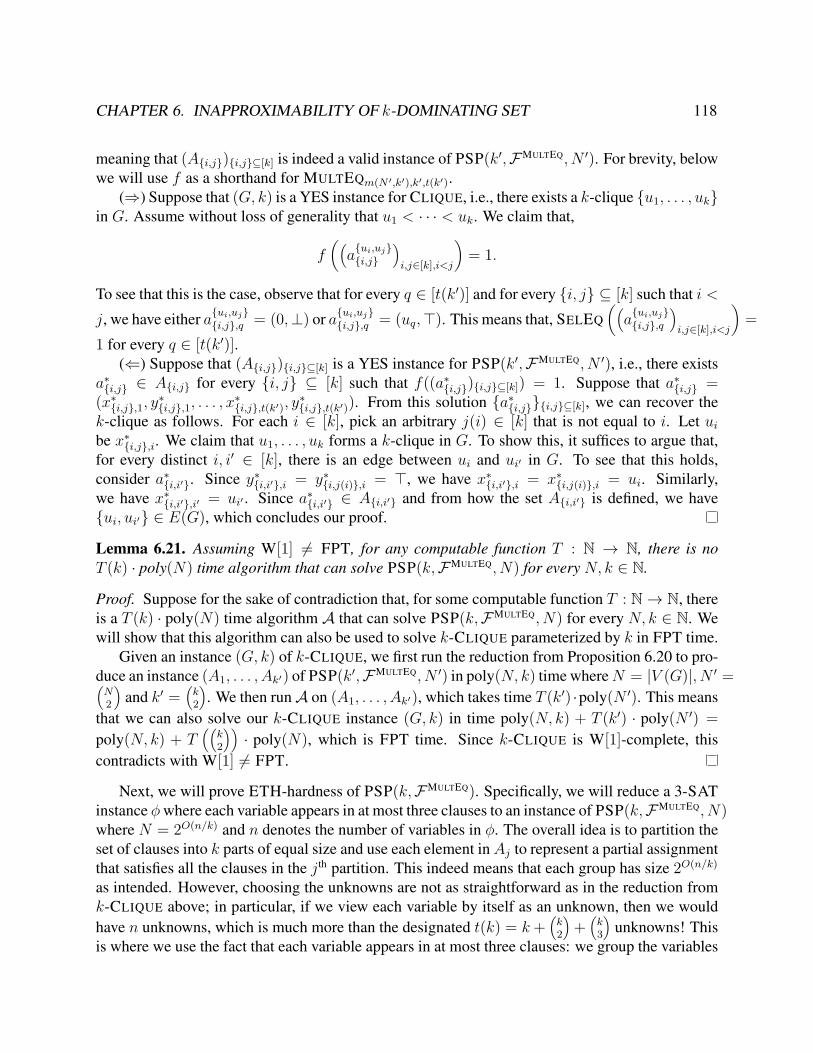
CHAPTER 6. INAPPROXIMABILITY OF k-DOMINATING SET 118
meaning that (Ai,j)i,j⊆[k] is indeed a valid instance of PSP(k′,FMULTEQ, N ′). For brevity, belowwe will use f as a shorthand for MULTEQm(N ′,k′),k′,t(k′).
(⇒) Suppose that (G, k) is a YES instance for CLIQUE, i.e., there exists a k-clique u1, . . . , ukin G. Assume without loss of generality that u1 < · · · < uk. We claim that,
f((aui,uji,j
)i,j∈[k],i<j
)= 1.
To see that this is the case, observe that for every q ∈ [t(k′)] and for every i, j ⊆ [k] such that i <
j, we have either aui,uji,j,q = (0,⊥) or aui,uji,j,q = (uq,>). This means that, SELEQ
((aui,uji,j,q
)i,j∈[k],i<j
)=
1 for every q ∈ [t(k′)].(⇐) Suppose that (Ai,j)i,j⊆[k] is a YES instance for PSP(k′,FMULTEQ, N ′), i.e., there exists
a∗i,j ∈ Ai,j for every i, j ⊆ [k] such that f((a∗i,j)i,j⊆[k]) = 1. Suppose that a∗i,j =(x∗i,j,1, y∗i,j,1, . . . , x∗i,j,t(k′), y∗i,j,t(k′)). From this solution a∗i,ji,j⊆[k], we can recover thek-clique as follows. For each i ∈ [k], pick an arbitrary j(i) ∈ [k] that is not equal to i. Let uibe x∗i,j,i. We claim that u1, . . . , uk forms a k-clique in G. To show this, it suffices to argue that,for every distinct i, i′ ∈ [k], there is an edge between ui and ui′ in G. To see that this holds,consider a∗i,i′. Since y∗i,i′,i = y∗i,j(i),i = >, we have x∗i,i′,i = x∗i,j(i),i = ui. Similarly,we have x∗i,i′,i′ = ui′ . Since a∗i,i′ ∈ Ai,i′ and from how the set Ai,i′ is defined, we haveui, ui′ ∈ E(G), which concludes our proof.
Lemma 6.21. Assuming W[1] 6= FPT, for any computable function T : N → N, there is noT (k) · poly(N) time algorithm that can solve PSP(k,FMULTEQ, N) for every N, k ∈ N.
Proof. Suppose for the sake of contradiction that, for some computable function T : N→ N, thereis a T (k) · poly(N) time algorithm A that can solve PSP(k,FMULTEQ, N) for every N, k ∈ N. Wewill show that this algorithm can also be used to solve k-CLIQUE parameterized by k in FPT time.
Given an instance (G, k) of k-CLIQUE, we first run the reduction from Proposition 6.20 to pro-duce an instance (A1, . . . , Ak′) of PSP(k′,FMULTEQ, N ′) in poly(N, k) time whereN = |V (G)|, N ′ =(N2
)and k′ =
(k2
). We then runA on (A1, . . . , Ak′), which takes time T (k′) ·poly(N ′). This means
that we can also solve our k-CLIQUE instance (G, k) in time poly(N, k) + T (k′) · poly(N ′) =poly(N, k) + T
((k2
))· poly(N), which is FPT time. Since k-CLIQUE is W[1]-complete, this
contradicts with W[1] 6= FPT.
Next, we will prove ETH-hardness of PSP(k,FMULTEQ). Specifically, we will reduce a 3-SATinstance φwhere each variable appears in at most three clauses to an instance of PSP(k,FMULTEQ, N)where N = 2O(n/k) and n denotes the number of variables in φ. The overall idea is to partition theset of clauses into k parts of equal size and use each element inAj to represent a partial assignmentthat satisfies all the clauses in the j th partition. This indeed means that each group has size 2O(n/k)
as intended. However, choosing the unknowns are not as straightforward as in the reduction fromk-CLIQUE above; in particular, if we view each variable by itself as an unknown, then we wouldhave n unknowns, which is much more than the designated t(k) = k +
(k2
)+(k3
)unknowns! This
is where we use the fact that each variable appears in at most three clauses: we group the variables
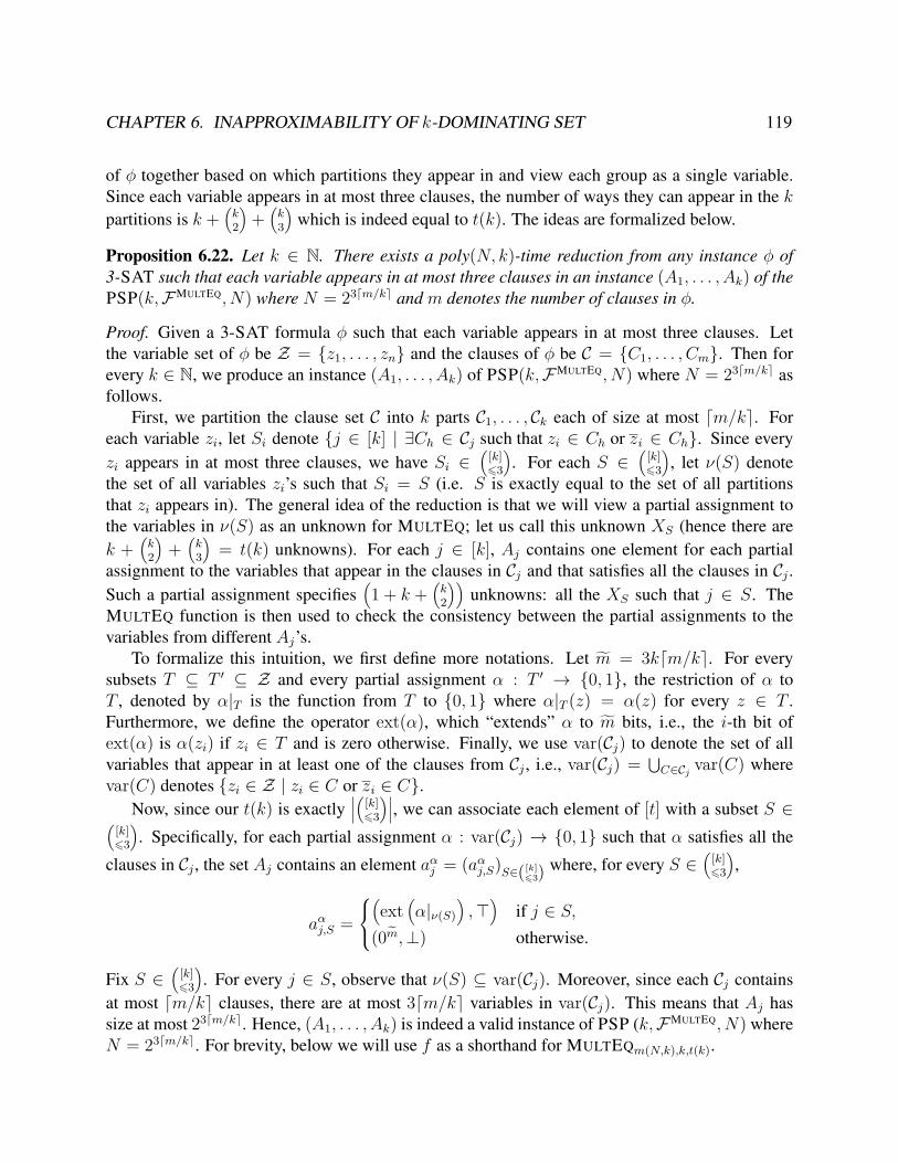
CHAPTER 6. INAPPROXIMABILITY OF k-DOMINATING SET 119
of φ together based on which partitions they appear in and view each group as a single variable.Since each variable appears in at most three clauses, the number of ways they can appear in the kpartitions is k +
(k2
)+(k3
)which is indeed equal to t(k). The ideas are formalized below.
Proposition 6.22. Let k ∈ N. There exists a poly(N, k)-time reduction from any instance φ of3-SAT such that each variable appears in at most three clauses in an instance (A1, . . . , Ak) of thePSP(k,FMULTEQ, N) where N = 23dm/ke and m denotes the number of clauses in φ.
Proof. Given a 3-SAT formula φ such that each variable appears in at most three clauses. Letthe variable set of φ be Z = z1, . . . , zn and the clauses of φ be C = C1, . . . , Cm. Then forevery k ∈ N, we produce an instance (A1, . . . , Ak) of PSP(k,FMULTEQ, N) where N = 23dm/ke asfollows.
First, we partition the clause set C into k parts C1, . . . , Ck each of size at most dm/ke. Foreach variable zi, let Si denote j ∈ [k] | ∃Ch ∈ Cj such that zi ∈ Ch or zi ∈ Ch. Since everyzi appears in at most three clauses, we have Si ∈
([k]63
). For each S ∈
([k]63
), let ν(S) denote
the set of all variables zi’s such that Si = S (i.e. S is exactly equal to the set of all partitionsthat zi appears in). The general idea of the reduction is that we will view a partial assignment tothe variables in ν(S) as an unknown for MULTEQ; let us call this unknown XS (hence there arek +
(k2
)+(k3
)= t(k) unknowns). For each j ∈ [k], Aj contains one element for each partial
assignment to the variables that appear in the clauses in Cj and that satisfies all the clauses in Cj .Such a partial assignment specifies
(1 + k +
(k2
))unknowns: all the XS such that j ∈ S. The
MULTEQ function is then used to check the consistency between the partial assignments to thevariables from different Aj’s.
To formalize this intuition, we first define more notations. Let m = 3kdm/ke. For everysubsets T ⊆ T ′ ⊆ Z and every partial assignment α : T ′ → 0, 1, the restriction of α toT , denoted by α|T is the function from T to 0, 1 where α|T (z) = α(z) for every z ∈ T .Furthermore, we define the operator ext(α), which “extends” α to m bits, i.e., the i-th bit ofext(α) is α(zi) if zi ∈ T and is zero otherwise. Finally, we use var(Cj) to denote the set of allvariables that appear in at least one of the clauses from Cj , i.e., var(Cj) = ⋃
C∈Cj var(C) wherevar(C) denotes zi ∈ Z | zi ∈ C or zi ∈ C.
Now, since our t(k) is exactly∣∣∣([k]
63
)∣∣∣, we can associate each element of [t] with a subset S ∈([k]63
). Specifically, for each partial assignment α : var(Cj) → 0, 1 such that α satisfies all the
clauses in Cj , the set Aj contains an element aαj = (aαj,S)S∈([k]
63) where, for every S ∈(
[k]63
),
aαj,S =
(ext
(α|ν(S)
),>)
if j ∈ S,(0m,⊥) otherwise.
Fix S ∈(
[k]63
). For every j ∈ S, observe that ν(S) ⊆ var(Cj). Moreover, since each Cj contains
at most dm/ke clauses, there are at most 3dm/ke variables in var(Cj). This means that Aj hassize at most 23dm/ke. Hence, (A1, . . . , Ak) is indeed a valid instance of PSP (k,FMULTEQ, N) whereN = 23dm/ke. For brevity, below we will use f as a shorthand for MULTEQm(N,k),k,t(k).
CHAPTER 6. INAPPROXIMABILITY OF k-DOMINATING SET 120
(⇒) Suppose that φ is satisfiable. Let α : C → 0, 1 be an assignment that satisfies all the
clauses. Let a∗j = aα|var(Cj)j ∈ Aj for every j ∈ [k]. Observe that, for every S ∈
([k]63
)and every
j ∈ [k], we either have a∗j,S = (0m,⊥) or a∗j,S = (ext(α|ν(S)),>). This indeed implies thatf(a∗1, . . . , a∗k) = 1.
(⇐) Suppose that there exists (aα11 , . . . , a
αkk ) ∈ A1 × · · · × Ak such that f(aα1
1 , . . . , aαkk ) = 1.
We construct an assignment α : Z → 0, 1 as follows. For each i ∈ [n], pick an arbitraryj(i) ∈ [k] such that zi ∈ var(Cj(i)) and let α(zi) = αj(i)(zi). We claim that α satisfies every clause.To see this, consider any clause C ∈ C. Suppose that C is in the partition Cj . It is easy to checkthat f(aα1
1 , . . . , aαkk ) = 1 implies that α|var(C) = αj|var(C). Since αj is a partial assignment that
satisfies C, α must also satisfy C. In other words, α satisfies all clauses of φ.
Lemma 6.23. Assuming ETH, for any computable function T : N → N, there is no T (k) · N o(k)
time algorithm that can solve PSP(k,FMULTEQ, N) for every N, k ∈ N.
Proof. Let δ > 0 be the constant in the running time lower bound in ETH. Suppose for the sakeof contradiction that ETH holds but, for some function T , there is a T (k) · N o(k) time algorithmA that can solve PSP(k,FMULTEQ, N) for every N, k ∈ N. Thus, there exists a sufficiently largek such that the running time of A for solving PSP(k,FMULTEQ, N) is at most O(N δk/10) for everyN ∈ N.
Given a 3-CNF formula φ such that each variable appears in at most three clauses. Let n,mdenote the number of variables and the number of clauses of φ, respectively. We first run thereduction from Proposition 6.22 on φ with this value of k. This produces an instance (A1, . . . , Ak)of PSP (k,FMULTEQ, N) where N = 23dm/ke. Since each variable appears in at most three clauses,we have m 6 3n, meaning that N = O(29n/k). By running A on this instance, we can decidewhether φ is satisfiable in time O(N δk/10) = O(20.9δn), contradicting ETH.
6.4 Communication Protocols and Reduction to MAXCOV
In this section, we first introduce a communication model for multiparty communication known inliterature as the Simultaneous Message Passing model. Then, we introduce a notion of “efficient”communication protocols, and connect the existence of such protocols to a reduction from PSP toa gap version of MAXCOV.
6.4.1 Efficient Protocols in Simultaneous Message Passing ModelThe two-player Simultaneous Message Passing (SMP) model was introduced by Yao [Yao79] andhas been extensively studied in literature [KN97]. In the multiparty setting, the SMP model isconsidered popularly with the number-on-forehead model, where each player can see the input ofall the other players but not his own [CFL83; Bab+03]. In this chapter, we consider the multipartySMP model where the inputs are given as in the number-in-hand model (like in [FOZ16; WW15]).
CHAPTER 6. INAPPROXIMABILITY OF k-DOMINATING SET 121
Simultaneous Message Passing Model. Let f : 0, 1m×k → 0, 1. In the k-player simulta-neous message passing communication model, we have k players each with an input xi ∈ 0, 1mand a referee who is given an advice µ ∈ 0, 1∗ (at the same time when the players are given theinput). The communication task is for the referee to determine if f(x1, . . . , xk) = 1. The playersare allowed to only send messages to the referee. In the randomized setting, we allow the playersand the referee to jointly toss some random coins before sending messages, i.e., we allow publicrandomness.
Next, we introduce the notion of efficient protocols, which are in a nutshell one-round random-ized protocols where the players and the referee are in a computationally bounded setting.
Efficient Protocols. Let π be a communication protocol for a problem in the SMP model. Wesay that π is a (w, r, `, s)-efficient protocol if the following holds:
• The referee receives w bits of advice.
• The protocol is one-round with public randomness, i.e., the following actions happen se-quentially:
1. The players receive their inputs and the referee receives his advice.2. The players and the referee jointly toss r random coins.3. Each player on seeing the randomness (i.e. results of r coin tosses) deterministically
sends an `-bit message to the referee.4. Based on the advice, the randomness, and the total ` · k bits sent from the players, the
referee outputs accept or reject.
• The protocol has completeness 1 and soundness s, i.e.,
– If f(x1, . . . , xk) = 1, then there exists an advice on which the referee always accepts.– If f(x1, . . . , xk) = 0, then, on any advice, the referee accepts with probability at mosts.
• The players and the referee are computationally bounded, i.e., all of them perform all theircomputations in poly(m)-time.
The following proposition follows immediately from the definition of an efficient protocol andwill be very useful in later sections for gap amplification.
Proposition 6.24. Let z ∈ N and π be a communication protocol for a problem in the SMP model.Suppose π is a (w, r, `, s)-efficient protocol. Then there exists a (w, z · r, z · `, sz)-efficient protocolfor the same problem.
Proof. The proof follows by a simple repetition argument. More precisely, we repeat steps 2-4in the protocol z times, each time using fresh randomness, but note that the z steps of drawingrandom coins can be clubbed into one step, and the decision by the referee can be reserved tillthe end of the entire protocol, wherein he accepts if and only if he would accept in each of theindividual repetitions.
CHAPTER 6. INAPPROXIMABILITY OF k-DOMINATING SET 122
6.4.2 Lower Bounds on Gap-MAXCOV
The following theorem is the main conceptual contribution of the chapter: we show below that theexistence of efficient protocols can translate (exact) hardness of PSPs to hardness of approximatingMAXCOV.
Theorem 6.25. Let m : N × N → N be any function. Let F := fN,k : 0, 1m(N,k)×k →0, 1N,k∈N be a family of Boolean functions indexed by N, k. Suppose there exists a (w, r, `, s)-efficient protocol11 for fN,k in the k-player SMP model for every N, k ∈ N. Then, there is a re-duction from any instance (A1, . . . , Ak) of PSP(k,F , N) to 2w label cover instances Lµµ∈0,1wsuch that
• The running time of the reduction is 2w+r+`kpoly(m(N, k)).
• Each Lµ = (Uµ, V µ,ΣµU ,Σ
µV , Πµ
e) has the following parameters:
– Lµ has k right super nodes, i.e., |V µ| = k,
– Lµ has 2r left super nodes, i.e., |Uµ| = 2r,– Lµ’s right alphabet size is at most N right nodes, i.e., |Σµ
V | 6 N ,
– Lµ’s left alphabet size is at most 2`k, i.e., |ΣµU | 6 2`k.
• If (A1, . . . , Ak) is a YES instance of PSP(k,F , N), then MAXCOV(Lµ) = 2r for someµ ∈ 0, 1w.
• If (A1, . . . , Ak) is a NO instance of PSP(k,F , N), then MAXCOV(Lµ) 6 s · 2r for everyµ ∈ 0, 1w.
Proof. Given a (w, r, `, s)-efficient protocol π of fN,k and an instance (A1, . . . , Ak) of PSP(k,F , N),we will generate 2w instances of MAXCOV. Specifically, for each µ ∈ 0, 1w, we construct aninstance Lµ = (Uµ, V µ,Σµ
U ,ΣµV , Πµ
e) of MAXCOV as follows.
• Let V µ = [k].
• Let ΣµV be of size N , and, for each j ∈ [h], we associate each xj ∈ Aj with a label in Σµ
V .
• Let Uµ = 0, 1r.
• Let ΣµU be of size 2`k. For each left super-node γ ∈ 0, 1r, we associate each accepting
messages from the k players (i.e. (m1, . . . ,mk) ∈ (0, 1`)k where in the protocol π thereferee, on an advice µ and a random string γ, accepts if the messages he received from thek players are m1, . . . ,mk) with a label in Σµ
U .
• For each e = (j, γ), we add an (xj, (m1, . . . ,mk)) to Πe iff mj is equal to the message thatj sends on an input xj and a random string γ in the protocol π.
11w, r, ` and s can depend on N and k.
CHAPTER 6. INAPPROXIMABILITY OF k-DOMINATING SET 123
Note here that, since |Aj|’s may not be equal, some label in ΣµV might not be associated with any
element in Aj for some left super-node j. In this case, we might ignore such a label for the super-node j since it never appears in the constraints. Similar statement holds for the right super-nodes.From this viewpoint, there is a bijection between “valid” right labelings of Lµ and elements ofA1 × · · · × Ak, where “valid” means that these labels are not used.
Now consider a right labeling σV µ of Lµ and the corresponding (x1, . . . , xk) ∈ A1 × · · · ×Ak.For each random string γ ∈ 0, 1r, observe that the referee accepts on an input (x1, . . . , xk), anadvice µ, and a random string γ if and only if there is a label (m1, . . . ,mk) of the left super-nodeγ that is consistent with all of x1, . . . , xk. Therefore, the acceptance probability of the protocolon advice µ is the same as the fraction of left super-nodes covered by σV µ . The completeness andsoundness then easily follows:
Completeness. If there exists (x1, . . . , xk) ∈ A1 × · · · × Ak such that fN,k(x1, . . . , xk) = 1,then there is an advice µ ∈ 0, 1w on which the referee always accepts for this input (x1, . . . , xk),meaning that the corresponding labeling covers every left super-node of Lµ, i.e., MAXCOV(Lµ) =2r.
Soundness. If fN,k(x1, . . . , xk) = 0 for every (x1, . . . , xk) ∈ A1 × · · · × Ak, then, for anyadvice µ ∈ 0, 1w, the referee accepts with probability at most s on every input (x1, . . . , xk) ∈A1 × · · · × Ak. This means that, for any µ ∈ 0, 1w, no labeling covers more than s fraction ofleft the super-nodes. In other words, MAXCOV(Lµ) 6 s · 2r for all µ ∈ 0, 1w.
For the rest of this subsection, we will use the following shorthand. LetL = (U, V,ΣU ,ΣV , Πe)be a label cover instance, and we use the shorthand L(N, k, r, `) to say that the label cover instancehas the following parameters:
• L has k right super nodes, i.e., |V | = k,
• L has 2r left super nodes, i.e., |U | = 2r,
• L has right alphabet size of at most N , i.e., |ΣV | 6 N ,
• L has left alphabet size of at most 2`k, i.e., |ΣU | 6 2`k.
The rest of this section is devoted to combining Theorem 6.25 with the results in Section 6.3to obtain conditional hardness for the gap-MAXCOV problem, assuming that we have efficientprotocols with certain parameters. These protocols will be devised in the three subsequent sections.
Understanding the Parameters. Before we state the exact dependency of parameters, let usfirst discuss some intuition behind it. First of all, if we start with an instance of PSP(k,F , N),Theorem 6.25 will produce 2w instances of L(N, k, r, `). Roughly speaking, since we want thelower bounds from PSP to translate to MAXCOV, we would like the number of instances to beN o(1), meaning that we want w = o(logN). Recall that in all function families we considerm = Θk(logN). Hence, this requirement is the same as w = ok(m). Moreover, we would like theinstance size of L(N, k, r, `) to also be Ok(N), meaning that |U ||ΣU | 6 2r+`k has to be Ok(N).Thus, it suffices to have a protocol where r + `k = ok(m).
CHAPTER 6. INAPPROXIMABILITY OF k-DOMINATING SET 124
If we additionally want the hardness to translate also to k-DOMSET, the parameter dependen-cies become more subtle. Specifically, applying Theorem 2.27 to the MAXCOV instances results ina blow-up of |U ||V ||ΣU | 6 2r · k2`k = 2r+(log k)·2`k . We also want this to be at most N o(1), meaningthat we need r+ (log k) · 2`k = o(logN) = ok(m). In other words, it suffices for us to require that`k < (logm)/β for some constant β > 1. The exact parameter dependencies are formalized below.
SETH
Corollary 6.26. For any c ∈ N, let FDISJc be the family of Boolean functions as defined in Defini-
tion 6.14. For every δ > 0, suppose there exists a (w, r, `, s)-efficient protocol for DISJm,k in thek-player SMP model for every k ∈ N and every m ∈ N, such that w 6 δm and r + `k = ok(m).Then, assuming SETH, for every ε > 0 and integer k > 1, no O(Nk(1−ε))-time algorithm candistinguish between MAXCOV(L) = 2r and MAXCOV(L) 6 s · 2r for any label cover instanceL(N, k, r, `) for all N ∈ N. Moreover, if ` < (logm)/β·k for some constant β > 1, then assumingSETH, for every ε > 0 and integer k > 1, no O(Nk(1−ε))-time algorithm can distinguish between
DOMSET(G) = k and DOMSET(G) >(
1s
) 1k · k for any graph G with at most Ok(N) vertices, for
all N ∈ N.
Proof. The proof of the first part of the theorem statement is by contradiction. Suppose there isan O(Nk(1−ε))-time algorithm A for some fixed constant ε > 0 and integer k > 1 which candistinguish between MAXCOV(L) = 2r and MAXCOV(L) 6 s · 2r for any label cover instanceL(N, k, r, `) for all N ∈ N. From Proposition 6.15, we have that there exists cε ∈ N such thatno O(Nk(1−ε/2))-time algorithm can solve PSP(k,FDISJ
cε , N) for all N ∈ N. Fix δ = ε/3cε. Next,by considering Theorem 6.25 for the case of (w, r, `, s)-efficient protocols, we have that thereare 2w label cover instances Lµµ∈0,1w which can be constructed in 2δm(1+ok(1)) time. Notethat 2δm(1+ok(1)) = N kε/3(1+ok(1)) by our choice of δ. Thus, we can run A on each Lµ and solvePSP(k,FDISJ
c , N) for all N, k ∈ N in time less than Nk(1−ε/2). This contradicts Proposition 6.15.To prove the second part of the theorem statement, we apply the reduction described in Theo-
rem 2.27 and note that 2r = N o(1) and k2`k = 2(log2 k)·(m(N,k))1/β = N o(1).
The proof of Theorem 6.3 follows by plugging in the parameters of the protocol described inCorollary 6.31 to the above corollary.
ETH
Corollary 6.27. Let FMULTEQ be the family of Boolean functions as defined in Definition 6.19.Suppose there exists a (w, r, `, s)-efficient protocol for MULTEQm,k,t in the k-player SMP modelfor every k, t,m ∈ N such that w + r + `k = ok(m). Then, assuming ETH, for any com-putable function T : N→ N, there is no T (k) ·N o(k) time algorithm that can distinguish betweenMAXCOV(L) = 2r and MAXCOV(L) 6 s · 2r for any label cover instance L(N, k, r, `) for allN, k ∈ N. Moreover, if ` < (logm)/β·k for some constant β > 1, then assuming ETH, for any com-putable function T : N→ N, there is no T (k) ·N o(k) time algorithm that can distinguish between
CHAPTER 6. INAPPROXIMABILITY OF k-DOMINATING SET 125
DOMSET(G) = k and DOMSET(G) >(
1s
) 1k · k for any graph G with at most Ok(N) vertices, for
all N, k ∈ N.
Proof. The proof of the first part of the theorem statement is by contradiction. Suppose there isan algorithm A running in time T (k) · N o(k) for some computable function T : N → N that candistinguish between MAXCOV(L) = 2r and MAXCOV(L) 6 s · 2r for any label cover instanceL(N, k, r, `) for all N, k ∈ N. From Lemma 6.23, we have that for any computable functionT : N → N, there is no T (k) · N o(k) time algorithm that can solve PSP(k,FMULTEQ, N) for everyN, k ∈ N. Next, by considering Theorem 6.25 for the case of (w, r, `, s)-efficient protocols, wehave that there are 2w label cover instances Lµµ∈0,1w which can be constructed in 2ok(m) time.Note that 2ok(m) = Ok(N o(1)) by the choice of m(N, k) in Definition 6.19. Thus, we can run Aon each Lµ and solve PSP(k,FMULTEQ, N) for all N, k ∈ N in time T (k) ·N o(k). This contradictsLemma 6.23.
To prove the second part of the theorem statement, we apply the reduction described in Theo-rem 2.27 and note that 2r = N o(1) and k2`k = 2(m(N,k))1/β ·log2 k = N o(1).
The proof of Theorem 6.2 follows by plugging in the parameters of the protocol described inCorollary 6.33 to the above corollary.
W[1] 6= FPT
Corollary 6.28. Let FMULTEQ be the family of Boolean functions as defined in Definition 6.19.Suppose there exists a (w, r, `, s)-efficient protocol for MULTEQm,k,t in the k-player SMP modelfor every k, t,m ∈ N such that w + r + `k < m/tk. Then, assuming W[1] 6= FPT, for anycomputable function T : N → N, there is no T (k) · poly(N)-time algorithm that can distinguishbetween MAXCOV(L) = 2r and MAXCOV(L) 6 s · 2r for any label cover instance L(N, k, r, `)for all N, k ∈ N. Moreover, if r < m/2tk and ` < (logm)/β·k for some constant β > 1, then assumingW[1] 6= FPT, for any computable function T : N→ N, there is no T (k) · poly(N)-time algorithm
that can distinguish between DOMSET(G) = k and DOMSET(G) >(
1s
) 1k · k for any graph G
with at most Ok(N) vertices, for all N, k ∈ N.
Proof. The proof of the first part of the theorem statement is by contradiction. Suppose there is analgorithm A running in time T (k) · poly(N) for some computable function T : N → N that candistinguish between MAXCOV(L) = 2r and MAXCOV(L) 6 s · 2r for any label cover instanceL(N, k, r, `) for all N, k ∈ N. From Lemma 6.21, we have that for any computable functionT : N→ N, there is no T (k)·poly(N) time algorithm that can solve PSP(k,FMULTEQ, N) for everyN, k ∈ N. Next, by considering Theorem 6.25 for the case of (w, r, `, s)-efficient protocols, wehave that there are 2w label cover instances Lµµ∈0,1w which can be constructed in 2m(N,k)/k·t(k) ·poly(m(N, k)) time. Note that 2m(N,k)/k·t(k) = O(N) and poly(m(N, k)) = N o(1) by the choice ofm(N, k) in Definition 6.19. Thus, we can run A on each Lµ and solve PSP(k,FMULTEQ, N) for allN, k ∈ N in time less than T (k) · poly(N). This contradicts Lemma 6.21.
CHAPTER 6. INAPPROXIMABILITY OF k-DOMINATING SET 126
To prove the second part of the theorem statement, we apply the reduction described in Theo-rem 2.27 and note that 2r = O(
√N) and k2`k = 2(m(N,k))1/β ·log2 k = N o(1).
The proof of Theorem 6.1 follows by plugging in the parameters of the protocol described inCorollary 6.33 to the above corollary.
k-SUM Hypothesis
Corollary 6.29. Let F SUMZERO be the family of Boolean functions as defined in Definition 6.11.Suppose there exists a (w, r, `, s)-efficient protocol for SUMZEROm,k in the k-player SMP modelfor every m, k ∈ N, such that w + r + `k = ok(m). Then assuming the k-SUM Hypothesis,for every integer k > 3 and every ε > 0, no O(N dk/2e−ε)-time algorithm can distinguish betweenMAXCOV(L) = 2r and MAXCOV(L) 6 s·2r for any label cover instanceL(N, k, r, `) for allN ∈N. Moreover, if ` < (logm)/β·k for some constant β > 1, then assuming the k-SUM Hypothesis,for every ε > 0 no O(N dk/2e−ε)-time algorithm can distinguish between DOMSET(G) = k and
DOMSET(G) >(
1s
) 1k · k for any graph G with at most Ok(N) vertices for all N ∈ N.
Proof. The proof of the first part of the theorem statement is by contradiction. Suppose there is analgorithm A running in time O(N dk/2e−ε) for some fixed constant ε > 0 and some integer k > 3that can distinguish between MAXCOV(L) = 2r and MAXCOV(L) 6 s · 2r for any label cover in-stance L(N, k, r, `) for all N ∈ N. From Proposition 6.12, we have that no O(N dk/2e−ε/2)-time al-gorithm can solve PSP(k,F SUMZERO, N) for all N ∈ N. Next, by considering Theorem 6.25 for thecase of (w, r, `, s)-efficient protocols, we have that there are 2w label cover instances Lµµ∈0,1wwhich can be constructed in 2ok(m) time. Note that 2ok(m) = Ok(N o(1)) by the choice of m(N, k)in Definition 6.11. Thus, we can run A on each Lµ and solve PSP(k,F SUMZERO, N) for all N ∈ Nin time O(N dk/2e−ε). This contradicts Proposition 6.12.
To prove the second part of the theorem statement, we apply the reduction described in Theo-rem 2.27 and note that 2r = N o(1) and k2`k = 2(m(N,k))1/β ·log2 k = N o(1).
The proof of Theorem 6.4 follows by plugging in the parameters of the protocol described inCorollary 6.39 to the above corollary.
6.5 An Efficient Protocol for Set DisjointnessSet Disjointness has been extensively studied primarily in the two-player setting (i.e., k = 2).In that setting, we know that the randomized communication complexity is Ω(m) [KS92; Raz92;Bar+04], where m is the input size of each player. Surprisingly, [AW09] showed that the MA-complexity of two-player set disjointness is O(
√m). Their protocol was indeed an (O(
√m), O(logm), O(
√m), 1/2)-
efficient protocol for the case when k = 2. Recently, [ARW17a] improved (in terms of themessage size) the protocol to be an (m/logm, O(logm), O((logm)3), 1/2)-efficient protocol for thecase when k = 2. Both these results can be extended naturally for all k > 1, to give an
CHAPTER 6. INAPPROXIMABILITY OF k-DOMINATING SET 127
(mk/logm, Ok(logm), Ok((logm)3), 1/2)-efficient protocol. However, this does not suffice for prov-ing Theorem 6.3 since we need a (w, r, `, s)-efficient protocol with w = o(m) and ` = o(logm).Fortunately, Rubinstein [Rub18] recently showed that the exact framework of the MA-protocolsas in [AW09; ARW17a] but with the use of algebraic geometric codes instead of Reed Mulleror Reed Solomon codes gives the desired parameters in the two-player case. Below we naturallyextend Rubinstein’s protocol to the k-player setting. This extension was suggested to us by Rubin-stein [Rub17a].
Theorem 6.30. There is a polynomial function ˆ : N × N → [1,∞) such that for every k ∈N and every α ∈ N, there is a protocol for k-player DISJm,k in the SMP model which is an(m/α, log2m,
ˆ(k, α), 1/2)-efficient protocol, where each player is given m bits as input, and thereferee is given at most m/α bits of advice.
Proof. Fix k,m, α ∈ N. Let q be the smallest prime greater than q(k) such that q > (2αr(k))2,where the functions r and q are as defined in Theorem 6.8. Let G = Fq2 . Let T = 2αr(k) log2 q.
We associate [m] with [T ] × [m/T ] and write the input xj ∈ 0, 1m as vectors x1j , . . . ,xTj
where xtj ∈ 0, 1m/T . For every j ∈ [k], Player j computes Am/T (xtj) for every t ∈ [T ]. Wedenote the block length of Am/T by d. From the systematicity guaranteed by Theorem 6.8 we havethat Am/T (xtj) |[m/T ]= xtj . Also, notice that for all t ∈ [T ], we have ∧
j∈[k]xtj = 0m/T if and only if∏
j∈[k] Am/T (xtj) = 0m/T .With the above observation in mind, we define the marginal sum Γ ∈ Gd as follows:
∀i ∈ [d], Γi =∑t∈[T ]
∏j∈[k]
Am/T (xtj)i.
Again, notice that for all t ∈ [T ], we have ∧j∈[k]
xtj = 0m/T if and only if Γi = 0 for all i ∈ [m/T ].This follows from the following:
• For all i ∈ [m/T ], we have Am/T (xtj)i ∈ 0, 1 and thus∏j∈[k]
Am/T (xtj)i ∈ 0, 1.
• The characteristic of G being greater than (2αr(k)) · √q > (2αr(k)) · log2 q = T .
More importantly, we remark that Γ is a codeword12 in Bm/T . This follows because Bm/T
is a degree k closure code of Am/T . To see this, in Definition 6.7, set t = k, r = k · T , andP [x1,1, . . . , xk,T ] = ∑
i∈[T ]∏j∈[k] xi,j .
The protocol
1. Merlin sends the referee Φ which is allegedly equal to the marginal sums codeword Γ definedabove.
12We would like to remark that we use the multiplicity of Algebraic Geometric codes to find a non-trivial advice.On a related note, Meir [Mei13] had previously shown that error correcting codes with the multiplicity property sufficeto show the IP theorem (i.e., the IP=PSPACE result).
CHAPTER 6. INAPPROXIMABILITY OF k-DOMINATING SET 128
2. All players jointly draw r ∈ [d] uniformly at random.
3. For every j ∈ 1, . . . , k, Player j sends to the referee Am/T (xtj)r, ∀t ∈ [T ].
4. The referee accepts if and only if both of the following hold:
∀i ∈ [m/T ], Φi = 0 (6.1)
Φr =∑t∈[T ]
∏j∈[k]
Am/T (xtj)r. (6.2)
Analysis
Advice Length. To send the advice, Merlin only needs to send a codeword in Bm/T to the verifier.This means that the advice length (in bits) is no more than log2 q
2 times the block length, whichis d 6 (m/T) r(k) = m/2α log2 q where the equality comes from our choice of T and the inequalityfrom Theorem 6.8.
Message Length. Each player sends T elements of G. Hence, the message length is T log2 q2 6
αr(k)(2 log2 q)2. Recall that q can be upper bounded by a polynomial in k and α. Hence, the mes-sage length is upper bounded entirely as a polynomial in k and α as desired.
Randomness. The number of coin tosses is log2(d) 6 log2 (mr(k)/T) = log2 (m/2α log2 q) <log2m.
Completeness. If the k sets are disjoint, Merlin can send the true Γ, and the verifier alwaysaccepts.
Soundness. If the k sets are not disjoint and Φ is actually Γ, then (6.1) is false and the verifieralways rejects. On the other hand, if Φ 6= Γ, then, since both are codewords of Bm/T , fromTheorem 6.8 their relative distance must be at least 1/2. As a result, with probability at least 1/2,Φr 6= Γr. Since the right hand side of (6.2) is simply Γr, the verifier will reject for such r. Hence,the rejection probability is at least 1/2.
The following corollary follows immediately by applying Proposition 6.24 with z = (log2 m)/2k·`(k,α)
to the above theorem.
Corollary 6.31. There is a polynomial function s : N × N → [1,∞) such that for every k ∈N and every α ∈ N there is a protocol for k-player DISJm,k in the SMP model which is an(m/α, O ((log2m)2) , (log2 m)/2k, (1/m)1/s(k,α)
)-efficient protocol, where each player is given m bits
as input, and the referee is given at most m/α bits of advice.
6.6 An Efficient Protocol for MULTI-EQUALITY
EQUALITY has been extensively studied, primarily in the two-player setting (i.e., k = 2). In thatsetting, when public randomness is allowed, we know that the randomized communication com-plexity is O(1) [Yao79; KN97], and the protocols can be naturally extended to the k-player SMPmodel that yields a randomized communication complexity of O(k). There are many protocols
CHAPTER 6. INAPPROXIMABILITY OF k-DOMINATING SET 129
which achieve this complexity bound but for the purposes of proving Theorems 6.1 and 6.2, wewill use the protocol where the players encode their input using a fixed good binary code and thensend a jointly agreed random location of the encoded input to the referee who checks if all themessages he received are equal. Below we extend that protocol for MULTI-EQUALITY.
Theorem 6.32. For some absolute constant δ > 0, for every t, k ∈ N and every m ∈ N such thatm is divisible by t, there is a (0, logm+O(1), 2t, 1− δ)-efficient protocol for MULTEQm,k,t in thek-player SMP model.
Proof. Let C = Cm : 0, 1m → 0, 1d(m)m∈N be the family of good codes with rate at leastρ and relative distance at least δ as guaranteed by Fact 6.5. Fix m, k, t ∈ N as in the theoremstatement. Let m′ := m/t.
The protocol
1. All players jointly draw i? ∈ [d(m′)] uniformly at random.
2. If player j’s input is xj = (xj,1, yj,1, . . . , xj,t, yj,t), then he sends (C(xj,1)i∗ , yj,1, . . . , C(xj,t)i∗ , yj,t)to the referee.
3. The referee accepts if and only if the following holds:
MULTEQ2t,k,t((C(x1,1)i∗ , y1,1, . . . , C(x1,t)i∗ , y1,t), . . . , (C(xk,1)i∗ , yk,1, . . . , C(xk,t)i∗ , yk,t)) = 1.
Analysis
Parameters of the Protocol. In the first step of the protocol all the players jointly draw i? ∈[d(m′)] uniformly, which requires dlog d(m′)e 6 logm′ + log(1/ρ) 6 logm+O(1) random bits.Then, for every j ∈ [k], player j sends the referee 2t bits. Finally, since the code Cm′ is efficient,it is easy to see that the players and referee run in poly(m)-time.
Completeness. If MULTEQm,k,t(x1, . . . , xk) = 1, then, for every q ∈ [t] and i, j ∈ [k], wehave (yi,q = ⊥) ∨ (yj,q = ⊥) ∨ (xi,q = xj,q) = 1. This implies that, for every q ∈ [t], i, j ∈ [k]and i∗ ∈ [d(m)], we have (yi,q = ⊥) ∨ (yj,q = ⊥) ∨ (C(xi,q)i∗ = C(xj,q)i∗). In other words,MULTEQ2t,k((C(x1,1)i∗ , y1,1, . . . , C(x1,t)i∗ , y1,t), . . . , (C(xk,1)i∗ , yk,1, . . . , C(xk,t)i∗ , yk,t)) = 1 forevery i∗ ∈ [d(m)], meaning that the referee always accepts.
Soundness. Suppose that MULTEQm,k,t(x1, . . . , xk) = 0. Then, there exists some q ∈ [t] andi, j ∈ [k] such that yi,q = >, yj,q = > and xi,q 6= xj,q. Since the codeC has relative distance at leastδ, C(xi,q) and C(xj,q) must differ on at least δ fraction of the coordinates. When the randomly se-lected i∗ is such a coordinate, we have that MULTEQ2t,k((C(x1,1)i∗ , y1,1, . . . , C(x1,t)i∗ , y1,t), . . . , (C(xk,1)i∗ , yk,1, . . . , C(xk,t)i∗ , yk,t)) =0, i.e., the referee rejects. Hence, the referee rejects with probability at least δ.
The following corollary follows immediately by applying Proposition 6.24 to the above theo-rem with z = log2 m/4kt.
CHAPTER 6. INAPPROXIMABILITY OF k-DOMINATING SET 130
Corollary 6.33. For every t, k ∈ N and every m ∈ N such that m is divisible by t, there is a(0, O((logm)2), (log2 m)/2k, (1/m)1/O(kt))-efficient protocol for MULTEQm,k,t in the k-player SMPmodel.
6.7 An Efficient Protocol for SUM-ZERO
The SUM-ZERO problem has been studied in the SMP model and efficient protocols with thefollowing parameters have been obtained.
Theorem 6.34 ([Nis94]). For every k ∈ N andm ∈ N there is a (0, O(log(m+log k)), O(log(m+log k)), 1/2)-efficient protocol for SUMZEROm,k in the k-player SMP model.
The above protocol is based on a simple (yet powerful) idea of picking a small random primep and checking if the numbers sum to zero modulo p. Viola put forth a protocol with betterparameters than the above protocol (i.e., smaller message length) using specialized hash functionsand obtained the following:
Theorem 6.35 ([Vio15]). For every k ∈ N and m ∈ N there is a (0, O(m), O(log k), 1/2)-efficientprotocol for SUMZEROm,k in the k-player SMP model.
In order to prove Theorem 6.4, we need a protocol with o(m) randomness and o(logm) mes-sage length, and both the protocols described above do not meet these conditions. We show belowthat the above two results can be composed to get a protocol with O(log k) communication com-plexity and Ok(logm) randomness. In fact, we will use a slightly different protocol from [Vio15]:namely, the protocol for the SUM-ZERO(Zp) problem as stated below.
Definition 6.36 (SUM-ZERO(Zp) Problem). Let k,m, p ∈ N. Zp-SUMZEROm,k : (0, 1m)k →0, 1 is defined by
Zp-SUMZEROm,k(x1, . . . , xk) =
1 if∑i∈[k] xi = 0 mod p,
0 otherwise,
where we think of each xi as a number in [−2m−1, 2m−1 − 1].
Theorem 6.37 ([Vio15]). For every p, k ∈ N and m ∈ N, there is a (0, O(log p), O(log k), 1/2)-efficient protocol13 for Zp-SUMZEROm,k in the k-player SMP model.
Below is our theorem which essentially combines Theorem 6.34 and Theorem 6.37.
Theorem 6.38. For every k ∈ N and m ∈ N there is a (0, O(log(m + log k)), O(log k), 3/4)-efficient protocol for SUMZEROm,k in the k-player SMP model.
Proof. Let π∗ be the protocol of Viola from Theorem 6.37.13As written in [Vio15], the protocol has the following steps. First, the players send some messages to the referee.
Then the players and the referee jointly draw some random coins, and finally the players send some more messages tothe referee. However, we note that the first and second steps of the protocol can be swapped in [Vio15] to obtain anefficient protocol as the drawing of randomness do not depend on the messages sent by the players to the referee.
CHAPTER 6. INAPPROXIMABILITY OF k-DOMINATING SET 131
The protocol
Let t = 2(m− 1 + log k). Let p1, . . . , pt be the first t primes.
1. All players jointly draw i? ∈ [t] uniformly at random.
2. The players and the referee run π? where each player now has input yi = xi mod pi? , andthe referee accepts if and only if
∑i∈[k] yi = 0 mod pi? .
Notice that the above protocol is still an efficient protocol as the first step of the above protocolcan be combined with the draw of random coins in the first step of π? to form a single step in whichthe players and the referee jointly draw random coins from the public randomness.
Analysis
Randomness. In the first step of the protocol all the players jointly draw i? ∈ [t] uniformly, whichrequires dlog2 te random bits. Then, the players draw O(log pi?) additional random coins for π?.The bound on the randomness follows by noting that pi? 6 pt = O(t log t) .
Message Length. For every j ∈ [k], Player j sends the referee O(log k) bits as per π?.Completeness. If the k numbers sum to zero, then for any p ∈ N, they sum to zero mod p and
thus the referee always accepts.Soundness. If the k numbers do not sum to zero, then let s(π?) be the soundness of π? and let
S be the subset of the first t primes defined as follows:
S =
pi∣∣∣∣∣∣i ∈ [t],
∑j∈[k]
xj = 0 mod pi
It is clear that the referee rejects with probability at least (1− |S|/t) · (1 − s(π?)). Therefore, itsuffices to show that |S| < t/2 as s(π?) 6 1/2. Let x := ∑
j∈[k] xj . We have that x ∈ [−k · 2m−1, k ·
2m−1] and that, for every p ∈ S, p divides x. Since x 6= 0, we know that |x| > ∏p∈S
p >|S|∏i=1
pi > 2|S|.
Since |x| 6 k · 2m−1, we have that |S| < m− 1 + log k = t, and the proof follows.
The following corollary follows immediately by applying Proposition 6.24 with z = log2m/2k·c log k
to the above theorem, where c is some constant such that the message length of the protocol in The-orem 6.38 is at most c log k.
Corollary 6.39. For every k,m ∈ N there is a(0, O((log(m+ log k))2), (log2 m)/2k, (1/m)1/O(k log k)
)-
efficient protocol for SUMZEROm,k in the k-player SMP model.
6.8 Connection to Fine-Grained ComplexityIn this section, we will demonstrate the conditional hardness of problems in P by basing them onthe conditional hardness of PSP. First, we define the problem in P of interest to this section.
CHAPTER 6. INAPPROXIMABILITY OF k-DOMINATING SET 132
Definition 6.40 (k-linear form inner product). Let k,m ∈ N. Given x1, . . . , xk ∈ Rm, we definethe inner product of these k vectors as follows:
〈x1, . . . , xk〉 =∑i∈[m]
∏j∈[k]
xi(j),
where xi(j) denotes the j th coordinate of the vector xi.
Definition 6.41 (k-chromatic Maximum Inner Product). Let k ∈ N. Given k collectionsA1, A2, . . . , Akeach of N vectors in 0, 1D, where D = N o(1), and an integer s, the k-chromatic MaximumInner Product (MIP) problem is to determine if there exists ai ∈ Ai for all i ∈ [k] such that〈a1, . . . , ak〉 > s.
We continue to use the shorthand L(N, k, r, `) introduced in Section 6.4.2. We define UNIQUE
MAXCOV to be the MAXCOV problem with the following additional structure: for every labelingσV and any left super-node u ∈ U , there is at most one label in ΣU which satisfies all the constraintsΠ(u,v)v∈V . We remark that the reduction in Theorem 6.25 already produces instances of UniqueMAXCOV. This follows from the proof of Theorem 6.25 by noting that on every random string,each player sends a message to the referee in a deterministic way. Finally, we have the followingconnection between unique MAXCOV and MIP.
Theorem 6.42. Let N, k, r, ` ∈ N. There is a reduction from any UNIQUE MAXCOV instanceL(N, k, r, `) to k-chromatic MIP instance (A1, . . . , Ak, s) such that
• For all i ∈ [k], |Ai| 6 N , s = 2r, and D 6 2r+`k.
• The running time of the reduction is O(Nk · 2r+`k).
• For any integer s∗, there exists (a1, . . . , ak) ∈ A1 × · · · × Ak such that 〈a1, . . . , ak〉 > s∗ ifand only if MAXCOV(L) > s∗.
Proof. For every i ∈ [k], we associate each Ai with the i-th right super-node vi ∈ V . Each pair(vi, β) where β ∈ ΣV corresponds to a vector in Ai; the corresponding vector a(vi,β) ∈ Ai isconstructed as follows. There are |U | · |ΣU | coordinates, each corresponding to (u, α) ∈ U × ΣU .Let the (u, α)th coordinate of a(vi,β) be 1 if (α, β) ∈ Π(u,vi); otherwise, it is set to 0. It is easy tosee that |Ai| 6 N and D 6 2r+`k, and the running time of the reduction is O(Nk · 2r+`k). It isalso easy to see that if MAXCOV(L) > s∗ then the vectors a(vi,σV (vi)) corresponding to the rightlabeling σV resulting in the maximum cover, have inner product at least s∗.
Now, suppose that there exist a(vi,βi) ∈ Ai for all i ∈ [k] such that 〈a(v1,β1), . . . , a(vk,βk)〉 > s∗.Let σV be the right labeling where σV (vi) = βi. For each coordinate (u, α) at which all the vectorsa(v1,β1), . . . , a(vk,βk) are one, this means that the labeling σV covers u; moreover, since from theuniqueness property, no left super-node u is double counted. As a result, we have that:
MAXCOV(L) > |i ∈ [2r] | Ui is covered by S| = 〈a1, . . . , ak〉 > s∗.
CHAPTER 6. INAPPROXIMABILITY OF k-DOMINATING SET 133
The results for hardness of approximation for problems in P is obtained by simply fixing thevalue of k in the above theorem to some universal constant (such as k = 2). For example, byfixing k = 2 and applying the above reduction to Corollary 6.26, we recover the main result of[ARW17a] on bichromatic MIP. This is not surprising as under SETH, our framework is just ageneralization of the distributed PCP framework of [ARW17a].
Furthermore, we demonstrate the flexibility of our framework by fixing k = 3 and applying theabove reduction to Corollary 6.29, to establish a hardness of approximation result of trichromaticMIP under the 3-SUM Hypothesis as stated below. We note here that the running time lowerbound is only N2−o(1), which is likely not tight since the lower bound from SETH is N3−o(1).
Theorem 6.43. Assuming the 3-SUM Hypothesis, for every ε > 0, no O(N2−ε) time algorithmcan, given three collections A,B, and C each of N vectors in 0, 1D, where D = N o(1), and aninteger s, distinguish between the following two cases:
Completeness. There exists a ∈ A, b ∈ B, c ∈ C such that 〈a, b, c〉 > s.
Soundness. For every a ∈ A, b ∈ B, c ∈ C, 〈a, b, c〉 6 s/2(logN)1−o(1).
Proof. We apply Proposition 6.24 with z = m/(log2 m)2 and k = 3 to Theorem 6.38, to obtain a(0, O(m/logm), O(m/(logm)2), (1/2)m
1−o(1))
-efficient protocol for SUMZEROm,3 in the 3-player SMP
model. By plugging in the parameters of the above protocol to Corollary 6.29, we obtain thatassuming the 3-SUM hypothesis, for every ε > 0, no O(N2−ε)-time algorithm can distinguishbetween MAXCOV(L) = 2r and MAXCOV(L) 6 (1/2)(logN)1−o(1)
· 2r for any label cover instanceL(N, 3, r, `) for all N ∈ N. The proof of the theorem concludes by applying Theorem 6.42 to theabove hardness of MAXCOV (Note that Theorem 6.25 provides a reduction from PSP(k,F , N) toUnique MAXCOV).
6.9 Discussion and Open QuestionsWe showed the parameterized inapproximability results for k-DOMSET under W[1] 6= FPT, ETH,SETH and k-SUM Hypothesis, which almost resolve the complexity status of approximatingparameterized k-DOMSET. Although we showed the W[1]-hardness of the problem, the exactversion of k-DOMSET is W[2]-complete. Thus, a remaining question is whether approximatingk-DOMSET is W[2]-hard:
Open Question 1. Can we base total inapproximability of k-DOMSET on W[2] 6= FPT?
We note that even 1.01-approximation of k-DOMSET is not known to be W[2]-hard.Another direction is to look beyond parameterized complexity questions. As mentioned earlier,
Abboud et al. [ARW17a; Rub18] used the hardness of approximating of PCP-Vectors as a startingpoint of their inapproximability results of problems in P. Since MAXCOV is equivalent to PCP-Vectors when the number of right super-nodes is two, it may be possible that MAXCOV for larger

CHAPTER 6. INAPPROXIMABILITY OF k-DOMINATING SET 134
number of right super-nodes can also be used to prove hardness of problems in P as well. Atthe moment, however, we do not have any natural candidate in this direction (see Section 6.8 forfurther discussions).
135
Chapter 7
Inapproximability from Gap-ETH I:k-Clique and k-Induced Subgraph withHereditary Property
In the CLIQUE problem, we are given a graph G and an integer k, and the goal is to determinewhether G contains a k-clique as a subgraph. Along with DOMSET, CLIQUE is one of problems inKarp’s list of NP-complete problems [Kar72]. Hence, the focus has been shifted to its optimizationversion, called MAXIMUM CLIQUE, where the goal is to find a maximum-size clique in G. Theobvious algorithm which outputs a single vertex achieves an approximation ratio of n, where n isthe number of vertices of G. There are several algorithm that slightly beats this trivial algorithm,with the best approximation ratio known being n·polyloglog(n)
log3 n[Fei04].
On the other hand, MAXIMUM CLIQUE is arguably the first natural combinatorial optimizationproblem studied in the context of hardness of approximation; in a seminal work of Feige, Gold-wasser, Lovász, Safra and Szegedy (henceforth FGLSS) [Fei+91], a connection was made betweeninteractive proofs and hardness of approximating CLIQUE. This connection paves the way for laterworks on CLIQUE and other developments in the field of hardness of approximations; indeed, theFGLSS reduction will serve as part of our proof as well. The FGLSS reduction, together withthe PCP theorem [AS98; Aro+98] and gap amplification via randomized graph products [BS92],immediately implies nε ratio inapproximability of CLIQUE for some constant ε > 0 under theassumption that NP⊆ BPP. Following Feige et al.’s work, there had been a long line of researchon approximability of CLIQUE [Bel+93; FK00; BGS98; BS94], which culminated in Håstad’swork [Hås96]. In [Hås96], it was shown that CLIQUE cannot be approximated to within a factorof n1−ε in polynomial time unless NP⊆ ZPP; this was later derandomized by Zuckerman whoshowed a similar hardness under the assumption NP* P [Zuc07]. Since then, better inapproxima-bility ratios are known [EH00; Kho01; KP06], with the best ratio being n/2(logn)3/4+ε for everyε > 0 (assuming NP* BPTIME(2(logn)O(1))) due to Khot and Ponnuswami [KP06].
The parameterized variant of the problem, denoted by k-CLIQUE, is known to be completefor the class W[1], rendering the problem intractable even in the parameterized version. Chen
CHAPTER 7. INAPPROXIMABILITY FROM GAP-ETH I: k-CLIQUE AND k-INDUCEDSUBGRAPH WITH HEREDITARY PROPERTY 136
et al.shows a nearly tight running time lower bound, which rules out any T (k)·no(k)-time algorithmfor k-CLIQUE for any function T [Che+04; Che+06]. This matches the trivial nO(k) algorithm towithin a constant factor in the exponent.
Given that each of the two techniques alone does not seem to make the problem tractable, ithas been asked whether it is possible to combine approximation and parameterization to achievesome non-trivial algorithm for the problem. We note here that, unlike k-DOMSET, the trivialalgorithm for k-CLIQUE already gives k-approximation. Hence, we consider the problem totallyFPT inapproximable if there is no o(k)-approximation algorithm that runs in FPT time. (SeeSection 2.6.2.)
Research Question 3. Is k-CLIQUE totally FPT inapproximable?
The only known hardness prior to our work is that of Bonnet et al. [Bon+15] who showed thatk-CLIQUE is hard to approximate to within any constant factor under Gap-ETH. There had alsobeen an attempt to prove hardness of approximation of k-CLIQUE under a different assumption inparameterized complexity [KS16], although this assumption turned out to be false [Kay14].
Another problem consider in this chapter is the problem of finding maximum induced subgraphwith hereditary property. Recall that a property Π is said to be hereditary if, for all G ∈ Π, allinduced subgraphs of G also belong to Π. For instance, Π could be “planarity” or “3-colorability”.In the MAXIMUM INDUCED SUBGRAPH WITH PROPERTY Π problem, we are given a graph Gand we would like to find a largest set of vertices S ⊆ V (G) such that the induced subgraph G[S]belongs to Π. Note that this problem contains MAXIMUM CLIQUE as a special case, since we cansimply set Π to be the set of all cliques.
The complexity of finding and approximating maximum subgraph with hereditary propertieshave also been studied since the 1980s [LY80; LY93; FK05]; specifically, Feige and Kogan showedthat, for every non-trivial property Π (i.e., Π such that infinite many subgraphs satisfy Π andinfinitely many subgraphs do not satisfy Π), the problem is hard to approximate to within n1−ε
factor for every ε > 0 unless NP⊆ ZPP [FK05]. We also note that non-trivial approximationalgorithms for the problem are known; for instance, when the property fails for some clique or someindependent set, a polynomial time O
(n(log logn)2
(logn)2
)-approximation algorithm is known [Hal00].
The parameterized variant of the problem, denoted by k-INDUCED SUBGRAPH WITH HERED-ITARY PROPERTY, was studied by Khot and Raman [KR00] who proved the following dichotomytheorem. If Π contains all independent sets but not all cliques or if Π contains all cliques but notall independent sets, then the problem is W[1]-hard. Otherwise, the problem is in FPT.
Once again, similar to k-CLIQUE, we can also ask whether k-INDUCED SUBGRAPH WITH
HEREDITARY PROPERTY is totally FPT inapproximability for these “hard” properties Π; or in-versely, whether there are better than o(k)-FPTapproximation algorithms for the problem.
Our ResultsThe main result of this chapter is that k-CLIQUE is totally FPT inapproximable. Furthermore,we show an even stronger result that it is inherently enumerative. Recall from Section 2.6.3 that
CHAPTER 7. INAPPROXIMABILITY FROM GAP-ETH I: k-CLIQUE AND k-INDUCEDSUBGRAPH WITH HEREDITARY PROPERTY 137
inherently enumerative states that the problem the trivial enumeration algorithm is essentially thebest possible (up to a constant factor in the exponent), even in the approximation (i.e. gap) setting.
Our result in k-CLIQUE and all subsequent FPT inapproximability results in this part will bebased on Gap-ETH. The (obvious) benefit of starting with Gap-ETH is that, unlike in the previouschapter, we now begin with gap in hardness of approximation. Hence, our tasks now amount toonly retaining or amplifying this gap.
Similar to the previous chapter, the hardness is shown via a reduction from MAXCOV, exceptthat this time our MAXCOV instance satisfies the projection property, which allows us to reduce toCLIQUE. The Gap-ETH-hardness of MAXCOV is proved in Section 7.1. Then, in Section 7.2, weshow the inherently enumerativeness of MAXIMUM CLIQUE using the reduction from [Fei+91].Finally, in Section 7.3, we argue why this also implies total FPT inapproximability of the problemof finding maximum induced subgraph with hereditary property (for similar “hard” properties Πas in [KR00]). Note here that, unlike for MAXIMUM CLIQUE, we only get weakly inherentlyenumerativeness for the latter problem, i.e., the running time lower bound achieved is not yet tight.
7.1 Hardness of Approximation from MAXCOV withProjection Property
One straightforward algorithm for MAXCOV is to enumerate all the possible right labeling σV ,which takes O?(|ΣV ||V |) time, for which our hardness in the previous section matches. The othernatural straightforward algorithm to determine whether MAXCOV(L) < r is to enumerate allpossible subsets S ⊆ U of size r and the possible S-labeling σS : S → ΣU ; this runs in O?((|U | ·|ΣU |)r) time. We will show that this algorithm is also essentially the best possible, as stated below.This will serve as the starting point of all hardness results in this section.
Theorem 7.1 (MAXCOV with Projection Property). Assuming Gap-ETH, there exist constantsδ, ρ > 0 such that, for any positive integers k > r > ρ, no algorithm can take a label coverinstance L with |U | = k and distinguish between the following cases in Ok,r(|L|δr) time:
• MAXCOV(L) = k and
• MAXCOV(L) < r.
This holds even when |ΣV | = O(1) and Π has the projection property.
We also note here that the label cover instances above has the projection property, unlike theones from the previous section. As we will see soon, this projection property is crucial in thereduction from MAXCOV to Maximum Clique.
Towards proving Theorem 7.1, first observe that, by applying the clause-variable reduction(Definition 3.20), ETH can be restated as the following hardness of MAXCOV for small alphabet:
CHAPTER 7. INAPPROXIMABILITY FROM GAP-ETH I: k-CLIQUE AND k-INDUCEDSUBGRAPH WITH HEREDITARY PROPERTY 138
Observation 7.2. Assuming Gap-ETH (Hypothesis 3), there exist constants ε, δ > 0 such that noalgorithm can take a label cover instance Γ and can distinguish between the following cases inO(2δ|U |) time:
• MAXCOV(Γ) = |U |, and
• MAXCOV(Γ) < (1− ε)|U |.
This holds even when |ΣU |, |ΣV | = O(1), |U | = Θ(|V |) and Π has the projection property.
The proof of Theorem 7.1 proceeds by compressing the left vertex set U of a label cover in-stance from Observation 7.2. More specifically, each new left vertex will be a subset of left verticesin the original instance. One could think of these subsets as random subsets where each vertex isincluded with probability Θ(1/k); however, the only property of random subsets we will need isthat they form a disperser, as defined in Definition 2.20.
The idea of using dispersers to amplify gap in hardness of approximation bears a strong resem-blance to the classical randomized graph product technique [BS92]. Indeed, similar approacheshave been used before, both implicitly [BGS98] and explicitly [Zuc96b; Zuc96a; Zuc07]. In fact,even the reduction we use below has been studied before by Zuckerman [Zuc96b; Zuc96a]!
What differentiates our proof from previous works is the setting of parameters. Since thereduction size (specifically, the left alphabet size |ΣU |) blows up exponentially in the subset sizeand previous results aim to prove NP-hardness of approximating CLIQUE, the subset sizes arechosen to be small (i.e. O(log |U |)). On the other hand, we will choose it to be Θε(|U |/r) since wewould like to only prove a running time lower bound of the form |L|Ω(r). Interestingly, dispersersfor our regime of parameters are easier to construct deterministically by slightly modifying thesets from Section 2.9. The exact dependency of parameters can be found in the claim below.Throughout the proof, k, r should be thought of as constants where k r; these are the same k, ras the ones in Theorem 7.1.
Claim 7.3 (Deterministic Construction of Dispersers). For any k, q ∈ N and any integerm > qk+1,let U be any m-element set. Then, there is a collection I = I1, . . . , Ik of k subsets of U with thefollowing properties with α := 1/q.
• (Size) Each of I1, . . . , Ik has size at most 2αm.
• (Disperser) For any η > 0, I is a (dln(1/η)/αe, η)-disperser.
Moreover, such a collection T can be deterministically constructed in time O(m · qk).
Proof. Let z = bm/qkc. To define the sets, we first partition U into two parts U0,U1, whereU0 is of size qk · z and U1 is of size m − |U0| < qk. We associate the elements of U0 with[q]k × [z]. Let T1, . . . , Tk be the sets as in Definition 2.16. We define the set I1, . . . , Ik ⊆ Uby Ii = (Ti × [z]) ∪ U1. The disperser property of I = I1, . . . , Ik follows immediately fromProposition 2.22 (with ` = 1). Finally, each set is of size at most qk−1 · z + qk 6 2αm, where theinequality comes from our assumption that m > qk+1.
CHAPTER 7. INAPPROXIMABILITY FROM GAP-ETH I: k-CLIQUE AND k-INDUCEDSUBGRAPH WITH HEREDITARY PROPERTY 139
With the above claim ready, we move on to prove Theorem 7.1.
Proof of Theorem 7.1. First, we take a label cover instance L = (G = (U , V , E),ΣU,Σ
V, Π)
from Observation 7.2, where |ΣU|, |Σ
V| = O(1) and |U | = Θ(|V |). Moreover, let us rename the
vertices in U and V so that U = [m] and V = [n]. Note that it might be useful for the readers tothink of L as a 3-SAT instance where U is the set of clauses and V is the set of variables.
We recall the parameter ε from Observation 7.2 and the parameters k, r from the statement ofTheorem 7.1. We also introduce a new parameter q = bk/ ln(1/ε)c, and let α = 1/q.
The new label cover instance L = (G = (U, V,E),ΣU ,ΣV ,Π) is defined as follows.
• The right vertices and right alphabet set remain unchanged, i.e., V = V and ΣV = ΣV
.
• There will be k vertices in U , each corresponding to a set Ii as constructed1 by Claim 7.3with q as specified above and universe U = [m].
• The left alphabet set ΣU is Σd2αmeU
. For each I ∈ U , we view each label α ∈ ΣU as a tuple
(αu)u∈I ∈ (ΣU
)I ; this is a partial assignment to all vertices u ∈ I in the original instance Γ.
• We create an edge between I ∈ U and v ∈ V in E if and only if there exists u ∈ I such thatuv ∈ E. More formally, E = (I, v) | I ∩N
G(v) 6= ∅.
• Finally, we define the constraint Π(I,v) for each (I, v) ∈ E. As stated above, we view eachα ∈ ΣU as a partial assignment (αu)u∈I for I ⊆ U . The constraint Π(I,v) then contains all(α, β) such that (αu, β) satisfies the constraint Πuv for every u ∈ I that has an edge to v inΓ. More precisely, Π(I,v) = (α, β) = ((αu)u∈I , β) | ∀u ∈ I ∩N
G(v), (αu, β) ∈ Π(u,v).
Readers who prefer the 3-SAT/CSP viewpoint of label cover may think of each Ii as a collec-tion of clauses in the 3-SAT instance that are joined by an operator AND, i.e., the assignment mustsatisfy all the clauses in Ii simultaneously in order to satisfy Ii.
We remark that, if Π has the projection property, Π also has projection property.
Completeness. Suppose there is a labeling (σU, σ
V) of L that covers all |U | left-vertices. We take
σV = σV
and construct σU by setting σU(I) = (σU
(u))u∈I for each I ∈ U . Since (σU, σ
V) covers
all the vertices of U , (σU , σV ) also covers all the vertices of U . Therefore, MAXCOV(Γ) = |U |.
Soundness. To analyze the soundness of the reduction, observe that Claim 7.3 implies thatI1, . . . , Ik is an (r, ε)-disperser. Conditioned on this event happening, we will prove the sound-ness property, i.e., that if MAXCOV(L) < (1− ε)|U |, then MAXCOV(L) < r.
We will prove this by contrapositive. Assume that there is a labeling (σU , σV ) that covers atleast r left vertices Ii1 , · · · , Iir ∈ U . We construct a labeling (σ
U, σ
V) as follows. First, σ
Vis
simply set to σV . Moreover, for each u ∈ Ii1 ∪ · · · ∪ Iir , let σU
(u) = (σU(Iij))u where j ∈ [r]is an index such that u ∈ Iij ; if there are multiple such j’s, just pick an arbitrary one. Finally, foru ∈ U \ (Ii1 ∪ · · · ∪ Iir), we set σ
U(u) arbitrarily.
1The assumption m > qk+1 can be assumed w.l.o.g. since both q, k are constrants in our setting.
CHAPTER 7. INAPPROXIMABILITY FROM GAP-ETH I: k-CLIQUE AND k-INDUCEDSUBGRAPH WITH HEREDITARY PROPERTY 140
We claim that, every u ∈ Ii1∪· · ·∪Iir is covered by (σU, σ
V) in the original instance L. To see
that this is the case, recall that σU
(u) = (σU(Iij))u for some j ∈ [r] such that u ∈ Iij . For everyv ∈ V , if (u, v) ∈ E, then, from how the constraint Π(Iij ,v) is defined, we have (σ
U(u), σ
V(v)) =
(σU(Iij)u, σV (v)) ∈ Πuv. In other words, u is indeed covered by (σU, σ
V).
Hence, (σU, σ
V) covers at least |Ii1 ∪ · · · ∪ Iir | > (1− ε)m, where the inequality comes from
the definition of dispersers. Thus, MAXCOV(Γ) > (1− ε)|U |, completing the soundness proof.
Running Time Lower Bound. Our construction gives a MAXCOV instance L with |U | = kand |ΣU | = |Σ
U|d2αme = 2Θ(m ln(1/ε)/r), whereas |V | and |ΣV | remain n and O(1) respectively.
Assume that Gap-ETH holds and let δ0 be the constant in the running time lower bound in Ob-servation 7.2. Let δ be any constant such that 0 < δ < δ0
c ln(1/ε) where c is the constant such that|ΣU | 6 2cm ln(1/ε)/r.
Suppose for the sake of contradiction that, for some k > r > 1/δ, there is an algorithm thatdistinguishes whether MAXCOV(L) = k or MAXCOV(L) < r in Ok,r(|L|δr) time. Observe that,in our reduction, |U |, |V |, |ΣV | = |ΣU |o(1). Hence, the running time of the algorithm on input Γ isat most Ok,r(|ΣU |δr(1+o(1))) 6 Ok,r(|ΣU |δ0εr/c) 6 O(2δ0m) where the first inequality comes fromour choice of δ and the second comes from |ΣU | 6 2cm ln(1/ε)/r. Thanks to the completeness andsoundness of the reduction, this algorithm can also distinguish whether MAXCOV(L) = |U | orMAXCOV(Γ) < (1− ε)|U | in time O(2δ0m). From Observation 7.2, this is a contradiction.
7.2 Maximum CliqueWe will next prove our hardness for parameterized Maximum Clique. Observe that we can checkif there is a clique of size r by checking if any subset of r vertices forms a clique, and there are(|V (G)|r
)= O(|V (G)|r) possible such subsets. We show that this is essentially the best we can do
even when we are given a promise that a clique of size q r exists:
Theorem 7.4. Assuming Gap-ETH, there exist constants δ, r0 > 0 such that, for any positiveintegers q > r > r0, no algorithm can take a graph G = (V,E) and distinguish between thefollowing cases in Oq,r(|V |δr) time:
• CLIQUE(G) > q and
• CLIQUE(G) < r.
The above theorem simply follows from plugging the FGLSS reduction below to Theorem 7.1.
Theorem 7.5 ([Fei+91]). Given a label cover instance L = (G = (U, V,E),ΣU ,ΣV ,Π) withprojection property, there is a reduction that produces a graph HL = (VL, EL) such that |VL| =|U ||ΣU | and CLIQUE(HL) = MAXCOV(L). The reduction takes O(|VL|2 · |V |) time.
CHAPTER 7. INAPPROXIMABILITY FROM GAP-ETH I: k-CLIQUE AND k-INDUCEDSUBGRAPH WITH HEREDITARY PROPERTY 141
For clarity, we would like to note that, while the original graph defined in [Fei+91] is for multi-prover interactive proof, analogous graphs can be constructed for CSPs and label cover instancesas well. In particular, in our case, the graph HL = (VL, EL) can be defined as follows:
• The vertex set VL is simply U × ΣU .
• There is an edge between two vertices (u, α), (u′, α′) ∈ VL if and only if, Π(u,v)(α) =Π(u′,v)(α′) (i.e., recall that we have a projection constraint, so we can represent the constraintΠ(u,v) as a function Π(u,v) : ΣU → ΣV .)
Proof of Theorem 7.4. Assume that Gap-ETH holds and let δ, ρ be the constants from Theorem 7.1.Let r0 = maxρ, 2/δ. Suppose for the sake of contradiction that, for some q > r > r0, there is analgorithm A that distinguishes between CLIQUE(G) > q and CLIQUE(G) < r in Oq,r(|V (G)|δr)time.
Given a label cover instance L with projection property, we can use A to distinguish whetherMAXCOV(L) > q or MAXCOV(L) < r as follows. First, we run the FGLSS reduction to producea graph HL and we then use A to decide whether CLIQUE(HL) > q or CLIQUE(HL) < r. FromCLIQUE(HL) = MAXCOV(L), this indeed correctly distinguishes between MAXCOV(L) > q andMAXCOV(L) < r; moreover, the running time of the algorithm is Oq,r(|VL|δr) +O(|VL|2 · |L|) 6Oq,r(|L|δr) where the term O(|VL|2 · |L|) comes from the running time used to produce HL. FromTheorem 7.1, this is a contradiction, which concludes our proof.
As a corollary of Theorem 7.4, we immediately arrive at FPT inapproximability of k-CLIQUE:
Corollary 7.6 (Clique is inherently enumerative). Assuming Gap-ETH, MAXIMUM CLIQUE isinherently enumerative and thus totally FPT inapproximable.
7.3 Maximum Induced Subgraph with Hereditary PropertiesIn this section, we prove the hardness of maximum induced subgraphs with hereditary property.Let Π be a graph property. We say that a subset S ⊆ V (G) has property Π if G[S] ∈ Π. Denoteby AΠ(G) the maximum cardinality of a set S that has property Π.
Recall that Khot and Raman [KR00] proved a dichotomy theorem for the problem: if Π con-tains all independent sets but not all cliques or if Π contains all cliques but not all independentsets, then the problem is W[1]-hard. For all other Π’s, the problem is in FPT. We extend Khot andRaman’s dichotomy theorem to hold even for FPT approximation as stated more precisely below.
Theorem 7.7. Let Π be any hereditary property.
• If Π contains all independent sets but not all cliques or vice versa, then computing AΠ(G) isweakly inherently enumerative (and therefore totally FPT inapproximable).
• Otherwise, AΠ(G) can be computed exactly in FPT.
CHAPTER 7. INAPPROXIMABILITY FROM GAP-ETH I: k-CLIQUE AND k-INDUCEDSUBGRAPH WITH HEREDITARY PROPERTY 142
Surprisingly, the fact that there is a gap in the optimum of our starting point helps make our re-duction simpler than that of Khot and Raman. For convenience, let us focus only on properties Π’swhich contain all independent sets but not all cliques. The other case can be proved analogously.The main technical result is summarized in the following lemma.
Theorem 7.8. Let Π be any graph property that contains all independent sets but not all cliques.Then there is a function gΠ = ω(1) such that the following holds:
• If α(G) > q, then AΠ(G) > q.
• If AΠ(G) > r, then α(G) > gΠ(r).
Proof. Since Π contains all independent set, when α(G) > q, we always have AΠ(G) > q.Now, to prove the converse, let gΠ(r) denote maxH∈Π,|V (H)|=r α(H). If AΠ(G) = r, then there
exists a subset S ⊆ V (G) of size r that has property Π; from the definition of gΠ, α(H) > gΠ(r),which implies that α(G) > gΠ(r) as well. Hence, we are only left to show that gΠ = ω(1).
To show that this is the case, recall the Ramsey theorem.
Theorem 7.9 (Ramsey’s Theorem). For any s, t > 1, there is an integer R(s, t) s.t. every graphon R(s, t) vertices contains either a s-clique or a t-independent set. Moreover, R(s, t) 6
(s+t−2s−1
).
From our assumption of Π, there exists a fixed integer sΠ such that Π does not contain ansΠ-clique. Hence, from Ramsey’s Theorem, gΠ(r) > maxt | R(sΠ, t) 6 r. In particular, thisimplies that gΠ(r) > ΩsΠ(r1/(sΠ−1)). Hence, limr∞ gΠ(r) =∞ (i.e. gΠ = ω(1)) as desired.
In other words, the identical transformation G 7→ G is a (q, gΠ(r))-FPT gap reduction fromCLIQUE to Maximum Induced Subgraph with property Π. Hence, by applying Proposition 2.12,we immediately arrive at the following corollary.
Corollary 7.10. Assuming Gap-ETH, for any property Π that contains all independent sets but notall cliques (or vice versa), MAXIMUM INDUCED SUBGRAPH WITH PROPERTY Π is Ω(gΠ)-weaklyinherently enumerative where gΠ is the function from Theorem 7.8.
We remark here that, for some properties, gΠ can be much larger than the bound given bythe Ramsey’s Theorem; for instance, if Π is planarity, then the Ramsey’s Theorem only givesgΠ(r) = Ω(r1/5) but it is easy to see that, for planar graphs, there always exist an independent setof linear size and gΠ(r) is hence as large as Ω(r).
7.4 Discussion and Open QuestionsIn this chapter, we prove total FPT inapproximability of MAXIMUM CLIQUE and the problemof finding maximum subgraph with hereditary properties (for the “hard” properties). Since theseresults (and all subsequent results in this part) are based on Gap-ETH, the obvious question iswhether we can relax the assumption to ETH or even W[1] 6= FPT. We refrain from discussingthis issue here, but rather provide a more complete view in Chapter 12. (See Directions 3 and 4.)
CHAPTER 7. INAPPROXIMABILITY FROM GAP-ETH I: k-CLIQUE AND k-INDUCEDSUBGRAPH WITH HEREDITARY PROPERTY 143
Another interesting question, which is slightly beyond parameterized complexity, is how farwe can push q in Theorem 7.4 in terms of n = |V |. Of course, this is not the usual settingsin parameterized complexity since we typically view q as either a constant or another parameterindependet of n. However, it is not hard to check that our reduction in fact gives a lower boundeven when q = nγ for some (small) constant γ > 0 that depends on the parameter in Gap-ETH.
Furthermore, recall that, in the NP-hardness regime, strong NP-hardness of approximationwith factor n1−ε is known for any ε > 0 [Hås96; Zuc07]. These results implies that, there is nopolynomial time algorithm that, given a graphG, can distinguish between CLIQUE(G) > n1−ε andCLIQUE(G) 6 nε. As a result, we could ask, in the “parameterized” setting, whether we can pushq all the way to n1−ε. In other words, the question here can be phrased as follows:
Open Question 2. Let ε > 0 be any constant. Is there an FPT (in k) time algorithm that candistinguish between CLIQUE(G) > n1−ε and CLIQUE(G) < k?
If the answer to this question is negative, then the proof might involve combining the techniquein this chapter with the aforementioned NP-hardness results. The latter involves constructing PCPwith small free bits (see [BGS98; Hås96] for definition); however, such constructions require thestarting hardness of label cover to have a large gap. It is unclear how to get such a large gap fromGap-ETH without using parallel repetition [Raz98]; however, doing so results in a label coverinstance of size N > Ω(n2) and hence the running time lower bound is of the form 2Ω(
√N), which
breaks down the reductions in this chapter.
144
Chapter 8
Inapproximability from Gap-ETH II:k-Biclique, k-Induced Matching onBipartite Graphs and Densest k-Subgraph
We continue our study of parameterized approximability. In this chapter, we consider the follow-ing three problems: MAXIMUM BALANCED BICLIQUE, MAXIMUM INDUCED MATCHING onbipartite graphs and DENSEST k-SUBGRAPH.
Maximum Balanced Biclique. In the MAXIMUM BALANCED BICLIQUE problem, we are givena bipartite graph G and would like to find the largest k such that the k-biclique Kk,k is a subgraphof G. NP-hardness for the exact version of the problem was stated as (without proof) in [GJ79,page 196]; several proofs of this exist such as one provided in [Joh87]. While this problem bearsa strong resemblance to the MAXIMUM CLIQUE Problem, inapproximability of the latter cannotbe directly translated to that of the former; in fact, despite numerous attempts, not even con-stant factor NP-hardness of approximation of the Maximum Balanced Biclique problem is known.Fortunately, under stronger assumptions, hardness of approximation for the problem is known:nε-factor hardness of approximation is known under Feige’s random 3SAT hypothesis [Fei02]or NP* ⋂
ε>0BPTIME(2nε) [Kho06], and n1−ε-factor hardness of approximation is known understrengthening of the Unique Games Conjecture [Bha+16a; Man17b]. To the best of our knowledge,no non-trivial approximation algorithm for the problem is known.
The parameterized version of the problem, denoted by k-BICLIQUE, had been a well-knownopen problem in the field of parameterized complexity [DF13]. It was not until a few years ago thatthe exact version of the problem is shown to be W[1]-hard in the breakthrough work of Lin [Lin15].Lin’s proof also implies that, assuming the randomized ETH, the problem does not admit T (k) ·no(√k)-time (exact) algorithm.
Maximum Induced Matching on Bipartite Graphs. In the MAXIMUM INDUCED MATCHING
problem, we are given a graph G and the goal is to find a maximum number of vertices that
CHAPTER 8. INAPPROXIMABILITY FROM GAP-ETH II: k-BICLIQUE, k-INDUCEDMATCHING ON BIPARTITE GRAPHS AND DENSEST k-SUBGRAPH 145
induce a matching in G. The problem was proved to be NP-hard independently by Stockmeyerand Vazirani [SV82] and Cameron [Cam89]. The approximability of the problem was first studiedby Duckworth et al. [DMZ05] who showed that the problem is APX-hard, even on bipartite graphsof degree three. Elbassioni et al. [Elb+09] then showed that the problem is hard to approximateto within n1/3−ε factor for every ε > 0, unless NP⊆ ZPP. Chalermsook et al. [CLN13] laterimproved the ratio to n1−ε for every ε > 0.
The parameterized version of the problem, denoted by k-INDUCED MATCHING, has also beenstudied. In particular, the problem was shown to be W[1] to solve exactly in [MT09], and thatthis remains true even when restricted to bipartite input graphs [MS09]. In fact, the reductionin [MT09] is from k-CLIQUE, and the produced graph always have maximum induced matchingof size exactly two times the size of the maximum clique in the original graph. Hence, our resultin the previous chapter immediately implies that the problem is totally FPT inapproximable ongeneral graphs. As a result, we will focus on the FPT approximability of k-INDUCED MATCHING
on bipartite graphs, for which the reduction in [MT09] does not trivially yield such a hardness.
Densest k-Subgraph. Chapter 4 provides a rather comprehensive literature review on the (non-parameterized) DENSEST k-SUBGRAPH (DkS), and hence we do not repeat it here. The param-eterized version of DkS (where k is the parameter) is clearly W[1]-hard to solve exactly, since itgeneralizes k-CLIQUE. On the other hand, to the best of our knowledge, no parameterized hardnessof approximation was known before.
We also note here that there is a rather straightforward k-approximation algorithm for the prob-lem: pick a vertex with highest degree and select k − 1 of its neighbor. (If it has less than k − 1neighbors, then just put all its neighbors in the set.) While the algorithm is very simple, there is noknown FPT algorithm that gives o(k)-approximation for DkS.
Our ResultsIn this chapter, we show, assuming Gap-ETH, that both k-BICLIQUE and k-INDUCED MATCHING
on bipartite graphs are totally FPT inapproximable, by showing that their corresponding optimiza-tion problems are weakly inherently enumerative. Note here that, unlike MAX CLIQUE in the pre-vious chapter, the running time lower bounds for these problems that we achieve are not yet tight.In particular, we prove Ω(
√r)-weakly inherently enumerativeness for the problems, while it could
still be possible that the problems are in fact inherently enumerative (or equivalently Ω(r)-weaklyinherently enumerative). Nonetheless, our results already implies, for instance, that approximat-ing k-BICLIQUE to within any constant factor requires nΩ(k) time, which matches the best knownrunning time lower bound even for the exact version of the problem from [Lin15].
We also observe that the total FPT inapproximability almost immediately implies hardness ofapproximation for DkS to within a factor of ko(1) that holds even against FPT algorithms. Notethat, unlike all of our previous FPT hardness of approximation results, the inapproximability ratiohere is not yet tight, as the best known algorithm achieves only O(k)-approximation.
CHAPTER 8. INAPPROXIMABILITY FROM GAP-ETH II: k-BICLIQUE, k-INDUCEDMATCHING ON BIPARTITE GRAPHS AND DENSEST k-SUBGRAPH 146
Unlike the previous two chapters, we will not reduce from any label cover problem; the start-ing point for the results here will instead be the reduction from Chapter 4. By interpreting thisconstruction in a different perspective, we can modify it in such a way that we arrive at a strongerform of inherently enumerative hardness for CLIQUE. This is done in Section 8.1. In Section 8.2,we argue why this gives the weakly inherently enumerativeness for MAXIMUM BALANCED BI-CLIQUE. Then, we show how to reduce to MAXIMUM INDUCED MATCHING on bipartite graphsin Section 8.2.1. Finally, in Section 8.3, we show prove FPT hardness of approximation of DkS.
8.1 Rephrasing the Reduction from Chapter 4 as aParameterized Inapproximability of Clique-vs-Biclique
The main theorem of this section is the following theorem, which is a stronger form of Theorem 7.4in that the soundness not only rules out cliques, but also rules out bicliques as well.
Theorem 8.1. Assuming randomized Gap-ETH, there exist constants δ, ρ > 0 such that, for anypositive integers q > r > ρ, no algorithm can take a graph G and distinguish between the follow-ing cases in Oq,r(|V (G)|δ
√r) time:
• CLIQUE(G) > q.
• BICLIQUE(G) < r.
The weakly inherently enumerativeness (and therefore totally FPT inapproximability) of MAX-IMUM BALANCED BICLIQUE and MAXIMUM INDUCED MATCHING on bipartite graphs followseasily from Theorem 8.1. We will show these results in the subsequent sections; for now, let usturn our attention to the proof of the theorem.
The theorem is again shown via a reduction from Gap-3SAT. The properties and parameters ofthe reduction is stated below in Theorem 8.2. It is obvious to see Theorem 8.2 implies Theorem 8.1.
Theorem 8.2. For any d, ε > 0, there is a constant γ = γ(d, ε) > 0 such that there exists arandomized reduction that takes in a parameter r and a 3-SAT instance φ with n variables andm clauses where each variable appears in at most d constraints and produces a graph Gφ,r =(Vφ,r, Eφ,r) such that, for any sufficiently large r (depending only on d, ε but not n), the followingproperties hold with high probability:
• (Size) N := |Vφ,r| 6 2Od,ε(n/√r).
• (Completeness) if φ is satisfiable, then CLIQUE(Gφ,r) > Nγ/√r.
• (Soundness) if val(φ) 6 1− ε, then BICLIQUE(Gφ,r) < r.
As mentioned earlier, our result builds upon an intermediate lemma used to prove the hardnessof approximating DENSEST k-SUBGRAPH in Chapter 4. Due to this, it will be easier to describethe new reduction in terms of the original reduction from Chapter 4; in this regard, our reduction
CHAPTER 8. INAPPROXIMABILITY FROM GAP-ETH II: k-BICLIQUE, k-INDUCEDMATCHING ON BIPARTITE GRAPHS AND DENSEST k-SUBGRAPH 147
can be viewed as vertex subsampling (with appropriate probability p) of the graph produced by thereduction from Chapter 4. Recall that, the main soundness result (Theorem 4.4) in Chapter 4 isthere are few bicliques in the graph constructed there. As a result, if we select p appropriately, weshould be able to make sure that these few bicliques do not remain in the subsampled graph.
Proof of Theorem 8.2. Let λ < 1 be the constant from Theorem 4.4. We select ` = 4n√λr
and
p = 2λ`22n /
(n`
). Let Gφ,` = (Vφ,`, Eφ,`) be the graph constructed in Section 4.1. Our graph Gφ,r =
(Vφ,r, Eφ,r) is the induced subgraph of Gφ,`, where each vertex is kept in Vφ,r with probability pindependent of each other.
Size. Since each vertex in Vφ,` is included that Vφ,r independently w.p. p, we have E[|Vφ,r|] =p|Vφ,`| = 2`+λ`2
2n 6 22`. Hence, from Chernoff bound, |Vφ,r| 6 210` = 2Ωd,ε(n/√r) w.h.p.
Completeness. Suppose that φ is satisfiable. Then, there exists a clique C of size(n`
)in Gφ,`.
From how Gφ,r is defined,C∩Vφ,r induces a clique in Gφ,r. Moreover, E[|C∩Vφ,r|] = p|C| = 2λ`22n .
Again, from Chernoff bound, CLIQUE(Gφ,r) > 2λ`24n w.h.p. Combined with the above bound on
N , CLIQUE(Gφ,r) > Nγ/√r w.h.p. for γ :=
√λ/40 = Od,ε(1).
Soundness. Suppose that val(φ) 6 1−ε. Consider any subsets S, T ⊆ Vφ,` that is a copy of Kr,r
in Gφ,`. From how Gφ,r is defined, BICLIQUE(Gφ,r) > r if and only if, for at least one such pair(S, T ), S ∪ T ⊆ Vφ,r. The probability of this event occurring is bounded above by
∑S,T⊆Vφ,`
S,T is a copy ofKr,r inGφ,`
Pr[S, T ⊆ Vφ,r] 6 24n(
2−λ`2/n(n
`
))2r
· p2r = 24n(
2−λ`2
2n
)2r= o(1),
where the first inequality is from Theorem 4.4 and each vertex is included independently w.p. p.As a result, the subsampled graph Gφ,r is Kr,r-free with high probability as desired.
8.2 Maximum Balanced BicliqueWe now give a simple reduction from the “CLIQUE vs BICLIQUE” problem (from Chapter 8.1) toMaximum Balanced Biclique, which yields FPT inapproximability of the latter.
Lemma 8.3. For any graphG = (V,E), letBe[G] = (VBe[G], EBe[G]) be the bipartite graph whosevertex set is VBe[G] := V × [2] and two vertices (u, i), (v, j) are connected by an edge if and onlyif (u, v) ∈ E or u = v, and i 6= j. Then the following properties hold for any graph G.
• BICLIQUE(Be[G]) > CLIQUE(G).
• BICLIQUE(Be[G]) 6 2BICLIQUE(G) + 1.
CHAPTER 8. INAPPROXIMABILITY FROM GAP-ETH II: k-BICLIQUE, k-INDUCEDMATCHING ON BIPARTITE GRAPHS AND DENSEST k-SUBGRAPH 148
Proof. It is easy to see that BICLIQUE(Be[G]) > CLIQUE(G) since, for any C ⊆ V that induces aclique in G, C × [2] ⊆ VBe[G] induces a |C|-biclique in Be[G].
To see that BICLIQUE(Be[G]) 6 2BICLIQUE(G) + 1, consider any S ⊆ VBe[G] that induces ak-biclique inBe[G]. Note that S can be partitioned into S1 = S∩(V ×1) and S2 = S∩(V ×2).
Now consider the projections of S1 and S2 into V (G), i.e., T1 = v : (v, 1) ∈ S and T2 =v : (v, 2) ∈ S. Note that |T1| = |T2| = k. Since S1 ∪ S2 induces a biclique in Be[G], we have,for every u ∈ T1 and v ∈ T2, either u = v or (u, v) ∈ E. Observe that if there were no formercase (i.e., T1 ∩ T2 = ∅), then we would have a k-biclique in G. Even if T1 ∩ T2 6= ∅, we can stillget back a bk/2c-biclique of G by uncrossing the sets T1 and T2 in a natural way by assigning halfof the intersection to T1 and the other half to T2. To be formal, we partition T1 ∩ T2 into roughlyequal sets U1 and U2 (i.e., ||U1| − |U2|| 6 1), and we then define new sets T ′1 and T ′2 by
T ′1 = (T1 \ T2) ∪ U1 and T ′2 = (T2 \ T1) ∪ U2.
It is not hard to see that G has an edge between every pair of vertices between T ′1, T′2 and that
|T ′1|, |T ′2| > bk/2c. Thus, BICLIQUE(G) > bk/2c > (k − 1)/2. Therefore, BICLIQUE(Be[G]) 62BICLIQUE(G) + 1 as desired.
Thanks to the above lemma, we can conclude that the reduction G 7→ Be[G] is a (2q, (r +1)/2)-FPT gap reduction from the “CLIQUE vs BICLIQUE” problem to MAXIMUM BALANCED
BICLIQUE, although the former is not a well-defined optimization problem. Nevertheless, it iseasy to check that a proof along the line of Proposition 2.12 still works and it gives the followingresult:
Corollary 8.4. Assuming randomized Gap-ETH, MAXIMUM BALANCED BICLIQUE are Ω(√r)-
weakly inherently enumerative and thus totally FPT inapproximable.
It is worth noting here that the Maximum Edge Biclique problem, a well-studied variant of theMaximum Balanced Biclique problem where the goal is instead to find a (not necessarily balanced)complete bipartite subgraph of a given bipartite graph that contains as many edges as possible, is inFPT; this is because the optimum is at least the maximum degree, but, when the degree is boundedabove by r, all bicliques can be enumerated in 2O(r)poly(n) time.
8.2.1 Maximum Induced Matching on Bipartite GraphsNext, we prove the FPT inapproximability for the Maximum Induced Matching problem on bipar-tite graphs. Again, the proof will be a simple reduction from Theorem 8.1. The argument below issimilar to that used in Lemma IV.4 of [CLN13]. We include it here for completeness. (Here, weuse IM(G) to denote the number of edges in the maximum induced matching in G.)
Lemma 8.5. For any graphG = (V,E), letBe[G] = (VBe[G], EBe[G]) be the bipartite graph whosevertex is VBe[G] := V × [2] and two vertices (u, i), (v, j) are connected by an edge if and only if(u, v) /∈ E or u = v, and i 6= j. Then, the following properties hold for any graph G.
CHAPTER 8. INAPPROXIMABILITY FROM GAP-ETH II: k-BICLIQUE, k-INDUCEDMATCHING ON BIPARTITE GRAPHS AND DENSEST k-SUBGRAPH 149
• IM(Be[G]) > CLIQUE(G).
• IM(Be[G]) 6 2BICLIQUE(G) + 1.
Proof. Consider any S ⊆ V that induces a clique in G. It is obvious that S × [2] ⊆ VBe[G] inducesa matching in Be[G].
Next, consider any induced matching matching (u1, v1), . . . , (um, vm) of size m. Assumew.l.o.g. that u1, . . . , um ∈ V × 1 and v1, . . . , vm ∈ V × 2. Define π1 : V × [2] → V to be aprojection operator that projects on to the first coordinate.
Let S1 = π1(u1, . . . , ubm/2c) and S2 = π1(vdm/2e+1, . . . , vm). From the definition ofBe[G]and from the fact that there is no edge between (S1 × 1) and (S2 × 2), it is easy to check thatS1∩S2 = ∅ and, for every u ∈ S1 and v ∈ S2, (u, v) ∈ E. In other words, (S1, S2) is an occurrenceof bm/2c in G. Hence, we can conclude that IM(Be[G]) 6 2BICLIQUE(G) + 1.
Similar to BICLIQUE, it is easy to see that the above reduction implies the following FPTinapproximability for Maximum Induced Matching on Bipartite Graphs.
Corollary 8.6. Assuming randomized Gap-ETH, MAXIMUM INDUCED MATCHING on bipartitegraphs are Ω(
√r)-weakly inherently enumerative and thus totally FPT inapproximable.
8.3 Densest k-SubgraphFinally, we will show FPT inapproximability result for Densest k-Subgraph. Alas, we are notable to show o(k)-ratio FPT inapproximability, which would have been optimal since the trivialalgorithm gives anO(k)-approximation for the problem. Nonetheless, we will show an ko(1)-factorFPT inapproximability for the problem. We note here that below we will state the result as if kis the parameter; this is the same as using the optimum as the parameter, since (in the non-trivialcase) the optimum is always between bk/2c and
(k2
)(inclusive).
To prove the hardness, recall the Kovári-Sós-Turán (KST) Theorem (Theorem 2.13), whichbasically states that if a graph does not contain small bicliques, then it is sparse. By applying KSTTheorem to our hardness for BICLIQUE (Theorem 8.1), we immediately arrive at the following.
Theorem 8.7. Assuming Gap-ETH, there exist a constant δ > 0 and an integer ρ > 0 such that,for any integer q > r > ρ, no algorithm can take a graph G = (V,E) and distinguish between thefollowing cases in Oq,r(|V |δ
√r) time:
• G contains a q-clique.
• Every q-subgraph of G has density at most O(q−1/r).
From the above theorem, it is easy to show the ko(1)-factor FPT inapproximability of Densestk-Subgraph (with perfect completeness) as formalized below.
CHAPTER 8. INAPPROXIMABILITY FROM GAP-ETH II: k-BICLIQUE, k-INDUCEDMATCHING ON BIPARTITE GRAPHS AND DENSEST k-SUBGRAPH 150
Lemma 8.8. Assuming randomized Gap-ETH, for every function f = o(1) and every function t,there is no t(k) · nO(1)-time algorithm such that, given an integer k and any n-vertex graph G thatcontains a k-clique, always output S ⊆ V of size k such that G[S] has density at least k−f(k).
Proof. Suppose for the sake of contradiction that there is a t(k) · |V |D-time algorithm A that, givenan integer k and any graph G = (V,E) that contains a k-clique, always outputs S ⊆ V of size kwith density at least k−f(k) for some function f = o(1), some function t and some constant D > 0.
Let r = maxdρe, d(D/δ)2e where ρ is the constant from Chapter 8.7. Note that O(q−1/r) =qO(1)/ log q−1/r. Now, since limq→∞ f(q) + O(1)/ log q = 0, there exists a sufficiently large q suchthat the term O(q−1/r) is less than q−f(q). In other words, A can distinguish between the two casesin Chapter 8.7 in time t(q) · nD = Oq,r(|V |δ
√r), which would break Gap-ETH.
8.4 Discussion and Open QuestionsIn this chapter, we show total FPT inapproximability of k-BICLIQUE and k-INDUCED MATCHING
on bipartite graphs. We further show ko(1) factor FPT hardness of approximation for DkS.There are still many open questions remained. First, as discussed earlier before, the running
time lower bound we get for k-BICLIQUE and k-INDUCED MATCHING are not yet tight, and theymight actually be inherently enumerative. We remark here that, even for the exact version ofk-BICLIQUE, an algorithm with running time no(k) has not yet been rule out (even under say Gap-ETH). This presents us with the following question, which we have to answer first, before movingto tight running time lower bounds for approximation algorithms:
Open Question 3. Is there a T (k) · no(k)-time algorithm for (exact) k-BICLIQUE?
In Chapter 11, we discuss slightly how techniques introduced in that chapter might help withthe above question. However, there are still many steps needed to be done. For instance, we stilldo not know how to prove tight running time lower bound even for the ONE-SIDED k-BICLIQUE
problem, which is discussed in more details in Section 11.8.It should also be noted that, while we did not explicitly state the running time lower bounds
for DkS, it was quite poor. For instance, even if we are only looking for some constant factorinapproximability result, the running time we can rule out is at most T (k)·no(log k). The log k comesbecause, in order for KST Theorem to produce a constant gap, we must consider r = O(log k) sizebicliques in the soundness. However, we can determine whether our graph contains such a biclique(and even list all of them) in nO(r) = nO(log k) time. Notice that this barrier holds, even when weget the tight lower bound for k-BICLIQUE. As a result, we are left with the following question;the answer of which likely requires an approach that does not involves using the KST Theorem toargue about the density.
Open Question 4. Is there an O(1)-approximation T (k) · no(k)-time algorithm for DkS?
Apart from the running time lower bound, the inapproximability factor for DkS itself is stillnot tight. As mentioned earlier, whereas our hardness of approximation factor is ko(1), there is noknown FPT time algorithm that achieves o(k) approximation ratio. Hence, it is natural to ask:
CHAPTER 8. INAPPROXIMABILITY FROM GAP-ETH II: k-BICLIQUE, k-INDUCEDMATCHING ON BIPARTITE GRAPHS AND DENSEST k-SUBGRAPH 151
Open Question 5. Is there a o(k)-approximation FPT time algorithm for DkS?
Next chapter can be considered an attempt to make a progress to the above question. In partic-ular, we consider the PARAMETERIZED 2-CSP problem. While it will be convenient to state in aslightly different form in the next chapter, it can actually be stated as a colorful version of DkS,where, in addition to the graph G, each vertex is colored by one out of k colors, and we are nowallowed to pick only one vertex of each color. There, we show that this problem is hard to approx-imate to within k1−o(1) factor. Nonetheless, it is currently unclear how the techniques developedthere could help in improving hardness of approximation for DkS.
Finally, the reductions in this section is randomized, where the randomization comes from thevertex subsampling step. It is unclear to us how to derandomize the reductions, and we leave thatas an open question as well.
152
Chapter 9
Inapproximability from Gap-ETH III:Parameterized 2-CSPs, Directed SteinerNetwork, k-Unique Set Cover
In this chapter, we study the 2-ary constraint satisfaction problems (2-CSPs). Recall from Chap-ter 3 that the 2-CSP problem can be stated as follows: given a constraint graph G = (V,E), analphabet set Σ and, for each edge u, v ∈ E, a constraint Cuv ⊆ Σ × Σ, the goal is to find anassignment σ : V → Σ that satisfies as many constraints as possible, where a constraint Cuv is saidto be satisfied by σ if (σ(u), σ(v)) ∈ Cuv. Throughout the chapter, we use k to denote the numberof variables |V |, n to denote the the alphabet size |Σ|, and N to denote the instance size nk.
Constraint satisfaction problems and their inapproximability have been studied extensivelysince the proof of the PCP theorem in the early 90’s [AS98; Aro+98]. Most of the effort hasbeen directed towards understanding the approximability of CSPs with constant arity and constantalphabet size, leading to a reasonable if yet incomplete understanding of the landscape [Hås01;Kho02; Kho+07; Rag08; AM09; Cha16]. When the alphabet size grows, the sliding scale conjec-ture of [Bel+93] predicts that the hardness of approximation ratio will grow as well, and be at leastpolynomial in the alphabet size n. This has been confirmed for values of n up to 2(logN)1−δ , see[RS97; AS03; Din+11]. Proving the same for n that is polynomial inN is the so-called polynomialsliding scale conjecture and is still quite open. Before we proceed, let us note that the aforemen-tioned results of [RS97; AS03; Din+11] work only for arity strictly larger than two and, hence,do not imply inapproximability for 2-CSPs. We will discuss the special case of 2-CSPs in detailsbelow.
The polynomial sliding scale conjecture has been approached from different angles. In [DHK15]the authors try to find the smallest arity and alphabet size such that the hardness factor is polyno-mial in n, and in [Din16] the conjecture is shown to follow (in some weaker sense) from Gap-ETH,which we discuss in more details later. In this chapter, we focus on yet another angle, which isto separate n and k and ask whether it is hard to approximate constant arity CSPs to within afactor that is polynomial in k (but possibly not polynomial in n). Observe here that obtaining NP-hardness of poly(k) factor is likely to be as hard as obtaining one with poly(N); this is because
CHAPTER 9. INAPPROXIMABILITY FROM GAP-ETH III: PARAMETERIZED 2-CSPS,DIRECTED STEINER NETWORK, k-UNIQUE SET COVER 153
CSPs can be solved exactly in time nO(k), which means that, unless NP is contained in subexpo-nential time (i.e. NP * ⋂
ε>0 DTIME(2nε)), NP-hard instances of CSPs must have k = poly(N).This motivates us to look for hardness of approximation from assumptions stronger than P 6=
NP. Specifically, our results will be based on ETH and Gap-ETH. Firstly, we show that, unlessETH fails, no polynomial time algorithm can approximate 2-CSPs to within an almost linear ratioin k, as stated below. This is almost optimal since there is a straightforward (k/2)-approximationfor any 2-CSP, by simply satisfying all constraints that touch the variable with highest degree.
Theorem 9.1 (Main Theorem). Assuming ETH, for any constant ρ > 0, no algorithm can, givena 2-CSP instance Γ with alphabet size n and k variables such that the constraint graph is thecomplete graph on the k variables, distinguish between the following two cases in polynomialtime:
• (Completeness) val(Γ) = 1, and,
• (Soundness) val(Γ) < 2(log k)1/2+ρ/k.
To paint a full picture of how our result stands in comparison to previous results, let us statewhat is know about the approximability of 2-CSPs; due to the vast literature regarding 2-CSPs, wewill focus only the regime of large alphabets which is most relevant to our setting. In terms of NP-hardness, the best known inapproximability ratio is (logN)c for every constant c > 0; this followsfrom Moshkovitz-Raz PCP [MR10] and the Parallel Repetition Theorem for the low soundnessregime [DS14]. Assuming a slightly weaker assumption that NP is not contained in quasipolyno-mial time (i.e. NP * ⋃
c>0 DTIME(n(logn)c)), 2-CSP is hard to approximate to within a factor of2(logN)1−δ for every constant δ > 0; this can be proved by applying Raz’s original Parallel Repe-tition Theorem [Raz98] to the PCP Theorem. In [Din16], the author observed that running timefor parallel repetition can be reduced by looking at unordered sets instead of ordered tuples. Thisobservation implies that1, assuming ETH, no polynomial time N1/(log log logN)c-approximation al-gorithm exists for 2-CSPs for some constant c > 0. Moreover, under Gap-ETH, it was shown that,for every sufficiently small ε > 0, an N ε-approximation algorithm must run in time NΩ(exp(1/ε)).Note that, while this latest result comes close to the polynomial sliding scale conjecture, it does notquite resolve the conjecture yet. In particular, even the weak form of the conjecture postulates thatthere exists δ > 0 for which no polynomial time algorithm can approximate 2-CSPs to within N δ
factor of the optimum. This statement does not follow from the result of [Din16]. Nevertheless, theGap-ETH-hardness of [Din16] does imply that, for any f = o(1), no polynomial time algorithmcan approximate 2-CSPs to within a factor of N f(N).
In all hardness results mentioned above, the constructions give 2-CSP instances in which thealphabet size n is smaller than the number of variables k. In other words, even if we aim for aninapproximability ratio in terms of k instead of N , we still get the same ratios as stated above.Thus, our result is the first hardness of approximation for 2-CSPs with poly(k) factor. Note againthat our result rules out any polynomial time algorithm and not just NO(exp(1/ε))-time algorithm
1In [Din16], only the Gap-ETH-hardness result is stated. However, the ETH-hardness result follows rather easily.
CHAPTER 9. INAPPROXIMABILITY FROM GAP-ETH III: PARAMETERIZED 2-CSPS,DIRECTED STEINER NETWORK, k-UNIQUE SET COVER 154
ruled out by [Din16]. Moreover, our ratio is almost linear in k whereas the result of [Din16] onlyholds for ε that is sufficiently small depending on the parameters of the Gap-ETH Hypothesis.
An interesting feature of our reduction is that it produces 2-CSP instances with the alphabetsize n that is much larger than k. Of course, this should remind us of the setting of 2-CSPsparameterized by the number of variables k! We show that, even in this parameterized setting, thetrivial algorithm is still essentially optimal (up to lower order terms), assuming Gap-ETH:
Theorem 9.2. Assuming Gap-ETH, for any constant ρ > 0 and any function g, no algorithm can,given a 2-CSP instance Γ with alphabet size n and k variables such that the constraint graph is thecomplete graph on the k variables, distinguish between the following two cases in g(k) · (nk)O(1)
time:
• (Completeness) val(Γ) = 1, and,
• (Soundness) val(Γ) < 2(log k)1/2+ρ/k.
To the best of our knowledge, the only previous inapproximability result for parameterized 2-CSPs is from [CFM18]. There the authors showed that, assuming Gap-ETH, no ko(1)-approximationg(k) · (nk)O(1)-time algorithm exists; this is shown via a simple reduction from parameterized in-approximbability of DENSEST-k SUBGRAPH from the previous chapter. Our result is a directimprovement over this result.
We end our discussion on 2-CSPs by noting that several approximation algorithms have alsobeen devised for 2-CSPs with large alphabets [Pel07; CHK11; KKT16; MM17; Chl+17b]. Inparticular, while our results suggest that the trivial algorithm achieves an essentially optimal ratioin terms of k, non-trivial approximation is possible when we measure the ratio in terms ofN insteadof k: specifically, a polynomial time O(N1/3)-approximation algorithm is known [CHK11].
Direct Steiner Network. As a corollary of our hardness of approximation results for 2-CSPs, weobtain an inapproximability result for DIRECTED STEINER NETWORK (DSN) with polynomialratio in terms of the number of demand pairs. In DSN (sometimes referred to as DIRECTED
STEINER FOREST [FKN12; Chl+17a]), we are given an edge-weighed directed graph G and a setD of k demand pairs (s1, t1), . . . , (sk, tk) ∈ V × V and the goal is to find a subgraph H of G withminimum weight such that there is a path inH from si to ti for every i ∈ [k]. DSN was first studiedin the approximation algorithms context by Charikar et al. [Cha+99] who gave a polynomial timeO(k2/3)-approximation algorithm for the problem. This ratio was later improved to O(k1/2+ε) forevery ε > 0 by Chekuri et al. [Che+11]. Later, a different approximation algorithm with similarapproximation ratio was proposed by Feldman et al. [FKN12].
Algorithms with approximation ratios in terms of the number of vertices n have also been de-vised [FKN12; Ber+13; Chl+17a; AB17]. In this case, the best known algorithm is that of Bermanet al. [Ber+13], which yields an O(n2/3+ε)-approximation for every constant ε > 0 in polyno-mial time. Moreover, when the graph is unweighted (i.e. each edge costs the same), Abboud andBodwin recently gave an improved O(n0.5778)-approximation algorithm for the problem [AB17].
CHAPTER 9. INAPPROXIMABILITY FROM GAP-ETH III: PARAMETERIZED 2-CSPS,DIRECTED STEINER NETWORK, k-UNIQUE SET COVER 155
On the hardness side, there exists a known reduction from 2-CSP to DSN that preserves ap-proximation ratio to within polynomial factor2 [DK99]. Hence, known hardness of approximationof 2-CSPs translate immediately to that of DSN: it is NP-hard to approximate to within any poly-logarithmic ratio [MR10; DS14], it is hard to approximate to within 2log1−ε n factor for every ε > 0unless NP ⊆ QP [Raz98], and it is Gap-ETH-hard to approximate to within no(1) factor [Din16].Note that, since k is always bounded above by n2, all these hardness results also hold when n isreplaced by k in the ratios. Recently, this reduction was also used by Chitnis et al. [CFM18] to ruleout ko(1)-FPT-approximation algorithm for DSN parameterized by k assuming Gap-ETH. Alas,none of these hardness results achieve ratios that are polynomial in either n or k and it remainsopen whether DSN is hard to approximate to within a factor that is polynomial in n or in k.
By plugging our hardness result for 2-CSPs into the reduction, we immediately get ETH-hardness and Gap-ETH-hardness of approximating DSN to within a factor of k1/4−o(1) as statedbelow.
Corollary 9.3. Assuming ETH, for any constant ρ′ > 0, there is no polynomial time k1/4
2(log k)1/2+ρ′ -approximation algorithm for DSN.
Corollary 9.4. Assuming Gap-ETH, for any constant ρ′ > 0 and any function g, there is nog(k) · (nk)O(1)-time k1/4
2(log k)1/2+ρ′ -approximation algorithm for DSN.
In other words, if one wants a polynomial time approximation algorithm with ratio dependingonly on k and not on n, then the algorithms of Chekuri et al. [Che+11] and Feldman et al. [FKN12]are roughly within a square of the optimal algorithm. To the best of our knowledge, these arethe first inapproximability results of DSN whose ratios are polynomial in terms of k. Again,Corollary 9.4 is a direct improvement over the FPT inapproximability result from [CFM18] which,under the same assumption, rules out only ko(1)-factor FPT-approximation algorithm.
Unique Set Cover. Another consequence of our hardness of 2-CSP is an inapproximability resultfor the (parameterized) k-UNIQUE SET COVER. This problem can be most easily thought ofas a promise problem where we are given a set system (U ,S) with a promise that there existS1, . . . , Sk ∈ S that uniquely covers3 U , and the goal is to find minimum number of subsets from Sthat covers U (not necessarily uniquely). Interestingly, the NP-hardness of approximation for SET
COVER of [Fei98] (and subsequent works [Mos12; DS14]) immediately implies the NP-hardnessof approximating UNIQUE SET COVER; that is, the solutions in the completeness case of theirinstances uniquely cover the universe. However, our construction from Chapter 6 does not achievethis.
On a technical level, this stems from the fact that the starting label cover instance in Chap-ter 6 does not have a desired “right-to-left projection property” (see Section 9.7 for more details).Nonetheless, here we observe that we can rephrase our 2-CSP hardness of approximation in terms
2That is, for any non-decreasing function ρ , if DSN admits ρ(nk)-approximation in polynomial time, then 2-CSPalso admits ρ(nk)c-approximation polynomial time for some absolute constant c.
3That is, each element u ∈ U appears in exactly one of the subsets.
CHAPTER 9. INAPPROXIMABILITY FROM GAP-ETH III: PARAMETERIZED 2-CSPS,DIRECTED STEINER NETWORK, k-UNIQUE SET COVER 156
of a hardness of MAXCOV where the instance has this desired projection property. In doing so, wemanage to prove an FPT inapproximability result for k-UNIQUE SET COVER with factor k1/2−o(1):
Theorem 9.5. Assuming Gap-ETH, for any function g, no algorithm can, given a SET COVER
instance (U ,S, k), distinguish between the following two cases in g(k) · (nk)O(1) time:
• (Completeness) There exists S1, . . . , Sk ∈ S that covers each element of U exactly once, and,
• (Soundness) No k3/2−o(1) sets from S covers U .
We remark here that, similar to k-DOMSET, there is in fact no known f(k)-FPT-approximationalgorithm for k-UNIQUE SET COVER, which means that there is still a possibility that this problemis totally FPT inapproximable. Unfortunately, this seems out of reach of the current techniques;please refer to Section 9.8 for additional discussion regarding this.
Agreement tests
Our main result is proved through an agreement testing argument. In agreement testing there is auniverse U , a collection of subsets S1, . . . , Sk ⊆ U , and for each subset Si we are given a localfunction fSi : Si → 0, 1. A pair of subsets are said to agree if their local functions agree onevery element in the intersection. The goal is, given a non-negligible fraction of agreeing pairs,to deduce the existence of a global function g : U → 0, 1 that (approximately) coincides withmany of the local functions. For a more complete description see [DK17].
Agreement tests capture a natural local to global statement and are present in essentially allPCPs, for example they appear explicitly in the line vs. line and plane vs. plane low degree tests[RS96; AS03; RS97]. Note that these tests impose algebraic structures on the functions f ’s (e.g. tobe low degree). On the other hand, our agreement theorem is “combinatorial”, in that fS1 , . . . , fSkare allowed to be any function. This more closely resembles the so-called direct product testing,which has exactly the same setting as us, except that typically the sets S1, . . . , Sk are taken as all `-size subsets of [n] [Imp+10; IJK09; DG08; DN17; IKW12]. However, the number of sets k =
(n`
)is large compare to our setting where k is very small (i.e. independent of n).
Previous works have studied the regime of “small k” as well, which corresponds to what iscalled derandomized direct product tests in literature [Imp+10; IKW12; GK18]. Nevertheless, theexisting results require the fraction of agreeing pairs to be relatively large compared to ours.
More specifically, our agreement theorem works when the universe is [n] and the subsetsS1, . . . , Sk have Ω(n) elements each and are “in general position”, namely they behave like subsetschosen independently at random. A convenient feature about this setting is, for instance, that everypair of subsets intersect.
Since we are aiming for a large gap, the agreement test must work (i.e., yield a global function)with a very small fraction of agreeing pairs, which in our case is close to 1/k. In this smallagreement regime the idea, as pioneered in the work of Raz-Safra [RS97], is to zero in on a sub-collection of subsets that is (almost) perfectly consistent. From this sub-collection it is easy torecover a global function and show that it coincides almost perfectly with the local functions in the
CHAPTER 9. INAPPROXIMABILITY FROM GAP-ETH III: PARAMETERIZED 2-CSPS,DIRECTED STEINER NETWORK, k-UNIQUE SET COVER 157
sub-collection. A major difference between our combinatorial setting and the algebraic setting ofRaz-Safra is the lack of “distance” in our case: we can not assume that two distinct local functionsdiffer on many points (in contrast, this is a key feature of low degree polynomials). We overcomethis by considering different “strengths” of agreement, depending on the fraction of points onwhich the two subsets agree. This notion too is present in several previous works on combinatorialagreement tests [IKW12; DN17].
Organization of the Chapter. In the next section, we describe our reduction and give an overviewof the proof. Then, in Section 9.2, we define additional notions and state some preliminaries. Weproceed to provide the full proof of our main agreement theorem in Section 9.3. Using this agree-ment theorem, we deduce the soundness of our reduction in Section 9.4. We then plug in theparameters and prove the inapproximability results for 2-CSPs in Section 9.5. In Section 9.6, weshow how the hardness of approximation result for 2-CSPs imply inapproximability for DSN aswell. Section 9.7 contains the hardness of approximation proof of k-UNIQUE SET COVER. Finally,we conclude our work with some discussions and open questions in Section 6.9.
9.1 Proof OverviewLike other (Gap-)ETH-hardness of approximation results, our proof is based on a subexponen-tial time reduction from the gap version of 3-SAT to our problem of interest, 2-CSPs. Beforewe describe our reduction, let us define more notations for 2-CSPs and 3-SAT, to facilitate ourexplanation.
2-CSPs. For notational convenience, we will modify the definition of 2-CSPs slightly so thateach variable is allowed to have different alphabets; this definition is clearly equivalent to themore common definition used above. Specifically, an instance Γ of 2-CSP now consists of (1) aconstraint graph G = (V,E), (2) for each vertex (or variable) v ∈ V , an alphabet set Σv, and, (3)for each edge u, v ∈ E, a constraint Cuv ⊆ Σu × Σv. Additionally, to avoid confusion with3-SAT, we refrain from using the word assignment for 2-CSPs and instead use labeling, i.e., alabeling of Γ is a tuple σ = (σv)v∈V such that σv ∈ Σv for all v ∈ V . An edge u, v ∈ E is saidto be satisfied by a labeling σ if (σu, σv) ∈ Σu × Σv. Similar to before, the value of a labeling σ,denoted by val(σ), is defined as the fraction of edges that it satisfies, i.e., |u, v ∈ E | (σu, σv) ∈Cuv|/|E|. The goal of 2-CSPs is to find σ with maximum value; we denote the such optimal valueby val(Γ), i.e., val(Γ) = maxσ val(σ).
3-SAT. An instance Φ of 3-SAT consists of a variable set X and a clause set C where each clauseis a disjunction of at most three literals. For any assignment ψ : X → 0, 1, val(ψ) denotes thefraction of clauses satisfied by ψ. The goal is to find an assignment ψ that satisfies as many clausesas possible; let val(Φ) = maxψ val(ψ) denote the fraction of clauses satisfied by such assignment.For each C ∈ C, we use var(C) to denote the set of variables whose literals appear in C. Weextend this notation naturally to sets of clauses, i.e., for every T ⊆ C, var(T ) = ⋃
C∈T var(C).
CHAPTER 9. INAPPROXIMABILITY FROM GAP-ETH III: PARAMETERIZED 2-CSPS,DIRECTED STEINER NETWORK, k-UNIQUE SET COVER 158
Our ConstructionBefore we state our reduction, let us again reiterate the objective of our reduction. Roughly speak-ing, given a 3-SAT stance Φ = (X, C), we would like to produce a 2-CSP instance ΓΦ such that
• (Completeness) If val(Φ) = 1, then val(ΓΦ) = 1,
• (Soundness) If val(Φ) < 1 − ε, then val(ΓΦ) < ko(1)/k where k is number of variables ofΓΦ,
• (Reduction Time) The time it takes to produce ΓΦ should be 2o(m) where m = |C|,
where ε > 0 is some absolute constant.Observe that, when plugging a reduction with these properties to Gap-ETH, we directly arrive
at the claimed k1−o(1) inapproximability for 2-CSPs. However, for ETH, since we start with adecision version of 3-SAT without any gap, we have to first invoke the PCP theorem to producean instance of the gap version of 3-SAT before we can apply our reduction. Since the shortestknown PCP has a polylogarithmic blow-up in the size (see Theorem 2.2), the running time lowerbound for gap 3-SAT will not be exponential anymore, rather it will be of the form 2Ω(m/polylogm)
instead. Hence, our reduction will need to produce ΓΦ in 2o(m/polylogm) time. As we shall see laterin Section 9.5, this will also be possible with appropriate settings of parameters.
With the desired properties in place, we now move on to state our reduction. In addition toa 3-CNF formula Φ, the reduction also takes in a collection T of subsets of clauses of Φ. Fornow, the readers should think of the subsets in T as random subsets of C where each element isincluded in each subset independently at random with probability α, which will be specified later.As we will see below, we only need two simple properties that the subsets in T are “well-behaved”enough and we will later give a deterministic construction of such well-behaved subsets. With thisin mind, our reduction can be formally described as follows.
Definition 9.6 (The Reduction). Given a 3-CNF formula Φ = (X, C) and a collection T of subsetsof C, we define a 2-CSP instance ΓΦ,T = (G = (V,E),Σ, Cuvu,v∈E) as follows:
• The graph G is the complete graph where the vertex set is T , i.e., V = T and E =(T2
).
• For each T ∈ T , the alphabet set ΣT is the set of all partial assignments to var(T ) thatsatisfies every clause in T , i.e., ΣT = ψT : var(T )→ 0, 1 | ∀C ∈ T, ψT satisfies C.
• For every T1 6= T2 ∈ T , (ψT1 , ψT2) is included in CT1T2 if and only if they are consistent, i.e.,CT1T2 = (ψT1 , ψT2) ∈ ΣT1 × ΣT2 | ∀x ∈ var(T1) ∩ var(T2), ψT1(x) = ψT2(x).
Let us now examine the properties of the reduction. The number of vertices in ΓΦ,T is k = |T |.For the purpose of the proof overview, α should be thought of as 1/polylogm whereas k should bethought of as much larger than 1/α (e.g. k = exp(1/α)). For such value of k, all random sets inT will have size O(αm) w.h.p., meaning that the reduction time is 2m/polylogm as desired.
CHAPTER 9. INAPPROXIMABILITY FROM GAP-ETH III: PARAMETERIZED 2-CSPS,DIRECTED STEINER NETWORK, k-UNIQUE SET COVER 159
Moreover, when Φ is satisfiable, it is not hard to see that val(ΓΦ,T ) = 1; more specifically, ifψ : X → 0, 1 is the assignment that satisfies every clause of Φ, then we can label each vertexT ∈ T of ΓΦ,T by ψ|var(T ), the restriction of ψ on var(T ). Since ψ satisfies all the clauses, ψ|var(T )satisfies all clauses in T , meaning that this is a valid labeling. Moreover, since these are restrictionsof the same global assignment ψ, they are all consistent and every edge is satisfied.
Hence, we are only left to show that, if val(Φ) < 1 − ε, then val(ΓΦ,T ) < ko(1)/k; thisis indeed our main technical contribution. We will show this by contrapositive: assuming thatval(ΓΦ,T ) > ko(1)/k, we will “decode” back an assignment to Φ that satisfies 1 − ε fraction ofclauses.
9.1.1 Soundness Analysis as an Agreement TheoremOur task at hand can be viewed as agreement testing. Informally, in agreement testing, the inputis a collection fSS∈S of local functions fS : S → 0, 1 where S is a collection of subsets ofsome universe U such that, for many pairs S1 and S2, fS1 and fS2 agree, i.e., fS1(x) = fS2(x) forall x ∈ S1 ∩ S2. An agreement theorem says that there must be a global function g : U → 0, 1that coincides (exactly or approximately) with many of the local functions, and thus explains thepairwise “local” agreements. In our case, a labeling σ = σTT∈T with high value is exactly acollection of functions σT : var(T ) → 0, 1 such that, for many pairs of T1 and T2, σT1 and σT2
agrees. The heart of our soundness proof is an agreement theorem that recovers a global functionψ : X → 0, 1 that approximately coincides with many of the local functions σT ’s and thussatisfies 1 − ε fraction of clauses of Φ. To discuss the agreement theorem in more details, let usdefine several additional notations, starting with those for (approximate) agreements of a pair offunctions:
Definition 9.7. For any universe U , let fS1 : S1 → 0, 1 and fS2 : S2 → 0, 1 be any two func-tions whose domains S1, S2 are subsets of U . We use the following notations for (dis)agreementsof these two functions:
• Let disagr(fS1 , fS2) denote the number of x ∈ S1 ∩ S2 that fS1 and fS2 disagree on, i.e.,disagr(fS1 , fS2) = |x ∈ S1 ∩ S2 | fS1(x) 6= fS2(x)|.
• For any ζ > 0, we say that fS1 and fS2 are ζ-consistent if disagr(fS1 , fS2) 6 ζ|U|, andwe say that the two functions are ζ-inconsistent otherwise. For ζ = 0, we sometimes drop0 and refer to these simply as consistent and inconsistent (instead of 0-consistent and 0-inconsistent).
• We use fS1
ζ≈ fS2 and fS1
ζ
6≈ fS2 as shorthands for ζ-consistency and ζ-inconsistency re-spectively. Again, for ζ = 0, we may drop 0 from the notations and simply use fS1 ≈ fS2
and fS1 6≈ fS2 .
Next, we define the notion of agreement probability for any collection of functions:
CHAPTER 9. INAPPROXIMABILITY FROM GAP-ETH III: PARAMETERIZED 2-CSPS,DIRECTED STEINER NETWORK, k-UNIQUE SET COVER 160
Definition 9.8. For any ζ > 0 and any collection F = fSS∈S of functions, the ζ-agreementprobability, denoted by agrζ(F) is the probability that fS is ζ-consistent with fS′ where S and S ′
are chosen independently uniformly at random from S, i.e., agrζ(F) = PrS,S′∈S [fSζ≈ fS′ ]. When
ζ = 0, we will drop 0 from the notation and simply use agr(F).
Our main agreement theorem, which works when each S ∈ S is a large “random” subset,says that, if agr(F) is noticeably large, then there exists a global function that is approximatelyconsistent with many of the local functions inF . This is stated more precisely (but still informally)below.
Theorem 9.9 (Informal; See Theorem 9.17). Let S be a collection of k independent random αn-element subsets of [n]. The following holds with high probability: for any β > 0 and any collectionof functions F = fSS∈S such that δ := agr(F) > koβ,α(1)/k, there exist a function g : [n] →0, 1 and a subcollection S ′ of size δk1−oβ,α(1) such that g
β≈ fS′ for all S ′ ∈ S ′.
To see that Theorem 9.9 implies our soundness, let us view a labeling σ = σTT∈T as acollection F = fSS∈S where S = var(T ) | T ∈ T and fvar(T ) is simply σT . Now, whenval(σ) is large, agr(F) is large as well. Moreover, while the sets S ∈ S are not random subsetsof variables but rather variable sets of random subsets of clauses, it turns out that these sets are“well-behaved” enough for us to apply Theorem 9.9. This yields a global function ψ : X →0, 1 that are β-consistent with many σT ’s. Note that, if instead of β-consistency we had exactconsistency, then we would have been done because ψ must satisfy all clauses that appear in anyT such that ψ is consistent with σT ; since there are many such T ’s and these are random sets, ψindeed satisfies almost all clauses. A simple counting argument shows that this remains true evenwith approximate consistency, provided that most clauses appear in at least a certain fraction ofsuch T ’s (an assumption which holds for random subsets). Hence, the soundness of our reductionfollows from Theorem 9.9, and we devote the rest of this section to outline an overview of its proof.
Optimality of the parameters of Theorem 9.9. Before we proceed to the overview, we wouldlike to note that the size of the subcollection S ′ in Theorem 9.9 is nearly optimal. This is because,we can partition S into 1/δ subcollections S1, . . . ,S1/δ each of size δk and, for each i ∈ [1/δ],randomly select a global function gi : [n]→ 0, 1 and let each fS be the restriction of gi to S foreach S ∈ Si. In this way, we have agr(F) > δk and any global function can be (approximately)consistent with at most δk local functions. This means that S ′ can be of size at most δk in this caseand, up to a koβ,α(1) multiplicative factor, Theorem 9.9 yields almost a largest possible S ′.
9.1.2 A Simplified Proof: δ > ko(1)/k1/2 RegimeWe now sketch the proof of Theorem 9.9. Before we describe how we can find g when δ >koβ,α(1)/k, let us sketch the proof assuming a stronger assumption that δ > Θα,β(1)/k1/2. Note thatthis simplified proof already implies a k1/2−o(1) factor ETH-hardness of approximating 2-CSPs. Inthe next subsection, we will then proceed to refine the arguments to handle smaller values of δ.
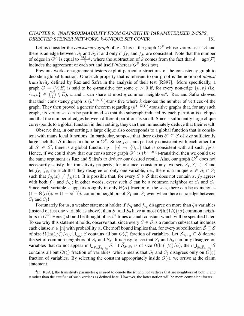
CHAPTER 9. INAPPROXIMABILITY FROM GAP-ETH III: PARAMETERIZED 2-CSPS,DIRECTED STEINER NETWORK, k-UNIQUE SET COVER 161
Let us consider the consistency graph of F . This is the graph GF whose vertex set is S andthere is an edge between S1 and S2 if and only if fS1 and fS2 are consistent. Note that the numberof edges in GF is equal to k2δ−k
2 , where the subtraction of k comes from the fact that δ = agr(F)includes the agreement of each set and itself (whereas GF does not).
Previous works on agreement testers exploit particular structures of the consistency graph todecode a global function. One such property that is relevant to our proof is the notion of almosttransitivity defined by Raz and Safra in the analysis of their test [RS97]. More specifically, agraph G = (V,E) is said to be q-transitive for some q > 0 if, for every non-edge u, v (i.e.u, v ∈
(V2
)\ E), u and v can share at most q common neighbors4. Raz and Safra showed
that their consistency graph is (k1−Ω(1))-transitive where k denotes the number of vertices of thegraph. They then proved a generic theorem regarding (k1−Ω(1))-transitive graphs that, for any suchgraph, its vertex set can be partitioned so that the subgraph induced by each partition is a cliqueand that the number of edges between different partitions is small. Since a sufficiently large cliquecorresponds to a global function in their setting, they can then immediately deduce that their result.
Observe that, in our setting, a large clique also corresponds to a global function that is consis-tent with many local functions. In particular, suppose that there exists S ′ ⊆ S of size sufficientlylarge such that S induces a clique in GF . Since fS′’s are perfectly consistent with each other forall S ′ ∈ S ′, there is a global function g : [n] → 0, 1 that is consistent with all such fS′’s.Hence, if we could show that our consistency graph GF is (k1−Ω(1))-transitive, then we could usethe same argument as Raz and Safra’s to deduce our desired result. Alas, our graph GF does notnecessarily satisfy this transitivity property; for instance, consider any two sets S1, S2 ∈ S andlet fS1 , fS2 be such that they disagree on only one variable, i.e., there is a unique x ∈ S1 ∩ S2such that fS1(x) 6= fS2(x). It is possible that, for every S ∈ S that does not contain x, fS agreeswith both fS1 and fS2; in other words, every such S can be a common neighbor of S1 and S2.Since each variable x appears roughly in only Θ(α) fraction of the sets, there can be as many as(1−Θ(α))k = (1− o(1))k common neighbors of S1 and S2 even when there is no edge betweenS1 and S2!
Fortunately for us, a weaker statement holds: if fS1 and fS2 disagree on more than ζn variables(instead of just one variable as above), then S1 and S2 have at most O(ln(1/ζ)/α) common neigh-bors in GF . Here ζ should be thought of as β2 times a small constant which will be specified later.To see why this statement holds, observe that, since every S ∈ S is a random subset that includeseach clause x ∈ [n] with probability α, Chernoff bound implies that, for every subcollection S ⊆ Sof size Ω(ln(1/ζ)/α),
⋃S∈S S contains all but O(ζ) fraction of variables. Let SS1,S2 ⊆ S denote
the set of common neighbors of S1 and S2. It is easy to see that S1 and S2 can only disagree onvariables that do not appear in
⋃S∈SS1,S2
S. If SS1,S2 is of size Ω(ln(1/ζ)/α), then⋃S∈SS1,S2
S
contains all but O(ζ) fraction of variables, which means that S1 and S2 disagrees only on O(ζ)fraction of variables. By selecting the constant appropriately inside O(·), we arrive at the claimstatement.
4In [RS97], the transitivity parameter q is used to denote the fraction of vertices that are neighbors of both u andv rather than the number of such vertices as defined here. However, the latter notion will be more convenient for us.
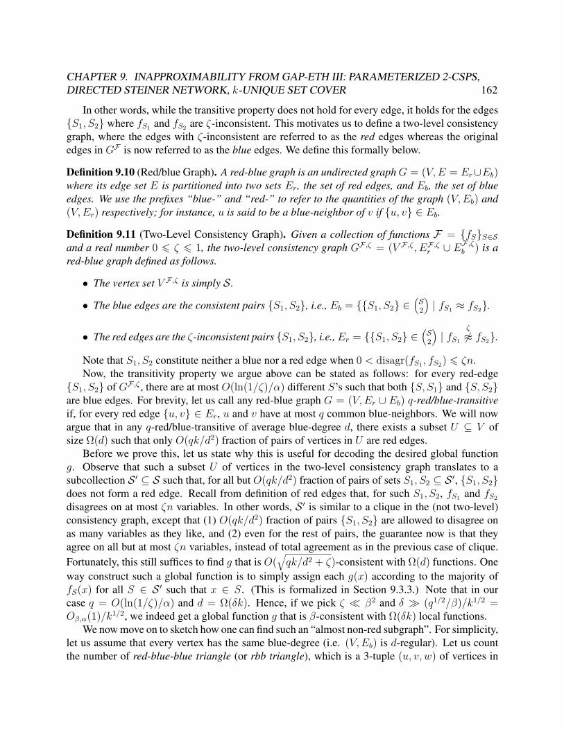
CHAPTER 9. INAPPROXIMABILITY FROM GAP-ETH III: PARAMETERIZED 2-CSPS,DIRECTED STEINER NETWORK, k-UNIQUE SET COVER 162
In other words, while the transitive property does not hold for every edge, it holds for the edgesS1, S2 where fS1 and fS2 are ζ-inconsistent. This motivates us to define a two-level consistencygraph, where the edges with ζ-inconsistent are referred to as the red edges whereas the originaledges in GF is now referred to as the blue edges. We define this formally below.
Definition 9.10 (Red/blue Graph). A red-blue graph is an undirected graphG = (V,E = Er∪Eb)where its edge set E is partitioned into two sets Er, the set of red edges, and Eb, the set of blueedges. We use the prefixes “blue-” and “red-” to refer to the quantities of the graph (V,Eb) and(V,Er) respectively; for instance, u is said to be a blue-neighbor of v if u, v ∈ Eb.
Definition 9.11 (Two-Level Consistency Graph). Given a collection of functions F = fSS∈Sand a real number 0 6 ζ 6 1, the two-level consistency graph GF ,ζ = (V F ,ζ , EF ,ζr ∪ EF ,ζb ) is ared-blue graph defined as follows.
• The vertex set V F ,ζ is simply S.
• The blue edges are the consistent pairs S1, S2, i.e., Eb = S1, S2 ∈(S2
)| fS1 ≈ fS2.
• The red edges are the ζ-inconsistent pairs S1, S2, i.e.,Er = S1, S2 ∈(S2
)| fS1
ζ
6≈ fS2.
Note that S1, S2 constitute neither a blue nor a red edge when 0 < disagr(fS1 , fS2) 6 ζn.Now, the transitivity property we argue above can be stated as follows: for every red-edge
S1, S2 of GF ,ζ , there are at most O(ln(1/ζ)/α) different S’s such that both S, S1 and S, S2are blue edges. For brevity, let us call any red-blue graph G = (V,Er ∪ Eb) q-red/blue-transitiveif, for every red edge u, v ∈ Er, u and v have at most q common blue-neighbors. We will nowargue that in any q-red/blue-transitive of average blue-degree d, there exists a subset U ⊆ V ofsize Ω(d) such that only O(qk/d2) fraction of pairs of vertices in U are red edges.
Before we prove this, let us state why this is useful for decoding the desired global functiong. Observe that such a subset U of vertices in the two-level consistency graph translates to asubcollection S ′ ⊆ S such that, for all but O(qk/d2) fraction of pairs of sets S1, S2 ⊆ S ′, S1, S2does not form a red edge. Recall from definition of red edges that, for such S1, S2, fS1 and fS2
disagrees on at most ζn variables. In other words, S ′ is similar to a clique in the (not two-level)consistency graph, except that (1) O(qk/d2) fraction of pairs S1, S2 are allowed to disagree onas many variables as they like, and (2) even for the rest of pairs, the guarantee now is that theyagree on all but at most ζn variables, instead of total agreement as in the previous case of clique.Fortunately, this still suffices to find g that is O(
√qk/d2 + ζ)-consistent with Ω(d) functions. One
way construct such a global function is to simply assign each g(x) according to the majority offS(x) for all S ∈ S ′ such that x ∈ S. (This is formalized in Section 9.3.3.) Note that in ourcase q = O(ln(1/ζ)/α) and d = Ω(δk). Hence, if we pick ζ β2 and δ (q1/2/β)/k1/2 =Oβ,α(1)/k1/2, we indeed get a global function g that is β-consistent with Ω(δk) local functions.
We now move on to sketch how one can find such an “almost non-red subgraph”. For simplicity,let us assume that every vertex has the same blue-degree (i.e. (V,Eb) is d-regular). Let us countthe number of red-blue-blue triangle (or rbb triangle), which is a 3-tuple (u, v, w) of vertices in
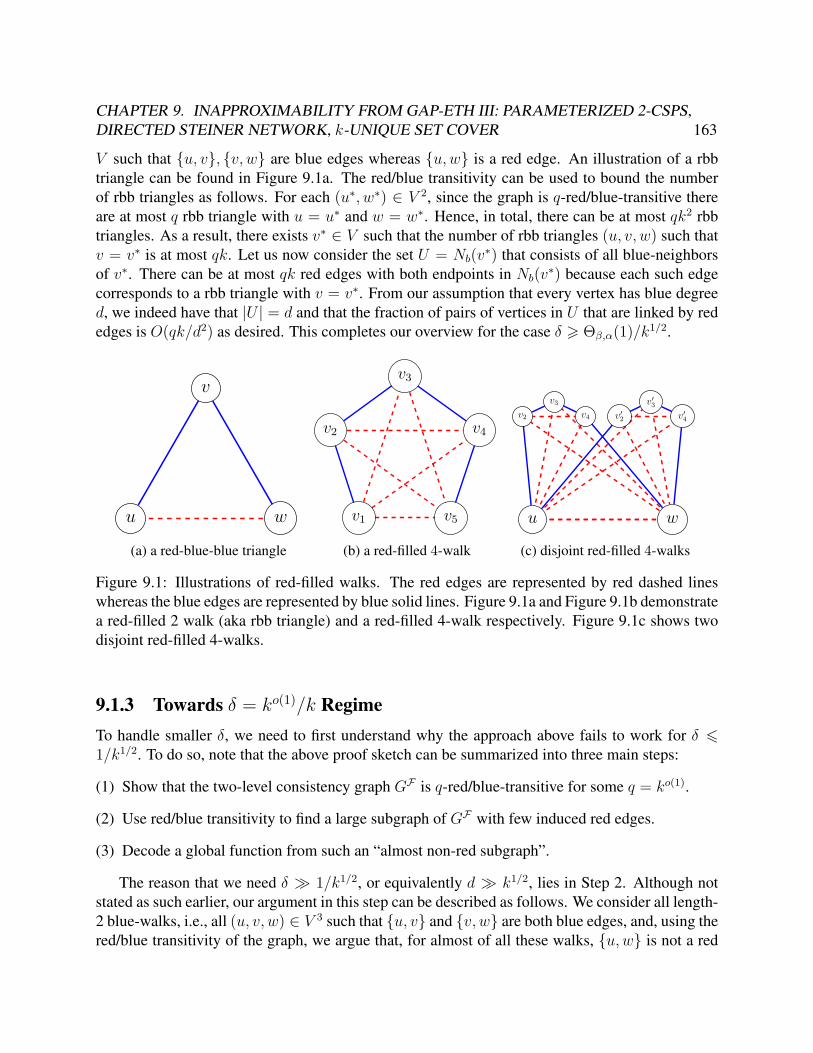
CHAPTER 9. INAPPROXIMABILITY FROM GAP-ETH III: PARAMETERIZED 2-CSPS,DIRECTED STEINER NETWORK, k-UNIQUE SET COVER 163
V such that u, v, v, w are blue edges whereas u,w is a red edge. An illustration of a rbbtriangle can be found in Figure 9.1a. The red/blue transitivity can be used to bound the numberof rbb triangles as follows. For each (u∗, w∗) ∈ V 2, since the graph is q-red/blue-transitive thereare at most q rbb triangle with u = u∗ and w = w∗. Hence, in total, there can be at most qk2 rbbtriangles. As a result, there exists v∗ ∈ V such that the number of rbb triangles (u, v, w) such thatv = v∗ is at most qk. Let us now consider the set U = Nb(v∗) that consists of all blue-neighborsof v∗. There can be at most qk red edges with both endpoints in Nb(v∗) because each such edgecorresponds to a rbb triangle with v = v∗. From our assumption that every vertex has blue degreed, we indeed have that |U | = d and that the fraction of pairs of vertices in U that are linked by rededges is O(qk/d2) as desired. This completes our overview for the case δ > Θβ,α(1)/k1/2.
u
v
w
(a) a red-blue-blue triangle
v1
v2
v3
v4
v5
(b) a red-filled 4-walk
u w
v2
v3
v4 v′2
v′3v′4
(c) disjoint red-filled 4-walks
Figure 9.1: Illustrations of red-filled walks. The red edges are represented by red dashed lineswhereas the blue edges are represented by blue solid lines. Figure 9.1a and Figure 9.1b demonstratea red-filled 2 walk (aka rbb triangle) and a red-filled 4-walk respectively. Figure 9.1c shows twodisjoint red-filled 4-walks.
9.1.3 Towards δ = ko(1)/k RegimeTo handle smaller δ, we need to first understand why the approach above fails to work for δ 61/k1/2. To do so, note that the above proof sketch can be summarized into three main steps:
(1) Show that the two-level consistency graph GF is q-red/blue-transitive for some q = ko(1).
(2) Use red/blue transitivity to find a large subgraph of GF with few induced red edges.
(3) Decode a global function from such an “almost non-red subgraph”.
The reason that we need δ 1/k1/2, or equivalently d k1/2, lies in Step 2. Although notstated as such earlier, our argument in this step can be described as follows. We consider all length-2 blue-walks, i.e., all (u, v, w) ∈ V 3 such that u, v and v, w are both blue edges, and, using thered/blue transitivity of the graph, we argue that, for almost of all these walks, u,w is not a red
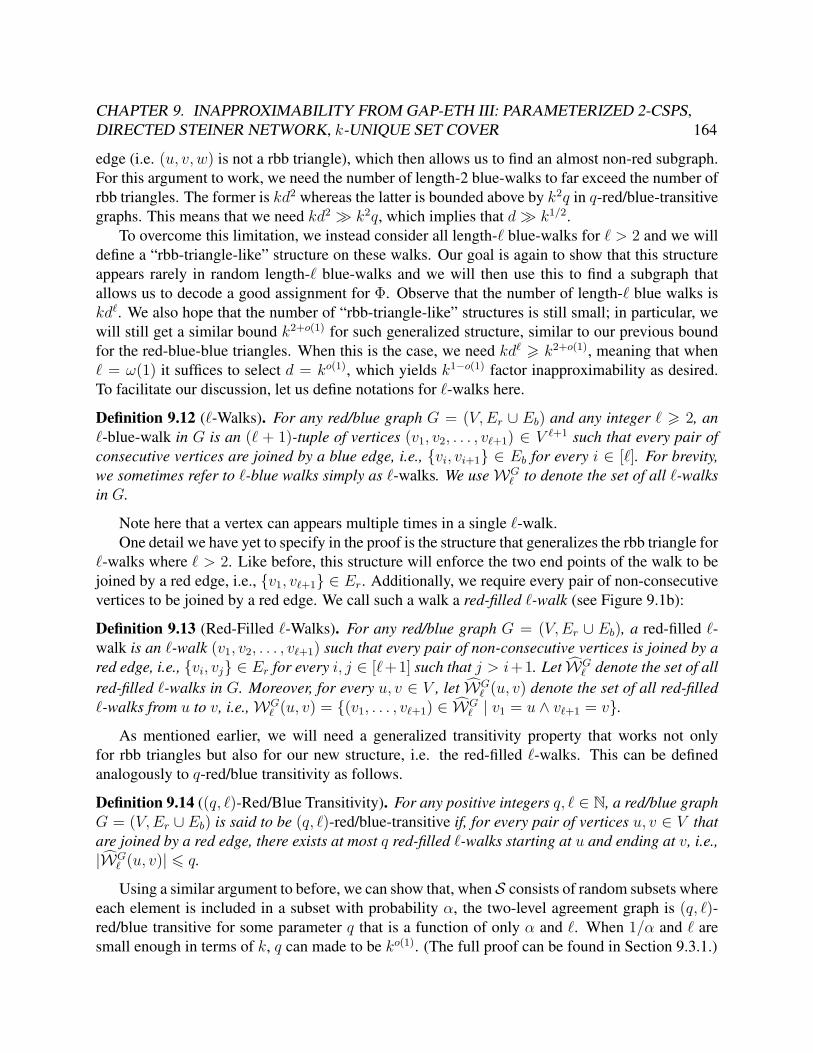
CHAPTER 9. INAPPROXIMABILITY FROM GAP-ETH III: PARAMETERIZED 2-CSPS,DIRECTED STEINER NETWORK, k-UNIQUE SET COVER 164
edge (i.e. (u, v, w) is not a rbb triangle), which then allows us to find an almost non-red subgraph.For this argument to work, we need the number of length-2 blue-walks to far exceed the number ofrbb triangles. The former is kd2 whereas the latter is bounded above by k2q in q-red/blue-transitivegraphs. This means that we need kd2 k2q, which implies that d k1/2.
To overcome this limitation, we instead consider all length-` blue-walks for ` > 2 and we willdefine a “rbb-triangle-like” structure on these walks. Our goal is again to show that this structureappears rarely in random length-` blue-walks and we will then use this to find a subgraph thatallows us to decode a good assignment for Φ. Observe that the number of length-` blue walks iskd`. We also hope that the number of “rbb-triangle-like” structures is still small; in particular, wewill still get a similar bound k2+o(1) for such generalized structure, similar to our previous boundfor the red-blue-blue triangles. When this is the case, we need kd` > k2+o(1), meaning that when` = ω(1) it suffices to select d = ko(1), which yields k1−o(1) factor inapproximability as desired.To facilitate our discussion, let us define notations for `-walks here.
Definition 9.12 (`-Walks). For any red/blue graph G = (V,Er ∪ Eb) and any integer ` > 2, an`-blue-walk in G is an (` + 1)-tuple of vertices (v1, v2, . . . , v`+1) ∈ V `+1 such that every pair ofconsecutive vertices are joined by a blue edge, i.e., vi, vi+1 ∈ Eb for every i ∈ [`]. For brevity,we sometimes refer to `-blue walks simply as `-walks. We useWG
` to denote the set of all `-walksin G.
Note here that a vertex can appears multiple times in a single `-walk.One detail we have yet to specify in the proof is the structure that generalizes the rbb triangle for
`-walks where ` > 2. Like before, this structure will enforce the two end points of the walk to bejoined by a red edge, i.e., v1, v`+1 ∈ Er. Additionally, we require every pair of non-consecutivevertices to be joined by a red edge. We call such a walk a red-filled `-walk (see Figure 9.1b):
Definition 9.13 (Red-Filled `-Walks). For any red/blue graph G = (V,Er ∪ Eb), a red-filled `-walk is an `-walk (v1, v2, . . . , v`+1) such that every pair of non-consecutive vertices is joined by ared edge, i.e., vi, vj ∈ Er for every i, j ∈ [`+1] such that j > i+1. Let WG
` denote the set of allred-filled `-walks in G. Moreover, for every u, v ∈ V , let WG
` (u, v) denote the set of all red-filled`-walks from u to v, i.e.,WG
` (u, v) = (v1, . . . , v`+1) ∈ WG` | v1 = u ∧ v`+1 = v.
As mentioned earlier, we will need a generalized transitivity property that works not onlyfor rbb triangles but also for our new structure, i.e. the red-filled `-walks. This can be definedanalogously to q-red/blue transitivity as follows.
Definition 9.14 ((q, `)-Red/Blue Transitivity). For any positive integers q, ` ∈ N, a red/blue graphG = (V,Er ∪ Eb) is said to be (q, `)-red/blue-transitive if, for every pair of vertices u, v ∈ V thatare joined by a red edge, there exists at most q red-filled `-walks starting at u and ending at v, i.e.,|WG
` (u, v)| 6 q.
Using a similar argument to before, we can show that, when S consists of random subsets whereeach element is included in a subset with probability α, the two-level agreement graph is (q, `)-red/blue transitive for some parameter q that is a function of only α and `. When 1/α and ` aresmall enough in terms of k, q can made to be ko(1). (The full proof can be found in Section 9.3.1.)
CHAPTER 9. INAPPROXIMABILITY FROM GAP-ETH III: PARAMETERIZED 2-CSPS,DIRECTED STEINER NETWORK, k-UNIQUE SET COVER 165
Once this is proved, it is not hard (using a similar argument as before) to show that, whend (kq)1/`, most `-walks are not red-filled, i.e., |WG
` | |WG` |. Even with this, it is still unclear
how we can get back a “clique-like” subgraph; in the case of ` = 2 above, this implies that ablue-neighborhood induces few red edges, but the argument does not seem to generalize to larger`. Fortunately, it is still quite easy to find a large subgraph that a non-trivial fraction of pairs ofvertices do not form red edges; specifically, we will find two subsets U1, U2 ⊆ V each of size dsuch that for at least 1/`2 fraction of (u1, u2) ∈ U1 × U2, u1, u2 is not a red edge. To find suchsets, observe that, if |WG
` | > 2|WG` |, then for a random (v1, . . . , v`+1) ∈ WG
` the probability thatthere exists non-consecutive vertex vi, vj in the walk that are joined by a red edge is at least 1/2.Since there are less than `2/2 such i, j, union bound implies that there must be non-consecutivei∗, j∗ such that the probability that vi∗ , vj∗ are not joined by a red edge is at least 1/`2. Let usassume without loss of generality that i∗ < j∗; since they are not consecutive, we have i∗+1 < j∗.
Let us consider vi∗+1, vj∗−1. By a simple averaging argument, there must be u∗ and w∗ suchthat, conditioning on vi∗+1 = u∗ and vj∗+1 = w∗, the probability that vi∗ , vj∗ /∈ Er is at least1/`2. However, this conditional probability is exactly equal to fraction of (u1, u2) ∈ Nb(u∗) ×Nb(w∗) that u1 and u2 are not joined by a red edge. Recall again that Nb(v) is used to denote theset of all blue-neighbors of v. Thus, U1 = Nb(u∗) and U2 = Nb(w∗) are the sets with desiredproperty.
We are still not done yet since we have to use these sets to decode back the global function g.This is still not obvious: the guarantee we have for our sets U1, U2 is rather weak since we onlyknow that at least 1/`2 of the pairs of vertices from the two sets do not form red edges. This is incontrast to the ` = 2 case where we have a subgraph such that almost all induced edges are notred.
To see how to overcome this barrier, recall that a pair S1, S2 that does not form a red edge
corresponds to fS1
ζ≈ fS2 . As a thought experiment, let us think of the following scenario: if
instead of just ζ-consistency, these pairs satisfy (exact) consistency, then we can consider thecollection F = fSS∈U where U = U1∪U2. This is a collection of Θ(d) local functions such thatagr(F) > Ω(1/`2). Thus, when d `4, we are in the regime where agr(F) 1/d1/2, meaningthat we can apply our earlier argument (for the δ > ko(1)/k1/2 regime) to recover g!
The approach in the previous paragraph of course does not work directly because we only knowthat Ω(1/`2) fraction of the pairs S1, S2 ⊆ U are ζ-consistent, not exactly consistent. However,we can still try to mimic the proof in the regime δ > ko(1)/k1/2 and define a red/blue graph insuch a way that such ζ-consistent pairs are now blue edges. Naturally, the red edges will now bethe ζ ′-inconsistent pairs for some ζ ′ > ζ . In other words, we consider the generalized two-levelconsistency graph defined as follows.
Definition 9.15 (Generalized Two-Level Consistency Graph). Given a collection of functions F =fSS∈S and two real numbers 0 6 ζ 6 ζ ′ 6 1, the generalized two-level consistency graphGF ,ζ,ζ
′ = (V F ,ζ,ζ′ , EF ,ζ,ζ′r ∪ EF ,ζ,ζ′
b ) is a red/blue graph defined as follows.
• The vertex set V F ,ζ,ζ′
is simply S.
CHAPTER 9. INAPPROXIMABILITY FROM GAP-ETH III: PARAMETERIZED 2-CSPS,DIRECTED STEINER NETWORK, k-UNIQUE SET COVER 166
• The blue edges are the ζ-consistent pairs S1, S2, i.e., EF ,ζ,ζ′
b = S1, S2 ∈(S2
)| fS1
ζ≈
fS2.
• The red edges are the ζ ′-inconsistent pairs S1, S2, i.e., EF ,ζ,ζ′
r = S1, S2 ∈(S2
)| fS1
ζ′
6≈fS2.
As its name suggests, the generalized two-level consistency graph is a generalization of thetwo-level consistency graph from Definition 9.11; namely GF ,0,ζ in the more general definitioncoincides with GF ,ζ in the original definition.
Now, it is not hard to show that when ζ ′ ζ/α, the graph GF ,ζ,ζ′ is again q-red/blue transitivefor some q that depends only on α and ζ . This means that we can apply our argument from theδ > 1/k1/2−o(1) regime on the graphGF ,ζ,ζ′ , which yields a subset U ⊆ U such that almost all pairsS1, S2 ⊆ U are ζ ′-consistent. By selecting the parameters appropriately, such an almost non-redsubgraph once again gives us the desired global function. This wraps up our proof overview.
9.2 Additional Preliminaries
9.2.1 Parameters of Well-Behaved SubsetsWe next recall two properties of collections of subsets, which will be needed in our soundnessanalysis. First, recall that, in our proof overview for the weaker k1/2−o(1) factor hardness, we needthe following to show the red/blue transitivity of the consistency graph: for any r subsets from thecollection, their union must contain almost all clauses. Here r is a positive integer that effects thered/blue transitivity parameter. This coincides with the definition of dispersers (Definition 2.20).For walks with larger length, we need a stronger property that any union of r intersections of `subsets are large. Recall that this is exactly the notion of intersection dispersers in Definition 2.21.
Another property we need is that any sufficiently large subcollection S of S is “sufficientlyuniform” in the sense of Definition 2.18. More specifically, recall that the uniformity conditionrequires that almost all clauses appear in not too small number of subsets in S. This is used whenwe decode a good assignment from an almost non-red subgraph.
Using standard concentration bounds, it is not hard to show that, when m is sufficiently large,a collection of random subsets where each element is included in each subset independentlywith probability α is an (1/O(α`), `, O(1))-disperser and every subcollection of size Ω(1/α) is(α,O(1)) uniform. This can be easily derandomized using the construction from Section 2.9, asstated formally below.
Lemma 9.16 (Deterministic Construction of Well-Behaved Subsets). For any k, `, q ∈ N and anyinteger m > qk+1, let U be any m-element set. Then, there is a collection T of k subsets of U withthe following properties with α := 1/q.
• (Size) Every subset in T has size at most 2αm.
CHAPTER 9. INAPPROXIMABILITY FROM GAP-ETH III: PARAMETERIZED 2-CSPS,DIRECTED STEINER NETWORK, k-UNIQUE SET COVER 167
• (Intersection Disperser) For any η > 0, T is a (dln(1/η)/α`e, `, η)-intersection disperser.
• (Uniformity) For any µ > 0, any subcollection T ⊆ T of size d8 ln(1/µ)/αe is (α/2, µ)-uniform.
Moreover, such a collection T can be deterministically constructed in time O(m · qk).
Proof. Let z = bm/qkc. To define the sets, we first partition U into two parts U0,U1, where U0 isof size qk · z and U1 is of size m − |U0| < qk. We associate the elements of U0 with [q]k × [z].Let T1, . . . , Tk be the sets as in Definition 2.16 with t = 1. We define the set T ′1, . . . , T
′k ⊆ U by
T ′i = (Ti × [z]) ∪ U1. The intersection disperser property and uniformity of T = T ′1, . . . , T ′kfollows immediately from Propositions 2.22 and 2.19 respectively. Finally, each set is of size atmost qk−1 · z + qk 6 2αm, where the inequality comes from our assumption that m > qk+1.
Let us turn our focus back to our main technical contribution: the agreement testing theorem.
9.3 The Main Agreement TheoremThe main goal of this section is to prove the following agreement theorem, which is the formalversion of Theorem 9.9 and is also the main technical contribution of this chapter.
Theorem 9.17. For any 0 < η, ζ, γ, µ < 1 and r, `, k, h, n, d ∈ N such that ` > 2, let S be anycollection of k subsets of [n] such that S is (r, `, ζ)-intersection disperser and every subcollectionS ⊆ S of size h is (γ, µ)-uniform, and let F = fSS∈S be any collection of functions. Ifδ := agr(F) > 10+64(r`)2k1/`
k, then there exists a subcollection S ′ ⊆ S of size at least δk
256`2
and a function g : [n]→ 0, 1 such that gβ≈ fS for all S ∈ S ′ where
β = 2√
65536h`6
δk+ µ+ 2ζ/γ.
While the parameters of the theorem can be confusing, when each subset in S is a randomαn-size subset of [n], the parameters we are interested in are as follows: µ and η both go to 0 asn goes to infinity, h and γ depend only on α, and, r is O(1/α`). Since we want the requirementon soundness as weak as possible, we want to minimize (r`)2k1/` = 2Oα(`+(log k)/`). Hence, ourbest choice is to let ` =
√log k, which indeed yields the k/2(log k)1/2+ρ ratio inapproximability for
2-CSPs.To prove this theorem, we follow the general outline as stated in the proof overview section. In
particular, the proof contains five main steps, as elaborated below.
(1) First, we will show that when S is an intersection disperser with appropriate parameters, thenthe two-level consistency graph GF ,ζ satisfies (q, `)-red/blue transitivity for certain q, `.
CHAPTER 9. INAPPROXIMABILITY FROM GAP-ETH III: PARAMETERIZED 2-CSPS,DIRECTED STEINER NETWORK, k-UNIQUE SET COVER 168
(2) Second, we argue that, for any red/blue transitive graphs that contains sufficiently many blueedges, we can find a large subset U of vertices such that a reasonably large fraction of pairsS1, S2 ⊆ U are non-red. This is done by counting red-filled `-walks for an appropriate `.
(3) We then focus on F = fSU and show, using a uniformity condition of S, that the generalizedtwo-level consistency graph GF ,ζ,ζ′ is red/blue transitive with certain parameters.
(4) Next, counting rbb triangles reveals a large “almost non-red subgraph” in the graph GF ,ζ,ζ′ .
(5) Finally, we decode a global function from this almost non-red subgraph.
This section is organized as follows. In Subsection 9.3.1, we show transitivity properties ofthe two-level and generalized two-level consistency graphs, i.e., Steps 1 and 3. Subsection 9.3.2contains a structural lemma regarding an existence of a large subgraph with certain non-red densityin red/blue transitive graphs; this lemma is at the heart of Steps 2 and 4. Next, in Subsection 9.3.3,we prove Step 5. Finally, in Subsection 9.3.4, we put these parts together and prove Theorem 9.17.
9.3.1 Red/Blue-Transitivity of (Generalized) Two-Level Consistency GraphRed/Blue-Transitivity from Intersection Disperser
The first step in our proof is to show that the two-level consistency graphGF ,ζ is red/blue-transitive,assuming that S is an intersection disperser. Specifically, our main lemma is the following:
Lemma 9.18. If S is an (r, `, ζ)-intersection disperser, then, for any F = fSS∈S , GF ,ζ is((r`)2(`−1), `)-red/blue-transitive.
We note here that both in Lemma 9.18 and Claim 9.19 below, the transitivity property holds notonly for `-walks as specified in the statements, but also for (`+ 1)-walks. However, since the latterdoes not yield any improvement to our main results, we work with only `-walks, which makes thecalculations cleaner.
In other words, we would like to show that, for every S1, S2 ∈ S that are joined by a red edge inGF ,ζ , there are at most (r`)2(`−1) red-filled `-walks from S1 to S2. The intersection disperser doesnot immediately imply such a bound, due to the requirement in the definition that the subcollectionsare disjoint. Rather, it only directly implies a bound on number of disjoint `-walks from S1 to S2,where two ` walks from S1 to S2, (T1 = S1, . . . , T`+1 = S2), (T ′1 = S1, . . . , T
′`+1 = S2) ∈
WGF,ζ` (S1, S2), are said to be disjoint if they do not share any vertex except the starting and ending
vertices, i.e., T2, . . . , T`∩T ′2, . . . , T ′` = ∅. Note that multiple walks sharing starting and endingvertices are said to be disjoint if they are mutually disjoint. The following claim follows almostimmediately from definition of intersection dispersers:
Claim 9.19. If S is an (r, `, ζ)-intersection disperser, then, for any F = fSS∈S , any integer2 6 p 6 ` and any S1, S2 ∈ EF ,ζr , there are less than r disjoint p-walks from S1 to S2 in GF ,ζ .
CHAPTER 9. INAPPROXIMABILITY FROM GAP-ETH III: PARAMETERIZED 2-CSPS,DIRECTED STEINER NETWORK, k-UNIQUE SET COVER 169
Proof. Suppose for the sake of contradiction that S is an (r, `, ζ)-intersection disperser but thereexist F = fSS∈S , 2 6 p 6 ` and S1, S2 ∈ EF ,ζr such that there are at least r disjoint p-walks from S1 to S2. Let these walks be (T1,1 = S1, T1,2, . . . , T1,p, T1,p+1 = S2), . . . , (Tr,1 =S1, Tr,2, . . . , Tr,p, Tr,p+1 = S2) ∈ WGF,ζ
p (S1, S2).For each i ∈ [r], consider any x ∈ ⋂p+1
j=1 Ti,j . Apriori this intersection may be empty but sinceS is an intersection disperser this usually does not occur. Since Ti,j, Ti,j+1 ∈ EF ,ζb for everyj ∈ [p], we have
fS1(x) = fTi,1(x) = fTi,2(x) = · · · = fTi,p(x) = fTi,p+1(x) = fS2(x).
Hence, for every x ∈ ⋃ri=1
(⋂p+1j=1 Tq,j
), fS1(x) = fS2(x). Let T ∗ denote
⋃ri=1
(⋂pj=2 Tq,j
).
Since Ti,1 = S1 and Ti,p+1 = S2 for all i ∈ [r], we have
r⋃i=1
p+1⋂j=1
Tq,j
= (S1 ∩ S2) ∩ T ∗.
In other words, fS1 and fS2 can only disagree on variables outside of T ∗. However, since S isan (r, `, ζ)-intersection disperser, we have |T ∗| > (1 − ζ)n. Hence, disagr(S1, S2) 6 ζn, whichcontradicts with S1, S2 ∈ EF ,ζr .
Since all 2-walks from S1 to S2 are disjoint, the above claim immediately gives a bound onthe number of red-filled 2-walks from S1 to S2. To bound the number of red-filled walks of largerlengths, we will use induction on the length of the walks. Suppose that we have bounded thenumber of red-filled i-walks sharing starting and ending vertices for i 6 z− 1. The key idea in theproof is that we can use this inductive hypothesis to show that, for any S1, S2, S ∈ S, few z-walksfrom S1 to S2 contain a given S. Here we say that a z-walk (T1 = S1, . . . , Tz = S2) from S1 to S2contains S if S ∈ T2, . . . , Tz. This implies that for a given z-walk from S1 to S2 there are onlyfew walks that are not disjoint from it. This allows us to show that, if there are too many z-walks,then there must also be many disjoint z-walks as well, which would violate Claim 9.19. A formalproof of Lemma 9.18 based on this intuition is given below.
Proof of Lemma 9.18. For every integer i such that 2 6 i 6 `, let P (i) denote the followingstatement: for every S1, S2 ∈ S, |WGF,ζ
i (S1, S2)| 6 (ri)2(i−1). For convenience, letBi = (ri)2(i−1)
for every 2 6 i 6 `.Base Case. Since every different 2-walks from S1 to S2 are disjoint, Claim 9.19 immediately
implies that the number of 2-walks from S1 to S2 is at most r 6 B2.Inductive Step.Suppose that, for some integer z such that 3 6 z 6 `, P (3), . . . , P (z − 1) are true. We will
show that P (z) is true. To do so, let us first prove that, for any fixed starting and ending vertices,any vertex cannot appears in too many red-filled z-walks, as stated in the following claim.
Claim 9.20. For all S1, S2, S ∈ S , the number of red-filled z-walks from S1 to S2 containing S inGF ,ζ is at most Bz/(zr).
CHAPTER 9. INAPPROXIMABILITY FROM GAP-ETH III: PARAMETERIZED 2-CSPS,DIRECTED STEINER NETWORK, k-UNIQUE SET COVER 170
Proof. First, observe that the number of red-filled z-walks from S1 to S2 containing S is at mostthe sum over all positions 2 6 j 6 z of the number of z-walks from S1 to S2 such that the j-thvertex in the walk is S. More formally, the number of red-filled z-walks from S1 to S2 containingS is
|(T1, . . . , Tz+1) ∈ WGF,ζ
z (S1, S2) | ∃2 6 j 6 z, Tj = Sj| 6z∑j=2|(T1, . . . , Tz+1) ∈ WGF,ζ
z (S1, S2) | Tj = S|.
Now, for each 2 6 j 6 z, to bound the number of red-filled z-walks from S1 to S2 whose j-thvertex is S, let us consider the following three cases based on the value of j:
1. 3 6 j 6 z − 1. Observe that, for any such walk (T1 = S1, T2, . . . , Tj = S, . . . , Tz, Tz+1 =S2), the subwalk (T1 = S1, . . . , Tj = S) and (Tj = S, . . . , Tz+1 = S2) must be red-filledwalks as well. Since the numbers of red-filled (j − 1)-walks from S1 to S and red-filled(z + 1 − j)-walks from S to S2 are bounded by Bj−1 and Bz+1−j respectively (from theinductive hypothesis), there are at most Bj−1 choices of (T1 = S1, . . . , Tj = S) and Bz+1−jchoices of (Tj = S, . . . , Tz−1, Tz = S2). Hence, there are at most Bj−1Bz+1−j red-filledz-walks from S1 to S2 whose j-th vertex is S.
2. j = 2. In this case, the subwalk (Tj = S, . . . , Tz+1 = S2) must be a red-filled (z − 1)-walkfrom S to S2. Hence, the number of red-filled z-walks from S1 to S2 where Tj = S isbounded above by Bz−1.
3. j = z. Similar to the previous case, we also have the bound of Bz−1.
For convenience, let B1 = 1. The above argument gives us the following bound for every 2 6 j 6z:
|(T1, . . . , Tz+1) ∈ WGF,ζ
z (S1, S2) | Tj = S| 6 Bj−1Bz+1−j.
Summing this over j, we have the following upper bound on the number of red-filled z-walksfrom S1 to S2 containing S:
z∑j=2
Bj−1Bz+1−j =z∑j=2
(r(j − 1))2(j−2)(r(z + 1− j))2(z−j) 6z∑j=2
(rz)2(z−2) 6 Bz/(zr),
which concludes the proof of the claim. y
Having proved the above claim, it is now easy to show that P (z) is true. Suppose for the sake ofcontradiction that there exists S1, S2 ∈ S such that |WGF,ζ
z (S1, S2)| > Bz. Consider the followingprocedure of selecting disjoint walks from WGF,ζ
z (S1, S2). First, initialize U = WGF,ζz (S1, S2) and
repeat the following process as long as U 6= ∅: select any (T1, . . . , Tz+1) ∈ U and remove every(T ′1, . . . , T ′z+1) that is not disjoint with (T1, . . . , Tz+1) from U . Observe that, each time a walk(T1, . . . , Tz+1) is selected, the number of walks removed from U is at most Bz/r; this is becauseeach removed walk must contain at least one of T2, . . . , Tz, but, from the above claim, each of
CHAPTER 9. INAPPROXIMABILITY FROM GAP-ETH III: PARAMETERIZED 2-CSPS,DIRECTED STEINER NETWORK, k-UNIQUE SET COVER 171
these vertices are contained in at most Bz/(zr) walks. Since we start with more than Bz walks, atleast r walks are picked. These walks are disjoint z-walks starting from S1 and S2, which, due toClaim 9.19, is a contradiction. Thus, P (z) is true as desired.
Hence, P (`) is true, which, by definition, implies that GF is ((r`)2(`−1), `)-red/blue-transitive.
Red/Blue-Transitivity from Uniformity
In Step 3 of our proof, we need to show red/blue-transitivity of the generalized two-level consis-tency graph GF ,ζ,ζ′ . This is encapsulated in the following lemma.
Lemma 9.21. If every subcollection S ⊆ S of size r is (γ, µ)-uniform, then, for any ζ > 0,ζ ′ > µ+2ζ/γ and F = fSS∈S , the generalized two-level consistency graphGF ,ζ,ζ
′is r-red/blue
transitive.
The proof of the lemma is quite simple. The key observation is that, if S1 and S2 are joinedby a red edge and T is a common blue-neighbor in the graph GF ,ζ,ζ′ , then it means that T onlyhits a small number (i.e. 2ζn) of the variables on which fS1 and fS2 disagree. In other words,such variables appear less frequently in common blue-neighbors of S1 and S2. If the common-blueneighbor set is of size r, this contradicts the fact that the set is (γ, µ)-uniform. This intuition isformalized below.
Proof of Lemma 9.21. Suppose for the sake of contradiction thatGF ,ζ,ζ′ is not r-red/blue transitive.That is, there exist S1, S2 ∈ S that are joined by a red edge such that there are r red-filled 2-walks(i.e. rbb triangle) from S1 to S2. Suppose that these walks are (S1, T1, S2), (S1, T2, S2), · · · , (S1, Tr, S2).
For every i ∈ [r], since (S1, Ti, S2) is a 2-walk, S1, Ti and S2, Ti are blue edges. Thisimplies that
disagr(fS1 , fTi), disagr(fS2 , fTi) 6 ζn. (9.1)
On the other hand, we can lower bound Ei∈[r][disagr(fS1 , fTi) + disagr(fS2 , fTi)] as follows.First, let let Xdisagr denote the set of all x ∈ S1 ∩ S2 such that fS1(x) 6= fS2(x); since S1, S2 is ared edge, we have |Xdisagr| > ζ ′n. We can rearrange Ei∈[r][disagr(fS1 , fTi) + disagr(fS2 , fTi)] as
Ei∈[r][disagr(fS1 , fTi) + disagr(fS2 , fTi)]
=∑x∈[n]
(Pri∈[r]
[x ∈ (S1 ∩ Ti) ∧ fS1(x) 6= fTi(x)] + Pri∈[r]
[x ∈ (S2 ∩ Ti) ∧ fS2(x) 6= fTi(x)])
>∑
x∈Xdisagr
(Pri∈[r]
[x ∈ Ti ∧ fS1(x) 6= fTi(x)] + Pri∈[r]
[x ∈ Ti ∧ fS2(x) 6= fTi(x)])
>∑
x∈Xdisagr
(Pri∈[r]
[x ∈ Ti ∧ (fS1(x) 6= fTi(x) ∨ fS2(x) 6= fTi(x))])
=∑
x∈Xdisagr
Pri∈[r]
[x ∈ Ti] (9.2)
CHAPTER 9. INAPPROXIMABILITY FROM GAP-ETH III: PARAMETERIZED 2-CSPS,DIRECTED STEINER NETWORK, k-UNIQUE SET COVER 172
We remark here that the second inequality comes from union bound, whereas the last equalityfollows from the fact that (fS1(x) 6= fTi(x)) ∨ (fS2(x) 6= fTi(x)) is always true when fS1(x) 6=fS2(x).
Recall that T1, . . . , Tr ⊆ S is a subcollection of size r and is thus (γ, µ)-uniform. Let X>γ bethe set of all x ∈ [n] that appears in at least γ fraction of Ti’s. The (γ, µ)-uniformity of T1, . . . , Trimplies that |X>γ| > (1 − µ)n. From this and from |Xdisagr| > ζ ′n, we can lower bound the righthand side of (9.2) further as follows:∑x∈Xdisagr
PrTi∈T
[x ∈ Ti] >∑
x∈Xdisagr∩X>γ
PrTi∈T
[x ∈ Ti] > γ|Xdisagr ∩ X>γ| > γ(ζ ′ − µ)n > 2ζn (9.3)
where the last inequality comes from our assumption that ζ ′ > µ+ 2ζ/γ.Finally, combining (9.1), (9.2) and (9.3) yields the desired contradiction.
9.3.2 Finding Almost Non-Red Subgraph in Red/Blue-Transitive GraphRecall that in two steps of our proofs, we need to utilize the red/blue transitivity of the (generalized)two-level consistency graph to find a large subgraph with certain number of non-red pairs:
• Specifically, in Step 2, we would like to show that, for appropriate values of q and `, any(q, `)-red/blue transitive graph with sufficiently many blue edges must contain a sufficientlylarge subgraph whose significant (i.e. 1/`2) fraction of pairs of vertices are non-red.
• Additionally, in Step 4, we need to show that any o(d2/k)-red/blue transitive graph withsufficiently many blue edges must contain a sufficiently large subgraph such that almost allpairs of its vertices are non-red.
It turns out that a single lemma stated below suffices for both steps. In particular, the lemma belowreturns a subgraph such that roughly 1/
(`02
)fraction of pairs of its vertices are non-red. Plugging
in `0 = ` recovers our former objective whereas setting `0 = 2 satisfies the latter.
Lemma 9.22. For every k0, q0, `0, d0 ∈ N such that `0 > 2 and every k0-vertex (q0, `0)-red/blue-transitive graph G = (V,Er ∪Eb) such that |Eb| > 2k0d0, there exist subsets of vertices U1, U2 ⊆V each of size at least d0 such that |(u, v) ∈ U1 × U2 | u, v /∈ Er| > |U1||U2|(1− q0k0
d`00
)/(`02
).
Moreover, when `0 = 2, the previous statement remains true even with an additional requirementthat U1 = U2.
The proof of Lemma 9.22 below is exactly as sketched earlier in Subsection 9.1.
Proof of Lemma 9.22. We start by preprocessing the graph so that every vertex has blue-degree atleast d0. In particular, as long as there exists a vertex v whose blue-degree is at most d0, we removev from G. Let G′ = (V ′, E ′r∪E ′b) be the graph at the end of this process. Note that we remove lessthan k0d0 blue edges in total. Since at the beginning |Eb| > 2k0d0, we have |E ′b| > k0d0. Observealso that G′ remains (q0, `0)-red/blue-transitive.
CHAPTER 9. INAPPROXIMABILITY FROM GAP-ETH III: PARAMETERIZED 2-CSPS,DIRECTED STEINER NETWORK, k-UNIQUE SET COVER 173
Since V ′ is (q0, `0)-red/blue-transitive, we can bound the number of red-filled `0-walk as fol-lows.
|WG′
`0 | =∑
u,v∈V ′u,v∈E′r
|WG′
`0 (u, v)| 6∑
u,v∈V ′u,v∈E′r
q0 6 q0k20.
Moreover, notice that |WG′`0 | > (k0d0) · d`0−1
0 = k0d`00 ; this is simply because there are at least
k0d0 choices for (v1, v2) (i.e. all blue edges) and, for any (v1, . . . , vi−1), there are at least d0 choicesfor vi.
Hence, we have |WG′`0 |/|W
G′`0 | 6 q0k0/d
`00 . This implies that 1−q0k0/d
`00 6 Pr(v1,...,v`0+1)∈WG′
`0[(v1, . . . , v`0+1) /∈
WG′`0 ]. This probability can be further rearranged as follows.
Pr(v1,...,v`0+1)∈WG′
`0
[(v1, . . . , v`0+1) /∈ WG′
`0 ] = Pr(v1,...,v`0+1)∈WG′
`0
[∃i, j ∈ [`0 + 1] such that j > i+ 1, vi, vj /∈ E ′r]
(Union Bound) 6∑
i,j∈[`0+1]j>i+1
Pr(v1,...,v`0+1)∈WG′
`0
[vi, vj /∈ E ′r].
Now, note that the number of pairs of i, j ∈ [`0+1] such that j > i+1 is(`0+1
2
)−`0 =
(`02
). This
implies that there exists one such i, j such that Pr(v1,...,v`0+1)∈WG′`0
[vi, vj /∈ E ′r] > (1− q0k0
d`00
)/(`02
).
The probability Pr(v1,...,v`0+1)∈WG′`0
[vi, vj /∈ E ′r] can now be bounded as follows.
Pr(v1,...,v`0+1)∈WG′
`0
[vi, vj /∈ E ′r]
=∑u,v
Pr(v1,...,v`0+1)∈WG′
`0
[vi, vj /∈ E ′r | vi+1 = u ∧ vj−1 = v] Pr(v1,...,v`0+1)∈WG′
`0
[vi+1 = u ∧ vj−1 = v]
6
maxu,v
Pr(v1,...,v`0+1)∈WG′
`0
[vi, vj /∈ E ′r | vi+1 = u ∧ vj−1 = v]∑
u,v
Pr(v1,...,v`0+1)∈WG′
`0
[vi+1 = u ∧ vj−1 = v]
= maxu,v
Pr(v1,...,v`0+1)∈WG′
`0
[vi, vj /∈ E ′r | vi+1 = u ∧ vj−1 = v]
where the summation and maximization is taken over all u, v ∈ V ′ such that Pr(v1,...,v`0+1)∈WG′`0
[vi+1 =u ∧ vj−1 = v] is non-zero. Hence, we can conclude that there exists u∗, v∗ ∈ V ′ such that
Pr(v1,...,v`0+1)∈WG′
`0
[vi, vj /∈ E ′r | vi+1 = u∗ ∧ vj−1 = v∗] > (1− q0k0
d`00)/(`0
2
).
The expression on the left is exactly |(u, v) ∈ Nb(u∗) × Nb(v∗) | u, v /∈ E ′r|/(|Nb(u∗)| ·|Nb(v∗)|). From this and from every vertex in G′ has blue-degree at least d0, U1 = Nb(u∗), U2 =Nb(v∗) are the desired sets. Finally, observe that, when ` = 2, we must have i = 1 and j = 3,resulting in vi+1 = vj−1; this implies that u∗ = v∗ and we have U1 = U2.
CHAPTER 9. INAPPROXIMABILITY FROM GAP-ETH III: PARAMETERIZED 2-CSPS,DIRECTED STEINER NETWORK, k-UNIQUE SET COVER 174
9.3.3 Majority Decoding of an Almost Non-Red SubgraphIn the last step of our proof, we will decode a global function g from a sufficiently large almost non-red subgraph in the two-level consistency graph GF ,ζ,ζ′ . Recall that an almost non-red subgraph inGF ,ζ,ζ
′ simply corresponds to a subcollection S ′ such that, for almost all pairs (S1, S2) ∈ S ′ × S ′,fS1 is ζ ′-consistent with fS2 . The main result of this subsection is that, given such S ′, we can finda global function g that approximately agrees with most of the local functions in the subcollection.This is stated more precisely below.
Lemma 9.23. Let F = fSS∈S′ be a collection of functions such that agrζ′(F) > 1 − κ. Then,the function g : [n]→ 0, 1 defined by g(x) = MajorityS∈S′
x∈S(fS(x)) satisfies
ES∈S′ [disagr(g, fS)] 6 n√κ+ ζ ′.
Proof. Recall that agrζ′(F) > 1−κ is equivalent to PrS1,S2∈S′
[fS1(x)
ζ′
≈ fS2(x)]> 1−κ. Hence,
ES1,S2∈S′ [disagr(fS1 , fS2)] 6 PrS1,S2∈S′
[fS1
ζ′
6≈ fS2 ] · n+ PrS1,S2∈S′
[fS1
ζ′
≈ fS2 ] · (ζ ′n) 6 (κ+ ζ ′)n.
(9.4)
We can then lower bound the expression on the left hand side as follows.
ES1,S2∈S′ [disagr(fS1 , fS2)] =∑x∈[n]
PrS1,S2∈S′
[x ∈ S1 ∧ x ∈ S2 ∧ fS1(x) 6= fS2(x)]
>∑x∈[n]
PrS1,S2∈S′
[x ∈ S1 ∧ x ∈ S2 ∧ fS1(x) 6= g(x) ∧ fS2(x) = g(x)]
=∑x∈[n]
PrS1∈S′
[x ∈ S1 ∧ fS1(x) 6= g(x)] PrS2∈S′
[x ∈ S2 ∧ fS2(x) = g(x)]
(Since g(x) = MajorityS∈S′x∈S
(fS(x))) >∑x∈[n]
PrS1∈S′
[x ∈ S1 ∧ fS1(x) 6= g(x)] PrS2∈S′
[x ∈ S2 ∧ fS2(x) 6= g(x)]
=∑x∈[n]
(PrS∈S′
[x ∈ S ∧ fS(x) 6= g(x)])2
(Power Mean Inequality) > 1n
∑x∈[n]
PrS∈S′
[x ∈ S ∧ fS(x) 6= g(x)]2
= 1n
(ES∈S′ [disagr(g, fS)])2 . (9.5)
Combining (9.4) and (9.5) gives the desired bound.
9.3.4 Putting Things Together: Proof of Theorem 9.17Finally, we put all five steps together as outlined at the beginning of this section. This is formalizedbelow. Note that Theorem 9.17 follows from the theorem below simply by Markov inequality.
CHAPTER 9. INAPPROXIMABILITY FROM GAP-ETH III: PARAMETERIZED 2-CSPS,DIRECTED STEINER NETWORK, k-UNIQUE SET COVER 175
Theorem 9.24. For any 0 < η, ζ, γ, µ < 1 and r, `, k, h, n, d ∈ N such that ` > 2, let S be anycollection of k subsets of [n] such that S is (r, `, ζ)-intersection disperser and every subcollectionS ⊆ S of size h is (γ, µ)-uniform, and let F = fSS∈S be any collection of functions. Ifδ := agr(F) > 10+64(r`)2k1/`
k, then there exists a subcollection S ′ ⊆ S of size at least δk
128`2and a function g : [n]→ 0, 1 such that
ES∈S′ [disagr(g, fS)] 6 n
√65536h`6
δk+ µ+ 2ζ/γ.
Proof. Observe that agr(F) directly corresponds to the number of blue edges |EF ,ζb | in the two-level consistency graph GF ,ζ . In particular, agr(F) = δ means that the number of blue edgesis (δk2 − k)/2. Since S is a (r, `, ζ)-intersection disperser, Lemma 9.18 implies that GF ,ζ is((r`)2(`−1), `)-red/blue-transitive. Let d = b |E
F,ζ |2k c = b δk−1
4 c; since δ > 10+64(r`)2k1/`
k, we have
d > (r`)2k1/`.Applying Lemma 9.22 with G = GF ,ζ , k0 = k, `0 = `, q0 = (r`)2(`−1) and d0 = d, we can
conclude that there exist subsets U1, U2 ⊆ V F ,ζ each of size at least d such that
|(u, v) ∈ U1 × U2 | u, v /∈ EF ,ζr ||U1||U2|
>1− (r`)2(`−1)k/d`(
`2
) >1`2
where the last inequality follows from our aforementioned lower bound on d and from ` > 2.Next, observe that, if we let U ′1 and U ′2 be random subsets of U1, U2 of size d, then we have
EU ′1,U ′2
[|(u′, v′) ∈ U ′1 × U ′2 | u′, v′ /∈ EF ,ζr
d2
]= |(u, v) ∈ U1 × U2 | u, v /∈ EF ,ζr |
|U1||U2|.
As a result, there exists U1, U2 each of size exactly d such that
|(u, v) ∈ U1 × U2 | u, v /∈ EF ,ζr |d2 >
1`2 . (9.6)
Now, let U = U1 ∪ U2. (9.6) implies that the number of u, v ⊆ U such that u, v /∈ EF ,ζr
is at least d2/(2`2) − d where the factor of 2 comes from the fact that each pair u, v is doublecounted in the left hand side of (9.6) and the subtraction of d comes from the fact that the left handside of (9.6) also count the case where u = v.
Now, let F = fSS∈U , ζ ′ = µ + 2ζ/γ and consider the two-level consistency graph GF ,ζ,ζ′ .
Observe that u, v is a blue edge in this new graph GF ,ζ,ζ′ if and only if it is not a red edge in theoriginal graph GF ,ζ . Hence, the bound derived in the previous paragraph implies that
|EF ,ζ,ζ′
b | > d2
2`2 − d.
CHAPTER 9. INAPPROXIMABILITY FROM GAP-ETH III: PARAMETERIZED 2-CSPS,DIRECTED STEINER NETWORK, k-UNIQUE SET COVER 176
Let d′ = |EF ,ζ,ζ′
b |/(2|U |) > |EF ,ζ,ζ′
b |/(4d) = d/(8`2) − 1/4. Recall that d = b(δk − 1)/4c;from δ > (10 + 64(r`)2)/k, we have d > 8`2 and d > δk/8. Hence, we have d′ > d/(16`2) >δk/(128`2).
Furthermore, by Lemma 9.21 and from our assumption that every subcollection of S of sizeh is (γ, µ)-uniform, the graph GF ,ζ,ζ′ is h-red/blue transitive. Applying Lemma 9.22 with G =GF ,ζ,ζ
′, k0 = |U | 6 2d, `0 = 2, q0 = h and d0 = d′, there must be a set U ′ ⊆ U of size at least d′
such that|(u′, v′) ∈ U ′ × U ′ | u′, v′ /∈ EF ,ζ,ζ′r |
|U ′|2> 1− 2hd
(d′)2 > 1− 512h`4
d> 1− 65536h`6
δk(9.7)
where the last two inequalities follow from d′ > d/(16`2) and d′ > δk/(128`2) respectively.Let F ′ = fSS∈U ′ . Observe that the expression on the left hand side of (9.7) is simply
agrζ′(F ′). Hence, by Lemma 9.23, there exists a function g : [n]→ 0, 1 such that
ES∈U ′ [disagr(g, fS)] 6 n
√65536h`6
δk+ ζ ′ = n
√65536h`6
δk+ µ+ 2ζ/γ.
In other words, U ′ is the desired subcollection, which completes our proof.
9.4 Soundness Analysis of the ReductionWe will next use our agreement theorem to analyze the soundness of our reduction. The soundnessof our reduction can be stated more precisely as follows:
Theorem 9.25. For any ∆ ∈ N, let Φ be any 3-CNF formula with variable set X and clause setC such that each variable appears in at most ∆ clauses. Moreover, for any 0 < η, ζ, γ, µ < 1and r, `, k, h, d ∈ N such that ` > 2, let T be any collection of k subsets of C such that Tis (r, `, ζ)-intersection disperser and every subcollection T ⊆ T of size h is (γ, µ)-uniform. Ifval(Φ) < 1− µ− (3∆/γ)
√4∆µ+ 6∆ζ/γ, then
val(ΓΦ,T ) < 10 + 64(r`)2k1/` + 65536h`2/µ
k.
Again, we will prove the contrapositive that if val(ΓΦ,T ) is large, then val(Φ) is also large.Recall that val(ΓΦ,T ) being large implies that there exists a labeling σ = σTT∈T with highagreement probability. We would like to apply our agreement testing theorem. Note howeverthat Theorem 9.24 only applies when the subsets of variables are “well-behaved” (i.e. satisfiesuniformity and is an intersection disperser). However, in our construction, the subset of variablesare not random, rather they are variable set of random subsets of clauses. Hence, we will first needto translate the “well-behavedness” from subsets of clauses to their corresponding variable sets;this is shown in Section 9.4.1. Once this is in place, we can apply Theorem 9.24, which gives us aglobal assignment that approximately agrees with many σT ’s. We show in Section 9.4.2 that suchassignment satisfies most of the constraint, which implies that val(Φ) must be large as desired. Thefull proof of Theorem 9.25 can then be found in Section 9.4.3.
CHAPTER 9. INAPPROXIMABILITY FROM GAP-ETH III: PARAMETERIZED 2-CSPS,DIRECTED STEINER NETWORK, k-UNIQUE SET COVER 177
9.4.1 Well-Behave Subsets of Clauses vs Well-Behave Subsets of VariablesFor convenient, let us define an additional notation:
Definition 9.26. Let Φ be any 3-CNF formula and T be any subset of clauses of Φ. We use SΦ,Tto denote the collection var(T )T∈T of subsets of variables.
Note that the subsets in SΦ,T are indeed the variable sets of our labeling σ = σTT∈T . More-over, it is rather straightforward to see that both uniformity and intersection disperser conditionstranslate from T to SΦ,T with little loss in parameters, provided that each variable appears inbounded number of clauses. These observations are formalized and proved below.
Lemma 9.27. Suppose that every variable in Φ appears in at least one and at most ∆ clauses. IfT is (γ, µ)-uniform, then SΦ,T is (γ, 3∆µ)-uniform.
Proof. First, observe that, since each variable appears in at most ∆ clauses, we have n > m/∆.Now, let C>γ = C ∈ C | PrT∈T [C ∈ T ] > γ and X>γ = x ∈ X | PrS∈SΦ,T [x ∈ S] > γ.Recall that (γ, µ)-uniformity of T implies that |C>γ| > (1− µ)m. Observe that any x ∈ var(C>γ)must also be contained in X>γ . Since every variable appears in at least one clauses, we have thatevery variable x /∈ X>γ must be in var(C \ C>γ). As a result, |X \ X>γ| 6 3µm. From this andfrom n > m/∆, we arrive at the desired conclusion.
Lemma 9.28. Suppose that every variable in Φ appears in at least one and at most ∆ clauses. IfT is an (r, `, η)-intersection disperser, then SΦ,T is (r, `, 3∆η)-intersection disperser.
Proof. Consider any r disjoint subcollections S1 = S1,1, . . . , S1,p1, · · · ,Sr = Sr,1, . . . , Sr,pr ⊆SΦ,T each of size at most `. From our definition of SΦ,T , there is an r disjoint subcollectionsT 1 = T1,1, . . . , T1,p1, . . . , T r = Tr,1, . . . , Tr,pr ⊆ T such that Si,j = var(Ti,j) for all i ∈ [r]and j ∈ [pi]. Observe that
r⋃i=1
⋂S∈Si
S
⊇ var r⋃i=1
⋂T∈T i
T
.Moreover, since T is an (r, `, η)-intersection disperser, we have |⋃ri=1 (⋂T∈T i T ) | > (1 − η)m.As a result, since each variable appears in at least one clause, we indeed have |⋃ri=1 (⋂S∈Si S) | >n− 3ηm > (1− 3∆η)n as desired.
9.4.2 Global Function with Many Agreements is a Good AssignmentIn this subsection, we show that any global assignment that are approximately consistent with acollection of labels σTT∈T ∗ must satisfy most of the constraints, assuming that T ∗ is sufficientlyuniform, which is stated more precisely below.
Lemma 9.29. Let T ∗ be any (γ, µ)-uniform collection of subsets of clauses and σ be any labelingof T ∗. If there exists ψ : X → 0, 1 such that ET∈T ∗ [disagr(ψ, σT )] 6 νn, then val(ψ) >1− µ− 3 ν∆/γ.
CHAPTER 9. INAPPROXIMABILITY FROM GAP-ETH III: PARAMETERIZED 2-CSPS,DIRECTED STEINER NETWORK, k-UNIQUE SET COVER 178
The key to proving that ψ violates few clauses is that, if a clause C is violated, then, for eachT ∈ T ∗ that contains T , σT and ψ must disagree on at least one of var(C) because σT satisfiesC but ψ violates it. Hence, if C appears often in T , then it contributes to many disagreementsbetween σT and ψ; the uniformity condition helps us ensure that most C indeed appear often inT . Comparing this lower bound against the assumed upper bound on the expected disagreementsgives us the desired result. This intuition is formalized below.
Proof. Let C>γ denote the set of all clauses that appear in at least γ fraction of T ∈ T ∗, i.e.,C>γ = C ∈ C | PrT∈T ∗ [C ∈ T ] > γ. Since T ∗ is (γ, µ)-uniform, we have |C>γ| > (1− µ)m.
Since each variable x appears in at most ∆ clauses, we can obtain the following bound:
ET∈T ∗ [disagr(ψ, σT )] =∑x∈X
PrT∈T ∗
[x ∈ var(T ) ∧ σT (x) 6= ψ(x)]
>1∆
∑C∈C>γ
∑x∈var(C)
PrT∈T ∗
[x ∈ var(T ) ∧ σT (x) 6= ψ(x)]
>1∆
∑C∈C>γ
∑x∈var(C)
PrT∈T ∗
[C ∈ T ∧ σT (x) 6= ψ(x)]
(Union Bound) > 1∆
∑C∈C>γ
PrT∈T ∗
C ∈ T ∧ ∨x∈var(C)
σT (x) 6= ψ(x)
>γ
∆∑
C∈C>γPrT∈T ∗
∨x∈var(C)
σT (x) 6= ψ(x)
∣∣∣∣∣∣ C ∈ T (9.8)
Note here that we use the fact that each variable appears in at most ∆ clauses in the first inequalityand that the last inequality follows from the fact that each C ∈ C>γ appears in at least γ fraction ofT ∈ T ∗. The rest of the inequalities are trivial.
Let CUNSAT denote the set of clauses violated by ψ. Observe that, for any C ∈ CUNSAT and anyT ∈ T ∗ such that C ∈ T , σT must disagree with ψ on at least one of x ∈ var(C); this is simplybecause C is satisfied by σT but violated by ψ. In other words, for every C ∈ CUNSAT, we have
PrT∈T ∗
∨x∈var(C)
σT (x) 6= ψ(x)
∣∣∣∣∣∣ C ∈ T = 1. (9.9)
(9.8), (9.9) and the assumption that ET∈T ∗ [disagr(ψ, σT )] 6 νn imply that
ν∆n/γ > |C>γ ∩ CUNSAT|.
Since C>γ > m(1 − µ) and n 6 3m (from every variable appears in at least one clause), we canconclude that |CUNSAT| 6 µm+ 3ν∆m/γ. As a result, val(ψ) > 1− µ− 3ν∆/γ as desired.
CHAPTER 9. INAPPROXIMABILITY FROM GAP-ETH III: PARAMETERIZED 2-CSPS,DIRECTED STEINER NETWORK, k-UNIQUE SET COVER 179
9.4.3 Putting Things Together: Proof of Theorem 9.25Proof of Theorem 9.25. We may assume w.l.o.g. that each variable appears in at least one clause.
We will prove the theorem by contrapositive. Suppose that val(ΓΦ,T ) > 10+64(r`)2k1/`+65536h`2/µk
.This means that there exists a labeling σ = σTT∈T such that val(σ) > 10+64(r`)2k1/`+65536h`2/µ
k;
this also means that, if we view σ as a collection of functions F = fSS∈SΦ,T where fvar(T ) = σT ,
then agr(F) > 10+64(r`)2k1/`+65536h`2/µk
. Let δ = agr(F).Furthermore, Lemmas 9.28 and 9.27 imply that SΦ,T is an (r, `, 3∆ζ)-intersection disperser
and every subcollection of SΦ,T of size h is (γ, 3∆µ)-uniform respectively. This enables us toapply Theorem 9.24 on F , which yields a subcollection S ′ ⊆ SΦ,T of size at least δk
128`2 > h andg : X→ 0, 1 such that
ES∈S′ [disagr(g, fS)] 6 n
√65536h`6
δk+ 3∆µ+ 6∆ζ/γ 6 n
√4∆µ+ 6∆ζ/γ
where the second inequality follows from δk > 65536h`2/µ.Let S∗ be the subcollection of S ′ of size h that minimizes ES∈S∗ [disagr(g, fS)]. Observe
that ES∈S∗ [disagr(g, fS)] 6 ES∈S′ [disagr(g, fS)] 6 n√
4∆µ+ 6∆ζ/γ. This is equivalent tosaying that there exists a subcollection T ∗ ⊆ T of size h such that ET∈T ∗ [disagr(g, σT )] 6
n√
4∆µ+ 6∆ζ/γ.Since every subcollection of T of size h is (γ, µ)-uniform, we can apply Lemma 9.29 to infer
that val(Φ) > 1− µ− (3∆/γ)√
4∆µ+ 6∆ζ/γ as desired.
9.5 Proof of Inapproximability Results of 2-CSPsThe inapproximability results for 2-CSPs can be shown simply by plugging in appropriate param-eters to Theorem 9.25. More specifically, for ETH-hardness, since there is a polylogm loss in thePCP Theorem (Theorem 2.2), we need to select our α = 1/polylogm so that the size (and runningtime) of the reduction is 2o(m). Now, observe that the parameter r in Theorem 9.25 for the inter-section disperser property grows with (1/α)` (see Lemma 9.16). Since the soundness guaranteein Theorem 9.25 is of the form kO(1/`)(r`)O(1)/k = kO(1/`)(1/α)O(`)/k, it is minimized when `is roughly
√log k, which yields the soundness of 2(log k)1/2+o(1)
/k. Other parameters are chosenaccordingly.
Proof of Theorem 9.1. Let c, ε,∆ be constants from Theorem 2.2.For any 3-CNF formula Φ with m clauses, let us first apply the nearly-linear size PCP from
Theorem 2.2 to produce a 3-CNF formula Φ with m′ = O(m logcm) clauses. Let us also definethe following parameters:
• q = blogmcc+1 and α = 1q
= 1blogmcc+1 ,
• γ = α2 = 1
2blogmcc+1 ,
CHAPTER 9. INAPPROXIMABILITY FROM GAP-ETH III: PARAMETERIZED 2-CSPS,DIRECTED STEINER NETWORK, k-UNIQUE SET COVER 180
• µ = ε2γ2
288∆3 = Θε,∆(
1(logm)2c+2
),
• ζ = ε2γ3
432∆3 = Θε,∆(
1(logm)3c+3
),
• ` = (logm)1/4,
• r = d ln(2/ζ)α`e = 2Θε,∆,c((logm)1/4 log logm),
• h = d8 ln(2/µ)/αe = Θε,∆,c((logm)c+1),
• k = 2`2 = 2√
logm.
We then use Lemma 9.16 with the above parameters q, α, µ, ζ, k, ` to construct a collection S ofsubsets of clauses of Φ such that the following conditions hold.
• Every subset in S has size at most 2αm′ = o(m).
• S is a (r, `, ζ)-disperser.
• Any subcollection S ⊆ S of size h is (α/2, µ)-uniform.
Note that, for our choices of parameter, qk+1 is 22O(√
logm); this means that, for sufficiently large m,
we indeed have m′ > m > qk+1 and the running time needed to produce S is O(m · qk) = O(m2).Note that we assume without loss of generality here that m′ > m; if this is not the case, we cansimply copy the formula Φ dm/m′e times using new variables each time, which does not changethe value of the formula.
We now consider the 2-CSP instance ΓΦ,S . Observe that the running time used to create ΓΦ,S
(and hence also the size of ΓΦ,S) is no more than poly(k)·2o(αm′) = 2o(m). Moreover, if val(Φ) = 1,then val(Φ) = 1 and it is easy to see that val(ΓΦ,S) = 1 as well.
On the other hand, if val(Φ) < 1, then val(Φ) < 1 − ε. Due to our choice of parameters, wecan apply Theorem 9.25, which implies that
val(ΓΦ,S) < O((r`)2k1/` + h`2/µ)k
= 2Oε,∆,c((logm)1/4 log logm)/k = 2Oε,∆,c(√
log k log log k)/k.
For sufficiently large m (depending only on c, ε,∆, ρ), this term is at most 2(log k)1/2+ρ/k. Hence, if
there exists a polynomial time that can distinguish the two cases in the theorem statement, we canrun this algorithm on ΓΦ,S to decide whether Φ is satisfiable in 2o(m) time, contradicting ETH.
For Gap-ETH-hardness, we do not incur a loss of polylogm from the PCP Theorem anymore.Thus, it suffices to chose α to be any function that converges to zero as k goes to ∞ (e.g. α =1/ log log k), and k can now be independent of m. The rest of the analysis remains unchanged.
Proof of Theorem 9.2. Let δ, ε,∆ be the constants from Theorem 9.2. For any positive integer k,define the parameters as follows:
CHAPTER 9. INAPPROXIMABILITY FROM GAP-ETH III: PARAMETERIZED 2-CSPS,DIRECTED STEINER NETWORK, k-UNIQUE SET COVER 181
• q = blog log kc and α = 1q
= 1blog log kc ,
• γ = α2 = 1
2blog log kc ,
• µ = ε2γ2
288∆3 = Θε,∆(
1(log log k)2
),
• ζ = ε2γ3
432∆3 = Θε,∆(
1(log log k)3
),
• ` =√
log k,
• r = d ln(2/ζ)α`e = 2Θε,∆,c(
√log k log log log k),
• h = d8 ln(2/µ)/αe = Θε,∆,c(log log k).
Consider any 3-CNF formula Φ with m clauses such that each variable appears in at most ∆clauses. We then use Lemma 9.16 with the above parameters q, α, µ, η, k, ` to construct a collectionS of subsets of clauses of Φ such that the following conditions hold.
• Every subset in S has size at most 2αm.
• S is a (r, `, η)-disperser.
• Any subcollection S ⊆ S of size h is (α/2, µ)-uniform.
Note that, for our choices of parameter, the parameter qk+1 is a function of k; this means that, forsufficiently large m (which depends on k), we indeed have m > qk+1 and the running time neededto produce S is Ok(m).
We now consider the 2-CSP instance ΓΦ,S . Observe that the running time used to create ΓΦ,S(and hence also the size of ΓΦ,S) is no more than poly(k) · 2O(αm) = 2O(m/ log log k). Moreover, ifval(Φ) = 1, it is easy to see that val(ΓΦ,S) = 1 as well.
Suppose that val(Φ) < 1 − ε. Due to our choice of parameters, we can apply Theorem 9.25,which implies that
val(ΓΦ,S) < O(k1/`(r`)2) + h`2/µ
k= 2Oε,∆(log log k/
√log k)/k.
For sufficiently large k (depending on ε,∆, ρ), this term is at most 2(log k)1/2+ρ/k.
If there exists a g(k) · (nk)D-time algorithm that can distinguish the two cases in the theoremstatement for some constant D, then pick sufficiently large k such that the time needed to produceΓΦ,S is O(2δm) and its size is at most 2δm/D, and that val(ΓΦ,S) < 21/(log k)1/2+ρ
/k wheneverval(Φ) < 1 − ε. When we run this algorithm on ΓΦ,S for such k, the algorithm can distinguishbetween val(Φ) = 1 and val(Φ) < 1− ε in O(2δm) time, which contradicts Gap-ETH.
CHAPTER 9. INAPPROXIMABILITY FROM GAP-ETH III: PARAMETERIZED 2-CSPS,DIRECTED STEINER NETWORK, k-UNIQUE SET COVER 182
9.6 Inapproximability of Directed Steiner NetworkWe now move on to prove hardness of approximation of DSN by simply plugging in the our maintheorems to known reductions from 2-CSPs to DSN. The properties of the reduction are stated inthe lemma below. Note that, while the reduction is attributed to Dodis and Khanna [DK99], thelemma below is extracted from [CFM18] since, in [DK99], the full description and its propertiesare left out due to space constraint.
Lemma 9.30 ([CFM18, Lemma 27]). There exists a polynomial time reduction that, given a 2-CSP instance5 Γ with the constraint graph being a complete graph on k variables, produces anedge-weighted directed graph G = (V,E) and a set of demand pairs D = (s1, t1), . . . , (sk′ , tk′)such that
• (Completeness) If val(Γ) = 1, then there exists a subgraph H of cost 1 that satisfies alldemands.
• (Soundness) If val(Γ) < γ, every subgraph satisfying all demand pairs has cost more than√2/γ.
• (Parameter Dependency) k′ = k2 − k.
Note that the exponent 1/4 in the hardness of approximating DSN comes from two places: welose a square factor in the parameter (i.e. k′ = Θ(k2)) and another square factor in the gap.
Proof of Corollary 9.3. Suppose for the sake of contradiction that, for some constant ρ′ > 0, thereexists a polynomial time 2(log k′)1/2+ρ′
/(k′)1/4-approximation algorithm where k′ is the number ofdemand pairs; let us call this algorithm A. Moreover, let ρ be any constant smaller than ρ′.
Given a 2-CSP instance Γ with complete constraint graph on k variables, we invoke Lemma 9.30to produce a DSN instance (G,D) where |D| = k′ = k2 − k. From the completeness of the con-struction, we have that, if val(Γ) = 1, then the optimum of (G,D) is also 1. On the other hand, ifval(Γ) < 2(log k)1/2+ρ
/k, then the optimum of (G,D) must be more than√
2k/2(log k)1/2+ρ , which is
at least (k′)1/4/2(log k′)1/2+ρ′ when k is sufficiently large. Hence, by running algorithm A, we candistinguish these two cases of Γ in polynomial time. From Theorem 9.1, this contradicts ETH.
Proof of Corollary 9.4. Suppose for the sake of contradiction that, for some constant ρ′ > 0 and forsome function g, there exists a g(k′) · (nk′)O(1)-time 2(log k′)1/2+ρ′
/(k′)1/4-approximation algorithmwhere k′ is the number of demand pairs; let us call this algorithm A. Moreover, let ρ be anyconstant smaller than ρ′.
Given a 2-CSP instance Γ with complete constraint graph on k variables, we invoke Lemma 9.30to produce a DSN instance (G,D) where |D| = k′ = k2 − k. From the completeness ofthe construction, if val(Γ) = 1, then the optimum of (G,D) is also 1. On the other hand, if
5Lemma 27 of [CFM18] states this reduction in terms of Maximum Colored Subgraph Isomorphism. However, itis easy to see that the reduction also works with 2-CSPs as well.
CHAPTER 9. INAPPROXIMABILITY FROM GAP-ETH III: PARAMETERIZED 2-CSPS,DIRECTED STEINER NETWORK, k-UNIQUE SET COVER 183
val(Γ) < 2(log k)1/2+ρ/k, then the optimum of (G,D) must be more than
√2k/2(log k)1/2+ρ , which is
at least (k′)1/4/2(log k′)1/2+ρ′ when k is sufficiently large. Hence, by running algorithm A, we candistinguish these two cases of Γ in time t(k) · |Γ|O(1) where t(k) = g(k2 − k). From Theorem 9.2,this contradicts Gap-ETH.
9.7 Inapproximability of Unique Set CoverWe now proceed to our final result of this section: the hardness of UNIQUE SET COVER (Theo-rem 9.5). The proof proceeds in three steps; first, we rephrase our 2-CSP result into MAXCOV
hardness in Section 9.7.1. Second, we provide a simple way to reduce the left alphabet in Sec-tion 9.7.2 so that it is small enough that we can apply Feige’s reduction from Section 2.11, whichwe do so in Section 9.7.3. The key point here is that the label cover instance we construct from our2-CSP has a projection property but from right to left, which is the reverse of the usual projectiondirection in other sections; this right-to-left projection property indeed provides the uniquenessguarantee in the completeness.
9.7.1 Rephrasing 2-CSP as MAXCOV
The first step in the reduction is to reframe our hardness in terms of MAXCOV with projectionproperty. To do so, recall that our 2-CSP instance ΓΦ,T (as in Definition 9.6) is an instance of theform: ΣT is a subset of 0, 1var(T ) and the constraint between two vertices T1, T2 just checks thatψT1 |T1∩T2 = ψT2|T1∩T2 where ψT1 , ψT2 are the labels assigned to T1, T2 respectively. This naturallycorresponds to a label cover instance L = (U, V,ΣU ,ΣV , E, Πee∈E) as follows:
• Each vertex in ΓΦ,T is a right vertex in the L, i.e., V = T .
• For each T ∈ V , the right alphabet for T is ΣT .
• Each constraint in ΓΦ,T becomes a left vertex in L, i.e., U =(T2
).
• For each T1, T2 ∈ U , the left alphabet for T1, T2 is 0, 1T1∩T2 .
• There is an edge from every T1, T2 to T1 and T2, and the constraint belonging to suchedge checks whether the right label projected on T1 ∩ T2 is the same as the left label; that is,Π(T1,T2,Ti) = (ψ, ψTi) | ψTi|T1∩T2 = ψ for i ∈ [2].
Note that this label cover has a projection property, in the sense that, for every edge e ∈ E andevery fix β ∈ ΣV , there is at most one α ∈ ΣU such that (α, β) satisfies Πe. This is unlike otherlabel cover instances in this thesis where the projections goes from left to right. As a result, we willrefer to this new property as right-to-left projection property. Indeed, the right-to-left projectionproperty is crucial here, as it will give us the uniqueness in the completeness of SET COVER.Similar to the left-to-right projection situation, it will be convenient to think of each constraint Πe
as a function πe : ΣV → ΣU ; we will use this convention for the rest of this section.
CHAPTER 9. INAPPROXIMABILITY FROM GAP-ETH III: PARAMETERIZED 2-CSPS,DIRECTED STEINER NETWORK, k-UNIQUE SET COVER 184
Next, observe that any labeling σV of V simply corresponds to an assignment in the original2-CSP instance ΓΦ,T and the left node T1, T2 ∈ U is covered iff the corresponding constraint issatisfied in ΓΦ,T . As a result, the following corollary is immediate from our main lemma from ourmain theorem (Theorem 9.2).
Corollary 9.31. Assuming Gap-ETH, for any constant ρ > 0 and any function g, no algorithm can,given a label cover instance L = (U, V,ΣU ,ΣV , πee∈E) with right-to-left propjection propertyof size n and with k right supernodes, distinguish between the following two cases in g(k)·(nk)O(1)
time:
• (Completeness) L is satisfiable (i.e. MAXCOV(L) = |U |), and,
• (Soundness) MAXCOV(L) < (2(log k)1/2+ρ/k) · |U |.
9.7.2 Left Alphabet ReductionNow, we would ideally like to plug our label cover instance from Corollary 9.31 to the reductionfrom Section 2.11 and arrive at the desired hardness for SET COVER. At the moment, however, wecannot quite to this yet, since our left alphabet |ΣU | can be as large as n and, since the blow-up inthe reduction is exponential in |ΣU |, this could result in an exponential time reduction. Nonethe-less, this is not a hard issue to overcome, since it is simple to reduce the alphabet size of label coverinstances with right-to-left projection property, as stated below.
Lemma 9.32. For any parameter δ > 0, there is a polynomial time algorithm that, given a labelcover instance L = (U, V,E,ΣU ,ΣV , πee∈E) of size n, produces another label cover instanceL′ = (U ′, V, E,ΣU ′ ,ΣV , π′ee∈E′) with the same right supernodes and alphabets such that
• (Completeness) If L is satisfiable (i.e. MAXCOV(L) = |U |), then L′ is also satisfiable (i.e.MAXCOV(L′) = |U ′|).
• (Soundness) MAXCOV(L′)|U ′| 6 MAXCOV(L)
|U | + δ.
• (Left Alphabet Size) |ΣU ′ | = O(1/δ).
The proof proceeds by replacing each left alphabet with an error correcting code with distance1− δ; the point here is that, if a labeling σV does not cover u ∈ U , then at least two of u neighborsv1, v2 “disagree”, i.e., π(v,u)(σV (v1)) 6= π(v,u)(σV (v2)). Since we are replacing ΣU with an errorcorrecting code with distance 1− δ, they will still disagree on all but δ fraction of the coordinates.This indeed ensures the soundness of the reduction. (In other words, we “compose” the communi-cation protocol for equality with the original constraint.) Below we use the Hadamard codes onlybecause the relationship between their alphabet sizes and distances are simple. In general, onecould use any code such that the relative distance is 1− Ω(1/q) where q is the alphabet size.
CHAPTER 9. INAPPROXIMABILITY FROM GAP-ETH III: PARAMETERIZED 2-CSPS,DIRECTED STEINER NETWORK, k-UNIQUE SET COVER 185
Proof of Lemma 9.32. We may assume w.l.o.g. that δ > 1/n, as otherwise the alphabet size al-ready satisfies |ΣU | = O(1/δ) and there is no need to modify the instance L at all.
Let q be the smallest prime such that q > 1/δ and t = dlogq |ΣU |e. Consider the Hadamardcode C : Ftq → Fqtq with alphabet size q, message length t, block length qt and relative distance1 − 1/q. We may associate each label in ΣU with an element of Fqtq . With this in mind, we candefine our new label cover instance L′ as follows:
• Let U ′ = U × [qt] and ΣU ′ = Fq.
• We add edges in E ′ between each (u, j) ∈ U × [qt] to all neighbors v ∈ V of u.
• We define the constraint π(v,(u,j)) by
π(v,(u,j))(β) := C(π(v,u)(β))j.
(In other words, we take the j coordinate of the codeword for π(v,u)(β).)
It is obvious that the completeness and alphabet size properties are satisfied. We now arguethe soundness property. Let us consider any right labeling σV : V → ΣV . From definition ofMAXCOV, at most MAXCOV(L)
|U | fraction of vertices in U are covered by σV in the original instanceL. Let us now consider any vertex u not covered by σV in L; this implies that there exists twoneighbors v1, v2 of u such that π(v,u)(σV (v1)) 6= π(v,u)(σV (v2)).
Now, for each j ∈ [qt], if σV covers (u, j) in the new instanceL′, it must be thatC(π(v,u)(σV (v1)))jand C(π(v,u)(σV (v2)))j are equal. However, since C has relative distance 1 − 1/q, this equalitycan only hold for 1/q 6 δ fraction of indices j. In other words, at most δ fraction of vertices ofthe form (u, ?) can be covered by σV , for all u that is not covered in the original instance L. As aresult, we indeed have that the fraction of vertices in U ′ that can be covered by σV in L′ is at mostMAXCOV(L)|U | + δ as desired. This indeed implies that MAXCOV(L′)
|U ′| 6 MAXCOV(L)|U | + δ.
By applying the above transformation to Corollary 9.31 with δ = 1/k, we have at the following:
Corollary 9.33. Assuming Gap-ETH, for any constant ρ > 0 and any function g, no algorithm can,given a label cover instance L = (U, V,ΣU ,ΣV , πee∈E) with right-to-left projection property ofsize n and with k right supernodes, distinguish between the following two cases in g(k) · (nk)O(1)
time:
• (Completeness) L is satisfiable (i.e. MAXCOV(L) = |U |), and,
• (Soundness) MAXCOV(L) < (2(log k)1/2+ρ/k) · |U |.
Moreover, this holds even when the left alphabet size L is O(k).
Finally, observe that in our reduction the instance L is bi-regular with left degree two, as aresult, by applying Lemma 2.23, we get the following hardness for MINLAB.
CHAPTER 9. INAPPROXIMABILITY FROM GAP-ETH III: PARAMETERIZED 2-CSPS,DIRECTED STEINER NETWORK, k-UNIQUE SET COVER 186
Corollary 9.34. Assuming Gap-ETH, for any constant ρ > 0 and any function g, no algorithmcan, given a label cover instance L with right-to-left propjection property of size n and with kright supernodes, distinguish between the following two cases in g(k) · (nk)O(1) time:
• (Completeness) L is satisfiable (i.e. MINLAB(L) = k), and,
• (Soundness) MINLAB(L) > (√k/2(log k)1/2+ρ) · k.
Moreover, this holds even when the left alphabet size L is O(k).
9.7.3 Putting Things TogetherWe can prove our hardness of approximation for UNIQUE SET COVER by simply plugging in thelabel cover from Corollary 9.34 to the reduction from Section 2.11.
Proof of Theorem 9.5. Let L = (U, V,ΣU ,ΣV , πee∈E) be any label cover instance of size n withright-to-left projection property such that |V | = k and the left alphabet ΣU is of size at most O(k).We use the reduction from Section 2.11 to produce a set system U ,S. Notice that the size of |U| isat most O(n · k|ΣU |) = O(n · kk). Hence, the reduction is an FPT reduction as desired.
(Completeness) Suppose that there exists a labeling (σU , σV ). Recall that, as argued in theproof of Lemma 2.25, we can select the subsets Sv,σV (v) for all v ∈ V to cover U . Observe furtherthat, when L has the right-to-left projection property, these k subsets in fact covers each elementexactly once: x of Uu where x ∈ NG(u)ΣU is covered by the set SxσU (u),σV (xσU (u)) only.
(Soundness) If MINLAB(L) > (√k/2(log k)1/2+ρ) · k, then, from Lemma 2.25, we have that
SETCOV(U ,S) > MINLAB(L) > (√k/2(log k)1/2+ρ) · k = k3/2−o(1).
As a result, if there exists an FPT algorithm that can distinguish the two cases in Theorem 9.5,it can distinguish the two cases in Corollary 9.34 in FPT time, which would violate Gap-ETH.
9.8 Discussion and Open QuestionsIn this chapter, we show that 2-CSP is ETH-hard to approximate to within a factor of k1−o(1) wherek denotes the number of variables. This ratio is nearly optimal since a trivial algorithm yields anO(k)-approximation for the problem. Under Gap-ETH, we strengthen our result by improving thelower order term in the inapproximability factor and ruling out not only polynomial time algorithmbut FPT algorithms parameterized by k.
Of course the polynomial sliding scale conjecture still remains open after our work and, astouched upon in the introduction, resolving the conjecture will help advance our understandingof approximability of many problems. Even without fully resolving the conjecture, it may still begood to further study the interaction between the number of variables k and the alphabet size n. Forinstance, while we show the inapproximability result with ratio almost linear in k, the dependencybetween n and k is quite bad; in particular, in our ETH-hardness reduction, n is 22(log k)d for someconstant d > 0. Would it be possible to improve this dependency (say, to n = kpolylogk)?
CHAPTER 9. INAPPROXIMABILITY FROM GAP-ETH III: PARAMETERIZED 2-CSPS,DIRECTED STEINER NETWORK, k-UNIQUE SET COVER 187
Note that, in the parameterized setting, k must be independent of n and hence the questionabove does not apply to this regime.
As touched upon briefly earlier, for k-UNIQUE SET COVER, there is no known g(k)-FPT-approximation algorithm for any g. However, our hardness only rules out a factor of k1/2−o(1).Hence, it remains open whether the problem is totally FPT inapproximable:
Open Question 6. Is k-UNIQUE SET COVER totally FPT inapproximable?
On this front, let us also note a natural barrier if we are to use the approach of reducing fromMINLAB with right-to-left projection property as in this chapter (and previous works). We claimthat this will not give a hardness of approximation with factor more than 2k. The reason is that wemay merge two left vertices in a label cover instance with the same set of neighbors. The right-to-left projection property implies that such merging will never blow up the left alphabet size tomore than the original right alphabet size |ΣV |. Summarizing, we can always assume that there areat most 2k left super-nodes. For each left super-node, we can always pick at most k labels on theright to cover this node. As a result, we may select at most k · 2k labels on the right, which is thelimit even in the soundness case. Hence, the gap we can hope to get is at most 2k. In other words,to answer Question 6 in the positive, one has to deviate from this general approach.
Another interesting research direction is to try to prove similar hardness results for other prob-lems. As mentioned in the previous chapter, DkS is one obvious candidate in this direction. How-ever, as discussed in Chapter 4, it is typically quite challenging to transfer hardness from CSPs toDkS; for instance, in the NP-hardness regime, CSP is quite well understood, whereas not even aconstant factor NP-hardness for DkS is known.
188
Chapter 10
Inapproximability from Gap-ETH IV: EvenSet and Shortest Vector Problems
The study of error-correcting codes gives rise to many interesting computational problems. One ofthe most fundamental among these is the problem of computing the distance of a linear code. Inthis problem, which is commonly referred to as the Minimum Distance Problem (MDP), we aregiven as input a generator matrix A ∈ Fn×m2 of a binary1 linear code and an integer k. The goal isto determine whether the code has distance at most k. Recall that the distance of a linear code is
min0 6=x∈Fm2
‖Ax‖0 where ‖ · ‖0 denote the the Hamming norm.
The study of this problem dates back to at least 1978 when Berlekamp et al. [BMT78] con-jectured that it is NP-hard. This conjecture remained open for almost two decades until it waspositively resolved by Vardy [Var97a; Var97b]. Later, Dumer et al. [DMS03] strengthened this byshowed that, even approximately computing the minimum distance of the code is hard. Specifi-cally, they showed that, unless NP = RP, no polynomial time algorithm can distinguish betweena code with distance at most k and one whose distance is greater than γ · k for any constantγ > 1. Furthermore, under stronger assumptions, the ratio can be improved to superconstants andeven almost polynomial. Dumer et al.’s result has been subsequently derandomized by Cheng andWan [CW12a] and further simplified by Austrin and Khot [AK14] and Micciancio [Mic14].
While the aforementioned intractability results rule out not only efficient algorithms but alsoefficient approximation algorithms for MDP, it does not yet rule out FPT algorithms with thenatural parameter k. Note that k-MDP can be solved in (mn)O(k) time, as we can enumeratethrough all vectors y with Hamming norm at most k and try to solve Ax = y. In ParameterizedComplexity language, this means that k-MDP belongs to the class XP.
The parameterized complexity of k-MDP was first questioned by Downey et al. [Dow+99],who showed that parameterized variants of several other coding-theoretic problems, including theNearest Codeword Problem and the Nearest Vector Problem2 which we will discuss in more de-tails in Section 10, are W[1]-hard. Thereby, assuming the widely believed W[1] 6= FPT hypoth-
1Note that MDP can be defined over larger fields as well; we discuss more about this in Section 10.5.2The Nearest Vector Problem is also referred to in the literature as the Closest Vector Problem.
CHAPTER 10. INAPPROXIMABILITY FROM GAP-ETH IV: EVEN SET AND SHORTESTVECTOR PROBLEMS 189
esis, these problems are rendered intractable from the parameterized perspective. Unfortunately,Downey et al. fell short of proving such hardness for k-MDP and left it as an open problem:
Research Question 4. Is k-MDP fixed parameter tractable?
Although almost two decades have passed, the above question remains unresolved to this day,despite receiving significant attention from the community. In particular, the problem was listedas an open question in the seminal 1999 book of Downey and Fellows [DF99] and has been reiter-ated numerous times over the years [Dem+07; Fel+12; GKS12; FM12; DF13; Cyg+14; Cyg+15;Bha+16c; Cyg+17; Maj17]. This problem is one of the few questions that remained open from theoriginal list of Downey and Fellows [DF99]. In fact, in their second book [DF13], Downey andFellows even include this problem as one of the six3 “most infamous” open questions in the areaof Parameterized Complexity.
Another question posted in Downey et al.’s work [Dow+99] that remains open is the parame-terized Shortest Vector Problem (k-SVP) in lattices. The input of k-SVP (in the `p norm) is aninteger k ∈ N and a matrix A ∈ Zn×m representing the basis of a lattice, and we want to determinewhether the shortest (non-zero) vector in the lattice has length at most k, i.e., min
0 6=x∈Zm‖Ax‖p 6 k.
Again, k is the parameter of the problem. It should be noted here that, similar to [Dow+99], werequire the basis of the lattice to be integer-value, which is sometimes not enforced in literature(e.g. [Emd81; Ajt98]). This is because, if A is allowed to be any matrix in Rn×m, then parameter-ization is meaningless because we can simply scale A down by a large multiplicative factor.
The (non-parameterized) Shortest Vector Problem (SVP) has been intensively studied, moti-vated partly due to the fact that both algorithms and hardness results for the problem have nu-merous applications. Specifically, the celebrated LLL algorithm for SVP [LLL82] can be used tofactor rational polynomials, and to solve integer programming (parameterized by the number ofunknowns) [Len83] and many other computational number-theoretic problems (see e.g. [NV10]).Furthermore, the hardness of (approximating) SVP has been used as the basis of several crypto-graphic constructions [Ajt98; AD97; Reg03; Reg05]. Since these topics are out of scope of ourthesis, we refer the interested readers to the following surveys: [Reg06; MR09; NV10; Reg10].
On the computational hardness side of the problem, van Emde-Boas [Emd81] was the first toshow that SVP is NP-hard for the `∞ norm, but left open the question of whether SVP on the `pnorm for 1 6 p < ∞ is NP-hard. It was not until a decade and a half later that Ajtai [Ajt96]showed, under a randomized reduction, that SVP for the `2 norm is also NP-hard; in fact, Ajtai’shardness result holds not only for exact algorithms but also for (1+o(1))-approximation algorithmsas well. The o(1) term in the inapproximability ratio was then improved in a subsequent work ofCai and Nerurkar [CN99]. Finally, Micciancio [Mic00] managed to achieve a factor that is boundedaway from one. Specifically, Micciancio [Mic00] showed (again under randomized reductions)that SVP on the `p norm is NP-hard to approximate to within a factor of p
√2 for every 1 6
p < ∞. Khot [Kho05] later improved the ratio to any constant, and even to 2log1/2−ε(nm) under astronger assumption. Haviv and Regev [HR07] subsequently simplified the gap amplification step
3So far, two of the six problems have been resolved: that of parameterized complexity of k-Biclique [Lin15] andthat of parameterized approximability of k-Dominating Set (Section 6).
CHAPTER 10. INAPPROXIMABILITY FROM GAP-ETH IV: EVEN SET AND SHORTESTVECTOR PROBLEMS 190
of Khot and, in the process, improved the ratio to almost polynomial. We note that both Khot’sand Haviv-Regev reductions are also randomized and it is still open to find a deterministic NP-hardness reduction for SVP in the `p norms for 1 6 p <∞ (see [Mic12]); we emphasize here thatsuch a reduction is not known even for the exact (not approximate) version of the problem. Forthe `∞ norm, the following stronger result due to Dinur is known [Din02]: SVP in the `∞ norm isNP-hard to approximate to within nΩ(1/ log logn) factor (under a deterministic reduction).
Very recently, fine-grained studies of SVP have been initiated [BGS17; AS18]. The authorsof [BGS17; AS18] showed that SVP for any `p norm cannot be solved (or even approximated tosome constant strictly greater than one) in subexponential time assuming the existence of a certainfamily of lattices4 and the (randomized) Gap-ETH.
As with MDP, Downey et al. [Dow+99] were the first to question the parameterized tractabilityof k-SVP (for the `2 norm). Once again, Downey and Fellows included k-SVP as one of the openproblems in both of their books [DF99; DF13]. As with Open Question 4, this question remainsunresolved to this day:
Research Question 5. Is k-SVP fixed parameter tractable?
We remark here that, similar to k-MDP, k-SVP also belongs to XP, as we can enumerate overall vectors with norm at most k and check whether it belongs to the given lattice. There are only(mn)O(kp) such vectors, and the lattice membership of a given vector can be decided in polynomialtime. Hence, this is an (nm)O(kp)-time algorithm for k-SVP.
Our ResultsThe main result of this chapter is a resolution to the previously mentioned Open Questions 4 and 5:more specifically, we prove that k-MDP and k-SVP (on `p norm for any p > 1) are intractableassuming randomized Gap-ETH. In fact, our result is stronger than stated here as we rule out notonly exact FPT algorithms but also FPT approximation algorithms as well.
With this in mind, we can state our results starting with the parameterized intractability ofk-MDP, more concretely (but still informally), as follows:
Theorem 10.1. Assuming randomized Gap-ETH, there is no γ-FPT-approximation algorithm fork-MDP for any constant γ > 1.
Notice that our above result rules out FPT approximation algorithms with any constant ap-proximation ratio for k-MDP. In contrast, we can only prove FPT inapproximability with someconstant ratio for k-SVP in `p norm for p > 1. These are stated more precisely below.
Theorem 10.2. For any p > 1, there exists γp > 1 such that the following holds. Assumingrandomized Gap-ETH, there is no γp-FPT-approximation algorithm for k-SVP in `p norm.
4This additional assumption is only needed for 1 6 p 6 2. For p > 2, their hardness is conditional only on thedeterministic Gap-ETH.

CHAPTER 10. INAPPROXIMABILITY FROM GAP-ETH IV: EVEN SET AND SHORTESTVECTOR PROBLEMS 191
We remark that our result does not yield hardness for SVP in the `1 norm and this remains aninteresting open question. Section 10.5 contains discussion on this problem. We also note that, forTheorem 10.2 and onwards, we are only concerned with p 6= ∞; this is because, for p = ∞, theproblem is NP-hard to approximate even when k = 1 [Emd81]!
Nearest Codeword Problem and Nearest Vector Problem
Similar to the NP-hardness of approximation proofs of MDP and SVP, our proofs proceed byfirst showing FPT hardness of approximation of the non-homogeneous variants of k-MDP andk-SVP called the k-Nearest Codeword Problem (k-NCP) and the k-Nearest Vector Problem (k-NVP) respectively. For both k-NCP and k-NVP, we are given a target vector y (in Fn2 and Zn,respectively) in addition to (A, k), and the goal is to find whether there is any x (in Fm2 and Zm,respectively) such that the (Hamming and `p, respectively) norm of Ax− y is at most k.
As an intermediate step of our proof, we show that the k-NCP and k-NVP problems are hardto approximate5 (see Theorem 10.4 and Theorem 10.5 respectively). This should be comparedto Downey et al. [Dow+99], in which the authors show that both problems are W[1]-hard to solveexactly. Therefore our inapproximability result significantly improves on their work to rule outeven k1/2−o(1) factor FPT-approximation algorithm, albeit we need the stronger Gap-ETH assump-tion (in comparison to W[1] 6= FPT from [Dow+99]).
We end this section by remarking that the computational complexity of both (non-parameterized)NCP and NVP are also thoroughly studied (see e.g. [Mic01; Din+03; Ste93; Aro+97; Gol+99] inaddition to the references for MDP and SVP), and indeed the inapproximability results of thesetwo problems form the basis of hardness of approximation for MDP and SVP. We would like toemphasize that while W[1]-hardness results were known for k-NCP and k-NVP, it does not seempossible to transfer them to W[1]-hardness results for k-MDP and k-SVP; we really need param-eterized inapproximability results for k-NCP and k-NVP to be able to transfer them to (slightlyweaker) inapproximability results for k-MDP and k-SVP.
Subsequent Work. After the publication of the conference version of the work on which thischapter is based [Bha+18], Bonnet et al. [Bon+18] showed W[1]-hardness of approximation resultsfor k-NCP and k-NVP. When combined with our reductions (Lemmas 10.6 and 10.10) to k-MDP and k-SVP respectively, one arrives at W[1]-hardness of approximation (via randomizedreductions) for both problems, thereby resolving the complexity of both problems up to whetherthe reductions can be derandomized.
5While our k-MDP result only applies for F2, it is not hard to see that our intermediate reduction for k-NCPactually applies for any finite field Fq too.
CHAPTER 10. INAPPROXIMABILITY FROM GAP-ETH IV: EVEN SET AND SHORTESTVECTOR PROBLEMS 192
10.1 Additional PreliminariesBefore we prove our results, we need a few results from error-correcting codes. First, we say thatan error-correcting code C : Σm → Σh is systematic6 if C(x)|[h] = C(x) for all x ∈ Σm.
10.1.1 BCH CodesThroughout this chapter, the BCH codes are crucial in constructing the gadgets. Their parametersare stated more precisely below.
Theorem 10.3 (BCH Code [Hoc59; BR60]). For any choice of h, d ∈ N such that h + 1 is apower of two and that d 6 h, there exists a linear code over F2 with block length h, messagelength h −
⌈d−1
2
⌉· log(h + 1) and distance d. Moreover, the generator matrix of this code can be
computed in poly(h) time.
10.1.2 Tensor Product of CodesFinally, we define the tensor product of codes which will be used to amplify the gap in hardnessof approximation of k-MDP. Consider two linear codes C1 ⊆ Fm2 (generated by G1 ∈ Fm×m′2 ) andC2 ⊆ Fn2 (generated by G2 ∈ Fn×n′2 ). Then the tensor product of the two codes C1 ⊗ C2 ⊆ Fm×n2 isdefined as
C1 ⊗ C2 = G1XG>2 |X ∈ Fm′×n′2 .
We will only need two properties of tensor product codes. First, the generator matrix of the tensorproducts of two linear codes C1, C2 with generator matrices G1,G2 can be computed in polynomialtime in the size of G1,G2. Second, the distance of C1 ⊗ C2 is exactly the product of the distancesof the two codes, i.e.,
∆(C1 ⊗ C2) = ∆(C1)∆(C2).
10.2 Inapproximability of MLD and NVPWe now proceed to prove our results, starting with k-NCP and k-NVP. For both, we show, assum-ing Gap-ETH, that no k1/2−o(1)-factor FPT approximation exists for both problems. We do thisby a (simple) reduction from UNIQUE SET COVER from the previous section. This reduction isdue to Arora et al. [Aro+97] who use the reduction to prove NP-hardness of approximation for the(non-parameterized) NCP. The hardness of approximation for k-NCP is stated and proved below;notice that in the YES (completeness) case, we actually have a stronger property than usual thatthe “solution” vector x is also sparse. While this is not needed for inapproximability of k-NCP, itwill be used for the subsequent proof of inapproximability of k-MDP.
6Note that this definition is different than s-systematic used in Chapter 6.
CHAPTER 10. INAPPROXIMABILITY FROM GAP-ETH IV: EVEN SET AND SHORTESTVECTOR PROBLEMS 193
Theorem 10.4. Assuming Gap-ETH, no FPT time algorithm can, given a matrix A ∈ Fn×m2 , avector y ∈ Fn2 and a positive integer k ∈ N, distinguish between the following two cases:
• (Completeness) There exists x ∈ Bm(0, k) such that ‖Ax− y‖0 = k.
• (Soundness) For any x ∈ Fm2 , ‖Ax− y‖0 > k3/2−o(1).
Proof. We reduce from UNIQUE SET COVER; let (U ,S, k) be any instance of UNIQUE SET
COVER. Label elements in the universe by u1, . . . , um, and the subsets by S1, . . . , SM . First,we construct a matrix B ∈ FN×M2 where Bij is the indicator whether ui belongs to Sj .
We now define A ∈ Fn×m2 where n = dk3/2eN +M and m = M by
A =
k ⊗B
IdM
,and let y = 1dk3/2eN ⊗ 0m be the vector whose last m coordinates are zeros and the rest are ones.This completes the description of our reduction. It is clear that this is an FPT reduction.
(Completeness) Suppose that there exists a subset Si1 , . . . , Sik that uniquely covers U . Letx ∈ Fm2 be such that xi1 , . . . , xik are ones, and the remaining coordinates are zeros. Clearly,x ∈ Bm(0, k). It is also simple to see that Bx = 1N , which means that ‖Ax− y‖0 = ‖x‖0 = k.
(Soundness) We claim that, for any x ∈ Fm2 , we have ‖Ax−y‖0 > mink3/2, SETCOV(U ,S).To see that this is the case, consider any x ∈ Fm2 . If Bx 6= 1m, then we immediately have‖Ax − y‖0 > k3/2‖Bx − 1m‖0 > k3/2 as desired. On the other hand, if Bx = 1m, then leti1, . . . , i` be the coordinates of x that are ones. Observe that Si1 , . . . , Si` must cover the universeU , as otherwise the coordinate corresponding to the uncovered element of Bx would be zero. Asa result, we have ` > SETCOV(U ,S); in other words, we have ‖x‖0 > SETCOV(U ,S). Hence, inthis case, we also have ‖Ax− y‖0 > ‖x‖0 > SETCOV(U ,S).
Hence, if there is an FPT time algorithm that can distinguish the two cases in Theorem 10.4,then it can also distinguish the two cases in Theorem 9.5, which would break Gap-ETH.
Note here that if we repeat the proof above but with operations in Z instead of F2 and with‖ · ‖pp in place of ‖ · ‖0, then we arrive at the hardness for NVP, as formalized below. Due to thissimilarity, we shall not duplicate the whole proof again.
Theorem 10.5. Let p > 1 be any constant. Assuming Gap-ETH, no FPT time algorithm can,given a matrix A ∈ Zn×m, a vector y ∈ Zn and a positive integer k ∈ N, distinguish between thefollowing two cases:
• (Completeness) There exists x ∈ Z such that ‖Ax− y‖pp = k.
• (Soundness) For any x ∈ Zm, ‖Ax− y‖pp > k3/2−o(1).
CHAPTER 10. INAPPROXIMABILITY FROM GAP-ETH IV: EVEN SET AND SHORTESTVECTOR PROBLEMS 194
10.3 Inapproximability of k-MDPIn this section, we prove our main theorem regarding k-MDP (Theorem 10.1). As stated in the in-troduction, this is shown via a reduction from inapproximability of NCP; the main properties of thereduction is stated below. (Here we omit the dimensions to avoid unnecessary cumbersomeness.)
Lemma 10.6. For any constants γ′ > 4 and γ > 1 such that γ < 2γ′4+γ′ , there is a polynomial-time
reduction that takes in an NCP instance (B,y, t) and produces an MDP instance (A, k) such that
• (Completeness) If there exists x ∈ B(0, t) such that ‖Bx − y‖0 6 t, then, with probabilityt−O(t), there exists z 6= 0 such that ‖Az‖0 6 k.
• (Soundness) If ‖Bx− y‖ > γ′ · t for all x, then ‖Az‖0 > γ · k for all z.
• (Bounded Parameter) k = O(t).
Before we prove Lemma 10.6, let us first argue why it implies our main theorem. Notice that, ifwe have an algorithm that can solve the gap problem for MDP with gap γ, then the above reductionimplies that we can solve the gap problem for NCP with gap γ′ (with high probability) as well,since we can run the reduction tO(t) times and run the algorithm for MDP for each of the producedinstance. If the algorithm says YES in any of the instance, we output YES. Otherwise, output NO.Recall that, from Theorem 10.4, the gap version of NCP is hard for any γ′ > 1 (and in fact evenfor γ′ = t1/2−o(1)). As a result, we have the following:
Lemma 10.7. Let 1 6 γ < 2 be a constant. Assuming randomized Gap-ETH, there is no γ-FPT-approximation algorithm for k-MDP.
Gap Amplification. Finally, the gap γ can be boosted to any constant using the now standardtechnique of tensoring the code (c.f. [DMS03],[AK14]). Recall from Section 10.1.2 that if we takean error-correcting code C and tensor with itself, then we arrive at the code C ⊗ C with distanceequal to ∆(C)2. Hence, if there is an γ2-FPT-approximation algorithm for k-MDP, then we canrun this on C ⊗ C and get a γ-approximation for ∆(C). In other words, by repeatedly tensoring theinstance in Lemma 10.7, we can amplify the gap to be any constant, which implies Theorem 10.1.
Reduction Overview. Now that we have argued why the reduction in Lemma 10.6 implies ourmain theorem, we turn our attention back to the proof of Lemma 10.6. Our reduction is inspired bythe reduction of Dumer, Micciancio and Sudan (henceforth DMS) [DMS03]. There, the authorsdefine the notions of Locally Dense Codes (LDC) and use it in their reduction. To make thereduction works in the parameterized regime, we define a new notion called Locally Suffix DenseCodes (LSDC) and show their existence in the next subsection (using BCH codes). Finally, weshow how to use them in the reduction in Subsection 10.3.2.
CHAPTER 10. INAPPROXIMABILITY FROM GAP-ETH IV: EVEN SET AND SHORTESTVECTOR PROBLEMS 195
10.3.1 Locally Suffix Dense CodesBefore we formalize the notion of Locally Suffix Dense Codes (LSDC), let is give an intuitiveexplanation of LSDC: informally, LSDC is a linear code C ⊆ Fh2 where, given any short prefixx ∈ Fq2 where q h and a random suffix s ∈ Fh−q2 , we can, with non-negligible probability, finda code that shares the prefix x and has a suffix that is “close” in Hamming distance to s (i.e. oneshould think of r below as roughly d/2). More formally, LSDC can be defined as follows.
Definition 10.8. A Locally Suffix Dense Code (LSDC) over F2 with parameters7 (m, q, d, r, δ) anm-dimensional systematic linear code with minimum distance (at least) d given by its generatormatrix L ∈ Fh×m2 such that for any x ∈ Fq2, the following holds:
Prs∼Fh−q2
∃z ∈ Bh−q(s, r) : (x z) ∈ L(Fm2 ) > δ. (10.1)
We note that our notion of Locally Suffix Dense Codes is closely related and inspired by thenotion of Locally Dense Codes (LDC) of Dumer et al. [DMS03]. Essentially speaking, the keydifferences in the two definitions are that (i) Locally Dense Codes are for the case of q = 0, i.e.,there is no prefix involved, and (ii) s in LDC is not chosen at random from Fq2 but rather fromBq(0, r). Note that, apart from these, there are other subtle additional requirements in LocallyDense Codes that we do not need in our reduction, such as the requirements that the “center” s isclose to not just one but many codewords; however, these are not important and we will not discussthem further.
Unfortunately, the proof of Dumer et al. does not directly give us the desired LSDC; the mainissue is that, when there is no prefix, the set of codewords is a linear subspace, and their proof reliesheavily on the linear structure of the set (which is also why s is randomly chosen from Bq(0, r)instead of Fq2). However, the set of our interest is
z ∈ Fh−q
∣∣∣∣x z ∈ L(Fm2 )
, which is not
a linear subspace but rather an affine subspace; Dumer et al.’s argument (specifically Lemma 13in [DMS03]) does not apply in the affine subspace case.
Below, we provide a different proof than Dumer et al. for the construction of LSDC. Ourbound is more related to the Sphere Packing (aka Hamming) bound for codes. In particular, weshow below that BCH codes, which “near” the Sphere Packing bound gives us LSDC with certainparameters. It should be noted however that the probability guarantee δ that we have is quite poor,i.e. δ > d−Θ(d), but this works for us since d is bounded by a function of the parameter of ourproblem. On the other hand, this would not work in NP-hardness reductions of [DMS03] (and, ontop of this, our codes may not satisfy other additional properties required in LDC).
Lemma 10.9. For any q, d ∈ N such that d is an odd number larger than one, there exist h,m ∈ Nand L ∈ Fh×m2 which is a LSDC with parameters
(m, q, d, d−1
2 , 1dd/2
). Additionally, the following
holds:
• h,m 6 poly(q, d) and m > q,7We remark that the parameter h is implicit in specifying LSDC.
CHAPTER 10. INAPPROXIMABILITY FROM GAP-ETH IV: EVEN SET AND SHORTESTVECTOR PROBLEMS 196
• L can be computed in poly(q, d) time.
Proof. Let h be the smallest integer such that h+1 is a power of two and that h > max2q, 10d log d,and let m = h−
(d−1
2
)log(h+ 1). Clearly, h and m satisfy the first condition.
Let L be the generator matrix of the [h,m, d]2 linear code as given by Theorem 10.3. With-out loss of generality, we assume that the code is systematic on the first m coordinates. FromTheorem 10.3, L can be computed in poly(h) = poly(q, d) time.
It remains to show that for our choice of L, (10.1) holds for any fixed choice of x ∈ Fq2. Fix a
vector x ∈ Fq2 and define the set C =
z ∈ Fh−q2
∣∣∣∣x z ∈ L(Fm2 )
. Since the code generated by Lis systematic on the first m > q coordinates, we have that |C| > 2m−q.
Moreover, since the code generated by L has distance d, every distinct z1, z2 ∈ C are at leastd-far from each other (i.e. ‖z1 − z2‖0 > d). Therefore, for any distinct pair of vectors z1, z2 ∈ C,the sets Bh−q(z1,
d−12 ) and Bh−q(z2,
d−12 ) are disjoint. Hence the number of vectors in the union of(
d−12
)-radius Hamming balls around every z ∈ C is at least
2m−q∣∣∣∣∣Bh−q
(0,d− 1
2
)∣∣∣∣∣ > 2m−q(h− qd−1
2
)> 2m−q
(h/2d−1
2
)> 2m−q
(h
d− 1
) d−12
On the other hand, |Fh−q2 | = 2h−q = 2m−q(h+1) d−12 . Hence, with probability at least
(h
(d−1)(h+1)
) d−12 >
1dd/2
, a vector s sampled uniformly from Fh−q2 lies in Bh−q(z, d−1
2
)for some vector z ∈ C. This is
indeed the desired condition in (10.1), which completes our proof.
10.3.2 The ReductionIn this subsection, we prove the FPT reduction from the inapproximability of k-NCP problem tothat of k-MDP (Lemma 10.6). It follows a general outline of the reduction from [DMS03], whichis then modified (and simplified) to work in combination with LSDC instead of LDC.
Proof of Lemma 10.6. Let (B,y, t) be the input for NCP where B ∈ Fn×q2 , y ∈ Fn2 , and t is theparameter. We may assume without loss of generality that t > γ
2γ′−γ(4+γ′) . Let d be the smallestodd integer greater than γ′t. Let h,m ∈ N,L ∈ Fh×m2 be as in Lemma 10.9.
We produce an instance (A, k) for MDP by first sampling a random s ∼ Fh−q2 . Then, we setk = 2t+ (d− 1)/2, s′ = 0q −s and
A =
B 0n×(m−q) y
L s′
∈ F(n+h)×(m+1)2 .
Note that the zeros are padded to the right of B so that the number of rows is the same as that of L.Since k = 2t + (d − 1)/2 = Oγ′(t) and the reduction clearly runs in polynomial time, we are
only left to argue that it appropriately maps completeness and soundness cases.

CHAPTER 10. INAPPROXIMABILITY FROM GAP-ETH IV: EVEN SET AND SHORTESTVECTOR PROBLEMS 197
(Completeness) Suppose that there exists x ∈ Bq(0, t) such that ‖Bx − y‖0 6 t. FromLemma 10.9, with probability at least 1/dd/2, there exists u ∈ Bh−q
(s, d−1
2
)such that x u ∈
L(Fm2 ). From this and from systematicity of L, there exists z′ ∈ Fm−q2 such that L(x z′) = x u.Conditioned on this, we can pick z = x z′ 1 ∈ Fm+1
2 , which yields
‖Az‖0 = ‖Bx− y‖0 + ‖x‖0 + ‖u− s‖0 6 2t+ d− 12 = k.
(Soundness) Suppose that ‖Bx−y‖0 > γ′t for all x ∈ Fq2. We will show that ‖Az‖0 > γ′t forall non-zero z; with our choices of k, d and assumption on t, it is simple to check that γ′t > γk.
To show that ‖Az‖0 > γ′t for all z ∈ Fm+12 \ 0, let us consider two cases, based on the last
coordinate z[m+ 1] of z. Let us write z as x z′ z[m+ 1], where x ∈ Fq2 and z′ ∈ Fm−q2 .If z[m + 1] = 0, then ‖Az‖0 = ‖Bx‖0 + ‖L(x z′)‖0 > ‖L(x z′)‖0 > d, where the last
inequality comes from the fact that L is a generator matrix of a code of distance d (and that z 6= 0).Finally, recall that we select d > γ′t, which yields the desired result for this case.
On the other hand, if zm+1 = 1, then ‖Az‖0 > ‖Bx− y‖0 > γ′t.In conclusion, ‖Az‖0 > γ′t in all cases considered, which completes our proof.
10.4 Inapproximability of k-SVP: Following Khot’sReduction
We will now prove the parameterized inapproximability of SVP, by reducing from the inapprox-imability of NVP (Theorem 10.5). This step is almost the same as that of Khot [Kho05], with smallchanges in parameter selection. Despite this, we repeat the whole argument here (with appropriateadjustments) for completeness.
The main properties of the (randomized) FPT reduction is summarized below. For succinctness,we define a couple of additional notation: let L(A) denote the lattice generated by the matrixA ∈ Zn×m, i.e., L(A) = Ax | x ∈ Zm, and let λp(L) denote the length (in the `p norm) ofthe shortest vector of the lattice L, i.e., λp(L) = min
0 6=z∈L‖z‖p. Furthermore, for y ∈ Zn, we define
λp(L,y) as the `p-distance from y to the closest vector in L, i.e., λp(L,y) = minz∈L‖z− y‖p.
Lemma 10.10. Fix p > 1, and let η > 1 be such that 12 + 1
2p + (2p+1)η
< 1. There is a randomizedpolynomial time algorithm that takes in a NVP instance (B,y, t) and produces an SVP instance(Bsvp, γ
−1p l) such that
• (Completeness) If λp(L(B),y)p 6 t, then with probability 0.8, λp(L(Bsvp))p 6 γ−1p l.
• (Soundness) If λp(L(B),y)p > η · t, then with probability 0.9, λp(L(Bsvp))p > l.
• (Bounded Parameter) l = η · t.
Here γp := 112 +(2p+1)/η+1/2p is strictly greater than 1 by our choice of η.
CHAPTER 10. INAPPROXIMABILITY FROM GAP-ETH IV: EVEN SET AND SHORTESTVECTOR PROBLEMS 198
Combining the above lemma with Theorem 10.5 gives us Theorem 10.2.We devote the rest of this subsection to describing the reduction (which is similar to that
from [Kho05]) and proving Lemma 10.10. In Section 10.4.1, we define the BCH lattice, whichis the key gadget used in the reduction. Using the BCH lattice and the NVP instance, we con-struct the intermediate lattice Bint in Section 10.4.2. The intermediate lattice serves to blow upthe number of “good vectors” for the completeness case, while controlling the number of “badvectors” for the soundness case. In particular, this step ensures that the number of good vectorsin the completeness case (Lemma 10.12) far outnumber the number of bad vectors in the sound-ness case (Lemma 10.13). Finally, in Section 10.4.3 we compose the intermediate lattice with arandom homogeneous constraint (sampled from an appropriate distribution), to give the final SVPinstance. The additional random constraint is used to annihilate all bad vectors in the soundnesscase, while retaining at least one good vector in the completeness case.
For the rest of the section, we fix (B,y, t) to be a NVP instance, and set l := η · t andr :=
(12 + 1
2p + 1η
)l. For simplicity of calculations, we will assume that both l and r are integers,
and that l is even. Furthermore, we say that a vector u is good (for the completeness case) if‖u‖pp 6 γ−1
p l, and we say that u is bad (for the soundness case) if ‖u‖pp 6 l.
10.4.1 The BCH Lattice gadgetWe begin by defining the BCH lattices which is the key gadget used in the reduction. Givenparameters l, h ∈ N where h+1 is a power of 2 and l < h. Let g = (l/2)·log(h+1). Theorem 10.3guarantees that there exists a BCH code with block length h, message length h − g and distancel + 1. Let PBCH ∈ 0, 1g×h be the parity check matrix of such code. The BCH lattice is definedby
BBCH =
Idh 0h×gl ·PBCH 2l · Idg
∈ Z(h+g)×(h+g).
The following lemma, which is simply a restatement8 of Lemma 4.3 in [Kho05], summarizes thekey properties of BCH lattices, as defined above.
Lemma 10.11 ([Kho05]). Let BBCH ∈ Z(h+g)×(h+g) be as above. There exists a randomizedpolynomial time algorithm that, with probability at least 0.99, returns a vector s ∈ Zh+g such thatthe following holds: there are at least 1
1002−g(hr
)distinct vectors z ∈ Zh+g such that ‖BBCHz −
s∥∥∥pp
= r.
10.4.2 The Intermediate LatticeWe now define the intermediate lattice. Let (B,y, t) be an instance of NVP, where B ∈ Zn×q.The intermediate lattice Bint is constructed as follows. Let l = ηt. Let h be the smallest power of
8In fact, Lemma 10.11 is even weaker than Khot’s lemma, since we do not impose a bound on ‖z‖p.

CHAPTER 10. INAPPROXIMABILITY FROM GAP-ETH IV: EVEN SET AND SHORTESTVECTOR PROBLEMS 199
2 such that h > max2n, (1010l)2η, and let BBCH be constructed as above. Then
Bint =
2B 0n×(h+g) 2y
0(h+g)×q BBCH s
∈ Z(n+h+g)×(q+h+g+1).
where s ∈ Zh+g is the vector given by Lemma 10.11.
Bounding Good Vectors in Completeness Case. We now prove a lower bound on the numberof good vectors in the completeness case.
Lemma 10.12. If λp(L(B),y)p 6 t, then, with probability at least 0.99, there are at least hr(
200hl/2ll)−1
good non-zero vectors in L(Bint).
Proof. Since λp(L(B),y)p 6 t, there exists x ∈ Zq such that ‖Bx − y‖pp 6 t. From Lemma10.11, with probability at least 0.99, there exist at least 2−g
(hr
)/100 distinct vectors z ∈ Zh+g
such that ‖BBCHz − s‖pp = r. For each such z, consider the vector x = x z −1. It followsthat Bintx = (2Bx − 2y) (BBCHz − s) is a non-zero vector and ‖Bintx‖pp = 2p‖Bx − y‖pp +‖BBCHz − s‖pp 6 2pt + r = γ−1
p l. Since the number of such vectors x is at least the number ofdistinct coefficient vectors z, it can be lower bounded by
1100 · 2
−g(h
r
)>
1100 · 2
− l2 log(h+1)
(h
r
)>
1100 ·
hr
rr(h+ 1)l/2 >1
200 ·hr
llhl/2,
where the last inequality follows from r 6 l and l < h. Finally, observe that each z producesdifferent BBCHz and hence all Bintx’s are distinct.
Bounding Bad Vectors in Soundness Case. We next bound the number of bad vectors in thesoundness case:
Lemma 10.13. If λp(L(B),y)p > η · t, then the number of bad vectors in L(Bint) is at most
10−5hr(
200hl/2ll)−1
.
At the heart of the proof is the claim that every bad vector must have even coordinates:
Claim 10.14. If λp(L(B),y)p > η · t, then all coordinates of every bad u ∈ L(Bint) must be even.
Proof. Let u be any bad vector in L(Bint) and let x ∈ Zq+h+g+1 be such that Bintx = u. Wewrite x as x1 x2 x where x1 ∈ Zq, x2 ∈ Zm+h and x ∈ Z. Using this, we can express u asBintx = (2Bx1 − 2x · y) (BBCHx2 − x · s). Recall that u is bad means that ‖u‖pp 6 l, whichimplies that ‖Bx1 − x · y‖pp 6 l = η · t. Since λp(L(B),y)p > η · t, it must be that x = 0.
Note that we now have u = (2Bx1) (BBCHx2). Let us assume for the sake of contradictionthat u has at least one odd coordinate; it must be that (BBCHx2) has at least one odd coordinate.
CHAPTER 10. INAPPROXIMABILITY FROM GAP-ETH IV: EVEN SET AND SHORTESTVECTOR PROBLEMS 200
Let us further write x2 as x2 = w1 w2 where w1 ∈ Zm and w2 ∈ Zh. Notice that BBCHx2 =w1 (l(PBCHw1 − 2w2)). Since every coordinate of BBCHx2 must be less than l in magnitude,it must be the case that PBCHw1 − 2w2 = 0. In other words, (w1 mod 2) is a codeword of theBCH code. However, since the code has distance l + 1, this means that, if w1 has at least one oddcoordinate, it must have at least l+ 1 odd (non-zero) coordinates, which contradicts ‖u‖pp 6 l.
Having proved Claim 10.14, we can now prove Lemma 10.13 by a simple counting argument.
Proof of Lemma 10.13. From Claim 10.14, all coordinates of u must be even. Therefore, u musthave at most l/2p non-zero coordinates, all of which have magnitude at most bl1/pc 6 l−1. Hence,we can upper bound the total number of such vectors by
(2(l − 1) + 1
)l/2p(n+ h+ g
b l2p c
)6 (2l)l(n+ h+ g)l/2p 6 (2l)l(2lh)l/2p 6 (2l)2lhl/2
p
where the second-to-last step holds since g 6 l2 log(h + 1) 6 lh/2 and n 6 h/2. On the other
hand,
hr
hl/2ll= h
(12 + 1
η+ 1
2p
)l
hl/2ll= hl/2
p(h/lη)l/η > 108((2l)2lhl/2
p),
which follows from h > (1010l)2η. Combining the two bounds completes the proof.
10.4.3 The Final SVP Instance and Proof of The Main LemmaFinally, we construct Bsvp from Bint by adding a random homogeneous constraint similar to[Kho05]. For convenience, let Ng denote the lower bound on the number of distinct coefficientvectors guaranteed by Lemma 10.12 in the completeness case. Similarly, let Na denote the upperbound on the number of annoying vectors as given in Lemma 10.13. Combining the two lemmaswe have Ng > 105Na, which will be used crucially in the construction and analysis of the finallattice.
Construction of the Final Lattice : Let ρ be any prime number in9[10−4Ng, 10−2Ng
]. Further-
more, let r unif∼ [0, ρ− 1]n+h+g be a uniformly sampled lattice point. We construct Bsvp as
Bsvp =
Bint 0
l · rTBint l · ρ
∈ Z(n+h+g+1)×(q+h+g+2).
This can be thought of as adding a random linear constraint to the intermediate lattice. The choiceof parameters ensures that with good probability, in the completeness case, at least one of the good
9Note that the density of primes in this range is at least 1/ logNg = 1/r log h. Therefore, a random sampleof size O(r log h) in this range contains a prime with high probability. Since we can test primality for any ρ ∈[10−4Ng, 10−2Ng
]in FPT time, this gives us an FPT algorithm to sample such a prime number efficiently .
CHAPTER 10. INAPPROXIMABILITY FROM GAP-ETH IV: EVEN SET AND SHORTESTVECTOR PROBLEMS 201
vectors x ∈ Zq+h+g+1 evaluates to 0 modulo ρ on the random constraint, and therefore we canpick u ∈ Z such that Bsvp(x u) = (Bintx) 0 still has small `p norm. On the other hand, sinceNa Ng, with good probability, all of bad vectors in the soundness case evaluate to non-zeros,and hence will contribute a coordinate of magnitude l. This intuition is formalized below.
Proof of Lemma 10.10. Let Bsvp be the corresponding final lattice of (B,y, t) as described above.Observe that given the NVP instance (B,y, t), we can construct Bsvp in poly(n, q, t)-time.
Moreover, observe that L(Bsvp) is simply u (l · w) | u ∈ L(Bint), w ≡ rTu mod ρ.(Completeness) Suppose that λp(L(B),y)p 6 t. We will show that, with probability at least
0.8, λp(L(Bsvp))p 6 γ−1p l. To do this, we first condition on the event that there exists at least Ng
good vectors as guaranteed by Lemma 10.12. Consider any two good vectors u1 6= u2. Sinceeach entry of u1 and u2 is of magnitude at most (γ−1
p l)1/p, they are pairwise independent moduloρ > 2l. Therefore, instantiating Lemma 5.8 from [Kho05] with the lower bound on the numberof good vectors Ng, and our choice of ρ, it follows that with probability at least 0.9, there existsa good vector u such that rTu ≡ 0 mod ρ, i.e., u 0 belongs to L(Bsvp). Therefore, by unionbound, with probability at least 0.8 (over the randomness of Lemma 10.12 and the choice of r),there exists a good u ∈ L(Bint) such that u 0 remains in L(Bsvp).
(Soundness) Suppose that λp(L(B),y)p > η · t. Consider any u (l · w) ∈ L(Bsvp). If‖u (l · w)‖pp 6 l, it must be that ‖u‖pp 6 l and w = 0; the latter is equivalent to rTu ≡ 0mod ρ. However, from Lemma 10.13, there are only Na bad vectors u in L(Bint). For each suchnon-zero u, the probability that rTu ≡ 0 mod ρ is exactly 1/ρ. As a result, by taking unionbound over all such u 6= 0, we can conclude that, with probability at least 1 − Na/ρ > 0.9, wehave λp(L(Bsvp))p > l. This concludes our proof.
10.5 Discussion and Open QuestionsIn this chapter, we have shown the parameterized inapproximability of k-Minimum Distance Prob-lem (k-MDP) and k-Shortest Vector Problem (k-SVP) in the `p norm for every p > 1 and theirnon-homogeneous counterpart k-NCP and k-NVP, assuming (randomized) Gap-ETH.
An immediate open question is whether k-SVP in the `1 norm is in FPT:
Open Question 7. Is k-SVP in the `1 metric fixed-parameter tractable?
Khot’s reduction unfortunately does not work for `1; indeed, in the work of Haviv and Regev [HR07],they arrive at the hardness of approximating SVP in the `1 norm by embedding SVP instances in`2 to instances in `1 using an earlier result of Regev and Rosen [RR06]. The Regev-Rosen em-bedding inherently does not work in the FPT regime either, as it produces non-integral lattices.Similar issue applies to an earlier hardness result for SVP on `1 of [Mic00], whose reductionproduces irrational bases.
An additional question regarding k-SVP is whether we can prove hardness of approxima-tion for every constant factor. In the conference version of the work that this chapter is basedon [Bha+18], this is shown for p = 2; however, the question remains open for p 6= 2. Please
CHAPTER 10. INAPPROXIMABILITY FROM GAP-ETH IV: EVEN SET AND SHORTESTVECTOR PROBLEMS 202
refer to [Bha+18] for a more detailed discussion regarding the barrier to apply gap amplificationtechniques of [Kho05; HR07], which yields NP-hardness of large factor for approximating SVP.
Furthermore, the Minimum Distance Problem can be defined for linear codes in Fp for anylarger field of size p > 2 as well. It turns out that our result does not rule out FPT algorithms for k-MDP over Fp with p > 2. The issue here is that, in our proof of existence of LSDC (Lemma 10.9),we need the co-dimension of the code to be small compared to its distance. In particular, the co-dimension h −m has to be at most (d/2 + O(1)) logp h where d is the distance. While the BCHcode over binary alphabet satisfies this property, we are not aware of any linear codes that satisfythis for larger fields. It is an intriguing open question to determine whether such codes exist, orwhether the reduction can be made to work without existence of such codes.
Since the current reductions for both k-MDP and k-SVP are randomized, it remains openwhether we can find deterministic reductions for these problems. As stated in the introduction,even in the non-parameterized setting, NP-hardness of SVP through deterministic reductions isnot known. On the other hand, MDP is known to be NP-hard even to approximate under determin-istic reductions; in fact, even the Dumer et al.’s reduction [DMS03] that we employ can be deran-domized, as long as one has a deterministic construction for Locally Suffix Dense Codes [CW12a;Mic14]. In our settings, if one can deterministically construct Sparse Covering Codes (i.e. deran-domize Lemma 10.9), then we would also get a deterministic reduction for k-MDP.
Finally, to the best of our knowledge, there is no g(k)-FPT-approximation algorithm for anyfunction g for any of the four problems consider in this chapter. Hence, similar to k-UNIQUE SET
COVER, it remains open whether these problems are totally FPT inapproximable:
Open Question 8. Are k-NCP, k-NVP, k-MDP and k-SVP totally FPT inapproximable?
Of course, due to the reduction in 10.2, if we can show that k-UNIQUE SET COVER is totallyFPT inapproximable, then the total FPT inapproximability of k-NCP and k-NVP follow immedi-ately. On the other hand, k-MDP and k-SVP seems to be much more challenging; all NP-hardnessof approximation proofs for the two problems proceed by showing a small factor inapproximabil-ity, and then amplify the gap if possible. Such an approach is unlikely to even achieve a polynomialratio, let alone total inapproximability.

203
Part III
Problems in P
204
Chapter 11
Inapproximability in P: Closest Pair andMaximum Inner Product
The Closest Pair of Points problem or Closest Pair problem (CP) is a fundamental problem in com-putational geometry: given n points in a d-dimensional metric space, find a pair of distinct pointswith the smallest distance between them. The Closest Pair problem for points in the Euclideanplane [SH75; BS76] stands at the origins of the systematic study of the computational complex-ity of geometric problems [PS85; Man89; KT05; Cor+09]. Since then, this problem has foundabundant applications in geographic information systems [Hen06], clustering [Zah71; Alp10], andnumerous matching problems (such as stable marriage [Won+07]).
The trivial algorithm for CP examines every pair of points in the point-set and runs in timeO(n2d). Over the decades, there have been a series of developments on CP in low dimensionalspace for the Euclidean metric [Ben80; HNS88; KM95; SH75; BS76], leading to a determinis-tic O(2O(d)n log n)-time algorithm [BS76] and a randomized O(2O(d)n)-time algorithm [Rab76;KM95]. For low (i.e., constant) dimensions, these algorithms are tight as a matching lower boundof Ω(n log n) was shown by Ben-Or [Ben83] and Yao [Yao91] in the algebraic decision tree model,thus settling the complexity of CP in low dimensions. On other hand, for very high dimensions(for example, when d = n) there are subcubic algorithms [GS17; Ind+04] in the `1, `2, and `∞-metrics1 using fast matrix multiplication algorithms [Gal14]. However, CP in medium dimensions,i.e., d = polylog(n), and in various `p-metrics, have been a focus of study in machine learning andanalysis of Big Data [Kle97], and it is surprising that, even with the tools and techniques that havebeen developed over many decades, when d = ω(log n), there is no known subquadratic-time (i.e.,O(2o(d)n2−ε)-time) algorithm, for CP in any standard distance measure [Ind00; AC09; Ind+04] .The absence of such algorithms was explicitly observed as early as the late nineties by Cohen andLewis [CL99] but there was not any explanation until recently.
David, Karthik, and Laekhanukit [DKL18] showed that for all p > 2, assuming the OrthogonalVectors Hypothesis (OVH), for every ε > 0, no algorithm running in n2−ε time can solve CP in the`p-metric, even when d = ω(log n). Their conditional lower bound was based on the conditional
1In fact, when d = n there are subcubic algorithms for every `p-metric, where p is even [Ind+04].
CHAPTER 11. INAPPROXIMABILITY IN P: CLOSEST PAIR AND MAXIMUM INNERPRODUCT 205
lower bound (again assuming OVH) of Alman and Williams [AW15] for the Bichromatic ClosestPair problem2 (BCP) where we are given two sets of n points in a d-dimensional metric space,and the goal is to find a pair of points, one from each set, with the smallest distance betweenthem. Alman and Williams showed that for all p ∈ R>1 ∪ 0, assuming OVH, for every ε > 0,no algorithm running in n2−ε time can solve BCP in the ω(log n)-dimensional `p-metric space.Given that [AW15] show their lower bound on BCP for all `p-metrics, the lower bound on CP of[DKL18] feels unsatisfactory, since the `2-metric is arguably the most interesting metric to studyCP on. On the other hand, the answer to the complexity of CP in the Euclidean metric might beon the positive side, i.e., there might exist an algorithm that performs well in the `2-metric becausethere are more tools available, e.g., Johnson-Lindenstrauss’ dimension reduction [JL84]. Thus wehave the following question:
Open Question 9 ([ARW17a]3[Wil18a; DKL18]). Is there an algorithm running in time n2−ε
for some ε > 0 which can solve CP in the Euclidean metric when the points are in ω(log n)dimensions?
Even if the answer to the above question is negative, this does not rule out strong approximationalgorithms for CP in the Euclidean metric, which might suffice for all applications. Indeed, we doknow of subquadratic approximation algorithms for CP. For example, LSH based techniques cansolve (1 + δ)-CP (i.e., (1 + δ) factor approximate CP) in n2−Θ(δ) time [IM98], but cannot do muchbetter [MNP07; OWZ14]. In a recent breakthrough, Valiant [Val15] obtained an approximationalgorithm for (1 + δ)-CP with runtime of n2−Θ(√δ). The state of the art is an n2−Θ(δ1/3)-timealgorithm by Alman, Chan, and Williams [ACW16]. Can the dependence on δ be improved indef-initely? For the case of (1 + δ)-BCP, assuming OVH, Rubinstein [Rub18] answered the questionin the negative. Does (1 + δ)-CP also admit the same negative answer?
Open Question 10. Is there an algorithm running in time n2−ε for some ε > 0 which can solve(1 + δ)-CP in the Euclidean metric when the points are in ω(log n) dimensions for every δ > 0?
Another important geometric problem is the Maximum Inner Product problem (MIP): givenn points in the d-dimensional Euclidean space, find a pair of distinct points with the largest innerproduct. This problem along with its bichromatic variant (Bichromatic Maximum Inner Prod-uct problem, denoted BMIP) is extensively studied in literature (see [ARW17a] and referencestherein). Abboud, Rubinstein, and Williams [ARW17a] showed that assuming OVH, for ev-ery ε > 0, no 2(logn)1−o(1)-approximation algorithm running in n2−ε time can solve BMIP whend = no(1). It is a natural question to ask if their inapproximability result can be extended to MIP:
Research Question 6. Is there an algorithm running in time n2−ε for some ε > 0 which can solveγ-MIP in no(1) dimensions for even γ = 2(logn)1−o(1)
?2We remark that BCP is of independent interest as it’s equivalent to finding the Minimum Spanning Tree in
`p-metric [Aga+91; KLN99]. Moreover, understanding the fine-grained complexity of BCP has lead to better un-derstanding of the query time needed for Approximate Nearest Neighbor search problem (see Razenshteyn’s thesis[Raz17] for a survey about the problem) with polynomial preprocessing time [Rub18].
3Please see the erratum in [ARW17b].
CHAPTER 11. INAPPROXIMABILITY IN P: CLOSEST PAIR AND MAXIMUM INNERPRODUCT 206
Our ResultsIn this chapter we address all three previously mentioned open questions. First, we almost com-pletely resolve Open Question 9. In particular, we show the following.
Theorem 11.1 (Subquadratic Hardness of CP; Informal, See Theorem 11.20). Let p ∈ R>1 ∪0.Assuming OVH, for every ε > 0, no algorithm running in n2−ε time can solve CP in the `p-metric,even when d = (log n)Ωε(1).
In particular we would like to emphasize that the dimension for which we show the lowerbound on CP depends on ε. We would also like to remark that our lower bound holds even whenthe input point-set of CP is a subset of 0, 1d. Finally, we note that the centerpiece of the proofof the above theorem (and also the proofs of the other results that will be subsequently mentioned)is the construction of a dense bipartite graph with low contact dimension, i.e., we construct abalanced bipartite graph on n vertices with n2−ε edges whose vertices can be realized as points in a(log n)Ωε(1)-dimensional `p-metric space such that every pair of vertices which have an edge in thegraph are at distance exactly 1 and every other pair of vertices are at distance greater than 1. Thisgraph construction is inspired by the construction of locally dense codes introduced by Dumer,Miccancio, and Sudan [DMS03] and uses special density properties of Reed Solomon codes. Adetailed proof overview is given in Section 11.1.1.
Next, we improve our result in Theorem 11.1 in some aspects by showing 1 + o(1) factorinapproximability of CP even in Oε(log n) dimensions, but can only rule out algorithms runningin n1.5−ε time (as opposed to Theorem 11.1 which rules out exact algorithms for CP running inn2−ε time). More precisely, we show the following.
Theorem 11.2 (Subquadratic Hardness of gap-CP). Let p ∈ R>1∪0. Assuming OVH, for everyε > 0, there exists δ(ε) > 0 and c(ε) > 1 such that no algorithm running in n1.5−ε time that cansolve (1 + δ)-CP in the `p-metric, even when d = c log n.
We remark that the n1.5−ε lower bound on approximate CP is an artifact of our proof strategyand that a different approach or an improvement in the state-of-the-art bound on the number ofminimum weight codewords in algebraic geometric codes (which are used in our proof), will leadto the complete resolution of Open Question 10.
It should also be noted that the approximate version of CP and the dimension are closelyrelated. Namely, using standard dimensionality reduction techniques [JL84]4 for (1 + δ)-CP, onecan always assume that d = Oδ(log n). In other words, hardness of (1 + δ)-CP immediately yieldslogarithmic dimensionality bound as a byproduct.
Finally, we completely answer Open Question 6 by showing the following inapproximabilityresult for MIP, matching the hardness for BMIP from [ARW17a].
Theorem 11.3 (Subquadratic Hardness of gap-MIP). Assuming OVH, for every ε > 0, no algo-rithm running in n2−ε time can solve γ-MIP for any γ 6 2(logn)1−o(1)
, even when d = no(1).4In fact, since our results apply to 0, 1-vectors, simply subsampling coordinates would also work.
CHAPTER 11. INAPPROXIMABILITY IN P: CLOSEST PAIR AND MAXIMUM INNERPRODUCT 207
Recently, there have been a lot of results connecting BCP or (1+o(1))-BCP to other problems(see [Rub18; Che18a; Che18b; CW19]). Now such connections can be extended to CP as well.For example, the following conditional lower bound follows from [Rub18] for gap-CP in the editdistance metric and for completeness a proof is given in Appendix 11.7.
Theorem 11.4 (Subquadratic Hardness of gap-CP in edit distance metric). Assuming OVH, forevery ε > 0, there exists δ(ε) > 0 and c(ε) > 1 such that no algorithm running in n1.5−ε time cansolve (1 + δ)-CP in the edit distance metric, even when d = c log n log log n.
11.1 Proof OverviewIn this section, we provide an overview of our proofs. For ease of presentation, we will sometimesbe informal here; all notions and proofs are formalized in subsequent sections. Our overviewis organized as follows. First, in Subsection 11.1.1, we outline our proof of running time lowerbounds for exact CP (Theorem 11.1). Then, in Subsection 11.1.2, we abstract part of our reductionusing error-correcting codes, and relate them back to the works on locally dense codes [DMS03;CW12b; Mic14] that inspire our constructions. Finally, in Subsection 11.1.3, we briefly discusshow to modify the base construction (i.e. code properties) to give conditional lower bounds forapproximate CP and MIP (Theorems 11.2 and 11.3).
11.1.1 Conditional Lower Bound on Exact Closest PairIn this subsection, we provide a proof overview of a slightly weaker version of Theorem 11.1, i.e.,we show that assuming SETH, for every p ∈ R>1∪0, no subquadratic time algorithm can solveCP in the `p-metric when d = (log n)ω(1). We prove such a result by reducing BCP in dimensiond to CP in dimension d + (log n)ω(1), and the subquadratic hardness for CP follows from thesubquadratic hardness of BCP established by [AW15]. Note that the results in this chapter remaininteresting even if SETH is false, as our reduction shows that BCP and CP are computationallyequivalent5 (up to no(1) factor in the running time) when d = (log n)ω(1). The conditional lowerbound on CP is merely a consequence of this computational equivalence. Finally, we note that asimilar equivalence also holds between MIP and BMIP.
Understanding an obstacle of [DKL18]. Our proof builds on the ideas of [DKL18] who showedthat assuming SETH, for every p > 2, no subquadratic time algorithm can solve CP in the `p-metric when d = ω(log n). They did so by connecting the complexity of CP and BCP via thecontact dimension of the balanced complete bipartite graph (biclique), denoted by Kn,n. We elab-orate on this below.
5We can reduce an instance of CP to an instance of BCP by randomly partitioning the input set of CP instanceinto two, and the optimal closest pair of points will be in different sets with probability 1/2 (and this reduction can bemade deterministic).
CHAPTER 11. INAPPROXIMABILITY IN P: CLOSEST PAIR AND MAXIMUM INNERPRODUCT 208
To motivate the idea behind [DKL18], let us first consider the trivial reduction from BCP toCP: given an instance A,B of BCP, we simply output A∪B as an instance of CP. This reductionfails because there is no guarantee on the distances of a pair of points both in A (or both in B).That is, there could be two points a, a′ ∈ A such that ‖a− a′‖p is much smaller than the optimumof BCP on A,B. If we simply solve CP on A ∪ B, we might find such a, a′ as the optimal pairbut this does not give the answer to the original BCP problem. In order to circumvent this issue,one needs a gadget that “stretch” pairs of points both in A or both in B further apart while keepingthe pairs of points across A and B close (and preserving the optimum of BCP on A,B). It turnsout that this notion corresponds exactly to the contact dimension of the biclique, which we definebelow.
Definition 11.5 (Contact Dimension [Pac80]). For any graph G = (V,E), a mapping τ : V → Rd
is said to realize G (in the `p-metric) if for some β > 0, the following holds for every distinctvertices u, v:
‖τ(u)− τ(v)‖p = β if u, v ∈ E, and, (11.1)‖τ(u)− τ(v)‖p > β otherwise. (11.2)
The contact dimension (in the `p-metric) of G, denoted by cdp(G), is the minimum d ∈ N such thatthere exists τ : V → Rd realizing G in the `p-metric.
In this chapter, we will be mainly interested in the contact dimension of bipartite graphs.Specifically, [DKL18] only consider the contact dimension of the biclique Kn,n. Notice that arealization of biclique ensures that vertices on the same side are far from each other while verticeson different sides are close to each other preserving the optimum of BCP; these are exactly thedesired properties of a gadget outlined above. Using this, [DKL18] give a reduction from BCPto CP which shows that the two are computationally equivalent whenever d = Ω(cdp(Kn,n)), asfollows.
Let A,B ⊆ Rd each of cardinality n be an instance of BCP and let τ : A∪B → Rcdp(Kn,n) bea map realizing the biclique (A∪B,A × B) in the `p-metric; we may assume w.l.o.g. that β = 1.Let δ be the distance between any point in A and any point in B (i.e., δ is an upper bound on theoptimum of BCP). Let ρ > 0 be such that ‖τ(a)− τ(b)‖p > 1 + ρ for all a ∈ A,b ∈ B (and thisis guaranteed to exist by (11.2)). Moreover, let k > δ/ρ be any sufficiently large number. Considerthe point-sets A, B ⊆ Rd+cdp(Kn,n) of cardinality n each defined as
A = a (k · τ(a)) | a ∈ A, B = b (k · τ(b)) | b ∈ B,
where denotes the concatenation between two vectors and k · x denotes the usual scalar-vectormultiplication (i.e. scaling x up by a factor of k). For brevity, we write a and b to denote a (k ·τ(a)) and b (k · τ(b)) respectively.
We now argue that, if we can find the closest pair of points in A∪ B, then we also immediatelysolve BCP for (A,B). More precisely, we claim that (a∗,b∗) ∈ A × B is a bichromatic closestpair of (A,B) if and only if (a∗, b∗) is a closest pair of A ∪ B.
CHAPTER 11. INAPPROXIMABILITY IN P: CLOSEST PAIR AND MAXIMUM INNERPRODUCT 209
To see that this is the case, observe that, for cross pairs (a, b) ∈ A× B, (11.1) implies that thedistance ‖a− b‖p is exactly (kp+‖a−b‖pp)1/p; hence, among these pairs, (a∗, b∗) is a closest pairiff (a∗,b∗) is a bichromatic closest pair inA,B. Notice also that, since the bichromatic closest pairinA,B is of distance at most δ, the closest pair in A∪B is of distance at most (kp+δp)1/p 6 k+δ.
On the other hand, for pairs both from A or both from B, the distance must be at least k(1+ρ),which is more than k + δ from our choice of k. As a result, these pairs cannot be a closest pair inA ∪ B, and this concludes the sketch of the proof.
There are a couple of details that we have glossed over here: one is that the gap ρ cannot betoo small (e.g., ρ cannot be as small as 1/2n) and the other is that we should be able to construct τefficiently. Nevertheless, these are typically not an issue.
[DKL18] show that cdp(Kn,n) = Θ(log n) when p > 2 and that the realization can be con-structed efficiently and with sufficiently large ρ. This implies the subquadratic hardness of CP (byreduction from BCP) in the `p-metric for all p > 2 and d = ω(log n). However, it was known thatcd2(Kn,n) = Θ(n) [FM88]. Thus, they could not extend their conditional lower bound to CP inthe Euclidean metric6 even when d = o(n). In fact, this is a serious obstacle as it rules out manynatural approaches to reduce BCP to CP in a black-box manner. Elaborating, the lower bound oncd2(Kn,n) rules out local gadget reductions which would replace each point with a compositionof that point and a gadget with a small increase in the number of dimensions, as such gadgetscan be used to construct a realization of Kn,n in the Euclidean metric in a low dimensional space,contradicting the lower bound on cd2(Kn,n).
Overcoming the Obstacle: Beyond Biclique. We overcome the above obstacle by consideringdense bipartite graphs, instead of the biclique. More precisely, we show that there exists a balancedbipartite graph G∗ = (A∗∪B∗, E∗) on 2n vertices such that |E∗| > n2−o(1) and cdp(G∗) is small(i.e. cdp(G∗) 6 (log n)ω(1)). We give a construction of such a graph below but before we do so, letus briefly argue why this suffices to show that BCP and CP are computationally equivalent (up tono(1) multiplicative overhead in the running time) for dimension d = Ω(cdp(G∗)).
Let us consider the same reduction which produces A, B as before, but instead of using arealization of the biclique, we use a realization τ of G∗. This reduction is of course incorrect: if(a∗,b∗) is not an edge in G∗, then ‖τ(a∗) − τ(b∗)‖p could be large and, thus the correspondingpair of points (a∗, b∗) ∈ A × B, may not be the closest pair. Nevertheless, we are not totallyhopeless: if (a∗,b∗) is an edge, then we are in good shape and the reduction is correct.
With the above observation in mind, consider picking a random permutation π of A ∪ B suchthat π(A) = A and π(B) = B and then initiate the above reduction with the map (τ π) insteadof τ . Note that τ π is simply a realization of an appropriate permutation G′ of G∗ (i.e., G′ isisomorphic to G∗). Due to this, the probability that we are “lucky” and (a∗,b∗) is an edge in G′
is p := |E|/n2; when this is the case, solving CP on the resulting instance would give the correct6Note that plugging in the bound on cd2(Kn,n) in the result of [DKL18] yields that assuming SETH, no sub-
quadratic in n running time algorithm can solve CP when d = Ω(n). This is not a meaningful lower bound as just theinput size of CP when d = Ω(n) is Ω(n2).
CHAPTER 11. INAPPROXIMABILITY IN P: CLOSEST PAIR AND MAXIMUM INNERPRODUCT 210
answer for the original BCP instance. If we repeat this log n/p = no(1) times, we would find theoptimum of the original BCP instance with high probability.
To recap, even when G∗ is not a biclique, we can still use it to give a reduction from BCP toCP, except that the reduction produces multiple (i.e. O(n2/|E∗|)) instances of CP. We remarkhere that the reduction can be derandomized: we can deterministically (and efficiently) pick thepermutations so that the permuted graphs covers Kn,n (see Lemma 11.8). As a minor digression,we would like to draw a parallel here with a recent work of Abboud, Rubinstein, and Williams[ARW17a]. The obstacle raised in [DKL18] is about the impossibility of certain kinds of many-one gadget reductions. We overcame it by designing a reduction from BCP to CP which not onlyincreased the number of dimensions but also the number of points (by creating multiple instancesof CP). This technique is also utilized in [ARW17a] where they showed the impossibility of Deter-ministic Distributed PCPs (Theorem I.2 in [ARW17a]) but then overcame that obstacle by using anadvice (which is then enumerated over resulting in multiple instances) to build Non-deterministicDistributed PCPs.
Constructing a dense bipartite graph with low contact dimension. We now proceed to con-struct the desired graph G∗ = (A∗ ∪ B∗, E∗). Note that any construction of a dense bipartitegraph with contact dimension no(1) is non-trivial. This is because it is known that a random graphhas contact dimension Ω(n) in the Euclidean metric with high probability [RRS89; BL05], andtherefore our graph construction must be significantly better than a random graph.
Our realization τ ∗ of G∗ will map into a subset of 0, 1(logn)ω(1) . As a result, we can fix p = 0,since a realization of a graph with entries in 0, 1 in the Hamming-metric also realizes the samegraph in every `p-metric for any p 6=∞.
Fix g = ω(1). We associate [n] with Fhq where q = Θ ((log n)g) is a prime andh = Θ
(logn
g·log logn
). Let P be the set of all univariate polynomials (in x) over Fq of degree at
most h− 1. We have that |P| = qh = n and associate P with A∗. LetQ be the set of all univariatemonic polynomials (in x) over Fq of degree h, i.e.,
Q = xh + p(x) | p(x) ∈ P.
We associate the polynomials in Q with the vertices in B∗ (note that |Q| = n). In fact, we viewthe vertices in A∗ and B∗ as being uniquely labeled by polynomials in P and Q respectively. Fornotational clarity, we write pa (resp. pb) to denote the polynomial in P (resp. Q) that is associatedto a ∈ A∗ (resp. b ∈ B∗).
For every a ∈ A∗ and b ∈ B∗, we include (a, b) as an edge in E∗ if and only if the polynomialpb−pa (which is of degree h) has h distinct roots. This completes the construction of G∗. We haveto now show the following two claims about G∗: (i) |E∗| = n2−O(1/g) = n2−o(1) and (ii) there isτ : A∗∪B∗ → 0, 1(logn)O(g) = 0, 1(logn)ω(1) that realizes G∗.
To show (i), let R be the set of all monic polynomials of degree h with h distinct roots. Wehave that |R| =
(qh
). Fix a vertex a ∈ A∗. Its degree in G∗ is exactly |R| =
(qh
). This is because,
for every polynomial r ∈ R, r + a belongs to Q, and therefore (a, r + a) ∈ E∗. This implies the
CHAPTER 11. INAPPROXIMABILITY IN P: CLOSEST PAIR AND MAXIMUM INNERPRODUCT 211
following bound on |E∗|:
|E∗| = qh ·(q
h
)> qh · q
h
hh>
n2
(log n)Θ((logn)/(g·log logn)) = n2−O(1/g).
Next, to show (ii), we construct a realization τ ∗ : A∗∪B∗ → Fqq of G∗. We note that, it issimple to translate the entries to 0, 1 instead of Fq, by replacing i ∈ Fq with the i-th standardbasis ei ∈ 0, 1q. This would result in a realization τ ∗ : A∗∪B∗ → 0, 1q2 of G∗; notice that thedimension of τ ∗ is q2 = Θ((log n)2g) as claimed.
We define τ ∗ as follows.
• For every a ∈ A∗, τ ∗(a) is simply the vector of evaluation of pa on every element in Fq.More precisely, for every j ∈ [q], the j-th coordinate of τ ∗(a) is pa(j − 1).
• Similarly, for every b ∈ B∗ and j ∈ [q], the j-th coordinate of τ ∗(b) is pb(j − 1).
We now show that τ ∗ is indeed a realization of G∗; specifically, we show that τ ∗ satisfies (11.1)and (11.2) with β = q − h.
Consider any edge (a, b) ∈ E∗. Notice that ‖τ ∗(a) − τ ∗(b)‖0 is the number of x ∈ Fq suchthat pb(x)− pa(x) 6= 0. By definition of E∗, pb − pa is a polynomial with h distinct roots over Fq.Thus, ‖τ ∗(a)− τ ∗(b)‖0 = q − h = β as desired.
Next, consider a non-edge (a, b) ∈ (A∗ × B∗) \ E∗ . Then, we know that pb − pa has at mosth − 1 distinct roots over Fq. Therefore, the polynomial pb − pa is non-zero on at least q − h + 1coordinates. This implies that ‖τ ∗(a)− τ ∗(b)‖0 > q − h+ 1 > β.
Finally, for any distinct a, a′ ∈ A∗, we have ‖τ ∗(a) − τ ∗(a′)‖0 > q − h + 1 because pa − pa′is a non-zero polynomial of degree at most h − 1 and thus can be zero over Fq in at most h − 1locations. Similarly, ‖τ ∗(b)− τ ∗(b′)‖0 > q − h+ 1 for any distinct b, b′ ∈ B∗.
This completes the proof sketch for both the claims about G∗ and yields Theorem 11.1 ford = (log n)ω(1). Finally we remark that in the actual proof of Theorem 11.1, we will set theparameters in the above construction more carefully and achieve the bound cdp(G∗) = (log n)Oε(1).
11.1.2 Abstracting the Construction via Error-Correcting CodesBefore we move on to discuss the proofs of Theorems 11.3 and 11.2, let us give an abstraction ofthe construction in the previous subsection. This will allow us to easily generalize the constructionfor the aforemention theorems, and also to explain where our motivation behind the constructioncomes from in the first place.
For notational convenient, we use “code” or “error-correcting code” to refer to a set of code-words C rather than the mapping C throughout this chapter.
Dense Bipartite Graph with Low Contact Dimension from Codes. In order to construct abalanced bipartite graph G∗ on 2n vertices with n2−o(1) edges such that cdp(G∗) 6 d∗, it sufficesto have a code C∗ with the following properties (for code-related definitions, see Section 2.7):
CHAPTER 11. INAPPROXIMABILITY IN P: CLOSEST PAIR AND MAXIMUM INNERPRODUCT 212
• C∗ ⊆ F`q of cardinality n is a linear code with block length `, and distance ∆ over alphabetFq.
• There exists a center s∗ ∈ F`q and r∗ < ∆ such that |C∗|1−o(1) codewords are at Hammingdistance exactly r∗ from s∗ and no codeword is at distance less than r∗ from s∗.
• q · ` = d∗.
We also require that C∗ and s∗ can be constructed in poly(n) time; such a requirement holds for allthe codes we use, and we shall ignore this requirement for the ease of exposition.
We describe below how to construct G∗ from C∗, but first note that the construction of G∗ wesaw in the previous subsubsection was just showing that Reed Solomon codes [RS60] of blocklength q = Θ((log n)g) and message length h = Θ
(logn
g·log logn
)over alphabet Fq with distance
q − h + 1 has the above properties. The center s∗ in that construction was the evaluation of thepolynomial xh over Fq, and r∗ was q − h.
In general, to constructG∗ from C∗, we first define a subset S∗ ⊆ F`q of cardinality n as follows:
S∗ = s∗ + c | c ∈ C∗.
We associate the vertices in A∗ with the codewords of C∗ and vertices in B∗ with the strings inS∗. For any (a,b) ∈ A∗ × B∗, let (a,b) ∈ E∗ if and only if ‖b − a‖0 = r∗. This completes theconstruction of G∗. We have to now show the following claims about G∗: (i) |E∗| = n2−o(1) and(ii) there is τ : A∗∪B∗ → 0, 1q·` that realizes G∗.
Item (i) follows rather easily from the properties of C∗ and s∗. Let T ∗ be the subset of C∗ ofall codewords which are at distance exactly equal to r∗ from s∗. From the definition of s∗, wehave |T ∗| = |C∗|1−o(1). Fix a ∈ A∗. Its degree in G∗ is |T ∗| = |C∗|1−o(1). This is because forevery codeword t ∈ T ∗ we have that t− a is a codeword in C∗ (from the linearity of C∗) and thuss∗ − t + a is in S∗, and therefore (a, s∗ − t + a) ∈ E∗.
For item (ii), consider the identity mapping τ ∗ : A∗∪B∗ → F`q that maps each string to itself.It is simple to check that τ ∗ realizes G∗ in the Hamming metric (with β = r∗).
Recall from the previous subsection that given τ ∗ : A∗∪B∗ → F`q that realizes G∗ in theHamming metric, it is easy to construct τ : A∗∪B∗ → 0, 1q·` that realizes G∗ in the Hammingmetric with a q multiplicative factor blow-up in the dimension. This completes the proof of boththe claims about G∗ and gives a general way to prove Theorem 11.1 given the construction of C∗and s∗.
Finding Center from Another Code. One thing that might not be clear so far is: where doesthe center s∗ come from? Here we provide a systematic way to produce such an s∗, by lookingat another code that contains C∗. More precisely, let C∗ ⊆ C∗ ⊆ F`q be two linear codes with thesame block length and alphabet. Suppose that the distance of C∗ is ∆, the distance of C∗ is r∗ andthat r∗ < ∆. It is easy to see that, by taking s∗ to be any element of C∗ \ C∗, it holds that everycodeword in C∗ is at distance at least r∗ from s∗, simply because s∗ and any codeword of C∗ aretwo distinct codewords of C∗.
CHAPTER 11. INAPPROXIMABILITY IN P: CLOSEST PAIR AND MAXIMUM INNERPRODUCT 213
Hence, we are only left to argue that there are many codewords of C∗ that is of distance exactlyr∗ from s∗. While this is not true in general, we can show by an averaging argument that this istrue (for some s∗ ∈ C∗) if a large fraction (e.g. |C∗|−o(1) fraction) of codewords of C∗ has Hammingweight exactly r∗ (see Lemma 11.21).
Indeed, viewing in this light, our previous choice of center for Reed-Solomon code (i.e. evalu-ation of xh) is not coincidental: we simply take C∗ to be another Reed-Solomon code with messagelength h+ 1 (whereas the base code C∗ is of message length h).
Comparison to Locally Dense Codes. We end this subsection by remarking that the codes thatwe seek are very similar to locally dense codes [DMS03; CW12b; Mic14], which is indeed ourinspiration. A locally dense code is a linear code of block length ` and large minimum distance ∆,admitting a ball centered at s of radius7 r < ∆ and containing a large (i.e. exp(poly(`))) numberof codewords8. Such codes are non-trivial to construct and in particular all known constructions oflocally dense codes are using codes that beat the Gilbert-Varshamov (GV) bound [Gil52; Var57];in other words we need to do better than random codes to construct them. This is because (as notedin [DMS03]), for a random code C ⊆ F`q (or any code that does not beat the GV bound), a randompoint in F`q acting as the center contains in expectation less than one codeword in a ball of radius∆. Of course, this is simply an intuition and not a formal proof that a locally dense code needs tobeat the GV bound, since there may be more sophisticated ways to pick a center.
Although the codes we require are similar to locally dense codes, there are differences betweenthe two. Below we list four such differences: the first two makes it harder for us to construct ourcodes whereas the latter two makes it easier for us.
• We seek a center s∗ so that no codewords in C∗ lies at distance less than r∗, as opposed tolocally dense codes which allows codewords to be close to s∗. This is indeed where ouridea of using another code C∗ ⊇ C∗ comes in, as picking s∗ from C∗ \ C∗ ensures us that nocodeword of C∗ is too close to s∗.
• Another difference is that we need the number of codewords at distance r∗ from s∗ to bevery large, i.e., |C∗|1−o(1), whereas locally dense codes allow for much smaller number ofcodewords. Indeed, the deterministic constructions from [CW12b; Mic14] only yield thebound of 2O(
√log |C∗|). Hence, these do not directly work for us.
• Locally dense codes requires r to be at most (1− ε)∆ for some constant ε > 0, whereas weare fine with any r∗ < ∆. In fact, our Reed-Solomon code based construction above onlyyields r∗ = ∆ − 1 which would not suffice for locally dense codes. Nevertheless, as wewill see later for inapproximability of CP, we will also need the ratio r∗/∆ to be a constant
7Clearly, for the ball to contain more than a single codeword, it must be r > ∆/2. Here we are interested in ballswith radius not much bigger than that, say r < γ ·∆ for some constant 1/2 < γ < 1.
8Strictly speaking, a locally dense code also requires an auxiliary matrix T used to index these codewords. How-ever, in previous works, finding T is typically not hard given the center s. Hence, we ignore T in our discussion herefor the ease of exposition.
CHAPTER 11. INAPPROXIMABILITY IN P: CLOSEST PAIR AND MAXIMUM INNERPRODUCT 214
bounded away from 1 as well and, since we need a code with these extraordinary properties,they are very hard to find. Indeed, in this case we only manage to prove a weaker lowerbound on gap-CP.
• Finally, we remark that locally dense codes are required to be efficiently constructed inpoly(log |C∗|) time, which is part of why it is hard to find. Specifically, while [DMS03]shows that an averaging argument works for a random center, derandomizing this is a bigissue and a few subsequent works are dedicated solely to this issue [CW12b; Mic14]. Onthe other hand, brute force search (over all codewords in C∗) suffices to find a center for us,as we are allowed construction time of poly(|C∗|).
11.1.3 Inapproximability of Closest Pair and Maximum Inner ProductIn this subsection, we sketch our inapproximability results for MIP and CP. Both these resultsuse the same reduction that we had from BCP to CP, except that we now need stronger propertiesfrom the gadget, i.e., the previously used notions of contact dimension does not suffice anymore.Below we sketch the required strengthening of the gadget properties and explain how to achievethem.
Approximate Maximum Inner Product
Observe that the gadget we construct for CP in Subsection 11.1.2 can also be written in termsof inner product as follows: there exists a dense balanced bipartite graph G∗ = (A∗∪B∗, E∗), amapping τ : A∗∪B∗ → 0, 1q·` such that the following holds.
(i) For all edges (a, b) ∈ E∗, 〈τ(a), τ(b)〉 = `− r∗.
(ii) For all edges (a, b) ∈ (A∗ ×B∗) \ E∗, 〈τ(a), τ(b)〉 < `− r∗.
(iii) For all distinct a, b both from A∗ or both from B∗, 〈τ(a), τ(b)〉 6 `−∆.
Notice that we wrote the conditions above in a slightly different way than in previous subsections;previously in the contact dimension notation, (ii) and (iii) would be simply written together as:for all non-edge (a, b), 〈τ(a), τ(b)〉 < ` − r∗. This change is intentional, since, to get gap in ourreductions, we only need a gap between the bounds in (i) and (iii) (but not in (ii)). In particular, toget hardness of approximating MIP, we require `−r∗
`−∆ to be at least (1 + ε) for some ε > 0.From our Reed-Solomon construction above, `−∆ and `− r∗ are exactly the message length
of C∗ minus one and the message length of C∗ minus one respectively. Previously, we selectedthese two to be h and h + 1. Now to obtain the desired gap, we simply take the larger code C∗ tobe a Reed-Solomon code with larger (i.e. (1 + ε)h) message length9.
9This approach can in fact give not just (1 + ε) but arbitrarily large constant gap between the two cases. In theactual reduction, we take this gap to be 3 (Theorem 11.31), which makes some computations simpler.
CHAPTER 11. INAPPROXIMABILITY IN P: CLOSEST PAIR AND MAXIMUM INNERPRODUCT 215
Finally, we note that even with the above gadget, the reduction only gives a small (i.e. 1+o(1))factor hardness of approximating MIP (Theorem 11.31). To boost the gap to near polynomial, wesimply tensor the vectors with themselves (see Section 11.5).
Approximate Closest Pair
Once again, recall that we have the following gadget from Subsection 11.1.2: there exists a densebalanced bipartite graph G∗ = (A∗∪B∗, E∗), a mapping τ : A∗∪B∗ → 0, 1q·` such that thefollowing holds.
(i) For all edges (a, b) ∈ E∗, ‖τ(a)− τ(b)‖0 = r∗.
(ii) For all edges (a, b) ∈ (A∗ ×B∗) \ E∗, ‖τ(a)− τ(b)‖0 > r∗.
(iii) For all distinct a, b both from A∗ or both from B∗, ‖τ(a)− τ(b)‖0 > ∆.
Once again, we need an (1 + ε) gap between the bounds in (iii) and (i), i.e., ∆r∗
. Unfortunately,we cannot construct such codes using any of the Reed-Solomon code families. We turn to anothertype of codes that beat the Gilbert-Varshamov bound: Algebraic- Geometric (AG) codes. Similarto the Reed-Solomon code based construction, we take C∗ as an AG code and C∗ to be a “higherdegree” AG code; getting the desired gap simply means that the distance of C∗ must be at least(1 + ε) times the distance of C∗.
Recall from Subsection 11.1.2 also that, to bound the density of G∗, we need a lower boundon the number of minimum weight codewords of C∗. Such bounds for AG codes are non-trivialand we turn to the bounds from [ABV01; Vla18]. Unfortunately, this only gives G∗ with density|C∗|−1/2−o(1), instead of |C∗|−o(1) as before. This is indeed the reason that our running time lowerbound for approximate CP is only n1.5−ε.
11.2 Additional Preliminaries
11.2.1 Singleton BoundWe will use the following standard bound from coding theory called the Singleton bound:
Theorem 11.6 (Singleton bound [Sin64]). For any linear [N,K,D]q code, K +D 6 N + 1.
11.2.2 Miscellaneous ToolsCovering Biclique by Isomorphic Graphs. A useful fact we use to derandomize our reductionsis that the biclique can be covered by any dense bipartite graph G with only a few graphs that areisomorphic to G. To state this more formally, let us first define a few notions.
Definition 11.7. For any graph G = (VG, EG) and any permutation π : VG → VG, we use Gπ todenote the graph (VGπ , EGπ) where the vertex set VGπ is equal to VG and EGπ = (π(a), π(b)) |(a, b) ∈ EG.
CHAPTER 11. INAPPROXIMABILITY IN P: CLOSEST PAIR AND MAXIMUM INNERPRODUCT 216
For brevity, we say that a permutation π : A∪B → A∪B of vertices of a bipartite graphG = (A∪B,EG) is side-preserving if π(A) = A and π(B) = B.
We can now state the result as follows.
Lemma 11.8. For any bipartite graph G(A∪B,EG) where |A| = |B| = n and EG 6= ∅, thereexist side-preserving permutations π1, . . . , πk : A ∪B → A ∪B where k 6 2n2 lnn
|EG|+ 1 such that
∪i∈[k]
EGπi = EKn,n
Moreover, such permutations can be found in time O(n6 log n).
The proof strategy for Lemma 11.8 is similar to how the greedy approximation algorithms forthe set cover problem are analyzed: we show that at each step, we can pick a graph isomorphicto G that covers at least |EG|/n2 fraction of the remaining edges of the biclique. By doing so,we guarantee that the process ends in O(log n) · n2/|EG| steps. Note however that, there areexponential number of isomorphisms and thus we cannot simply enumerate all isomorphisms tofind one that covers the desired fraction of uncovered edges. Nevertheless, it is not hard to seethat we can use the method of conditional expectation to find one such isomorphism in polynomialtime. This is formalized below.
Lemma 11.9. For any two bipartite graphs G = (A∪B,EG) and H = (A∪B,EH), there exists aside-preserving permutation π : A∪B → A∪B such that
|EH ∩ EGπ | >|EG| · |EH ||A| · |B|
.
Moreover, such a permutation π can be found (deterministically) in O((|A|+ |B|)4) time.
Proof. Notice that, if we pick π|A and π|B randomly among all permutations of A and B respec-tively, then, for a fixed (a, b) ∈ EH , the probability that (a, b) belongs to EGπ is |EG|
|A|·|B| . Thus,
Eπ [|EH ∩ EGπ |] = |EG| · |EH ||A| · |B|
.
This proves the existence part of the claim. To deterministically find such a π, we use the methodof conditional expectation. Suppose A∪B = 1, . . . , n. The algorithm works as follows:
1. Let Vassigned ← ∅.
2. For i = 1, . . . , n:
a) If i ∈ A, let Vcandidate = A \ Vassigned. Otherwise, if i ∈ B, let Vcandidate = B \ Vassigned.b) For each k ∈ Vcandidate, compute the conditional expectation:
Eπ
|EH ∩ EGπ |∣∣∣∣∣∣ π(i) = k ∧
i−1∧j=1
π(j) = π∗(j) .
Let k∗ be the maximizer for the above conditional expectation. We set π∗(i) = k∗.
CHAPTER 11. INAPPROXIMABILITY IN P: CLOSEST PAIR AND MAXIMUM INNERPRODUCT 217
3. Output π∗.
It is simple to see that the conditional expectation never decreases as we fill in the permutation.As a result, we must have |EH ∩ EGπ | >
|EG|·|EH ||A|·|B| as desired. Moreover, it is easy to see that the
conditional expectation can be computed in time O(|A| · |B|) because, for each edge (a, b) ∈ EH ,we can compute the probability that (a, b) ∈ EGπ in O(1) time. As a result, the overall runningtime of the algorithm is O((|A|+ |B|)4).
Finally using Lemma 11.9, we prove Lemma 11.8 using the strategy outlined earlier in thissection.
Proof of Lemma 11.8. We describe below an algorithm for finding π1, . . . , πk. It works as follows.
1. Let k ← 0.
2. While EH := EKn,n \ ∪i∈[k]
EGπi is non-empty, do the following:
a) Let k ← k + 1.
b) Let H = (A∪B,EH).
c) Use the algorithm from Lemma 11.9 to find πk such that |EH ∩ EGπk | > |EH | ·|EG|n2 .
3. Output π1, . . . , πk.
It is obvious that the permutations are all side-preserving permutations and that the union of EGπiover i ∈ [k] is equal to EKn,n . To see that k 6 2n2 lnn
|EG|+ 1, observe that due to the guarantee of
Lemma 11.9, |EH | decreases by a multiplicative factor of (at most) (1− |EG|/n2) 6 e−|EG|/n2 for
each permutation picked. Since the set EH remains non-empty after k−1 permutations are picked,we have e−(k−1)·|EG|/n2 · n2 > 1, which implies that k 6 2n2 lnn/|EG|+ 1 as desired. Finally, thebottleneck in the running time is Step 2c; we execute this step k times and each execution takesO(n4) time. Thus, the total running time is O(nk) = O(n6 log n).
Translating Finite Fields Vectors to 0, 1-Vectors. Another simple fact which was alreadymentioned in the proof overview (Section 11.1) is that, we can embed Hamming metric on alphabetof size q to Hamming metric on Boolean alphabet, with only q multiplicative factor blow-up in thedimension:
Proposition 11.10. For any q,N ∈ N, and alphabet Σ such that |Σ| = q, there exists a mappingψ : ΣN → 0, 1q·N such that, for all v1,v2 ∈ ΣN , we have ‖ψ(v1) − ψ(v2)‖0 = 2 · ∆(v1,v2)and 〈ψ(v1), ψ(v2)〉 = N −∆(v1,v2).
Proof. The mapping ψ simply replaces each coordinate that is equal to j ∈ Σ by the j-th standardbasis in the q-dimensional space. More precisely, for v = (v1, . . . , vN) ∈ Fq, we define
ψ(v) = ev1 ev2 · · · evN ,
CHAPTER 11. INAPPROXIMABILITY IN P: CLOSEST PAIR AND MAXIMUM INNERPRODUCT 218
where denotes concatenation of vectors and ej denote the j-th standard basis in Rq, i.e., the vectorwhose j-th coordinate is one and the remaining coordinates are zeroes.
It is simple to check that this satisfies the two requirements.
11.2.3 OVH-hardness of Exact Bichromatic Closest PairAlman and Williams [AW15] showed the conditional hardness (under OVH) of exact BCP in every`p-metric even when the point-sets are over 0, 1 via a Turing reduction from OV. David, Karthik,and Laekhanukit [DKL18] gave an alternate proof of the same result where point-sets were over Rvia a many-one reduction from OV. For independent interest, below we give an alternative proof,which is both a many-one reduction and the point-sets are over 0, 1.
Theorem 11.11. Assuming OVH, for every ε > 0, no algorithm running in time n2−ε can solveBCP, even when the point-sets A,B are subsets of 0, 1d and d = cε log n, for some constantcε > 1 (only depending on ε).
Proof. Let A,B ⊆ 0, 1d where |A| = |B| = n be the input to an OV instance. We build aninstance (A′, B′, α) of BCP where A′, B′ ⊆ 0, 15d, |A| = |B| = n, and α = 2d, using functionsTA and TB guaranteed by the following claim.
Claim 11.12. There are functions TA, TB : 0, 1 → 0, 15 such that for every x, y ∈ 0, 1 wehave:
• x · y = 0 implies ‖TA(x)− TB(y)‖0 = 2.
• x · y = 1 implies ‖TA(x)− TB(y)‖0 = 4.
For every i ∈ [n], the ith point ofA′, say a′ is constructed from the ith point ofA, say a by simplyapplying TA pointwise on each coordinate of a, i.e., a′ = (TA(a1), . . . , TA(ad)). Similarly we applyTB pointwise on each coordinate of points in B. It is easy to see that there exists (a′i, b′j) ∈ A′×B′such that ‖a′i − b′j‖0 = 2d if and only if 〈ai, bj〉 = 0, and otherwise every pair of points in A′ ×B′is at Hamming distance at least 2d+ 2.
Proof of Claim 11.12. We define for all x, y ∈ 0, 1, TA(x) = (TA(x)0,0, TA(x)0,1, TA(x)1,0, x, 0)and TB(y) = (TB(y)0,0, TB(y)0,1, TB(y)1,0, 0, y), where for all i, j ∈ 0, 1 such that i · j = 0, wehave TA(x)i,j = 1 if and only if x = i and TB(y)i,j = 1 if and only if y = j. More succinctly, TAand TB are described below as strings and the claim follows by a straight-forward calculation.
TA(0) = 11000 TA(1) = 00110TB(0) = 10100 TB(1) = 01001
11.2.4 Contact Dimension of a GraphThe central gadget in our reduction from BCP to CP is based on the contact dimension of a graph.Below we reproduce its definition from the proof overview (i.e. Definition 11.5) for convenience.
CHAPTER 11. INAPPROXIMABILITY IN P: CLOSEST PAIR AND MAXIMUM INNERPRODUCT 219
Definition 11.13 (Contact Dimension [Pac80]). For any graph G = (V,E), a mapping τ : V →Rd is said to realize G (in the `p-metric) if for some β > 0, the following holds:
(i) For all (u, v) ∈ E, ‖τ(u)− τ(v)‖p = β.
(ii) For all (u, v) /∈ E, ‖τ(u)− τ(v)‖p > β.
The contact dimension (in the `p-metric) of G, denoted by cdp(G), is the minimum d ∈ N such thatthere exists τ : V → Rd realizing G in the `p-metric.
We may also say that τ β-realizes G if we wishes to emphasize the value of β.Note here that we may view points in τ(V ) as centers of spheres of radius β/2. No two spheres
overlap but they may touch, and G has an edge (u, v) if and only if the spheres centered at τ(u)and τ(v) touches.
For a summary of the bounds on cd(G) for various graphs in the Euclidean metric see [Mae85;FM86; FM88; Mae91] and for a summary of the bounds on cd(Kn,n) in various metrics see[DKL18]. For this chapter, the following bounds are relevant.
Theorem 11.14 (Frankl-Maehara [FM88]). (1.286)n− 1 < cd2(Kn,n) < (1.5)n.
Theorem 11.15 (David-Karthik-Laekhanukit [DKL18]). cd0(Kn,n) = n.
In particular, the above two theorems are the obstacles of the approach of [DKL18] for the `2and Hamming metrics respectively. As discussed in the proof overview, we will overcome thesebarriers by constructing dense bipartite graphs with low contact dimensions in every `p metrics.
As discussed in Section 11.1.3, we need a generalization of contact dimension in order to showinapproximability for CP. This is formally defined below; it should be noted that the definition onlymakes sense for bipartite graphs, whereas the original contact dimension is well-defined for anygraphs. Moreover, when λ = 1, the notion of gap contact dimension coincides with the (non-gap)contact dimension in bipartite graphs.
Definition 11.16 (Gap Contact Dimension). For any bipartite graph G = (A∪B,E) and λ > 1, amapping τ : V → Rd is said to λ-gap-realize G (in the `p-metric) if for some β > 0, the followingholds:
(i) For all (u, v) ∈ E, ‖τ(u)− τ(v)‖p = β.
(ii) For all (u, v) ∈ (A×B) \ E, ‖τ(u)− τ(v)‖p > β.
(iii) For all distinct u, v both from A or both from B, ‖τ(u)− τ(v)‖p > λ · β.
The λ-gap contact dimension (in the `p-metric) of G, denoted by λ-cdp(G), is the minimum d ∈ Nsuch that there exists τ : V → Rd λ-gap-realizing G in the `p-metric.
Again, we may say that τ (β, λ)-gap-realizes G to emphasize the value of β.Finally, we define an analogous notion for inner product:
CHAPTER 11. INAPPROXIMABILITY IN P: CLOSEST PAIR AND MAXIMUM INNERPRODUCT 220
Definition 11.17 (Gap Inner Product Dimension). For any bipartite graph G = (A∪B,E) andλ > 1, a mapping τ : V → Rd is said to λ-gap-IP-realize G if for some β > 0, the followingholds:
(i) For all (u, v) ∈ E, 〈τ(u), τ(v)〉 = β.
(ii) For all (u, v) ∈ (A×B) \ E, 〈τ(u), τ(v)〉 < β.
(iii) For all distinct u, v both from A or both from B, 〈τ(u), τ(v)〉 < β/λ.
The λ-gap inner product dimension of G, denoted by λ-ipd(G), is the minimum d ∈ N such thatthere exists τ : V → Rd λ-gap-IP-realizing G.
We may say that τ (β, λ)-gap-IP-realizes G to emphasize the value of β.
11.3 Lower Bound on (Exact) Closest Pair under OVHIn this section, we prove the subquadratic hardness for CP (assuming OVH) using the efficientconstruction of a realization of a dense bipartite graph. The construction will be be formally statedbelow and the details will be given in Section 11.4.2. First, we define the notion of a log-densesequence of integers:
Definition 11.18. A sequence (ni)i∈N of increasing positive integers is said to be log-dense if thereexists a constant C > 1 such that log ni+1 6 C · log ni for all i ∈ N.
As outlined in Section 11.1.1 , we use Reed-Solomon codes to construct a family of densebipartite graphs with low contact dimensions. While the construction does not yield a graph forevery number of vertices n, it does yield a graph for a log-dense sequence of numbers of vertices,which turns out to be sufficient for the purpose of the reduction. More formally, we will prove thefollowing in Section 11.4.2.
Theorem 11.19. For every 0 < δ < 1, there exists a log-dense sequence (ni)i∈N such that, forevery i ∈ N, there is a bipartite graph Gi = (Ai∪Bi, Ei) where |Ai| = |Bi| = ni and |Ei| >Ω(n2−δ
i ), such that cd(Gi) = (log ni)O(1/δ). Moreover, for all i ∈ N, a realization τ : Ai∪Bi →0, 1(logni)O(1/δ)
of Gi can be constructed in time n2+o(1)i .
Notice that we did not specify any `p-metric in the notion of contact dimension above. Thisis intentional, because our point sets τ(Ai∪Bi) have coordinate entries in 0, 1, for which thedistances in the Hamming metric are equivalent (up to power of p) to distances in any `p-metric(p 6=∞). We also adopt this notational convenience below. Specifically, we will prove the follow-ing theorem which states that CP is hard even when the points are from 0, 1d; clearly, this alsoimplies Theorem 11.1 due to the aforementioned equivalence to other `p-metrics.
CHAPTER 11. INAPPROXIMABILITY IN P: CLOSEST PAIR AND MAXIMUM INNERPRODUCT 221
Theorem 11.20 (Subquadratic Hardness of 0, 1-CP). Assuming OVH, for every ε > 0, thereexists sε > 0 such that no algorithm running in O(n2−ε) time can solve CP in the Hamming metriceven when d = (log n)sε and all points have 0, 1 entries.
Proof. For any ε > 0, let Cexp be the constant such that the dimension guarantee for τ in Theo-rem 11.19 is at most (log ni)Cexp/ε for δ = ε/2. We define sε as 2 · Cexp/ε+ 2.
Assume that there exists ε > 0 and an algorithm A that can solve CP in time n2−ε in theHamming metric for any input of n points in 0, 1(logn)sε . We will construct an algorithm A′ thatsolves any instance of BCP in time n2−ε′ for some constant ε′ > 0 (to be specified below), on npoints in dimension d := cε′ · log nwith coordinate entries in 0, 1. Together with Theorem 11.11,this implies that OVH is false, arriving at a contradiction.
Let Cε denote the log-density constant (i.e. supi
logni+1logni ) of the sequence from Theorem 11.19
for δ = ε/2, and let ε′ be 0.01 · ε/Cε. The algorithm A′ on input (A,B, α) where A,B ⊆ 0, 1d,with |A| = |B| = n, and α ∈ [d], works as follows:
1. Let n′ be the largest number in the sequence from Theorem 11.19 with δ = ε/2 s.t. n′ 6 n0.1.
2. Let G′ = (A′∪B′, E ′) be the graph from Theorem 11.19 with |A′| = |B′| = n′, |E ′| >Ω((n′)2−δ), and τ : A′∪B′ → 0, 1(logn′)Cexp/ε be a β-realization of G′ where β ∈ N.
3. We use the algorithm from Lemma 11.8 to find π1, . . . , πk where k = O((n′)δ log n′) suchthat the union of EG′π1
, . . . , EG′πk is EKn′,n′ .
4. We assume w.l.o.g.10 that n is divisible by n′. Partition A and B into A1, . . . , An/n′ andB1, . . . , Bn/n′ each of size n′. For each i, j ∈ [n/n′], t ∈ [k], do the following:
a) Let τt be an appropriate permutation of τ that β-realizes G′πt . Label the vertices of G′πtwith the points in Ai∪Bj .
b) Let α′ = α + (d+ 1) · β, and define Ati, Btj as
Ati = a (1d+1 ⊗ τt(a)) | a ∈ Ai, Btj = b (1d+1 ⊗ τt(b)) | b ∈ Bj
where 1d+1 ⊗ v simply denotes v v · · · v, i.e., the concatenation of d + 1 copiesof v.
c) Run A on (Ati∪Btj, α
′). If A outputs YES, then output YES and terminate.
5. If none of the executions of A returns YES, then output NO.
Observe that the bottleneck in the running time of the algorithm is in the executions of A. Thenumber of executions is (n/n′)2 · k and each execution takes O((n′)2−ε) time. Hence, in total the
10This is without loss of generality, since if n is not divisible by n′, we can use brute force for the remainder points.This requires only O(n · n′ · logn) = O(n1.1 logn) which does not affect the overall asymptotic running time of thealgorithm.
CHAPTER 11. INAPPROXIMABILITY IN P: CLOSEST PAIR AND MAXIMUM INNERPRODUCT 222
running time of the algorithm A′ is O((n/n′)2 · k · (n′)2−ε) 6 O(n2 log n · (n′)−ε/2). Now, fromthe log-density of the sequence from Theorem 11.19, we have n′ > n0.1/Cε = n10ε′/ε. As a result,the running time of A is at most O(n2−5ε′ log n) 6 O(n2−ε′) as desired.
To see the correctness of the algorithm, first observe that the dimensions of vectors in Ati, Btj
are at most d + (d + 1) · (log n′)Cexp/ε which is at most (log n)sε for any sufficiently large n; thatis, the calls to A are valid. Next, observe that, if (A,B, α) is a YES instance of BCP, there mustbe i, j ∈ [n/n′] and a∗ ∈ Ai,b∗ ∈ Bj such that ‖a∗ − b∗‖0 is at most α. Since G′π1 , . . . , G
′πk
covers Kn′,n′ , there must be t ∈ [k] such that ‖τt(a∗)− τt(b∗)‖0 = β. As a result, ‖(a∗ (1d+1 ⊗τt(a∗)))− (b∗ (1d+1⊗ τt(b∗)))‖0 6 α+ (d+ 1) · β = α′. Thus, (Ati ∪Bt
j, α′) is a YES instance
for CP and A′ outputs YES as desired.Finally, assume that (A,B, α) is a NO instance of BCP. Consider any i, j ∈ [n/n′] and t ∈ [k].
To argue that (Ati∪Btj, α
′) is a NO instance for CP, we have to show that any two points inAti∪Btj
have distance more than α′. To see this, let us consider two cases.
1. Both points are either from Ati or from Btj . Assume w.l.o.g. that the two points are from Ati;
let them be a (1d+1 ⊗ τt(a)) and a′ (1d+1 ⊗ τt(a′)). Recall that, from the definition ofβ-realization, ‖τt(a) − τt(a′)‖0 > β. Since ‖τt(a) − τt(a′)‖0 is an integer, we must have‖τt(a) − τt(a′)‖0 > β + 1. As a result, the Hamming distance between the two points is atleast (d+ 1) · (β + 1) > d+ (d+ 1) · β = α′.
2. One of the point is from Ati and the other from Btj . Let them be a (1d+1 ⊗ τt(a)) and
b (1d+1 ⊗ τt(b)). Since (A,B, α) is a NO instance of BCP, ‖a − b‖0 > α. Furthermore,from definition of β-realization, we must have ‖τt(a) − τt(b)‖0 > β. Combining the twoimplies that the Hamming distance between a (1d+1 ⊗ τt(a)) and b (1d+1 ⊗ τt(b)) ismore than α′.
Hence, (Ati∪Btj, α
′) must be a NO instance for CP for every t ∈ [k] and i, j ∈ [n/n′]. Thus, A′outputs NO as desired.
11.4 Gadget ConstructionsIn this section, we construct all the gadgets that are used in our reductions, including the basicgadget (Theorem 11.19) and more advanced gadgets used for MIP and approximate version ofCP.
11.4.1 Finding a Center of a Code via Another CodeAt the heart of all our gadgets is the task of finding a code C1 and a center s such that there are|C1|1−o(1) many codewords at Hamming distance exactly equal to r (for some r > 0) from s butthere is no codeword in C1 at distance less than r from s. The below lemma is useful in findingsuch an s.
CHAPTER 11. INAPPROXIMABILITY IN P: CLOSEST PAIR AND MAXIMUM INNERPRODUCT 223
Lemma 11.21. Let C1 ⊆ C2 ⊆ FNq be two linear codes with the same block length N and alphabetFq such that ∆(C2) < ∆(C1). Then, there exists a center s ∈ FNq such that (1) ∆(s, C1) > ∆(C2)and (2) |B(s,∆(C2))∩C1|/|C1| > A∆(C2)(C2)/|C2|. Moreover, given C1, C2, such an s can be foundin O(|C1| · |C2| · qN) time.
Proof. We show that there exists s ∈ C2 \ C1 such that (2) holds. Note that (1) immediately holds,because s− c must be a non-zero codeword of C2 which implies that ∆(s, c) > ∆(C2).
To show that there exists s ∈ C2 \ C1 such that |B(s,∆(C2)) ∩ C1| > |C1| · A∆(C2)/|C2|. Wewill in fact show a stronger statement: for a random s ∈ C2 \ C1, we have E[|B(s,∆(C2)) ∩ C1|] >|C1| · A∆(C2)/|C2|. Consider Es∈C2\C1 [|B(s,∆(C2)) ∩ C1|]. Due to linearity of expectation, we have
Es∈C2\C1 [|B(s,∆(C2)) ∩ C1|] =∑c∈C1
Prs∈C2\C1
[c ∈ B(s,∆(C2))]
=∑c∈C1
Prs∈C2\C1
[∆(s− c) 6 ∆(C2)]
=∑c∈C1
Prs∈C2\C1
[∆(s) 6 ∆(C2)]
= |C1| ·|(C2 \ C1) ∩ B(0,∆(C2))|
|C2 \ C1|.
Now, since ∆(C1) > ∆(C2), we have C1∩B(0,∆(C2)) = 0. That is, |(C2 \C1)∩B(0,∆(C2))| =|(C2 \ 0) ∩ B(0,∆(C2))| = A∆(C2)(C2). Plugging this back into the above equality, we have
Es∈C2\C1 [|B(s,∆(C2)) ∩ C1|] = |C1| ·A∆(C2)(C2)|C2 \ C1|
> |C1| ·A∆(C2)(C2)|C2|
.
Thus, there must exist a center s ∈ C2 \ C1 that satisfies (2) (and also (1)) as desired.Finally, note that s can be found by a brute force algorithm that tries every s ∈ C2 and check
whether (2) is satisfied; this algorithm takes O(|C1| · |C2| · qN) time.
11.4.2 Gadgets based on Reed-Solomon CodesIn this subsection, we construct gadgets based on the Reed Solomon codes, which are definedbelow.
Theorem 11.22 (Reed-Solomon Codes). For every prime power q, and every K 6 N 6 q, thereexists a [N,K,N − K + 1]q linear code, denoted by RSq[N,K]. The generator matrix of thiscode can be computed in time poly(N,K, q). Moreover, for every q > N > K2 > K1, we haveRSq[N,K1] ⊆ RSq[N,K2].
In order to find a good center s, we use the following (well-known) bound on the number ofminimum weight codewords of Reed Solomon codes (and more generally MDS codes). For areference of this bound, see e.g. [MS77, Ch. 11, Theorem 6].
Lemma 11.23. Let C be any linear [N,K,D]q code that is MDS. Then, AD(C) =(
NK−1
)· (q − 1).
CHAPTER 11. INAPPROXIMABILITY IN P: CLOSEST PAIR AND MAXIMUM INNERPRODUCT 224
The Basic Gadget: Dense Bipartite Graphs with Low Contact Dimensions
Now we construct a dense bipartite graph with low contact dimension. A proof sketch of thisconstruction was provided in Section 11.1.1 and was formally stated as Theorem 11.19.
Proof of Theorem 11.19. Let qi be the i-th prime number and let ni = (qi)(bqδi c); it is simple tosee that the sequence (ni)i∈N is log-dense. For q = qi, consider the Reed-Solomon codes C1 =RSq[q,K1] and C2 = RSq[q,K2] where K1 = bqδc and K2 = K1 + 1. Applying Lemma 11.21 with(C1, C2) implies that there exists a center s ∈ C2 such that
|B(s,∆(C2)) ∩ C1||C1|
>A∆(C2)
|C2|
(By Lemma 11.23) =
(q
K2−1
)· (q − 1)qK2
>
(q
K2−1
)K2−1· (q − 1)
qK2
= q − 1q·( 1K2 − 1
)K2−1
= q − 1q· 1KK1
1
>12 ·
1qδK1
= Ω(|C1|−δ),
where the last equality follows from the fact that |C1| = qK1 .We construct the graph Gi = (Ai, Bi, Ei) and a realization τ as follows. Let Ai = C1, Bi =
s + c | c ∈ C1 and Ei = (a,b) ∈ Ai × Bi | ∆(a,b) = ∆(C2). Gi can be easily realizedby applying the mapping ψ : Fqq → 0, 1q
2 from Proposition 11.10. More precisely, let τ bethe restriction of ψ on Ai ∪ Bi. Below we argue about the density of Gi and that τ is a 2∆(C2)-realization of Gi.
• First, notice that |Ei| is exactly |C1| · |B(s,∆(C2)) ∩ C1| > Ω(|C1|2−δ) = Ω(n2−δi ).
• Second, notice that, for every v1,v2 both from Ai or both from Bi, we have v1 − v2 ∈C1 \ 0. This implies that ‖τ(v1)− τ(v2)‖0 = 2∆(v1,v2) > 2∆(C1) > 2∆(C2).
• Third, for every a ∈ Ai and b ∈ Bi, we have a − b ∈ C2 \ 0. Thus, ∆(a,b) > ∆(C2).Hence, ‖τ(a) − τ(b)‖0 = 2∆(a,b) > 2∆(C2). Moreover, the inequality is an equality ifand only if ∆(a,b) = ∆(C2), i.e., (a,b) ∈ Ei as desired.
• Finally, observe that the dimension is q2 = (log ni)O(1/δ).
CHAPTER 11. INAPPROXIMABILITY IN P: CLOSEST PAIR AND MAXIMUM INNERPRODUCT 225
As for the running time of constructingGi and τ , observe that the bottleneck is the running timeneeded to find the center s; according to Lemma 11.21, s can be computed in O(|C1| · |C2| · q2) =O(n2
i · q2), which is n2+o(1)i as desired.
A Gadget for Maximum Inner Product
Now, we build gadgets (stated below) which will be used for proving the inapproximability ofMIP.
Theorem 11.24. For every 0 < δ < 1, there exists a log-dense sequence (ni)i∈N such that, forevery i ∈ N, there is a bipartite graph Gi = (Ai∪Bi, Ei) where |Ai| = |Bi| = ni and |Ei| >Ω(n2−δ
i ), such that 3-ipd(G) = (log ni)O(1/δ). Moreover, for all i ∈ N, a 3-gap-IP-realizationτ : Ai∪Bi → 0, 1(logni)O(1/δ)
of Gi can be constructed in time n4+o(1)i .
Proof. The proof here is exactly the same as the proof of Theorem 11.19, except that we will notpick K2 = K1 + 1, but rather pick K2 > 3K1 (and ni accordingly).
More precisely, let qi be the i-th prime number and let ni = (qi)(bq0.3δi /3c); it is simple to
see that the sequence (ni)i∈N is log-dense. For q = qi, consider the Reed-Solomon codes C1 =RSq[q,K1] and C2 = RSq[q,K2] where K1 = bq0.3δ/3c and K2 = 3K1 + 1. Similar to the proof ofTheorem 11.19, applying Lemma 11.21 with (C1, C2) implies that there exists s ∈ C2 \ C1 such that
|B(s,∆(C2)) ∩ C1||C1|
>q − 1q·( 1K2 − 1
)K2−1= q − 1
q· 1
(3K1)(3K1) >12 ·
1qδK1
= Ω(|C1|−δ).
We construct the graph Gi = (Ai, Bi, Ei) and a realization τ as follows. Let Ai = C1, Bi =s + c | c ∈ C1 and Ei = (a,b) ∈ Ai × Bi | ∆(a,b) = ∆(C2). Gi can be easily 3-gap-IP-realized by applying the mapping ψ : Fqq → 0, 1q
2 from Proposition 11.10. More precisely,let τ be the restriction of ψ on Ai ∪ Bi. Below we argue about the density of Gi and that τ is a(K2 − 1, 3)-gap-IP-realization of Gi.
• First, notice that |Ei| is exactly |C1| · |B(s,∆(C2)) ∩ C1| > Ω(|C1|2−δ) = Ω(n2−δi ).
• Second, for every v1,v2 both from Ai or both from Bi, we have v1 − v2 ∈ C1 \ 0. Thus,〈τ(v1), τ(v2)〉 = q −∆(v1,v2) 6 q −∆(C1) = K1 − 1 < (K2 − 1)/3.
• Third, for every a ∈ Ai and b ∈ Bi, we have a − b ∈ C2 \ 0. Thus, ∆(a,b) > ∆(C2).Hence, 〈τ(a), τ(b)〉 = q −∆(a,b) 6 q −∆(C2) = K2 − 1. Moreover, the inequality is anequality if and only if ∆(a,b) = ∆(C2), i.e., (a,b) ∈ Ei as desired.
• Finally, observe that the dimension is q2 = (log ni)O(1/δ).
Once again, the running time of the construction is O(|C1| · |C2| · q2) 6 n4+o(1)i .
CHAPTER 11. INAPPROXIMABILITY IN P: CLOSEST PAIR AND MAXIMUM INNERPRODUCT 226
11.4.3 Gadgets based on AG CodesIn this subsection, we construct gadgets based on algebraic geometric (AG) codes. The definitionsof AG Codes are well beyond the scope of this work and we refer the readers to [Sti08; VNT07]for more thorough introductions.
Once again to find a good center, we need a bound on the number of minimum weight code-words. On this front, we use the following bound11 from [Vla18]. Throughout this subsection, wefollow the notations from [Vla18].
Theorem 11.25 (Theorem 4.3 of [Vla18]). Let q be a prime power, X be a curve of genus g overFq, let S ⊆ X(Fq) such that |S| = N , and let a ∈ N with 1 6 a 6 N − 1. Then, there exists anFq-positive divisor D > 0, deg(D) = a, such that the corresponding AG Code C = C(X,D, S)has minimum distance N − a and
AN−a(C) >
(Na
)(√q + 1)2g .
We also need the following well-known (central) fact about the parameters of AG codes.
Theorem 11.26. Let q be a prime power,X be a curve of genus g over Fq, let S ⊆ X(Fq) such that|S| = N , and let a ∈ N with 1 6 a 6 N−1. Then, the corresponding AG CodeC = C(X,D, S) isa linear code over Fq with block lengthN , distance at leastN−a and message length k > a−g+1.
Recall also the tower of functions of Garcia and Stichtenoth [GS96], whose parameters ap-proach the TVZ bound. We note here that, it suffices for us to have the genus approachingΩ(N/√q) and there are also other curves that satisfy this.
Theorem 11.27 ([GS96]). For any ζ > 0 and any square of prime q, there exists a dense se-quence12 (Ni)i∈N such that there exists a curve Xi with genus at most Ni√
q−1 + ζ where |Xi(Fq)| >Ni.
Plugging the bound from [Vla18] into the above family of curves immediately yields the fol-lowing:
Lemma 11.28. For any ζ > 0 and any square of prime q, there exists a dense sequence (Ni)i∈Nsuch that the following holds. For any i ∈ N and any a1, a2 ∈ N such that 1 6 a1 < a2 6 Ni − 1,there exist linear codes C1 ⊆ C2 ⊆ FNiq such that the following holds, where gi = Ni√
q−1 + ζ:
• C1 has message length at least a1 − gi + 1 and distance at least Ni − a1.11Note that most of the proof of this bound was from [ABV01]; [Vla18] simply makes the bound more explicit,
which is more convenience for us.12A sequence (Ni)i∈N of increasing positive integers is said to be dense if there exists a constant C > 1 such that
Ni+1 6 C ·Ni for all i ∈ N.
CHAPTER 11. INAPPROXIMABILITY IN P: CLOSEST PAIR AND MAXIMUM INNERPRODUCT 227
• C2 has message length at least a2 − gi + 1 and distance exactly Ni − a2 and
ANi−a2(C2) >
(Nia2
)(√q + 1)2gi
. (11.3)
Moreover, the generator matrices of C1, C2 can be computed inO((
N+a2−1a2
)· |C2| · poly(Ni)
)time.
Proof. Let (Ni)i∈N be a dense sequence as in Theorem 11.27. From Theorem 11.25, there exists anFq-positive divisor D2 of degree a2 such that the corresponding code C2 = C(Xi, D2, Si) (whereS ⊆ Xi(Fq) of size Ni) satisfies (11.3) and that its distance is Ni − a2; from Theorem 11.26, itsmessage length must also be at least a2 − gi + 1. Next, let D1 be any Fq-positive divisor of degreea1 such that D2 − D1 > 0. Let C1 = C(Xi, D1, Si) be the corresponding AG code; once again,Theorem 11.26 yields the desired bounds on its message length and distance. Finally, observe thatD2 −D1 > 0 implies that C1 ⊆ C2 as desired.
The main bottleneck to algorithmically construct such codes lies in finding D2. Nevertheless,the total number of degree-a2 Fq-positive divisor is only
(Ni+a2−1
a2
). We can use brute force to
enumerate all of them and check whether the corresponding code satisfies (11.3), which furthertakes |C2| time. This results in the claimed running time.
Finally, we can now construct our gadgets, by an appropriate setting of parameters. In particu-lar, a1 and a2 will be selected to be close to each other and to both be slightly larger than N/
√q.
This results in the graphs whose degrees are roughly square root of the number of vertices.
Theorem 11.29. For every 0 < δ < 1, there exist µ > 0 and a log-dense sequence (ni)i∈N suchthat, for every i ∈ N, there is a bipartite graph Gi = (Ai∪Bi, Ei) where |Ai| = |Bi| = ni and|Ei| > Ω(n1.5−δ
i ), such that (1 + µ)-cd(G) = O(log ni). Moreover, for all i ∈ N, a (β, 1 + µ)-gap-realization τ : Ai∪Bi → 0, 1O(logni) of Gi can be constructed in time O(n3
i ) for someβ = Θ(log ni).
Proof. Once again, the proof here is similar to those of Theorems 11.19 and 11.24, except that weuse the (pairs of) AG codes from Lemma 11.28 instead of Reed-Solomon codes.
Let q > 49 be any sufficiently large square of prime and ζ > 0 be any sufficiently small positivereal number (both to be precisely specified later).
Let (Ni)i∈N be the sequence guaranteed by Lemma 11.28. Let a1 = Ni ·(
1q0.5(1−δ) − 1
q
)and
a2 = Niq0.5(1−δ) . For convenience, we assume that a1 and a2 are integers13. Let C1, C2 be the codes
given by Lemma 11.28. The sequence (ni)i∈N is defined as ni = |C1|.Applying Lemma 11.21 to (C1, C2) implies that there exists s ∈ C2 \ C1 such that
|B(s,∆(C2)) ∩ C1||C1|
>A∆(C2)(C2)|C2|
13Note that, for sufficiently largeNi, one can take the ceilings (or floors) of the specified values to get integers withnegligible affect to the calculations.
CHAPTER 11. INAPPROXIMABILITY IN P: CLOSEST PAIR AND MAXIMUM INNERPRODUCT 228
(From Lemma 11.28) >
(Nia2
)(√q + 1)2gi · |C2|
(Singleton Bound) >
(Nia2
)(√q + 1)2gi · qa2+1
>(Ni/a2)a2
(√q + 1)2gi · qa2+1
= q0.5(1−δ)a2
(√q + 1)2gi · qa2+1
= 1(√q + 1)2gi · q(0.5+0.5δ)a2+1
= 1q(0.5+0.5δ+o(1))a2
= 1q(0.5+0.5δ+o(1))(a1+o(1))
= 1|C1|(0.5+0.5δ+o(1))
> Ω(|C1|−0.5−0.5δ−o(1)) (11.4)
where o(1) terms above denote the terms that go to zero as q → ∞ and ζ → 0. As a result, bypicking q sufficiently large and ζ sufficiently small, the term in (11.4) is at least Ω(|C1|−0.5−δ).
We construct the graph Gi = (Ai, Bi, Ei) and a realization τ as follows. Let Ai = C1, Bi =s + c | c ∈ C1 and Ei = (a,b) ∈ Ai × Bi | ∆(a,b) = ∆(C2). Gi can be easily realized byapplying the mapping ψ : FNiq → 0, 1Ni·q from Proposition 11.10. More precisely, let τ be therestriction of ψ on Ai∪Bi. Below we argue about the density ofGi and that τ is a (2∆(C2), 1+µ)-gap-realization of Gi where µ = ∆(C1)−1
∆(C2) − 1. Note that
µ >a2 − a1 − 1Ni − a2
= Ω(1/q).
Let us now check that Gi and τ satisfy all the claimed properties:
• First, notice that |Ei| is exactly |C1| · |B(s,∆(C2)) ∩ C1| > Ω(|C1|1.5−δ) = Ω(n1.5−δi ).
• For any v1 = ψ(c1),v2 = ψ(c2) both from Xi or both from Yi, we have c1− c2 ∈ C1 \ 0.Hence, ‖v1 − v2‖0 = 2 ·∆(v1,v2) > 2 ·∆(C1) > (1 + µ) · (2∆(C2)).
• Next, for every a ∈ Ai and b ∈ Bi, we have a − b ∈ C2 \ 0. Thus, ∆(a,b) > ∆(C2).Hence, ‖τ(a) − τ(b)‖0 = 2∆(a,b) > 2∆(C2). Moreover, the inequality is an equality ifand only if ∆(a,b) = ∆(C2), i.e., (a,b) ∈ Ei as desired.
CHAPTER 11. INAPPROXIMABILITY IN P: CLOSEST PAIR AND MAXIMUM INNERPRODUCT 229
Given C1, C2, the running time of constructing (Xi, Yi) is O(|C1| · |C2| · q2) = O(n3i ). Moreover,
the running time to construct C1 and C2, as given by Lemma 11.28, is
O
((N + a2 − 1
a2
)· |C2| · poly(Ni)
)6 O ((e(N + a2)/a2)a2 · |C2| · poly(Ni))
6 O ((2e√q)a2 · |C2| · poly(Ni))6 O (|C1| · |C2| · poly(Ni))6 O(n3
i ),
where the last two inequalities are true for any sufficiently large q.
11.5 Inapproximability of Maximum Inner ProductIn this section, we prove the hardness of approximating MIP. Once again, we show a strongerversion (than Theorem 11.3) where every point has Boolean coordinates, as stated below.
Theorem 11.30. Assuming OVH, for every ε > 0, there is no algorithm running in O(n2−ε) timefor γ-MIP even for points in 0, 1no(1)
, for any γ 6 2(logn)1−o(1).
The proof proceeds in two steps: first, we show hardness of approximating MIP in low dimen-sion but with a small (1 + o(1)) approximation factor. Second, we use tensor product operation toamplify the gap to be almost polynomial, as stated in Theorem 11.30. More specifically, in the firststep, we prove the following:
Theorem 11.31. Assuming OVH, for every ε > 0, there exists sε > 0 such that no algorithmrunning in O(n2−ε) time can solve
(1 + 1
log logn
)-MIP even for points in 0, 1(logn)sε .
Note that the factor 1log logn is not significant, and this can be replaced by any o(1) factor; we use
this just to make the calculations more concrete. Before we move on to the proof of Theorem 11.31,let us first show how it implies Theorem 11.30.
Proof of Theorem 11.30 from Theorem 11.31. Let (P, α) be an instance of(1 + 1
log logn
)-MIP where
P ⊆ 0, 1(logn)sε . For t = logn(log logn)2 , define P ′ = x⊗t | x ∈ P, α′ = αt and γ =(
1 + 1log logn
)t= 2(logn)1−o(1) . The dimension of points in P ′ is (log n)sε·t = no(1). Moreover,
it is easy to check, based on the identity 〈x⊗t,y⊗t〉 = 〈x,y〉t, that (P ′, α′) is a YES (resp. NO)instance of γ-MIP iff (P, α) is a YES (resp. NO) instance of
(1 + 1
log logn
)-MIP.
In other words, if there is an O(n2−ε) time algorithm for γ-MIP in no(1) dimension, then therealso exists an O(n2−ε) subquadratic time algorithm for
(1 + 1
log logn
)-MIP in (log n)sε dimension.
Thus, Theorem 11.30 follows from Theorem 11.31.
The rest of this section is devoted to proving Theorem 11.31. To do so, we consider the gap-Additive-BMIP problem.
CHAPTER 11. INAPPROXIMABILITY IN P: CLOSEST PAIR AND MAXIMUM INNERPRODUCT 230
Definition 11.32 (γ-Additive-BMIP problem). Let γ > 0. In the γ-Additive-BMIP problem we aregiven two sets A,B each of n points in 0, 1d and an integer α ∈ [d] as input, and the goal is todistinguish between the following two cases.
• Completeness. There exists (a, b) ∈ A×B such that 〈a, b〉 > α.
• Soundness. For every (a, b) ∈ A×B we have 〈a, b〉 < α− γ.
We need the below hardness result from [Rub18]. Note that the result is stated differentlyin [Rub18]; for how the result in [Rub18] implies the one below, see Section 3.2 of [Che18a].
Theorem 11.33 ([Rub18]). Assuming OVH, for every ε > 0, there is no algorithm running inO(n2−ε) time for the γ-Additive-BMIP problem, for any d = ω(log n) and γ = o(d).
Proof of Theorem 11.31. For any ε > 0, let Cexp be the constant such that the dimension of τ inTheorem 11.24 is at most (log ni)Cexp/ε for δ = ε/2. We define sε as 2 · Cexp/ε+ 2.
Suppose contrapositively that there exists ε > 0 and an algorithmA that can solve(1 + 1
log logn
)-
MIP of dimension (log n)sε in time n2−ε. We will construct an algorithm A′ that solves (log n)-Additive-BMIP in time n2−ε′ for some constant ε′ > 0 (to be specified below) for d = (log n
√log log n)
dimensions. Together with Theorem 11.33, this implies that OVH is false, as desired.Let Cε denote the constant of the log-dense sequence from Theorem 11.24 for δ = ε/2, and let
ε′ be 0.01 · ε/Cε. The algorithm A′ on input (A,B, α) where A,B ⊆ 0, 1d, α ∈ [d] works asfollows:
1. Let n′ be the largest number in the sequence from Theorem 11.24 with δ = ε/2 s.t. n′ 6 n0.1.
2. Let G′ = (A′∪B′, E ′) be the graph from Theorem 11.24 with |A′| = |B′| = n′, |E ′| >Ω((n′)2−δ), and τ : A′∪B′ → 0, 1(logn′)Cexp/ε be a (β, 3)-gap-IP-relization of G′ whereβ ∈ N.
3. We use the algorithm from Lemma 11.8 to find π1, . . . , πk where k = O((n′)δ log n′) suchthat the union of EG′π1
, . . . , EG′πk is EKn′,n′
4. We assume w.l.o.g. that n is divisible by n′. Partition A and B into A1, . . . , An/n′ andB1, . . . , Bn/n′ each of size n′. For each i, j ∈ [n/n′], t ∈ [k], do the following:
a) Let τt be an appropriate permutation of τ that (β, 3)-gap-IP-realizes G′πt .
b) Let α′ = β · α + 3d · β, and define Ati, Btj as
Ati = (1β ⊗ a) (13d ⊗ τt(a)) | a ∈ Ai, Btj = (1β ⊗ b) (13d ⊗ τt(b)) | b ∈ Bj.
c) Run A on (Ati∪Btj, α
′). If A outputs YES, then output YES and terminate.
5. If none of the executions of A returns with YES, then output NO.
CHAPTER 11. INAPPROXIMABILITY IN P: CLOSEST PAIR AND MAXIMUM INNERPRODUCT 231
Observe that the bottleneck in the running time of the algorithm is in the executions of A. Thenumber of executions is (n/n′)2 · k and each execution takes O((n′)2−ε) time. Hence, in total therunning time of the algorithm A′ is O((n/n′)2 · k · (n′)2−ε) 6 O(n2 log n · (n′)−ε/2). Now, fromthe log-density of the sequence from Theorem 11.24, we have n′ > n0.1/Cε = n10ε′/ε. As a result,the running time of A is at most O(n2−5ε′ log n) 6 O(n2−ε′) as desired.
To see the correctness of the algorithm, first observe that the dimensions of vectors in Ati, Btj
are at most β · d + 3d · (log n′)Cexp/ε which is at most (log n)sε for any sufficiently large n; that is,the calls to A are valid. Next, observe that, if (A,B, α) is a YES instance of Additive-BMIP,there must be i, j ∈ [n/n′] and a∗ ∈ Ai,b∗ ∈ Bj such that 〈a∗,b∗〉 is at least α. SinceG′π1 , . . . , G
′πk
covers Kn′,n′ , there must be t ∈ [k] such that 〈τt(a∗), τt(b∗)〉 > β. As a result,〈(1β ⊗ a∗) (13d ⊗ τt(a∗), (1β ⊗ b∗) (13d ⊗ τt(b∗))〉 > β ·α+ 3d ·β = α′. Thus, (Ati ∪Bt
j, α′)
is a YES instance for MIP and A′ outputs YES as desired.Finally, let us assume that (A,B, α) is a NO instance of (log n)-Additive-BMIP. Consider any
i, j ∈ [n/n′] and t ∈ [k]. To argue that (Ati ∪ Btj, α
′) is a NO instance for(1 + 1
log logn′)-MIP, we
have to show that any two points in Ati ∪Btj have inner product less than α′/
(1 + 1
log logn′). To see
this, let us consider two cases.
1. The two points are either both from Ati or both from Btj . Assume w.l.o.g. that the two points
are from Ati; let them be (1β ⊗ a) (13d⊗ τt(a)) and (1β ⊗ a′) (13d⊗ τt(a′)). Recall that,from Theorem 11.24, we must have 〈τt(a), τt(a′)〉 < β/3. Moreover, since a, a′ ∈ 0, 1d,we have 〈a, a′〉 6 d. Thus, we can conclude that
〈(1β ⊗ a) (13d ⊗ τt(a)), (1β ⊗ a′) (13d ⊗ τt(a′))〉 < β · d+ 3d · (β/3)< (2/3) · α′,
which is less than α′/(1 + 1
log logn′)
for any sufficiently large n.
2. One of the point is from Ati and the other from Btj . Let them be (1β ⊗ a) (13d⊗ τt(a)) and
(1β⊗b)(13d⊗τt(b)). Since (A,B, α) is a NO instance of (log n)-Additive-BMIP, we musthave 〈a,b〉 < α− log n. Furthermore, from Theorem 11.24, we must have 〈τt(a), τt(b)〉 6β. Combining the two implies that
〈(1β ⊗ a) (13d ⊗ τt(a)), (1β ⊗ b) (13d ⊗ τt(v))〉 < β · (α− log n) + 3d · β= α′ − β · (log n)
(Since α′ 6 4dβ) 6 α′(
1− 14√
log log n
)
6 α′(
1− 1log log n′
)
6 α′/
(1 + 1
log log n′
),
where the second-to-last inequality holds for any sufficiently large n.
CHAPTER 11. INAPPROXIMABILITY IN P: CLOSEST PAIR AND MAXIMUM INNERPRODUCT 232
Hence, (Ati∪Btj, α
′) must be a NO instance for(1 + 1
log logn′)-MIP for every t ∈ [k] and i, j ∈
[n/n′]. Thus, A′ outputs NO as desired.
11.6 Inapproximability of Closest PairIn this section, we prove the hardness of approximating CP (Theorem 11.2). As usual, we reducefrom the bichromatic version of the problem, and the lower bound for the bichromatic version isstated below:
Theorem 11.34 (Rubinstein [Rub18]). Assuming OVH, for every ε > 0 there exists κ > 0 suchthat there is no algorithm running in n2−ε time for (1+κ)-BCP in the Hamming metric. Moreover,this holds even for instances (A,B, α) of (1 + κ)-BCP when d = Θε(log n), α = Θε(log n) andA,B ⊆ 0, 1d.
Again, we prove below the inapproximability of the gap-CP problem for Boolean vectors.Clearly, this immediately implies Theorem 11.2.
Theorem 11.35. Assuming OVH, for every ε > 0, there exists θ > 0 and c > 0 such that thereis no algorithm running in n1.5−ε time for (1 + θ)-CP in the Hamming metric for point-set in0, 1c·logn.
Proof. Assume towards a contradiction that there exists an ε > 0 and an algorithm A that, forevery θ > 0 solves (1 + θ)-CP of dimension c · log n in time O(n1.5−ε), where c := c(ε) is aconstant that will be specified later. Let ε′ > 0 be a small constant (depending on ε) that we willspecify below and let κ = κ(ε′) be as in Theorem 11.34. We construct below an algorithm A′ thatsolves (1 + κ)-BCP in time O(n2−ε′) for any instance (A,B, α) such that A,B ⊆ 0, 1O(logn)
and α = Θ(log n). Together with Theorem 11.34, this implies that OVH is false, as desired.Let Cε denote the constant of the log-dense sequence from Theorem 11.29 for δ = ε/2, and let
ε′ be 0.01 · ε/Cε. Let µ be the constant from Theorem 11.29. Select θ > 0 be a sufficiently smallconstant such that µ−θ1+θ >
θκ−θ .
The algorithm A′ on (A,B, α) where A,B ⊆ 0, 1O(logn), α = Θ(log n) works as follows:
1. Let n′ be the largest number in the sequence from Theorem 11.29 with δ = ε/2 s.t. n′ 6 n0.1.
2. Let G′ = (A′∪B′, E ′) be the graph from Theorem 11.29 with |A′| = |B′| = n′, |E ′| >Ω((n′)1.5−δ), and τ : A′∪B′ → 0, 1O(logn′) be a (β, 1 + µ)-gap-relization of G′ whereβ ∈ N and β = Θ(log n′).
3. We use the algorithm from Lemma 11.8 to find π1, . . . , πk where k = O((n′)0.5+δ log n′)such that the union of EG′π1
, . . . , EG′πk is EKn′,n′
4. We assume w.l.o.g. that n is divisible by n′. Partition A and B into A1, . . . , An/n′ andB1, . . . , Bn/n′ each of size n′. For each i, j ∈ [n/n′], t ∈ [k], do the following:
CHAPTER 11. INAPPROXIMABILITY IN P: CLOSEST PAIR AND MAXIMUM INNERPRODUCT 233
a) Let τt be an appropriate permutation of τ that (β, 1 + µ)-gap-realizes G′πt .b) Pick r1, r2 such that
θ
κ− θ· βα
6r1
r26µ− θ1 + θ
· βα. (11.5)
Notice that the upper and lower bounds are Θ(1) and they are also Θ(1) apart. Hence,we can pick these r1, r2 so that r1, r2 = Θ(1).
c) Let α′ = r1 · α + r2 · β and define Ati, Btj as
Ati = (1r1 ⊗ a) (1r2 ⊗ τt(a)) | a ∈ Ai, Btj = (1r1 ⊗ b) (1r2 ⊗ τt(b)) | b ∈ Bj.
d) Run A on (Ati ∪Btj, α
′). If A outputs YES, then output YES and terminate.
5. If none of the executions of A returns with YES, then output NO.
Observe that the bottleneck in the running time of the algorithm is in the executions of A. Thenumber of executions is (n/n′)2 · k and each execution takes O((n′)1.5−ε) time. Hence, in total therunning time of the algorithm A′ is O((n/n′)2 · k · (n′)1.5−ε) 6 O(n2 log n · (n′)−ε/2). Now, fromthe log-density of the sequence from Theorem 11.29, we have n′ > n0.1/Cε = n10ε′/ε. As a result,the running time of A is at most O(n2−5ε′ log n) 6 O(n2−ε) as desired.
To see the correctness of the algorithm, first observe that the dimensions of vectors in Ati, Btj
are at most r1 · α + r2 · β which is O(log n′); that is, the calls to A are valid. Next, observe that,if (A,B, α) is a YES instance of BCP, there must be i, j ∈ [n/n′] and a∗ ∈ Ai,b∗ ∈ Bj suchthat ‖a∗ − b∗‖0 is at most α. Since G′π1 , . . . , G
′πk
covers Kn′,n′ , there must be t ∈ [k] such that‖τt(a∗)−τt(b∗)‖0 6 β. As a result, ‖((1r1⊗a∗)(1r2⊗τt(a∗))−((1r1⊗b∗)(1r2⊗τt(b∗)))‖0 6r1 · α+ r2 · β = α′. Thus, (Ati ∪Bt
j, α′) is a YES instance for CP and A′ outputs YES as desired.
Finally, let us assume that (A,B, α) is a NO instance of (1+κ)-BCP. Consider any i, j ∈ [n/n′]and t ∈ [k]. To argue that (Ati ∪Bt
j, α′) is a NO instance for (1 + θ)-CP, we have to show that any
two points in Ati ∪Btj have distance more than α′. To see this, let us consider two cases.
1. Both points are either from Ati or from Btj . Assume w.l.o.g. that they are from Ati; let them
be (1r1 ⊗a) (1r2 ⊗ τt(a)) and (1r1 ⊗a′) (1r2 ⊗ τt(a′)). Recall that, from the definition ofX ′t and Theorem 11.29, we must have ‖τt(a)− τt(a′)‖0 > (1 + µ) · β. Thus, the Hammingdistance between the two points is more than r2 ·(1+µ)·β > (1+θ)·α′, where the inequalitycomes from our choice of r1, r2.
2. One of the point is from Ati and the other from Btj . Let them be (1r1 ⊗a) (1r2 ⊗ τt(a)) and
(1r1 ⊗ b) (1r2 ⊗ τt(b)). Since (A,B, α) is a NO instance of (1 + κ)-BCP, ‖a − b‖0 >(1 +κ) ·α. Moreover, from definition of τt, we must have ‖τt(a)− τt(b)‖0 > β. Combiningthe two implies that the distance between (1r1⊗a)(1r2⊗τt(a)) and (1r1⊗b)(1r2⊗τt(b))is more than r1 · (1 + κ) · α + r2 · β > (1 + θ) · α′, where the inequality is once again fromour choice of r1, r2.
Hence, (Ati∪Btj, α
′) must be a NO instance for (1 + θ)-CP for every t ∈ [k] and i, j ∈ [n/n′].Thus, A′ outputs NO as desired.
CHAPTER 11. INAPPROXIMABILITY IN P: CLOSEST PAIR AND MAXIMUM INNERPRODUCT 234
11.7 Inapproximability of Closest Pair in Edit Distance MetricIn this section we prove Theorem 11.4. The proof is almost identical to Rubinstein’s [Rub18] prooffor the OVH-hardness of gap-BCP in the edit distance metric and uses the following technical toolestablished in [Rub18].
Lemma 11.36 (Rubinstein [Rub18]). For large enough d ∈ N, there is a function ζ : 0, 1d →0, 1d′ , where d′ = O(d log d), such that for all a, b ∈ 0, 1d the following holds for someconstant λ > 0:
|ed(ζ(a), ζ(b))− λ · log d · ‖a− b‖0| = o(d′).Moreover, for any a ∈ 0, 1d, ζ(a) can be computed in 2o(d) time.
At a high level, ζ picks a randomO(log d)-bit string si,x uniformly and independently for every(i, x) ∈ [d] × 0, 1, and for every vector u ∈ 0, 1d, replaces the ith coordinate ui by si,ui . Theclaims in the lemma statement follow by the known concentration bounds on the edit distance ofrandom strings [McD89; Lue09]. This construction is further efficiently derandomized by usinglog d-wise independent strings [Kop13].
Proof of Theorem 11.4. We show that if there exists an algorithm A running in time O(n1.5−ε) forsome ε > 0 that can solve (1 + δ)-CP in the edit distance metric for some δ > 0 over point-sets in0, 1d′ , then A can be used to solve (1 + δ − o(1))-CP in the Hamming metric in time O(n1.5−ε)over point-sets in 0, 1d, where d′ = O(d log d). Together with Theorem 11.35, this implies thatOVH is false, as desired.
Let (P, α) be an instance of (1 + δ)-CP in the Hamming metric over point-sets in 0, 1d. It isclear14 from the proofs of Theorem 11.34 and Theorem 11.35 that α = Ω(d). We now define aninstance of (P ′, α′ := (1 + o(1)) · λ log d · α) of (1 + δ − o(1))-CP in the edit distance metric asfollows. Recall the function ζ from Lemma 11.36 and define the set P ′ = ζ(p) | p ∈ P. Noticethat for every pair of distinct points p, q ∈ P , we have |ed(ζ(p), ζ(q)) = λ · log d · ‖p− q‖0| =o(d′). In other words if we had a pair of distinct points p, q in P such that ‖p − q‖0 6 α then,ed(ζ(p), ζ(q)) 6 λ log d · α + o(d′) = (1 + o(1)) · λ log d · α and suppose for all pairs of distinctpoints p, q ∈ P we had ‖p− q‖0 > (1 + δ) ·α then ed(ζ(p), ζ(q)) > λ log d · (1 + δ) ·α− o(d′) >(1 + δ − o(1))λ log d · α, since α = Ω(d). This completes the analysis of the completeness andsoundness cases, and we can conclude that running A on input (P ′, α′) solves the instance (P, α)of (1 + δ)-CP in the Hamming metric.
11.8 Discussion and Open QuestionsIt remains open to completely resolve Open Questions 9 and 10. It is still possible that our frame-work can be used to resolve these problems: we just need to construct gadgets with better pa-rameters! In particular, to resolve Question 9, we have to improve the dimension bound in Theo-
14In fact, one can design a 2α · n logn time algorithm for CP in the Hamming metric, and therefore to assumeOVH, we require α = Ω(d).
CHAPTER 11. INAPPROXIMABILITY IN P: CLOSEST PAIR AND MAXIMUM INNERPRODUCT 235
rem 11.19 to Oδ(log ni). For Question 10, we just have to improve the bound in Theorem 11.29,i.e., improve the bound on the number of pairs in (3) of Lemma 11.28 to Ω(n2−δ
i ). Followingour observation from Lemma 11.21, this motivates us to ask the following purely coding theoreticquestion, which would imply the desired hardness (if the codes can be constructed in poly(|C1|)time):
Open Question 11. For every 0 < δ < 1, are there linear codes C1 ⊆ C2 ⊆ FNq both of blocklength N over alphabet Fq such that the following holds:
• ∆(C1) > (1 + f(δ)) ·∆(C2), for some f : (0, 1)→ (0, 1).
• |A∆(C2)(C2)|/|C2| > |C1|−δ.
Apart from the aforementioned questions, Rubinstein [Rub18] pointed out an interesting ob-stacle, aptly dubbed the “triangle inequality barrier”, to obtain fine-grained lower bounds against3-approximation algorithms for BCP (see Open Question 3 in [Rub18]). In the case of CP, thisbarrier turns out to be against 2-approximation algorithms as noted in [DKL18]. We reiterate thisbelow as an open problem to be resolved:
Open Question 12. Can we show that assuming SETH, for some constant ε > 0, no algorithmrunning in time n1+ε can solve 2-CP in any metric when the points are in ω(log n) dimensions?
Another interesting direction is to extend the hardness of MIP to the k-vector generalization ofthe problem, called k-MIP. In k-MIP, we are given a set of n points P ⊆ Rd and we would liketo select k distinct points a1, . . . , ak ∈ P that maximizes
〈a1, . . . , ak〉 :=∑j∈[d]
(a1)j · · · (ak)j.
Recall that, in Section 6.8, we showed that the k-chromatic variant of k-MIP is hard to ap-proximate but this is not known to be true for k-MIP itself. Our approach seems quite compatibleto tackling this problem as well; in particular, if we can construct a certain (natural) generaliza-tion of our gadget for MIP, then we would immediately arrive at the inapproximability of k-MIPeven for 0, 1-entries vectors. The issue in constructing this gadget is that we are now concernedabout agreements of more than two vectors, which does not correspond to error-correcting codesanymore and some additional tools are needed to argue for this more general case.
It should be noted that the hardness of approximating k-MIP for 0, 1-entry vectors is equiv-alent to the one-sided k-biclique problem [Lin15], in which a bipartite graph is given and the goalis to select k vertices on the right that maximize the number of their common neighbors. Theequivalence can be easily seen by viewing the coordinates as the left-hand-side vertices and thevectors as the right-hand-side vertices. The one-sided k-biclique is shown to be W[1] 6= FPT-hardto approximate by Lin [Lin15] who also showed a lower bound of nΩ(
√k) for the problem assuming
ETH. If the generalization of our gadget for k-MIP works as intended, then this lower bound canbe improved to nΩ(k) under ETH and even nk−o(1) under SETH.
CHAPTER 11. INAPPROXIMABILITY IN P: CLOSEST PAIR AND MAXIMUM INNERPRODUCT 236
The one-sided k-biclique is closely related to the (two-sided) k-biclique problem, where weare given a bipartite graph and we wish to decide whether it contains Kk,k as a subgraph. The k-biclique problem was consider a major open problem in parameterized complexity (see e.g., [DF13])until it was shown by Lin to be W[1] 6= FPT-hard [Lin15]. Nevertheless, the running time lowerbound known is still not tight: currently, the best lower bound known for this problem is nΩ(
√k)
both for the exact version (under ETH) [Lin15] and its approximate variant (under GAP-ETH;see Chapter 8). It remains an interesting open question to close the gap between the above lowerbounds and the trivial upper bound of nO(k). Progresses on the one-sided k-biclique problem couldlead to improved lower bounds for k-biclique problem too, although several additional steps haveto be taken care of.
237
Chapter 12
Discussion and Future Directions
Although this dissertation, together with many other recent works, has advanced our understandingof approximation and hardness between P and NP, the area is still very much in its infancy. Toconclude this thesis, we provide several directions that we think are interesting for future research.
Direction 1. Prove Quasi-Polynomial Hardness for Problems with “Complicated” Algorithms
As touched upon slightly in Section 1.1.3, the birthday repetition technique has so far beenmostly applied upon problems with “simple” algorithms: either it is a bilinear optimization prob-lem of the form maxu,v u>Av for which it suffices to enumerate over all sparse v, or it is a problemwhich has a brute-force algorithm (e.g. VC Dimension). However, there are many other problemswhich admit quasi-polynomial time algorithms that are far more complicated than these two typesof algorithms. These problems include (Approximate) Graph Isomorphism [Bab16; AFK02]1, Di-rected Steiner Tree [Cha+99], Max-Min Allocation [CCK09] and Maximum Independent Set ofRectangles [AW13; CE16]. It is a natural, yet challenging, direction to apply birthday repetitiontechniques to these problems, and eventually map down the complexity and approximability ofquasi-polynomial time algorithms.
Direction 2. Toward Completeness Results for Quasi-Polynomial Hardness of Approximation?
Despite the success of the birthday repetition framework, it has a slight weakness: it does notshow that these gap/approximate problems are complete for any complexity class. In contrast, theexact versions of problems such as VC Dimension and dominating set on tournaments are in factcomplete for the classes LOGNP and LOGSNP respectively [PY96]. The lack of completenessin the body of works related to birthday repetition is undesirable for a variety of reasons. First,although these gap/approximation problems are proved to be hard under ETH, it is unclear howthese problems related to each other. (The only relation known is the obvious fact that DenseCSPs is harder than DENSEST k-SUBGRAPH with perfect completeness.) Second, it could betroublesome if ETH turns out to be false; since all hardness of approximation results in this line of
1To be clear, the QPTAS for an approximate version of graph isomorphism from [AFK02] is also similar to thebilinear optimization algorithm described earlier. However, Babai’s algorithm for graph isomorphism is not.
CHAPTER 12. DISCUSSION AND FUTURE DIRECTIONS 238
work are based on ETH, it would not be clear anymore what we can even say about these problems.Note that it is totally possible that ETH turns out to be false, while LOGNP and LOGSNP are stillnot contained in P. As a result, it would be much more desirable if we can establish completenessresults for hardness of approximation as well; at this point, however, it is not even clear whichclass these problems should be based on, and more works need to be done to achieve this goal.
Direction 3. Prove Gap-ETH (assuming ETH)
Given the applications of Gap-ETH in fine-grained hardness of approximation (as partly pre-sented in this dissertation), an obvious open question is to determine whether Gap-ETH holds ornot. A specific question here is whether we can prove Gap-ETH, if we assume ETH. As discussedearlier in Section 2.3, this would hold if a linear-size PCP exists, a well-known open problem in thearea of PCP. We would like to stress here that this might not be the only way to prove Gap-ETH.For instance, the reduction could take exponential time and it could be (even adaptive) Turingreduction, which might be useful.
On the other hand, if one were to attempt to disprove Gap-ETH, we encourage one to disprovethe following stronger conjecture, which we call Gap-SETH, first.
Conjecture 12.1 (Gap-SETH). For every ε > 0, there exists k = k(ε) ∈ N and δ = δ(ε) > 0 suchthat no algorithm can distinguish between a satisfiable k-SAT formula and one that is not (1− δ)satisfiable in O(2(1−ε)n) time where n is the number of variables.
To the best of our knowledge, such a conjecture had never been studied before and it is henceunclear whether it should be true. In fact, it could also be that there is a simple algorithm thatrefutes the conjecture. However, we are not aware of such an algorithm either. It should be notedhere that, if Gap-SETH holds, then it would immediately imply all the results that have so far beenachieved via the Distributed PCP framework.
Direction 4. Prove a “Parameterized Version of PCP Theorem”
We next move on to the questions more specifically about parameterized complexity/approx-imability. On this front, the most obvious question is whether one can prove a “PCP-like Theorem”for parameterized complexity. Before we go forward, let us first point out that the distributed PCPframework is much different than the standard PCP (and this is the reason why we state it in termsof communication complexity instead of using the terminology from [ARW17a]). In fact, if onethinks about the framework in the PCP terminology, then the verifier can read the whole proof, un-like the traditional PCP where the verifier can only query a few bits/positions of the proof. The onlyrestriction for distributed PCP however is that the accepting configuration for each randomness issmall (i.e. “small left alphabet” of MAXCOV). Alternatively, one could think about distributedPCP as a PCP where the verifier query a few positions, similar to the typical PCP formulation,but when there are multiple provers and these provers are honest; this is indeed the original view-point in [ARW17a]. On the other hand, there is only one prover who is (possibly) cheating in thestandard PCP Theorem, which is the whole point of the PCP Theorem. Both of these viewpointsdemonstrate that distributed PCP is fundamentally different from the (standard) PCP Theorem.
CHAPTER 12. DISCUSSION AND FUTURE DIRECTIONS 239
So what should be the “parameterized PCP Theorem”? First, if we think of the PCP Theoremas a characterization of NP, then one might hope for a PCP characterization of some fundamentalclass in the area of parameterized complexity. In this case, W[1] is a natural candidate and, similarto the PCP characterization of NP, the characterization would be that every parameterized languagein W[1] has a PCP verifier that uses a constant number of queries, f(k) randomness (for somefunction f that can depends on the language), has completeness one and soundness 1/2. Weremark here that the verifier is now allowed to run in FPT time, and the alphabet size is allowed tobe as large as g(k) · poly(n) for any function g.
Note here that, due to the clause-variable game transformation (see Definition 3.20) and parallelrepetition [Raz98], we may assume without loss of generality that the number of queries is two. Itis also simple to observe that all languages with such PCPs lie in W[1]. As a result, in the PCPlanguage (cf. [MR10]), such a characterization would translate to the following:
Conjecture 12.2. W[1] = PCP1,1/2[f(k), 2]g(k)·poly(n) (where the prover is allowed to run in FPTtime).
In terms of hardness of approximation, the above conjecture translates to the hardness of ap-proximating 2CSP where the parameter is the number of variables, the exact same setting as inChapter 9 except that here the gap is only some constant. (It should be noted, once again, that thegap can then be amplify to any constant factor via parallel repetition [Raz98]; however, this doesnot get super constant factor as in Chapter 9.) Such a conjecture was made before in by Lokshtanovet al. [Lok+17] under the name Parameterized Inapproximability Hypothesis (PIH):
Conjecture 12.3 (Parameterized Inapproximability Hypothesis (PIH) [Lok+17]). For some ε > 0,it is W[1]-hard to distinguish a satisfiable instance of parameterized 2-CSP from one which is noteven (1− ε)-satisfiable.
Indeed, the hypothesis above can sometimes be used in place of Gap-ETH to obtain inapprox-imability results, but often fails to yield as stronger inapproximability factor as that from Gap-ETH.For instance, it is simple to see that PIH implies that k-Clique is hard to approximate to some con-stant factor, and this factor can be amplify to any constant factor. However, it is not known whetherthe inverse is true; that is, it is not known whether hardness of approximating k-Clique (to withinsome constant factor) implies PIH. This leaves us with another conjecture that is not known to beequivalent to PIH:
Conjecture 12.4. For some ε > 0, it is W[1]-hard to approximate k-Clique to within a factor of(1− ε).
It is now a good point to also note that, when taking the hardness of approximation perspective,the PCP Theorem is about NP-completeness of gap problems (e.g. Gap-3SAT). In this regards,Conjectures 12.3 and 12.4 can both be viewed as this form of “parameterized PCP Theorems”.
For other parameterized complexity classes, such as W[t] for t > 2, it is not clear what theirPCP characterization should be (in the sense of Conjecture 12.2 for W[1]); in fact, even machine-based definition for these classes are pretty complicated (see [CFG05] and references therein).
CHAPTER 12. DISCUSSION AND FUTURE DIRECTIONS 240
Nevertheless, if one takes the hardness of approximation perspective, then one can attempt togeneralize conjectures similar to Conjectures 12.3, 12.4 to higher classes in the W hierarchy. Still,we have to be slightly careful here, since the “canonical” problems used to defined these classes arethe weighted circuit satisfiability for weft-t circuits. However, when the circuits are not monotoneor anti-monotone, it is not even clear at all what approximation even means.
When the circuits are monotone (resp. anti-monotone), we have a well-defined optimizationproblem: find an assignment with minimum (resp. maximum) weight that satisfies the circuit.Let WEIGHTED t-MONOTONE SATISFIABILITY (resp. WEIGHTED t-ANTIMONOTONE SATISFI-ABILITY) be this problem. The following is known for the exact version of the problem [DF95b;DF95a]. For even t > 2, WEIGHTED t-MONOTONE SATISFIABILITY and WEIGHTED (t + 1)-MONOTONE SATISFIABILITY are W[t]-complete. For odd t > 3, WEIGHTED t-ANTIMONOTONE
SATISFIABILITY and WEIGHTED (t + 1)-ANTIMONOTONE SATISFIABILITY are W[t]-complete.Moreover, the variants of the problems with no bound on the weft, which are simply calledWEIGHTED MONOTONE SATISFIABILITY and WEIGHTED ANTIMONOTONE SATISFIABILITY,are known to be W[P ]-complete.
We can then ask for the approximability of these problems. This has been studied beforein literature [AR08; EGG08; Mar13]. In particular, Marx [Mar13] showed that both WEIGHTED
MONOTONE SATISFIABILITY and WEIGHTED ANTIMONOTONE SATISFIABILITY are totally FPTinapproximable, assuming W[P ] 6= FPT and W[1] 6= FPT respectively. In fact, for the monotonecase, he show a finer-grained result that, for even t > 2, WEIGHTED (t + 2)-MONOTONE SATIS-FIABILITY and WEIGHTED (t + 3)-MONOTONE SATISFIABILITY are W[t]-hard to approximateto within f(k) ration for any function f . However, this does not give completeness result yet asthe weft is “off” by additive factor of 2, and hence we can try to ask the following questions:
Open Question 13. For even t > 2, are WEIGHTED t-MONOTONE SATISFIABILITY and WEIGHTED
(t+ 1)-MONOTONE SATISFIABILITY W[t]-hard to approximate to within f(k) ratio for any f?For odd t > 3, are WEIGHTED t-ANTIMONOTONE SATISFIABILITY and WEIGHTED (t+ 1)-
ANTIMONOTONE SATISFIABILITY W[t]-hard to approximate to within f(k) ratio for any f =o(k)?
Note that, if the above question is positively resolved for t = 2, then it would imply the totalinapproximability of k-DOMSET under W[2] 6= FPT (i.e. answer Question 1).
Direction 5. Toward Tight Hardness of Approximation for Parameterized Problems?
A recurring feature of the hardness of approximation results for parameterized problems through-out this thesis is that the problems we consider are so hard, that even parameterization and approx-imation together can hardly help beyond some straightforward algorithm. While one might viewthese as satisfactory “tight” results, they prompt the obvious question: what happens to the prob-lems that parameterization does help achieve better approximation?
To be more precise, let us focus on the problems for which (i) are hard to solve exactly inFPT time, (ii) admit a “considerably better” approximation ratio in FPT time, but (iii) are notknown to admit an FPT approximation scheme. Note that (i) and (iii) are here so that there is at
CHAPTER 12. DISCUSSION AND FUTURE DIRECTIONS 241
least something to prove in terms of hardness of approximation. As for (ii), it not only serves toensure that these are the problems with “non-trivial” parameterized approximation algorithms, butalso helps to force us to think differently if we are to prove hardness of approximation for theseproblems. The latter is a technical motivation for this research direction, because so far2 manyof the parameterized hardness of approximation proofs borrow a lot of ideas from the theory ofNP-hardness of approximation (with the exception of distributed PCP). It would be much moreinteresting if we can also develop some additional techniques that are completely different fromthose in the NP-hardness regime.
To the best of our knowledge, there are not too many such candidate problems that fit into theserestrictions. Nonetheless, there are already interesting examples. In fact, Lokshtanov et al. [Lok+17]proposed the PIH conjecture partially to tackle one such problem: the DIRECTED ODD CYCLE
TRANSVERSAL (DOCT) problem. In the non-parameterized regime, DOCT is UGC-hard toapproximation to within any constant factor. However, Lokshtanov et al. gives an FPT time 2-approximation algorithm for the problem. Furthermore, they show that, for some ε > 0, no FPTalgorithm achieves an approximation ratio of (1 + ε), assuming PIH. Since then, several moreproblems of this kind are known. For instance, in [CFM18], Chitnis, Feldman and the author pointout two additional problems with these properties: the STRONGLY CONNECTED STEINER SUB-GRAPH (SCSS) and the DIRECTED STEINER NETWORK ON BIDIRECTED GRAPHS (BI-DSN).
Obtaining tight hardness of approximation results for such problems (i.e. (2 − δ)-factor hard-ness for DOCT) is an interesting question. Drawing parallel to the theory of NP-hardness ofapproximation, the quest to obtain optimal hardness of approximation has led to many fascinat-ing development, including the innovative use of long codes and fourier analysis (e.g. [BGS98;Hås01; ST00]) and later the unique games conjecture and its implications (e.g. [Kho02; Kho+07;MOO05; Rag08]). It is thus interesting to understand whether there is a similar depth to the theoryof parameterized hardness of approximation in this sense. For instance, a crucial notion to obtainoptimal inapproximability results in the NP regime is the notion of dictatorship test/gadget (seee.g. [Kho+07; Rag08]). Is there a similar notion in the parameterized regime that can be used toprove optimal parameterized hardness of approximation?
We end by remarking that, for one of the aforementioned problems (SCSS), a tight hardnessof approximation was shown [CFM18]. However, the gadget seems to be ad-hoc and it is unclearhow to generalize this to work for other problems.
Direction 6. Prove Hardness of Approximation in P Beyond “PSP-Style” Problems
Finally, as described in Chapter 6, the distributed PCP framework, which is currently the mainmethod to prove hardness of approximation in P, naturally starts with a PSP problem and producesMAXCOV instance. The latter can also be viewed as a PSP problem, with the distinction thatnow the predicate f is not boolean, but rather returns the number of left super-nodes covered bythe selected labeling instead. The last direction we suggest is to try to come up with a different
2For instance, in this thesis, we have seen that the parameterized inapproximability for Dominating Set, Clique,Even Set and Shortest Vector Problem borrow ideas (to some degree) from their NP-hardness of approximation coun-terpart [Fei98; Fei+91; DMS03; Kho05].

CHAPTER 12. DISCUSSION AND FUTURE DIRECTIONS 242
gap-producing technique for problems in P that either (i) does not start with a PSP problem or (ii)does not produce a “PSP-style” problem. The hope for (i) would be to apply the techniques toother fine-grained complexity hypotheses that are not of the PSP form, such as the APSP hypoth-esis [WW18]. The goal for (ii) is of course to prove hardness of approximation for problems in Pthat are not of the PSP forms; for instance, there are many problems with dynamic programmingalgorithms for which tight running time lower bounds (in P) are known, and these problems are notof the PSP form. Perhaps the most prominent such example is the Longest Common Subsequent(LCS) problem, for which, despite a considerable amount of afford [AB17; AR18], no hardness ofapproximation is yet known under “standard” fine-grained complexity assumptions.
243
Bibliography
[Aar+09] Scott Aaronson, Salman Beigi, Andrew Drucker, Bill Fefferman, and Peter W. Shor.“The Power of Unentanglement”. In: Theory of Computing 5.1 (2009), pp. 1–42.
[AB17] Amir Abboud and Arturs Backurs. “Towards Hardness of Approximation for Poly-nomial Time Problems”. In: ITCS. 2017, 11:1–11:26.
[ABC09] Chrisil Arackaparambil, Joshua Brody, and Amit Chakrabarti. “Functional Monitor-ing without Monotonicity”. In: ICALP. 2009, pp. 95–106.
[ABV01] Alexei E. Ashikhmin, Alexander Barg, and Serge G. Vladut. “Linear Codes withExponentially Many Light Vectors”. In: J. Comb. Theory, Ser. A 96.2 (2001), pp. 396–399.
[AC09] Reid Andersen and Kumar Chellapilla. “Finding Dense Subgraphs with Size Bounds”.In: WAW. 2009, pp. 25–37.
[ACW16] Josh Alman, Timothy M. Chan, and R. Ryan Williams. “Polynomial Representationsof Threshold Functions and Algorithmic Applications”. In: FOCS. 2016, pp. 467–476.
[AD97] Miklós Ajtai and Cynthia Dwork. “A Public-Key Cryptosystem with Worst-Case/Average-Case Equivalence”. In: STOC. 1997, pp. 284–293.
[AFK02] Sanjeev Arora, Alan M. Frieze, and Haim Kaplan. “A new rounding procedure forthe assignment problem with applications to dense graph arrangement problems”. In:Math. Program. 92.1 (2002), pp. 1–36.
[Aga+91] Pankaj K. Agarwal, Herbert Edelsbrunner, Otfried Schwarzkopf, and Emo Welzl.“Euclidean Minimum Spanning Trees and Bichromatic Closest Pairs”. In: Discrete& Computational Geometry 6 (1991), pp. 407–422.
[AHI02] Yuichi Asahiro, Refael Hassin, and Kazuo Iwama. “Complexity of finding dense sub-graphs”. In: Discrete Applied Mathematics 121.1–3 (2002), pp. 15–26.
[AIM14] Scott Aaronson, Russell Impagliazzo, and Dana Moshkovitz. “AM with MultipleMerlins”. In: CCC. 2014, pp. 44–55.
[Ajt96] Miklós Ajtai. “Generating Hard Instances of Lattice Problems (Extended Abstract)”.In: STOC. 1996, pp. 99–108.
BIBLIOGRAPHY 244
[Ajt98] Miklós Ajtai. “The Shortest Vector Problem in `2 is NP-hard for Randomized Reduc-tions (Extended Abstract)”. In: STOC. 1998, pp. 10–19.
[AK14] Per Austrin and Subhash Khot. “A Simple Deterministic Reduction for the Gap Min-imum Distance of Code Problem”. In: IEEE Trans. Information Theory 60.10 (2014),pp. 6636–6645.
[AKK95] Sanjeev Arora, David Karger, and Marek Karpinski. “Polynomial Time Approxi-mation Schemes for Dense Instances of NP-hard Problems”. In: STOC. Las Vegas,Nevada, USA: ACM, 1995, pp. 284–293.
[AL13] Amir Abboud and Kevin Lewi. “Exact Weight Subgraphs and the k-Sum Conjec-ture”. In: ICALP. 2013, pp. 1–12.
[Alo+03] Noga Alon, Wenceslas Fernandez de la Vega, Ravi Kannan, and Marek Karpinski.“Random Sampling and Approximation of MAX-CSPs”. In: J. Comput. Syst. Sci.67.2 (Sept. 2003), pp. 212–243.
[Alo+11] Noga Alon, Sanjeev Arora, Rajsekar Manokaran, Dana Moshkovitz, and Omri We-instein. “Inapproximabilty of Densest k-Subgraph from Average Case Hardness”.Unpublished Manuscript. 2011.
[Alo02] Noga Alon. “Testing subgraphs in large graphs”. In: Random Struct. Algorithms 21.3-4 (2002), pp. 359–370.
[Alp10] Ethem Alpaydin. Introduction to Machine Learning. 2nd. The MIT Press, 2010.
[ALW14] Amir Abboud, Kevin Lewi, and Ryan Williams. “Losing Weight by Gaining Edges”.In: ESA. 2014, pp. 1–12.
[AM09] Per Austrin and Elchanan Mossel. “Approximation Resistant Predicates from Pair-wise Independence”. In: Computational Complexity 18.2 (2009), pp. 249–271.
[AMM17] Haris Angelidakis, Yury Makarychev, and Pasin Manurangsi. “An Improved Integral-ity Gap for the Calinescu-Karloff-Rabani Relaxation for Multiway Cut”. In: IPCO.2017, pp. 39–50.
[AMS06] Noga Alon, Dana Moshkovitz, and Shmuel Safra. “Algorithmic construction of setsfor k-restrictions”. In: ACM Trans. Algorithms 2.2 (2006), pp. 153–177.
[AMS07] Christoph Ambuhl, Monaldo Mastrolilli, and Ola Svensson. “Inapproximability Re-sults for Sparsest Cut, Optimal Linear Arrangement, and Precedence ConstrainedScheduling”. In: FOCS. Oct. 2007, pp. 329–337.
[AMS12] Noga Alon, Ankur Moitra, and Benny Sudakov. “Nearly complete graphs decompos-able into large induced matchings and their applications”. In: STOC. 2012, pp. 1079–1090.
[AOW15] Sarah R. Allen, Ryan O’Donnell, and David Witmer. “How to Refute a RandomCSP”. In: FOCS. 2015, pp. 689–708.
BIBLIOGRAPHY 245
[App17] Benny Applebaum. “Exponentially-Hard gap-CSP and local PRG via Local HardcoreFunctions”. In: ECCC 24 (2017), p. 63.
[AR08] Michael Alekhnovich and Alexander A. Razborov. “Resolution Is Not AutomatizableUnless W[P] Is Tractable”. In: SIAM J. Comput. 38.4 (2008), pp. 1347–1363.
[AR18] Amir Abboud and Aviad Rubinstein. “Fast and Deterministic Constant Factor Ap-proximation Algorithms for LCS Imply New Circuit Lower Bounds”. In: ITCS. 2018,35:1–35:14.
[Aro+12] Sanjeev Arora, Rong Ge, Sushant Sachdeva, and Grant Schoenebeck. “Finding over-lapping communities in social networks: toward a rigorous approach”. In: EC. 2012,pp. 37–54.
[Aro+97] Sanjeev Arora, László Babai, Jacques Stern, and Z. Sweedyk. “The Hardness of Ap-proximate Optima in Lattices, Codes, and Systems of Linear Equations”. In: J. Com-put. Syst. Sci. 54.2 (1997), pp. 317–331.
[Aro+98] Sanjeev Arora, Carsten Lund, Rajeev Motwani, Madhu Sudan, and Mario Szegedy.“Proof Verification and the Hardness of Approximation Problems”. In: J. ACM 45.3(May 1998), pp. 501–555.
[ARW17a] Amir Abboud, Aviad Rubinstein, and R. Ryan Williams. “Distributed PCP Theoremsfor Hardness of Approximation in P”. In: FOCS. 2017, pp. 25–36.
[ARW17b] Amir Abboud, Aviad Rubinstein, and Ryan Williams. “Distributed PCP Theoremsfor Hardness of Approximation in P”. In: CoRR abs/1706.06407 (2017). arXiv: 1706.06407.
[AS03] Sanjeev Arora and Madhu Sudan. “Improved Low-Degree Testing and its Applica-tions”. In: Combinatorica 23.3 (2003), pp. 365–426.
[AS18] Divesh Aggarwal and Noah Stephens-Davidowitz. “(Gap/S)ETH hardness of SVP”.In: STOC. 2018, pp. 228–238.
[AS98] Sanjeev Arora and Shmuel Safra. “Probabilistic Checking of Proofs: A New Charac-terization of NP”. In: J. ACM 45.1 (Jan. 1998), pp. 70–122.
[AW09] Scott Aaronson and Avi Wigderson. “Algebrization: A New Barrier in ComplexityTheory”. In: TOCT 1.1 (2009), 2:1–2:54.
[AW13] Anna Adamaszek and Andreas Wiese. “Approximation Schemes for Maximum WeightIndependent Set of Rectangles”. In: FOCS. 2013, pp. 400–409.
[AW15] Josh Alman and Ryan Williams. “Probabilistic Polynomials and Hamming NearestNeighbors”. In: FOCS. 2015, pp. 136–150.
[Bab+03] László Babai, Anna Gál, Peter G. Kimmel, and Satyanarayana V. Lokam. “Commu-nication Complexity of Simultaneous Messages”. In: SIAM J. Comput. 33.1 (2003),pp. 137–166.
BIBLIOGRAPHY 246
[Bab16] László Babai. “Graph isomorphism in quasipolynomial time [extended abstract]”. In:STOC. 2016, pp. 684–697.
[Bab85] László Babai. “Trading Group Theory for Randomness”. In: STOC. Providence, RhodeIsland, USA: ACM, 1985, pp. 421–429.
[Bar+04] Ziv Bar-Yossef, T. S. Jayram, Ravi Kumar, and D. Sivakumar. “An information statis-tics approach to data stream and communication complexity”. In: J. Comput. Syst.Sci. 68.4 (2004), pp. 702–732.
[Bar+11] Boaz Barak, Moritz Hardt, Thomas Holenstein, and David Steurer. “SubsamplingMathematical Relaxations and Average-case Complexity”. In: SODA. SODA ’11.San Francisco, California: SIAM, 2011, pp. 512–531.
[Bar+12] Boaz Barak, Fernando G. S. L. Brandão, Aram Wettroth Harrow, Jonathan A. Kelner,David Steurer, and Yuan Zhou. “Hypercontractivity, sum-of-squares proofs, and theirapplications”. In: STOC. 2012, pp. 307–326.
[Bar15] Siddharth Barman. “Approximating Nash Equilibria and Dense Bipartite Subgraphsvia an Approximate Version of Caratheodory’s Theorem”. In: STOC. Portland, Ore-gon, USA: ACM, 2015, pp. 361–369.
[BE98] Shai Ben-David and Nadav Eiron. “Self-Directed Learning and Its Relation to theVC-Dimension and to Teacher-Directed Learning”. In: Machine Learning 33.1 (1998),pp. 87–104.
[Bec+18] Luca Becchetti, Andrea E. F. Clementi, Pasin Manurangsi, Emanuele Natale, FrancescoPasquale, Prasad Raghavendra, and Luca Trevisan. “Average Whenever You Meet:Opportunistic Protocols for Community Detection”. In: ESA. 2018, 7:1–7:13.
[Bei+19] Xiaohui Bei, Xinhang Lu, Pasin Manurangsi, and Warut Suksompong. “The Price ofFairness for Indivisible Goods”. In: IJCAI. To appear. 2019.
[Bel+93] Mihir Bellare, Shafi Goldwasser, Carsten Lund, and Alexander Russell. “Efficientprobabilistically checkable proofs and applications to approximations”. In: STOC.1993, pp. 294–304.
[Ben+16a] Eli Ben-Sasson, Alessandro Chiesa, Ariel Gabizon, Michael Riabzev, and NicholasSpooner. “Short Interactive Oracle Proofs with Constant Query Complexity, via Com-position and Sumcheck”. In: ECCC 23 (2016), p. 46.
[Ben+16b] Eli Ben-Sasson, Yohay Kaplan, Swastik Kopparty, Or Meir, and Henning Stichtenoth.“Constant Rate PCPs for Circuit-SAT with Sublinear Query Complexity”. In: J. ACM63.4 (2016), 32:1–32:57.
[Ben80] Jon Louis Bentley. “Multidimensional Divide-and-Conquer”. In: Commun. ACM 23.4(1980), pp. 214–229.
[Ben83] Michael Ben-Or. “Lower Bounds for Algebraic Computation Trees (Preliminary Re-port)”. In: STOC. 1983, pp. 80–86.
BIBLIOGRAPHY 247
[Ber+13] Piotr Berman, Arnab Bhattacharyya, Konstantin Makarychev, Sofya Raskhodnikova,and Grigory Yaroslavtsev. “Approximation algorithms for spanner problems and Di-rected Steiner Forest”. In: Inf. Comput. 222 (2013), pp. 93–107.
[BFS16] Cristina Bazgan, Florent Foucaud, and Florian Sikora. “On the Approximability ofPartial VC Dimension”. In: COCOA. 2016, pp. 92–106.
[BG15] Mark Braverman and Ankit Garg. “Small Value Parallel Repetition for General Games”.In: STOC. Portland, Oregon, USA: ACM, 2015, pp. 335–340.
[BGS17] Huck Bennett, Alexander Golovnev, and Noah Stephens-Davidowitz. “On the Quan-titative Hardness of CVP”. In: FOCS. 2017, pp. 13–24.
[BGS98] Mihir Bellare, Oded Goldreich, and Madhu Sudan. “Free Bits, PCPs, and Nonapproximability-Towards Tight Results”. In: SIAM J. Comput. 27.3 (1998), pp. 804–915.
[Bha+10] Aditya Bhaskara, Moses Charikar, Eden Chlamtac, Uriel Feige, and Aravindan Vi-jayaraghavan. “Detecting high log-densities: an O(n1/4) approximation for densestk-subgraph”. In: STOC. 2010, pp. 201–210.
[Bha+12] Aditya Bhaskara, Moses Charikar, Aravindan Vijayaraghavan, Venkatesan Guruswami,and Yuan Zhou. “Polynomial Integrality Gaps for Strong SDP Relaxations of Densestk-subgraph”. In: SODA. 2012, pp. 388–405.
[Bha+16a] Amey Bhangale, Rajiv Gandhi, Mohammad Taghi Hajiaghayi, Rohit Khandekar, andGuy Kortsarz. “Bicovering: Covering Edges With Two Small Subsets of Vertices”.In: ICALP. 2016, 6:1–6:12.
[Bha+16b] Umang Bhaskar, Yu Cheng, Young Kun Ko, and Chaitanya Swamy. “Hardness Re-sults for Signaling in Bayesian Zero-Sum and Network Routing Games”. In: EC.Maastricht, The Netherlands: ACM, 2016, pp. 479–496.
[Bha+16c] Arnab Bhattacharyya, Ameet Gadekar, Suprovat Ghoshal, and Rishi Saket. “On theHardness of Learning Sparse Parities”. In: ESA. 2016, 11:1–11:17.
[Bha+18] Arnab Bhattacharyya, Suprovat Ghoshal, Karthik C. S., and Pasin Manurangsi. “Pa-rameterized Intractability of Even Set and Shortest Vector Problem from Gap-ETH”.In: ICALP. 2018, 17:1–17:15.
[BKW15] Mark Braverman, Young Kun-Ko, and Omri Weinstein. “Approximating the bestNash Equilibrium in no(logn)-time breaks the Exponential Time Hypothesis”. In:SODA. 2015, pp. 970–982.
[BL05] Yonatan Bilu and Nathan Linial. “Monotone maps, sphericity and bounded secondeigenvalue”. In: J. Comb. Theory, Ser. B 95.2 (2005), pp. 283–299.
[Blu94] Avrim Blum. “Separating Distribution-Free and Mistake-Bound Learning Modelsover the Boolean Domain”. In: SIAM J. Comput. 23.5 (1994), pp. 990–1000.
[BMT78] Elwyn R. Berlekamp, Robert J. McEliece, and Henk C. A. van Tilborg. “On the inher-ent intractability of certain coding problems (Corresp.)” In: IEEE Trans. InformationTheory 24.3 (1978), pp. 384–386.
BIBLIOGRAPHY 248
[Bon+15] Edouard Bonnet, Bruno Escoffier, Eun Jung Kim, and Vangelis Th. Paschos. “OnSubexponential and FPT-Time Inapproximability”. In: Algorithmica 71.3 (2015),pp. 541–565.
[Bon+18] Édouard Bonnet, László Egri, Bingkai Lin, and Dániel Marx. “Fixed-parameter ap-proximability of Boolean MinCSPs”. In: arXiv preprint arXiv:1601.04935 (2018).
[BPR16] Yakov Babichenko, Christos H. Papadimitriou, and Aviad Rubinstein. “Can AlmostEverybody be Almost Happy?” In: ITCS. 2016, pp. 1–9.
[BPS09] Shai Ben-David, Dávid Pál, and Shai Shalev-Shwartz. “Agnostic Online Learning”.In: COLT. 2009.
[BR60] R. C. Bose and Dwijendra K. Ray-Chaudhuri. “On A Class of Error Correcting Bi-nary Group Codes”. In: Information and Control 3.1 (1960), pp. 68–79.
[Bra+17] Mark Braverman, Young Kun-Ko, Aviad Rubinstein, and Omri Weinstein. “ETHHardness for Densest-k-Subgraph with Perfect Completeness”. In: SODA. 2017, pp. 1326–1341.
[BRS11] Boaz Barak, Prasad Raghavendra, and David Steurer. “Rounding Semidefinite Pro-gramming Hierarchies via Global Correlation”. In: FOCS. 2011, pp. 472–481.
[BS08] Eli Ben-Sasson and Madhu Sudan. “Short PCPs with Polylog Query Complexity”.In: SIAM J. Comput. 38.2 (2008), pp. 551–607.
[BS76] Jon Louis Bentley and Michael Ian Shamos. “Divide-and-Conquer in Multidimen-sional Space”. In: STOC. 1976, pp. 220–230.
[BS92] Piotr Berman and Georg Schnitger. “On the Complexity of Approximating the Inde-pendent Set Problem”. In: Inf. Comput. 96.1 (1992), pp. 77–94.
[BS94] Mihir Bellare and Madhu Sudan. “Improved non-approximability results”. In: STOC.1994, pp. 184–193.
[Cam89] Kathie Cameron. “Induced matchings”. In: Discrete Applied Mathematics 24.1-3(1989), pp. 97–102.
[CCF10] Amin Coja-Oghlan, Colin Cooper, and Alan Frieze. “An Efficient Sparse RegularityConcept”. In: SIAM J. Discrete Math. 23.4 (2010), pp. 2000–2034.
[CCK09] Deeparnab Chakrabarty, Julia Chuzhoy, and Sanjeev Khanna. “On Allocating Goodsto Maximize Fairness”. In: FOCS. 2009, pp. 107–116.
[CDK12] Eden Chlamtac, Michael Dinitz, and Robert Krauthgamer. “Everywhere-Sparse Span-ners via Dense Subgraphs”. In: FOCS. 2012, pp. 758–767.
[CE16] Julia Chuzhoy and Alina Ene. “On Approximating Maximum Independent Set ofRectangles”. In: FOCS. 2016, pp. 820–829.
[CFG05] Yijia Chen, Jörg Flum, and Martin Grohe. “Machine-based methods in parameterizedcomplexity theory”. In: Theor. Comput. Sci. 339.2-3 (2005), pp. 167–199.
BIBLIOGRAPHY 249
[CFL83] Ashok K. Chandra, Merrick L. Furst, and Richard J. Lipton. “Multi-Party Protocols”.In: STOC. 1983, pp. 94–99.
[CFM18] Rajesh Chitnis, Andreas Emil Feldmann, and Pasin Manurangsi. “Parameterized Ap-proximation Algorithms for Bidirected Steiner Network Problems”. In: ESA. 2018,20:1–20:16.
[CGG06] Yijia Chen, Martin Grohe, and Magdalena Grüber. “On Parameterized Approxima-bility”. In: IWPEC. 2006, pp. 109–120.
[CH10] Liming Cai and Xiuzhen Huang. “Fixed-Parameter Approximation: Conceptual Frame-work and Approximability Results”. In: Algorithmica 57.2 (2010), pp. 398–412.
[Cha+17] Parinya Chalermsook, Marek Cygan, Guy Kortsarz, Bundit Laekhanukit, Pasin Ma-nurangsi, Danupon Nanongkai, and Luca Trevisan. “From Gap-ETH to FPT-Inapproximability:Clique, Dominating Set, and More”. In: FOCS. 2017, pp. 743–754.
[Cha+99] Moses Charikar, Chandra Chekuri, To-Yat Cheung, Zuo Dai, Ashish Goel, SudiptoGuha, and Ming Li. “Approximation Algorithms for Directed Steiner Problems”. In:J. Algorithms 33.1 (1999), pp. 73–91.
[Cha16] Siu On Chan. “Approximation Resistance from Pairwise-Independent Subgroups”.In: J. ACM 63.3 (2016), 27:1–27:32.
[Che+04] Jianer Chen, Xiuzhen Huang, Iyad A. Kanj, and Ge Xia. “Linear FPT reductions andcomputational lower bounds”. In: STOC. 2004, pp. 212–221.
[Che+06] Jianer Chen, Xiuzhen Huang, Iyad A. Kanj, and Ge Xia. “Strong computationallower bounds via parameterized complexity”. In: J. Comput. Syst. Sci. 72.8 (2006),pp. 1346–1367.
[Che+11] Chandra Chekuri, Guy Even, Anupam Gupta, and Danny Segev. “Set connectivityproblems in undirected graphs and the directed steiner network problem”. In: ACMTrans. Algorithms 7.2 (2011), 18:1–18:17.
[Che+15a] Wei Chen, Fu Li, Tian Lin, and Aviad Rubinstein. “Combining Traditional Marketingand Viral Marketing with Amphibious Influence Maximization”. In: EC. Portland,Oregon, USA: ACM, 2015, pp. 779–796.
[Che+15b] Yu Cheng, Ho Yee Cheung, Shaddin Dughmi, Ehsan Emamjomeh-Zadeh, Li Han,and Shang-Hua Teng. “Mixture Selection, Mechanism Design, and Signaling”. In:FOCS. 2015, pp. 1426–1445.
[Che18a] Lijie Chen. “On The Hardness of Approximate and Exact (Bichromatic) MaximumInner Product”. In: CCC. 2018, 14:1–14:45.
[Che18b] Lijie Chen. “Toward Super-Polynomial Size Lower Bounds for Depth-Two Thresh-old Circuits”. In: CoRR abs/1805.10698 (2018). arXiv: 1805.10698.
[CHK11] Moses Charikar, MohammadTaghi Hajiaghayi, and Howard J. Karloff. “ImprovedApproximation Algorithms for Label Cover Problems”. In: Algorithmica 61.1 (2011),pp. 190–206.
BIBLIOGRAPHY 250
[CHK13] Rajesh Hemant Chitnis, MohammadTaghi Hajiaghayi, and Guy Kortsarz. “Fixed-Parameter and Approximation Algorithms: A New Look”. In: IPEC. 2013, pp. 110–122.
[Chl+16] Eden Chlamtác, Michael Dinitz, Christian Konrad, Guy Kortsarz, and George Ra-banca. “The Densest k-Subhypergraph Problem”. In: APPROX/RANDOM. 2016, 6:1–6:19.
[Chl+17a] Eden Chlamtác, Michael Dinitz, Guy Kortsarz, and Bundit Laekhanukit. “Approxi-mating Spanners and Directed Steiner Forest: Upper and Lower Bounds”. In: SODA.2017, pp. 534–553.
[Chl+17b] Eden Chlamtác, Pasin Manurangsi, Dana Moshkovitz, and Aravindan Vijayaragha-van. “Approximation Algorithms for Label Cover and The Log-Density Threshold”.In: SODA. 2017, pp. 900–919.
[Chu+15] Julia Chuzhoy, Yury Makarychev, Aravindan Vijayaraghavan, and Yuan Zhou. “Ap-proximation Algorithms and Hardness of the k-Route Cut Problem”. In: ACM Trans.Algorithms 12.1 (Dec. 2015), 2:1–2:40.
[Chv79] Vasek Chvátal. “A Greedy Heuristic for the Set-Covering Problem”. In: Math. Oper.Res. 4.3 (1979), pp. 233–235.
[CL15] Chandra Chekuri and Shi Li. “A note on the hardness of approximating the k-WAY
HYPERGRAPH CUT problem”. Unpublished Manuscript. 2015.
[CL16] Yijia Chen and Bingkai Lin. “The Constant Inapproximability of the ParameterizedDominating Set Problem”. In: FOCS. 2016, pp. 505–514.
[CL99] Edith Cohen and David D. Lewis. “Approximating Matrix Multiplication for PatternRecognition Tasks”. In: J. Algorithms 30.2 (1999), pp. 211–252.
[CLN13] Parinya Chalermsook, Bundit Laekhanukit, and Danupon Nanongkai. “IndependentSet, Induced Matching, and Pricing: Connections and Tight (Subexponential Time)Approximation Hardnesses”. In: FOCS. 2013, pp. 370–379.
[CM18] Eden Chlamtác and Pasin Manurangsi. “Sherali-Adams Integrality Gaps Matchingthe Log-Density Threshold”. In: APPROX. 2018, 10:1–10:19.
[CMY08] Graham Cormode, S. Muthukrishnan, and Ke Yi. “Algorithms for distributed func-tional monitoring”. In: SODA. 2008, pp. 1076–1085.
[CN99] Jin-yi Cai and Ajay Nerurkar. “Approximating the SVP to within a Factor (1 +1/dimξ) Is NP-Hard under Randomized Reductions”. In: J. Comput. Syst. Sci. 59.2(1999), pp. 221–239.
[Coo71] Stephen A. Cook. “The Complexity of Theorem-Proving Procedures”. In: STOC.1971, pp. 151–158.
[Coo88] Stephen A. Cook. “Short Propositional Formulas Represent Nondeterministic Com-putations”. In: Inf. Process. Lett. 26.5 (Jan. 1988), pp. 269–270.
BIBLIOGRAPHY 251
[Cor+09] Thomas H. Cormen, Charles E. Leiserson, Ronald L. Rivest, and Clifford Stein. In-troduction to Algorithms, Third Edition. 3rd. The MIT Press, 2009.
[CRR14] Arkadev Chattopadhyay, Jaikumar Radhakrishnan, and Atri Rudra. “Topology Mat-ters in Communication”. In: FOCS. 2014, pp. 631–640.
[CT12] Eden Chlamtác and Madhur Tulsiani. “Handbook on Semidefinite, Conic and Poly-nomial Optimization”. In: ed. by F. Miguel Anjos and B. Jean Lasserre. Boston, MA:Springer US, 2012. Chap. Convex Relaxations and Integrality Gaps, pp. 139–169.
[CW12a] Qi Cheng and Daqing Wan. “A Deterministic Reduction for the Gap Minimum Dis-tance Problem”. In: IEEE Trans. Information Theory 58.11 (2012), pp. 6935–6941.
[CW12b] Qi Cheng and Daqing Wan. “A Deterministic Reduction for the Gap Minimum Dis-tance Problem”. In: IEEE Trans. Information Theory 58.11 (2012), pp. 6935–6941.
[CW19] Lijie Chen and Ryan Williams. “An Equivalence Class for Orthogonal Vectors”. In:SODA. 2019, pp. 21–40.
[Cyg+14] Marek Cygan, Fedor Fomin, Bart MP Jansen, Lukasz Kowalik, Daniel Lokshtanov,Dániel Marx, Marcin Pilipczuk, and Saket Saurabh. “Open problems for fpt school2014”. 2014.
[Cyg+15] Marek Cygan, Fedor V. Fomin, Lukasz Kowalik, Daniel Lokshtanov, Dániel Marx,Marcin Pilipczuk, Michal Pilipczuk, and Saket Saurabh. Parameterized Algorithms.Springer, 2015.
[Cyg+17] Marek Cygan, Fedor V. Fomin, Danny Hermelin, and Magnus Wahlström. “Ran-domization in Parameterized Complexity (Dagstuhl Seminar 17041)”. In: DagstuhlReports 7.1 (2017), pp. 103–128.
[CZ15] Stephen R. Chestnut and Rico Zenklusen. “Hardness and Approximation for NetworkFlow Interdiction”. In: CoRR abs/1511.02486 (2015).
[Dan16] Amit Daniely. “Complexity theoretic limitations on learning halfspaces”. In: STOC.2016, pp. 105–117.
[Dem+07] Erik D. Demaine, Gregory Gutin, Dániel Marx, and Ulrike Stege. “07281 OpenProblems – Structure Theory and FPT Algorithmcs for Graphs, Digraphs and Hy-pergraphs”. In: Structure Theory and FPT Algorithmics for Graphs, Digraphs andHypergraphs, 08.07. - 13.07.2007. 2007.
[DF13] Rodney G. Downey and Michael R. Fellows. Fundamentals of Parameterized Com-plexity. Texts in Computer Science. Springer, 2013.
[DF95a] Rodney G. Downey and Michael R. Fellows. “Fixed-Parameter Tractability and Com-pleteness I: Basic Results”. In: SIAM J. Comput. 24.4 (1995), pp. 873–921.
[DF95b] Rodney G. Downey and Michael R. Fellows. “Fixed-Parameter Tractability and Com-pleteness II: On Completeness for W[1]”. In: Theor. Comput. Sci. 141.1&2 (1995),pp. 109–131.
BIBLIOGRAPHY 252
[DF99] Rodney G. Downey and Michael R. Fellows. Parameterized Complexity. Monographsin Computer Science. Springer, 1999.
[DFM06] Rodney G. Downey, Michael R. Fellows, and Catherine McCartin. “ParameterizedApproximation Problems”. In: IWPEC. 2006, pp. 121–129.
[DFS16] Argyrios Deligkas, John Fearnley, and Rahul Savani. “Inapproximability Results forApproximate Nash Equilibria”. In: WINE. 2016, pp. 29–43.
[DG08] Irit Dinur and Elazar Goldenberg. “Locally Testing Direct Product in the Low ErrorRange”. In: FOCS. 2008, pp. 613–622.
[DHK15] Irit Dinur, Prahladh Harsha, and Guy Kindler. “Polynomially Low Error PCPs withpolyloglog n Queries via Modular Composition”. In: STOC. 2015, pp. 267–276.
[Din+03] Irit Dinur, Guy Kindler, Ran Raz, and Shmuel Safra. “Approximating CVP to WithinAlmost-Polynomial Factors is NP-Hard”. In: Combinatorica 23.2 (2003), pp. 205–243.
[Din+11] Irit Dinur, Eldar Fischer, Guy Kindler, Ran Raz, and Shmuel Safra. “PCP Character-izations of NP: Toward a Polynomially-Small Error-Probability”. In: ComputationalComplexity 20.3 (2011), pp. 413–504.
[Din02] Irit Dinur. “Approximating SVP∞ to within almost-polynomial factors is NP-hard”.In: Theor. Comput. Sci. 285.1 (2002), pp. 55–71.
[Din07] Irit Dinur. “The PCP theorem by gap amplification”. In: J. ACM 54.3 (2007), p. 12.
[Din16] Irit Dinur. “Mildly exponential reduction from gap 3SAT to polynomial-gap label-cover”. In: ECCC 23 (2016), p. 128.
[DK17] Irit Dinur and Tali Kaufman. “High dimensional expanders imply agreement ex-panders”. In: ECCC 24 (2017), p. 89.
[DK99] Yevgeniy Dodis and Sanjeev Khanna. “Design Networks with Bounded Pairwise Dis-tance”. In: STOC. 1999, pp. 750–759.
[DKL18] Roee David, Karthik C. S., and Bundit Laekhanukit. “On the Complexity of ClosestPair via Polar-Pair of Point-Sets”. In: SoCG. 2018, 28:1–28:15.
[DM18] Irit Dinur and Pasin Manurangsi. “ETH-Hardness of Approximating 2-CSPs and Di-rected Steiner Network”. In: ITCS. 2018, 36:1–36:20.
[DMS03] Ilya Dumer, Daniele Micciancio, and Madhu Sudan. “Hardness of approximatingthe minimum distance of a linear code”. In: IEEE Trans. Information Theory 49.1(2003), pp. 22–37.
[DMZ05] William Duckworth, David Manlove, and Michele Zito. “On the approximability ofthe maximum induced matching problem”. In: J. Discrete Algorithms 3.1 (2005),pp. 79–91.
[DN17] Irit Dinur and Inbal Livni Navon. “Exponentially Small Soundness for the DirectProduct Z-Test”. In: CCC. 2017, 29:1–29:50.
BIBLIOGRAPHY 253
[Dol+14] Thorsten Doliwa, Gaojian Fan, Hans Ulrich Simon, and Sandra Zilles. “Recursiveteaching dimension, VC-dimension and sample compression”. In: Journal of Ma-chine Learning Research 15.1 (2014), pp. 3107–3131.
[Dow+08] Rodney G. Downey, Michael R. Fellows, Catherine McCartin, and Frances A. Rosa-mond. “Parameterized approximation of dominating set problems”. In: Inf. Process.Lett. 109.1 (2008), pp. 68–70.
[Dow+99] Rodney G. Downey, Michael R. Fellows, Alexander Vardy, and Geoff Whittle. “TheParametrized Complexity of Some Fundamental Problems in Coding Theory”. In:SIAM J. Comput. 29.2 (1999), pp. 545–570.
[DS14] Irit Dinur and David Steurer. “Analytical approach to parallel repetition”. In: STOC.2014, pp. 624–633.
[DS16] Amit Daniely and Shai Shalev-Shwartz. “Complexity Theoretic Limitations on Learn-ing DNF’s”. In: COLT. 2016, pp. 815–830.
[Dug14] Shaddin Dughmi. “On the Hardness of Signaling”. In: FOCS. 2014, pp. 354–363.
[EG04] Friedrich Eisenbrand and Fabrizio Grandoni. “On the complexity of fixed parameterclique and dominating set”. In: Theor. Comput. Sci. 326.1-3 (2004), pp. 57–67.
[EGG08] Kord Eickmeyer, Martin Grohe, and Magdalena Grüber. “Approximation of NaturalW[P]-Complete Minimisation Problems Is Hard”. In: CCC. 2008, pp. 8–18.
[EH00] Lars Engebretsen and Jonas Holmerin. “Clique Is Hard to Approximate within n1−o(1)”.In: ICALP. 2000, pp. 2–12.
[Elb+09] Khaled M. Elbassioni, Rajiv Raman, Saurabh Ray, and René Sitters. “On the ap-proximability of the maximum feasible subsystem problem with 0/1-coefficients”.In: SODA. 2009, pp. 1210–1219.
[Emd81] Peter van Emde-Boas. Another NP-complete partition problem and the complexity ofcomputing short vectors in a lattice. Report. Department of Mathematics. Universityof Amsterdam. Department, Univ., 1981.
[Fei+91] Uriel Feige, Shafi Goldwasser, László Lovász, Shmuel Safra, and Mario Szegedy.“Approximating Clique is Almost NP-complete (Preliminary Version)”. In: SFCS.San Juan, Puerto Rico: IEEE Computer Society, 1991, pp. 2–12.
[Fei02] Uriel Feige. “Relations Between Average Case Complexity and Approximation Com-plexity”. In: STOC. Montreal, Quebec, Canada, 2002, pp. 534–543.
[Fei04] Uriel Feige. “Approximating Maximum Clique by Removing Subgraphs”. In: SIAMJ. Discrete Math. 18.2 (2004), pp. 219–225.
[Fei98] Uriel Feige. “A Threshold of ln n for Approximating Set Cover”. In: J. ACM 45.4(1998), pp. 634–652.
[Fel+06] Vitaly Feldman, Parikshit Gopalan, Subhash Khot, and Ashok Kumar Ponnuswami.“New Results for Learning Noisy Parities and Halfspaces”. In: FOCS. 2006, pp. 563–574.
BIBLIOGRAPHY 254
[Fel+12] Michael R. Fellows, Jiong Guo, Dániel Marx, and Saket Saurabh. “Data Reductionand Problem Kernels (Dagstuhl Seminar 12241)”. In: Dagstuhl Reports 2.6 (2012),pp. 26–50.
[FG06] Jörg Flum and Martin Grohe. Parameterized Complexity Theory. Texts in TheoreticalComputer Science. An EATCS Series. Springer, 2006.
[FK00] Uriel Feige and Joe Kilian. “Two-Prover Protocols - Low Error at Affordable Rates”.In: SIAM J. Comput. 30.1 (2000), pp. 324–346.
[FK05] Uriel Feige and Shimon Kogan. “The hardness of approximating hereditary proper-ties”. Technical Report. 2005.
[FK96] Alan M. Frieze and Ravi Kannan. “The Regularity Lemma and Approximation Schemesfor Dense Problems”. In: FOCS. 1996, pp. 12–20.
[FKN12] Moran Feldman, Guy Kortsarz, and Zeev Nutov. “Improved approximation algo-rithms for Directed Steiner Forest”. In: J. Comput. Syst. Sci. 78.1 (2012), pp. 279–292.
[FKP01] Uriel Feige, Guy Kortsarz, and David Peleg. “The Dense k-Subgraph Problem”. In:Algorithmica 29.3 (2001), pp. 410–421.
[FL01] Uriel Feige and Michael Langberg. “Approximation Algorithms for MaximizationProblems Arising in Graph Partitioning”. In: J. Algorithms 41.2 (Nov. 2001), pp. 174–211.
[FL98] Moti Frances and Ami Litman. “Optimal Mistake Bound Learning is Hard”. In: Inf.Comput. 144.1 (1998), pp. 66–82.
[FLP16] Dimitris Fotakis, Michael Lampis, and Vangelis Th. Paschos. “Sub-exponential Ap-proximation Schemes for CSPs: From Dense to Almost Sparse”. In: STACS. 2016,37:1–37:14.
[FM12] Fedor V. Fomin and Dániel Marx. “FPT Suspects and Tough Customers: Open Prob-lems of Downey and Fellows”. In: The Multivariate Algorithmic Revolution and Be-yond - Essays Dedicated to Michael R. Fellows on the Occasion of His 60th Birth-day. Ed. by Hans L. Bodlaender, Rod Downey, Fedor V. Fomin, and Dániel Marx.Vol. 7370. Lecture Notes in Computer Science. Springer, 2012, pp. 457–468.
[FM86] Peter Frankl and Hiroshi Maehara. “Embedding the n-cube in Lower Dimensions”.In: Eur. J. Comb. 7.3 (1986), pp. 221–225.
[FM88] Peter Frankl and Hiroshi Maehara. “On the Contact Dimensions of Graphs”. In: Dis-crete & Computational Geometry 3 (1988), pp. 89–96.
[FOZ16] Orr Fischer, Rotem Oshman, and Uri Zwick. “Public vs. Private Randomness in Si-multaneous Multi-party Communication Complexity”. In: SIROCCO. 2016, pp. 60–74.
[FS97] Uriel Feige and Michael Seltser. On the densest k-subgraph problem. Tech. rep.Weizmann Institute of Science, Rehovot, Israel, 1997.
BIBLIOGRAPHY 255
[FSM19] Piotr Faliszewski, Krzysztof Sornat, and Pasin Manurangsi. “Approximation andHardness of Shift-Bribery”. In: AAAI. To appear. 2019.
[Gal14] François Le Gall. “Powers of tensors and fast matrix multiplication”. In: ISSAC.2014, pp. 296–303.
[Gil52] E. N. Gilbert. “A comparison of signalling alphabets”. In: Bell System TechnicalJournal 31 (1952), pp. 504–522.
[GJ79] Michael R. Garey and David S. Johnson. Computers and Intractability: A Guide tothe Theory of NP-Completeness. New York, NY, USA: W. H. Freeman & Co., 1979.
[GK18] Elazar Goldenberg and Karthik C. S. “Towards a General Direct Product TestingTheorem”. In: FSTTCS. 2018, 11:1–11:17.
[GKS12] Petr A. Golovach, Jan Kratochvíl, and Ondrej Suchý. “Parameterized complexity ofgeneralized domination problems”. In: Discrete Applied Mathematics 160.6 (2012),pp. 780–792.
[GL09] Doron Goldstein and Michael Langberg. “The Dense k Subgraph problem”. In: CoRRabs/0912.5327 (2009).
[GO95] Anka Gajentaan and Mark H. Overmars. “On a Class of O(n2) Problems in Compu-tational Geometry”. In: Comput. Geom. 5 (1995), pp. 165–185.
[Gol+99] Oded Goldreich, Daniele Micciancio, Shmuel Safra, and Jean-Pierre Seifert. “Ap-proximating Shortest Lattice Vectors is not Harder than Approximating Closest Lat-tice Vectors”. In: Inf. Process. Lett. 71.2 (1999), pp. 55–61.
[Gol08] Oded Goldreich. Computational Complexity: A Conceptual Perspective. 1st ed. NewYork, NY, USA: Cambridge University Press, 2008.
[GR18] Oded Goldreich and Guy N. Rothblum. “Simple Doubly-Efficient Interactive ProofSystems for Locally-Characterizable Sets”. In: ITCS. 2018, 18:1–18:19.
[Gri01] Dima Grigoriev. “Linear lower bound on degrees of Positivstellensatz calculus proofsfor the parity”. In: Theor. Comput. Sci. 259.1-2 (2001), pp. 613–622.
[GS11] Venkatesan Guruswami and Ali Kemal Sinop. “Lasserre Hierarchy, Higher Eigenval-ues, and Approximation Schemes for Graph Partitioning and Quadratic Integer Pro-gramming with PSD Objectives”. In: FOCS. IEEE Computer Society, 2011, pp. 482–491.
[GS17] Omer Gold and Micha Sharir. “Dominance Product and High-Dimensional ClosestPair under L_infty”. In: ISAAC. 2017, 39:1–39:12.
[GS96] Arnaldo Garcia and Henning Stichtenoth. “On the Asymptotic Behaviour of SomeTowers of Function Fields over Finite Fields”. In: Journal of Number Theory 61.2(1996), pp. 248–273.
[Gup+19] Anupam Gupta, Euiwoong Lee, Jason Li, Pasin Manurangsi, and Michal Wlodar-czyk. “Losing Treewidth by Separating Subsets”. In: SODA. 2019, pp. 1731–1749.
BIBLIOGRAPHY 256
[Haj+06] Mohammad Taghi Hajiaghayi, Kamal Jain, Lap Chi Lau, Ion I. Mandoiu, Alexan-der Russell, and Vijay V. Vazirani. “Minimum Multicolored Subgraph Problem inMultiplex PCR Primer Set Selection and Population Haplotyping”. In: ICCS. 2006,pp. 758–766.
[Hal00] Magnús M. Halldórsson. “Approximations of Weighted Independent Set and Hered-itary Subset Problems”. In: J. Graph Algorithms Appl. 4.1 (2000).
[Hås01] Johan Håstad. “Some optimal inapproximability results”. In: J. ACM 48.4 (2001),pp. 798–859.
[Hås96] Johan Håstad. “Clique is Hard to Approximate Within n1−ε”. In: FOCS. 1996, pp. 627–636.
[Hen06] Tomislav Hengl. “Finding the right pixel size”. In: Computers & Geosciences 32.9(2006), pp. 1283–1298.
[HIM11] Koki Hamada, Kazuo Iwama, and Shuichi Miyazaki. “The Hospitals/Residents Prob-lem with Quota Lower Bounds”. In: ESA. 2011, pp. 180–191.
[HJ06] Mohammad Taghi Hajiaghayi and Kamal Jain. “The Prize-collecting GeneralizedSteiner Tree Problem via a New Approach of Primal-dual Schema”. In: SODA. Mi-ami, Florida: Society for Industrial and Applied Mathematics, 2006, pp. 631–640.
[HK11] Elad Hazan and Robert Krauthgamer. “How Hard Is It to Approximate the Best NashEquilibrium?” In: SIAM Journal on Computing 40.1 (2011), pp. 79–91.
[HKK13] Mohammad Taghi Hajiaghayi, Rohit Khandekar, and Guy Kortsarz. “The Founda-tions of Fixed Parameter Inapproximability”. In: CoRR abs/1310.2711 (2013).
[HM13] Aram W. Harrow and Ashley Montanaro. “Testing Product States, Quantum Merlin-Arthur Games and Tensor Optimization”. In: J. ACM 60.1 (Feb. 2013), 3:1–3:43.
[HNS88] Klaus H. Hinrichs, Jürg Nievergelt, and Peter Schorn. “Plane-Sweep Solves the Clos-est Pair Problem Elegantly”. In: Inf. Process. Lett. 26.5 (1988), pp. 255–261.
[Hoc59] Alexis Hocquenghem. “Codes correcteurs d’erreurs”. In: Chiffres 2 (Sept. 1959),pp. 147–156.
[Hol09] Thomas Holenstein. “Parallel Repetition: Simplification and the No-Signaling Case”.In: Theory of Computing 5.1 (2009), pp. 141–172.
[HR07] Ishay Haviv and Oded Regev. “Tensor-based hardness of the shortest vector problemto within almost polynomial factors”. In: STOC. 2007, pp. 469–477.
[IJK09] Russell Impagliazzo, Ragesh Jaiswal, and Valentine Kabanets. “Approximate List-Decoding of Direct Product Codes and Uniform Hardness Amplification”. In: SIAMJ. Comput. 39.2 (2009), pp. 564–605.
[IKW12] Russell Impagliazzo, Valentine Kabanets, and Avi Wigderson. “New Direct-ProductTesters and 2-Query PCPs”. In: SIAM J. Comput. 41.6 (2012), pp. 1722–1768.

BIBLIOGRAPHY 257
[IM98] Piotr Indyk and Rajeev Motwani. “Approximate Nearest Neighbors: Towards Re-moving the Curse of Dimensionality”. In: STOC. 1998, pp. 604–613.
[Imp+10] Russell Impagliazzo, Ragesh Jaiswal, Valentine Kabanets, and Avi Wigderson. “Uni-form Direct Product Theorems: Simplified, Optimized, and Derandomized”. In: SIAMJ. Comput. 39.4 (2010), pp. 1637–1665.
[Ind+04] Piotr Indyk, Moshe Lewenstein, Ohad Lipsky, and Ely Porat. “Closest Pair Problemsin Very High Dimensions”. In: ICALP. 2004, pp. 782–792.
[Ind00] Piotr Indyk. “Dimensionality reduction techniques for proximity problems”. In: SODA.2000, pp. 371–378.
[IP01] Russell Impagliazzo and Ramamohan Paturi. “On the Complexity of k-SAT”. In: J.Comput. Syst. Sci. 62.2 (2001), pp. 367–375.
[IPZ01] Russell Impagliazzo, Ramamohan Paturi, and Francis Zane. “Which Problems HaveStrongly Exponential Complexity?” In: J. Comput. Syst. Sci. 63.4 (2001), pp. 512–530.
[Jer92] Mark Jerrum. “Large Cliques Elude the Metropolis Process”. In: Random Structures& Algorithms 3.4 (1992), pp. 347–359.
[JKR19] Vishesh Jain, Frederic Koehler, and Andrej Risteski. “Mean-field approximation,convex hierarchies, and the optimality of correlation rounding: a unified perspec-tive”. In: STOC. to appear. 2019.
[JL84] William Johnson and Joram Lindenstrauss. “Extensions of Lipschitz mappings intoa Hilbert space”. In: Conference in modern analysis and probability (New Haven,Conn., 1982). Vol. 26. Contemporary Mathematics. American Mathematical Society,1984, pp. 189–206.
[Joh74] David S. Johnson. “Approximation Algorithms for Combinatorial Problems”. In: J.Comput. Syst. Sci. 9.3 (1974), pp. 256–278.
[Joh87] David S. Johnson. “The NP-completeness Column: An Ongoing Guide”. In: J. Algo-rithms 8.5 (Sept. 1987), pp. 438–448.
[Jus72] Jørn Justesen. “Class of constructive asymptotically good algebraic codes”. In: IEEETrans. Information Theory 18.5 (1972), pp. 652–656.
[Kal+08] Adam Tauman Kalai, Adam R. Klivans, Yishay Mansour, and Rocco A. Servedio.“Agnostically Learning Halfspaces”. In: SIAM J. Comput. 37.6 (2008), pp. 1777–1805.
[Kan92] Viggo Kann. “On the Approximability of NP-complete Optimization Problems”.PhD thesis. Royal Institute of Technology, 1992.
[Kar72] Richard M. Karp. “Reducibility Among Combinatorial Problems”. In: Proceedingsof a symposium on the Complexity of Computer Computations, held March 20-22,1972, at the IBM Thomas J. Watson Research Center, Yorktown Heights, New York.1972, pp. 85–103.
BIBLIOGRAPHY 258
[Kay14] Neeraj Kayal. Solvability of Systems of Polynomial Equations over Finite Fields. Atalk given by Neeraj Kayal at the Simons Institute for the Theory of Computing,Berkeley, CA [Accessed: 2017/20/7]. Oct. 2014.
[Kha93] Michael Kharitonov. “Cryptographic hardness of distribution-specific learning”. In:STOC. 1993, pp. 372–381.
[Kha95] Michael Kharitonov. “Cryptographic Lower Bounds for Learnability of Boolean Func-tions on the Uniform Distribution”. In: J. Comput. Syst. Sci. 50.3 (1995), pp. 600–610.
[Kho+07] Subhash Khot, Guy Kindler, Elchanan Mossel, and Ryan O’Donnell. “Optimal In-approximability Results for MAX-CUT and Other 2-Variable CSPs?” In: SIAM J.Comput. 37.1 (2007), pp. 319–357.
[Kho01] Subhash Khot. “Improved Inaproximability Results for MaxClique, Chromatic Num-ber and Approximate Graph Coloring”. In: FOCS. 2001, pp. 600–609.
[Kho02] Subhash Khot. “On the power of unique 2-prover 1-round games”. In: STOC. 2002,pp. 767–775.
[Kho05] Subhash Khot. “Hardness of approximating the shortest vector problem in lattices”.In: J. ACM 52.5 (2005), pp. 789–808.
[Kho06] Subhash Khot. “Ruling Out PTAS for Graph Min-Bisection, Dense k-Subgraph, andBipartite Clique”. In: SIAM J. Comput. 36.4 (2006), pp. 1025–1071.
[KKT16] Guy Kindler, Alexandra Kolla, and Luca Trevisan. “Approximation of non-boolean2CSP”. In: SODA. 2016, pp. 1705–1714.
[Kle97] Jon M. Kleinberg. “Two Algorithms for Nearest-Neighbor Search in High Dimen-sions”. In: STOC. 1997, pp. 599–608.
[Kli16] Adam R. Klivans. “Cryptographic Hardness of Learning”. In: Encyclopedia of Algo-rithms. 2016, pp. 475–477.
[KLM18] Karthik C. S., Bundit Laekhanukit, and Pasin Manurangsi. “On the parameterizedcomplexity of approximating dominating set”. In: STOC. 2018, pp. 1283–1296.
[KLN99] Drago Krznaric, Christos Levcopoulos, and Bengt J. Nilsson. “Minimum SpanningTrees in d Dimensions”. In: Nord. J. Comput. 6.4 (1999), pp. 446–461.
[KM19] Karthik C. S. and Pasin Manurangsi. “On Closest Pair in Euclidean Metric: Monochro-matic is as Hard as Bichromatic”. In: ITCS. 2019, 17:1–17:16.
[KM95] Samir Khuller and Yossi Matias. “A Simple Randomized Sieve Algorithm for theClosest-Pair Problem”. In: Inf. Comput. 118.1 (1995), pp. 34–37.
[KN97] Eyal Kushilevitz and Noam Nisan. Communication Complexity. New York, NY, USA:Cambridge University Press, 1997.
[Ko18] Young Kun Ko. “On Symmetric Parallel Repetition : Towards Equivalence of MAX-CUT and UG”. In: ECCC 25 (2018), p. 34.
BIBLIOGRAPHY 259
[Kop13] Swastik Kopparty. Lecture 5: k-wise independent hashing and applications. Lecturenotes for Topics in Complexity Theory and Pseudorandomness. Rutgers University,2013.
[Kor+11] Guy Kortsarz, Vahab S. Mirrokni, Zeev Nutov, and Elena Tsanko. “ApproximatingMinimum-Power Degree and Connectivity Problems”. In: Algorithmica 60.4 (2011),pp. 735–742.
[KP06] Subhash Khot and Ashok Kumar Ponnuswami. “Better Inapproximability Results forMaxClique, Chromatic Number and Min-3Lin-Deletion”. In: ICALP. 2006, pp. 226–237.
[KP93] Guy Kortsarz and David Peleg. “On Choosing a Dense Subgraph (Extended Ab-stract)”. In: FOCS. 1993, pp. 692–701.
[KR00] Subhash Khot and Venkatesh Raman. “Parameterized Complexity of Finding Sub-graphs with Hereditary Properties”. In: COCOON. 2000, pp. 137–147.
[KS07] Stavros G. Kolliopoulos and George Steiner. “Partially ordered knapsack and appli-cations to scheduling”. In: Discrete Applied Mathematics 155.8 (2007), pp. 889–897.
[KS09] Adam R. Klivans and Alexander A. Sherstov. “Cryptographic hardness for learningintersections of halfspaces”. In: J. Comput. Syst. Sci. 75.1 (2009), pp. 2–12.
[KS16] Subhash Khot and Igor Shinkar. “On Hardness of Approximating the ParameterizedClique Problem”. In: ITCS. 2016, pp. 37–45.
[KS92] Bala Kalyanasundaram and Georg Schnitger. “The Probabilistic Communication Com-plexity of Set Intersection”. In: SIAM J. Discrete Math. 5.4 (1992), pp. 545–557.
[KST54] Tamás Kovári, Vera T. Sós, and Pál Turán. “On a problem of K. Zarankiewicz”. eng.In: Colloquium Mathematicae 3.1 (1954), pp. 50–57.
[KT05] Jon Kleinberg and Éva Tardos. Algorithm Design. Boston, MA, USA: Addison-Wesley Longman Publishing Co., Inc., 2005.
[Kuc95] Ludek Kucera. “Expected Complexity of Graph Partitioning Problems”. In: DiscreteAppl. Math. 57.2-3 (Feb. 1995), pp. 193–212.
[KV94] Michael J. Kearns and Leslie G. Valiant. “Cryptographic Limitations on LearningBoolean Formulae and Finite Automata”. In: J. ACM 41.1 (1994), pp. 67–95.
[Las00] Jean B. Lasserre. “Global Optimization with Polynomials and the Problem of Mo-ments”. In: SIAM J. on Optimization 11.3 (Mar. 2000), pp. 796–817.
[Lau03] Monique Laurent. “A Comparison of the Sherali-Adams, Lovász-Schrijver, and LasserreRelaxations for 0–1 Programming”. In: Math. Oper. Res. 28.3 (July 2003), pp. 470–496.
[Lee16] Euiwoong Lee. “Partitioning a Graph into Small Pieces with Applications to PathTransversal”. In: CoRR abs/1607.05122 (2016).
BIBLIOGRAPHY 260
[Len83] Hendrik Willem Lenstra. “Integer Programming with a Fixed Number of Variables”.In: Math. Oper. Res. 8.4 (1983), pp. 538–548.
[Leo73] Leonid A. Levin. “Universal Sequential Search Problems”. In: Probl. Peredachi Inf.9.3 (1973), pp. 115–116.
[Lin15] Bingkai Lin. “The Parameterized Complexity of k-Biclique”. In: SODA. 2015, pp. 605–615.
[Lin19] Bingkai Lin. “A Simple Gap-producing Reduction for the Parameterized Set CoverProblem”. In: CoRR abs/1902.03702 (2019). arXiv: 1902.03702.
[Lit88] Nick Littlestone. “Learning Quickly When Irrelevant Attributes Abound: A NewLinear-Threshold Algorithm”. In: Mach. Learn. 2.4 (Apr. 1988), pp. 285–318.
[LLL82] Arjen Klaas Lenstra, Hendrik Willem Lenstra, and László Lovász. “Factoring poly-nomials with rational coefficients”. In: Mathematische Annalen 261.4 (1982), pp. 515–534.
[LMM03] Richard J. Lipton, Evangelos Markakis, and Aranyak Mehta. “Playing large gamesusing simple strategies”. In: EC. 2003, pp. 36–41.
[LMR91] Nathan Linial, Yishay Mansour, and Ronald L. Rivest. “Results on Learnability andthe Vapnik-Chervonenkis Dimension”. In: Inf. Comput. 90.1 (1991), pp. 33–49.
[LMS11] Daniel Lokshtanov, Dániel Marx, and Saket Saurabh. “Lower bounds based on theExponential Time Hypothesis”. In: Bulletin of the EATCS 105 (2011), pp. 41–72.
[LNV14] Zhentao Li, Manikandan Narayanan, and Adrian Vetta. “The Complexity of the Si-multaneous Cluster Problem”. In: Journal of Graph Algorithms and Applications18.1 (2014), pp. 1–34.
[Lok+17] Daniel Lokshtanov, M. S. Ramanujan, Saket Saurabh, and Meirav Zehavi. “Param-eterized Complexity and Approximability of Directed Odd Cycle Transversal”. In:CoRR abs/1704.04249 (2017). arXiv: 1704.04249.
[Lov75] L. Lovász. “On the ratio of optimal integral and fractional covers”. In: Discrete Math-ematics 13.4 (1975), pp. 383–390.
[LRS15] James R. Lee, Prasad Raghavendra, and David Steurer. “Lower Bounds on the Sizeof Semidefinite Programming Relaxations”. In: STOC. 2015, pp. 567–576.
[LS09] Troy Lee and Adi Shraibman. “Lower Bounds in Communication Complexity”. In:Foundations and Trends in Theoretical Computer Science 3.4 (2009), pp. 263–398.
[Lue09] George S. Lueker. “Improved bounds on the average length of longest common sub-sequences”. In: J. ACM 56.3 (2009), 17:1–17:38.
[LV11] Guanfeng Liang and Nitin H. Vaidya. “Multiparty Equality Function Computation inNetworks with Point-to-Point Links”. In: SIROCCO. 2011, pp. 258–269.
[LY80] John M. Lewis and Mihalis Yannakakis. “The Node-Deletion Problem for HereditaryProperties is NP-Complete”. In: J. Comput. Syst. Sci. 20.2 (1980), pp. 219–230.
BIBLIOGRAPHY 261
[LY93] Carsten Lund and Mihalis Yannakakis. “The Approximation of Maximum SubgraphProblems”. In: ICALP. 1993, pp. 40–51.
[LY94] Carsten Lund and Mihalis Yannakakis. “On the Hardness of Approximating Mini-mization Problems”. In: J. ACM 41.5 (1994), pp. 960–981.
[Mae85] Hiroshi Maehara. “Contact patterns of equal nonoverlapping spheres”. In: Graphsand Combinatorics 1.1 (1985), pp. 271–282.
[Mae91] Hiroshi Maehara. “Dispersed Points and Geometric Embedding of Complete Bipar-tite Graphs”. In: Discrete & Computational Geometry 6 (1991), pp. 57–67.
[Maj17] Ruhollah Majdoddin. “Parameterized Complexity of CSP for Infinite Constraint Lan-guages”. In: CoRR abs/1706.10153 (2017).
[Man15] Pasin Manurangsi. “On Approximating Projection Games”. MA thesis. MassachusettsInstitute of Technology, Jan. 2015.
[Man17a] Pasin Manurangsi. “Almost-polynomial ratio ETH-hardness of approximating dens-est k-subgraph”. In: STOC. 2017, pp. 954–961.
[Man17b] Pasin Manurangsi. “Inapproximability of Maximum Edge Biclique, Maximum Bal-anced Biclique and Minimum k-Cut from the Small Set Expansion Hypothesis”. In:ICALP. 2017, 79:1–79:14.
[Man19a] Pasin Manurangsi. “A note on degree vs gap of Min-Rep Label Cover and improvedinapproximability for connectivity problems”. In: Inf. Process. Lett. 145 (2019), pp. 24–29.
[Man19b] Pasin Manurangsi. “A Note on Max k-Vertex Cover: Faster FPT-AS, Smaller Ap-proximate Kernel and Improved Approximation”. In: SOSA. 2019, 15:1–15:21.
[Man89] Udi Manber. Introduction to Algorithms: A Creative Approach. Boston, MA, USA:Addison-Wesley Longman Publishing Co., Inc., 1989.
[Mar13] Dániel Marx. “Completely inapproximable monotone and antimonotone parameter-ized problems”. In: J. Comput. Syst. Sci. 79.1 (2013), pp. 144–151.
[McD89] Colin McDiarmid. On the method of bounded differences. Ed. by J.Editor Siemons.London Mathematical Society Lecture Note Series. Surveys in Combinatorics: In-vited Papers at the Twelfth British Combinatorial Conference, Cambridge UniversityPress, 1989, pp. 148–188.
[Mei13] Or Meir. “IP = PSPACE Using Error-Correcting Codes”. In: SIAM J. Comput. 42.1(2013), pp. 380–403.
[Mic00] Daniele Micciancio. “The Shortest Vector in a Lattice is Hard to Approximate towithin Some Constant”. In: SIAM J. Comput. 30.6 (2000), pp. 2008–2035.
[Mic01] Daniele Micciancio. “The hardness of the closest vector problem with preprocess-ing”. In: IEEE Trans. Information Theory 47.3 (2001), pp. 1212–1215.

BIBLIOGRAPHY 262
[Mic12] Daniele Micciancio. “Inapproximability of the Shortest Vector Problem: Toward aDeterministic Reduction”. In: Theory of Computing 8.1 (2012), pp. 487–512.
[Mic14] Daniele Micciancio. “Locally Dense Codes”. In: CCC. 2014, pp. 90–97.
[MM15] Pasin Manurangsi and Dana Moshkovitz. “Approximating Dense Max 2-CSPs”. In:APPROX. 2015, pp. 396–415.
[MM17] Pasin Manurangsi and Dana Moshkovitz. “Improved Approximation Algorithms forProjection Games”. In: Algorithmica 77.2 (2017), pp. 555–594.
[MNP07] Rajeev Motwani, Assaf Naor, and Rina Panigrahy. “Lower Bounds on Locality Sen-sitive Hashing”. In: SIAM J. Discrete Math. 21.4 (2007), pp. 930–935.
[MNT16] Pasin Manurangsi, Preetum Nakkiran, and Luca Trevisan. “Near-Optimal UGC-hardnessof Approximating Max k-CSP_R”. In: APPROX. 2016, 15:1–15:28.
[MOO05] Elchanan Mossel, Ryan O’Donnell, and Krzysztof Oleszkiewicz. “Noise stability offunctions with low influences invariance and optimality”. In: FOCS. 2005, pp. 21–30.
[Mor+15] Shay Moran, Amir Shpilka, Avi Wigderson, and Amir Yehudayoff. “Compressingand Teaching for Low VC-Dimension”. In: FOCS. 2015, pp. 40–51.
[Mos12] Dana Moshkovitz. “The Projection Games Conjecture and The NP-Hardness of lnn-Approximating Set-Cover”. In: APPROX. Vol. 7408. 2012, pp. 276–287.
[Mos14] Dana Moshkovitz. “Parallel Repetition from Fortification”. In: FOCS. 2014, pp. 414–423.
[MR09] Daniele Micciancio and Oded Regev. “Lattice-based cryptography”. In: Post-quantumcryptography. Springer, 2009, pp. 147–191.
[MR10] Dana Moshkovitz and Ran Raz. “Two-query PCP with subconstant error”. In: J. ACM57.5 (2010), 29:1–29:29.
[MR17a] Pasin Manurangsi and Prasad Raghavendra. “A Birthday Repetition Theorem andComplexity of Approximating Dense CSPs”. In: ICALP. 2017, 78:1–78:15.
[MR17b] Pasin Manurangsi and Aviad Rubinstein. “Inapproximability of VC Dimension andLittlestone’s Dimension”. In: COLT. 2017, pp. 1432–1460.
[MS08] Claire Mathieu and Warren Schudy. “Yet another algorithm for dense max cut: gogreedy”. In: SODA. 2008, pp. 176–182.
[MS09] Hannes Moser and Somnath Sikdar. “The parameterized complexity of the inducedmatching problem”. In: Discrete Applied Mathematics 157.4 (2009), pp. 715–727.
[MS17a] Pasin Manurangsi and Warut Suksompong. “Asymptotic existence of fair divisionsfor groups”. In: Mathematical Social Sciences 89 (2017), pp. 100–108.
[MS17b] Pasin Manurangsi and Warut Suksompong. “Computing an Approximately OptimalAgreeable Set of Items”. In: IJCAI. 2017, pp. 338–344.
BIBLIOGRAPHY 263
[MS19a] Pasin Manurangsi and Warut Suksompong. “Computing a small agreeable set of in-divisible items”. In: Artif. Intell. 268 (2019), pp. 96–114.
[MS19b] Pasin Manurangsi and Warut Suksompong. “When does Envy-free Allocation Ex-ists?” In: AAAI. To appear. 2019.
[MS77] F. J. MacWilliams and N. J. A. Sloane. The theory of error correcting codes. North-Holland mathematical library: v. 16. Amsterdam ; New York : North-Holland Pub.Co. ; New York : sole distributors for the U.S.A. and Canada, Elsevier/North Holland,1977., 1977.
[MT09] Hannes Moser and Dimitrios M. Thilikos. “Parameterized complexity of finding reg-ular induced subgraphs”. In: J. Discrete Algorithms 7.2 (2009), pp. 181–190.
[MT18] Pasin Manurangsi and Luca Trevisan. “Mildly Exponential Time Approximation Al-gorithms for Vertex Cover, Balanced Separator and Uniform Sparsest Cut”. In: AP-PROX. 2018, 20:1–20:17.
[MU02] Elchanan Mossel and Christopher Umans. “On the complexity of approximating theVC dimension”. In: J. Comput. Syst. Sci. 65.4 (2002), pp. 660–671.
[Nis94] Noam Nisan. “The Communication Complexity of Threshold Gates”. In: Proceed-ings of “Combinatorics, Paul Erdos is Eighty. 1994, pp. 301–315.
[NV10] Phong Q. Nguyen and Brigitte Vallée, eds. The LLL Algorithm - Survey and Applica-tions. Information Security and Cryptography. Springer, 2010.
[OWZ14] Ryan O’Donnell, Yi Wu, and Yuan Zhou. “Optimal Lower Bounds for Locality-Sensitive Hashing (Except When q is Tiny)”. In: TOCT 6.1 (2014), 5:1–5:13.
[Pac80] Janos Pach. “Decomposition of multiple packing and covering”. In: Diskrete Geome-trie 2 Kolloq. Math. Inst. Univ. Salzburg (1980), pp. 169–178.
[Pat10] Mihai Patrascu. “Towards polynomial lower bounds for dynamic problems”. In: STOC.2010, pp. 603–610.
[Pel07] David Peleg. “Approximation algorithms for the Label-CoverMAX and Red-BlueSet Cover problems”. In: J. Discrete Algorithms 5.1 (2007), pp. 55–64.
[Pis07] David Pisinger. “The quadratic knapsack problem—a survey”. In: Discrete AppliedMathematics 155.5 (2007), pp. 623–648.
[PS85] Franco P. Preparata and Michael I. Shamos. Computational Geometry: An Introduc-tion. New York, NY, USA: Springer-Verlag New York, Inc., 1985.
[PVZ12] Jeff M. Phillips, Elad Verbin, and Qin Zhang. “Lower bounds for number-in-handmultiparty communication complexity, made easy”. In: SODA. 2012, pp. 486–501.
[PW10] Mihai Patrascu and Ryan Williams. “On the Possibility of Faster SAT Algorithms”.In: SODA. 2010, pp. 1065–1075.
[PY91] Christos H. Papadimitriou and Mihalis Yannakakis. “Optimization, Approximation,and Complexity Classes”. In: J. Comput. Syst. Sci. 43.3 (1991), pp. 425–440.
BIBLIOGRAPHY 264
[PY96] Christos H. Papadimitriou and Mihalis Yannakakis. “On Limited Nondeterminismand the Complexity of the V-C Dimension”. In: J. Comput. Syst. Sci. 53.2 (1996),pp. 161–170.
[Rab76] Michael O. Rabin. “Probabilistic Algorithms”. In: Proceedings of a Symposium onNew Directions and Recent Results in Algorithms and Complexity, Computer ScienceDepartment, Carnegie-Mellon University, April 7-9, 1976. 1976, pp. 21–39.
[Rag08] Prasad Raghavendra. “Optimal algorithms and inapproximability results for everyCSP?” In: STOC. 2008, pp. 245–254.
[Rao11] Anup Rao. “Parallel Repetition in Projection Games and a Concentration Bound”.In: SIAM J. Comput. 40.6 (2011), pp. 1871–1891.
[Raz17] Ilya Razenshteyn. “High-Dimensional Similarity Search and Sketching: Algorithmsand Hardness”. In: PhD Thesis, MIT (2017).
[Raz92] Alexander A. Razborov. “On the Distributional Complexity of Disjointness”. In:Theor. Comput. Sci. 106.2 (1992), pp. 385–390.
[Raz98] Ran Raz. “A Parallel Repetition Theorem”. In: SIAM J. Comput. 27.3 (1998), pp. 763–803.
[Reg03] Oded Regev. “New lattice based cryptographic constructions”. In: STOC. 2003, pp. 407–416.
[Reg05] Oded Regev. “On lattices, learning with errors, random linear codes, and cryptogra-phy”. In: STOC. 2005, pp. 84–93.
[Reg06] Oded Regev. “Lattice-Based Cryptography”. In: CRYPTO. 2006, pp. 131–141.
[Reg10] Oded Regev. “The Learning with Errors Problem (Invited Survey)”. In: CCC. 2010,pp. 191–204.
[RR06] Oded Regev and Ricky Rosen. “Lattice problems and norm embeddings”. In: STOC.2006, pp. 447–456.
[RRS89] Jan Reiterman, Vojtech Rödl, and Edita Sinajová. “Embeddings of Graphs in Eu-clidean Spaces”. In: Discrete & Computational Geometry 4 (1989), pp. 349–364.
[RS10] Prasad Raghavendra and David Steurer. “Graph Expansion and the Unique GamesConjecture”. In: STOC. Cambridge, Massachusetts, USA, 2010, pp. 755–764.
[RS60] Irving S. Reed and Gustave Solomon. “Polynomial Codes over Certain Finite Fields”.In: Journal of the Society for Industrial and Applied Mathematics (SIAM) 8.2 (1960),pp. 300–304.
[RS96] Ronitt Rubinfeld and Madhu Sudan. “Robust Characterizations of Polynomials withApplications to Program Testing”. In: SIAM J. Comput. 25.2 (1996), pp. 252–271.
[RS97] Ran Raz and Shmuel Safra. “A Sub-constant Error-probability Low-degree Test, anda Sub-constant Error-probability PCP Characterization of NP”. In: STOC. El Paso,Texas, USA: ACM, 1997, pp. 475–484.
BIBLIOGRAPHY 265
[RST12] Prasad Raghavendra, David Steurer, and Madhur Tulsiani. “Reductions between Ex-pansion Problems”. In: CCC. 2012, pp. 64–73.
[RT12] Prasad Raghavendra and Ning Tan. “Approximating CSPs with Global CardinalityConstraints Using SDP Hierarchies”. In: SODA. Kyoto, Japan: SIAM, 2012, pp. 373–387.
[Rub16] Aviad Rubinstein. “Settling the Complexity of Computing Approximate Two-PlayerNash Equilibria”. In: FOCS. 2016, pp. 258–265.
[Rub17a] Aviad Rubinstein. “Detecting communities is Hard (And Counting Them is EvenHarder)”. In: ITCS. 2017, 42:1–42:13.
[Rub17b] Aviad Rubinstein. “Honest Signaling in Zero-Sum Games Is Hard, and Lying Is EvenHarder”. In: ICALP. 2017, 77:1–77:13.
[Rub18] Aviad Rubinstein. “Hardness of approximate nearest neighbor search”. In: STOC.2018, pp. 1260–1268.
[SA90] Hanif D. Sherali and Warren P. Adams. “A Hierarchy of Relaxation Between theContinuous and Convex Hull Representations”. In: SIAM J. Discret. Math. 3.3 (May1990), pp. 411–430.
[Sak10] Rishi Saket. “Quasi-Random PCP and Hardness of 2-Catalog Segmentation”. In:FSTTCS. 2010, pp. 447–458.
[Sch00] Marcus Schaefer. “Deciding the K-Dimension is PSPACE-Complete”. In: CCC. 2000,pp. 198–203.
[Sch08] Grant Schoenebeck. “Linear Level Lasserre Lower Bounds for Certain k-CSPs”. In:FOCS. 2008, pp. 593–602.
[Sch99] Marcus Schaefer. “Deciding the Vapnik-Cervonenkis Dimension in ΣP3 -Complete”.
In: J. Comput. Syst. Sci. 58.1 (1999), pp. 177–182.
[SFL15] Piotr Skowron, Piotr Faliszewski, and Jerome Lang. “Finding a Collective Set ofItems: From Proportional Multirepresentation to Group Recommendation”. In: AAAI.Austin, Texas: AAAI Press, 2015, pp. 2131–2137.
[SH75] Michael Ian Shamos and Dan Hoey. “Closest-Point Problems”. In: FOCS. 1975,pp. 151–162.
[Shu+01] Kenneth W. Shum, Ilia Aleshnikov, P. Vijay Kumar, Henning Stichtenoth, and VinayDeolalikar. “A low-complexity algorithm for the construction of algebraic-geometriccodes better than the Gilbert-Varshamov bound”. In: IEEE Trans. Information Theory47.6 (2001), pp. 2225–2241.
[Sin64] Richard C. Singleton. “Maximum distance q -nary codes”. In: IEEE Trans. Informa-tion Theory 10.2 (1964), pp. 116–118.
[Sla96] Petr Slavík. “A Tight Analysis of the Greedy Algorithm for Set Cover”. In: STOC.1996, pp. 435–441.
BIBLIOGRAPHY 266
[Sri95] Aravind Srinivasan. “Improved approximations of packing and covering problems”.In: STOC. 1995, pp. 268–276.
[SS96] Michael Sipser and Daniel A. Spielman. “Expander codes”. In: IEEE Trans. Infor-mation Theory 42.6 (1996), pp. 1710–1722.
[ST00] Alex Samorodnitsky and Luca Trevisan. “A PCP characterization of NP with optimalamortized query complexity”. In: STOC. 2000, pp. 191–199.
[ST08] Akiko Suzuki and Takeshi Tokuyama. “Dense Subgraph Problems with Output-densityConditions”. In: ACM Trans. Algorithms 4.4 (Aug. 2008), 43:1–43:18.
[Ste93] Jacques Stern. “Approximating the Number of Error Locations within a ConstantRatio is NP-complete”. In: AAECC. 1993, pp. 325–331.
[Sti08] Henning Stichtenoth. Algebraic Function Fields and Codes. 2nd. Springer PublishingCompany, Incorporated, 2008.
[SV82] Larry J. Stockmeyer and Vijay V. Vazirani. “NP-Completeness of Some Generaliza-tions of the Maximum Matching Problem”. In: Inf. Process. Lett. 15.1 (1982), pp. 14–19.
[SW98] Anand Srivastav and Katja Wolf. “Finding Dense Subgraphs with Semidefinite Pro-gramming”. In: APPROX. London, UK, UK: Springer-Verlag, 1998, pp. 181–191.
[Tov84] Craig A. Tovey. “A simplified NP-complete satisfiability problem”. In: Discrete Ap-plied Mathematics 8.1 (1984), pp. 85–89.
[Tre01] Luca Trevisan. “Non-approximability results for optimization problems on boundeddegree instances”. In: STOC. 2001, pp. 453–461.
[Tul09] Madhur Tulsiani. “CSP gaps and reductions in the lasserre hierarchy”. In: STOC.2009, pp. 303–312.
[Tur41] Pál Turán. “On an extremal problem in graph theory (in Hungarian)”. In: Matematikaiés Fizikai Lapok 48 (1941), pp. 436–452.
[TV15] Sumedh Tirodkar and Sundar Vishwanathan. “On the Approximability of the Min-imum Rainbow Subgraph Problem and Other Related Problems”. In: ISAAC. 2015,pp. 106–115.
[Vad12] Salil P. Vadhan. “Pseudorandomness”. In: Foundations and Trends in TheoreticalComputer Science 7.1-3 (2012), pp. 1–336.
[Val15] Gregory Valiant. “Finding Correlations in Subquadratic Time, with Applications toLearning Parities and the Closest Pair Problem”. In: J. ACM 62.2 (2015), 13:1–13:45.
[Var57] R. R. Varshamov. “Estimate of the number of signals in error correcting codes”. In:Dokl. Akad. Nauk SSSR 117 (1957), pp. 739–741.
[Var97a] Alexander Vardy. “Algorithmic Complexity in Coding Theory and the Minimum Dis-tance Problem”. In: STOC. 1997, pp. 92–109.
BIBLIOGRAPHY 267
[Var97b] Alexander Vardy. “The intractability of computing the minimum distance of a code”.In: IEEE Trans. Information Theory 43.6 (1997), pp. 1757–1766.
[VC71] Vladimir N. Vapnik and Alexey Ya. Chervonenkis. “On the Uniform Convergence ofRelative Frequencies of Events to Their Probabilities”. In: Theory of Probability &Its Applications 16.2 (1971), pp. 264–280.
[Veg+05] Wenceslas Fernandez de la Vega, Marek Karpinski, Ravi Kannan, and Santosh Vem-pala. “Tensor Decomposition and Approximation Schemes for Constraint Satisfac-tion Problems”. In: STOC. Baltimore, MD, USA: ACM, 2005, pp. 747–754.
[Vio15] Emanuele Viola. “The communication complexity of addition”. In: Combinatorica35.6 (2015), pp. 703–747.
[VK07] Wenceslas Fernandez de la Vega and Claire Kenyon-Mathieu. “Linear ProgrammingRelaxations of Maxcut”. In: SODA. New Orleans, Louisiana: Society for Industrialand Applied Mathematics, 2007, pp. 53–61.
[Vla18] Serge Vladut. “Lattices with exponentially large kissing numbers”. In: arXiv preprintarXiv:1802.00886 (2018).
[VNT07] Serge Vladut, Dmitry Nogin, and Michael Tsfasman. Algebraic Geometric Codes:Basic Notions. Boston, MA, USA: American Mathematical Society, 2007.
[Wil05] Ryan Williams. “A new algorithm for optimal 2-constraint satisfaction and its impli-cations”. In: Theor. Comput. Sci. 348.2-3 (2005), pp. 357–365.
[Wil18a] Ryan Williams. “On the Difference Between Closest, Furthest, and Orthogonal Pairs:Nearly-Linear vs Barely-Subquadratic Complexity”. In: SODA. 2018, pp. 1207–1215.
[Wil18b] Virginia Vassilevska Williams. “ON SOME FINE-GRAINED QUESTIONS IN AL-GORITHMS AND COMPLEXITY”. In: Proc. Int. Cong. of Math. Vol. 3. 2018,pp. 3431–3472.
[Won+07] Raymond Chi-Wing Wong, Yufei Tao, Ada Wai-Chee Fu, and Xiaokui Xiao. “OnEfficient Spatial Matching”. In: VLDB. 2007, pp. 579–590.
[WW15] Omri Weinstein and David P. Woodruff. “The Simultaneous Communication of Dis-jointness with Applications to Data Streams”. In: ICALP. 2015, pp. 1082–1093.
[WW18] Virginia Vassilevska Williams and R. Ryan Williams. “Subcubic Equivalences Be-tween Path, Matrix, and Triangle Problems”. In: J. ACM 65.5 (2018), 27:1–27:38.
[Yao79] Andrew Chi-Chih Yao. “Some Complexity Questions Related to Distributive Com-puting (Preliminary Report)”. In: STOC. 1979, pp. 209–213.
[Yao91] Andrew Chi-Chih Yao. “Lower Bounds for Algebraic Computation Trees with Inte-ger Inputs”. In: SIAM J. Comput. 20.4 (1991), pp. 655–668.
[Yar14] Grigory Yaroslavtsev. “Going for Speed: Sublinear Algorithms for Dense r-CSPs”.In: CoRR abs/1407.7887 (2014).
[Yar16] Grigory Yaroslavtsev. personal communication. Mar. 2016.
BIBLIOGRAPHY 268
[YZ14] Yuichi Yoshida and Yuan Zhou. “Approximation schemes via Sherali-Adams hier-archy for dense constraint satisfaction problems and assignment problems”. In: In-novations in Theoretical Computer Science, ITCS’14, Princeton, NJ, USA, January12-14, 2014. 2014, pp. 423–438.
[Zah71] Charles T. Zahn. “Graph-Theoretical Methods for Detecting and Describing GestaltClusters”. In: IEEE Trans. Computers 20.1 (1971), pp. 68–86.
[Zar51] Kazimierz Zarankiewicz. “Problem P101 (in French)”. In: Colloquium Mathematicum2 (1951), p. 301.
[Zuc07] David Zuckerman. “Linear Degree Extractors and the Inapproximability of MaxClique and Chromatic Number”. In: Theory of Computing 3.1 (2007), pp. 103–128.
[Zuc96a] David Zuckerman. “On Unapproximable Versions of NP-Complete Problems”. In:SIAM J. Comput. 25.6 (1996), pp. 1293–1304.
[Zuc96b] David Zuckerman. “Simulating BPP Using a General Weak Random Source”. In:Algorithmica 16.4/5 (1996), pp. 367–391.


![arXiv:1312.5686v2 [cs.CC] 20 Dec 2013 · COMPLEXITY HIERARCHIES BEYOND ELEMENTARY SYLVAIN SCHMITZ Abstract. We introduce a hierarchy of fast-growing complexity classes and show its](https://static.fdocuments.in/doc/165x107/5f08d3b57e708231d423e98e/arxiv13125686v2-cscc-20-dec-complexity-hierarchies-beyond-elementary-sylvain.jpg)


