Extremes (2016) 19:687–717DOI 10.1007/s10687-016-0252-6

Approximation and estimation of very smallprobabilities of multivariate extreme events

Cees de Valk1

Received: 6 March 2015 / Revised: 18 March 2016 / Accepted: 7 April 2016 /Published online: 25 April 2016© The Author(s) 2016. This article is published with open access at Springerlink.com

Abstract This article discusses modelling of the tail of a multivariate distributionfunction by means of a large deviation principle (LDP), and its application to the esti-mation of the probability pn of a multivariate extreme event from a sample of n iidrandom vectors, with pn ∈ [n−τ2, n−τ1] for some τ1 > 1 and τ2 > τ1. One way toview the classical tail limits is as limits of probability ratios. In contrast, the tail LDPprovides asymptotic bounds or limits for log-probability ratios. After standardisingthe marginals to standard exponential, tail dependence is represented by a homoge-neous rate function I . Furthermore, the tail LDP can be extended to represent bothdependence and marginals, the latter implying marginal log-Generalised Weibull taillimits. A connection is established between the tail LDP and residual tail depen-dence (or hidden regular variation) and a recent extension of it. Under a smoothnessassumption, they are implied by the tail LDP. Based on the tail LDP, a simple estima-tor for very small probabilities of extreme events is formulated. It avoids estimationof I by making use of its homogeneity. Strong consistency in the sense of conver-gence of log-probability ratios is proven. Simulations and an application illustrate thedifference between the classical approach and the LDP-based approach.

Keywords Multivariate extremes · Large deviation principle · Residual taildependence · Hidden regular variation · Log-GW tail limit · Generalised Weibull taillimit

AMS 2000 Subject Classifications 60F10 · 60G70 · 62G32

� Cees de ValkC.F.deValk@uvt.nl; ceesfdevalk@gmail.com

1 CentER, Tilburg University, P.O. Box 90153, 5000 LE Tilburg, The Netherlands

688 C. de Valk

1 Introduction

In this article, we will consider estimation of very small probabilities pn ofmultivariate extreme events from a sample of size n, with

pn ∈ [n−τ2, n−τ1] with τ2 > τ1 > 1, (1.1)

motivated by applications requiring quantile estimates for pn � 1/n in e.g. floodprotection and more generally, natural hazard assessment, and in operational riskassessment for financial institutions. Multivariate events with such low probabilitiesare also relevant to these fields of application. Examples are breaching of a flood pro-tection consisting of multiple sections differing in exposure, design and maintenancealong a shoreline or river bank (Steenbergen et al. 2004), damage to an offshore struc-ture caused by the combined effects of multiple environmental loads like water level,wave height, etc. (ISO 2005), and operational losses suffered by banks in differentbusiness lines and due to various types of events (Embrechts and Puccetti 2007).

Most work on estimation of probabilities of extreme events is based on the reg-ularity assumption that the distribution function F is in the domain of attraction ofsome extreme value distribution function (de Haan and Ferreira 2006; Resnick 1987).In the univariate case, this is equivalent to the generalised Pareto (GP) tail limit

limt→∞ t (1 − F(xw(t)+ U(t))) = 1/h−1

γ (x), x ∈ hγ ((0,∞)) (1.2)

for some positive function w, with U(t) := F−1(1 − 1/t) and for λ > 0,

hγ (λ) :={(λγ − 1)/γ if γ �= 0log λ if γ = 0

(1.3)

for some γ ∈ R, the extreme value index. In the multivariate case, with F the dis-tribution function of a random vector X = (X1, .., Xm) with continuous marginalsF1, .., Fm, it implies that each marginal satisfies the GP tail limit (1.2) and thatV := (V1, .., Vm), the random vector with standard Pareto marginals with

Vj := (1 − Fj (Xj ))−1 (1.4)

for i = 1, .., m, satisfies

limt→∞ tP (V ∈ tA) = ν(A) (1.5)

for every Borel set A ⊂ [0,∞)m such that infx∈A max(x1, .., xm) > 0 and ν(∂A) =0, with ν a measure satisfying ν(Aa) = a−1ν(A) for all theseA and all a > 0. Basedon the GP tail limit and the properties of the exponent measure ν, estimators forprobabilities have been formulated; e.g. Smith et al. (1990), Coles and Tawn (1991,1994), Joe et al. (1992), Bruun and Tawn (1998), de Haan and Sinha (1999), Dreesand de Haan (2015).

If the maxima of some components of X under consideration are asymptoticallyindependent, these estimators may produce invalid results. To alleviate this problem,residual tail dependence (RTD), also known as hidden regular variation, was intro-duced as an additional regularity assumption on the tail of the multivariate survivalfunction Fc, defined by Fc(x) = P(Xi > xi, i = 1, .., m); e.g. Ledford and Tawn

Approximation and estimation of very small probabilities 689

(1996, 1997, 1998), Peng (1999), Resnick (2002), Draisma et al. (2004) and Heffer-nan and Resnick (2005). This model was recently extended in Wadsworth and Tawn(2013). Another approach, based on conditional limits, was proposed in Heffernanand Tawn (2004) and Heffernan and Resnick (2007).

The first-order tail regularity conditions (1.2) and (1.5) can be seen as limitingrelations for probability ratios. As such, they only allow estimation of probabilitiespn vanishing slowly enough, that is,

pn ≥ λkn/n (1.6)

for some λ > 0 and some intermediate sequence1 (kn); therefore, npn → ∞ asn → ∞. For an iid sample, the empirical probability pn is an unbiased estimator for

such pn, satisfying that pn/pnp→ 1 (from the binomial distribution of npn). There-

fore, estimators for these pn which make use of tail regularity can at best achieve areduction in variance when compared to pn. To allow tail extrapolation to be carriedfurther to more rapidly vanishing pn, additional assumptions beyond (1.2) and (1.5)are introduced. Initially, e.g. in Smith et al. (1990), Coles and Tawn (1991, 1994) andJoe et al. (1992), the tail is assumed to follow the limiting distribution exactly abovesome thresholds, so likelihood methods can be employed. Later, e.g. in de Haan andSinha (1999), Peng (1999), Drees and de Haan (2015), Draisma et al. (2004) and deHaan and Ferreira (2006), convergence to the limiting distribution and its effect onbias in estimates is explicitly considered. For the marginals, additional assumptionson convergence to the limit (1.2) in these articles are identical to or stronger thanthose invoked for univariate quantile estimation.2 However, the latter appear to berestrictive when γ = 0, regardless of the precise nature of the assumption; see deValk (2016), Proposition 1. For example, they exclude the normal and the lognormaldistribution, but also for all α ∈ (0,∞) \ {1} the distribution functions of Yα with Yexponentially distributed, and of exp((logV )α) with V Pareto distributed.

To overcome these limitations, we will consider a different approach in this paper.Rather than imposing additional assumptions on convergence beyond the first-orderlimits (1.2) and (1.5), we will attempt to replace them by different types of first-order limits more suitable for the probability range (1.1). Let (kn) be an intermediatesequence satisfying kn ≤ nc for some c ∈ (0, 1). Then (pn) satisfying (1.1) does notsatisfy (1.6), but

τ1 ≤ logpnlog(kn/n)

≤ τ2/(1 − c) < ∞. (1.7)

This suggests that replacing the classical limits of probability ratios by limitsof log-probability ratios could provide a framework for constructing estimators forprobabilities of extreme events in the range (1.1).

In the next section, we address the limiting behaviour of log-probability ratiosin the univariate case as introduction to the multivariate case. We will find that thisbehaviour is described by a large deviation principle (LDP) (see e.g. Dembo and

1An intermediate sequence (kn) satisfies that kn → ∞ and kn/n → 0 as n → ∞.2Common assumptions are strong second-order extended regular variation as in e.g. Theorem 4.3.1(1) ofde Haan and Ferreira (2006) or the Hall class (Hall 1982).

690 C. de Valk

Zeitouni (1998)). It is generalised to the multivariate setting in Section 3. In Section4, we establish a connection between this LDP and residual tail dependence andrelated assumptions. Section 5 returns to the basic LDP and applies it to formulate asimple estimator for probabilities of extreme events in the range (1.1) and to prove itsconsistency. In Section 6, this estimator is compared to its classical analogues in sim-ulations, and an application of the LDP-based estimator is presented as illustration.Section 7 closes with a discussion of the results and of outstanding issues. Readersprimarily interested in tail dependence could scan Section 2 for the approach andbackground, read the first part of Section 3 until Eq. 3.12, and then continue withSections 4-7. Lemmas can be found in Section 8.

The following notation is adopted: Id denotes the identity. The interior of a setS is denoted by So and its closure by S. The image of a set S under a function fis written as f (S). The infimum of an (extended) real function f over S is writtenas inf f (S); by convention, inf{∅} := ∞. To avoid tedious repetition, expressionsof the form a ≤ lim infy→∞ f (y) ≤ lim supy→∞ f (y) ≤ b are abbreviated toa ≤ lim infy→∞ f (y) ≤ lim supy→∞ ... ≤ b.

2 Introducing the tail LDP: the univariate case

We begin by examining the univariate case in order to become acquainted with a par-ticular type of large deviation principle (LDP) as a model of the tail of a distributionfunction.

Let X be a real-valued random variable and let {by, y > 0} be a family of realfunctions such that for D ⊂ [0,∞), by(D) becomes more extreme in some sensewhen y is increased. In line with the classical limits (e.g. (1.2)), we could consider anaffine function for by , i.e., by(x) = r(y)+g(y)x,with r some nondecreasing functionand g some measurable positive function. Instead, for a reason to be explained later,we assume that F(0) < 1 and consider

by(x) = r(y)eg(y)x (2.1)

with g and r as above and r(∞) > 0. We examine the limiting behaviour of

1

ylogP(X ∈ by(D)) (2.2)

as y → ∞. Substituting yn = − log(kn/n) for y, this determines the behaviour ofthe log-probability ratio in Eq. 1.7 with pn = P(X ∈ byn(D)) as n → ∞.

Generally speaking, normalised logarithms of probabilities like (2.2) do not needto satisfy limits, so we only assume that3

J (Do) ≤ lim infy→∞

1

ylogP(X ∈ by(D)) ≤ lim sup

y→∞... ≤ J (D) (2.3)

3See the end of Section 1 for the notation employed here.

Approximation and estimation of very small probabilities 691

for (at least) D = (x,∞) for all x ≥ 0, with J some monotonic set function takingvalues in [0,∞]. Noting that ϕ(x) := −J ((x,∞)) is nondecreasing in x, we have atevery continuity point x of ϕ in (0,∞),

limy→∞

1

ylog(1 − F(eg(y)xr(y))) = −ϕ(x). (2.4)

Let q be the left-continuous inverse of − log(1 − F), so

q := F−1(1 − e−Id) = U ◦ exp . (2.5)

Assume that ϕ is not constant. By Lemma 1.1.1 of de Haan and Ferreira (2006),Eq. 2.4 implies limy→∞(log q(yλ) − log r(y))/g(y) = ϕ−1(λ) at every continuitypoint of the left-continuous inverse ϕ−1 of ϕ in (ϕ(0), ϕ(∞)). Therefore (cf. theproof of Theorem 1.1.3 in de Haan and Ferreira (2006)), we may take r = q andchoose g measurable and such that ϕ−1(λ) = hθ (λ) for some real θ (see (1.3)). As aresult,

limy→∞

log q(yλ)− log q(y)

g(y)= hθ (λ), λ > 0, (2.6)

and from (2.4),

limy→∞

1

ylog(1 − F(eg(y)xq(y))) = −h−1

θ (x), x ∈ hθ ((0,∞)). (2.7)

Equations 2.6 states that log q is extended regularly varying with index θ . By Eq.2.6, limy→∞ g(yλ)/g(y) = λθ for all λ > 0, so g ∈ RVθ (g is regularly varyingwith index θ ); see Appendix B of de Haan and Ferreira (2006). Now Eq. 2.3 can befully specified:

Proposition 1 (a) Suppose that asymptotic bounds Eq. 2.3 apply to all D of theform D = (x,∞) with x ≥ 0, with J monotonic and x �→ J ((x,∞)) non-constant. Then g in Eq. 2.1 can be chosen such that Eq. 2.3 holds with r = q

and J = − infh−1θ (Id) for some θ ∈ R for every Borel set D ⊂ [0,∞), i.e., for

every Borel set D ⊂ [0,∞),

− infh−1θ (D

o) ≤ lim infy→∞

1

ylogP

(logX − log q(y)

g(y)∈ D

)

≤ lim supy→∞

... ≤ − infh−1θ (D); (2.8)

(b) Equation 2.8 is equivalent to (2.6), which is equivalent to (2.7).

Proof We have proven that Eq. 2.3 for D = (x,∞) implies the equivalent limitrelations (2.6) and (2.7), so it remains to be shown that (2.7) implies (2.8) forevery Borel set D ⊂ [0,∞). The lower bound holds if Do is empty. Else, withα := infh−1

θ (Do) ≥ 0 and δ > 0 such that (hθ (α), hθ (α + δ)] ⊂ Do and for

every ε ∈ (0, δ/2), P((logX − log q(y))/g(y) ∈ Do) ≥ F(eg(y)hθ (α+δ)q(y)) −F(eg(y)hθ (α)q(y)) ≥ e−y(α+ε)− e−y(α+δ−ε) ≥ e−y(α+ε)(0∨1− e−y(δ−2ε)), providedthat y is large enough, as a consequence of (2.7). As δ > 0 is arbitrary, this implies

692 C. de Valk

the lower bound in (2.8). The proof of the upper bound is similar and is thereforeomitted.

The pair of equivalent limit relations (2.6) and (2.7) was named the log-Generalised Weibull (log-GW) tail limit in de Valk (2016), where it was proposed asa model for estimating high quantiles for probabilities in the range (1.1), as an alter-native to the more familiar GP tail limit. If θ = 0 and g(y) → g∞ > 0 as y → ∞,it reduces to the Weibull tail limit; see e.g. Broniatowski (1993) and Kluppelberg(1991).

The log-GW tail limit looks deceptively similar to a GP tail limit, but it is a verydifferent object, primarily due to the logarithm in Eq. 2.7 (or equivalently, due to theexponent in (2.5)). Its domain of attraction covers a wide range of tail weights: a classof light tails having finite endpoints, tails with Weibull limits (such as the normaldistribution), all tails with classical Pareto tail limits and, more generally, with log-Weibull tail limits. For the latter, F ◦ exp satisfies a Weibull tail limit; an example isthe lognormal distribution. For estimation of high quantiles with probabilities (1.1) ofdistribution functions within the domain of attraction of the GP limit with γ = 0, thelog-GW tail limit offers a continuum of limits instead of just one; as a consequence, itis much more widely applicable (see de Valk (2016)). Readers more comfortable withclassical tail limits may consider focusing on tails with a Pareto tail limit (γ > 0),which have a log-GW limit with θ = 1 (so hθ (λ) = λ− 1) and g(y) = γy. This maymake reading of the rest of the article easier.

An expression of the form Eq. 2.8 is an example of a large deviation principle4

(LDP); see Section 1.2 of Dembo and Zeitouni (1998) for a general background.The rate function of the LDP (2.8) is h−1

θ . The bounds provided by an LDP arecrude; for example, they are unaffected by multiplying the probability in Eq. 2.8by a positive number. One could see this as the price to be paid for approximatingprobabilities over a very wide range. More precise bounds may exist, but such casesshould be regarded as the exception rather than the rule. Observe also that the boundsdo not involve integration and in fact, most of D does not even matter to the valuesof the bounds. The LDP (2.8) reduces to a limit only if D satisfies infh−1

θ (Do) =

infh−1θ (D); such a D is called a continuity set of the rate function.

Had we considered events of the form by(x) = r(y) + g(y)x instead of Eq. 2.1,then in the same way as above, we would have arrived at a different tail limit, the GWlimit defined by replacing log q by q in Eq. 2.6 (see de Valk (2016)). Its domain ofattraction covers a much more limited range of tail weights. Furthermore, if F(0) <1, then the GW limit implies a log-GW limit (cf. the proof of Lemma 3.5.1 in deHaan and Ferreira (2006)). Therefore, to ensure that the results of this article aresufficiently widely applicable, we focus on the log-GW limit.

4An LDP on a topological space T is an expression of the form Eq. 2.8 withP((logX − log q(y))/g(y) ∈ D) generalised to μy(D), with {μy, y > 0} some family of probability

measures on the Borel σ -algebra, and h−1θ generalised to some rate function (= lower semicontinuous

function) I ; the expression is supposed to hold for every Borel set D in T .

Approximation and estimation of very small probabilities 693

The events considered in Eq. 2.8 with D ⊂ [0,∞) imply that X is in the interval5

[q(y),∞) for q(y) > 0. In a multivariate setting, it would be desirable to extend thisinterval to R, since a multivariate event could be extreme in one variable, but not insome other variable. This can be accomplished using a trick: define an approximationqy of q (see (2.5)) for y ∈ q−1((0,∞)) by

qy(z) :={q(z) if z ≤ yq(y)eg(y)hθ (z/y) if z > y,

(2.9)

so for z > y, qy(z) is the log-GW tail approximation; for z ≤ y, it is exact.A random variable Y with the standard exponential distribution satisfies

− infAo ≤ lim infy→∞

1

ylogP(Y ∈ Ay) ≤ lim sup

y→∞... ≤ − inf A (2.10)

for every Borel set A ⊂ [0,∞), which can be proven in a similar manner as Propo-sition 1. If F is continuous, then Y = − log(1 − F(X)) has the standard exponentialdistribution and q is increasing, so we can substitute P(X ∈ q(Ay)) for P(Y ∈ Ay)in (2.10). Under the assumptions of Proposition 1, we can substitute P(X ∈ qy(Ay))for P(Y ∈ Ay) in Eq. 2.10 as well, extending (2.8) to

− infAo ≤ lim infy→∞

1

ylogP(X ∈ qy(Ay)) ≤ lim sup

y→∞... ≤ − inf A (2.11)

for every Borel set A ⊂ [0,∞):

Proposition 2 If F is continuous, then (2.8), (2.6) and (2.7) are all equivalent to(2.11).

Proof Equivalence of Eqs. 2.6, 2.7 and 2.8 follows from Proposition 1(b). If Ao ∩(−∞, 1) is nonempty, then P(X ∈ qy(Ay)) ≥ P(Y ∈ (Ao ∩ (−∞, 1))y) andthe lower bound in Eq. 2.11 follows from (2.10). If not, then by Eq. 2.9, P(X ∈qy(Ay)) ≥ P(X ∈ qy(A

oy)) = P((logX − log q(y))/g(y) ∈ hθ (Ao)) with

hθ (Ao) ⊂ [0,∞), so Proposition 1 implies the lower bound in (2.11). The upper

bound is proven similarly. To show that Eq. 2.11 implies (2.7) for x ∈ hθ ((1,∞)),take A = [λ,∞) for λ ≥ 1; it can be extended to x ∈ hθ ((0,∞)) by a standardargument.

When restricting A to [1,∞), Eq. 2.11 is equivalent to Eq. 2.8 for D = h−1θ (A).

With A in [0,∞), therefore, Eq. 2.11 provides the intended generalisation of (2.8).Note that the log-GW index θ and auxiliary function g are now hidden in the approx-imation qy in (2.9). However, they are as essential in Eq. 2.11 as they are in the moreexplicit (2.8).

5Depending on θ , we can extend this somewhat to [q(y)e−cg(y),∞) for some c > 0; see (2.7).

694 C. de Valk

3 Bounds and limits for probabilities of multivariate tail events

For the univariate tail, we obtained the LDP (2.11) in a form which closely resembles(2.10) for the standard exponential distribution. This suggests that for a multivari-ate generalisation, we examine first the case of a random vector Y := (Y1, .., Ym)

with distribution function having standard exponential marginals. A straightforwardmultivariate generalisation of the LDP (2.10) would be

− inf I (Ao) ≤ lim infy→∞

1

ylogP(Y/y ∈ A) ≤ lim sup

y→∞... ≤ − inf I (A) (3.1)

for every Borel set A ⊂ [0,∞)m, with I some rate function; we may regard (3.1) asthe analogue of the classical expression (1.5). Further on, we will prove that Eq. 3.1holds if

I (x) :=− infε>0

lim infy→∞

1

ylogP(Y/y ∈ Bε(x))=− inf

ε>0lim supy→∞

1

ylogP(Y/y ∈ Bε(x)),

(3.2)with Bε(x) := {x′ ∈ R

m : ∥∥x − x′∥∥∞ < ε} the open ball of radius ε > 0 with centrex ∈ R

m. For now, we turn to the rate function I , defined by Eq. 3.2 as some kind oflimiting density, with the probability of an open ball replaced by its logarithm. Sev-eral properties of I follow immediately from Eq. 3.2 and the exponential marginalsof Y . For every ε > 0 and x ∈ R

m with xj = λ > 0 for some j ∈ {1, .., m},1y

logP(Y/y ∈ Bε(x)) ≤ 1y

logP(Yj/y > (λ− ε)) = ε − λ, so

I (x) ≥ maxj∈{1,..,m}

xj , x ∈ Rm. (3.3)

This implies that I is a good rate function, meaning that I−1([0, a]) is compactfor every a ∈ [0,∞). Also, since Bε(xλ) = λBε/λ(x),

I (xλ) = λI (x), λ > 0, x ∈ Rm. (3.4)

Furthermore, I (0) = 0, since P(‖Y‖∞ ≤ yε) ≥ 1 −mP(Y1 > εy) = 1 −me−εyin (3.2), and I (x) = ∞ whenever min(x1, .., xm) < 0.

Remark 1 By Eq. 3.4, I (x) = �(x)I (x/�(x)) for every x ∈ Rm \{0} and every norm

� on Rm. This gives for every norm a “spectral representation” of I , analogous to the

spectral measures in classical extreme value theory (e.g. de Haan and Ferreira (2006),Section 6.1.4). For example, in the bivariate case, the rate function can be representedon [0,∞)2 \ {0} by I (x) = (x1 + x2)ψ(x2/(x1 + x2)) with ψ(t) := I (1 − t, t) fort ∈ [0, 1], so by Eq. 3.3, it satisfies ψ(t) ≥ max(t, 1 − t) for all t ∈ [0, 1]. Thesimilarity of ψ to the dependence function A of Pickands (1981) may be misleading,as a rate function defined by Eq. 3.2 and a distribution function are very differentobjects. Besides satisfying A(t) ≥ max(t, 1− t) for all t ∈ [0, 1], Pickands’ functionA is convex, and A(1) = A(0) = 1. These latter conditions do not need to applyto ψ .

Approximation and estimation of very small probabilities 695

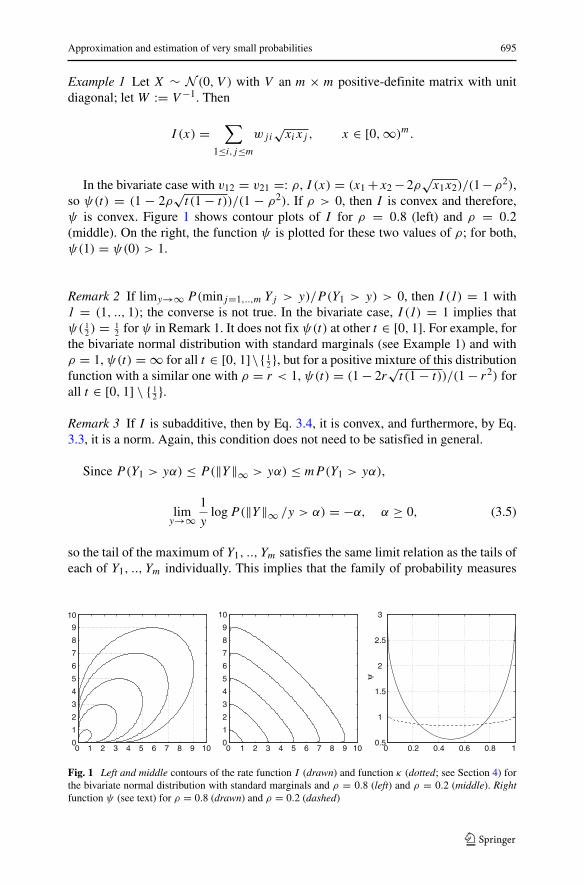
Example 1 Let X ∼ N (0, V ) with V an m × m positive-definite matrix with unitdiagonal; letW := V −1. Then

I (x) =∑

1≤i,j≤mwji

√xixj , x ∈ [0,∞)m.

In the bivariate case with v12 = v21 =: ρ, I (x) = (x1 +x2 −2ρ√x1x2)/(1−ρ2),

so ψ(t) = (1 − 2ρ√t (1 − t))/(1 − ρ2). If ρ > 0, then I is convex and therefore,

ψ is convex. Figure 1 shows contour plots of I for ρ = 0.8 (left) and ρ = 0.2(middle). On the right, the function ψ is plotted for these two values of ρ; for both,ψ(1) = ψ(0) > 1.

Remark 2 If limy→∞ P(minj=1,..,m Yj > y)/P (Y1 > y) > 0, then I (1) = 1 with1 = (1, .., 1); the converse is not true. In the bivariate case, I (1) = 1 implies thatψ( 1

2 ) = 12 for ψ in Remark 1. It does not fix ψ(t) at other t ∈ [0, 1]. For example, for

the bivariate normal distribution with standard marginals (see Example 1) and withρ = 1, ψ(t) = ∞ for all t ∈ [0, 1]\ { 1

2 }, but for a positive mixture of this distributionfunction with a similar one with ρ = r < 1, ψ(t) = (1 − 2r

√t (1 − t))/(1 − r2) for

all t ∈ [0, 1] \ { 12 }.

Remark 3 If I is subadditive, then by Eq. 3.4, it is convex, and furthermore, by Eq.3.3, it is a norm. Again, this condition does not need to be satisfied in general.

Since P(Y1 > yα) ≤ P(‖Y‖∞ > yα) ≤ mP(Y1 > yα),

limy→∞

1

ylogP(‖Y‖∞ /y > α) = −α, α ≥ 0, (3.5)

so the tail of the maximum of Y1, .., Ym satisfies the same limit relation as the tails ofeach of Y1, .., Ym individually. This implies that the family of probability measures

0 1 2 3 4 5 6 7 8 9 100

1

2

3

4

5

6

7

8

9

10

0 1 2 3 4 5 6 7 8 9 100

1

2

3

4

5

6

7

8

9

10

0 0.2 0.4 0.6 0.8 10.5

1

1.5

2

2.5

3

ψ

Fig. 1 Left and middle contours of the rate function I (drawn) and function κ (dotted; see Section 4) forthe bivariate normal distribution with standard marginals and ρ = 0.8 (left) and ρ = 0.2 (middle). Rightfunction ψ (see text) for ρ = 0.8 (drawn) and ρ = 0.2 (dashed)

696 C. de Valk

corresponding to the random variables {Y/y, y > 0} is exponentially tight (Demboand Zeitouni 1998): for every α < ∞, a compact Eα ⊂ R

m exists such that

lim supy→∞

1

ylogP(Y/y ∈ Ecα) < −α, (3.6)

which follows from Eq. 3.5 when taking Eα = {x ∈ Rm : ‖x‖∞ ≤ α + ε} for some

ε > 0. As a consequence,

Proposition 3 Let Y := (Y1, .., Ym) be a random vector with standard exponentialmarginals. If it satisfies (3.2), then it satisfies (3.1) for all Borel A ⊂ [0,∞)m withgood rate function I satisfying (3.4), I (0) = 0 and the marginal condition

infx∈Rm: xj>λ

I (x) = λ, λ ≥ 0, j = 1, .., m. (3.7)

Proof By Theorem 4.1.11 in Dembo and Zeitouni (1998), Eq. 3.2 implies the weakLDP, i.e., the lower bound in Eq. 3.1 holds for all BorelA, and the upper bound of Eq.3.1 holds for all compact A. Because of exponential tightness (3.6), this implies theLDP (3.1); see Lemma 1.2.18 in Dembo and Zeitouni (1998). Then Eq. 3.7 followsfrom Eq. 3.1 and the exponential marginals of Y .

Remark 4 Equation 3.3 is implied by (3.7).

For a continuity set A of I satisfying that inf I (A) = inf I (Ao), the bounds in(3.1) reduce to a limit:

limy→∞

1

ylogP(Y ∈ Ay) = − inf I (A). (3.8)

A sufficient condition for a set A to be a continuity set of I is that I is continuousand A ⊂ Ao. Homogeneity (3.4) of I allows us to relax this condition: withoutassuming continuity of I , A is a continuity set if inf I (A) = I (x) for some x ∈ Ao ∩∪λ>0(λA

o) (∪λ>0(λAo) is the smallest cone containing Ao). A bivariate example is

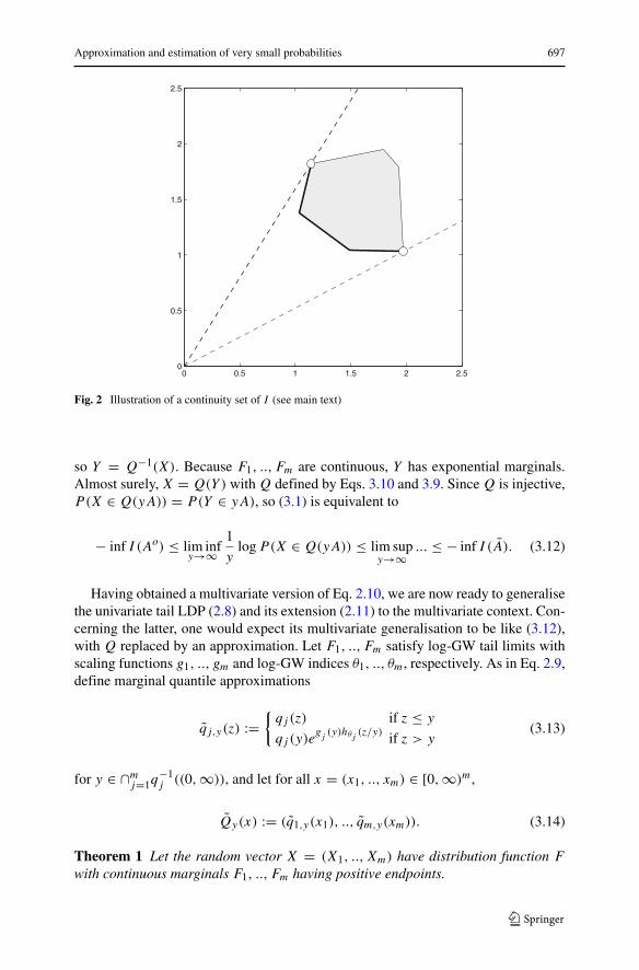
sketched in Fig. 2. Let Ao be the grey set; if I attains its infimum over A on the partof its boundary drawn as a fat line (excluding the points indicated by circles), then Ais a continuity set. In the remainder of this article, we will discuss continuity sets ofrate functions without considering the particular conditions which make them so.

It is straightforward to extend Proposition 3 to a random vector X with a dis-tribution function F having continuous marginals F1, .., Fm. As in Eq. 2.5, let fori = 1, .., m,

qi := F−1i (1 − e−Id) (3.9)

and for every x ∈ [0,∞)m,

Q(x) := (q1(x1), .., qm(xm)). (3.10)

Let Y := (Y1, .., Ym) with for j = 1, .., m,

Yj := − log(1 − Fj (Xj )), (3.11)

Approximation and estimation of very small probabilities 697

0 0.5 1 1.5 2 2.50

0.5

1

1.5

2

2.5

Fig. 2 Illustration of a continuity set of I (see main text)

so Y = Q−1(X). Because F1, .., Fm are continuous, Y has exponential marginals.Almost surely, X = Q(Y) withQ defined by Eqs. 3.10 and 3.9. SinceQ is injective,P(X ∈ Q(yA)) = P(Y ∈ yA), so (3.1) is equivalent to

− inf I (Ao) ≤ lim infy→∞

1

ylogP(X ∈ Q(yA)) ≤ lim sup

y→∞... ≤ − inf I (A). (3.12)

Having obtained a multivariate version of Eq. 2.10, we are now ready to generalisethe univariate tail LDP (2.8) and its extension (2.11) to the multivariate context. Con-cerning the latter, one would expect its multivariate generalisation to be like (3.12),with Q replaced by an approximation. Let F1, .., Fm satisfy log-GW tail limits withscaling functions g1, .., gm and log-GW indices θ1, .., θm, respectively. As in Eq. 2.9,define marginal quantile approximations

qj,y(z) :={qj (z) if z ≤ yqj (y)e

gj(y)hθj (z/y) if z > y

(3.13)

for y ∈ ∩mj=1q−1j ((0,∞)), and let for all x = (x1, .., xm) ∈ [0,∞)m,

Qy(x) := (q1,y(x1), .., qm,y(xm)). (3.14)

Theorem 1 Let the random vector X = (X1, .., Xm) have distribution function Fwith continuous marginals F1, .., Fm having positive endpoints.

698 C. de Valk

(a) If Y defined by Eq. 3.11 satisfies (3.2) and the marginals satisfy log-GW taillimits (2.6) with q = qj , g = gj and θ = θj for j = 1, .., m, then X satisfies

− inf I (Ao) ≤ lim infy→∞

1

ylogP(X ∈ Qy(yA)) ≤ lim sup

y→∞... ≤ − inf I (A) (3.15)

for every Borel set A ⊂ [0,∞)m, with Qy given by Eqs. 3.13 and 3.14, and I a goodrate function satisfying (3.4), (3.7) and I (0) = 0.

(b) If X satisfies (3.15) for every Borel set A ⊂ [0,∞)m with Qy given by Eqs.3.13 and 3.14 and with rate function I satisfying (3.7), then the marginals satisfylog-GW tail limits, and Y defined by Eq. 3.11 satisfies (3.1) with good rate functionI satisfying (3.4), (3.7) and I (0) = 0.

The proof can be found in Section 8.1.

Remark 5 This theorem justifies viewing (3.1) as representation of tail dependencewithin the context of the LDP (3.15), which also represents the marginal tails. Therelationship between the LDPs (3.15) and (3.1) is the large deviations analogue of asimilar relationship in classical extreme value theory; compare e.g. Resnick (1987),Propositions 5.10 and 5.15.

From the multivariate generalisation of Eq. 2.11, we can now also derive amultivariate version of Eq. 2.8, equivalent to the restriction of Eq. 3.15 to A ⊂[1,∞)m:

Corollary 1 Let θ := (θ1, .., θm) and Hθ(z) := (hθ1(z1), .., hθm(zm)) for all z ∈(0,∞)m. Then Eq. 3.15 implies for every Borel set D ∈ [0,∞)m:

− inf I (H−1θ (Do))

≤ lim infy→∞

1

ylogP

((logX1 − log q1(y)

g1(y), ..,

logXm − log qm(y)

gm(y)

)∈ D

)(3.16)

≤ lim supy→∞

... ≤ − inf I (H−1θ (D)).

Proof See Section 8.1.

Note that Eq. 3.16 only addresses events within (q1(y),∞) × .. × (qm(y),∞),which is “covered” by all marginal log-GW tail approximations simultaneously. Justas Eq. 2.8, it can be extended somewhat. However, the main interest of Eq. 3.16 is thatit shows the multivariate tail LDP explicitly as a pair of asymptotic bounds for theprobabilities of extreme events defined in terms of affinely normalised logarithms ofthe components of X. For applications in statistics, Eq. 3.15 should be more useful,as it applies also to events which are not simultaneously extreme in every componentof X.

Approximation and estimation of very small probabilities 699

4 A connection to residual tail dependence and related models

In this section, we digress from the main storyline to examine an interesting connec-tion between the theory of Section 3 and earlier work on residual tail dependence(RTD) or hidden regular variation, introduced in Ledford and Tawn (1996, 1997,1998) and studied in depth in Resnick (2002), amongst others. In the bivariate case,RTD offers a model of tail dependence within the classical domain of asymptoticindependence of component-wise maxima (e.g. de Haan and Ferreira (2006), Section7.6). For a random vector X on R

m with continuous marginals F1, ..., Fm, definingthe random vector V := (V1, .., Vm) with standard Pareto-distributed variables byEq. 1.4, one way to describe RTD is that for some positive function S on (0,∞)m,

limt→∞

P(Vj > txj , j = 1, .., m)

P (Vj > t, j = 1, .., m)=: S(x) > 0, x ∈ (0,∞)m. (4.1)

The limiting function S satisfies S(1) = 1, with 1 the vector in Rm with all its

components equal to 1. Furthermore, the denominator in Eq. 4.1 must be regularlyvarying, so S(λ1) = λ−1/η for all λ > 0 with η ∈ (0, 1] the residual dependenceindex, and by Eq. 4.1,

S(xλ) = λ−1/ηS(x), x ∈ (0,∞)m, λ > 0. (4.2)

Every regularly varying function f ∈ RVα can be represented as

f (y) = c(y)e

∫ yy0a(t)t−1dt

(4.3)

with c(y) → c0 > 0 and a(y) → α as y → ∞. A minor strengthening of regularvariation is that f satisfies the Von Mises condition (see e.g. Proposition 1.15 ofResnick (1987)), which means that c in Eq. 4.3 can be taken equal to a positivenumber c0; it implies that f is differentiable with derivative f ′(y) = a(y)f (y)/y.Note that whenever the LDP (3.1) holds for Y given by Eq. 3.11 and inf I (A) ∈(0,∞) for a Borel continuity set A of I , then the function (y �→ − logP(Y/y ∈ A))is in RV1. Therefore, within the context of the LDP (3.1), the statement that (y �→− logP(Y/y ∈ A)) satisfies the Von Mises condition makes sense as a smoothnesscondition. The following relates RTD to the tail LDP (3.1).

Proposition 4 (a) RTD (4.1) implies

limy→∞

1

ylogP(Y/y ∈ (λ,∞)m) = −λ/η, λ > 0, (4.4)

with η the residual dependence index of X.(b) If X satisfies the LDP (3.1) with the function (y �→ − logP(Y/y ∈ (1,∞)m))

satisfying the Von Mises condition, then Eq. 4.1 holds for x = λ1 for all λ > 0, withS satisfying S(1λ) = λ

−1/η and η = 1/I (1).

Proof Define Y∧ := minj∈{1,..,m} Yj , and let H∧ be the distribution function of Y∧ .By Eq. 4.1, the survival function 1 − H∧ ◦ log of the random variable exp Y∧ is

700 C. de Valk

regularly varying with index −1/η. Therefore, f := 1/(1 −H∧ ◦ log) ∈ RV{1/η}, soby the Potter bounds (Bingham et al. 1987), for every ε ∈ (0, 1/η),there is zε > 0 suchthat (1 − ε)(x/z)1/η−ε ≤ f (x)/f (z) ≤ (1 + ε)(x/z)1/η+ε for all z ≥ zε and x ≥ z.Taking logarithms and substituting eyλ for x gives limy→∞ y−1 log f (eyλ) → λ/η

for all λ > 0, so Eq. 4.4 follows. For (b), note that due to Eq. 3.4, the LDP (3.1)implies (4.4) with η = 1/I (1), so w(y) := − log(1 − H∧(y)) ∼ y/η as y → ∞.Therefore, sincew satisfies the Von Mises condition,w′(y) → 1/η and by averaging,w(y + r) − w(y) → r/η as y → ∞ for every r ∈ R. This is equivalent to Eq. 4.1for x = λ1 with S(1λ) = λ

−1/η for every λ > 0.

Proposition 4 shows that RTD implies a limited LDP-like condition and in turn, theLDP (3.1) with an additional smoothness condition implies an RTD-like condition.

Example 2 The bivariate normal X of Example 1 satisfies the conditions for Propo-sition 4(b) with I (1) = 2/(1 + ρ). Indeed, Eq. 4.1 holds for x = λ1 for all λ > 0,with S(1λ) = λ

−1/η and η = (1 +ρ)/2; see Example Class 2(1) in Ledford and Tawn(1996).

If limt→∞ t−1P(Vj > t, j = 1, .., m) = 0, then there is a discrepancy betweenthe “hidden” regularity of the survival function in (0,∞)m described by Eq. 4.1 andthe regularity of the marginals. In contrast, the LDP (3.1) provides a single consistentdescription of the multivariate tail which includes the marginal tails. Furthermore,the next theorem shows that under a smoothness assumption similar to the one inProposition 4(b), the LDP (3.1) implies a useful extension of RTD. Let for all a ∈Rm,

Aa := {x ∈ Rm : xj > aj , j = 1, .., m}. (4.5)

Theorem 2 (a) Assume that the LDP (3.1) applies. To any Borel setA ⊂ Rm which

is a continuity set of I with (y �→ − logP(Y/y ∈ A)) satisfying the Von Misescondition, the following limit relation applies:

limt→∞

P(Y ∈ A log(tλ))

P (Y ∈ A log t)= λ− inf I (A), λ > 0, (4.6)

with I satisfying (3.4), (3.7) and I (0) = 0. In particular, for every a ∈ [0,∞)msuch that the function (y �→ − logP(Yj > yaj , j ∈ 1, .., m) satisfies the VonMises condition,

limt→∞

P(Vj > (tλ)aj , j = 1, .., m)

P (Vj > taj , j = 1, .., m)

= λ− inf I (Aa), λ > 0. (4.7)

(b) Equation 4.6 with inf I (A) ∈ (0,∞) implies (3.8).

Proof ForA a continuity set of I , (3.1) implies (3.8), and (4.6) is obtained in the samemanner as in the proof of Proposition 4(b). In particular,Aa is a continuity set of I forevery a ∈ [0,∞)m. Therefore, substituting Aa for A in Eq. 4.6, we obtain (4.7). Thisproves (a). For (b), note that f := (t �→ 1/P (Y ∈ A log t)) ∈ RVinf I (A). Therefore,

Approximation and estimation of very small probabilities 701

just as in the proof of Proposition 4(a), limy→∞ y−1 log f (eyλ) → λ inf I (A) for allλ ≥ 1, which implies (3.8).

Combining (a) and (b) in Theorem 2, we see that under the Von Mises condition(for A a Borel continuity set of I ), the limit relation (4.6) for a probability ratio, andthe limit relation (3.8) for the normalised logarithm of a probability are equivalent.

In the special case of a = 1, Eq. 4.7 becomes equivalent to Eq. 4.1 with x = λ1and η = 1/I (1), so on the diagonal, Eq. 4.7 and RTD (4.1) agree; elsewhere, theydiffer. Defining a function κ by κ(a) := inf I (Aa) for every a ∈ [0,∞)m, Eq. 4.7becomes identical to an extension of RTD recently introduced in Wadsworth andTawn (2013). Wadsworth and Tawn (2013) proposed this assumption to close thepossible gap between (4.1) and the regularity of the marginal tails. It is curious thatthis condition, requiring the existence of separate limits of the survival function alongchosen paths, is derivable from the simple LDP (3.1).

The generalisation of Eq. 4.7 with inf I (Aa) replaced by κ(a) to the apparentlynew limit relation (4.6) is not trivial. Another generalisation, proposed in Wadsworthand Tawn (2013), is

limt→∞

P(Y ∈ B + a log(tλ))

P (Y ∈ B + a log t)= λ−κ(a), λ > 0, (4.8)

derived in Section 3.3 of Wadsworth and Tawn (2013) for the bivariate case under theassumption that κ is differentiable and a ∈ [0,∞)m \ {0} satisfies ∂κ(a)/∂aj > 0for j = 1, .., m. As noted in Wadsworth and Tawn (2013), a in Eq. 4.8 would have tobe chosen in an application. This would be no problem if the choice did not matter.However, the limiting behaviour of the probability of the event Y ∈ B+a log t as t →∞ is determined by a in Eq. 4.8; not by B. Therefore, for estimating probabilities ofextreme events, Eq. 4.6 seems more promising than the local limits (4.8) for chosena.

In Eq. 4.6, it is not κ , but the rate function I which determines the attenuationrate. For any a ∈ [0,∞)m, I (a) and κ(a) are identical only if I (a + x) ≥ I (a) forall x ∈ [0,∞)m. This condition is rather restrictive, as a rate function resembles adensity more than it resembles a survival function; see definition (3.2).

Example 3 As an illustration, let X be bivariate normal with correlation coefficientρ as in Example 1 (Section 3). By Example 1(a,b) in Table 1 of Wadsworth and Tawn(2013), κ(x) = I (x) if min(x1/x2, x2/x2) > ρ2 or if ρ < 0 and min(x1, x2) > 0,and κ(x) = max(x1, x2) for all other x ∈ [0,∞)2. The left and middle panels ofFig. 1 display contours of κ overlaying the contours of I for ρ = 0.8 and ρ = 0.2.For ρ = 0.2, contours of κ largely overlap with those of I ; for ρ = 0.8, there arewide zones where the contours of κ and I differ.

5 A simple estimator for very small probabilities

We are now going to apply the theory of Section 3 to the problem of estima-tion of probabilities of extreme events pn satisfying (1.1) from X(1), ..., X(n),

702 C. de Valk

with X(1), X(2), ... a sequence of iid copies of a random vector X in Rm with

distribution function F having continuous marginals F1, .., Fm. Denoting the under-lying probability space as (�,F,P), let Fn ⊂ F be the σ -algebra generated byX(1), ..., X(n).

Generalising (1.1) to τ2 > τ1 > 0, consider events of the form Bn := Q(A log n)with A ⊂ [0,∞)m and Q given by Eq. 3.10. Suppose that the tail LDP (3.1)applies. Then for every Borel set A ⊂ [0,∞)m which is a continuity set of Isatisfying that inf I (A) ∈ (0,∞), we have: − logP(X ∈ Bn) = − logP(Y ∈A log n) ∼ (log n) inf I (A) and − logP(Q(Y/�) ∈ Bn) = − logP(Y ∈ A� log n) ∼�(log n) inf I (A) for all � > 0, so

logP(X ∈ Bn) ∼ �−1 logP(Q(Y/�) ∈ Bn), � > 0. (5.1)

This suggests estimating the left-hand side of Eq. 5.1 by replacingQ on the right-hand side by an estimator Qn and Y by an estimator Yn, and then choosing � smallenough that P(Qn(Yn/�) ∈ Bn) can be estimated nonparametrically by counting.

Estimation of Q boils down to a univariate quantile estimation problem, so weproceed to examine this first. Assume that every marginal satisfies a log-GW taillimit (i.e., the univariate tail LDP, see Section 2). Let Xj,1:n ≤ ... ≤ Xj,n:n be the

marginal order statistics derived from the marginal sample X(1)j , ..., X(n)j . For some

intermediate sequence (kn) and for n large enough that Xj,n−kn+1:n > 0 for j =1, .., m, define the following estimator qj,n for qj (compare (3.13)):

qj,n(z) :={Xj,�n(1−e−z)�+1:n if z ∈ [0, yn]Xj,n−kn+1:n exp

(gj,nhθj,n

(z/yn))

if z > yn(5.2)

with

yn := log(n/kn). (5.3)

For z > yn, qj,n(z) follows a log-GW tail with θj,n and gj,n estimators for θj andgj in Eq. 3.13, respectively; for other z, the empirical quantile is used as estimator.The only assumption we make on the quantile estimator is that the probability-basedquantile estimation error νj,n, defined by

νj,n(z) := log(1 − Fj (qj,n(z)))log(1 − Fj (qj (z))) − 1 = q−1

j qj,n(z)

z− 1, z ≥ 0 (5.4)

satisfies for all � > 1 and j = 1, .., m that

limn→∞ sup

λ∈[1,�]

∣∣νj,n(ynλ)∣∣ = 0 a.s. (5.5)

Estimators θn,j and gn,j in Eq. 5.2 satisfying this requirement were considered inde Valk (2016). Let

Qn(x) := (q1,n(x1), ..., qm,n(xm)) (5.6)

Approximation and estimation of very small probabilities 703

for every x ∈ [0,∞)m. Define as estimator for Y (i)j := − log(1 − F(X(i)j )):Y(i)j,n := − log(1 − (R(i)j,n − 1

2 )/n) (5.7)

with R(i)j,n := ∑nl=1 1(X

(l)j ≤ X(i)j ) the marginal rank of X(i)j .

For every n-tuple of events Cn := (C(1)n , .., C(n)n ) satisfying C(i)n ∈ Fn for i =1, .., n, define the “empirical probability” pn(Cn) := ω �→ pn(Cn)(ω) on � by

pn(Cn)(ω) := n−1n∑i=1

1(ω ∈ C(i)n ). (5.8)

For some ξ > 0, determine a value of the analogue of � in Eq. 5.1 as

�+n (B) := sup{l > 0 : pn(Qn(Yn/ l) ∈ B) ≥ (kn/n)ξ }, (5.9)

with sup{∅} := 0 and with pn(Qn(Yn/ l) ∈ B) = n−1 ∑ni=1 1(Qn(Y

(i)n / l) ∈ B) in

accordance with (5.8).Let π denote the probability measure corresponding to F . Now consider the

following estimator for π(B) := P(X ∈ B):π In(B) := (kn/n)

ξ/�+n (B). (5.10)

If Bn,τ := Q(Aτ log n) is substituted for B, then under mild restrictions on A and(kn), this estimator converges in the large deviation sense for all τ > 0:

Theorem 3 Let X(1), X(2), ... be iid copies of a random vector X on Rm satisfying

the conditions of Theorem 1(a), including continuous marginals satisfying log-GWtail limits. For a sequence (kn) satisfying

0 ≤ c′ := lim infn→∞

log knlog n

≤ lim supn→∞

log knlog n

=: c < 1, (5.11)

consider the estimator (5.10) for P(X ∈ B), with the quantile estimator (5.2) sat-isfying (5.5) and with ξ ∈ (0, (1 − c′)−1). Then for Bn,τ := Q(Aτ log n), withA ⊂ [0,∞)m any Borel set which is a continuity set of I defined by Eqs. 3.2 and3.11 and satisfies inf I (A) ∈ (0,∞),

limn→∞ sup

τ∈[T −1,T ]

∣∣∣∣ log π In(Bn,τ )

logP(X ∈ Bn,τ ) − 1

∣∣∣∣ = 0 a.s. (5.12)

for every T > 1.

The proof can be found in Section 8.3.

Remark 6 By Eq. 3.12, as inf I (Ao) = inf I (A), P(X ∈ Bn,τ ) = n−τ inf I (A)(1+o(1))in Eq. 5.12, so the probability range (1.1) is covered by Theorem 3.

In practice, computing or approximating (5.9) may not be easy; for example, inengineering applications, it may involve running a complex numerical model for

704 C. de Valk

every datapoint. Therefore, it would be an advantage to replace �+n (B) in Eq. 5.10 byan arbitrary value in some suitable interval. Define for some ϑ ∈ (0, ξ ]

�−n (B) := sup{l > 0 : pn(Qn(Yn/ l) ∈ B) ≥ (kn/n)ϑ }. (5.13)

Then �−n (B) ≤ �+n (B). Let �n(B) be the result of an algorithm designed to satisfy

�n(B) ∈ [�−n (B), �+n (B)]; (5.14)

for the present analysis, it is sufficient to assume that �n(B) is a random variablesatisfying (5.14). Now consider the following generalisation of the estimator (5.10)for π(B) := P(X ∈ B):

π IIn (B) :=

(pn(Qn(Yn/�n(B)) ∈ B)

)1/�n(B). (5.15)

Theorem 4 For X(1), X(2), ..., (kn) and c′ as in Theorem 3, consider the estimator(5.15) for P(X ∈ B), with the quantile estimator (5.2) satisfying (5.5) and withξ ∈ (0, (1 − c′)−1) and ϑ ∈ (0, ξ ]. Then for Bn,τ as in Theorem 3,

limn→∞ sup

τ∈[T −1,T ]

∣∣∣∣ log π IIn (Bn,τ )

logP(X ∈ Bn,τ ) − 1

∣∣∣∣ = 0 a.s. (5.16)

for every T > 1.

The proof can be found in Section 8.2.The constraints on (kn), ξ and ϑ ensure that for some ε ∈ (0, 1

2 ),eventually,

nε < npn(Qn(Yn/�n(Bn,τ )) ∈ Bn,τ ) < n1−ε. This does not seem restrictive forapplications.

In practice, based on a few trial values of �n(B) which give “acceptable” numbersof npn(Qn(Yn/�n(B)) ∈ B), one could check the stability of π II

n (B) with respect tonpn(Qn(Yn/�n(B)) ∈ B).

6 Numerical examples

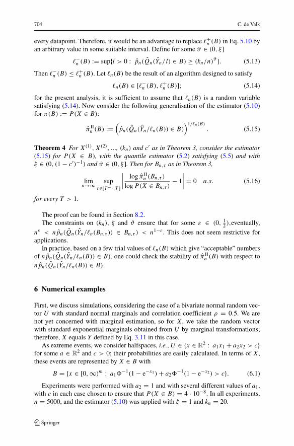
First, we discuss simulations, considering the case of a bivariate normal random vec-tor U with standard normal marginals and correlation coefficient ρ = 0.5. We arenot yet concerned with marginal estimation, so for X, we take the random vectorwith standard exponential marginals obtained from U by marginal transformations;therefore, X equals Y defined by Eq. 3.11 in this case.

As extreme events, we consider halfspaces, i.e., U ∈ {x ∈ R2 : a1x1 + a2x2 > c}

for some a ∈ R2 and c > 0; their probabilities are easily calculated. In terms of X,

these events are represented by X ∈ B with

B = {x ∈ [0,∞)m : a1�−1(1 − e−x1)+ a2�

−1(1 − e−x2) > c}. (6.1)

Experiments were performed with a2 = 1 and with several different values of a1,with c in each case chosen to ensure that P(X ∈ B) = 4 · 10−8. In all experiments,n = 5000, and the estimator (5.10) was applied with ξ = 1 and kn = 20.

Approximation and estimation of very small probabilities 705

0 5 10 15 20 25 300

5

10

15

20

25

30

0 5 10 15 20 25 300

5

10

15

20

25

30

0 5 10 15 20 25 300

5

10

15

20

25

30

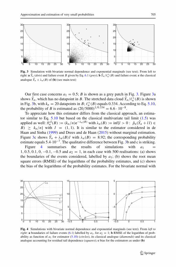
Fig. 3 Simulation with bivariate normal dependence and exponential marginals (see text). From left toright: a Yn (dots) and failure event B given by Eq. 6.1 (grey); b Yn/�+n (B) and failure event; c the classicalanalogue Yn + λn(B) of (b) (see main text)

Our first case concerns a1 = 0.5; B is shown as a grey patch in Fig. 3. Figure 3ashows Yn, which has no datapoint in B. The stretched data cloud Yn/�+n (B) is shownin Fig. 3b, with kn = 20 datapoints in B; �+n (B) equals 0.334. According to Eq. 5.10,the probability of B is estimated as (20/5000)1/0.334 = 6.6 · 10−8.

To appreciate how this estimator differs from the classical approach, an estima-tor similar to Eq. 5.10 but based on the classical multivariate tail limit (1.5) wasapplied as well: πcl

n (B) := (kn/n)e−λn(B) with λn(B) := inf{l > 0 : pn(Yn + l1) ∈B) ≥ kn/n} with 1 = (1, 1). It is similar to the estimator considered in deHaan and Sinha (1999) and Drees and de Haan (2015) without marginal estimation.Figure 3c shows Yn + λn(B)1 with λn(B) = 8.92; the corresponding probabilityestimate equals 5.4·10−7. The qualitative difference between Fig. 3b and c is striking.

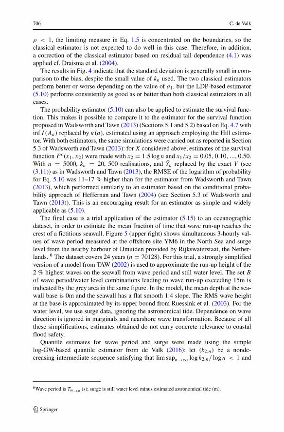
Figure 4 summarises the results of simulations with a1 =1, 0.5, 0.1, 0,−0.1,−0.5 and a2 = 1, in each case with 500 realisations: (a) showsthe boundaries of the events considered, labelled by a1; (b) shows the root meansquare errors (RMSE) of the logarithms of the probability estimates, and (c) showsthe bias of the logarithms of the probability estimates. For the bivariate normal with

0 5 10 15 20 25 300

5

10

15

20

25

1

0.5

0.1

0

−0.1

−0.5

−0.5 0 0.5 10

5

10

15

−0.5 0 0.5−10

−5

0

5

Fig. 4 Simulations with bivariate normal dependence and exponential marginals (see text). From left toright: a boundaries of failure events (6.1) labelled by a1, for a2 = 1; b RMSE of the logarithm of prob-ability as function of a1 for estimator (5.10) (circles), its classical analogue (diamonds) and its classicalanalogue accounting for residual tail dependence (squares); c bias for the estimators as under (b)

706 C. de Valk

ρ < 1, the limiting measure in Eq. 1.5 is concentrated on the boundaries, so theclassical estimator is not expected to do well in this case. Therefore, in addition,a correction of the classical estimator based on residual tail dependence (4.1) wasapplied cf. Draisma et al. (2004).

The results in Fig. 4 indicate that the standard deviation is generally small in com-parison to the bias, despite the small value of kn used. The two classical estimatorsperform better or worse depending on the value of a1, but the LDP-based estimator(5.10) performs consistently as good as or better than both classical estimators in allcases.

The probability estimator (5.10) can also be applied to estimate the survival func-tion. This makes it possible to compare it to the estimator for the survival functionproposed in Wadsworth and Tawn (2013) (Sections 5.1 and 5.2) based on Eq. 4.7 withinf I (Aa) replaced by κ(a), estimated using an approach employing the Hill estima-tor. With both estimators, the same simulations were carried out as reported in Section5.3 of Wadsworth and Tawn (2013): forX considered above, estimates of the survivalfunction Fc(x1, x2) were made with x2 = 1.5 log n and x1/x2 = 0.05, 0.10, ..., 0.50.With n = 5000, kn = 20, 500 realisations, and Yn replaced by the exact Y (see(3.11)) as in Wadsworth and Tawn (2013), the RMSE of the logarithm of probabilityfor Eq. 5.10 was 11–17 % higher than for the estimator from Wadsworth and Tawn(2013), which performed similarly to an estimator based on the conditional proba-bility approach of Heffernan and Tawn (2004) (see Section 5.3 of Wadsworth andTawn (2013)). This is an encouraging result for an estimator as simple and widelyapplicable as (5.10).

The final case is a trial application of the estimator (5.15) to an oceanographicdataset, in order to estimate the mean fraction of time that wave run-up reaches thecrest of a fictitious seawall. Figure 5 (upper right) shows simultaneous 3-hourly val-ues of wave period measured at the offshore site YM6 in the North Sea and surgelevel from the nearby harbour of IJmuiden provided by Rijkswaterstaat, the Nether-lands. 6 The dataset covers 24 years (n = 70128). For this trial, a strongly simplifiedversion of a model from TAW (2002) is used to approximate the run-up height of the2 % highest waves on the seawall from wave period and still water level. The set Bof wave period/water level combinations leading to wave run-up exceeding 15m isindicated by the grey area in the same figure. In the model, the mean depth at the sea-wall base is 0m and the seawall has a flat smooth 1:4 slope. The RMS wave heightat the base is approximated by its upper bound from Ruessink et al. (2003). For thewater level, we use surge data, ignoring the astronomical tide. Dependence on wavedirection is ignored in marginals and nearshore wave transformation. Because of allthese simplifications, estimates obtained do not carry concrete relevance to coastalflood safety.

Quantile estimates for wave period and surge were made using the simplelog-GW-based quantile estimator from de Valk (2016): let (k2,n) be a nonde-creasing intermediate sequence satisfying that lim supn→∞ log k2,n/ log n < 1 and

6Wave period is Tm−1,0 (s); surge is still water level minus estimated astronomical tide (m).

Approximation and estimation of very small probabilities 707

0 5 10 15 20 25 30

10−10

10−8

10−6

10−4

10−2

100

X1

PoE

−1 0 1 2 3 4 5

10−10

10−8

10−6

10−4

10−2

100

X2

PoE

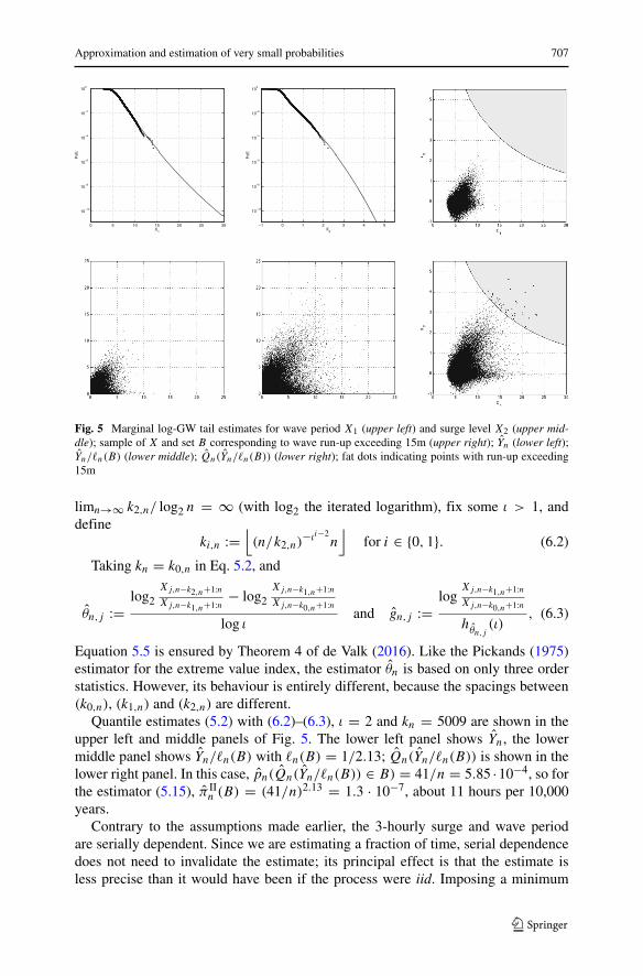
Fig. 5 Marginal log-GW tail estimates for wave period X1 (upper left) and surge level X2 (upper mid-dle); sample of X and set B corresponding to wave run-up exceeding 15m (upper right); Yn (lower left);Yn/�n(B) (lower middle); Qn(Yn/�n(B)) (lower right); fat dots indicating points with run-up exceeding15m

limn→∞ k2,n/ log2 n = ∞ (with log2 the iterated logarithm), fix some ι > 1, anddefine

ki,n :=⌊(n/k2,n)

−ιi−2n⌋

for i ∈ {0, 1}. (6.2)

Taking kn = k0,n in Eq. 5.2, and

θn,j :=log2

Xj,n−k2,n+1:nXj,n−k1,n+1:n − log2

Xj,n−k1,n+1:nXj,n−k0,n+1:n

log ιand gn,j :=

logXj,n−k1,n+1:nXj,n−k0,n+1:n

hθn,j(ι)

, (6.3)

Equation 5.5 is ensured by Theorem 4 of de Valk (2016). Like the Pickands (1975)estimator for the extreme value index, the estimator θn is based on only three orderstatistics. However, its behaviour is entirely different, because the spacings between(k0,n), (k1,n) and (k2,n) are different.

Quantile estimates (5.2) with (6.2)–(6.3), ι = 2 and kn = 5009 are shown in theupper left and middle panels of Fig. 5. The lower left panel shows Yn, the lowermiddle panel shows Yn/�n(B) with �n(B) = 1/2.13; Qn(Yn/�n(B)) is shown in thelower right panel. In this case, pn(Qn(Yn/�n(B)) ∈ B) = 41/n = 5.85 ·10−4, so forthe estimator (5.15), π II

n (B) = (41/n)2.13 = 1.3 · 10−7, about 11 hours per 10,000years.

Contrary to the assumptions made earlier, the 3-hourly surge and wave periodare serially dependent. Since we are estimating a fraction of time, serial dependencedoes not need to invalidate the estimate; its principal effect is that the estimate isless precise than it would have been if the process were iid. Imposing a minimum

708 C. de Valk

separation of 24 hours between storm events, the 41 datapoints moved into B in Fig.5 (lower right) represent 18 distinct events, giving a mean duration per event of 6.8hours. Using this value, the estimate π II

n (B) can be converted to an estimate of thefrequency of wave run-up exceeding 15m; its value is 1.7 · 10−4 per year. Evidently,this unconventional, but intuitively appealing variation of the peaks-over-thresholdapproach would need formal underpinning by a model of serial dependence in orderto be taken seriously.

7 Discussion

Like similar methods in the classical setting (e.g. de Haan and Sinha (1999), Dreesand de Haan (2015), Draisma et al. (2004)), the estimators (5.10) and (5.15) exploithomogeneity of a function describing tail dependence; in this case, homogeneity (3.4)of the rate function I . This offers the advantage that no explicit estimate of I isrequired. However, in certain situations, there may be good reasons to estimate I ,such as if for a given random vectorX, probabilities need to be estimated for multiplesets in a consistent and reproducible manner. Therefore, estimation of I remains atopic deserving elaboration.

The limitation of A to continuity sets of I in Theorems 3 and 4 is less restrictivethan it may seem, since the homogeneity of I makes continuity sets rather common,as noted in Section 3. The other conditions on A are weak.

To prove convergence of the estimators under such weak conditions, local unifor-mity in d of convergence in Eq. 8.5 is employed, which is derived from uniformityin d of convergence in (8.12). The latter also ensures local uniformity in λ of conver-gence in Eq. 8.5, and therefore local uniformity in τ of convergence of the estimatorsin Eqs. 5.12 and 5.16. In practice, this means that if such an estimator applied to agiven dataset produces a fair estimate of P(X ∈ B0) for some B0 ⊂ R

m, then itmay also be applied with confidence to the same dataset to estimate the probabilityof B1 ⊂ R

m such that P(X ∈ B1) ≥ P(X ∈ B0)τ for τ > 1 not too large, e.g.

τ = 2. If P(X ∈ B0) � 1, e.g. P(X ∈ B0) = 0.01, this amounts to extrapolationover several additional orders of magnitude in probability. How far one can extrapo-late in practice will depend on the rates of convergence to the marginal log-GW taillimits and in Eq. 3.1, which will differ from case to case.

Convergence of log-probability ratios as in Eqs. 5.12 and 5.16 is typical for theprobability range (1.1). A stronger notion of convergence might be desirable, butwould require restrictive additional assumptions which would be hard to justify inapplications. Rather, it is recommended to diagnose bias in estimates and take thisinto account in estimates of uncertainty. For this reason, modelling of bias and rateof convergence deserves further study.

Deriving asymptotic error distributions will require additional assumptionsbeyond those for Theorems 3 and 4 and methods quite different from those employedin the present article. Because it is complex (see e.g. Drees and de Haan (2015) for acomparable problem), this important topic needs to be left for a follow-up study as well.

The theory is readily extended from events involving a high value of at least oneof the variables to events extreme “in any direction”, by replacing the exponential

Approximation and estimation of very small probabilities 709

distribution as standard marginal by the Laplace distribution cf. Keef et al. (2013).Other choices of standard marginal are also possible, with minor adaptations to theoryand estimator.

Furthermore, the main results of this article can be generalised straightforwardlyfrom a random vector in R

m to a random element of Cb(K), the continuous func-tions on a compact metric space K . Classical multivariate extreme value theory andestimation have been generalised to this setting earlier; see e.g. de Haan and Lin(2001), Part III of de Haan and Ferreira (2006), Einmahl and Lin (2006) and Fer-reira and de Haan (2014). For the theory presented here, the main difference betweenthe R

m setting and the Cb(K) setting is that in the latter, exponential tightness of{P(Y/y ∈ ·), y > 0} no longer follows from the exponential marginals; it is anindependent assumption. In loose terms, it entails that all but an exponentially smallprobability mass is concentrated on an equicontinuous set of functions in Cb(K) (seee.g. Dembo and Zeitouni (1998)).

8 Proofs and lemmas

8.1 Proof of Theorem 1 and Corollary 1

Convergence in Eq. 2.6 is locally uniform in λ (e.g. de Haan and Ferreira (2006),B.1.4 and B.2.9), so for all � > 1,

limy→∞ sup

λ∈[�−1,�]max

j=1,..,m

∣∣∣∣h−1θj

(log qj (yλ)− log qj (y)

gj (y)

)− λ

∣∣∣∣ = 0. (8.1)

For every y > 0, Qy is injective, so we can define the random vector

Yy := Q−1y (X) = Q−1

y Q(Y ) a.s. (8.2)

with Y defined by Eq. 3.11. By Eq. 8.1, there exists almost surely for every � > 1and δ > 0 some y�,δ > 0 such that for all y ≥ y�,δ , ‖Yy − Y‖∞ > δy implies‖Y‖∞ > �y. Therefore, by Eq. 3.5, since � > 1 is arbitrary, for all δ > 0,

limy→∞

1

ylogP(‖Yy − Y‖∞ > δy) = −∞. (8.3)

By Proposition 3, the distribution functions of {Y/y, y > 0} satisfy the LDP (3.1)with good rate function I , so Eq. 8.3 implies the same for the distribution functionsof {Yy/y, y > 0}; see Theorem 4.2.13 of Dembo and Zeitouni (1998). Therefore,Eq. 3.15 follows from (8.2). To prove (b), note that by Eqs. 3.15 and 3.7,

limy→∞

1

ylog

(1 − Fj

(qj (y)e

gj (y)hθj (λ)))

= −λ

for all λ ≥ 1 and j = 1, .., m, so Eq. 2.6 holds with q = qj , g = gj and θ = θjfor j = 1, .., m. As in the proof of (a), this implies (8.3). Moreover, Eq. 3.7 implies(3.3), so I is a good rate function. An application of Theorem 4.2.13 of Dembo andZeitouni (1998) completes the proof of the theorem.

710 C. de Valk

For the Corollary, note that for A ⊂ [1,∞)m, P(X ∈ Qy(yA)) in Eq. 3.15 isequal to

P

((logX1 − log q1(y)

g1(y), ..,

logXm − log qm(y)

gm(y)

)∈ Hθ(A)

)

by Eq. 3.13. Therefore, by the contraction principle (see Theorem 4.2.1 in Demboand Zeitouni (1998)), Eq. 3.16 follows from (3.15).

8.2 Proof of Theorem 4

For convenience, the following shorthand notation will be used:

μn,l(A) := pn(Qn(Yn/ l) ∈ Q(ynA)), (8.4)

and ln(A) := �n(Q(ynA)), l+n (A) := �+n (Q(ynA)), l−n (A) := �−n (Q(ynA)).By Proposition 3, Y defined by Eq. 3.11 satisfies the LDP (3.1) with good rate

function I . Noting that ξ ∈ (0, (1 − c′)−1) with c′ as in Eq. 5.11, take any � ∈(ξ/ inf I (A), (1 − c′)−1/ inf I (A)). Fixing an arbitrary� > 1, then by Lemma 4, forevery δ ∈ (0,�) (see (8.4)),

limn→∞ sup

λ∈[�−1,�], d∈[δ,�]

∣∣∣y−1n log μn,d/λ(Aλ)+ d inf I (A)

∣∣∣ = 0 a.s. (8.5)

and

lim supn→∞

supλ∈[�−1,�], d>�

y−1n log μn,d/λ(Aλ) ≤ −� inf I (A) < −ζ a.s. (8.6)

Choosing δ < ϑ/ inf I (A), since � > ξ/ inf I (A), we observe that

d inf I (A)

{ ≤ ξ if d ∈ [δ, ξ/ inf I (A)] ⊂ [δ,�]> ξ if d ∈ (ξ/ inf I (A),�] ⊂ [δ,�]

in Eq. 8.5. Therefore, with Eq. 8.6, using Eq. 5.9,

limn→∞ sup

λ∈[�−1,�]

∣∣λl+n (Aλ)− ξ/ inf I (A)∣∣ = 0 a.s. (8.7)

and similarly, using Eq. 5.13, we find that

limn→∞ sup

λ∈[�−1,�]

∣∣λl−n (Aλ)− ϑ/ inf I (A)∣∣ = 0 a.s. (8.8)

By Eqs. 8.7, 8.8, 5.14 and 8.5,

limn→∞ sup

λ∈[�−1,�]

∣∣∣y−1n l

−1n (Aλ) log μn,ln(Aλ)(Aλ)+ λ inf I (A)

∣∣∣ = 0 a.s. (8.9)

or equivalently, by Eq. 5.15,

limn→∞ sup

λ∈[�−1,�]

∣∣∣y−1n log π II

n (Q(ynAλ))+ λ inf I (A)∣∣∣ = 0 a.s. (8.10)

Approximation and estimation of very small probabilities 711

Since Eq. 3.12 holds with inf I (Ao) = inf I (A) and inf I (A) > 0, by Eqs. 3.4 and8.10,

limn→∞ sup

λ∈[�−1,�]

∣∣∣∣ log π IIn (Q(ynAλ))

logP(X ∈ Q(ynAλ)) − 1

∣∣∣∣ = 0 a.s.,

and Eq. 5.16 follows from Eq. 5.11, since � > 1 is arbitrary.

8.3 Proof of Theorem 3

Following the proof of Theorem 4 in Section 8.2, Eqs. 8.7 and 5.10 yield

limn→∞ sup

λ∈[�−1,�]

∣∣∣y−1n log π I

n(Q(ynAλ))+ λ inf I (A)∣∣∣ = 0,

and the result Eq. 5.12 follows as in the proof of Theorem 4.

8.4 Lemmas

Lemma 1 Let Y be a random vector in [0,∞)m with standard exponential marginalssatisfying the LDP (3.1) with good rate function I , and Y (1), Y (2), ... a sequence ofiid copies of Y . Let the Borel set A ⊂ [0,∞)m be a continuity set of I satisfyinginf I (A) ∈ (0,∞). If (yn > 0) and � > 0 satisfy limn→∞ yn = ∞ and

� < lim infn→∞

log n

yn inf I (A)< ∞, (8.11)

then with pn defined by Eq. 5.8, for all δ ∈ (0,Δ),limn→∞ sup

d∈[δ,�]

∣∣∣y−1n log pn(Y ∈ dAyn)+ d inf I (A)

∣∣∣ → 0 a.s., (8.12)

andlim supn→∞

supd>�

y−1n log pn(Y ∈ dAyn) ≤ −� inf I (A) a.s. (8.13)

Proof Let A := ∪λ≥1(λA); by Eq. 3.4, A is a continuity set of I satisfyinginf I (A) = inf I (A) < ∞. Define the random variable

v := inf{w > 0 : Yw ∈ A} (8.14)

with inf{∅} := ∞, and let G be its distribution function. Since ∪λ≥1(Aλ) ⊂ A,Y ∈ Aoz ⇒ v ≤ z−1 ⇒ Y ∈ Az for every z > 0, so by Eqs. 3.1 and 3.4, for allw > 0,

limy→∞ y

−1 logG(w/y) = −w−1 inf I (A). (8.15)

Therefore, since inf I (A) ∈ (0,∞), − logG(1/Id) ∈ RV{1}, so by Bingham et al.(1987) (Theorem 1.5.2) and Eq. 8.15 again, for every a > 0,

limy→∞ sup

w≥a

∣∣∣y−1 logG(w/y)+ w−1 inf I (A)∣∣∣ = 0. (8.16)

By Eq. 8.15, there is for every ε > 0 an nε ∈ N such that for all n ≥ nε,nG(a/yn) ≥ elog n−(ε+a−1 inf I (A))yn . (8.17)

712 C. de Valk

Taking a = 1/�, then by Eq. 8.11, ε > 0 can be chosen small enough that theexponent in Eq. 8.17 eventually exceeds ε log n. Therefore,

limn→∞ nG(a/yn)/ log n = ∞. (8.18)

WithG−1 the left-continuous inverse ofG, almost surely v(i) = G−1(U (i)) for alli ∈ N, with U (1),U (2), ... independent and uniformly distributed on (0, 1), so almostsurely (see def. (5.8)), pn(v ≤ w/yn) = pn(U ≤ G(w/yn)) for all n ∈ N and allw ≥ a. Therefore, by Wellner (1978) (Corollary 1) and (8.18),

limn→∞ sup

w≥a∣∣log pn(v ≤ w/yn)− logG(w/yn)

∣∣ = 0 a.s., (8.19)

and since v ≤ w/yn ⇒ Y ∈ Ayn/(wl)⇒ v ≤ wl/yn for all l > 1 and w > 0, usingEqs. 8.16 and 3.4, as a = 1/�,

limn→∞ sup

d∈(0,�]

∣∣∣y−1n log pn(Y ∈ dAyn)+ d inf I (A)

∣∣∣ = 0 a.s. (8.20)

Therefore, as A ⊂ A and inf I (A) = inf I (A),

lim supn→∞

supd∈(0,�]

y−1n log pn(Y ∈ dAyn)+ d inf I (A) ≤ 0 a.s. (8.21)

A is a continuity set of I and I satisfies (3.4), so there is for every ε > 0 apoint xε ∈ Ao such that I (xε) < inf I (A) + ε. Let ε > 0 and η > 1 be such that�η(inf I (A)+ ε) < lim infn→∞ y−1

n log n (see (8.11)). Then for η sufficiently closeto 1, an open set B ⊂ [0,∞)m can be constructed such that

∪λ≥1(λB) ⊂ B, xε ∈ B \ (Bη) ⊂ Ao, and

inf I (Bo) = inf I (B) ∈ (inf I (A), I (xε)] (8.22)as follows. The first two requirements on B are satisfied by B′ = ∪λ≥1(λU) forsome sufficiently small neighbourhood U ⊂ Ao of xε, with η > 1 close enough to1. If B′ is a continuity set of I , then set B = B′. Else, consider the function f :[0,∞)m×[0, 1] → [0,∞)m defined by f (y, a) := ay+ (1−a)(‖y‖∞ / ‖xε‖∞)xε.It satisfies f (B′, 1) = B′, f (B′, 0) = B′ ∩ ∪λ>0(λxε), and f (B′, a) ⊂ f (B′, a′)if a ≤ a′. Therefore, a �→ inf I (f (B′, a)) is non-increasing, so with α any of itscontinuity points in (0, 1), B = f (B′, α) is a continuity set of I and satisfies (8.22).By Eq. 8.22,

pn(Y ∈ dAyn) ≥ pn(Y ∈ dByn)− pn(Y ∈ dηByn)= pn(Y ∈ dByn)(1 − elog pn(Y∈dηByn)−log pn(Y∈dByn)), (8.23)

and furthermore, Eq. 8.20 continues to hold after substituting B or Bη for A. There-fore, by Eq. 3.4, for every δ ∈ (0,Δ) almost surely, the right-hand side of Eq. 8.23 ispn(Y ∈ dByn)(1 + o(1)) uniformly in d ∈ [δ,�] and furthermore, using Eq. 8.22,

lim infn→∞ inf

d∈[δ,�] y−1n log pn(Y ∈ dAyn)+ dI (xε) ≥ 0 a.s. (8.24)

Now Eq. 8.12 follows from Eqs. 8.21 and 8.24, because I (xε) < inf I (A) + ε, andε > 0 can be chosen arbitrarily close to 0. Finally, by Eq. 8.20, as ∪λ≥1(Aλ) ⊂ A,

lim supn→∞

supd>�

y−1n log pn(Y ∈ dAyn) ≤ −� inf I (A) a.s., (8.25)

Approximation and estimation of very small probabilities 713

and because A ⊂ A and inf I (A) = inf I (A), (8.13) follows.

Lemma 2 Let Y be a random vector on [0,∞)m with standard exponentialmarginals and Y (1), Y (2), ... a sequence of iid copies of Y . Define

Y (i)n := (Y(i)1,n, .., Y

(i)m,n)

for i = 1, .., n, with

Y(i)j,n := − log(1 − (R(i)j,n − 1

2 )/n) (8.26)

and

R(i)j,n :=

n∑l=1

1(Y (l)j ≤ Y (i)j ).

For (yn > 0) satisfying lim infn→∞ yn/ log n > 0,

supε>0

lim supn→∞

y−1n log pn(‖Yn − Y‖∞ > ynε) = −∞ a.s. (8.27)

Proof Since pn(‖Yn − Y‖∞ > ynε) ≤ ∑mj=1 pn(|Yj,n − Yj | > ynε), it is sufficient

to prove (8.27) for the univariate case.Let U (i) := exp(−Y (i)), and let Γn and Γ −1

n denote the empirical distributionfunction and the empirical quantile function of U (1), ..,U (n), which are independentand uniformly distributed in (0, 1). By Theorem 2 of Shorack and Wellner (1978), assupt∈[0,1] t−1Γn(t) = supt∈[1/n,1] t/Γ −1

n (t),

lim supn→∞

supt∈[1/n,1]

log(t/Γ −1n (t))/ log2 n = 1 a.s. (8.28)

Similarly, as supt∈[U1:n,1] t/Γn(t) = 1 ∨ supt∈[1/n,1] t−1Γ −1n (t), by Theorem 3 of

Shorack and Wellner (1978),

lim supn→∞

supt∈[1/n,1]

t−1Γ −1n (t)/ log2 n = 1 a.s.

solim infn→∞ inf

t∈[1/n,1] log(t/Γ −1n (t))/ log2 n = 0 a.s. (8.29)

Since Yn−i+1:n = − logΓ −1n (i/n), Yn−i+1:n = − log((i − 1

2 )/n), andyn/ log2 n → ∞, Eqs. 8.28 and 8.29 imply

maxi=1,..,n

|Yn−i+1:n − Yn−i+1:n|/yn → 0 a.s. (8.30)

As a consequence, there is almost surely for every ε > 0 an nε ∈ N such that for alln ≥ nε, pn(|Y − Yn| > ynε) = 0 and therefore y−1

n log pn(|Y − Yn| > ynε) = −∞,implying the univariate case of Eq. 8.27.

Lemma 3 Let X be a random vector on Rm having continuous marginals satisfying

log-GW tail limits, and let X(1), X(2), ... be a sequence of iid copies of X. With Q,Qn and Yn defined by Eqs. 3.10, 5.6 and 5.7, let (kn) satisfy (5.11) and qj,n defined

714 C. de Valk

by Eq. 5.2 satisfy (5.5) for j = 1, .., m, with yn defined by Eq. 5.3. Then for everyδ > 0 and ε > 0,

limn→∞ sup

l≥δy−1n log pn

(∥∥∥Q−1Qn(Ynl−1)− Ynl−1

∥∥∥∞ > ynε)

= −∞ a.s. (8.31)

Proof Fix ε > 0 and δ > 0. As in Lemma 2, we only need to prove (8.31) for theunivariate case, so we proceed with this. Note that Eq. 8.31 holds if an nδ,ε ∈ N

exists such that (suppressing the labels of vector components in the univariate case)

supl≥δ

maxj=1,..,n

|q−1qn(Yj :nl−1)− Yj :nl−1| ≤ ynε for all n ≥ nδ,ε. (8.32)

Fixing � > max(1, δ−1)/(1 − c) ≥ max(1, δ−1) lim supn→∞ log(2n)/yn with cas in Eqs. 5.11, 8.32 holds if

supz∈[0,yn�]

|q−1qn(z)− z| ≤ ynε for all n ≥ nδ,ε. (8.33)

Such an nδ,ε ∈ N exists if νn defined by Eq. 5.4 satisfies

supz∈[yn,yn�]

|νn(z)| → 0 (8.34)

and also,

supz∈[0,yn]

|q−1qn(z)− z|/yn = supt∈[e−yn ,1]

∣∣∣log(t/Γ −1n (t))

∣∣∣ /yn → 0, (8.35)

with U (1), ..,U (n) as in the proof of Lemma 2 (note that for all z ∈ [0, yn], q−1qn(z)

= q−1(X�n(1−e−z)�+1:n) = Y�n(1−e−z)�+1:n= − logΓ −1n (e−z)). As in the proof of

Lemma 2, Eqs. 8.28 and 8.29 hold. Therefore, since the upper bound in Eq. 5.11implies that lim infn→∞ yn/ log n > 0, Eq. 8.35 holds almost surely. Furthermore,by Eq. 5.5, (8.34) holds almost surely. This proves the univariate case.

Lemma 4 Let the random vector X on Rm have continuous marginals satisfying log-GW tail limits and let Y defined by Eq. 3.11 satisfy the LDP (3.1) with good ratefunction I . Let X(1), X(2), ... be a sequence of iid copies of X. Let (kn) satisfy (5.11)and let the quantile estimator qj,n given by Eq. 5.2 satisfy (5.5). Let the Borel setA ⊂ [0,∞)m be a continuity set of I satisfying inf I (A) ∈ (0,∞). Then μ definedby Eq. 8.4 satisfies for every � > 1 and every

� ∈(

0,1

(1 − c′) inf I (A)

)(8.36)

and δ ∈ (0,�):limn→∞ sup

λ∈[�−1,�], d∈[δ,�]

∣∣∣y−1n log μn,d/λ(Aλ)+ d inf I (A)

∣∣∣ = 0 a.s. (8.37)

and

lim supn→∞

supλ∈[�−1,�], d>�

y−1n log μn,d/λ(Aλ) ≤ −� inf I (A) a.s. (8.38)

Approximation and estimation of very small probabilities 715

Proof With {prop} denoting the subset of � satisfying the proposition prop,consider for positive a and b

C(i)a,b,n := {supl≥a

∥∥∥Q−1Qn(Y(i)n l

−1)− Y (i)l−1∥∥∥∞ > ynb}, i = 1, .., n, (8.39)

which are elements of Fn. Furthermore, following (5.8), we can define the empiricalprobability pn(Ca,b,n) := n−1 i∈{1,..,n}1(C(i)a,b,n). Combining Lemmas 2 and 3, weobtain

limn→∞ y

−1n log pn(Ca,b,n) = −∞ a.s. for all a, b > 0. (8.40)

For every S ⊂ Rm and ι > 0, let Sι := {x ∈ R

m : infx′∈S∥∥x − x′∥∥∞ ≤ ι}

(closed) and S−ι := {x ∈ Rm : infx′∈Sc

∥∥x − x′∥∥∞ > ι} (open). Set S0 := S. SinceI is a good rate function, Lemma 4.1.6 of Dembo and Zeitouni (1998) implies

limι↓0

inf I (Aι) = inf I (A) = inf I (Ao) = inf I (∪ι>0A−ι) = lim

ι↓0inf I (A−ι), (8.41)

so the non increasing function ι �→ inf I (Aι) is continuous in (−ι0, ι0) for someι0 > 0, and therefore, Aι is a continuity set of I for every ι ∈ (−ι0, ι0). Moreover, byEq. 8.36, there exist ε > 0 and ι1 ∈ (0, ι0) such that for all ι ∈ [0, ι1], inf I (A−ι) ≤inf I (A)+Δ−1ε < Δ−1(1 − c′)−1. Therefore, for

E(i)d,ι,n := {Y (i) ∈ dynAι} ∈ Fn, i = 1, .., n, (8.42)

Lemma 1 implies for � satisfying (8.36) and every δ ∈ (0,�) and ι ∈ [−ι1, ι1] that

limn→∞ sup

d∈[δ,�]

∣∣∣y−1n log pn(Ed,ι,n)+ d inf I (Aι)

∣∣∣ = 0 a.s., (8.43)

and therefore, as Δ inf I (A−ι1) < (1 − c′)−1,

infι∈[0,ι1]

lim infn→∞ inf

d∈[δ,�] y−1n log pn(Ed,−ι,n) ≥ −(1 − c′)−1 a.s. (8.44)

LetD(i)λ,d,n := {Qn(Y (i)n λ/d) ∈ Q(ynAλ)} ∈ Fn, i = 1, .., n. (8.45)

By Eqs. 8.42, 8.39 and 8.45, we have for all d ≥ δ, ι > 0 and λ ∈ [�−1,�] thatE(i)d,−ι,n ∩ (C(i)d/λ,ιλ,n)c ⊂ D

(i)λ,d,n, so pn(Dλ,d,n) ≥ pn(Ed,−ι,n) − pn(Cδ/�,ι/�,n).

Therefore, for all ι ∈ (0, ι1],lim infn→∞ inf

d∈[δ,�], λ∈[�−1,�]y−1n log pn(Dλ,d,n)− y−1

n log pn(Ed,−ι,n)

≥ lim infn→∞ y−1

n log(

1 − elog pn(Cδ/�,ι/�,n)−infd∈[δ,�] log pn(Ed,−ι,n))

≥ 0 a.s., (8.46)

the last inequality following from Eqs. 8.40 and 8.44. Therefore, by Eqs. 8.43 and8.41,

lim infn→∞ inf

d∈[δ,�], λ∈[�−1,�]y−1n log pn(Dλ,d,n)+ d inf I (A) ≥ 0 a.s. (8.47)

Furthermore, for all d ≥ δ, ι > 0 and λ ∈ [�−1,�], we have D(i)λ,d,n ∩(C(i)δ/�,ι/�,n)

c ⊂ E(i)d,ι,n, so D(i)λ,d,n ⊂ E

(i)d,ι,n ∪ C(i)δ/�,ι/�,n and therefore,

pn(Dλ,d,n) ≤ 2 max(pn(Cδ/�,ι/�,n), pn(Ed,ι,n)). (8.48)

716 C. de Valk

Therefore, by Eqs. 8.40, 8.43 and 8.41,

lim supn→∞

supd∈[δ,�], λ∈[�−1,�]

y−1n log pn(Dλ,d,n)+ d inf I (A) ≤ 0 a.s., (8.49)

so with Eqs. 8.47 and 8.4, Eq. 8.37 is obtained. By Lemma 1, with ι0 as above,

lim supn→∞

supd>�

y−1n log pn(Ed,ι,n) ≤ −� inf I (Aι) a.s. (8.50)

for all ι ∈ [0, ι0). Now Eq. 8.38 follows from Eq. 8.48 using Eqs. 8.40, 8.50 and8.41.

Acknowledgments The author wants to thank the Associate Editor, two Referees, John Einmahl andLaurens de Haan for their valuable comments and advice, which made the manuscript much better. Thesupport of Rijkswaterstaat by making the oceanographic data available is gratefully acknowledged.

Open Access This article is distributed under the terms of the Creative Commons Attribution 4.0International License (http://creativecommons.org/licenses/by/4.0/), which permits unrestricted use, dis-tribution, and reproduction in any medium, provided you give appropriate credit to the original author(s)and the source, provide a link to the Creative Commons license, and indicate if changes were made.

Compliance with Ethical Standards

Conflict of interests The author declares that he has no conflict of interest.

References

Bingham, N.H., Goldie, C.M., Teugels, J.L.: Regular variation. Cam. Univ. Press (1987)Broniatowski, M.: On the estimation of the Weibull tail coefficient. J. Stat. Plan. Inference 35, 349–366

(1993)Bruun, J.T., Tawn, J.A.: Comparison of approaches for estimating the probability of coastal flooding. J.

Roy. Statist. Soc. Ser. C 47, 405–423 (1998)Coles, S.G., Tawn, J.A.: Modelling extreme multivariate events. J. Roy. Statist. Soc. Ser. B 53, 377–392

(1991)Coles, S.G., Tawn, J.A.: Statistical methods for multivariate extremes: an application to structural design.

J. Roy. Statist. Soc. Ser. C 43(1), 1–48 (1994)Dembo, A., Zeitouni, O.: Large deviations techniques and applications. Springer, New York (1998)Draisma, G., Drees, H., Ferreira, A., de Haan, L.: Bivariate tail estimation: dependence in asymptotic

independence. Bernoulli 10, 251–280 (2004)Drees, H., de Haan, L.: Estimating failure probabilities. Bernoulli 21(2), 957–1001 (2015)Einmahl, J.H.J., Lin, T.: Asymptotic normality of extreme value estimators on C[0, 1]. Ann. Statist. 34,

469–492 (2006)Embrechts, P., Puccetti, G.: Aggregating risk across matrix structured loss data: the case of operational

risk. J. Oper. Risk 3(2), 29–44 (2007)Ferreira, A., de Haan, L.: The generalised Pareto process; with a view towards application and simulation.

Bernoulli 20(4), 171701737 (2014)de Haan, L., Sinha, A.K.: Estimating the probability of a rare event. Ann. Stat. 27(2), 732–759 (1999)de Haan, L., Lin, T.: On convergence toward an extreme value distribution in C[0, 1]. Ann. Probab. 29(1),

467–483 (2001)de Haan, L., Ferreira, A.: Extreme value theory - An introduction. Springer (2006)Hall, P.: On some simple estimates of an exponent of regular variation. J. Roy. Statist. Soc. Ser. B 44(1),

37–42 (1982)

Approximation and estimation of very small probabilities 717

Heffernan, J.E., Tawn, J.A.: A conditional approach for multivariate extreme values. J.R. Stat. Soc. Ser. B66, 497–546 (2004)

Heffernan, J.E., Resnick, S.I.: Hidden regular variation and the rank transform. Adv. Appl. Prob. 37(2),393–414 (2005)

Heffernan, J.E., Resnick, S.I.: Limit laws for random vectors with an extreme component. Ann. Appl.Probab. 17(2), 537–571 (2007)

ISO: Petroleum and natural gas industries - Specific requirements for offshore structures Part 1. ISO/FDIS,19901–1:2005(E) (2005)

Joe, H., Smith, R.L., Weissman, I.: Bivariate threshold methods for extremes. J. Roy. Statist. Soc. Ser. B54, 171–183 (1992)

Keef, C., Papastathopoulos, I., Tawn, J.S.: Estimation of the conditional distribution of a multivariatevariable given that one of its components is large: additional constraints for the Heffernan and Tawnmodel. J. Multivariate Anal. 115, 396–404 (2013)

Kluppelberg, C.: On the asymptotic normality of parameter estimates for heavy Weibull-like tails. Preprint(1991)

Ledford, A.W., Tawn, J.A.: Statistics for near independence in multivariate extreme values. Biometrika83(1), 169–187 (1996)

Ledford, A.W., Tawn, J.A.: Modelling dependence within joint tail regions. J. Roy. Statist. Soc. Ser. B 59,475–499 (1997)

Ledford, A.W., Tawn, J.A.: Concomitant tail behaviour for extremes. Adv. Appl. Prob. 30, 179–215 (1998)Peng, L.: Estimation of the coefficient of tail dependence in bivariate extremes. Stat. Probab. Lett. 43,

399–409 (1999)Pickands, J.: Statistical inference using extreme order statistics. Ann. Stat. 3, 119–131 (1975)Pickands, J.: Multivariate extreme value distributions. Bulletin of the International Statistical Institute:

Proceedings of the 43rd Session (Buenos Aires), 859–878 (1981)Resnick, S.I.: Extreme values, regular variation, and point processes. Springer (1987)Resnick, S.I.: Hidden regular variation, second order regular variation and asymptotic independence.

Extremes 5, 303–336 (2002)Ruessink, B.G., Walstra, D.J.R., Southgate, H.N.: Calibration and verification of a parametric wave model

on barred beaches. Coast. Eng. 48, 139–149 (2003)Shorack, G.R., Wellner, J.A.: Linear bounds on the empirical distribution function. Ann. Probab. 6(2),

349–353 (1978)Smith, R.L., Tawn, J.A., Yuen, H.K.: Statistics of multivariate extremes. Internat. Statist. Rev. 58, 47–58

(1990)Steenbergen, H.M.G.M., Lassing, B.L., Vrouwenvelder, A.C.W.M., Waarts, P.H.: Reliability analysis of

flood defence systems. Heron 49(1), 51–73 (2004)TAW: Technisch Rapport Golfoploop en Golfoverslag bij Dijken. Technische Adviescommissie voor de

Waterkeringen (in Dutch), Delft (2002)de Valk, C.F.: Approximation of high quantiles from intermediate quantiles (2016). arXiv:1307.6501Wadsworth, J.L., Tawn, J.A.: A new representation for multivariate tail probabilities. Bernoulli 19(5B),

2689–2714 (2013)Wellner, J.A.: Limit theorems for the ratio of the empirical distribution function to the true distribution

function. Z. Wahrscheinlichkeitstheorie verw. Gebiete 45, 73–88 (1978)