Approximation Algorithms for the Shortest Common ... · shortest possible string that contains...

INFORMATION AND COMPUTATION 83, 1-20 (1989)

Approximation Algorithms for the Shortest Common Superstring Problem

JONATHAN S. TURNER*

Computer Science Department, Washington University,

St. Louis, Missouri 63130

The object of the shortest common superstring problem (SCS) is to find the shortest possible string that contains every string in a given set as substrings. As the problem is NP-complete, approximation algorithms are of interest. The value of an aproximate solution to SCS is normally taken to be its length, and we seek algorithms that make the length as small as possible. A different measure is given by the sum of the overlaps between consecutive strings in a candidate solution. When considering this measure, the object is to find solutions that make it as large as possible. These two measures offer different ways of viewing the problem. While the two viewpoints are equivalent with respect to optimal solutions, they differ with respect to approximate solutions. We describe several approximation algorithms that produce solutions that are always within a factor of two of optimum with respect to the overlap measure. We also describe an efficient implementation of one of these, using McCreight’s compact suffix tree construction algorithm. The worst- case running time is U(m log n) for small alphabets, where m is the sum of the lengths of all the strings in the set and n is the number of strings. For large alphabets, the algorithm can be implemented in O(m log m) time by using Sleator and Tarjan’s lexicographic splay tree data structure. t(:j 1989 Academic Press, Inc.

1. INTRODUCTION

Let S, =a1 . ..a. and s,=b, . . . b, be strings over some finite alphabet C. We say that s1 is a substring of s2 if there is an integer i E [0, s - r] such that aj = bi+j for 1 6 j< r. We also say in this case that s2 is a superstring of s,.

An instance of the shortest common superstring problem (SCS) is a set of strings S = { sl, . . . . s,} over a finite alphabet C. The object of the problem is to find a minimum length string that is a superstring of every SUE S. We let 4*(S) denote the length of a minimum length superstring.

EXAMPLE. If S= {egiuch, bfgiuk, hfdegi, iakfd, fgiukh}, the string bfiakhfdegiach is a solution of length 15.

* The research described here was supported by the National Science Foundation (Grant DCR-8409435) and the National Institutes of Health Grant RR-013080.

0890-5401/89 $3.00 Copyright Q 1989 by Academic Press, Inc.

All rights of reproduction in any form reserved.

2 JONATHAN S. TURNER

We say that a set of string is substring free if no string in the set is a substring of any other. We will generally limit our attention to substring free sets. This involves no loss of generality, since any set of strings has a unique substring free subset which has the same solutions as the original set.

We have presented the problem in the conventional way, with the object being to minimize the solution length. It is useful to consider an alternative viewpoint as well. One can view the object of the problem as that of finding an ordering of the strings that maximizes the amount of overlap between consecutive strings. To make this precise we need a few definitions.

Let si = a, . . . a, and s2 = b, . . . 6, be strings. We define

~(~~,~2)=max(k~O(u,-,+i=b~, 1 <i<k}.

If $(s1,.s2)=k then si os2 is defined to be the string a1 -e.a,bk+l . ..b.. We note that if s,, s2, s3 are strings, none of which is a substring of another, then si o (s2 0 sg) = (si 0 sq) 0 s3 ; that is, the overlapping operation is associative for substring free sets. Consequently, we may write SIOS20 ... as, with no ambiguity.

Let n be a permutation on { 1, . . . . fz>. We will usually write rri for n(i). We define

n-l ICI&I 3 . . . . sJ= c mr,, &,+,I

i= I

and #Jsi, . . . . s,) = Is,, 0 . . . 0 s,~ I. Note that for any instance S= (s,, . . . . s,) of scs,

4,(S) = Wll - tin(S),

where IJSIJ = Cy=, IsJ. In particular,

d*(s) = IISII - #*(a where $*(s,, . . . . s,) = max $,Js,, . . . . s,). z

Hence, we can view the object of the SCS problem as that of finding a mapping x that maximizes II/,.

Let A be an algorithm for SCS which given a collection of strings s = (s,, . . . . s,) produces a mapping n=rc,(S). We define tiA(S)=$JS) and 4AS) =4,(S).

SCS was shown to be NP-complete by Maier and Storer (1977). Another, and more elegant proof appears in (Gallant et al., 1980, 1982). One obvious application for the problem is data compression. Storer and Szymanski (1982), for example, consider a fairly general model of data

APPROXIMATION ALGORITHMS 3

compression which includes SCS as an important special case. See also Mayne and James (1975). Another application is to DNA sequencing. SCS is one of the simplest models for the problem of recovering DNA sequencing information from experimental data (Gingeras et al., 1979; Shapiro, 1967; Stetil, 1978). To our knowledge the only approximation algorithm to be discussed in the literature is a simple greedy algorithm which is treated briefly by Gallant (1982). Gallant claims that for this algorithm, which we refer to as SGREEDY, &oREEDY(S) = &5*(S) for all collections of strings S. We show that this is not in fact true by displaying a set of strings S for which 4sGREEDY(S) x 24*(S). We have found no worse example problem than this, but have also been unsuccessful in proving an upper bound on the performance of this algorithm in terms of the length measure. On the other hand, we do show that e*(S) d 2$sGREEDY(S).

In Section 2 we relate SCS to the longest path problem (LPP) in graphs by describing a transformation from SCS to LPP that preserves solution values with respect to the overlap measure. We then construct three approximation algorithms for LPP, two based on matching and the third a greedy heuristic. By virtue of the transformation from SCS, all three are also approximation algorithms for SCS. We show that the greedy heuristic for LPP always produces solutions within a factor of three of the optimum value. In Section 3, we show that the instances of LPP that result from our transformation from SCS have a special structure that allows us to obtain a tighter bound. We also describe an efficient implementation of this greedy algorithm for strings using a compact representation of suffix trees. In Section 4, we relate SCS to the traveling salesman problem (TSP) by another transformation that preserves solution values, this time with respect to the length measure. The instances of TSP arising from this transformation are asymmetric, but satisfy the triangle inequality. There are no approximation algorithms known for this problem with provably good worst-case performance, nor have we succeeded in finding any. Nevertheless, this transformation means that if such an algorithm is found, it can be used for SCS as well as TSP. If on the other hand, it turns out that approximating this version of TSP is hard, then any approximation algorithm for SCS, will have to make use of special structural properties present in the instances of TSP that arise from this transformation.

2. SCS AND THE LONGEST PATH PROBLEM

In this section we relate SCS to the longest path problem (LPP) in graphs. An instance of the longest path problem is a complete directed graph G = ( V, E) with each edge (u, o) having a non-negative integer length I(u, u). The length of a path p in G is defined to be the sum of the lengths


of its edges and is denoted 1,(G, I). The object of the longest path problem is to find a Hamiltonian path p (that is, a path including every vertex) in G that maximizes 1,(G, I). The length of such a longest path is denoted I*(G, 1).

Let S= (s,, . . . . s,) be an instance of KS. We define LPP(S) to be an instance (G, 1) of LPP with

If= {u,, . ..> u,), E=VxV

z(“i3 uj) = Ic/tsi, sj), 1 <ii, j<n, i#j.

An example of this transformation is shown in Fig. 1. Let ‘II be a permutation on { 1, . . . . n}. We can view rc as defining a

Hamiltonian path u,, , . . . . u,~ in G. We let &(G, 1) denote the length of this path. We now state a trivial, but useful theorem.

THEOREM 2.1. Let S= (s,, . . . . s, be an inskznce of SCS, (G, I) = LPP(S) and let TC be any permutation on { 1, . . . . n}. &(G, 1) = e,(S). In particular, l*(G, I) = I)*(S).

The theorem implies that any approximation for LPP is an approximation algorithm for SCS with respect to the overlap measure. In the remainder of this section, we present three simple approximation algorithms for LPP.

2.1. Matching Algorithm

A matching in a graph G = (I’, E) is a set of edges, no two of which share a common vertex. A maximum matching in a graph with edge lengths I(e) is a matching M that maximizes Z(M). We define .D*(G, I) = maxM 1(M) to be the value of a maximum matching. There are algorithms for finding maximum matchings having running times of O(n’) (where n = ) VI) (Tarjan, 1983).

Our first algorithm for LPP is based on the observation that any matching for an instance (G, I) of LPP can be extended to a path (since G is assumed q- : -,2

0

0

0 4 x 0 0

1

&.“; 4

s FIG. 1.

= {cbadef ,fcbade,adefcd.fcdafb}

Example of transformation from SCS to LPP.


to be complete) and a maximum matching must have total length at least half that of a longest path. (Recall that we are restricting attention to non- negative wieights.)

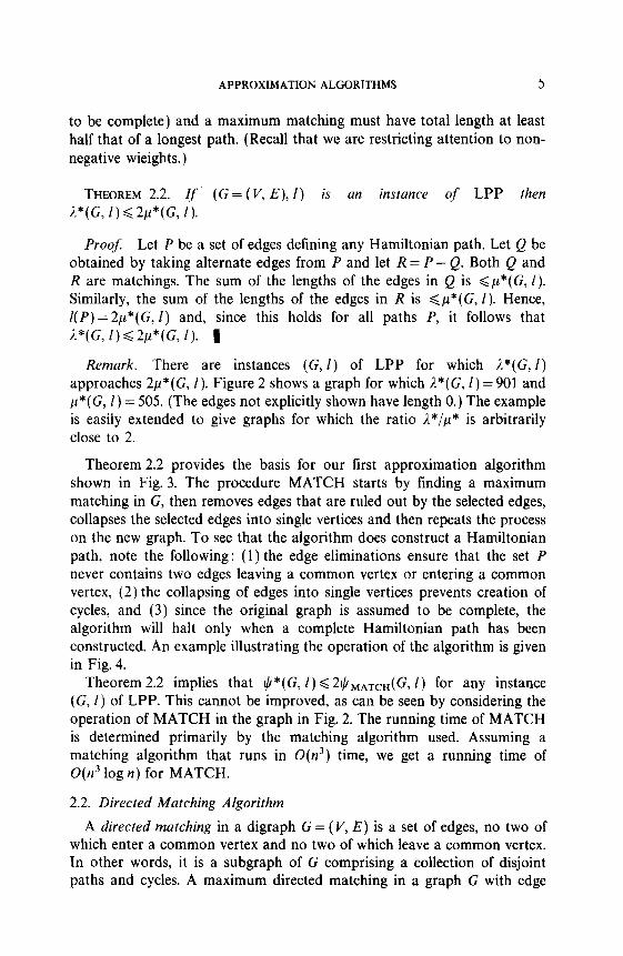
THEOREM 2.2. If’ (G = (V, E), I) is an instance of LPP then A*(G, 1) <2p*(G, I).

Proof: Let P be a set of edges defining any Hamiltonian path. Let Q be obtained by taking alternate edges from P and let R = P - Q. Both Q and R are matchings. The sum of the lengths of the edges in Q is <p*(G, E). Similarly, the sum of the lengths of the edges in R is <p*(G, I). Hence, I(P) = 2p*(G, E) and, since this holds for all paths P, it follows that ;l*(G, 1) d 2p*(G, I). 1

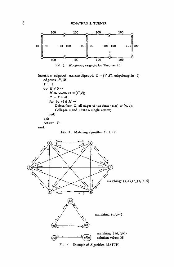
Remark. There are instances (G, 1) of LPP for which ;l*(G, 1) approaches 2p*(G, 1). Figure 2 shows a graph for which I*(G, 1) = 901 and p*(G, 1) = 505. (The edges not explicitly shown have length 0.) The example is easily extended to give graphs for which the ratio 2*/p* is arbitrarily close to 2.

Theorem 2.2 provides the basis for our first approximation algorithm shown in Fig. 3. The procedure MATCH starts by finding a maximum matching in G, then removes edges that are ruled out by the selected edges, collapses the selected edges into single vertices and then repeats the process on the new graph. To see that the algorithm does construct a Hamiltonian path, note the following: (1) the edge eliminations ensure that the set P never contains two edges leaving a common vertex or entering a common vertex, (2) the collapsing of edges into single vertices prevents creation of cycles, and (3) since the original graph is assumed to be complete, the algorithm will halt only when a complete Hamiltonian path has been constructed. An example illustrating the operation of the algorithm is given in Fig. 4.

Theorem 2.2 implies that +*(G, I) < 2$MATCH(G, I) for any instance (G, I) of LPP. This cannot be improved, as can be seen by considering the operation of MATCH in the graph in Fig. 2. The running time of MATCH is determined primarily by the matching algorithm used. Assuming a matching algorithm that runs in 0(n3) time, we get a running time of O(n3 log n) for MATCH.

2.2. Directed Matching Algorithm

A directed matching in a digraph G = (V, E) is a set of edges, no two of which enter a common vertex and no two of which leave a common vertex. In other words, it is a subgraph of G comprising a collection of disjoint paths and cycles. A maximum directed matching in a graph G with edge

JONATHAN S. TURNER

FIG. 2. Worst-case example for Theorem 2.2.

function edgeset MATcE(digraph G = (V,E), edgelengths !)

edgeset P, Id; P := 0; do E#Q-+

h!i := MAXMATCH(G,~);

P:=PuM; for (u,v)EM+

Delete from G, all edges of the form (u, z) or (y, v);

Collapse u and v into a single vertex;

rof;

od; return P;

end;

FIG. 3. Matching algorithm for LPP.

matching: (cf, ba)

@5- -c--J --+ cj-ba matching: (ed, cfba)

solution value: 35

FIG. 4. Example of Algorithm MATCH.


lengths l(e) is a directed matching M that maximizes I(M). We define 6*(G, I) = max, 1(M) to be the value of a maximum directed matching (where in this case, M ranges over all directed matchings of G). There are algorithms for finding a maximum directed matchings having running times of CJ(n5’2) (Tarjan, 1983).

Given any matching M, let M- be a subset of A4 obtained by discarding a least cost edge from each cycle in M. Our next algorithm for LPP is based on the observation contained in the next theorem.

THEOREM 2.3. Let (G = (V, E), I) be an instance of LPP, let A4 be a maximum directed matching of G and let k be the minimum number of edges in any cycle defined by M. A*(G, 1) 6 (k/(k- 1)) I(,%-). In particular, A*(G,I)<2l(M-).

ProoJ Let P be a set of edges defining a path and let M be a maximum directed matching. Notice that P is a directed matching and hence Z(P) < 1(M). Let C be a cycle in M with h edges and let C- be a path obtained by discarding a minimum length edge from C,

Also, for every path R E M, l(R) < (k/(k - 1)) I(R). Summing over all paths and cycles in M yields I(M) < (k/(k - 1)) /(Me). Since this is true for all paths P and since Z(P) < Z(M), I*(G, 1) < (k/(k - 1)) I(M-). 1

Remark. There are instances (G, I) of LPP for which 1*(G, I) approaches 2Z(M-). Consider for example, the graph shown in Fig. 2. For this graph I*(G, I) = 901 and the optimum directed matching consists of five cycles each having two edges and length 201. When the cycles are broken, we have Z(M- ) = 505. The example is easily extended to give graphs for which the ratio A*(G, I)/Z(M-) is arbitrarily close to 2.

We note that 6*(G, I) 2 A*(G, I). Hence, it provides a measure of how close a given solution is to optimal. We expect that the solutions obtained by breaking cycles will often be much closer to optimal than the bound in the theorem implies.

Theorem 2.3 provides the basis for our next approximation algorithm for LPP, shown in Fig. 5. This algorithm constructs a maximum directed matching M in G, then breaks all the cycles in M and constructs a new graph in which the paths of M correspond to vertices. It then proceeds by finding a maximum directed matching in the new graph, continuing in this fashion until a Hamiltonian path in the original graph has been found. To verify that the algorithm does construct a Hamiltonian path, it suffices to note the following: (1) the edge eliminations ensure that the set P never

JONATHAN S. TURNER

function edgeset DIMATCIi(digraph G = (V,E), edgelengths f)

edgeset P, M; P := 0; do E#Q-,

M := MAXDIMATCII(G,f);

M- := M - one least cost edge from each cycle of M;

P:= PUM-; for each path (~1,. . . , u,) E M- -+

Delete from G, all edges of the form (q, z), 2 5 i 5 r;

Delete from G, all edges of the form (z,‘u;), 1 5 i 5 r - 1;

Delete from G the edge (q, ul), if present; Collapse the path into a single vertex;

rof;

od;

return P; end;

FIG. 5. Directed matching algorithm for LPP.

contains two edges leaving a common vertex or entering a common vertex, (2) cycles formed are explicitly broken and the broken edges removed from the graph, and (3) since the original graph is assumed to be complete, the algorithm will halt only when a complete Hamiltonian path has been constructed. An example illustrating the operation of the algorithm is given in Fig. 6.

Theorem 2.3 implies that $*(G, I) < 2t401MATCH(G, I) for any instance (G, I) of LPP. This cannot be improved, as can be seen by considering the operation of MATCH on the graph in Fig. 2. The running time of

directed matching:

(4 cP4, (cfba, 4

6olution value: 35

FIG. 6. Example of Algorithm DIMATCH.


DIMATCH is determined primarily by the directed matching algorithm used. Assuming an algorithm that runs in O(n5’*) time, we get a running time of O(n ‘I2 log n) for DIMATCH.

DIMATCH is essentially an adaptation of an algorithm for the asymmetric traveling salesman problem (TSP) by Karp (1979). Karp’s algorithm has poor worst-case performance for TSP, but performs well in a probabilistic sense for instances in which inter-city distances are selected uniformly on the interval [0, 11. We have simply adapted his algorithm to the longest path problem (simplifying it slightly in the process), and obser- ved that its worst-case performance is provably good in this context.

2.3. Greedy Algorithm

The algorithms considered above are both fairly complicated and time consuming because they require the calculation of maximum weighted matchings. Another algorithm that is worth considering is the simple greedy algorithm that scans the edges in non-increasing order of length and selects an edge (u, u) if it has not previously selected an edge of the form (u, x) or ( y, u) and if the collection of paths constructed so far does not include a path from u to U. On the graph in Fig. 6, this algorithm selects the edges (c, f), (6, a), (e, d), (A b), (d, c) in that order. The next theorem gives a worst-case bound on the performance of the greedy algorithm.

THEOREM 2.4. If (G, 1) is an instance of LPP then L*(G, I) < 31 PGREEIAG 1).

Proof Let F be the set of edges in some optimum solution to (G, I). Let H= {h,, . . . . h,} be the set of edges chosen by the greedy algorithm in the order in which they were selected (that is, h, was selected first, h, second, and so forth).

We say an edge is permissible at some stage of the execution of the algorithm if its selection has not been precluded by earlier selections. Define Hi to be the set of edges which are permissible just before hi is selected, but not permissible after hi is selected.

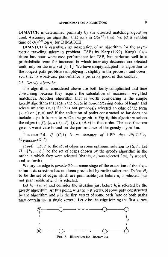
Let hi = (w, y) and consider the situation just before hi is selected by the greedy algorithm. At this point, w is the last vertex of some path constructed by the algorithm and y is the first vertex of some path (one or both paths may contain just a single vertex). Let e be the edge joining the first vertex

n -----o---Q

---+---..~

FIG. 7. Illustration for Theorem 2.4.


100 0 100 100 -@----zz- 0

101

FIG. 8. Worst-case example for PGREEDY.

on the path containing w to the last vertex on the path containing y, as shown in Fig. 7.

If e is permissible before the selection of hi then it is a member of Hi. All other members of Hi have the form (w, z) or the form (x, y). Note that F can contain at most one edge of the form (w, z) and at most one edge of the form (w, z) and at most one edge of the form (x, y). Hence, IFnH;l<3.

Next, note that I(hi) = max(l(e) (e E Hi} and that (Hi, . . . . H,) is a parti- tion of E. Consequently, for in [l, s], l(Fn Hi) < 3Z(hi) and

I(F)= i l(FnHi)<3 i I(hj)=31(H). 1 i=l i=l

Figure 8 gives an example graph showing that the bound of Theorem 2.4 cannot be improved. (The edges not shown have length 0.) PGREEDY finds a solution of length 101, while the optimal solution has length 300. Figure 9 is a sletch of an implementation of the greedy algorithm. Upon return the mappings left and right give the left and right neighbors of each vertex in the solution path. If left(u) is null, then righted(u) gives the vertex at the end of the path containing vertex u in the current partial solution; leftend is similar. The running time for this implementation is O(n2 log n).

function edgeset PGREEDY(digraph G = (V, E), edgelengths e,

mapping le& right : V H V U {null})

vertex U,V; mapping leftend,rightend : V H V; for ?LEVd

Zeft(u),right(u) := null;

Zeftend(u),+ightend(u) := u; r0f;

Sort E from longest to shortest;

for (u,v)~E+ if right(u) = null and left(u) = null and u # Zeftend(u) -+

right(u), left(v) := u, u; tightend(Ieftend(u)) := tightend( leftend(rightend(v)) := leftend(

fi; rof;

return S; end

FIG. 9. Greedy algorithm for LPP.


3. A GREEDY ALGORITHM FOR SCS

The greedy algorithm for the longest path problem can be restated for SCS as follows. Given a non-empty set of strings S, repeat the following step until S contains just one string.

Select a pair of strings sl, s2 E S that maximizes $(si, sZ). Remove s, and s2 from S, replacing them with s1 0 s2.

We refer to this algorithm as SGREEDY. Gallant (1982) claims that 4 sGREEDY(S) < (3/2) d*(S). This is not in fact true, as can be seen by considering the set of strings

S = { abcbcbcbcg, cbcbcbcbc, bcbcbcbcbd)

for which qf~ sGREEDY(S) = 20 > $4*(S) = 19.5. One can easily generalize this example to show that there is no constant c< 2 for which 4 sGREEDY(S) < c$*(S). We currently do not know if there is some constant c > 2 for which &oREEDY(S) < cd*(S).

On the other hand, Theorem 2.4 allows us to conclude that e*(s) G 395 sGREEDY(S). In fact, we can improve the constant factor to 2 by noting that the instances of LPP that arise from the transformation from SCS have a special structure which is decribed in the following lemma.

LEMMA 3.1. Let S be any set of strings and let (G, Z)=LPP(S). If {w, x, y, z} c V with Z(w, y)=max{l(w, y), Z(w, z), 1(x, y), Z(x, z)> then 4w, Y) + 4x, z) 2 4w z) + 0, y).

Proof. Identify w, x, y, z with the corresponding strings in S and let a=I(w, y), /I=f(x,z), y=l(w,z), 6=I(x, y). Note that if cray+6 the result follows immediately. We will assume therefore that c1< y + 6. Figure 10 illustrates the situation described in the lemma.

We define some notation for designating substrings. If s = a, . . . a, is a string, s[i] denotes the symbol ai if i > 0 and a, + i+ 1 if i < 0. The notation s[i,j] denotes the substring s[i] . ..s[j].

471 w z z t I

7 6

Bl

4-4 4-71 WI

a P Yb - + 11 7 YPI Ybl Y I I I

4-61 Y .z z-

FIG. 10. Illustration for Lemma 3.1.


By definition of G,

WC--CL, -1l=Y[l,@l

WC-Y, -1l=zCLyl XC-d, -l]=y[1,6].

(1)

(2)

(3)

Also, w[-y]=y[cl--y+l]. From this we find

z[l,r+6-a]=w[-y,6-cl-l] from (2), a < y + 6 and IX B 6,

=y[a-y-t LS] from (1)

=x[a-y-6, -11 from (3).

Hence, fl=$(x,z)>y+6--a. 1

THEOREM 3.1. Let S be any set of strings. rl/*(S) Q 21,h,,,,,,,(S).

Proof. Let (G, !)=LPP(S). Let H= {hi, . . . . h,} be the set of edges chosen by the greedy algorithm in the order in which they were selected (that is, h, was selected first, h2 second, and so forth). Define n* = I(P) - l({h,, ...y hi}), h w ere P is a longest path that includes {hi, . . . hi}. We show that for in [l, s], A,*_ i < 21(hi) + A,*. Since, $*(S) = A,*, repeated expansion of this inequality implies the theorem.

Let hi < (w, y) and let X= P - {hi, . . . . hip i }, where P is a longest path that includes {hi, . . . . hip,} (so /(X)=&+-i). By definition of the greedy algorithm, I(w, y) = max{ I(e) 1 e E X). At most three edges of X are not permissible after hi is selected. It at most two become impermissible, then 1-T </Ii*_, - 21(w, JJ) as desired. If three edges become impermissible then one must have the form (w, z) with z # y, another the form (x, y) with x # w and the third one, e joins the last vertex on the path containing y with the first vertex on the path containing w. This means that xv {h,, . . . . hi-l} contains a path from x to z, which in turn means that (x, z) is permissible after (w, y) is selected. Consequently,

Ai 2 I(X) - 4 {(x, y), (w, z), e}) + 4, z).

By Lemma 3.1, I( w, y) + l(x, z) 3 I( w, z) + 1(x, y), so

[(x, y) + I(w, z) + l(e) - 4x, z) d 24w, y)

which implies n* 3 A,*_ i - 21(w, y). 1

The bound given by Theorem 3.1 cannot be improved as can be seen by considering the set of strings mentioned at the beginning of this section.


The improvement obtained for the greedy algorithm on strings raises the question of whether or not the bounds for the other approximation algorithms treated in Section 2 can be improved. It turns out that they cannot. If we define

S = (akxbk, bkxck, ckxdk, dkxek, ekxf k,

bk ~ ‘xakx, ck ~ I xbkx, dkp ‘xckx, ek- ‘xdkx, fkxekx)

and (G, [) = LPP(S), we find that I*(G, I) = 9k, lMATCH(G, I)= A. nIMATCW = 5(k + 1). The example can be extended the make the ratios 2*/n MATCH and 2*/iDIh4ATCH arbitrarily close to 2.

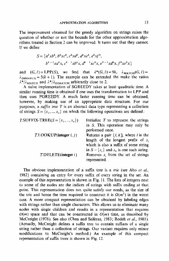
A naive implementation of SGREEDY takes at least quadratic time. A similar running time is obtained if one uses the transformation to LPP and then uses PGREEDY. A much faster running time can be obtained, however, by making use of an appropriate data structure. For our purposes, a suffix tree T is an abstract data type representing a collection of strings S = {s, , . . . . s,} on which the following operations are defined:

T.SUFFIX-TREE(S= {s,, . . . . s,,}) Initialize T to represent the strings in S. This operation may only be performed once.

T.LOOKUP(integer i, j) Returns a pair [l, k], where 1 is the length of the longest prefix of s, which is also a suffix of some string in S- {s, } and Sk is one such String.

T.DELETE( integer i ) Removes s, from the set of strings represented.

The obvious implementation of a suffix tree is a trie (see Aho et al., 1982) containing an entry for every s&ix of every string in the set. An example of this representation is shown in Fig. 11. The lists of integers next to some of the nodes are the indices of strings with suffix ending at that point. This representation does not quite satisfy our needs, as the size of the trie and hence the time required to construct it is Q(m2) in the worst case. A more compact representation can be obtained by labeling edges with strings rather than single characters. This allows us to eliminate many nodes with single children and results in a representation that requires O(m) space and that can be constructed in O(m) time, as described by McCreight (1976). See also (Chen and Seiferas, 1983; Rodeh et al., 1981). (Actually, McCreight defines a suffix tree to contain suffixes of a single string rather than a collection of strings. Our variant requires only minor modifications to McCreight’s method.) An example of this compact representation of suffix trees is shown in Fig. 12.


FIG. 11. Example of trie representation for a suffix tree.

We perform deletion in suffix trees using lazy deletion. That is, to delete a string si, we simply mark it deleted in an auxiliary bit vector maintained for this purpose. When a lookup operation is performed, we perform a probe in the tree to find the longest match. Let u be the node at which the probe terminates. The list of matching strings at u is scanned and any that are marked deleted are removed from the list. If this makes the list empty and u has no children, then u is removed from the tree. If no acceptable match can be found in the list, the search continues at the parent of U.

The time required for a single lookup operation may well exceed the length of the string being searched for. However, any excess time is spent deleting list entries. Since there are initially m + n list entries in the whole tree, the time spent on any sequence of lookups is O(m) plus the sum of the lengths of all strings being searched for.

sl = bbaca 82 = aabac SJ = acacc ~1 = acbba sg = bacbb

FIG. 12. Example of compacted trie representation.


We say that a sequence of lookup and delete operations is monotonic if for every i, j, k with j # k, whenever the sequence contains the operation T.LOOKUP(i, j) and later on the operation T.LOOKUP(i, k) it contains the operation T.DELETE(j) between the other two.

We can speed up a monotonic sequence of operations by maintaining, for each string, a pointer to the node where the most recent lookup for that string ended. This allows us to avoid the initial prove of the tree when we perform a lookup operation. Instead, we use the pointer to go straight to the node where the last probe ended and search up from that node if necessary. In this way, we can perform a monotonic sequence of I operations in O(m + r) time.

This analysis assumes that the symbol alphabet is small enough that it is reasonable to use a vector of pointers to children in each node, indexed by the first symbol of the strings labeling the edges. If a large alphabet is needed, a hash table may be used. Another option is to use a variant on Sleator and Tarjan’s lexicographic splay tree (1985). With this representation, the time required to perform a sequence of operations is O(m), plus the sum of the lengths of the strings being searched for, plus O(log m) per operation. For a monotonic sequence of r operations the time is O(m + r log m).

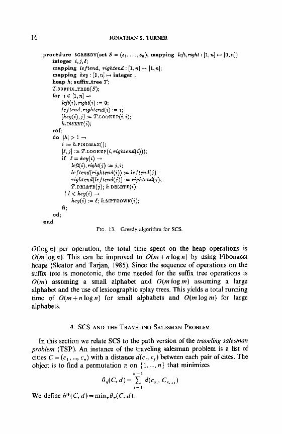
An efficient implementation of the greedy algorithm for strings is shown in Fig. 13. The algorithm does not explicitly combine strings, but keeps track of the decisions made using the two mappings f@(i), right(i) which give the left and right neighbors of string i in the solution constructed so far. A value of 0 means that there is no neighbor. The solution is returned in these mappings. If a string i has no left neighbor yet, righted(i) is the original string which is currently rightmost in the piece of the partial solution that contains i; leftend is similar.

The heap h, is used to determine which pair of strings should be combined next. Each string is entered in h with the key being the length of the best match for h. As the algorithm proceeds, certain matches become unavailable and the values of key may become invalid. Consequently, whenever a string si is selected from h, a new lookup operation is performed in T. If the result of that operation is a match of the same length as key(i), the strings are combined. If the lookup results in a shorter match, the value of key(i) is changed and the position of si in the heap is adjusted to reflect the new value. Note that a string is deleted from the heap once it is successfully matched with another string on its left end. Similarly, a string is deleted from the suffix tree once it is matched with a string on the right.

The running time of the algorithm is dominated by the operations on the various data structures within the main loop. The number of iterations of the main loop is O(m) in the worst case. Since the heap operations are

143/W-2


procedure SGREEDY(set s = (~1 , . . . ,+.), mapping left, right : [I, n] H [0, n]) integer i, j,l; mapping leftend, tightend : [l,n] H [l,n]; mapping key : [l, n] w integer ; heap h; suffix-tree T; T.SUFFIX-TREE(S); for i E [l,n] 4

ZeNi), right(i) := 0;

leftend, righted(i) := i;

[key(i),j] := T.LOOKUP(i,i); ~.INsERT(~);

rof;

do jhj > 1 +

i := ~.PINDMAX(); [f,j] := T.LOOKUP(i,rightend(i)));

if .! = key(i) -+

left(i), right(j) := j, i;

ieftend(rightend(i)) := leftend( rightend(leftend(j)) := righted(j);

T.DELETE(j); ~.DELETE(~); ) 1 < key(i) -+

key(i) := t?; ~.SIFTDOWN(~);

fi; od;

end FIG. 13. Greedy algorithm for SCS.

O(log n) per operation, the total time spent on the heap operations is O(m log n). This can be improved to O(m +n log n) by using Fibonacci heaps (Sleator and Tarjan, 1985). Since the sequence of operations on the suffix tree is monotonic, the time needed for the suffix tree operations is O(m) assuming a small alphabet and O(m log m) assuming a large alphabet and the use of lexicographic splay trees. This yields a total running time of O(m+n log n) for small alphabets and O(m log m) for large alphabets.

4. SCS AND THE TRAVELING SALESMAN PROBLEM

In this section we relate SCS to the path version of the traveling salesman problem (TSP). An instance of the traveling salesman problem is a list of cities C = (ci, . . . . c,) with a distance d(ci, cl) between each pair of cites. The object is to find a permutation rc on { 1, . . . . n} that minimizes

n-1

Qn(C9 d) = 1 4cn,> cc,+,) i= 1

We define O*(C, d) = min,B,(C, d).


Let s= (s,, . ..) s,) be an instance of SCS. We define TSP(s,, .,., s,) to be an instance (C, d) to TSP with C= (c,, . . . . c,, c,+ 1) and

lsil - +tsi, sj) 1 <i<n, 1 <j<n, i#j,

d(ci, cj) = lsil l<i<n,j=n+l,

IISII i=n+ 1,l dj<n.

An example of this transformation is given in Fig. 14. Note that in general, if rr satisfies 19,( C, d) = O*( C, d) then nn + I = c, + I .

THEOREM 4.1. Let S= (s,, . . . . s,) be an instance ofSCS, (C, d) = TSP(S) and let z be a permutation on { 1, . . . . n, n + 1 } to (cl, . . . . c,, c,+ 1) for which 7r n+ 1 = n + 1. Then t9,(C, d) =4,,(S), w ere h 71’ is the restriction of 71 to { 1, . . . . n}. In particular, O*(C, d) = d*(S).

ProoJ:

e,(C, 4 = i d(c,,, c,,+J = ‘f’ b,,I - Icl(s ,=l i= 1

O*(C, d) = b*(S) follows from the observation that any optimum solution n for (C,d) must have r~,+~=c,,+~. 1

Theorem 4.1 implies that any good approximation algorithm for this version of the traveling salesman problem is a good approximation algorithm for SCS as well. The particular instances of TSP constructed by the transformation defined above have some special properties. First, they may be asymmetric; that is, d(ci, c,) need not equal d(cj, ci). The next theorem shows that they obey the so-called triangle inequality.

S = (cbadef ,f cbade, adef cd)

FIG. 14. Example of transformation from SCS to TSP.

18 JONATHANS.TURNER

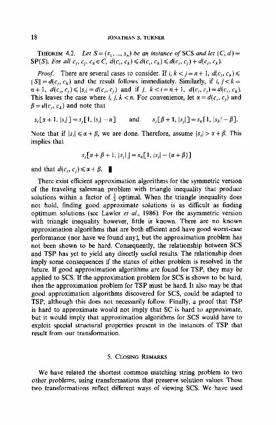
THEOREM 4.2. Let S= (sl, . . . . s,) be an instance of SCS and let (C, d) = SP(S). FOI' all Ci, Cjj ck E C, d(ci, Ck) < d(ci, ck) < d(c,, Cj) -I- d(ci, Ck).

ProoJ: There are several cases to consider. If i, k < j = n + 1, d(c,, ck) < ljS]j = d(cj, ck) and the result follows immediately. Similarly, if i, j< k = n + 1, d(ci, c,) < Jsil = d(cj, ci) and if j, k < i= n + 1, d(c,, cj) = d(c,, ck). This leaves the case where i, j, k < n. For convenience, let a = d(c;, c,) and /?=d(c,, ck) and note that

Si[a+ 1, lSil]=Sj[l, JSil -a] and sjCB+ 1, IsjII=Sk[l, Is/cl -PI.

Note that if 1.~~1 <a + /?, we are done. Therefore, assume 1.~~1 > a + B. This implies that

and that d(c,, c,) 6 a + fi. 1

There exist efficient approximation algorithms for the symmetric version of the traveling salesman problem with triangle inequality that produce solutions within a factor of 3 optimal. When the triangle inequality does not hold, finding good approximate solutions is as difficult as finding optimum solutions (see Lawler et al., 1986). For the asymmetric version with triangle inequality however, little is known. There are no known approximation algorithms that are both efftcient and have good worst-case performance (nor have we found any), but the approximation problem has not been shown to be hard. Consequently, the relationship between SCS and TSP has yet to yield any directly useful results. The relationship does imply some consequences if the status of either problem is resolved in the future. If good approximation algorithms are found for TSP, they may be applied to SCS. If the approximation problem for SCS is shown to be hard, then the approximation problem for TSP must be hard. It also may be that good approximation algorithms discovered for SCS, could be adapted to TSP, although this does not necessarily follow. Finally, a proof that TSP is hard to approximate would not imply that SC is hard to approximate, but it would imply that approximation algorithms for SCS would have to exploit special structural properties present in the instances of TSP that result from our transformation.

5. CLOSING REMARKS

We have related the shortest common matching string problem to two other problems, using transformations that preserve solution values. These two transformations reflect different ways of viewing SCS. We have used


the transformations to gain insight into the problem of approximating SCS and have discovered several algorithms that have provably good performance with respect to the overlap measure. The best of these is the string version of the greedy algorithm for which we have described an efficient implementation using suffix trees.

While we have shown that the string version of the greedy algorithm has good worst-case performance with respect to the overlap measure, we cannot determine its performance with respect to the length measure. We know that it can be off by as much as a factor of 2 with respect to the length measure, but we do not know if it can be worse than this. One open problem then, is to resolve this issue.

Although, we have been unable to make use of the relationship between SCS and TSP to advantage, we feel that it may yet prove useful. More generally, we think that the use of transformations that preserve solution values can be used to extend the application of known approximation algorithms to new domains. A methodical development of such transformations could provide many useful results.

Another worthwhile line of investigation for future research is to study the probable performance of the various approximation algorithms using appropriate probability models. It appears likely, for example, that the directed matching algorithm for the longest path problem performs much better than its worst-case bound would indicate for a wide class of natural probability models. Similarly, one would expect the greedy algorithm to perform well in a probabilistic sense for many useful probability models.

RECEIVED August 3, 1987; ACCEPTED November 23, 1988

REFERENCES

AHO, A. V., HOPCROFT, J. E., AND ULLMAN. J. D. (1982), “Data Structures and Algorithms,” Addison-Wesley, Reading, MA.

CHEN, M. T., AND SEIFEXAS, J. I. (1983), “Efficient and Elegant Subword-Tree Construction,” Technical Report TR 129, 12/83, University of Rochester, Computer Science Department,

GALLANT, J. K., MAIER, D. STORER, J. A. (1980), On finding minimal length supcrstrings, J. Comput. System Sci. 20, No. 1 50-58.

GALLANT, J. K. (1982), “String Compression Algorithms,” PhD. dissertation, Princeton University, Department of Electrical Engineering and Computer Science.

GINGERAS, T. R., MILAO, J. P., SCIAKY, AND R. J. ROBERTS (1979), Computer programs for the assembly of DNA sequences, Nucleic Acids Res. 7, 529-545.

KARP, R. M. (1979), A patching algorithm for the nonsymmetric traveling salesman problem, SIAM J. Compur. 8, No. 4, 561-573.

LAWLER, E. L., LENSTRA, J. K.. AND RINNO~Y KAN, A.H.G. (Eds.) (1986), “The Traveling Salesman Problem,” Wiley, New York.

MAIER, D., AND STORER. J. A. (1977). “A Note on the Complexity of the Superstring


Problem,” Technical Report 233, Department of Electrical Engineering and Computer Science, Princeton University.

MAYNE, A., AND JAMES, E. B. (1975), Information compression by factorising common strings, Compur. J. 18, 157-160.

MCCREIGHT, E. M. (1976), A space-economical suffix tree construction algorithm, J. Assoc. Comput. Mach. 23, 262-272.

RODEH, M., PRAY, V. R., AND EVEN, S. (1981) Linear algorithm for data compression via string matching, J. Assoc. Comput. Mach. 28, 16-24.

SHAPIRO, M. B. (1967) An algorithm for reconstructing protein and RNA sequences, J. Assoc. Comput. Mach. 14, 72&731.

SLEATOR, D. D., AND TARJAN, R. E. (1985) Self-adjusting binary search trees, J. Assoc. Comput. Mach. 32, 652-686.

STEFIK, M. (1978), Inferring DNA structures from segmentation data, Artif: Intelligence, vol. 11, 1978, 85-114.

STORER, J. A., AND SZYMANSKI, T. Cl. (1982), Data compression via textual substitution, J. Assoc. Comput. Mach. 29, 928-951.

TARJAN, R. E. (1983) “Data Structures and Network Algorithms,” Sot. Indus. Appl. Math., Philadelphia.

Approximation Algorithms for the Shortest Common ... · shortest possible string that contains...

Documents

Transcript of Approximation Algorithms for the Shortest Common ... · shortest possible string that contains...