Approximating the Stochastic Knapsack Problem:

The Benefit of Adaptivity

Brian C. Dean∗ Michel X. Goemans† Jan Vondrak‡

June 6, 2008

Abstract

We consider a stochastic variant of the NP-hard 0/1 knapsack problem in which item values aredeterministic and item sizes are independent random variables with known, arbitrary distributions. Itemsare placed in the knapsack sequentially, and the act of placing an item in the knapsack instantiates itssize. Our goal is to compute a solution “policy” that maximizes the expected value of items successfullyplaced in the knapsack, where the final overflowing item contributes no value. We consider both non-adaptive policies (that designate a priori a fixed sequence of items to insert) and adaptive policies (thatcan make dynamic choices based on the instantiated sizes of items placed in the knapsack thus far).An important facet of our work lies in characterizing the benefit of adaptivity. For this purpose weadvocate the use of a measure called the adaptivity gap: the ratio of the expected value obtained by anoptimal adaptive policy to that obtained by an optimal non-adaptive policy. We bound the adaptivitygap of the Stochastic Knapsack problem by demonstrating a polynomial-time algorithm that computesa non-adaptive policy whose expected value approximates that of an optimal adaptive policy to withina factor of 4. We also devise a polynomial-time adaptive policy that approximates the optimal adaptivepolicy to within a factor of 3 + ε for any constant ε > 0.

1 Introduction

The classical NP-hard knapsack problem takes as input a set of n items with values v1 . . . vn and sizess1 . . . sn, and asks us to compute a maximum-value subset of these items whose total size is at most 1.Among the many applications of this problem, we find the following common scheduling problem: givena set of n jobs, each with a known value and duration, compute a maximum-value subset of jobs one canschedule by a fixed deadline on a single machine. In practice, it is often the case that the duration of a job isnot known precisely until after the job is completed; beforehand, it is known only in terms of a probabilitydistribution. This motivates us to consider a stochastic variant of the knapsack problem in which item valuesare deterministic and sizes are independent random variables with known, completely arbitrary distributions.The actual size of an item is unknown until we instantiate it by attempting to place it in the knapsack. Witha goal of maximizing the expected value of items successfully placed in the knapsack, we seek to design asolution “policy” for sequentially inserting items until the capacity is eventually exceeded. At the momentwhen the capacity overflows, the policy terminates.

Formally, if [n] := {1, 2, . . . , n} indexes a set of n items, then an solution policy is a mapping 2[n]×[0, 1] → [n]specifying the next item to insert into the knapsack given the set of remaining (uninstantiated) availableitems as well as the remaining capacity in the knapsack. We typically represent a solution policy in terms ofan algorithm that implements this mapping, and we can visualize such an algorithm in terms of a decisiontree as shown in Figure 1. As illustrated by the instances shown in the figure, an optimal policy may need

∗McAdams Hall, Box 340974, Clemson University, Clemson, SC, 29634†MIT, Department of Mathematics, Cambridge, MA, 02139‡Department of Mathematics, Fine Hall, Washington Rd, Princeton, NJ, 08644

1

0 (prob ) 1+ (prob 1− )

s = 0.82

s = 0.93

3s = 0.4

Prob = 1/2Value = 2

Item

123

0.2 (prob 1/2) 0.6 (prob 1/2)0.8 (prob 1)0.4 (prob 1/2) 0.9 (prob 1/2)

Size Distribution (capacity = 1)

Size Distribution (capacity = 1)Item

123

Value

1

0 (prob 1/2) 1 (prob 1/2)εε 1 (prob 1)

εε ε

(b)

Insert 1

Insert 2

Insert 3

Value = 2

Value = 1Prob = 1/4

Prob = 1/4

s =

0.2

s = 0.6

1

1

(a)

(c)

Figure 1: Instances of the stochastic knapsack problem. For (a), an optimal non-adaptive policy inserts items in the order 1, 2, 3, and achieves expected value 1.5.An optimal adaptive policy, shown as a decision tree in (b), achieves an expectedvalue of 1.75, for an adaptivity gap of 7/6. The instance in (c) has adaptivitygap arbitrarily close to 5/4: an optimal non-adaptive policy inserts items in theorder 1, 3, 2 for an expected value of 2ε + 1

2ε2, and an optimal adaptive policy

inserts item 1 followed by items 2 and 3 (if s1 = 0) or item 3 (if s1 = 1), for anexpected value of 2.5ε.

to be adaptive, making decisions in a dynamic fashion in reaction to the instantiated sizes of items alreadyplaced in the knapsack. By contrast, a non-adaptive policy specifies an entire solution in advance, making nofurther decisions as items are being inserted. In other words, a non-adaptive policy is just a fixed ordering ofthe items to insert into the knapsack. It is at least NP-hard to compute optimal adaptive and non-adaptivepolicies for the Stochastic Knapsack problem, since both of these problems reduce to the classical knapsackproblem in the deterministic case.

There are many problems in stochastic combinatorial optimization for which one could consider designingeither adaptive or non-adaptive solution policies. In particular, these are problems in which a solution isincrementally constructed via a series of decisions, each of which establishes a small part of the total solutionand also results in the instantiation of a small part the problem instance. When trying to solve such aproblem, it is often a more complicated undertaking to design a good adaptive policy, but this might give ussubstantially better performance than a non-adaptive policy. To quantify the benefit we gain from adaptivity,we advocate the use of a measure we call the adaptivity gap, which measures the maximum (i.e., worst case)ratio over all instances of a problem of the expected value obtained by an optimal adaptive policy to theexpected value obtained by an optimal non-adaptive policy. One of the main results in this paper is a proofthat the adaptivity gap of the Stochastic Knapsack problem is at most 4, so we only lose a small constantfactor by considering non-adaptive policies. Adaptivity gap plays a similar role to the integrality gap of afractional relaxation by telling us the best approximation bound we can hope to achieve by considering aparticular simple class of solutions. Also, like the integrality gap, one can study the adaptivity gap of aproblem independently of any considerations of algorithmic efficiency.

1.1 Outline of Results

In this paper we provide both non-adaptive and adaptive approximation algorithms for the Stochastic Knap-sack problem. After giving definitions and preliminary results in Section 2, we present three main approx-imation algorithm results in the following sections. Section 3 describes how we can use a simple linearprogramming relaxation to bound the expected value obtained by an optimal adaptive policy, and we usethis bound in Section 4 to develop a 32/7-approximate non-adaptive policy. We then develop a more sophis-ticated linear programming bound based on a polymatroid in Section 5, and use it in Section 6 to constructa 4-approximate non-adaptive policy. Sections 7 and 8 then describe a (3 + ε)-approximate adaptive policy

2

for any constant ε > 0 (the policy takes polynomial time to make each of its decisions).

In Section 9 we consider what we call the ordered adaptive model. Here, the items must be considered in theorder they are presented in the input, and for each item we can insert it into the knapsack or irrevocablydiscard it (and this decision can be adaptive, depending on the instantiated sizes of items already placedin the knapsack). This model is of interest since we can compute optimal ordered policies in pseudo-polynomial time using dynamic programming in the event that item size distributions are discrete, just asthe deterministic knapsack problem is commonly approached with dynamic programming if item sizes arediscrete. A natural and potentially difficult question with this model is how one should choose the initialordering of the items. If we start with the ordering produced by our 4-approximate non-adaptive policy, theoptimal ordered adaptive policy will have an expected value within a factor of 4 of the optimal adaptivepolicy (and it can potentially be much closer). We show in Section 9 that for any initial ordering of items,the optimal ordered adaptive policy will obtain an expected value that differs by at most a factor of 9.5 fromthat of an optimal adaptive policy.

1.2 Literature Review

The Stochastic Knapsack problem is perhaps best characterized as a scheduling problem, where it couldbe written as 1 | pj ∼ stoch, dj = 1 | E[

∑wjU j ] using the three-field scheduling notation popularized by

Lawler, Lenstra, and Rinnooy Kan [10]. Stochastic scheduling problems, where job durations are randomvariables with known probability distributions, have been studied quite extensively in the literature, datingback as far as 1966 [20]. However, for the objective of scheduling a maximum-value collection of jobs priorto a fixed deadline, all previous research seems to be devoted to characterizing which classes of probabilitydistributions allow an exact optimal solution to be computed in polynomial time. For example, if the sizesof items are exponentially distributed, then Derman et al. [6] prove that the greedy non-adaptive policy thatchooses items in non-increasing order of vi/E[si] is optimal. For extensions and further related results, seealso [18, 7, 3]. To the best of our knowledge, the only stochastic scheduling results to date that considerarbitrary probability distributions and the viewpoint of approximation algorithms tend to focus on differentobjectives, particularly minimizing the sum of weighted completion times — see [16, 23, 26].

The notion of adaptivity is quite prevalent in the stochastic scheduling literature and also in the stochasticprogramming literature (see, e.g., [1]) in general. One of the most popular models for stochastic optimizationis a two-stage model where one commits to a partial solution and then, and then after witnessing theinstantiation of all random quantities present in the instance, computes an appropriate recourse as necessaryto complete the solution. For example, a stochastic version of bin packing in this model would ask us topack a collection of randomly-sized items into the minimum possible number of unit sized bins. In the firststage, we can purchase bins at a discounted price, after which we observe the instantiated sizes of all itemsand then, as a recourse, purchase and additional bins that are needed (at a higher price). For a survey ofapproximation results in the two-stage model, see [12, 19, 22]. By contrast, our model for the StochasticKnapsack problem involves unlimited levels of recourse. The notion of adaptivity gap does not seem tohave received any explicit attention thus far in the literature. Note that the adaptivity gap only applies toproblems for which non-adaptive solutions make sense. Quite a few stochastic optimization problems, suchas the two-stage bin packing example above, are inherently adaptive since one must react to instantiatedinformation in order to ensure the feasibility of the final solution.

Several stochastic variants of the knapsack problem different from ours have been studied in the literature.Stochastic Knapsack problems with deterministic sizes and random values have been studied by severalauthors [2, 11, 24, 25], all of whom consider the objective of computing a fixed set of items fitting in theknapsack that has maximum probability of achieving some target value (in this setting, maximizing expectedvalue is a much simpler, albeit still NP-hard, problem since we can just replace every item’s value with itsexpectation). Several heuristics have been proposed for this variant (e.g. branch-and-bound, preference-order dynamic programming), and adaptivity is not considered by any of the authors. Another somewhatrelated variant, known as the stochastic and dynamic knapsack problem [14, 17], involves items that arriveon-line according to some stochastic process — we do not know the exact characteristics of an item untilit arrives, at which point in time we must irrevocably decide to either accept the item and process it, or

3

discard the item. Two recent papers due to Kleinberg et al. [13] and Goel and Indyk [9] consider a StochasticKnapsack problem with “chance” constraints. Like our model, they consider items with deterministic valuesand random sizes. However, their objective is to find a maximum-value set of items whose probability ofoverflowing the knapsack is at most some specified value p. Kleinberg et al. consider only the case whereitem sizes have a Bernoulli-type distribution (with only two possible sizes for each item), and for this casethey provide a polynomial-time O(log 1/p)-approximation algorithm as well as several pseudo-approximationresults. For item sizes that have Poisson or exponential distributions, Goel and Indyk provide a PTAS, andfor Bernoulli-distributed items they give a quasi-polynomial approximation scheme whose running timedepends polynomially on n and log 1/p.

Kleinberg et al. show that the problem of computing the overflow probability of a set of items, even withBernoulli distributions, is #P-hard. Consequently, it is #P-hard to solve the variant mentioned above withdeterministic sizes and random values, where the goal is to find a set of items whose probability of exceedingsome target value is maximized. To see this, let Be(s, p) denote the Bernoulli distribution taking the value swith probability p and 0 with probability 1− p, and consider a set of items i = 1 . . . n with size distributionsBe(si, pi). In order to compute the overflow probability p∗ of this set of items in a knapsack of capacity1, we construct an instance of the stochastic knapsack problem above with target value 1 and n + 1 items:items i = 1 . . . n have size 1/n and value Be(si, pi), and the last has size 1 and value Be(1, p′). The optimalsolution will contain the first n items if p∗ > p′ or the single last item otherwise, so we can compute p∗ usinga binary search on p′. Note that it is also #P-hard to solve the restricted problem variant with random sizesand deterministic values, where the goal is to find a set of maximum value given a bound on the overflowprobability. Here, we can take a set of items i = 1 . . . n with sizes Be(si, pi) and compute their overflowprobability p∗ by constructing a stochastic knapsack instance with overflow probability threshold p′ and withn items of size Be(si, pi) and unit value. Since the optimal solution to this problem will be the set of allitems (total value n) if and only if p∗ ≤ p′, we can again compute p∗ using a binary search on p′.

In contrast to the results cited above, we do not assume that the distributions of item sizes are exponential,Poisson or Bernoulli; our algorithms work for arbitrary distributions. The results in this paper substantiallyimprove upon the results given in its extended abstract [5], where approximation bounds of 7 and 5 + ε areshown for non-adaptive and adaptive policies. Note that a large part of the analysis in [5] (see also [4]) is nolonger needed in this paper, but the different methods used in that analysis may also be of interest to thereader.

2 Preliminaries

2.1 Definition of the problem

An instance I consists of a collection of n items characterized by size and value. For each item i ∈ [n], letvi ≥ 0 denote its value and si ≥ 0 its size. We assume the vi’s are deterministic while the si’s are independentrandom variables with known, arbitrary distributions. Since our objective is to maximize the expected valueof items placed in the knapsack, we can allow random vi’s as long as they are mutually independent andalso independent from the si’s. In this case, we can simply replace each random vi with its expectation. Inthe following, we consider only deterministic values vi. Also, we assume without loss of generality that ourinstance is scaled so the capacity of the knapsack is 1.

Definition 1 (Adaptive policies). An adaptive policy is a function P : 2[n]× [0, 1] → [n]. The interpretationof P is that given a set of available items J and remaining capacity c, the policy inserts item P(J, c). Thisprocedure is repeated until the knapsack overflows. We denote by val(P) the value obtained for all successfullyinserted items, which is a random variable resulting from the random process of executing the policy P. Wedenote by ADAPT (I) = maxP E[val(P)] the optimum1 expected value obtained by an adaptive policy forinstance I.

Definition 2 (Non-adaptive policies). A non-adaptive policy is an ordering of items O = (i1, i2, i3, . . . , in).1One can show that the supremum implicit in the definition of ADAPT (I) is attained.

4

We denote by val(O) the value obtained for successfully inserted items, when inserted in this order. Wedenote by NONADAPT (I) = maxO E[val(O)] the optimum expected value obtained by a non-adaptivepolicy for instance I.

In other words, a non-adaptive policy is a special case of an adaptive policy P(J, c) which does not dependon the residual capacity c. Thus we always have ADAPT (I) ≥ NONADAPT (I). Our main interest in thispaper is in the relationship of these two quantities. We investigate how much benefit a policy can gain bybeing adaptive, i.e. how large ADAPT (I) can be compared to NONADAPT (I).

Definition 3 (Adaptivity gap). We define the adaptivity gap as

supI

ADAPT (I)NONADAPT (I)

where the supremum is taken over all instances of Stochastic Knapsack.

This concept extends naturally beyond the Stochastic Knapsack problem. It seems natural to study theadaptivity gap for any class of stochastic optimization problems where adaptivity is present [4, 27].

It should be noted that in the definition of the adaptivity gap, there is no reference to computationalefficiency. The quantities ADAPT (I) and NONADAPT (I) are defined in terms of all policies that exist,but it is another question whether an optimal policy can be found algorithmically. Observe that an optimaladaptive policy might be quite complicated in structure; for example, it is not even clear that one can alwayswrite down such a policy using polynomial space.

Example 1. Consider a knapsack of large integral capacity and n unit-value items, half of type A andhalf of type B. Items of type A take size 1, 2, or 3 each with probability p, and then sizes 5, 7, 9, . . . withprobability 2p. Items of type B take size 1 or 2 with probability p, and sizes 4, 6, 8, . . . with probability 2p.If p is sufficiently small, then the optimal policy uses a type A item (if available) if the remaining capacityhas odd parity and a type B item if the remaining capacity has even parity. The decision tree correspondingto an optimal policy would have at least

(n

n/2

)leaves.

Since finding the optimal solution for the deterministic knapsack problem is NP-hard, and some questionsconcerning adaptive policies for Stochastic Knapsack are even PSPACE-hard [5, 27], constructing or char-acterizing an optimal adaptive policy seems very difficult. We seek to design approximation algorithms forthis problem. We measure the quality of an algorithm by comparing its expected value against ADAPT .That is, if A(I) denotes the expected value of our algorithm A on instance I, we say that the performanceguarantee of A is

supI

ADAPT (I)A(I)

.

This measurement of quality differs greatly from the measure we would get from traditional competitiveanalysis of on-line algorithms or its relatives (e.g., [15]). Competitive analysis would have us compare theperformance of A against an unrealistically-powerful optimal algorithm that knows in advance the instanti-ated sizes of all items, so it only allows us to derive very weak guarantees. For example, let Be(p) denotethe Bernoulli probability distribution with parameter p (taking the value zero with probability 1 − p andone with probability p). In an instance with n items, each of size (1 + ε)Be(1/2) and value 1, we haveADAPT ≤ 1 while if we know the instantiated item sizes in advance we could achieve an expected value ofat least n/2 (since we expect n/2 item sizes to instantiate to zero).

For similar reasons, we assume that the decision to insert an item into the knapsack is irrevocable — inthe scheduling interpretation of our problem, we might want the ability to cancel a job after schedulingit but then realizing after some time that, conditioned on the time it has already been processing, itsremaining processing time is likely to be unreasonably large. The same example instance above shows thatif cancellation is allowed, our policies must somehow take advantage of this fact or else we can only hope

5

to obtain an O(1/n) fraction of the expected value of an optimal schedule in the worst case. We do notconsider the variant of Stochastic Knapsack with cancellation in this paper.

2.2 Additional definitions

In the following, we use the following quantity defined for each item:

Definition 4. The mean truncated size of an item i is

µi = E[min{si, 1}].

For a set of items S, we define val(S) =∑

i∈S vi, size(S) =∑

i∈S si and µ(S) =∑

i∈S µi. We refer to µ(S)as the “mass” of set S.

One motivation for this definition is that µ(S) provides a natural bound on the probability that a set ofitems overflows the knapsack capacity.

Lemma 1. Pr[size(S) < 1] ≥ 1− µ(S).

Proof. Pr[size(S) ≥ 1] = Pr[min{size(S), 1} ≥ 1] ≤ E [min{size(S), 1}] ≤ E[∑

i∈S min{si, 1}]

= µ(S).

The mean truncated size is a more useful quantity than E[si] since it is not sensitive to the structure ofsi’s distribution in the range si > 1. In the event that si > 1, the actual value of si is not particularlyrelevant since item i will definitely overflow the knapsack (and therefore contribute no value towards ourobjective). All of our non-adaptive approximation algorithms only look at the mean truncated size µi andthe probability of fitting in an empty knapsack Pr[si ≤ 1] for each item i; no other information about the sizedistributions is used. However, the (3 + ε)-approximate adaptive policy we develop in Section 8 is assumedto know the complete size distributions, just like all adaptive policies in general.

3 Bounding Adaptive Policies

In this section we address the question of how much expected value an adaptive policy can possibly achieve.We show that despite the potential complexity inherent in an optimal adaptive policy, a simple linearprogramming (LP) relaxation can be used to obtain a good bound on its expected value.

Let us fix an adaptive policy P and consider the random set of items A that P inserts successfully into theknapsack. In a deterministic setting, it is clear that µ(A) ≤ 1 for any policy since our capacity is 1. It isperhaps surprising that in the stochastic case, E[µ(A)] can be larger than 1.

Example 2. Suppose we have an infinitely large (random) set of items where each item i has value vi = 1and size si ∼ Be(p). In this case, E[|A|] = 2/p − 1 (since we can insert items until the point where two ofthem instantiate to unit size) and each item i has mean truncated size µi = p, so E[µ(A)] = 2− p. For smallp > 0, this quantity can be arbitrarily close to 2. If we count the first overflowing item as well, we insertmass exactly 2. This is a tight example for the following crucial lemma.

Lemma 2. For any Stochastic Knapsack instance with capacity 1 and any adaptive policy, let A denote the(random) set of items that the policy attempts to insert. Then E[µ(A)] ≤ 2.

Proof. Consider any adaptive policy and denote by At the (random) set of the first t items that it attemptsto insert. (We set A0 = ∅.) Eventually, the policy terminates, either by overflowing the knapsack or byexhausting all the available items. If either event happens upon inserting t′ items, we set At = At′ for all

6

t > t′; note that At′ still contains the first overflowing item. Since the process always terminates like this,we have

E[µ(A)] = limt→∞

E[µ(At)] = supt≥0

E[µ(At)].

Denote by si = min{si, 1} the mean truncated size of item i. Observe∑

i∈Atsi ≤ 2 for all t ≥ 0. This is

because each si is bounded by 1 and we can count at most one item beyond the capacity of 1. We now definea sequence of random variables {Xt}t∈Z+ :

Xt =∑i∈At

(si − µi).

This sequence {Xt} is a martingale: conditioned on a value of Xt and the next inserted item i∗,

E[Xt+1|Xt, i∗] = Xt + E[si∗ ]− µi∗ = Xt.

If no more items are inserted, Xt+1 = Xt trivially. We can therefore remove the conditioning on i∗, soE[Xt+1|Xt] = Xt, and this is the definition of a martingale. We now use the well-known martingale propertythat E[Xt] = E[X0] for any t ≥ 0. In our case, E[Xt] = E[X0] = 0 for any t ≥ 0. As we mentioned,

∑i∈At

si

is always bounded by 2, so Xt ≤ 2 − µ(At). Taking the expectation, 0 = E[Xt] ≤ 2 − E[µ(At)]. ThusE[µ(A)] = supt≥0 E[µ(At)] ≤ 2.

We now show how to bound the value of an optimal adaptive policy using a linear program. We define bywi = vi ·Pr[si ≤ 1] the effective value of item i, which is an upper bound on the expected value a policy cangain if it attempts to insert item i. Consider now the linear programming relaxation for a knapsack problemwith item values wi and item sizes µi, parameterized by the knapsack capacity t:

Φ(t) = max

{∑i

wixi :∑

i

µixi ≤ t, xi ∈ [0, 1]

}.

Note that we use wi instead of vi in the objective for the same reason that we cannot just use vi in thedeterministic case. If we have a deterministic instance with a single item whose size is larger than 1, thenwe cannot use this item in an integral solution but we can use part of it in a fractional solution, giving us anunbounded integrality gap. To fix this issue, we need to appropriately discount the objective value we canobtain from such large items, which leads us to the use of wi in the place of vi. Using the linear programabove, we now arrive at the following bound.

Theorem 1. For any instance of the Stochastic Knapsack problem, ADAPT ≤ Φ(2).

Proof. Consider any adaptive policy P, and as above let A denote the (random) set of items that P attemptsto insert into the knapsack. Consider the vector ~x where xi = Pr[i ∈ A]. The expected mass that P attemptsto insert is E[µ(A)] =

∑i µixi. We know from Lemma 2 that this is bounded by E[µ(A)] ≤ 2, therefore ~x is

a feasible vector and∑

i wixi ≤ Φ(2).

Let fit(i, c) denote the indicator variable of the event that si ≤ c. Let ci denote the capacity remainingwhen P attempts to insert item i. This is a random variable well-defined if i ∈ A. The expected profit foritem i is

E[vi fit(i, ci) | i ∈ A] · Pr[i ∈ A] ≤ E[vi fit(i, 1) | i ∈ A] · Pr[i ∈ A] = vi · Pr[si ≤ 1] · Pr[i ∈ A] = wixi

since si is independent of the event i ∈ A. Therefore, E[val(P)] ≤∑

i wixi ≤ Φ(2). The expected valueobtained by any adaptive policy is bounded in this way, and therefore ADAPT ≤ Φ(2).

As we show in the following, this linear program provides a good upper bound on the adaptive optimum, inthe sense that it can differ from ADAPT at most by a constant factor. The following example shows thatthis gap can be close to a factor of 4 which imposes a limitation on the approximation factor we can possiblyobtain using this LP.

7

Example 3. Using only Theorem 1 to bound the performance of an optimal adaptive policy, we cannothope to achieve any worst-case approximation bound better than 4, even with an adaptive policy. Consideritems of deterministic size (1 + ε)/2 for a small ε > 0. Fractionally, we can pack almost 4 items withincapacity 2, so that Φ(2) = 4/(1 + ε), while only 1 item can actually fit.

The best approximation bound we can prove using Theorem 1 is a bound of 32/7 ≈ 4.57, for a non-adaptivepolicy presented in the next section. We show that this is tight in a certain sense. Later, in Section 5, wedevelop a stronger bound on ADAPT that leads to improved approximation bounds.

4 A 32/7-Approximation for Stochastic Knapsack

In this section we develop a randomized algorithm whose output is a non-adaptive policy obtaining expectedvalue at least (7/32)ADAPT . Furthermore, this algorithm can be easily derandomized.

Consider the function Φ(t) which can be seen as the fractional solution of a knapsack problem with capacityt. This function is easy to describe. Its value is achieved by greedily packing items of maximum possible“value density” and taking a suitable fraction of the overflowing item. Assume that the items are alreadyindexed by decreasing value density:

w1

µ1≥ w2

µ2≥ w3

µ3≥ . . . ≥ wn

µn.

We call this the greedy ordering. Note that simply inserting items in this order is not sufficient, even inthe deterministic case. For instance, consider s1 = ε, v1 = w1 = 2ε and s2 = v2 = w2 = 1. The naivealgorithm would insert only the first item of value 2ε, while the optimum is 1. Thus we have to be morecareful. Essentially, we use the greedy ordering, but first we insert a random item in order to prevent thephenomenon we just mentioned.

Let Mk =∑k

i=1 µi. Then for t = Mk−1 + ξ ∈ [Mk−1,Mk], we have

Φ(t) =k−1∑i=1

wi +wk

µkξ.

Assume without loss of generality that Φ(1) = 1. This can be arranged by scaling all item values by anappropriate factor. We also assume that there are sufficiently many items so that

∑ni=1 µi ≥ 1, which can

be arranged by adding dummy items of value 0. Now we are ready to describe our algorithm.

Let r be the minimum index such that∑r

i=1 µi ≥ 1. Denote µ′r = 1−∑r−1

i=1 µi, i.e. the part of µr that fitswithin capacity 1. Set p′ = µ′r/µr and w′

r = p′wr. For j = 1, 2, . . . , r − 1, set w′j = wj and µ′r = µr. We

assume Φ(1) =∑r

i=1 w′i = 1.

The randomized greedy algorithm.

• Choose index k with probability w′k.

• If k < r, insert item k. If k = r, flip another independent coin and insert item r with probability p′

(otherwise discard it).

• Then insert items 1, 2, . . . , k − 1, k + 1, . . . , r in the greedy order.

Theorem 2. The randomized greedy algorithm achieves expected value RNDGREEDY ≥ (7/32)ADAPT .

Proof. First, assume for simplicity that∑r

i=1 µi = 1. Also, Φ(1) =∑r

i=1 wi = 1. Then ADAPT ≤ Φ(2) ≤ 2but also, more strongly:

ADAPT ≤ Φ(2) ≤ 1 + ω

8

where ω = wr/µr. This follows from the concavity of Φ(x). Note that

ω =wr

µr≤∑r

i=1 wi∑ri=1 µi

= 1.

With∑r

i=1 µi = 1, the algorithm has a simpler form:

• Choose k ∈ {1, 2, . . . , r} with probability wk and insert item k first.

• Then, insert items 1, 2, . . . , k − 1, k + 1, . . . , r in the greedy order.

We estimate the expected value achieved by this algorithm. Note that we analyze the expectation withrespect to the random sizes of items and also our own randomization. Item k is inserted with probability wk

first, with probability∑k−1

i=1 wi after {1, 2, . . . , k − 1} and with probability wj after {1, 2, . . . , k − 1, j} (fork < j ≤ r). If it is the first item, the expected profit for it is simply wk = vk · Pr[sk ≤ 1]. If it is insertedafter {1, 2, . . . , k − 1}, we use Lemma 1 to obtain:

Pr[item k fits] = Pr

[k∑

i=1

si ≤ 1

]≥ 1−

k∑i=1

µi

and the conditional expected profit for item k is in this case vk ·Pr[item k fits] ≥ wk(1−∑k

i=1 µi). The casewhen item k is preceded by {1, 2, . . . , k − 1, j} is similar. Let Vk denote our lower bound on the expectedprofit obtained for item k:

Vk = wk

wk +k−1∑j=1

wj

(1−

k∑i=1

µi

)+

r∑j=k+1

wj

(1−

k∑i=1

µi − µj

)= wk

r∑j=1

wj

(1−

k∑i=1

µi

)+ wk

k∑i=1

µi −r∑

j=k+1

wjµj

.

We have RNDGREEDY ≥∑r

k=1 Vk and simplify the estimate using∑r

j=1 wj = 1 and∑r

j=1 µj = 1:

RNDGREEDY ≥r∑

k=1

wk

(1−

k∑i=1

µi + wk

k∑i=1

µi −r∑

i=k+1

wiµi

)= 1 +

∑1≤i≤k≤r

(−wkµi + w2kµi)−

∑1≤k<i≤r

wkwiµi

= 1 +∑

1≤i≤k≤r

(−wkµi + w2kµi + wkwiµi)−

r∑i,k=1

wkwiµi

= 1 +∑

1≤i≤k≤r

wkµi(wi + wk − 1)−r∑

i=1

wiµi.

To symmetrize this polynomial, we apply the condition of greedy ordering. For any i < k, we have wi +wk − 1 ≤ 0, and the greedy ordering implies wkµi ≤ wiµk, allowing us to replace wkµi by 1

2 (wkµi + wiµk)for all pairs i < k:

RNDGREEDY ≥ 1 +12

∑1≤i<k≤r

(wkµi + wiµk)(wi + wk − 1) +r∑

i=1

wiµi(2wi − 1)−r∑

i=1

wiµi

= 1 +12

r∑i,k=1

wkµi(wi + wk − 1) +12

r∑i=1

wiµi(2wi − 1)−r∑

i=1

wiµi

= 1 +12

r∑k=1

wk

r∑i=1

wiµi +12

r∑k=1

w2k

r∑i=1

µi −12

r∑k=1

wk

r∑i=1

µi +r∑

i=1

w2i µi −

32

r∑i=1

wiµi

9

and using again∑r

j=1 wj =∑r

j=1 µj = 1,

RNDGREEDY ≥ 1 +12

r∑i=1

wiµi +12

r∑k=1

w2k −

12

+r∑

i=1

w2i µi −

32

r∑i=1

wiµi

=12

+12

r∑k=1

w2k +

r∑i=1

w2i µi −

r∑i=1

wiµi.

We want to compare this expression to 1 + ω where ω = min{wi/µi : i ≤ r}. We use the value of ω toestimate

∑rk=1 w2

k ≥ ω∑r

k=1 wkµk and we obtain

RNDGREEDY ≥ 12

+ω

2

r∑k=1

wkµk +r∑

i=1

w2i µi −

r∑i=1

wiµi

=12

+r∑

i=1

µiwi

(ω

2+ wi − 1

).

Each term in the summation above is a quadratic function of wi that is minimized at wi = 1/2− ω/4, so

RNDGREEDY ≥ 12−

r∑i=1

µi

(12− ω

4

)2

.

Finally,∑

i µi = 1 and

RNDGREEDY ≥ 14

+ω

4− ω2

16.

We compare this to the adaptive optimum which is bounded by 1 + ω, and minimize over ω ∈ [0, 1]:

RNDGREEDY

ADAPT≥ 1

4− ω2

16(1 + ω)≥ 7

32.

It remains to remove the assumption that∑r

i=1 µi = 1. We claim that if∑r

i=1 µi > 1, the randomizedgreedy algorithm performs just like the simplified algorithm we just analyzed, on a modified instance withvalues w′

j and mean sizes µ′j (so that∑r

i=1 µ′j = 1; see the description of the algorithm). Indeed, Φ(1) = 1and ω = wr/µr = w′

r/µ′r in both cases, so the bound on ADAPT is the same. For an item k < r, ourestimate of the expected profit in both instances is

Vk = w′k

w′k +

k−1∑j=1

w′j

(1−

k∑i=1

µ′i

)+

r∑j=k+1

w′j

(1−

k∑i=1

µ′i − µ′j

) .

For the original instance, this is because the expected contribution of item r to the total size, conditionedon being selected first, is p′µr = µ′r; if not selected first, its contribution is not counted at all. The expectedprofit for item r is Vr = w′

rp′wr = (w′

r)2 in both instances. This reduces the analysis to the case we dealt

with already, completing the proof of the theorem.

Our randomized policy can be easily derandomized. Indeed, we can simply enumerate all deterministicnon-adaptive policies that can be obtained by our randomized policy: Insert a selected item first, and thenfollow the greedy ordering. We can estimate the expected value for each such ordering in polynomial timeusing the lower bound derived in the proof of the theorem, and then choose the best one. This results in adeterministic non-adaptive policy achieving at least (7/32)ADAPT .

10

Example 4. This analysis is tight in the following sense: consider an instance with 8 identical items withµi = 1/4 and wi = vi = 1. Our bound on the adaptive optimum would be Φ(2) = 8, while our analysis of anynon-adaptive algorithm would imply the following. We get the first item always (because w1 = v1 = 1), thesecond one with probability at least 1− 2/4 = 1/2 and the third one with probability at least 1− 3/4 = 1/4.Thus our estimate of the expected value obtained is 7/4. We cannot prove a better bound than 32/7 withthe tools we are using: the LP from Theorem 1, and Markov bounds based on mean item sizes. Of course,the actual adaptivity gap for this instance is 1, and our algorithm performs optimally.

Example 5. It can be the case that RNDGREEDY ≈ ADAPT/4. Consider an instance with multipleitems of two types: those of size (1 + ε)/2 and value 1/2 + ε, and those of size Be(p) and value p. Ouralgorithm will choose a sequence of items of the first type, of which only one can fit. The optimum is asequence of items of the second type which yields expected value 2 − p. For small p, ε > 0, the gap can bearbitrarily close to 4. We have no example where the greedy algorithm performs worse than this. We canonly prove that the approximation factor is at most 32/7 ≈ 4.57 but it seems that the gap between 4 and4.57 is only due to the weakness of Markov bounds.

In the following sections, we actually present a different non-adaptive algorithm which improves the approx-imation factor to 4. However, the tools we employ to achieve this are more involved. The advantage of the4.57-approximation algorithm is that it is based on the simple LP from Theorem 1 and the analysis usesonly Markov bounds. This simpler analysis has already been shown to be useful in the analysis of otherstochastic packing and scheduling problems [27, 4].

5 A Stronger Bound on the Adaptive Optimum

In this section, we develop a stronger upper bound on ADAPT and use it to prove an approximation boundof 4 for a simple greedy non-adaptive policy. As before, let A denote the (random) set of items that anadaptive policy attempts to insert. In general, we know that E[µ(A)] ≤ 2. Here, we examine more closelyhow this mass can be distributed among items. By fixing a subset of items J , we show that although thequantity E[µ(A ∩ J)] can approach 2 for large µ(J), we obtain a stronger bound for small µ(J).

Lemma 3. For any adaptive policy, let A be the (random) set of items that it attempts to insert. Then forany set of items J ,

E[µ(A ∩ J)] ≤ 2

1−∏j∈J

(1− µj)

.

Proof. Denote by A(c) the set of items that an adaptive policy attempts to insert, given that the initialavailable capacity is c. Let M(J, c) = supP E[µ(A(c) ∩ J)] denote the largest possible expected mass thatsuch a policy can attempt to insert, counting only items from J . We prove by induction on |J | that

M(J, c) ≤ (1 + c)

1−∏j∈J

(1− µj)

.

Without loss of generality, we can just assume that the set of available items is J ; we do not gain anythingby inserting items outside of J . Suppose that a policy in a given configuration (J, c) inserts item i ∈ J .The policy collects mass µi and then continues provided that si ≤ c. We denote the indicator variable ofthis event by fit(i, c), and we set J ′ = J \ {i}; the remaining capacity will be c − si ≥ 0 and therefore thecontinuing policy cannot insert more expected mass than M(J ′, c − si). Denoting by B ⊆ J the set of allitems in J that the policy attempts to insert, we get

E[µ(B)] ≤ µi + E[fit(i, c)M(J ′, c− si)].

11

We apply the induction hypothesis to M(J ′, c− si):

E[µ(B)] ≤ µi + E

fit(i, c)(1 + c− si)

1−∏j∈J′

(1− µj)

.

We denote the truncated size of item i by si = min{si, 1}; therefore we can replace si by si:

E[µ(B)] ≤ µi + E

fit(i, c)(1 + c− si)

1−∏j∈J′

(1− µj)

.

and then we note that 1 + c− si ≥ 0 holds always, not only when item i fits. So we can replace fit(i, c) by1 and evaluate the expectation:

E[µ(B)] ≤ µi + E

(1 + c− si)

1−∏j∈J′

(1− µj)

= µi + (1 + c− µi)

1−∏j∈J′

(1− µj)

= (1 + c)− (1 + c− µi)

∏j∈J′

(1− µj).

Finally, using (1 + c− µi) ≥ (1 + c)(1− µi), we get:

E[µ(B)] ≤ (1 + c)− (1 + c)(1− µi)∏j∈J′

(1− µj) = (1 + c)

1−∏j∈J

(1− µj)

.

Since this holds for any adaptive policy, we conclude that M(J, c) ≤ (1 + c)(1−

∏j∈J(1− µj)

).

Theorem 3. ADAPT ≤ Ψ(2), where

Ψ(t) = max

∑i

wixi :∀J ⊆ [n];

∑i∈J

µixi ≤ t

(1−

∏i∈J

(1− µi))

∀i ∈ [n]; xi ∈ [0, 1]

.

Proof. Just as in the proof of Theorem 1, we consider any adaptive policy P and derive from it a feasiblesolution ~x with xi = Pr[i ∈ A] for the LP for Ψ(2) (feasibility now follows from Lemma 3 rather thanLemma 2). Thus Ψ(2) is an upper bound on ADAPT .

This is a strengthening of Theorem 1 in the sense that Ψ(2) ≤ Φ(2). This holds because any solution feasiblefor Ψ(2) is feasible for Φ(2). Observe also that Ψ(t) is a concave function and in particular, Ψ(2) ≤ 2Ψ(1).

Ψ(t) turns out to be the solution of a polymatroid optimization problem which can be found efficiently. Wediscuss the properties of this LP in more detail in the appendix. In particular, we show that there is asimple closed-form expression for Ψ(1). The optimal solution is obtained by indexing the items in the orderof non-increasing wi/µi and choosing x1, x2, . . . successively, setting each xk as large as possible withoutviolating the constraint for J = {1, 2, . . . , k}. This yields xk =

∏k−1i=1 (1− µi).

Corollary 1. The adaptive optimum is bounded by ADAPT ≤ 2Ψ(1) where

Ψ(1) =n∑

k=1

wk

k−1∏i=1

(1− µi)

and the items are indexed in non-increasing order of wi/µi.

12

6 A 4-Approximation for Stochastic Knapsack

Consider the following simple non-adaptive policy, which we call the simplified greedy algorithm. First, wecompute the value of Ψ(1) according to Corollary 1.

• If there is an item i such that wi ≥ Ψ(1)/2, then insert only item i.

• Otherwise, insert all items in the greedy order w1µ1

≥ w2µ2

≥ w3µ3

≥ . . . ≥ wn

µn.

We claim that the expected value obtained by this policy, GREEDY , satisfies GREEDY ≥ Ψ(1)/2, fromwhich we immediately obtain ADAPT ≤ 2Ψ(1) ≤ 4 GREEDY . First, we prove a general lemma on sumsof random variables. The lemma estimates the expected mass that our algorithm attempts to insert.

Lemma 4. Let X1, X2, . . . , Xk be independent, nonnegative random variables and µi = E[min{Xi, 1}]. LetS0 = 0 and Si+1 = Si + Xi+1. Let pi = Pr[Si < 1]. Then

k∑j=1

pj−1µj ≥ 1−k∏

j=1

(1− µj).

Note. We need not assume anything about the total expectation. This works even for∑k

i=1 µi > 1.

For the special case of k random variables of equal expectation µj = 1/k, Lemma 4 implies,

1k

k∑j=1

Pr[Sj−1 < 1] ≥ 1−(

1− 1k

)k

≥ 1− 1e. (1)

This seems related to a question raised by Feige [8]: what is the probability that Sk−1 < 1 for a sum ofindependent random variables Sk−1 = X1 + X2 + . . . + Xk−1 with expectations µj = 1/k? Feige proves thatthe probability is at least 1/13 but conjectures that it is in fact at least 1/e. A more general conjecturewould be that for any j < k,

pj = Pr[Sj < 1] ≥(

1− 1k

)j

(2)

Note that Markov’s inequality would give only pj ≥ 1 − j/k. Summing up (2) from j = 0 up to k − 1, wewould get (1). However, (2) remains a conjecture and we can only prove (1) as a special case of Lemma 4.

Proof. Define σi = E[Si|Ai] where Ai is the event that Si < 1. By conditional expectations (remember thatXi+1 is independent of Ai):

σi + µi+1 = E[Si|Ai] + E[min{Xi+1, 1}] = E[Si + min{Xi+1, 1}|Ai]= E[Si+1|Ai+1] Pr[Ai+1|Ai] + E[Si + min{Xi+1, 1}|Ai+1 ∩Ai] Pr[Ai+1|Ai]

≥ σi+1Pr[Ai+1]Pr[Ai]

+ 1 ·(

1− Pr[Ai+1]Pr[Ai]

)= σi+1

pi+1

pi+(

1− pi+1

pi

)= 1− (1− σi+1)

pi+1

pi.

This implies thatpi+1

pi≥ 1− σi − µi+1

1− σi+1. (3)

13

For i = 0 we obtain p1 ≥ (1− µ1)/(1− σ1), since p0 = 1 and σ0 = 0. Let us now consider two cases. First,suppose that σi + µi+1 < 1 for all i, 0 ≤ i < k. In this case, the ratio on the right hand side of (3) is alwaysnonnegative and we can multiply (3) from i = 0 up to j − 1, for any j ≤ k:

pj ≥ 1− µ1

1− σ1· 1− σ1 − µ2

1− σ2· · · 1− σj−1 − µj

1− σj

= (1− µ1)(

1− µ2

1− σ1

)· · ·(

1− µj

1− σj−1

)1

1− σj.

We defineνi =

µi

1− σi−1.

Therefore,

pj ≥1

1− σj

j∏i=1

(1− νi), (4)

andk∑

j=1

pj−1µj ≥k∑

j=1

νj

j−1∏i=1

(1− νi) = 1−k∏

i=1

(1− νi). (5)

By our earlier assumption, µi ≤ νi ≤ 1 for all 1 ≤ i ≤ k. It follows that

k∑j=1

pj−1µj ≥ 1−k∏

i=1

(1− µi). (6)

In the second case, we have σj + µj+1 ≥ 1 for some j < k, consider the first such j. Then σi + µi+1 < 1 forall i < j and we can apply the previous arguments to variables X1, . . . , Xj . From (5),

j∑i=1

pi−1µi ≥ 1−j∏

i=1

(1− νi). (7)

In addition, we estimate the contribution of the (j + 1)-th item, which has mass µj+1 ≥ 1 − σj , and from(4) we get

pjµj+1 ≥ pj(1− σj) ≥j∏

i=1

(1− νi). (8)

Therefore in this case we obtain from (7) + (8):

k∑i=1

pi−1µi ≥j∑

i=1

pi−1µi + pjµj+1 ≥ 1.

Theorem 4. The simplified greedy algorithm obtains expected value GREEDY ≥ Ψ(1)/2 ≥ ADAPT/4.

Proof. If the algorithm finds an item i to insert with wi ≥ Ψ(1)/2, then clearly by inserting just this singleitem it will obtain an expected value of at least Ψ(1)/2. Let us therefore focus on the case where wi < Ψ(1)/2for all items i.

Let Xi = si be the random size of item i. Lemma 4 says that the expected mass that our greedy algorithmattempts to insert, restricted to the first k items, is at least 1−

∏ki=1(1− µi). As in Lemma 4, we denote by

pk the probability that the first k items fit. We estimate the following quantity:

n∑i=1

pi−1wi =n∑

i=1

wi

µipi−1µi =

n∑k=1

(wk

µk− wk+1

µk+1

) k∑i=1

pi−1µi

14

where we define wn+1/µn+1 = 0 for simplicity. Using Lemma 4, we have

n∑i=1

pi−1wi ≥n∑

k=1

(wk

µk− wk+1

µk+1

)(1−

k∏i=1

(1− µi)

)

=n∑

k=1

wk

µk

(k−1∏i=1

(1− µi)−k∏

i=1

(1− µi)

)

=n∑

k=1

wk

µk

(k−1∏i=1

(1− µi)

)(1− (1− µk))

=n∑

k=1

wk

k−1∏i=1

(1− µi) = Ψ(1).

The simplified greedy algorithm then obtains expected value

n∑i=1

piwi =n∑

i=1

pi−1wi −n∑

i=1

(pi−1 − pi)wi ≥ Ψ(1)− Ψ(1)2

n∑i=1

(pi−1 − pi) ≥ Ψ(1)/2.

This analysis is tight in that we can have GREEDY ≈ ADAPT/4. The example showing this is the sameas our earlier example that gives RNDGREEDY ≈ ADAPT/4. Also, the following instance shows that itis impossible to achieve a better factor than 4 using Theorem 3 to bound the adaptive optimum.

Example 6. For an instance with an unlimited supply of items of value vi = 1 and deterministic sizesi = (1 + ε)/2, we have Ψ(1) = 2/(1 + ε) and an upper bound ADAPT ≤ 2Ψ(1) = 4/(1 + ε), while only1 item can fit. The same holds even for the stronger bound of Ψ(2): since xi = min{1, 23−i}/(1 + ε) is afeasible solution whose value converges to

∑∞i=1 xi = 4/(1 + ε), we get Ψ(2) ≥ 4/(1 + ε), which is almost 4

times as much as the true optimum.

Example 7. Both greedy algorithms we have developed thus far only examine mean truncated item sizesand probabilities of exceeding the capacity; no other information about the item size distributions is used.It turns out that under these restrictions, it’s impossible to achieve an approximation factor better than 3.Suppose we have two types of unit-value items, each in unlimited supply. The first type has size Be(1/2+ ε)and the second has size s2 = 1/2 + ε. The optimal solution is to insert only items of the first kind, whichyields an expected number of 2/(1/2 + ε)− 1 = 3−O(ε) successfully inserted items. However, an algorithmthat can only see the mean truncated sizes might be fooled into selecting a sequence of the second kindinstead - and it will insert only 1 item.

7 A (2 + ε)-Approximation for Small Items

Consider a special scenario where the truncated mean size of each item is very small. We would like toachieve a better approximation ratio in this case. Recall the analysis in Section 6 which relies on an estimateof the mass that our algorithm attempts to insert. Intuitively, the mass of the item that we over-count isvery small in this case, so there is negligible difference between the mass we attempt to insert and what weinsert successfully. Still, this argument requires a little care, as we need a small relative rather than additiveerror.

15

Lemma 5. Let X1, X2, . . . , Xk be independent, nonnegative random variables and suppose that for each i,µi = E[min{Xi, 1}] ≤ ε. Let pk = Pr[

∑ki=1 Xi ≤ 1]. Then

k∑j=1

pjµj ≥ (1− ε)

1−k∏

j=1

(1− µj)

.

Proof. We extend the proof of Lemma 4. Consider two cases. First, suppose that µj < 1 − σj−1 for allj ∈ [k]. Then by applying (5) and using the fact that µj ≤ ε,

k∑j=1

pjµj =k∑

j=1

pj−1µj −k∑

j=1

(pj−1 − pj)µj ≥ 1−k∏

j=1

(1− νj)−k∑

j=1

(pj−1 − pj)ε

= 1−k∏

j=1

(1− νj)− (p0 − pk)ε = (1− ε)−k∏

j=1

(1− νj) + εpk.

Using (4) and our assumption that µj ≤ νj for all j ∈ [k], we now have

k∑j=1

pjµj ≥ (1− ε)−k∏

j=1

(1− νj) +ε

1− σk

k∏j=1

(1− νj) ≥ (1− ε)

1−k∏

j=1

(1− µj)

.

On the other hand, if µj+1 > 1− σj for some j < k, then consider the smallest such j. By (4),

j∏i=1

(1− νj) ≤ (1− σj)pj ≤ µj+1pj ≤ εpj .

Hence,k∑

i=1

piµi ≥j∑

i=1

piµi ≥ (1− ε)−j∏

i=1

(1− νi) + εpj ≥ (1− ε)− εpj + εpj = 1− ε,

and this concludes the proof.

Theorem 5. Suppose that µi ≤ ε for all items i. Then the non-adaptive policy inserting items in the greedyorder achieves expected value at least

(1−ε2

)ADAPT .

Proof. We modify the proof of Theorem 4 in a straightforward fashion using Lemma 5 in the place ofLemma 4. The expected value we obtain by inserting items in the greedy ordering is

n∑i=1

piwi ≥ (1− ε)n∑

k=1

(wk

µk− wk+1

µk+1

)(1−

k∏i=1

(1− µi)

)

= (1− ε)n∑

k=1

wk

k−1∏i=1

(1− µi) = (1− ε)Ψ(1),

and we complete the proof by noting that ADAPT ≤ 2Ψ(1) (Corollary 1).

8 An Adaptive (3 + ε)-Approximation

Let S denote the set of small items (with µi ≤ ε) and L denote the set of large items (µi > ε) in our instance,and let ADAPT (S) and ADAPT (L) respectively denote the expected values obtained by an optimal adaptivepolicy running on just the sets S or L. In the previous section, we constructed a greedy non-adaptive policywhose expected value is GREEDY ≥ 1−ε

2 ADAPT (S).

16

In this section, we develop an adaptive policy for large items whose expected value LARGE is at least1

1+εADAPT (L). Suppose we run whichever policy gives us a larger estimated expected value (both policieswill allow us to estimate their expected values), so we end up inserting only small items, or only large items.We show that this gives us a (3 + 5ε)-approximate adaptive policy for arbitrary items.

Theorem 6. Let 0 < ε ≤ 1/2 and define large items by µi > ε and small items by µi ≤ ε. Applyingeither the greedy algorithm for small items (if GREEDY ≥ LARGE) or the adaptive policy described inthis section for large items (if LARGE > GREEDY ), we obtain a (3 + 5ε)-approximate adaptive policy forthe Stochastic Knapsack problem.

Proof. Let V = max(GREEDY,LARGE) denote the expected value obtained by the policy described in thetheorem. Using the fact that 1

1−ε ≤ 1+2ε for ε ≤ 1/2, we then have ADAPT ≤ ADAPT (S)+ADAPT (L) ≤2

1−εGREEDY + (1 + ε)LARGE ≤ (3 + 5ε)V .

We proceed now to describe our (1+ε)-approximate adaptive policy for large items. Given a set of remaininglarge items J and a remaining capacity c, it spends polynomial time (assuming ε is constant) and computesthe next item to insert in a (1 + ε)-approximate policy. Let b be an upper bound on the number of bitsrequired to represent any item value wi, instantiated item size for si, or probability value obtained byevaluating the cumulative distribution for si. Note that this implies that our probability distributions areeffectively discrete. Assuming ε is a constant, our running time will be polynomial in n and b. Our policyalso estimates the value it will eventually obtain, thereby computing a (1+ε)-approximation to ADAPT (L)(i.e., the value of LARGE). It is worth noting that in contrast to our previous non-adaptive approaches, theadaptive policy here needs to know for each item i the complete cumulative distribution of si, rather thanjust µi and Pr[si ≤ 1].

Our adaptive algorithm selects the first item to insert using a recursive computation that is reminiscent ofthe decision tree model of an adaptive policy in Figure 1. Given an empty knapsack, we first consider whichitem i we should insert first. For a particular item i, we estimate the expected value of an optimal adaptivepolicy starting with item i by randomly sampling (or rather, by using a special “assisted” form of randomsampling) a polynomial number of instantiations of si and recursively computing the optimal expected valuewe can obtain using the remaining items on a knapsack of capacity 1 − si. Whichever item i yields thelargest expected value is the item we choose to insert first. We can regard the entire computation as a largetree: the root performs a computation to decide which of the |L| large items to insert first, and in doing soit issues recursive calls to level 1 nodes that decide which of |L| − 1 remaining items to insert next, and soon. Each node at level l issues a polynomial number of calls to nodes at level l + 1. We will show that byrestricting our computation tree to at most a constant depth (depending on ε), we only forfeit an ε-fractionof the total expected value. Therefore, the entire computation runs in time polynomial in n and b, albeitwith very high degree (so this is a result of mainly theoretical interest).

Let us define the function FJ,k(c) to give the maximum additional expected value one can achieve if c units ofcapacity remain in the knapsack and we may only insert at most k more items drawn from a set of remainingitems J ⊆ L. For example, ADAPT (L) = FL,|L|(1). The analysis of our adaptive policy relies primarily onthe following technical lemma.

Lemma 6. Suppose all items are large, µi > ε with ε ≤ 1. For any constant δ ∈ (0, 1), any c ∈ [0, 1], any setof remaining large items J ⊆ L and any k = O(1), there exists a polynomial-time algorithm (which we callAJ,k,δ(c)) that computes an item in J to insert first, which constitutes the beginning of an adaptive policyobtaining expected value in the range [FJ,k(c)/(1 + δ), FJ,k(c)]. The algorithm also computes a lower-boundestimate of the expected value it obtains, which we denote by GJ,k,δ(c). This function is non-decreasing in cand satisfies GJ,k,δ(c) ∈ [FJ,k(c)/(1 + δ), FJ,k(c)].

Note. In this lemma and throughout its proof, polynomial-time means a running time bounded by apolynomial in n and b, whose degree depends only on k and δ. We denote this polynomial by polyk,δ(n, b).

We prove the lemma shortly, but consider for a moment its implications. Suppose we construct an adaptivepolicy that starts by invoking AL,k,δ(1), where δ = ε/3 and k = 6/ε2. The expected value of this policy is

17

LARGE ≥ GL,k,δ(1). Then

FL,k(1) ≤(1 +

ε

3

)LARGE.

Letting JL denote the (random) set of large items successfully inserted by an optimal adaptive policy, Lemma2 tells us that E[µ(JL)] ≤ 2, so Markov’s inequality (and the fact that µi ≥ ε for all i ∈ L) implies thatPr[|JL| ≥ k] ≤ ε/3. For any k, we can now decompose the expected value obtained by ADAPT (L) intothe value from the first k items, and the value from any items after the first k. The first quantity is upper-bounded by FL,k(1) and the second quantity is upper-bounded by ADAPT (L) even when we condition onthe event |JL| > k. Therefore,

ADAPT (L) ≤ FL,k(1) + ADAPT (L) Pr[|JL| > k] ≤ FL,k(1) +ε

3ADAPT (L),

and since ε ≤ 1 we have

ADAPT (L) ≤ FL,k(1)1− ε/3

≤ 1 + ε/31− ε/3

LARGE ≤ (1 + ε)LARGE.

Proof of Lemma 6. We use induction on k, taking k = 0 as a trivial base case. Assume the lemma nowholds up to some value of k, so for every set J ⊆ L of large items, for every δ (in particular δ/3), for everyc ≤ 1, we have a polynomial-time algorithm AJ,k,δ/3(c). We use δ/3 as the constant for our inductive stepsince (1 + δ/3)2 ≤ 1 + δ for δ ∈ [0, 1] (and we lose the factor of 1 + δ/3 twice in our argument below). Notethat this decreases our constant δ by a factor of 3 for every level of induction, but since we only carry theinduction out to a constant number of levels, we can still treat δ as a constant at every step.

We now describe how to construct the algorithm A•,k+1,δ(·) using a polynomial number of recursive callsto the polynomial-time algorithm A•,k,δ/3(·). The algorithm AJ,k+1,δ(·) must decide which item in J toinsert first, given that we have c units of capacity remaining, in order to launch a (1+ δ)-approximate policyfor scheduling at most k + 1 items. To do this, we approximate the expected value we get with each itemi ∈ J and take the best item. To estimate the expected value if we start with item i, we might try to userandom sampling: sample a large number of instances of si and for each one we call AJ\{i},k,δ/3(c − si) toapproximate the expected value FJ\{i},k(c−si) obtained by the remainder of an optimal policy starting withi. However, this approach does not work due to the “rare event” problem often encountered with randomsampling. If si has exponentially small probability of taking very small values for which FJ\{i},k(c − si) islarge, we will likely miss this contribution to the aggregate expected value.

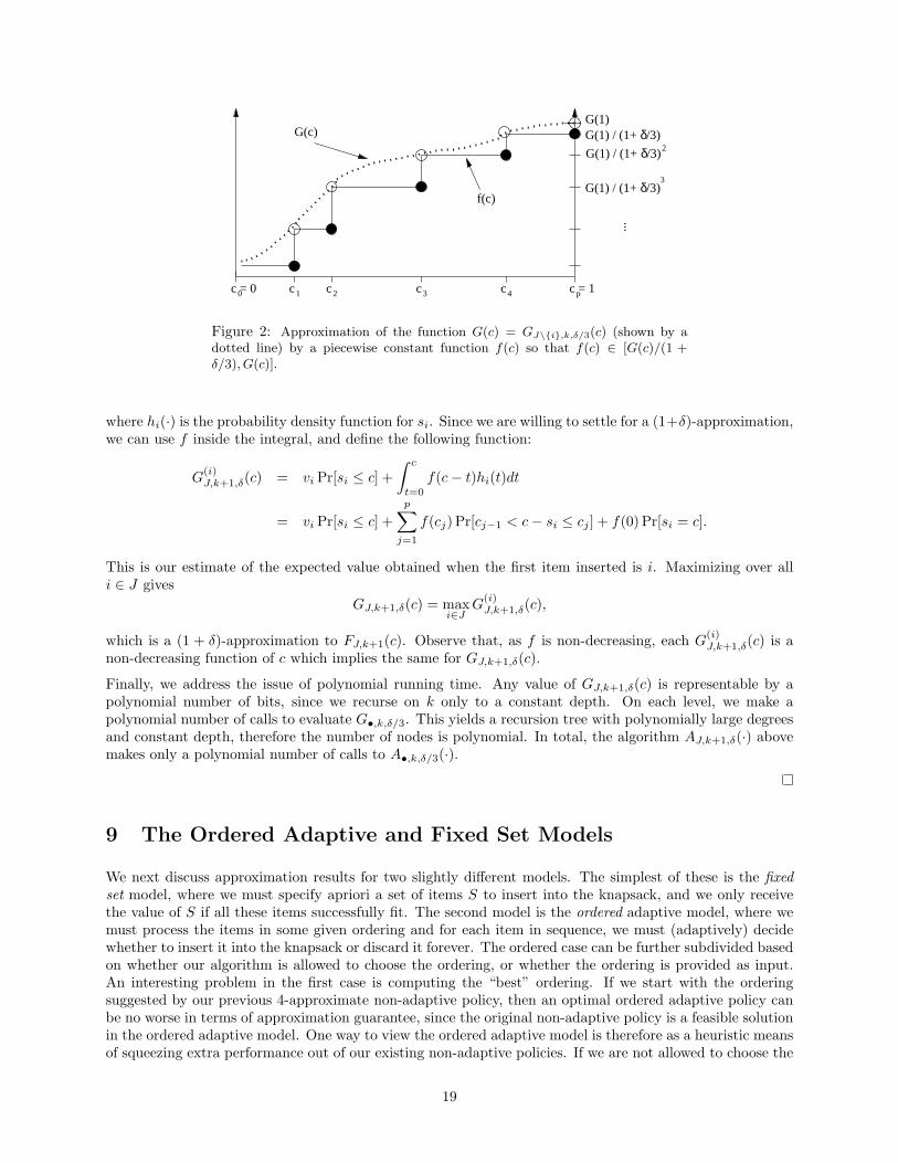
To remedy the problem above, we employ a sort of “assisted sampling” that first determines the interestingranges of values of si we should consider. For simplicity of notation, let us assume implied subscripts forthe moment and let G(c) denote GJ\{i},k,δ/3(c). We lower-bound G(·) by a piecewise constant functionf(·) with a polynomial number of breakpoints denoted 0 = c0, . . . , cp = 1. Our goal is to have f(·) be a(1 + δ)-approximation of F (·), so that we can use it to estimate the expected value of our near-optimalalgorithm. Initially we compute f(cp) = G(1)/(1 + δ/3) by a single invocation of AJ\{i},k,δ/3(1). We thenuse binary search to compute each successive breakpoint cp−1, . . . , c1 in reverse order. More precisely, oncewe have computed ci, we determine ci−1 to be the maximum value of c such that G(c) < f(ci) and we setf(ci−1) = G(ci−1)/(1 + δ/3). We illustrate the construction of f(·) in Figure 2. The maximum number ofsteps required by the binary search will be polynomial in n and b, since we will ensure (by induction to atmost a constant number of levels) that G(c) always evaluates to a quantity represented by polyk,δ(n, b) bits.

Each breakpoint of f(·) marks a change in G(·) by at least a (1 + δ/3) factor. This ensures that f will havepolyk,δ(n, b) breakpoints, since G always evaluates to a quantity represented by a polynomial number of bits.Since f is a (1 + δ/3)-approximation to G, which is in turn a (1 + δ/3)-approximation to FJ\{i},k, and since(1 + δ/3)2 ≤ 1 + δ, we know that f(c) ∈ [FJ\{i},k(c)/(1 + δ), FJ\{i},k(c)].

Assume for a moment now that i is the best first item to insert (the one that would be inserted first by anadaptive policy optimizing FJ,k+1(c), we can write FJ,k+1(c) as

FJ,k+1(c) = vi Pr[si ≤ c] +∫ c

t=0

FJ\{i},k(c− t)hi(t)dt.

18

G(c)

c1 c2 c3 c4

δ

δδ

pc = 1

2

3

...

f(c)

G(1)G(1) / (1+ /3)

G(1) / (1+ /3)

G(1) / (1+ /3)

0c = 0

Figure 2: Approximation of the function G(c) = GJ\{i},k,δ/3(c) (shown by adotted line) by a piecewise constant function f(c) so that f(c) ∈ [G(c)/(1 +δ/3), G(c)].

where hi(·) is the probability density function for si. Since we are willing to settle for a (1+δ)-approximation,we can use f inside the integral, and define the following function:

G(i)J,k+1,δ(c) = vi Pr[si ≤ c] +

∫ c

t=0

f(c− t)hi(t)dt

= vi Pr[si ≤ c] +p∑

j=1

f(cj) Pr[cj−1 < c− si ≤ cj ] + f(0) Pr[si = c].

This is our estimate of the expected value obtained when the first item inserted is i. Maximizing over alli ∈ J gives

GJ,k+1,δ(c) = maxi∈J

G(i)J,k+1,δ(c),

which is a (1 + δ)-approximation to FJ,k+1(c). Observe that, as f is non-decreasing, each G(i)J,k+1,δ(c) is a

non-decreasing function of c which implies the same for GJ,k+1,δ(c).

Finally, we address the issue of polynomial running time. Any value of GJ,k+1,δ(c) is representable by apolynomial number of bits, since we recurse on k only to a constant depth. On each level, we make apolynomial number of calls to evaluate G•,k,δ/3. This yields a recursion tree with polynomially large degreesand constant depth, therefore the number of nodes is polynomial. In total, the algorithm AJ,k+1,δ(·) abovemakes only a polynomial number of calls to A•,k,δ/3(·).

9 The Ordered Adaptive and Fixed Set Models

We next discuss approximation results for two slightly different models. The simplest of these is the fixedset model, where we must specify apriori a set of items S to insert into the knapsack, and we only receivethe value of S if all these items successfully fit. The second model is the ordered adaptive model, where wemust process the items in some given ordering and for each item in sequence, we must (adaptively) decidewhether to insert it into the knapsack or discard it forever. The ordered case can be further subdivided basedon whether our algorithm is allowed to choose the ordering, or whether the ordering is provided as input.An interesting problem in the first case is computing the “best” ordering. If we start with the orderingsuggested by our previous 4-approximate non-adaptive policy, then an optimal ordered adaptive policy canbe no worse in terms of approximation guarantee, since the original non-adaptive policy is a feasible solutionin the ordered adaptive model. One way to view the ordered adaptive model is therefore as a heuristic meansof squeezing extra performance out of our existing non-adaptive policies. If we are not allowed to choose the

19

ordering of items, an optimal ordered adaptive policy must at least be as good as an optimal solution in thefixed set model, since it is a feasible ordered adaptive policy to simply insert items in a fixed set, discardingall others (it is likely that the ordered adaptive policy will obtain more value than we would get in the fixedset model, since it gets “partial credit” even if only some of the items manage to fit). The main result weprove below is an approximation algorithm for the fixed set model that delivers a solution of expected valueFIXED ≥ (1/9.5)ADAPT . Therefore, the expected value obtained by an optimal ordered adaptive policyusing any initial ordering of items must fall within a factor of 9.5 of ADAPT .

Ordered adaptive models are worthwhile to consider because for a given ordering of items, we can computean optimal ordered adaptive policy in pseudo-polynomial time using dynamic programming (DP), as longas all item size distributions are discrete. By “discrete”, we mean that for some δ > 0, the support of si’sdistribution lies in {0, δ, 2δ, 3δ, . . .} for all items i. If the si’s are deterministic, then it is well known that anoptimal solution to the knapsack problem can be computed in O(n/δ) time via a simple dynamic program.The natural generalization of this dynamic program to the stochastic case gives us an O(n

δ log n) algorithmfor computing an optimal ordered policy. Let V (j, k) denote the optimal expected value one can obtain viaan ordered adaptive policy using only items j . . . n with kδ units of capacity left. Then

V (j, k) = max

{V (j + 1, k), vj Pr[sj ≤ kδ] +

k∑t=0

V (j + 1, k − t) Pr[sj = tδ]

}.

A straightforward DP implementation based on this recurrence runs in O(n2/δ) time, but we can speed thisup to O(n

δ log n) by using the Fast Fourier Transform to handle the convolution work for each row V (j, ·) inour table of subproblem solutions. An optimal adaptive solution in implicitly represented in the “traceback”paths through the table of subproblem solutions.

Although DP only applies to problems with discrete size distributions and only gives us pseudo-polynomialrunning times, we can discretize any set of size distributions in a manner that gives us a polynomial runningtime, at the expense of only a slight loss in terms of feasibility — our policy may overrun the capacity ofthe knapsack by a (1 + ε) factor, for a small constant ε > 0 of our choosing. Suppose we discretize thedistribution of si into a new distribution s′i with δ = ε/n (so s′i is represented by a vector of length n/ε),such that Pr[s′i = kδ] := Pr[kδ ≤ si < (k + 1)δ]. That is, we “round down” the probability mass in si tothe next-lowest multiple of δ. Since the “actual” size of each item (according to si) may be up to ε/n largerthan its “perceived” size (according to s′i), our policy may insert up to (1 + ε) units of mass before it thinksit has reached a capacity of 1.

9.1 An Approximation Algorithm for the Fixed Set Model

We now consider the computation of a set of items whose value times probability of fitting is at leastADAPT/9.5. Letting S denote the small items (µi ≤ ε) in our instance, we define

• m1 = maxi wi = maxi{vi Pr[si ≤ 1]}, and

• m2 = max{val(J)(1− µ(J)) : J ⊆ S}.

Note that m1 can be determined easily and m2 can be approximated to within any relative error by runningthe standard knapsack approximation scheme with mean sizes. Both values correspond to the expectedbenefit of inserting either a single item i or a set J of small items, counting only the event that the entireset fits in the knapsack. Our fixed set of items is the better of the two: FIXED = max{m1,m2}. We nowcompare ADAPT to FIXED.

Lemma 7. For any set J ⊆ S of small items,

val(J) ≤(

1 +4µ(J)1− ε2

)m2.

20

Proof. We proceed by induction on |J |. For J = ∅, the statement is trivial. If µ(J) ≥ (1 − ε)/2, choose aminimal K ⊆ J , such that µ(K) ≥ (1− ε)/2. Since the items have mean size at most ε, µ(K) cannot exceed(1 + ε)/2. By induction,

val(J \K) ≤(

1 +4(µ(J)− µ(K))

1− ε2

)m2

and since m2 ≥ val(K)(1 − µ(K)), for µ(K) ∈ [ 1−ε2 , 1+ε

2 ] we have µ(K)m2 ≥ val(K)µ(K)(1 − µ(K)) ≥14 (1− ε2)val(K), and val(J) = val(J \K) + val(K) ≤

(1 + 4µ(J)

1−ε2

)m2. Finally, if µ(J) < (1− ε)/2, then it

easily follows that val(J) ≤ m21−µ(J) ≤ (1 + 4µ(J)

1−ε2 ) m2.

Theorem 7. We have ADAPT ≤ 9.5 FIXED.

Proof. Fix an optimal adaptive policy P and let J = JS ∪ JL denote the (random) set of items that Pattempts to insert into the knapsack, partitioned into small and large items. For any large item i, letxi = Pr[i ∈ JL]. Then the expected value P obtains from large items is bounded by

∑i∈L xiwi. It follows

that

ADAPT ≤ E[val(JS)] +∑i∈L

xiwi

≤(

1 +4E[µ(JS)]

1− ε2

)m2 +

(∑i∈L

xi

)m1

=(

1 +4E[µ(JS)]

1− ε2

)m2 + E[|JL|]m1

≤(

1 +4E[µ(JS)]

1− ε2

)m2 +

E[µ(JL)]ε

m1

≤(

1 +4E[µ(JS)]

1− ε2+

E[µ(JL)]ε

)FIXED

≤(

1 + max(

41− ε2

,1ε

)E[µ(JS ∪ JL)]

)FIXED

≤(

1 + 2 max(

41− ε2

,1ε

))FIXED

and for ε =√

5 − 2 ≈ 0.236 this gives us ADAPT ≤ 9.48 FIXED. Recall that we do not know how tocompute m2 exactly in polynomial time, although we can approximate this quantity to within an arbitraryconstant factor. Taking this factor to be small enough, we obtain a 9.5-approximation algorithm that runsin polynomial time.

10 Conclusion

In this paper, we have developed tools for analyzing adaptive and non-adaptive strategies and their relativemerit for a basic stochastic knapsack problem. Extensions to more complex problems, such as packing,covering and scheduling problems, as well as slightly different stochastic models can be found in the Ph.D.theses of two of the authors [4, 27].

Acknowledgements. We would like to thank the anonymous referees for many useful suggestions. Thisresearch was supported in part by NSF grants CCR-0098018, ITR-0121495 and CCF-0515221, and ONRgrant N00014-05-1-0148. A preliminary version of this paper with somewhat weaker results appeared in [5].

21

A Appendix: Notes on the Polymatroid LP

Theorem 3 gives an upper bound of Ψ(2) on the adaptive optimum, where Ψ(t) is defined by a linear programin the following form:

Ψ(t) = max

{∑i

wixi :∀J ⊆ [n];

∑i∈J

µixi ≤ t(1−∏i∈J

(1− µi))

∀i ∈ [n]; xi ∈ [0, 1]

}.

Here we show that although this LP has an exponential number of constraints, it can be solved efficiently.In fact, the optimal solution can be written in a closed form. The important observation here is thatf(J) = 1 −

∏j∈J(1 − µj) is a submodular function. This can be seen for example by interpreting f(J) as

Pr[⋃

j∈J Ej ] where Ej are independent events occurring with probabilities µj . Such a function is submodularfor any collection of events, since for any K ⊂ J , we have

f(J ∪ {x})− f(J) = Pr[Ex \⋃j∈J

Ej ] ≤ Pr[Ex \⋃

j∈K

Ej ] = f(K ∪ {x})− f(K).

From now on, we assume that µi > 0 for each item, since items with µi = 0 can be inserted for free - inan optimal solution, they will be always present with xi = 1 and this only increases the value of Ψ(t) by aconstant. So assume µi > 0 and substitute zi = µixi. Then Ψ(t) can be written as

Ψ(t) = max

{∑i

wi

µizi :

∀J ⊆ [n]; z(J) ≤ tf(J)∀i ∈ [n]; zi ∈ [0, µi]

}

where f(J) is a submodular function. Naturally, tf(J) is submodular as well, for any t ≥ 0. For now, ignorethe constraints zi ≤ µi and define

Ψ(t) = max

{∑i

wi

µizi :

∀J ⊆ [n]; z(J) ≤ tf(J)∀i ∈ [n]; zi ≥ 0

}.

Observe that for t ≤ 1, we have Ψ(t) = Ψ(t), since zi ≤ µi is implied by the condition for J = {i}. However,now we can describe the optimal solution defining Ψ(t) explicitly.

As before, we assume that w1µ1

≥ w2µ2

≥ . . .. The linear program defining Ψ(t) is a polymatroid with rankfunction tf(J). The optimal solution can be found by a greedy algorithm which essentially sets the values ofz1, z2, z3, . . . successively as large as possible, without violating the constraints

∑ki=1 zi ≤ tf({1, 2, . . . , k}).

The solution is z1 = tµ1, z2 = tµ2(1− µ1), etc.:

zk = tf({1, 2, . . . , k})− tf({1, 2, . . . , k − 1}) = tµk

k−1∏i=1

(1− µi)

and submodularity guarantees that this in fact satisfies the constraints for all subsets J [21]. Thus we havea closed form for Ψ(t):

Ψ(t) = t

n∑k=1

wk

k−1∏i=1

(1− µi)

which yields in particular the formula for Ψ(1) = Ψ(1) that we mentioned at the end of Section 5.

Our original LP is an intersection of a polymatroid LP with a box; this is a polymatroid as well, see [21]. Itcan be described using a different submodular function g(J, t):

Ψ(t) = max

{∑i

wi

µizi :

∀J ⊆ [n]; z(J) ≤ g(J, t)∀i ∈ [n]; zi ≥ 0

}.

22

Note that the constraints zi ≤ µi are removed now. In general, the function g(J, t) can be obtained as

g(J, t) = minA⊆J

(tf(A) + µ(J \A))

(see [21]). Here, we get an even simpler form; we claim that it’s enough to take the minimum over A ∈ {∅, J}.Indeed, suppose the minimum is attained for a proper subset ∅ 6= M ⊂ J . Recall that we assume µi > 0 forall items. Choose x ∈ M , y ∈ J \M and let M1 = M \ {x}, M2 = M ∪ {y}. We have

f(M) = 1−∏i∈M

(1− µi) = 1− (1− µx)∏

i∈M1

(1− µi) = f(M1) + µx

∏i∈M1

(1− µi)

and similarlyf(M2) = 1−

∏i∈M2

(1− µi) = f(M) + µy

∏i∈M

(1− µi).

Now we distinguish two cases: If t∏

i∈M (1− µi) < 1 then

tf(M2) + µ(J \M2) = tf(M) + µyt∏i∈M

(1− µi) + µ(J \M)− µy < tf(M) + µ(J \M).

In case t∏

i∈M (1− µi) ≥ 1, we have t∏

i∈M1(1− µi) > 1:

tf(M) + µ(J \M) = tf(M1) + µxt∏

i∈M1

(1− µi) + µ(J \M1)− µx > tf(M1) + µ(J \M1).

Both cases contradict our assumption of minimality on M . Thus we have

g(J, t) = min{tf(J), µ(J)} = min

{t(1−

∏i∈J

(1− µi)),∑i∈J

µi

}.

Again, we can find the optimal solution for this polymatroid using the greedy algorithm:

zk = g({1, 2, . . . , k}, t)− g({1, 2, . . . , k − 1}, t)

= min

{t(1−

k∏i=1

(1− µi)),k∑

i=1

µi

}−min

{t(1−

k−1∏i=1

(1− µi)),k−1∑i=1

µi

}.

To further simplify, we can use the fact that f({1, 2, . . . , k}) = 1−∏k

i=1(1−µi) is “concave” as a function of∑ki=1 µi (when extended to a piecewise linear function f satisfying f(

∑ki=1 µi) = f({1, 2, . . . , k})). Therefore

there is at most one breaking point.

Define b to be the maximum k ≤ n such that

t(1−k∏

i=1

(1− µi)) ≥k∑

i=1

µi.

This certainly holds for k = 0 and due to concavity, it holds exactly up to k = b. Therefore

• For 0 ≤ k ≤ b: g({1, . . . , k}, t) =∑k

i=1 µi.

• For b < k ≤ n: g({1, . . . , k}, t) = t(1−∏b

i=1(1− µi)).

For the optimal LP solution, we get

• For 1 ≤ k ≤ b: zk = µk.

• For k = b + 1: zb+1 = t(1−∏b+1

i=1 (1− µi))−∑b

i=1 µi.

23

• For b + 2 ≤ k ≤ n: zk = tµk

∏k−1i=1 (1− µi).

The value of the optimal solution is

Ψ(t) =n∑

i=1

wi

µizi =

b∑k=1

wk +wb+1

µb+1

(t(1−

b+1∏i=1

(1− µi))−b∑

i=1

µi

)+ t

n∑k=b+2

wk

k−1∏i=1

(1− µi).

(where some of the terms might be void if b = 0, n− 1 or n). Thus we have the solution of Ψ(t) in a closedform. In some cases, it can be stronger than the formula presented in Corollary 1. Nonetheless, we knowthat both of them can differ from the actual optimum by a factor of 4.

References

[1] J.R. Birge and F.V. Louveaux, Introduction to stochastic programming, Springer Verlag, 1997.

[2] R.L. Carraway, R.L.Schmidt, and L.R. Weatherford, An algorithm for maximizing target achievementin the stochastic knapsack problem with normal returns, Naval Research Logistics 40 (1993), 161–173.

[3] C.-S. Chang, X. Chao, M. Pinedo, and R.R. Weber, On the optimality of LEPT and cµ rules formachines in parallel, Journal of Applied Probability 29 (1992), 667–681.

[4] B.C. Dean, Approximation algorithms for stochastic scheduling problems, Ph.D. thesis, MassachusettsInstitute of Technology, 2005.

[5] B.C. Dean, M.X. Goemans, and J. Vondrak, Approximating the stochastic knapsack problem: the benefitof adaptivity, Proceedings of the IEEE Symposium on Foundations of Computer Science (FOCS), 2004,pp. 208–217.

[6] C. Derman, C.J. Lieberman, and S.M. Ross, A renewal decision problem, Management Science 24(1978), no. 5, 554–561.

[7] H. Emmons and M. Pinedo, Scheduling stochastic jobs with due dates on parallel machines, EuropeanJournal of Operations Research 47 (1990), 49–55.

[8] U. Feige, On the sum of independent random variables with unbounded variance, and estimating theaverage degree in a graph, STOC, 2004, pp. 594–603.

[9] A. Goel and P. Indyk, Stochastic load balancing and related problems, FOCS, 1999, pp. 579–586.

[10] R.L. Graham, E.L. Lawler, J.K. Lenstra, and A.H.G. Rinnooy Kan, Optimization and approximation indeterministic sequencing and scheduling: A survey, Annals of Discrete Mathematics 5 (1979), 287–326.

[11] M. Henig, Risk criteria in a stochastic knapsack problem, Operations Research 38 (1990), no. 5, 820–825.

[12] N. Immorlica, D. Karger, M. Minkoff, and V. Mirrokni, On the costs and benefits of procrastination:Approximation algorithms for stochastic combinatorial optimization problems, SODA, 2004, pp. 184–693.

[13] J. Kleinberg, Y. Rabani, and E. Tardos, Allocating bandwidth for bursty connections, STOC, 1997,pp. 664–673.

[14] A. Kleywegt and J.D. Papastavrou, The dynamic and stochastic knapsack problem with random sizeditems, Operations Research 49 (2001), no. 1, 26–41.

[15] E. Koutsoupias and C.H. Papadimitriou, Beyond competitive analysis, SIAM Journal on Computing 30(2000), no. 1, 300–317.

[16] R.H. Mohring, A.S. Schulz, and M. Uetz, Approximation in stochastic scheduling: the power of LP-basedpriority policies, J. of the ACM 46 (1999), no. 6, 924–942.

24

[17] J.D. Papastavrou, S. Rajagopalan, and A. Kleywegt, The dynamic and stochastic knapsack problemwith deadlines, Management Science 42 (1996), no. 12, 1706–1718.

[18] M. Pinedo, Stochastic scheduling with release dates and due dates, Operations Reesearch 31 (1983),559–572.

[19] R. Ravi and A. Sinha, Hedging uncertainty: Approximation algorithms for stochastic optimization prob-lems, IPCO, 2004, pp. 101–115.

[20] M. Rothkopf, Scheduling with random service times, Management Science 12 (1966), no. 9, 707–713.

[21] A. Schrijver, Combinatorial optimization - polyhedra and efficiency, Springer Verlag, 2003.

[22] D.B. Shmoys and C. Swamy, Stochastic optimization is (almost) as easy as deterministic optimization,FOCS, 2004, pp. 228–237.

[23] M. Skutella and M. Uetz, Stochastic machine scheduling with precedence constraints, To appear in theSIAM Journal on Computing.

[24] M. Sniedovich, Preference order stochastic knapsack problems: methodological issues, The Journal ofthe Operational Research Society 31 (1980), no. 11, 1025–1032.

[25] E. Steinberg and M.S. Parks, A preference order dynamic program for a knapsack problem with stochasticrewards, The Journal of the Operational Research Society 30 (1979), no. 2, 141–147.

[26] M. Uetz, Algorithms for deterministic and stochastic scheduling, Ph.D. thesis, Institut fur Mathematik,Technische Universitat Berlin, 2001.

[27] J. Vondrak, Probabilistic methods in combinatorial and stochastic optimization, Ph.D. thesis, Mas-sachusetts Institute of Technology, 2005.

25