Approximating the Minimum Spanning Tree Weight in Sublinear Time Speaker: Chuang-Chieh Lin Advisor:...
85
Approximating the Minimum Spanning Tree Weight in Sublinear Time Speaker: Chuang-Chieh Lin Advisor: Professor Maw-Shang Chang Computation Theory Laboratory National Chung Cheng University Bernard Chazelle, Ronitt Rubinfeld and Luca Trevisan SIAM Journal on Computing, Vol. 34, No. 6, July, 2005, pp. 1370-1379.
-
Upload
baldwin-young -
Category
Documents
-
view
222 -
download
0
Transcript of Approximating the Minimum Spanning Tree Weight in Sublinear Time Speaker: Chuang-Chieh Lin Advisor:...

Approximating the Minimum Spanning Tree Weight in Sublinear
Time
Speaker: Chuang-Chieh LinAdvisor: Professor Maw-Shang Chang
Computation Theory LaboratoryNational Chung Cheng University
Bernard Chazelle, Ronitt Rubinfeld and Luca Trevisan
SIAM Journal on Computing, Vol. 34, No. 6, July, 2005, pp. 1370-1379.

Computation Theory Lab., Dept. CSIE, CCU, TaiwanComputation Theory Lab., Dept. CSIE, CCU, Taiwan2
Bernard Chazelle, Department of Computer Science, Princeton University
Department of Electrical Engineering and Computer Science, MIT
Computer Science Division, University of California-Berkeley

Computation Theory Lab., Dept. CSIE, CCU, TaiwanComputation Theory Lab., Dept. CSIE, CCU, Taiwan3
Outline
• Introduction• Related works• An overview of the algorithm in this paper• Approximating the average degree• Estimating the number of connected components• Approximating the weight of an MST• Conclusions
Computation Theory Lab., Dept. CSIE, CCU, TaiwanComputation Theory Lab., Dept. CSIE, CCU, Taiwan4
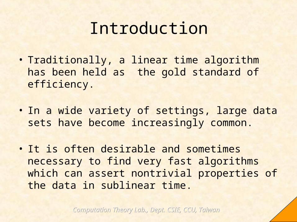
Introduction
• Traditionally, a linear time algorithm has been held as the gold standard of efficiency.
• In a wide variety of settings, large data sets have become increasingly common.
• It is often desirable and sometimes necessary to find very fast algorithms which can assert nontrivial properties of the data in sublinear time.

Computation Theory Lab., Dept. CSIE, CCU, TaiwanComputation Theory Lab., Dept. CSIE, CCU, Taiwan5
Introduction (contd.)
• One direction of research that has been suggested is that of property testing. [RS96, GG98]
• Property testing algorithms distinguish between inputs that have a certain property and those are far from having the property.
• Property testing can be viewed as a natural type of approximation problem.

Computation Theory Lab., Dept. CSIE, CCU, TaiwanComputation Theory Lab., Dept. CSIE, CCU, Taiwan6
Introduction (contd.)
• Many of the property testers have led to very fast, even constant time, approximation schemes for associated problem. [GG98, FK99, FKV04, ADPR03]
• For example, one can approximate the value of a maximum cut in a dense graph in time , with relative error at most , by looking at only O( –7
log 1/) locations in the adjacency matrix. [GG98]
)/1log( 3
2 O

Computation Theory Lab., Dept. CSIE, CCU, TaiwanComputation Theory Lab., Dept. CSIE, CCU, Taiwan7
Outline
• Introduction• Related works• An overview of the algorithm in this paper• Approximating the average degree• Estimating the number of connected components• Approximating the weight of an MST• Conclusions

Computation Theory Lab., Dept. CSIE, CCU, TaiwanComputation Theory Lab., Dept. CSIE, CCU, Taiwan8
Related works
• Finding the minimum spanning tree (MST) of a graph has a long, distinguished history [C00b, GH85, N97].
• Currently the best known deterministic algorithm was proposed by Chazelle [C00a].
• Chazelle’s algorithm runs in O(mα(m, n)) time, where n (resp., m) is the number of vertices (resp., edges) and αis inverse-Ackermann.

Computation Theory Lab., Dept. CSIE, CCU, TaiwanComputation Theory Lab., Dept. CSIE, CCU, Taiwan9
Related works (contd.)
• Karger, Klein and Tarjan [KKT95] gave a randomized algorithm which runs in linear expected time.
• In this paper, we consider the problem of finding the weight of the minimum spanning tree (MST) of a graph.
• There are conditions under which it is possible to approximate the weight of the MST of a connected graph in sublinear time in the number of edges.

Computation Theory Lab., Dept. CSIE, CCU, TaiwanComputation Theory Lab., Dept. CSIE, CCU, Taiwan10
Outline
• Introduction• Related works• An overview of the algorithm in this paper• Approximating the average degree• Estimating the number of connected components• Approximating the weight of an MST• Conclusions
Computation Theory Lab., Dept. CSIE, CCU, TaiwanComputation Theory Lab., Dept. CSIE, CCU, Taiwan11
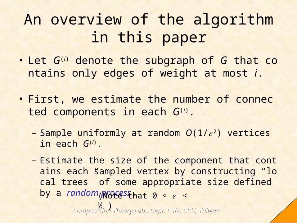
An overview of the algorithm in this paper
• Let G(i) denote the subgraph of G that contains only edges of weight at most i.
• First, we estimate the number of connected components in each G(i).
– Sample uniformly at random O(1/ 2) vertices in each G(i).
– Estimate the size of the component that contains each sampled vertex by constructing “local trees” of some appropriate size defined by a random process.
(Note that 0 < < ½ )

Computation Theory Lab., Dept. CSIE, CCU, TaiwanComputation Theory Lab., Dept. CSIE, CCU, Taiwan12
An overview of the algorithm in this paper (contd.)
• Second, we can in turn produce a good approximation for the weight of the MST of G.
• Estimating the number of connected components in a graph runs in time within an additive error of n of the true count.
– d is the average degree of the graph.
– We can ensure that d can be approximated in O(d/) expected time and that at most n/4 vertices having degree greater than the estimate of d.
)log( 2
ddO

Computation Theory Lab., Dept. CSIE, CCU, TaiwanComputation Theory Lab., Dept. CSIE, CCU, Taiwan13
An overview of the algorithm in this paper (contd.)
• The method for estimating the number of connected components in a graph is based on a similar principle as the property tester for graph connectivity given by Goldreich and Ron [GR02].
• The total running time is O(dw –2 log dw/). It does N
OT depend on the number of vertices in G.

Computation Theory Lab., Dept. CSIE, CCU, TaiwanComputation Theory Lab., Dept. CSIE, CCU, Taiwan14
Outline
• Introduction• Related works• An overview of the algorithm in this paper• Approximating the average degree• Estimating the number of connected components• Approximating the weight of an MST• Conclusions

Computation Theory Lab., Dept. CSIE, CCU, TaiwanComputation Theory Lab., Dept. CSIE, CCU, Taiwan15
Approximating the average degree
• Pick C/ vertices of G at random, for some large constant C and set d
* to be the maximum degree among them.
– To find the degree of any one of them takes O(d) time on average, so the expected running time is O(Cd/) = O(d/).
• (Imagine the vertex degrees sorted in nonincreasing order…☺) Let ρ be the rank of d
*.– With high probability, ρ=Θ( n)
– Why?

Computation Theory Lab., Dept. CSIE, CCU, TaiwanComputation Theory Lab., Dept. CSIE, CCU, Taiwan16
Approximating the average degree (contd.)
• Pr({ρ > n}) = (1– )C/ ≤ e–C
– Since (1 + )1/ e, when 0.
• Pr({ρ > n/C2}) = (1– /C2)C/
≥ e–2/C (…☺…) > 1 – 2/C.
– Try to prove that f (x) = x + e –x > 1
0
1
ρ
/C2
In my opinion, we can assume that C ≥ 1.

Computation Theory Lab., Dept. CSIE, CCU, TaiwanComputation Theory Lab., Dept. CSIE, CCU, Taiwan17
Approximating the average degree (contd.)
• Lemma 1: In O(d/) expected time, we can compute a vertex degree d
* that, with high probability, is the kth largest vertex degree for some k =Θ( n).
– Note: k = Ω( n) alone implies that d * = O(d/).– Why?

Computation Theory Lab., Dept. CSIE, CCU, TaiwanComputation Theory Lab., Dept. CSIE, CCU, Taiwan18
Approximating the average degree (contd.)
• By C. M. Lee:– Since k = Ω( n), we can assume that k ≥ q n for some posi
tive constant q.
– Consider the fact that kd *≤ ΣvV deg(v).
• Why?
•
• Thus d * = O(d/).
0
1
k
My weekly report…

Computation Theory Lab., Dept. CSIE, CCU, TaiwanComputation Theory Lab., Dept. CSIE, CCU, Taiwan19
Approximating the average degree (contd.)
• If we scale by the proper constant, we can ensure that at most n/4 vertices have degree higher than d
*.
Lemma 1: In O(d/) expected time, we can compute a vertex degree d
* that, with high probability, is the kth largest vertex degree for some k = ( n).
0
1
k

Computation Theory Lab., Dept. CSIE, CCU, TaiwanComputation Theory Lab., Dept. CSIE, CCU, Taiwan20
Outline
• Introduction• Related works• An overview of the algorithm in this paper• Approximating the average degree• Estimating the number of connected components• Approximating the weight of an MST• Conclusions

Computation Theory Lab., Dept. CSIE, CCU, TaiwanComputation Theory Lab., Dept. CSIE, CCU, Taiwan21
Other preliminaries and notations
• Let d denote the average degree of the graph.
• Edge weights are in the set {1, …, w}.
• Let c denote the number of connected components of the graph.
• The algorithm requires no prior information about the graph besides w and n. (n is the number of vertices)

Computation Theory Lab., Dept. CSIE, CCU, TaiwanComputation Theory Lab., Dept. CSIE, CCU, Taiwan22
Estimating the number of connected components
• Let du be the number of edges incident upon it (including self-loops).
• Let mu be the number of edges in u’s component in G.
• Consider the following fact.
FACT: Given a graph with vertex set V, for every component I V,
./2
1 and 1/
2
1cmdmd
Vuuu
Iuuu
This is concerned with a problem in the algorithm course ...Besides, we let du/mu = 2 for an isolated vertex u. (mu= 0 here)

Computation Theory Lab., Dept. CSIE, CCU, TaiwanComputation Theory Lab., Dept. CSIE, CCU, Taiwan23
• The algorithm is as follows:

Computation Theory Lab., Dept. CSIE, CCU, TaiwanComputation Theory Lab., Dept. CSIE, CCU, Taiwan24
approx-number-connected-components(G, , W,
d*)Uniformly choose r = O(1/
2) vertices u1,…,ur
For each vertex ui ,
Set βi = 0
Take the first step of a BFS from ui
(*) Flip a coin!!
If (heads) & (# vertices visited in BFS < W)
& (no visited vertex has degree > d *)
then { Resume BFS to double number of visited edges
If this allows BFS to complete
then { If mui = 0 set βi = 2;
else set βi = dui2#coin flips/#edges visited in BFS }
else go to (*) }
Output
r
i ir
nc
12ˆ
Visit the single vertex ui and all its dui incident edges
log(mui /dui
)At least 1?At least 1?

Computation Theory Lab., Dept. CSIE, CCU, TaiwanComputation Theory Lab., Dept. CSIE, CCU, Taiwan25
A
B C D
E F GA
Illustration 1 for BFS with coin flips
mA = 0dA = 0

Computation Theory Lab., Dept. CSIE, CCU, TaiwanComputation Theory Lab., Dept. CSIE, CCU, Taiwan26
A
B C D
E F GBCD
First step of a BFS from A
H
Resume BFS to double number of visited edges
mA = 3dA = 3

Computation Theory Lab., Dept. CSIE, CCU, TaiwanComputation Theory Lab., Dept. CSIE, CCU, Taiwan27
A
B C D
E F GCDEF
mA = 5dA = 3
Computation Theory Lab., Dept. CSIE, CCU, TaiwanComputation Theory Lab., Dept. CSIE, CCU, Taiwan28
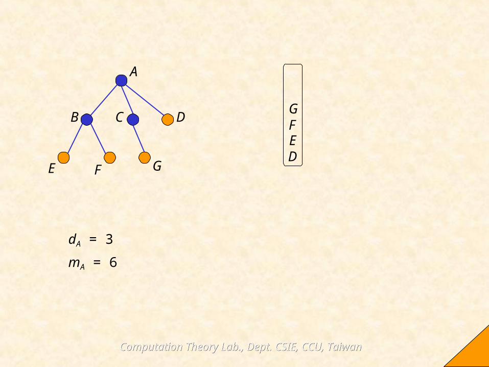
A
B C D
E F G
G
DEF
mA = 6dA = 3

Computation Theory Lab., Dept. CSIE, CCU, TaiwanComputation Theory Lab., Dept. CSIE, CCU, Taiwan29
A
B C D
E F G
G
EF
mA = 6dA = 3

Computation Theory Lab., Dept. CSIE, CCU, TaiwanComputation Theory Lab., Dept. CSIE, CCU, Taiwan30
A
B C D
E F G
GF
mA = 6dA = 3

Computation Theory Lab., Dept. CSIE, CCU, TaiwanComputation Theory Lab., Dept. CSIE, CCU, Taiwan31
A
B C D
E F GG
mA = 6dA = 3
Computation Theory Lab., Dept. CSIE, CCU, TaiwanComputation Theory Lab., Dept. CSIE, CCU, Taiwan32
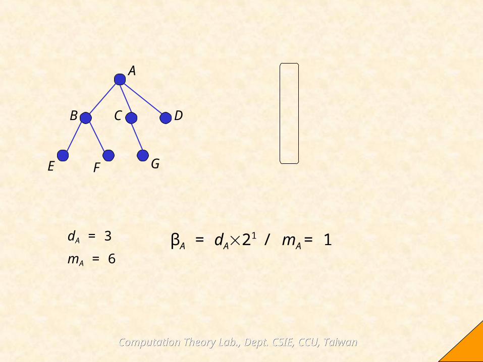
A
B C D
E F G
mA = 6dA = 3 βA = dA21 / mA = 1

Computation Theory Lab., Dept. CSIE, CCU, TaiwanComputation Theory Lab., Dept. CSIE, CCU, Taiwan33
A
B C D
A
Illustration 2 for BFS with coin flips
mA = 0dA = 0
E

Computation Theory Lab., Dept. CSIE, CCU, TaiwanComputation Theory Lab., Dept. CSIE, CCU, Taiwan34
A
B C D
BCD
First step of a BFS from A
H
Resume BFS to double number of visited edges
mA = 3dA = 3
E
Computation Theory Lab., Dept. CSIE, CCU, TaiwanComputation Theory Lab., Dept. CSIE, CCU, Taiwan35
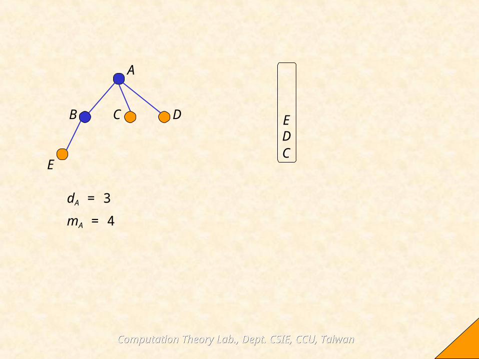
A
B C D
CD
mA = 4dA = 3
E
E

Computation Theory Lab., Dept. CSIE, CCU, TaiwanComputation Theory Lab., Dept. CSIE, CCU, Taiwan36
A
B C D
D
mA = 4dA = 3
E
E

Computation Theory Lab., Dept. CSIE, CCU, TaiwanComputation Theory Lab., Dept. CSIE, CCU, Taiwan37
A
B C D
mA = 4dA = 3
EE

Computation Theory Lab., Dept. CSIE, CCU, TaiwanComputation Theory Lab., Dept. CSIE, CCU, Taiwan38
A
B C D
βA = dA21 / mA = 1.5mA = 4dA = 3
E

Computation Theory Lab., Dept. CSIE, CCU, TaiwanComputation Theory Lab., Dept. CSIE, CCU, Taiwan39
A
B
A
mA = 0dA = 0
Illustration 3 for BFS with coin flips
G
C D E F

Computation Theory Lab., Dept. CSIE, CCU, TaiwanComputation Theory Lab., Dept. CSIE, CCU, Taiwan40
B
First step of a BFS from A
H
Resume BFS to double number of visited edges
mA = 5dA = 5
C D E F
A
B
G
CDEF

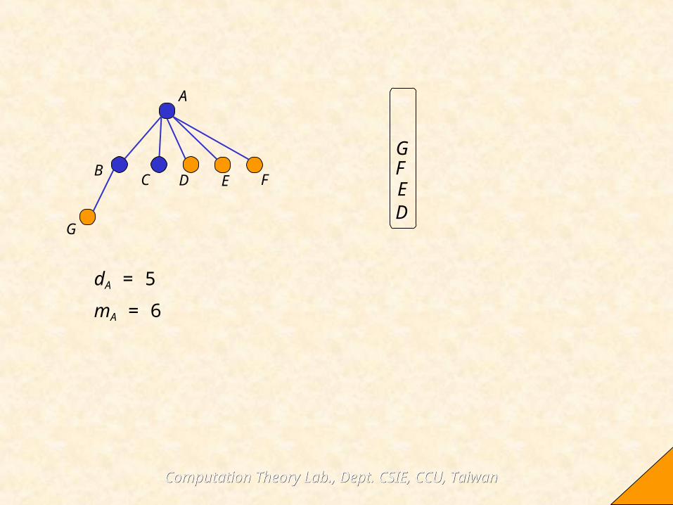
Computation Theory Lab., Dept. CSIE, CCU, TaiwanComputation Theory Lab., Dept. CSIE, CCU, Taiwan41
mA = 6dA = 5
C D E F
A
B
GCDEFG
Computation Theory Lab., Dept. CSIE, CCU, TaiwanComputation Theory Lab., Dept. CSIE, CCU, Taiwan42
mA = 6dA = 5
C D E F
A
B
GDEFG

Computation Theory Lab., Dept. CSIE, CCU, TaiwanComputation Theory Lab., Dept. CSIE, CCU, Taiwan43
mA = 6dA = 5
C D E F
A
B
GEFG

Computation Theory Lab., Dept. CSIE, CCU, TaiwanComputation Theory Lab., Dept. CSIE, CCU, Taiwan44
mA = 6dA = 5
C D E F
A
B
GFG

Computation Theory Lab., Dept. CSIE, CCU, TaiwanComputation Theory Lab., Dept. CSIE, CCU, Taiwan45
mA = 6dA = 5
C D E F
A
B
GG

Computation Theory Lab., Dept. CSIE, CCU, TaiwanComputation Theory Lab., Dept. CSIE, CCU, Taiwan46
mA = 6dA = 5
C D E F
A
B
G
βA = dA21 / mA = 5/3
Computation Theory Lab., Dept. CSIE, CCU, TaiwanComputation Theory Lab., Dept. CSIE, CCU, Taiwan47
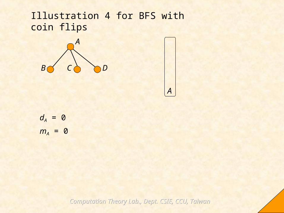
A
B C D
A
Illustration 4 for BFS with coin flips
mA = 0dA = 0
Computation Theory Lab., Dept. CSIE, CCU, TaiwanComputation Theory Lab., Dept. CSIE, CCU, Taiwan48
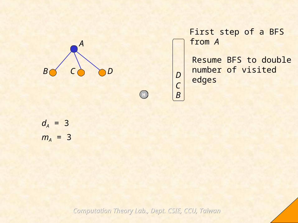
A
B C D
BCD
First step of a BFS from A
H
Resume BFS to double number of visited edges
mA = 3dA = 3

Computation Theory Lab., Dept. CSIE, CCU, TaiwanComputation Theory Lab., Dept. CSIE, CCU, Taiwan49
A
B C D
CD
mA = 3dA = 3

Computation Theory Lab., Dept. CSIE, CCU, TaiwanComputation Theory Lab., Dept. CSIE, CCU, Taiwan50
A
B C D
D
mA = 3dA = 3

Computation Theory Lab., Dept. CSIE, CCU, TaiwanComputation Theory Lab., Dept. CSIE, CCU, Taiwan51
A
B C D
mA = 3dA = 3

Computation Theory Lab., Dept. CSIE, CCU, TaiwanComputation Theory Lab., Dept. CSIE, CCU, Taiwan52
A
B C D
βA = dA21 / mA = 2mA = 3dA = 3

Computation Theory Lab., Dept. CSIE, CCU, TaiwanComputation Theory Lab., Dept. CSIE, CCU, Taiwan53
Estimating the number of connected components (contd.)
• Notice that W is a threshold value which is set to 4/ for counting connected components.
• Note that if the BFS from ui completes, the number of coin flips associated with it is log(mui
/dui) (at least 1).
– Think about it!

Computation Theory Lab., Dept. CSIE, CCU, TaiwanComputation Theory Lab., Dept. CSIE, CCU, Taiwan54
Estimating the number of connected components (contd.)
• Let S denote the set of vertices that lie in components with fewer than W vertices all of which are of degree at most d
*.
• If ui S, then βi is 2lg(mui /dui
)dui /mui
with probability 2–lg
(mui /dui
) (and 2 if mui = 0);
• If ui S, then βi = 0.1 ≤ βi ≤ 2

Computation Theory Lab., Dept. CSIE, CCU, TaiwanComputation Theory Lab., Dept. CSIE, CCU, Taiwan55
Estimating the number of connected components (contd.)
• Since βi ≤ 2, we have
.4
2
][2
][
][][var2
22
n
c
m
d
n
E
E
EE
Su u
u
i
i
iii
Vu u
u cm
d
2
1
Su u
u
Su u
u
m
d
n
m
d
Sn
S
1
||
1||
x
xfxXXE )(]Pr[][

Computation Theory Lab., Dept. CSIE, CCU, TaiwanComputation Theory Lab., Dept. CSIE, CCU, Taiwan56
Estimating the number of connected components (contd.)
• Thus the variance of ĉ is bounded by
.var4
)2
var(ˆvar2
2
r
ncr
r
n
r
nc i
ii

Computation Theory Lab., Dept. CSIE, CCU, TaiwanComputation Theory Lab., Dept. CSIE, CCU, Taiwan57
Estimating the number of connected components (contd.)
• By our choice of W = 4/ and d *, there are at most
n/2 components NOT in S, so:
.ˆ2
ccEn
c
The number of connected components in S.
Components: n/(4/) =
n/4
There are at most n/4 vertices having degree greater than d*

Computation Theory Lab., Dept. CSIE, CCU, TaiwanComputation Theory Lab., Dept. CSIE, CCU, Taiwan58
Estimating the number of connected components (contd.)
• Furthermore, by Chebyshev’s Inequality,
• Choosing r = O(1/ 2) ensures that, with constant
probability arbitrary close to 1, our estimate ĉ of the number of connected components deviates from the actual value by at most n.
.4
)2/(
ˆvar]
2|ˆˆPr[|
22 rn
c
n
cncEc
.4
1]|ˆˆ||ˆ||ˆPr[|2rn
cncEccEccc
Computation Theory Lab., Dept. CSIE, CCU, TaiwanComputation Theory Lab., Dept. CSIE, CCU, Taiwan59
Estimating the number of connected components (contd.)
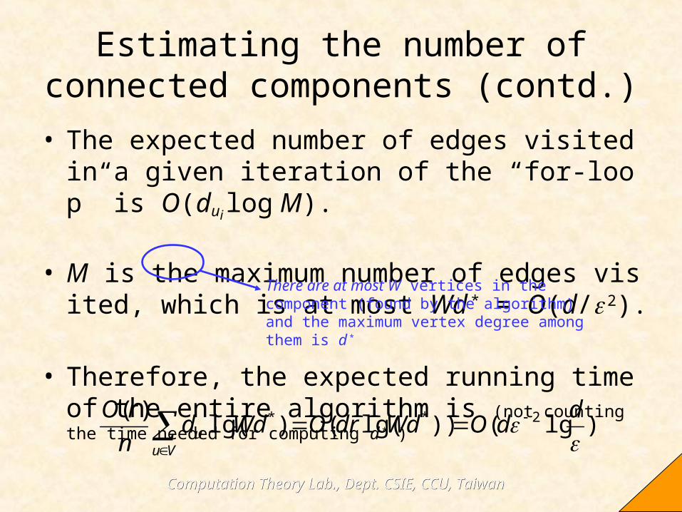
• The expected number of edges visited in a given iteration of the “for-loop” is O(dui log M).
• M is the maximum number of edges visited, which is at most Wd
* = O(d/ 2).
• Therefore, the expected running time of the entire algorithm is (not counting the time needed for computing d
* )
There are at most W vertices in the component (found by the algorithm) and the maximum vertex degree among them is d
*
).lg())lg(()lg()( 2**
d
dOWddrOWddn
rO
Vuu
Computation Theory Lab., Dept. CSIE, CCU, TaiwanComputation Theory Lab., Dept. CSIE, CCU, Taiwan60
Estimating the number of connected components (contd.)
• The algorithm’s running time is randomized.
• However, if d is known, we can get a deterministic running time bounded by stopping the algorithm after Cd
–2 log(d/) steps and output 0 if the algorithm has no
t yet terminated.
• This event occurs with probability at most O(1/C).
• Therefore we obtain the following theorem.

Computation Theory Lab., Dept. CSIE, CCU, TaiwanComputation Theory Lab., Dept. CSIE, CCU, Taiwan61
Estimating the number of connected components (contd.)
• Theorem 1. Let c be the number of components in a graph with n vertices. Then Algorithm approx-number-connected-components runs in time O(d
–2 log d/) and with probability at least ¾ outputs ĉ such that |c – ĉ| ≤ n.

Computation Theory Lab., Dept. CSIE, CCU, TaiwanComputation Theory Lab., Dept. CSIE, CCU, Taiwan62
Estimating the number of connected components (contd.)
• Actually,
can be fine-tuned to be
.4
)2/(
ˆvar]
2|ˆˆPr[|
22 rn
c
n
cncEc
.constant enough large somefor ,8
]2
|~~Pr[| AA
ncEc
We omit the details here, OK?
Computation Theory Lab., Dept. CSIE, CCU, TaiwanComputation Theory Lab., Dept. CSIE, CCU, Taiwan63
Outline
• Introduction• Related works• An overview of the algorithm in this paper• Approximating the average degree• Estimating the number of connected components• Approximating the weight of an MST• Conclusions

Computation Theory Lab., Dept. CSIE, CCU, TaiwanComputation Theory Lab., Dept. CSIE, CCU, Taiwan64
Approximating the weight of an MST
• Now we are going to present an algorithm for approximating the value of the MST in bounded weight graphs.
• We are given a connected graph G with average degree d and with each edge assigned an integer weight between 1 and w.
• We assume that G is represented by adjacency lists.

Computation Theory Lab., Dept. CSIE, CCU, TaiwanComputation Theory Lab., Dept. CSIE, CCU, Taiwan65
Approximating the weight of an MST (contd.)
• Let G(p) be the subgraph of G consisting of all the edges of weight at most p.
• Let c(p) be the number of connected components in G(p).– Then what is c(0)? What is c(w) ?
• Let M(G) denote the weight of the MST of G.
0 ≤ p ≤ w
c(0) = n and c(w)= 1

Computation Theory Lab., Dept. CSIE, CCU, TaiwanComputation Theory Lab., Dept. CSIE, CCU, Taiwan66
Approximating the weight of an MST (contd.)
• Consider the case that G has only edges of weight 1 or 2 (i.e., w = 2).
• c(1) is the number of connected components in G(1).
• Then any MST of G must contain exactly c(1) – 1
edges of weight 2 (Why?) with the others being of weight 1.
• Thus the weight of the MST is exactly 2(c(1) – 1) + [(n
– 1) – (c(1) – 1)] 1 = n – 2 + c(1).

Computation Theory Lab., Dept. CSIE, CCU, TaiwanComputation Theory Lab., Dept. CSIE, CCU, Taiwan67
Approximating the weight of an MST (contd.)
• Then we can generalize the previous derivation to any w.
• CLAIM: For integer w ≥ 2,
.)(1
1
)(
w
i
icwnGM

Computation Theory Lab., Dept. CSIE, CCU, TaiwanComputation Theory Lab., Dept. CSIE, CCU, Taiwan68
Approximating the weight of an MST (contd.)
• Proof of the CLAIM:– Let αi be the number of edges of weight i in an MST of G.
• Note that αi is independent of which MST we choose. [G68]
– For all 0 ≤ p ≤ w – 1,
– Therefore,
.1)( pi
pi c
.
1)(
1
1
)(1
0
)(
1
0
)(1
0 11
w
i
iw
p
p
w
p
pw
p
w
pii
w
ii
cwncw
ciGM

Computation Theory Lab., Dept. CSIE, CCU, TaiwanComputation Theory Lab., Dept. CSIE, CCU, Taiwan69
Approximating the weight of an MST (contd.)
• Therefore, we can find that computing the number of connected components allows us to compute the weight of the MST of G.
Computation Theory Lab., Dept. CSIE, CCU, TaiwanComputation Theory Lab., Dept. CSIE, CCU, Taiwan70
Approximating the weight of an MST (contd.)
• Now let us proceed with the main algorithm approximating the value of the MST.
• It approximates the value of the MST by estimating each of the c(p)’s.
• Due to the analysis of the complexity, W is set to 4w/ here, not 4/.
(Imagine that is substituted to be
/w)

Computation Theory Lab., Dept. CSIE, CCU, TaiwanComputation Theory Lab., Dept. CSIE, CCU, Taiwan71
Approximating the weight of an MST (contd.)
• For the same reason, we need a different estimate of d *.
– In O(dw/) time, an estimate d * = O(dw/) such that at most
n/4w vertices have degree higher than d *.
Computation Theory Lab., Dept. CSIE, CCU, TaiwanComputation Theory Lab., Dept. CSIE, CCU, Taiwan72
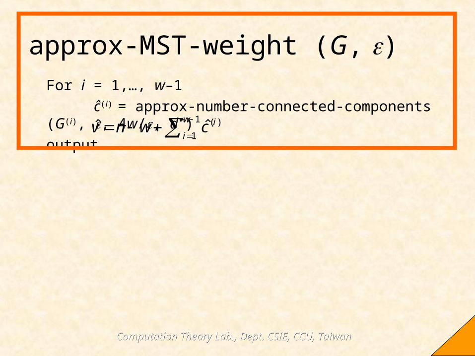
approx-MST-weight (G, )For i = 1,…, w–1
ĉ(i) = approx-number-connected-components(G(i), , 4w/, d *)
output
1
1
)(ˆˆw
i
icwnv

Computation Theory Lab., Dept. CSIE, CCU, TaiwanComputation Theory Lab., Dept. CSIE, CCU, Taiwan73
Approximating the weight of an MST (contd.)
• Theorem 2. Let w/n < ½. Let v be the weight of the MST of G. Algorithm approx-MST-weight (G, ) runs in time O(dw
–2 log dw/) and outputs a value that, with high probability at least ¾ , differs from v by at most n.
v̂
We have to show that
.|ˆ| vvv
Computation Theory Lab., Dept. CSIE, CCU, TaiwanComputation Theory Lab., Dept. CSIE, CCU, Taiwan74
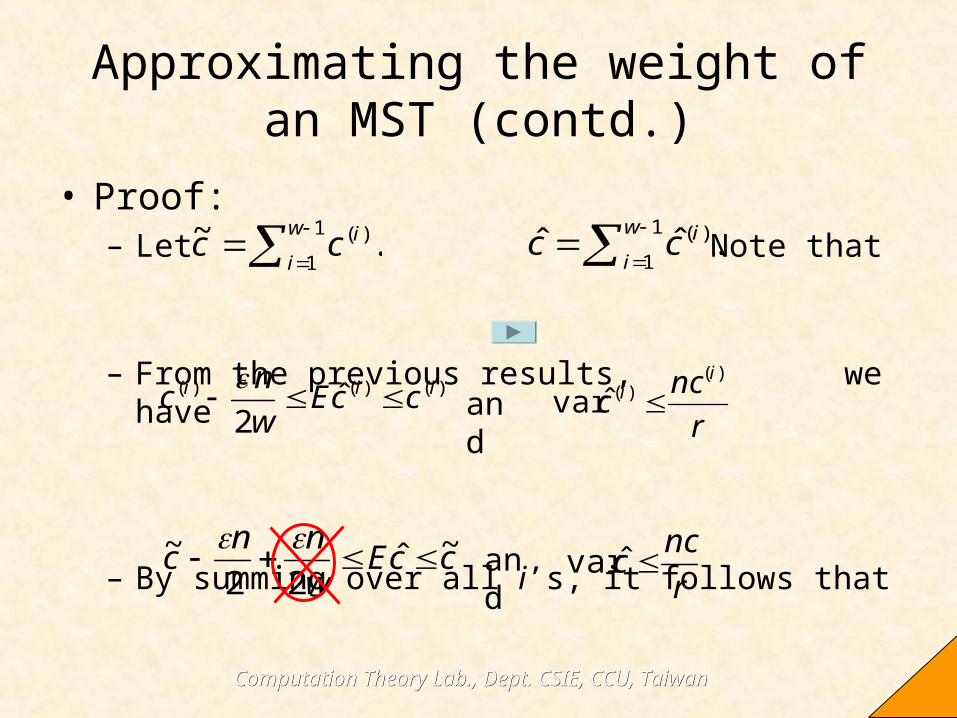
Approximating the weight of an MST (contd.)
• Proof:– Let Note that
– From the previous results, we have
– By summing over all i’s, it follows that
)()()( ˆ2
iii ccEw
nc
and
r
ncc
ii
)()(ˆvar
ccEw
nnc ~ˆ
22~
and
r
ncc ˆvar
.~ 1
1
)(
w
i
icc .ˆˆ1
1
)(
w
i
icc

Computation Theory Lab., Dept. CSIE, CCU, TaiwanComputation Theory Lab., Dept. CSIE, CCU, Taiwan75
Dear Chuang-Chieh
Thanks for your interest in the article.I think we're both correct.
You say:"By summing over $i$, it follows that $\sum_{i=1}^{w-1}c^{(i)} -(w-1)(\epsilon n/2w) = c-\epsilon n/2 + \epsilon n/2w \leq E\hat{c}\leqc$ and ...."
which is true.
but this implies that
c- \epsilon n/2 \leq E\hat{c}
which is what we write. In other words, we simply leave outthe intermediate step to make the math shorter.but it's still entirely correct.
Hope this helps.
Bernard Chazelle

Computation Theory Lab., Dept. CSIE, CCU, TaiwanComputation Theory Lab., Dept. CSIE, CCU, Taiwan76
Approximating the weight of an MST (contd.)
• Choosing r 2 large enough, by Chebyshev’s
Inequality, we have
which can be arbitrary small.
• Then with high probability,
22 )~(
~9]
3
)~(|ˆˆPr[|
cwnr
cncwncEc
.3
)~(
2|ˆ~||ˆ| v
cwnnccvv
v
= v ≥ n – 1

Computation Theory Lab., Dept. CSIE, CCU, TaiwanComputation Theory Lab., Dept. CSIE, CCU, Taiwan77
Approximating the weight of an MST (contd.)
• Time complexity?
• Each call to approx-number-connected-components is O(d
–2 log dw/).
• Therefore the total expected running time is O(dw
–2 log dw/).

Computation Theory Lab., Dept. CSIE, CCU, TaiwanComputation Theory Lab., Dept. CSIE, CCU, Taiwan78
Outline
• Introduction• Related works• An overview of the algorithm in this paper• Approximating the average degree• Estimating the number of connected components• Approximating the weight of an MST• Conclusions

Computation Theory Lab., Dept. CSIE, CCU, TaiwanComputation Theory Lab., Dept. CSIE, CCU, Taiwan79
Conclusions
• This paper is difficult to be understood, isn’t it?
• There are now a small number of examples of approximation problems that can be solved in sublinear time.
• Can we find other problems that lend themselves to sublinear time approximation schemes?
• What problems can and what problems cannot be approximated in sublinear time?

Computation Theory Lab., Dept. CSIE, CCU, TaiwanComputation Theory Lab., Dept. CSIE, CCU, Taiwan
Thank you.

Computation Theory Lab., Dept. CSIE, CCU, TaiwanComputation Theory Lab., Dept. CSIE, CCU, Taiwan
Merry Merry Christmas!Christmas!

Computation Theory Lab., Dept. CSIE, CCU, TaiwanComputation Theory Lab., Dept. CSIE, CCU, Taiwan
References• [ADPR03] Testing of Clustering, N. Alon, S. Dar, M. Parnas and D. Ron, SIAM Jo
urnal on Discrete Mathematics, Vol. 16, (2003), pp. 393-417.
• [C00a] A Minimum Spanning Tree Algorithm with Inverse-Ackermann Type Complexity, B. Chazelle, Journal of the ACM, Vol. 47 (2000), pp. 1028-1047.
• [C00b] The Discrepancy Method: Randomness and Complexity, B. Chazelle, Cambridge University Press, Cambridge, UK, 2000.
• [FK99] Quick Approximation to Matrices and Applications, A. Frieze and R. Kannan, Combinatorica, Vol. 19 (1999), pp. 175-220.
• [FKV04] Fast Monte-Carlo Algorithms for Finding Low-Rank Approximaitons, A. Frieze, R. Kannan and S. Vempala, Journal of the ACM, Vol. 51 (2004), pp. 1025-1041.
• [FW94] Trans-dichotomous Algorithms for Minimum Spanning Tree and Shortest Paths, M. L. Fredman and D. E. Willard, Journal of Computers and System Sciences, Vol. 48 (1994), pp. 533-551.
• [G68] Optimal Assignment in an Ordered Set: An Application of Matroid Theory, D. Gale, Journal of Combinatorial Theory, Vol. 4 (1968), pp. 176-180.

Computation Theory Lab., Dept. CSIE, CCU, TaiwanComputation Theory Lab., Dept. CSIE, CCU, Taiwan
• [GGR98] Property Testing and Its Connection to Learning and Approximations, O. Goldreigh, S. Goldwasser and D. Ron, Journal of the ACM, Vol. 45 (1998), pp. 653-750.
• [GH85] On the History of the Minimum Spanning Tree Problem, R. L. Graham and P. Hell, IEEE Annals of the History of Computing, Vol. 7 (1985), pp. 43-57.
• [GR02] Property Testing in Bounded Degree Graphs, O. Goldreigh and D. Ron, Algorithmica, Vol. 32 (2002), pp. 302-343.
• [KKT95] A Randomized Linear-Time Algorithm to Find Minimum Spanning Trees, D. R. Karger, P. N. Klein and R. E. Tarjan, Journal of the ACM, Vol. 42 (1995), pp. 321-328.
• [MOP01] Sublinear Time Approximate Clustering, N. Mishra, D. Oblinger and L. Pitt, in Proceedings of the Twelfth Annual ACM-SIAM Symposium on Discrete Algorithms, ACM, New York, SIAM, Philadelphia, 2001, pp. 439-447.
• [N97] A Few Remarks on the History of MST-Problem, J. Nešetřil, Arch. Math. (Brno), Vol. 33 (1997), pp. 15-22.
• [PR00] An Optimal Minimum Spanning Tree Algorithm, S. Pettie and V, Ramachandran, in Automata, Languages and Programming (Geneva, 2000), Lectures Notes in Computer Sciences, Vol. 1853, Springer-Verlag, Berlin, 2000, pp. 49-60.

Computation Theory Lab., Dept. CSIE, CCU, TaiwanComputation Theory Lab., Dept. CSIE, CCU, Taiwan
• [R01] Property Testing, D. Ron, in Handbook of Randomized Computing, Vol. II, S. Rajasekaran, P. M. Pardalos, J. H. Reif and J. D. P. Rolim, eds., Kluwer Academic Publishers, Dordrecht The Netherlands, 2001, pp. 597-649.
• [RS96] Robust Characterization of Polynomials with Applications to Program Testing, R. Rubinfeld and M. Sudan, SIAM Journal on Computing, Vol. 25 (1996), pp. 252-271.
The End

Computation Theory Lab., Dept. CSIE, CCU, TaiwanComputation Theory Lab., Dept. CSIE, CCU, Taiwan85
Chebyshev’s Inequality
.]|Pr[|
, puttingby or
1]|Pr[|
have we,number
real positiveany for Then, .][ and
][ with variablerandom a be Let
2
2
2
2
XX
X
XX
X
X
X
tt
tX
t
XVar
XEX