Approximating and Intersecting Surfaces from PointsApproximating and Intersecting Surfaces from...

Eurographics Symposium on Geometry Processing (2003)L. Kobbelt, P. Schröder, H. Hoppe (Editors)

Approximating and Intersecting Surfaces from Points

Anders Adamson† and Marc Alexa‡

Department of Computer Science, Darmstadt University of Technology, Germany

AbstractPoint sets become an increasingly popular shape representation. Most shape processing and rendering tasks re-quire the approximation of a continuous surface from the point data. We present a surface approximation that ismotivated by an efficient iterative ray intersection computation. On each point on a ray, a local normal directionis estimated as the direction of smallest weighted co-variances of the points. The normal direction is used to builda local polynomial approximation to the surface, which is then intersected with the ray. The distance to the poly-nomials essentially defines a distance field, whose zero-set is computed by repeated ray intersection. Requiringthe distance field to be smooth leads to an intuitive and natural sampling criterion, namely, that normals derivedfrom the weighted co-variances are well defined in a tubular neighborhood of the surface. For certain, well-chosenweight functions we can show that well-sampled surfaces lead to smooth distance fields with non-zero gradientsand, thus, the surface is a continuously differentiable manifold. We detail spatial data structures and efficientalgorithms to compute ray-surface intersections for fast ray casting and ray tracing of the surface.

Categories and Subject Descriptors (according to ACM CCS): G.1.2 [Numerical Analysis]: Approximation of sur-faces and contours I.3.5 [Computer Graphics]: Curve, surface, solid, and object representations I.3.7 [ComputerGraphics]: Ray Tracing

1. Introduction

Points samples without additional topological informationgain popularity as a shape representation. On one hand,many shapes are nowadays created using sampling36, 45,where the sampling process provides only partial connectiv-ity information. On the other hand, points are a reasonabledisplay primitive for shapes with high geometric or texturalcomplexity relative to the rastered image42, 46, 31, 53. Since ac-quisition and rendering are point-based, it seems logical tostay within the framework of point-based shape representa-tion also during the modelling stage of shapes24, 52, 41.

Modelling or processing shapes, however, requires to in-terrogate the surface. For point representation this typicallymeans to attach a continuous surface approximation to thepoints. Approximation of surfaces (and not just functionsover a Euclidean domain) from irregularly spaced points isstill a fairly young topic, where many approaches are rather

† [email protected]‡ [email protected]

practical and provide no guarantee that the reconstructed sur-face is, for example, continuous, manifold, or resembles thetopology of the sampled surface. Interestingly, only few at-tempts have been made to give a criterion for sufficient sam-pling of a surface – a notable exception is the line of workinitiated by Amenta and co-workers4, 5, 7 Here we present ascheme for the approximation of smooth surfaces from ir-regularly sampled points that also allows formulating a sam-pling criterion, however, not yet as concise as Amenta’s.

Our approach resembles a ray tracing technique1 for PointSet Surfaces35, 2, 3, a surface approximation that uses a non-linear projection operation to define the surface as the sta-tionary points of the projection. It has been conjectured thatthe projection operation gives rise to a continuous manifoldreconstruction. In an attempt to speed up the ray intersec-tion computation, we have replaced the non-linear projectionduring ray intersection with a simpler method. We found thatthe surface that is implicitly defined by this operation has, infact, comparable properties – only they are easier to prove.The requirements for the reconstruction being a continuousmanifold lead to a natural and intuitive sampling criterion.

c© The Eurographics Association 2003.230

Adamson & Alexa / Approximating and Intersecting Surfaces from Points

After establishing some context by briefly discussing re-lated work (Section 2), we first provide the theory using aslightly less general version of our surface definition (Sec-tion 3) and then explain the iterative procedure (Section 4)and spatial data structures (Section 5).

2. Related Work

We concentrate on work that is directly related to our ap-proach, namely, the approximation of a surface from pointsamples and interrogating this surface by means of fast ray-surface intersections.

Most approximation techniques define the surface implic-itly, either by defining a scalar function of space or by certainconstructive means.

An interesting line of approximation algorithms definethe surface as a subgraph of the Delaunay complex of thepoints12, 19. Many algorithms follow this spirit and differmostly in how they identify triangles that belong to the sur-face. Crust4, 5 (or power crust7) uses vertices of the Voronoidiagram (power diagram in case of power crust) as an ap-proximation to the medial axis. The Delaunay triangulationincluding these vertices connects points on the surface eitherto the medial axis or to natural neighbors, which allows iden-tifying surface triangles. The connection to the medial axisleads naturally to a minimal sampling density that is linearin the proximity of the surface to the medial axis. Sufficientsampling guarantees a reconstruction of the original topol-ogy. Cocone6, 16, 17 has similar guarantees but eliminates thestep of adding Voronoi vertices to the point set. This makesthe Delaunay-complex significantly smaller and, thus, the re-construction faster. Still, constructing the Delaunay complexof millions of points is costly and some algorithm rather uselocal triangulations of the points11, 22

Hoppe et al.28 defines an implicit function that is interest-ingly in a sense dual to Delaunay-type reconstruction: Foreach point a normal direction is estimated from neighboringpoints and all normals are oriented consistently. The signeddistance to the surface is defined as the normal componentof the distance to the closest point. Thus, the surface consistsof planes through the points bounded by the Voronoi cells ofthe points.

In many practical cases one has multiple point samplesfor the same region. A way to consolidate this information isto build a distance function in a volumetric grid by properlyweighting the points15, 51.

Defining the surface as a set of planar pieces results in C0

approximations. To achieve smoother approximations onecould build a smooth surface over the triangulation27, blendthe planar pieces using their implicit representation13, or fitsmoother functions. A global and smooth interpolant forscattered data can be constructed using radial basis func-tions (RBF). For surface approximation an implicit function

is computed using extra points away from the surface47, 49.The computation traditionally involves the solution of a largelinear system, however, is nowadays tackled using com-pactly supported functions50, mulitpole expansions8, 10, 9,thinning20, 21, 29, 18, or hierarchical clustering30, 39.

Another approach is to fit globally smooth functionslocally23, or to perform purely local fits43, 33 and blendthese local surface approximations together38. The movingleast squares (MLS)34 approximation takes this approachto the extreme by building a local fit for every point onthe surface. Using MLS allows defining a projection op-eration that defines the surface implicitly as its stationarypoints35. The projection operation could be used for resam-pling the surface2, 3. Our surface definition results from sim-plifying a ray intersection procedure1 for this type of sur-face. To suit uneven sampling one could use locally adaptiveweight functions40, 41, however, it seems difficult to adapt theweighting in a smooth way, which would be necessary to re-main the manifold conjectures of the MLS approach.

For modelling and rendering the surface has to be in-terrogated. While for rendering one could use the the ex-isting points42, 46, 31, 53, modelling typically requires opera-tions such as ray-surface intersection, for example, to specifypoints on the surface by clicking. For a variety of deforma-tion and CSG operations the MLS projection operator couldbe used41.

Computing ray-surface intersections for an implicit sur-face is conceptually simple: The ray is substituted in the im-plicit surface definition. Computing the intersection is, thus,equivalent to finding a root of a function in one unknown.To speed up the intersection computation one should ex-ploit properties of the implicit function. A common way isto compute a (local) Lipschitz constant, which yields a con-servative step width32, 26. Another approach is to use intervalanalysis37.

Schaufler and Jensen define a ray-surface intersectionfor point sets directly, without an intermediate surfacedefinition48. They collect points within a cylinder around theray and compute a weighted average surface location. This isvery fast, however, the geometry resulting from ray surfaceintersection depends on the particular rays used for intersect-ing the surface.

3. Foundations – Simple Surface Definition andSampling Criterion

We assume that a set of points implicitly defines a smoothmanifold surface. More specifically, let points pi ∈ R

3, i ∈{1, . . . ,N}, be sampled from a surface S (possibly with ameasurement noise). The general idea of our surface def-inition is inspired by MLS approximation – the surface isapproximated by building local polynomial approximationseverywhere in space and a point s in space belongs to thesurface if its local polynomial approximation contains s. For



reasons of clarity we first describe a slightly simplified ver-sion of the definition. We feel this makes the connection tothe sampling criterion and the resulting properties easier toestablish. The more general surface definition is given latertogether with an algorithm that computes ray surface inter-sections.

The main tools for the definition of the surface areweighted averages and weighted co-variances of the pointsin a tubular neighborhood around the surface. A weight func-tion θ : R → R specifies the influence of a point pi using theeuclidean distance, i.e. θi(x) = θ(‖pi − x‖). Weight func-tions are assumed to be smooth, positive, and monotonicallydecreasing (have negative first derivative).

The weighted average of points at a location s in space is

a(s) =∑N−1

i=0 θi(s)pi

∑N−1i=0 θi(s)

(1)

and the weighted co-variance at s in direction n describeshow well a plane n(s−x) = 0 fits the weighted points:

σ2n(s) =

∑N−1i=0 θi(s)(n(s−pi))

2

∑N−1i=0 θi(s)

(2)

Let σ(s) be the vector of weighted co-variances along thedirections of the canonical base

σ(s) =

σ(1,0,0)(s)σ(0,1,0)(s)σ(0,0,1)(s)

(3)

then the major axes (i.e. directions of smallest and largestweighted co-variance at a point s) are accessible as the eigen-vectors of the bilinear form

Σ(s) = σ(s)σ(s)T (4)

where an eigenvalue is the co-variance along the direction ofthe associated eigenvector.

Our computation and definition of the surface mainly de-pends on local frames, which are built from locally estimatednormals.

Definition 1 The normal direction n(x),x ∈ R3 (or normal

for short) is defined as a direction of smallest weighted co-variance, i.e. minn σ2

n(x). If n is unique the normal is well-defined.

It is clear that the normal in x is given as the eigenvectorof the co-variance matrix Σ(x) corresponding to the smallesteigenvector. The normal is well-defined exactly if Σ(x) hasan eigenvalue that is strictly smaller than all other eigenval-ues.

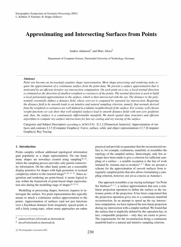
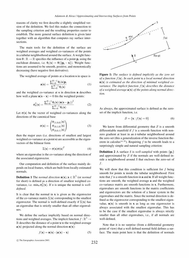
We define the surface implicitly based on normal direc-tions and weighted averages. The implicit function f : R

3 →R describes the distance of a point x to the weighted averagea(x) projected along the normal direction n(x):

f (x) = n(x) · (a(x)−x) (5)

x

n n(x-p)

a(x) f

S

(x)q

l

Figure 1: The surface is defined implicitly as the zero setof a function f (x). In each point x a local normal directionn(x) is estimated as the direction of minimal weighted co-variance. The implicit function f (x) describes the distanceof a weighted average a(x) of the points along normal direc-tion.

As always, the approximated surface is defined as the zero-set of the implicit function, i.e.

S = {x : f (x) = 0} (6)

We know from differential geometry that S is a smoothdifferentiable manifold if f is a smooth function with non-zero gradient at least in an ε-tubular neighborhood aroundthe zero-set (this a generalization of the inverse function the-orem in calculus14, 25). Requiring f to be smooth leads to asurprisingly simple and natural sampling criterion:

Definition 2 A surface S is well-sampled with points {pi}and approximated by S if the normals are well-defined in-side a neighborhood around S that encloses the zero-set off .

We will show that this condition is sufficient for f beingsmooth for points x inside the tubular neighborhood: Firstnote that f is a smooth function in a and n. If all weight func-tions are smooth, the weighted average a and the weightedco-variance matrix are smooth functions in x. Furthermore,eigenvalues are smooth functions in the matrix coefficientsand eigenvectors are the solution of a linear system in theeigenvalues and the matrix. Since the normal direction is de-fined as the eigenvector corresponding to the smallest eigen-value, n(x) is smooth in x as long as one eigenvector isalways associated with the smallest eigenvalue. This hasto be the case if the smallest eigenvalue is always strictlysmaller than all other eigenvalues, i.e., if all normals arewell-defined.

Note that it is no surprise (from a differential geometrypoint of view) that a well defined normal field defines a sur-face. The main point here is that the definition of normals



as directions of smallest weighted co-variance admits such adefinition.

The topology of the approximated surface S depends onthe particular choice of weight functions θi. It is clear thatcertain θi could lead to non-manifold approximations andthat even if S is manifold it’s not necessarily homeomorphicto S. On the other hand, weights could be so chosen thatS is manifold and, with further restrictions, resembles thetopology of S.

To give an intuition for this, we first consider an infinites-imal ball B around s. Inside the ball, weights are constantand so are a(x) and n(x). Thus, for this region f describes aplane and if this plane passes the ball the approximation ofS inside B is a disk. If, furthermore, the gradient of f insidesuch ball is non-zero, S is manifold. We show in the Ap-pendix that using Gaussians as weight functions is sufficientfor non-zero gradient at f (x) = 0.

For homeomorphic reconstruction the support of theweights should be so chosen that they separate differentsheets of the surface (note that sufficient sampling is a pre-requisite for differentiation of sheets). As Gaussians have in-finite support we have no practical means to construct theo-retically correct weights yet, however, in practice Gaussianswith appropriate radius perform quite nicely (as is demon-strated in Section 6).

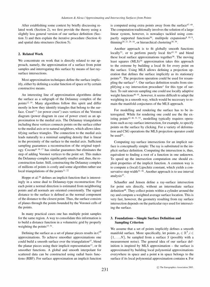
4. Ray-surface intersections

The surface definition given in the previous section impliesa technique to efficiently compute ray-surface intersections.The idea is to evaluate function f , as it provides a roughapproximation of the distance field to S for f (x) 6= 0. Forfixed n and a Equation 5 describes the planar fit

l(x) = n(s) · (a(s)−x) (7)

to S with respect to the location s (depicted by the dashedline in Figure 1). The smaller the distance f (s) is, the betterS is approximated in q, which is the projection of x onto lalong n. If f (s) = 0, q = s is a point on the surface S.

The approximation l is used to converge to S along a ray r,using an iterative scheme similar to the ray tracing approachfor MLS-surfaces1. Once an approximation is determined,the equation r = ro + s · td is inserted in l(x), and solvingl(r) = 0 provides td for the intersection of ray and planarsurface approximation. The series of intersections {ri} ap-proaches the surface S. In theory, once ri is close enoughto the surface, the series | f (ri)|, | f (ri+1)|, | f (ri+2)|, . . . isstrictly decreasing and an increase could be used to bail outoff the iteration and start over. In practice, however, we haveto accommodate imperfect weighting and use more tolerantiteration conditions: We require that the closest point q onthe approximated surface is close to the current position onthe ray ri that has been used to compute q as well as closeto the next intersection ri+1 of the ray and the plane l = 0

H

Surface

Ray

n

r i

Figure 2: In an intermediate approximation of the ray sur-face intersection ri a local coordinate system H is estab-lished using the direction of minimal weighted co-varianceas the normal n

through q. Specifically, a region of trust T around q has tocontain ri and ri+1. If not, the iteration is terminated andno ray surface intersection in the proximity of r0 could bereported.

How to obtain an initial point r0 is discussed later in Sec-tion 5. The region T depends on the weighting-function forn(x) and a(x), which affects the size of features in S. Howto make suitable choices for the weighting-function and T isalso addressed in Section 5.

The procedure sketched above is easily generalized bytaking the following point of view: In each point on r a localcoordinate system is created using the approximation of anormal direction. In this coordinate system a weighted leastsquare constant approximation to the surface is computed(the weighted average is a constant least squares approxima-tion). This local approximation is intersected with the rayand the procedure is repeated. In this setting it seems quitenatural to use higher order least squares approximations tothe surface in the local coordinate system in an attempt toincrease the approximation order of the scheme. In retro-spect, we have used constant polynomials for the analysisbecause this allows explicitly solving the linear system thatdetermines the polynomial.

The following three steps are iterated until the sequencer0,r1,r2, ... converges to the ray-surface intersection or theprocedure is terminated, focussing on the next region to beexamined:

1. Support plane: The normal of a support plane H in ri isdetermined by minimizing the weighted distances of thepoints p j to H. The weights are computed from the dis-tances of the p j to ri using a smooth, positive, monotone

decreasing function θ (e.g. a gaussian θ(d) = e−d2

h2 ). This



weighted least squares problem is solved by minimizing

N

∑j=1

(

〈n,p j − ri〉)2θ

(

‖p j − ri‖)

, (8)

The minimization of equation 8 can be rewritten in bilin-ear form

min‖n‖=1

nT Bn, (9)

where B = {bkl} is the matrix of weighted co-variances

blk =N

∑j=1

θ j(

p jk − rik)(

p jl − ril)

.

The minimization problem in equation 9 is solved bycomputing the eigenvector of B with the smallest eigen-value. The resulting H is approximately parallel to theSurface in the area around its nearest approach to ri.

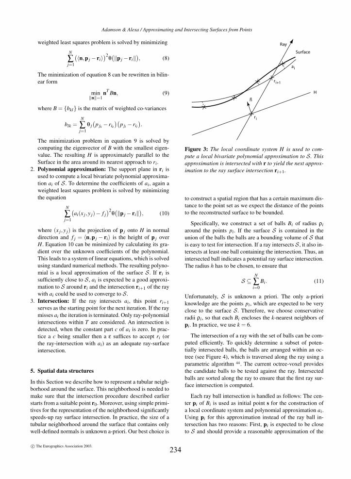
2. Polynomial approximation: The support plane in ri isused to compute a local bivariate polynomial approxima-tion ai of S. To determine the coefficients of ai, again aweighted least squares problem is solved by minimizingthe equation

N

∑j=1

(

ai(x j,y j)− f j)2θ

(

‖p j − ri‖)

, (10)

where (x j,y j) is the projection of p j onto H in normaldirection and f j = 〈n,p j − ri〉 is the height of p j overH. Equation 10 can be minimized by calculating its gra-dient over the unknown coefficients of the polynomial.This leads to a system of linear equations, which is solvedusing standard numerical methods. The resulting polyno-mial is a local approximation of the surface S. If ri issufficiently close to S, ai is expected be a good approxi-mation to S around ri and the intersection ri+1 of the raywith ai could be used to converge to S.

3. Intersection: If the ray intersects ai, this point ri+1serves as the starting point for the next iteration. If the raymisses ai the iteration is terminated. Only ray-polynomialintersections within T are considered. An intersection isdetected, when the constant part c of ai is zero. In prac-tice a c being smaller then a ε suffices to accept ri (orthe ray-intersection with ai) as an adequate ray-surfaceintersection.

5. Spatial data structures

In this Section we describe how to represent a tubular neigh-borhood around the surface. This neighborhood is needed tomake sure that the intersection procedure described earlierstarts from a suitable point r0. Moreover, using simple primi-tives for the representation of the neighborhood significantlyspeeds-up ray surface intersection. In practice, the size of atubular neighborhood around the surface that contains onlywell-defined normals is unknown a-priori. Our best choice is

H

Surface

Ray

n

a i

r i

ri+1

Figure 3: The local coordinate system H is used to com-pute a local bivariate polynomial approximation to S. Thisapproximation is intersected with r to yield the next approx-imation to the ray surface intersection ri+1.

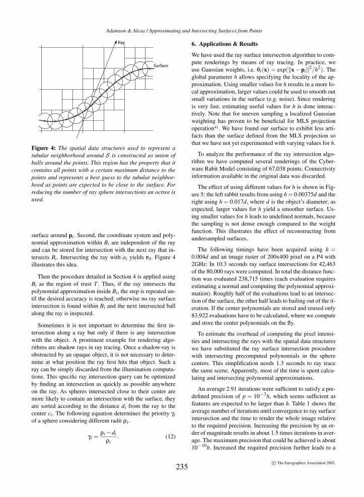
to construct a spatial region that has a certain maximum dis-tance to the point set as we expect the distance of the pointsto the reconstructed surface to be bounded.

Specifically, we construct a set of balls Bi of radius ρiaround the points pi. If the surface S is contained in theunion of the balls the balls are a bounding volume of S thatis easy to test for intersection. If a ray intersects S, it also in-tersects at least one ball containing the intersection. Thus, anintersected ball indicates a potential ray surface intersection.The radius h has to be chosen, to ensure that

S ⊆N

∑i=0

Bi. (11)

Unfortunately, S is unknown a priori. The only a-prioriknowledge are the points pi, which are expected to be veryclose to the surface S. Therefore, we choose conservativeradii ρi, so that each Bi encloses the k-nearest neighbors ofpi. In practice, we use k = 6.

The intersection of a ray with the set of balls can be com-puted efficiently. To quickly determine a subset of poten-tially intersected balls, the balls are arranged within an oc-tree (see Figure 4), which is traversed along the ray using aparametric algorithm 44. The current octree-voxel providesthe candidate balls to be tested against the ray. Intersectedballs are sorted along the ray to ensure that the first ray sur-face intersection is computed.

Each ray ball intersection is handled as follows: The cen-ter pi of Bi is used as initial point s for the construction ofa local coordinate system and polynomial approximation ai.Using pi for this approximation instead of the ray ball in-tersection has two reasons: First, pi is expected to be closeto S and should provide a reasonable approximation of the



Surface

Ray

Figure 4: The spatial data structures used to represent atubular neighborhood around S is constructed as union ofballs around the points. This region has the property that itcontains all points with a certain maximum distance to thepoints and represents a best guess to the tubular neighbor-hood as points are expected to be close to the surface. Forreducing the number of ray sphere intersections an octree isused.

surface around pi. Second, the coordinate system and poly-nomial approximation within Bi are independent of the rayand can be stored for intersection with the next ray that in-tersects Bi. Intersecting the ray with ai yields r0. Figure 4illustrates this idea.

Then the procedure detailed in Section 4 is applied usingBi as the region of trust T . Thus, if the ray intersects thepolynomial approximation inside Bi, the step is repeated un-til the desired accuracy is reached; otherwise no ray surfaceintersection is found within Bi and the next intersected ballalong the ray is inspected.

Sometimes it is not important to determine the first in-tersection along a ray but only if there is any intersectionwith the object. A prominent example for rendering algo-rithms are shadow rays in ray tracing. Once a shadow-ray isobstructed by an opaque object, it is not necessary to deter-mine at what position the ray first hits that object. Such aray can be simply discarded from the illumination computa-tions. This specific ray intersection query can be optimizedby finding an intersection as quickly as possible anywhereon the ray. As spheres intersected close to their center aremore likely to contain an intersection with the surface, theyare sorted according to the distance di from the ray to thecenter ci. The following equation determines the priority γiof a sphere considering different radii ρi.

γi =ρi −di

ρi. (12)

6. Applications & Results

We have used the ray surface intersection algorithm to com-pute renderings by means of ray tracing. In practice, weuse Gaussian weights, i.e. θi(x) = exp(‖x− pi‖

2/h2). Theglobal parameter h allows specifying the locality of the ap-proximation. Using smaller values for h results in a more lo-cal approximation, larger values could be used to smooth outsmall variations in the surface (e.g. noise). Since renderingis very fast, estimating useful values for h is done interac-tively. Note that for uneven sampling a localized Gaussianweighting has proven to be beneficial for MLS projectionoperation41. We have found our surface to exhibit less arti-facts than the surface defined from the MLS projection sothat we have not yet experimented with varying values for h.

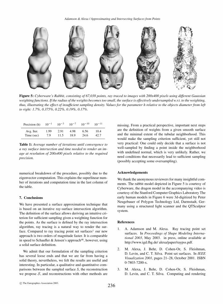
To analyze the performance of the ray intersection algo-rithm we have computed several renderings of the Cyber-ware Rabit Model consisting of 67,038 points. Connectivityinformation available in the original data was discarded.

The effect of using different values for h is shown in Fig-ure 5: the left rabbit results from using h = 0.00375d and theright using h = 0.017d, where d is the object’s diameter; asexpected, larger values for h yield a smoother surface. Us-ing smaller values for h leads to undefined normals, becausethe sampling is not dense enough compared to the weightfunction. This illustrates the effect of reconstructing fromundersampled surfaces.

The following timings have been acquired using h =0.004d and an image raster of 200x400 pixel on a P4 with2GHz: In 10.3 seconds ray surface intersections for 42,463of the 80,000 rays were computed. In total the distance func-tion was evaluated 238,715 times (each evaluation requiresestimating a normal and computing the polynomial approxi-mation). Roughly half of the evaluations lead to an intersec-tion of the surface, the other half leads to bailing out of the it-eration. If the center polynomials are stored and reused only83,922 evaluations have to be calculated, where we computeand store the center polynomials on the fly.

To estimate the overhead of computing the pixel intensi-ties and intersecting the rays with the spatial data structureswe have substituted the ray surface intersection procedurewith intersecting precomputed polynomials in the spherecenters. This simplification needs 1.3 seconds to ray tracethe same scene. Apparently, most of the time is spent calcu-lating and intersecting polynomial approximations.

An average 2.91 iterations were sufficient to satisfy a pre-defined precision of p = 10−3h, which seems sufficient asfeatures are expected to be larger than h. Table 1 shows theaverage number of iterations until convergence to ray surfaceintersection and the time to render the whole image relativeto the required precision. Increasing the precision by an or-der of magnitude results in about 1.5 times iterations in aver-age. The maximum precision that could be achieved is about10−10h. Increased the required precision further leads to a



Figure 5: Cyberware’s Rabbit, consisting of 67,038 points, ray traced to images with 200x400 pixels using different Gaussianweighting functions. If the radius of the weights becomes too small, the surface is effectively undersampled w.r.t. to the weighting,thus, illustrating the effect of insufficient sampling density. Values for the parameter h relative to the objects diameter from leftto right: 1.7%, 0.375%, 0.22%, 0.19%, 0.17%.

Precision (h) 10−1 10−3 10−7 10−10 10−11

Avg. Iter. 1.99 2.91 4.98 6.56 10.4Time (sec) 7.9 11.5 18.9 24.6 42.7

Table 1: Average number of iterations until convergence toa ray surface intersection and time needed to render an im-age at resolution of 200x400 pixels relative to the requiredprecision.

numerical breakdown of the procedure, possibly due to theeigenvector computation. This explains the superlinear num-ber of iterations and computation time in the last column ofthe table.

7. Conclusions

We have presented a surface approximation technique thatis based on an iterative ray-surface intersection algorithm.The definition of the surface allows deriving an intuitive cri-terion for sufficient sampling given a weighting function forthe points. As the surface is defined by the ray intersectionalgorithm, ray tracing is a natural way to render the sur-face. Compared to ray tracing point set surfaces1 our newapproach is two orders of magnitude faster. It is comparablein speed to Schaufler & Jensen’s approach48, however, usinga solid surface definition.

We admit that our formulation of the sampling criterionhas several loose ends and that we are far from having asolid theory, nevertheless, we felt the results are useful andinteresting. In particular, a qualitative and quantitative com-parisons between the sampled surface S, the reconstructionwe propose S, and reconstructions with other methods are

missing. From a practical perspective, important next stepsare the definition of weights from a given smooth surfaceand the minimal extent of the tubular neighborhood. Thiswould make the sampling criterion sufficient, yet still notvery practical: One could only decide that a surface is notwell-sampled by finding a point inside the neighborhoodwith undefined normal, which is very unlikely. Rather, weneed conditions that necessarily lead to sufficient sampling(possibly accepting some oversampling).

Acknowledgements

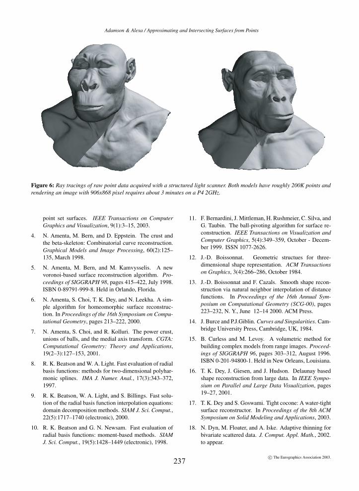
We thank the anonymous reviewers for many insightful com-ments. The rabbit model depicted in Figure 5 is courtesy ofCyberware, the dragon model in the accompanying video iscourtesy of the Stanford Computer Graphics Laboratory Theearly human models in Figure 6 were 3d-digitized by PeterNeugebauer of Polygon Technology Ltd, Darmstadt, Ger-many using a structured light scanner and the QTSculptorsystem.

References

1. A. Adamson and M. Alexa. Ray tracing point setsurfaces. In Proceedings of Shape Modeling Interna-tional 2003, May 2003. in press, online available athttp://www.igd.fhg.de/ alexa/paper/raypss.pdf.

2. M. Alexa, J. Behr, D. Cohen-Or, S. Fleishman,D. Levin, and C. T. Silva. Point set surfaces. In IEEEVisualization 2001, pages 21–28, October 2001. ISBN0-7803-7200-x.

3. M. Alexa, J. Behr, D. Cohen-Or, S. Fleishman,D. Levin, and C. T. Silva. Computing and rendering



Figure 6: Ray tracings of raw point data acquired with a structured light scanner. Both models have roughly 200K points andrendering an image with 906x868 pixel requires about 3 minutes on a P4 2GHz.

point set surfaces. IEEE Transactions on ComputerGraphics and Visualization, 9(1):3–15, 2003.

4. N. Amenta, M. Bern, and D. Eppstein. The crust andthe beta-skeleton: Combinatorial curve reconstruction.Graphical Models and Image Processing, 60(2):125–135, March 1998.

5. N. Amenta, M. Bern, and M. Kamvysselis. A newvoronoi-based surface reconstruction algorithm. Pro-ceedings of SIGGRAPH 98, pages 415–422, July 1998.ISBN 0-89791-999-8. Held in Orlando, Florida.

6. N. Amenta, S. Choi, T. K. Dey, and N. Leekha. A sim-ple algorithm for homeomorphic surface reconstruc-tion. In Proceedings of the 16th Symposium on Compu-tational Geometry, pages 213–222, 2000.

7. N. Amenta, S. Choi, and R. Kolluri. The power crust,unions of balls, and the medial axis transform. CGTA:Computational Geometry: Theory and Applications,19(2–3):127–153, 2001.

8. R. K. Beatson and W. A. Light. Fast evaluation of radialbasis functions: methods for two-dimensional polyhar-monic splines. IMA J. Numer. Anal., 17(3):343–372,1997.

9. R. K. Beatson, W. A. Light, and S. Billings. Fast solu-tion of the radial basis function interpolation equations:domain decomposition methods. SIAM J. Sci. Comput.,22(5):1717–1740 (electronic), 2000.

10. R. K. Beatson and G. N. Newsam. Fast evaluation ofradial basis functions: moment-based methods. SIAMJ. Sci. Comput., 19(5):1428–1449 (electronic), 1998.

11. F. Bernardini, J. Mittleman, H. Rushmeier, C. Silva, andG. Taubin. The ball-pivoting algorithm for surface re-construction. IEEE Transactions on Visualization andComputer Graphics, 5(4):349–359, October - Decem-ber 1999. ISSN 1077-2626.

12. J.-D. Boissonnat. Geometric structues for three-dimensional shape representation. ACM Transactionson Graphics, 3(4):266–286, October 1984.

13. J.-D. Boissonnat and F. Cazals. Smooth shape recon-struction via natural neighbor interpolation of distancefunctions. In Proceedings of the 16th Annual Sym-posium on Computational Geometry (SCG-00), pages223–232, N. Y., June 12–14 2000. ACM Press.

14. J. Burce and P.J.Giblin. Curves and Singularities. Cam-bridge University Press, Cambridge, UK, 1984.

15. B. Curless and M. Levoy. A volumetric method forbuilding complex models from range images. Proceed-ings of SIGGRAPH 96, pages 303–312, August 1996.ISBN 0-201-94800-1. Held in New Orleans, Louisiana.

16. T. K. Dey, J. Giesen, and J. Hudson. Delaunay basedshape reconstruction from large data. In IEEE Sympo-sium on Parallel and Large Data Visualization, pages19–27, 2001.

17. T. K. Dey and S. Goswami. Tight cocone: A water-tightsurface reconstructor. In Proceedings of the 8th ACMSymposium on Solid Modeling and Applications, 2003.

18. N. Dyn, M. Floater, and A. Iske. Adaptive thinning forbivariate scattered data. J. Comput. Appl. Math., 2002.to appear.



19. H. Edelsbrunner and E. P. Mücke. Three-dimensionalalpha shapes. ACM Transactions on Graphics,13(1):43–72, January 1994. ISSN 0730-0301.

20. M. S. Floater and A. Iske. Multistep scattered datainterpolation using compactly supported radial basisfunctions. J. Comput. Appl. Math., 73(1-2):65–78,1996.

21. M. S. Floater and A. Iske. Thinning algorithms for scat-tered data interpolation. BIT, 38(4):705–720, 1998.

22. M. Gopi, S. Krishnan, and C. T. Silva. Surface recon-struction based on lower dimensional localized delau-nay triangulation. Computer Graphics Forum, 19(3),August 2000.

23. A. Goshtasby and W. D. O’Neill. Surface fitting to scat-tered data by a sum of gaussians. Computer Aided Ge-ometric Design, 10(2):143–156, April 1993.

24. M. Gross. Are points the better graphics primitives?Computer Graphics Forum, 20(3), 2001. ISSN 1067-7055.

25. V. Guillemin and A. Pollack. Differential Topology.Prentice-Hall Inc., Englewood Cliffs, 1974.

26. J. C. Hart. Sphere tracing: a geometric method for theantialiased ray tracing of implicit surfaces. The VisualComputer, 12(9):527–545, 1996. ISSN 0178-2789.

27. H. Hoppe, T. DeRose, T. Duchamp, M. Halstead,H. Jin, J. McDonald, J. Schweitzer, and W. Stuetzle.Piecewise smooth surface reconstruction. Proceedingsof SIGGRAPH 94, pages 295–302, July 1994. ISBN0-89791-667-0. Held in Orlando, Florida.

28. H. Hoppe, T. DeRose, T. Duchamp, J. McDonald,and W. Stuetzle. Surface reconstruction from unor-ganized points. Computer Graphics (Proceedings ofSIGGRAPH 92), 26(2):71–78, July 1992. ISBN 0-201-51585-7. Held in Chicago, Illinois.

29. A. Iske. Hierarchical scattered data filtering for multi-level interpolation schemes. In Mathematical methodsfor curves and surfaces (Oslo, 2000), pages 211–221.Vanderbilt Univ. Press, Nashville, TN, 2001.

30. A. Iske and J. Levesley. Multilevel scattered data ap-proximation by adaptive domain decomposition. Tech-nical report, 2002. Preprint.

31. A. Kalaiah and A. Varshney. Differential point render-ing. In Rendering Techniques 2001: 12th EurographicsWorkshop on Rendering, pages 139–150. Eurographics,June 2001. ISBN 3-211-83709-4.

32. D. Kalra and A. H. Barr. Guaranteed ray intersec-tions with implicit surfaces. Computer Graphics (Pro-ceedings of SIGGRAPH 89), 23(3):297–306, July 1989.Held in Boston, Massachusetts.

33. Z. Lei, M. M. Blane, and D. B. Cooper. 3L fitting ofhigher degree implicit polynomials. In Proceedings ofThird IEEE Workshop on Applications of Computer Vi-sion, Sarasota, Florida, USA, Dec. 1996.

34. D. Levin. The approximation power of moving least-squares. Mathematics of Computation, 67(224), 1998.

35. D. Levin. Mesh-independent surface interpolation,2003.

36. M. Levoy, K. Pulli, B. Curless, S. Rusinkiewicz,D. Koller, L. Pereira, M. Ginzton, S. Anderson,J. Davis, J. Ginsberg, J. Shade, and D. Fulk. The dig-ital michelangelo project: 3d scanning of large statues.Proceedings of SIGGRAPH 2000, pages 131–144, July2000. ISBN 1-58113-208-5.

37. D. P. Mitchell. Robust ray intersection with intervalarithmetic. Graphics Interface ’90, pages 68–74, May1990.

38. Y. Ohtake, A. Belyaev, M. Alexa, G. Turk, and H.-P.Seidel. Multi-level partition of unity implicits. ACMTransactions on Computer Graphics (SIGGRAPH 2003Proceedings), 22(3), 2003.

39. Y. Ohtake, A. Belyaev, and H.-P. Seidel. A multi-scale approach to 3d scattered data interplation withcompactly supported basis functions. In Proceedingsof Shape Modeling International 2003, May 2003. inpress.

40. M. Pauly, M. Gross, and L. P. Kobbelt. Efficient sim-plification of point-sampled surfaces. In R. Moorhead,M. Gross, and K. I. Joy, editors, Proceedings of the 13thIEEE Visualization 2002 Conference (VIS-02), pages163–170, Piscataway, NJ, Oct. 27– Nov. 1 2002. IEEEComputer Society.

41. M. Pauly, R. Kaiser, L. Kobbelt, and M. Gross. Shapemodeling with point-sampled geometry. ACM Trans-actions on Graphics (SIGGRAPH 2003 issue), 22(3),2003. to appear.

42. H. Pfister, M. Zwicker, J. van Baar, and M. Gross. Sur-fels: Surface elements as rendering primitives. Pro-ceedings of SIGGRAPH 2000, pages 335–342, July2000. ISBN 1-58113-208-5.

43. V. Pratt. Direct least-squares fitting of algebraic sur-faces. Computer Graphics (Proceedings of SIGGRAPH87), 21(4):145–152, July 1987. Held in Anaheim, Cal-ifornia.

44. J. Revelles, C. Urena, and M. Lastra. An efficient para-metric algorithm for octree traversal. In WSCG 2000Conference Proceedings, 2000.

45. S. Rusinkiewicz, O. Hall-Holt, and M. Levoy. Real-time 3d model acquisition. ACM Transactions onGraphics, 21(3):438–446, July 2002. ISSN 0730-0301(Proceedings of ACM SIGGRAPH 2002).



46. S. Rusinkiewicz and M. Levoy. Qsplat: A multiresolu-tion point rendering system for large meshes. Proceed-ings of SIGGRAPH 2000, pages 343–352, July 2000.ISBN 1-58113-208-5.

47. V. V. Savchenko, A. A. Pasko, O. G. Okunev, and T. L.Kunii. Function representation of solids reconstructedfrom scattered surface points and contours. ComputerGraphics Forum, 14(4):181–188, October 1994.

48. G. Schaufler and H. W. Jensen. Ray tracing point sam-pled geometry. Rendering Techniques 2000: 11th Euro-graphics Workshop on Rendering, pages 319–328, June2000. ISBN 3-211-83535-0.

49. G. Turk and J. F. O’Brien. Modelling with implicit sur-faces that interpolate. ACM Transactions on Graphics,21(4):855–873, Oct. 2002.

50. H. Wendland. Piecewise polynomial, positive definiteand compactly supported radial functions of minimaldegree. Adv. Comput. Math., 4(4):389–396, 1995.

51. M. Wheeler, Y. Sato, and K. Ikeuchi. Consensus sur-faces for modeling 3d objects from multiple range im-ages. In IEEE International Conference on ComputerVision 1998, pages 917–924, 1998.

52. M. Zwicker, M. Pauly, O. Knoll, and M. Gross.Pointshop 3d: An interactive system for point-basedsurface editing. ACM Transactions on Graphics,21(3):322–329, July 2002. ISSN 0730-0301 (Proceed-ings of ACM SIGGRAPH 2002).

53. M. Zwicker, H. Pfister, J. van Baar, and M. Gross.Ewa splatting. IEEE Transactions on Visualization andComputer Graphics, 8(3):223–238, July - September2002. ISSN 1077-2626.

Appendix A: A sufficient condition for manifoldreconstruction

To guarantee that f (x) = 0 is manifold (assuming that thesurface is well-sampled and, thus, f is smooth) we have toshow that ∇ f (x) 6= 0 for f (x) = 0. We differentiate alongnormal direction in x to reduce the problem to one dimen-sion. Note that this is possible because the surface is well-sampled, which implies that normals are well-defined. Wecan re-write f in a coordinate system with the origin on thesurface along the dimension in normal direction as

f (ξ) = n(ξ)(a(ξ)−ξ) =∑θi(ξ)(ξ−φi)

2

∑θi(ξ)

(

∑θi(ξ)φi

∑θi(ξ)−ξ

)

(13)where φi denotes the distance of pi along normal direction.Since we have defined differentiation w.r.t. ξ in direction ofthe normal n, f (ξ) = 0 implies a(ξ) = 0 so that we have toshow only a′(ξ) to be non-zero:

a′(ξ) =∑θ′i(ξ)φi ∑θi(ξ)−∑θi(ξ)φi ∑θ′i(ξ)

(∑θi(ξ))2 −1 6= 0 (14)

A particular simple way to satisfy this inequality is to usestrictly positive weight functions of the form θ′ = cθ (i.e.exponential functions) because then the nominator is equalzero and the denominator is strictly positive. However, alsoGaussian weight functions

θi(h) = e|ξ−φi|/h2(15)

satisfy Eq. 14 for almost all h: The main observation is that

∑θ′i(h)φi ∑θi(h)−∑θi(h)φi ∑θ′i(h)−∑θi(h)∑θi(h)(16)

is a smooth function in h, whose gradient cannot vanisheverywhere because the Gaussians have strictly positivederivatives for positive values of h. Thus, Eq. 16 is smoothlyvarying with h and has only finitely many zeroes. All h thatequate to non-zero values are sufficient for a local manifoldreconstruction. Note that this is not sufficient for the exis-tence of a global h that guarantees manifoldness everywhereon the surface, on the other hand, it is very unlikely in prac-tice that the set of forbidden h-values all over the zero-setof f is dense in R. A better characterization of admissiblevalues for h is, nevertheless, desirable.


Approximating and Intersecting Surfaces from PointsApproximating and Intersecting Surfaces from...

Documents

Transcript of Approximating and Intersecting Surfaces from PointsApproximating and Intersecting Surfaces from...