sS|MP^FIEf:MEffODS;;FOR INTEilPREl|lN(5TjiE? PEE|T|' Ol itANSFER-EUNC'TION ZERpS;i«6fc OME fikNSlMTIRESPONSE'OF^AIRCRABT^

-,! "»• ! * -*' ?•• * < *

? v

?

'r! - > ?;

' |l.i^r / ' -%* ^Reiser <i>nkevli \ '' - , % > : . < ,

' ' ' I , ' * C--KJ ' f x< ' . / ' / ', '

if

f ^fl

https://ntrs.nasa.gov/search.jsp?R=19720019374 2018-08-23T03:01:21+00:00Z

1. RePorJrtlpjA FT™* Y 9'Sft'S 2' Government Accession No. 3. Recipient's Catalog No.

4. Title and Subtitle 5. Report Date

SIMPLIFIED METHODS FOR INTERPRETING THE EFFECT OF TRANSFER- July 1972FUNCTION ZEROS ON THE TRANSIENT RESPONSE OF AIRCRAFT 6. Performing Organization Code

7. Author(s) 8. Performing Organization Report No.

Reiner Onken A-Ul80

10. Work Unit No.9. Performing Organization Name and Address 135-19-02-01*

NASA Ames Research Center 11 Contract or GrantMoffett Field, Calif., 9^035

No.

13. Type of Report and Period Covered12. Sponsoring Agency Name and Address Technical Memorandum

National Aeronautics and Space Administration 14. Sponsoring AgencyWashington, D. C. 205^6

Code

15. Supplementary Notes

16. Abstract

Two simple methods are outlined for evaluating the effect of transfer- function zeros on thesystem time response. The pole effects can also be evaluated. These methods are useful forsimplified analysis or creating design criteria in terms of desirable regions of pole-zero locations

The type of transfer function studied is limited to those of linear systems. Correspondingto ordinary longitudinal or lateral aircraft transfer functions, the denominator polynomial is offourth order and tile numerator of third order at nest.

With the longitudinal motion of the aircraft as an example, the methods are used in theevaluation of optisial regulator control with respect to a particular performance index structure.

17. Key Words (Suggested by Author(s)) 18. Distribution Statement

ControlDynamic characteristics ._J . . . . Unclassified - UnlimitedRoots of equations

19. Security Qassif. (of this report) 20. Security Classif. (of this page) . .. 21. No. of PagesUnclassified , -t Unclassified- ' ' • ' 44

* t ' '

22. Price*

$3.00

' For sale by the National Technical Information Service, Springfield, Virginia 22151

TABLE OF CONTENTS

Page

SYMBOLS v

SUMMARY 1

INTRODUCTION 1

RESIDUE INTERPRETATION METHOD 2

Transfer Function and Transient Response Residues 2Phase Loci of the Residues UMagnitude Loci of the Residues . . . 7Interpretation of Pole Modifications 11

APPROXIMATE MODAL EXPANSION METHOD 12

Modal-Type Transfer Function Expansion (Two Zeros) 12Zero Loci Due to the B Values 13Three Zeros IT

EVALUATION OF OPTIMAL LONGITUDINAL CONTROL TIME RESPONSE WITH USE OFPOLE-ZERO INTERPRETATION METHODS 19

Problem Formulation 19Performance Criterion 20Discussion of Resulting Optimal Transfer Functions 21

CONCLUDING REMARKS 32

APPENDIX A - EQUATION FOR THE MAGNITUDE LOCI OF C±z (TWO ZEROS) .... 33

APPENDIX B - ENCIRCLING OF ZERO REGIONS FOR GIVEN VALUES OF |ciz| ... 3^

Region I 35Region II 35Region III 37

REFERENCES 38

iii

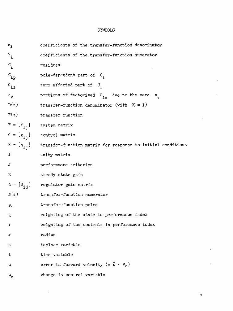
SYMBOLS

a^ coefficients of the transfer-function denominator

b. coefficients of the transfer-function numerator

C. residues

C. pole-dependent part of C.

C. zero effected part of C.

c portions of factorized C. due to the zero z

D(s) transfer-function denominator (with K = l)

F(S) transfer function

F = [f..] system matrix^-J

G = [g.j] control matrix-j

H = [h..] transfer-function matrix for response to initial conditions

I unity matrix

J performance criterion

K steady-state gain

L = [a. .] regulator gain matrix•*• J

N(S) transfer-function numerator

p. transfer-function poles

q weighting of the state in performance index

r weighting of the controls in performance index

r radius

s Laplace variable

t time variable

u error in forward velocity (= u • Vc)

u change in control variable

V command forward speed (equilibrium speed)

w error in vertical velocity

x state variable

z. transfer-function zeros

3 TTT transfer-function expansion coefficients_L ^ _L J_ J..L. J-

e damping angle

6 change in elevator control deflection

6_ change in direct lift control deflectionr

6 change in thrust control deflection

^l,¥>2 angles, defined in figures 2 and h

V phase-angle contribution of the C. denominator1\ Z 1Z

4>. phase angle of C.1 1Z

Y error in glide-path angle

6 error in longitudinal attitude (pitch angle)

o. real part of p. (damping)

a real part of poles Pi,2 (damping of eigenmode l)

a real part of pair of zeros

a coordinate of the centers of zero loci circles on the real axiszm

to eigenmode frequency

co y natural frequency of eigenmode I

oj natural frequency of pair of zerosoz

to "eigenfrequency" of conjugate complex pair of zerosZ

<jj "eigenfrequency" of pair of real zerosZ

vi

SIMPLIFIED METHODS FOR INTERPRETING THE EFFECT

OF TRANSFER-FUNCTION ZEROS ON THE

TRANSIENT RESPONSE OF AIRCRAFT

Reiner Onken*

Ames Research Center

SUMMARY

Two simple methods are outlined for evaluating the effect of transfer-function zeros on the system time response. The pole effects can also beevaluated. These methods are useful for simplified analysis or creatingdesign criteria in terms of desirable regions of pole-zero locations.

The type of transfer function studied is limited to those of linear sys-tems. Corresponding to ordinary longitudinal or lateral aircraft transferfunctions, the denominator polynomial is of fourth order and the numerator ofthird order at most.

With the longitudinal motion of the aircraft- as an example, the methodsare used in the evaluation of optimal regulator control with respect to aparticular performance index structure.

INTRODUCTION

The dynamic behavior of a flight vehicle usually can be described by asystem of linearized differential equations with constant coefficients or bythe corresponding set of transfer functions. The use of feedback control inmultivariable systems makes it possible to modify not only the denominator ofthe transfer functions, but also the numerator. This property is desirablefor it leads to the additional possibility of improving the vehicle's dynamicbehavior. As an extreme case, nonminimum phase effects (numerator roots withpositive real component), which occur rather often in aircraft transfer func-tions, could be ruled out or at least be moderated by appropriate feedbackcontrol.

Therefore, some work was directed toward the development of methods forthe investigation of the numerator roots based on illustrative frequencydomain techniques (refs. 1-U). These techniques provide an estimate ofchanges in the numerator and denominator roots of the transfer functions as aconsequence of feedback loop gains. To establish design criteria in terms ofappropriate root locations, the effect of the zero locations on the dynamicbehavior, that is, time response, should be known. The time response appears*National Research Council Associate.

to be most suitable for evaluations of system behavior, since the necessity ofan analytical formulation of the performance index can be avoided. Systemtime response may be obtained by resolving the transfer functions into partialfraction series and taking the inverse term by term (residue calculation).This procedure is well known, but it does not offer a means of showing trans-parently what changes in the time response can be expected from certain pole-zero modifications. Especially for multivariable systems, a more effectiveprocedure is required. Various pole-zero configurations have to be evaluatedto determine the effect of modifications on the corresponding time histories.

This report discusses simple methods that show the effect of zeros andpoles on the transient response so that root locations can be assigned forcertain desirable transient response behavior. Two basic methods will bedescribed: The first is based on the assignment of phase and magnitude of theresidues to the root locations; the second, which is easily applicable to air-craft control systems, is based on a specific expansion of the transfer func-tions, where each expansion term itself has a known transient response.

The application of both methods is restricted to a controlled elementtransfer function with a fourth-order denominator and at most third-order-numerator. This typifies either the longitudinal or lateral directionalequations of motion of an aircraft.

Implementation of the methods is discussed for the evaluation of an air-craft optimal control system. The optimal longitudinal motion regulator withrespect to a particular quadratic performance index is evaluated for differ-ent relative weighting between the states and the controls.

RESIDUE INTERPRETATION METHOD

Transfer Function and Transient Response Residues

The transfer functions investigated here are of the fourth-order denom-inator and at most third-order numerator type. This is the structure of themain open-loop aircraft longitudinal motion transfer functions as well as thecorresponding closed-loop transfer functions with constant feedback gains. Ifuc is generally taken as the input and x as the output, the transferfunction becomes

(1)

Disgarding the case of multiple roots, in the frequency domain the response toa step input can be written as a partial fraction expansion:

/\ (-pl)(~P2) ("Ps) (-Pit) (s-Zi )(s-Z2) (s-Zs)* \ S ) —• / \ ~ ix / \ /" ~ \ /~ \ / " " "V" r \ i \ i \

C.

~ withi=o

The inverse is1+

(t) = I C. e"1" (3)X

i=o

The partial fraction expansion coefficients C^, weighting the different modesinvolved, are

C± = lim [(s - pi)x(s)] (10

Thus3

-Q _ £ V5! (C)

i- S c(Pi-Pu)/(-Pu)]u=l

Normalizing the transient response vith respect to the steady state (K = l)gives CQ = 1. The remaining residues "become

:i, • ci, (6>where

The entire residue expression has been separated into two main factors C^pand Ciz, similar to each other, where one part (Cip) consists only of poleterms, while the other part (Ciz) contains all zero-affected terms. Thus,covers the whole effect of the zeros on the residue.

The zero-affected portion C z consists of products of fractions whosefactors are complex numbers in terms of the poles and zeros. They could bedrawn in the root plane as vectors from the different zeros to the pole p^and the origin. For two zeros, four vectors would have to be investigated foreach residue. This is not convenient, and a different representation of thezero effect on the residues is desirable. Furthermore, the representationshould illuminate zero regions of similar effect. Such a representation isdeveloped in the following sections.

The pole-dependent portion C^p has a reciprocal structure to that ofC-[z. Thus, the influence of the poles on the residues can be considered in away similar to that of the zeros.

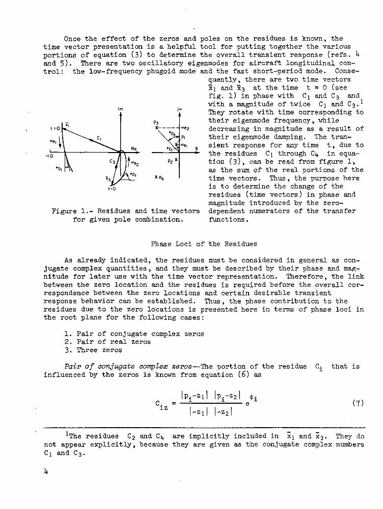
Once the effect of the zeros and poles on the residues is known, thetime vector presentation is a helpful tool for putting together the. variousportions of equation (3) to determine the overall transient response (refs. Uand 5). There are two oscillatory eigenmodes for aircraft longitudinal con-trol: the low-frequency phugoid mode and the fast short-period mode. Conse-

quently, there are two time vectorsxj and X3 at the time t = 0 (seefig. l) in phase with Ci and C$ andwith a magnitude of twice Cj and Cs- 1

They rotate with time corresponding totheir eigenmode frequency, while

2 decreasing in magnitude as a result oftheir eigenmode damping. The tran-

i g sient response for any time t, due to—*• the residues C\ through C^ in equa-

PZ x tion (3), can be read from figure 1,as the sum of the real portions of the

Xp4 time vectors. Thus, the purpose heret=0 is to determine the change of the

residues (time vectors) in phase andmagnitude introduced by the zero-

Figure 1.- Residues and time vectors dependent numerators of the transferfor given pole combination. functions.

t=0

-1.0

Phase Loci of the Residues

As already indicated, the residues must be considered in general as con-jugate complex quantities, and they must be described by their phase and mag-nitude for later use with the time vector representation. Therefore, the linkbetween the zero location and the residues is required before the overall cor-respondence between the zero locations and certain desirable transientresponse behavior can be established. Thus, the phase contribution to theresidues due to the zero locations is presented here in terms of phase loci inthe root plane for the following cases:

1. Pair of conjugate complex zeros2. Pair of real zeros3. Three zeros

Pair of conjugate complex zeros—The portion of the residueinfluenced by the zeros is known from equation (6) as

Ci that is

C. =iz\~Z2\

(7)

1The residues G£ and C^ are implicitly included in x^ and X3. They donot appear explicitly, because they are given as the conjugate complex numbersCi and Cq.

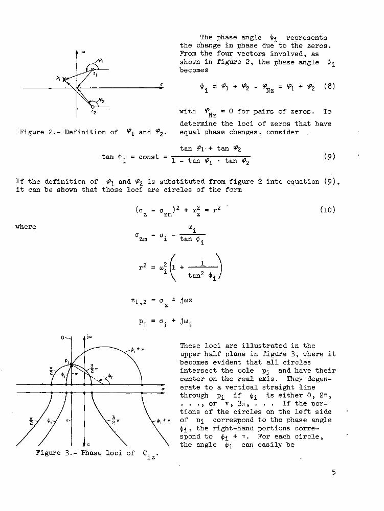
Figure 2.- Definition of f\ and ^2

tan *. = const

The phase angle <f>i representsthe change in phase due to the zeros.From the four vectors involved, asshown in figure 2, the phase angle <f>becomes

with V- = 0 for pairs of zeros. To

determine the loci of zeros that haveequal phase changes, consider

tan + tan_ tan

tan (9)

If the definition of #i and Y^ i-s substituted from figure 2 into equation (9),it can be shown that those loci are circles of the form

where

a - a )2 + u2 = r2z zm z (10)

to.j = a. - Tzm i tan q

tan

zl,2 =

jo,

p. = a. + jco.•^i i d i

Figure 3.- Phase loci

These loci are illustrated in theupper half plane in figure 3, where itbecomes evident that all circlesintersect the pole p^ and have theircenter on the real axis. They degen-erate to a vertical straight linethrough p^ if <f> is either 0, 27r,

or TT , 3ir, If the por-tions of the circles on the left sideof pi correspond to the phase angle<j>i, the right-hand portions corre-spond to <f»i + IT. For each circle,the angle ^i can easily be

determined as the angle between the real axis and the line connecting thecenter of the circle with p^.

Thus, each pair of conjugate complex zeros lying on one of the circlescauses the same phase shift <^_ on the residue C^ as any other pair "ofzeros on the same circle. The intersection points of the circles with thereal axis correspond to double zeros. This yields the link between the caseof conjugate complex zeros and that one of a pair of real zeros.

Pair of real zeros—The phase angle fa for the case of real zeros isalso given by equation (8) (see fig. U). The loci of pairs of real zeros sat-isfying the condition of equal phase changes are

(a _ a )2 _ -2 = r2 (11). z zm z

where

wia = a. -zm i tan $.

zl 2 = 0 * £01 **• zZ Z

i = a. + jco.

Drawing it in a oz,toz plane (thelower half plane in fig. 3), weobtain a set of rectangular hyperbolaswith their asymptotes inclined by ^5°to the real axis. For corresponding

—£ values of <j>^, the hyperbolas inter-sect the real axis at the same pointsas the circles for the case of conju-

Figure U.- Definition of "^ and 2 ga^6 complex pairs of zeros. Thus,for pair of real zeros. considering both the base of conjugate

complex zeros and that of a pair ofreal zeros, a certain range in the

residue phase angle will correspond to an area in the root plane, bounded bythe appropriate loci curves.

Three zeros—If the number of zeros is extended from two to three, theequation for the residue portion affected by the zeros Ciz is slightlychanged to

C.- = eiz

3

nV=l

-(12)

Figure 5-- Phase shiftto third zero 23.

due

Considering the phase loci, there isthe same family of curves in the rootplane as already derived, with anadditional phase shift A<J>^ due tothe third zero; that is,

(two zeros)(13)

where A^ can be easily derived forthe third zero moving along the realaxis, as shown in figure 5• There isa discontinuity in A^ of IT, whenZ3 passes the imaginary axis.

Magnitude Loci of the Residues

As outlined previously, a mapping of the magnitude, as well as the phase,of GI in the root plane by means of locus curves is required.. Following thesame line of reasoning as for the.phase effect of the zeros on C±z> oneobtains locus curves of higher order, which are too complicated for simplegeometrical interpretation (see appendix A). Therefore, the expression for|Ciz| will be split so that it can be discussed partially by simple geometri-cal means. Again, the cases of conjugate complex pairs of zeros, two realzeros, and three zeros are discussed.

Pair of conjugate complex zeros—Following equation (7), the magnitude ofis split into

I j_zl 1 2

where- zl - Z2

c2 =

Therefore, the two portions c\ and c2 are discussed separately and then their,|Ciproduct |Ciz. The loci curves in the root plane for both

are circles (fig. 6) given, respectively, byand again

and

(oz - a

(a - az

)2

)2

\2 =zmj

)O 9^ = r^zm2' Z2

(15)

(16)

where

Figure 6.- Magnitude loci of C]..

1 - c2 '

a.

1 --c.

0).

1 - c2 '0)

1 - c.

2 = (a2 + u,2). ' W . / •

1 " (1 - c2)2.2 =22

= (

(1 - c2)2

Both families of circles are very similar: the circles for 02 represent thesymmetrical image about the real axis of those with the same value for GI-Thus, only circles for GI are shown in figure 6; the straight line represent-ing C2 = 1 is added to show the symmetry.

The geometrical structure of the circles becomes obvious by consideringthe following properties (stated for the case of GI only):

1. The center points of the circles given by azm and tozm lie on thestraight line passing through p^ and the origin.

2. The radius of the locus circles for c^ = a and GJ = I/a is thesame. The corresponding center points lie symmetrical to the pointmidway between p^ and the origin. The midpoint is on the locuscircle for cj =1, which has degenerated to a straight line andintersects the real axis at

(IT)

The line for GI = 1 is thus the perpendicular bisector of the linebetween p^ and the origin.

3. The circles degenerate to a point at p^ or at the origin forvalues of GI going to either zero or infinity, respectively.

^. The radii of the circles are given by the product between thedistance of the center from the origin and the value of thecorresponding magnitude.

Considering the intersections of the GI and 02 circles, each suchintersection represents a value of \C±Z\ , given by the product of.GI and 02 at that point. Vice versa, for a given point in the rootplane, cj and 02 can be determined and then \C±Z\ itself.

Although the higher order loci curves of the magnitude of C z are givenby the intersections of two families of circles, it still is rather tedious toderive those curves for each required case without great computational effort.

A simpler interpretation can be obtained by encircling an area in theroot plane for zeros that correspond to the required ranges of |cn-,|. Thatmeans the exact locus curve for the required value ofapproximated by a surrounding region.

I *— . I J_ £j I

Ciz| will be

|ci2'|=i

©

Figure 7.- Examples of approximatezero locations for certainvalues of \C±z\•

Figure 7 shows the upper half ofthe root plane (the lower half wouldshow symmetrically the same), wherefor each of the three regions (I, II,III) separated by the locus curvesfor GI = 1 and C2 = 1, an example ofencircling is shown. Those examplesare based on the following statements.(More details are given in appendixB.)

Region I: (a) If \C±Z\ is distinc-tively greater than 1, the circle ofC2 = l^izl surrounds the area withinwhich all conjugate complex zeroscorresponding to that |C Z| mustlie (example, |Ciz| > 2.0). (b) If|Ciz| is distinctively smaller than1, the circle of cj = |Ciz|

surrounds the area within which all conjugate complex zeros corresponding tothat |Cj.z| must lie (example, |Ciz| < O.U).

Region II: All conjugate complex zeros corresponding to a certain valueof |C-:_| > 1 must lie within the union of the circles for c, = |c,-z| andQ ' i X «j I i . 1 ' J- ** 'C2 = l^izl ^u* outside the intersection of those circles (example,|Ciz| * 10).

Region III: All conjugate complex zeros corresponding to a certain valueof \£±z\ where

2 1 t 9 1 1must lie within the union of the circles for c1 = |C Z| and c2 = l^izloutside the intersection of those circles (example, |Ciz| • 0.3).

As the straight-line loci for GI = 1 and C2 = 1 separating the differentregions change with pj_, the circles encircling the zero regions are cut dif-ferently by those lines. However, the radii of the circles are proportionalto |p | and do not change if p^ remains constant in magnitude.

For the locus of |Cj_z| = 1, some other simplifying specifications can bemade. In the relations given in appendix A, it becomes, evident that the locusfor |Cj[z| = 1 intersects the real axis at the same point that the loci forGI = 1 and C2 = 1 intersect. The locus goes to infinity in its imaginarycoordinate for

a2 - co2

a, = \n X (18)z 2a.i

and at a = a. , u> is defined byz i' z J

2 , 9 -L | I /i /^ \u/ + at = -r p. (19)z i d ' i

Notice that equation (19) can hold only if the locus intersects the real axisat the left of the pole p^. Otherwise, the relation for (i)z at az = (l/2)amay be used, where

"z + ¥ ai = \ "i (20)

Real zeTOS—Following the procedure worked out for the case of a pair ofconjugate complex zeros (see fig. 6), it becomes evident that the intersectionpoints of the circles for c^ = const with the real axis represent locationsfor single zeros with |Cj[z| = c^. The same is true for those circles ofC2 = const, which leads to the same zeros and values of |C- |.

10

For a single zero, |Ciz| can be derived from the same set of curves usedfor the conjugate complex zeros, and no further set of curves for real zerosis needed. Real zeros thus are simply treated using a plot like figure 6separately for each.

jo;

•CO

Figure 8.- Illustration of changein |Ciz| with variation ofone real zero.

How |Ciz| changes as a conse-quence of shifting a simple zeroalong the real axis is further illus-trated by figure 8. As in figure 6,the zero location for |C Z| = 1 mustlie at the point where the line forGI = 1 intersects the real axis (eq.(IT)). From there |C Z| increasestoward infinity as the zero movestoward the origin. As the zero movesbeyond the origin, \C^Z\ decreasesmonotonically to 1.

As the zero moves in the opposite direction, the magnitude of Cizdecreases to a minimum value and approaches 1 again beyond the minimum point.The least achievable value of |Ciz] is dependent only on p • ,

min= 1 - (21)

and the corresponding zero location is

z =v a.

which is twice the value for the intersection point of the line of c\(fig. 8).

= 1

Interpretation of Pole Modifications

The preceding discussion is concerned with C^z, the zero-dependent partof the residues (eq. (6)), and the effect of zero changes on that part. Thesame concept can be used for the interpretation of C^p, the other part of theresidues (eq. (6)), which changes only with modifications of the poles. Sincethe transfer function denominator is restricted to fourth order, theexpression

C. =IP

nu=l

11

can formally be discussed as that which would have been obtained as the recip-rocal of 0^2 with three zeros, given the values of the poles pu. In thecase of complex p^, the remaining three poles are used, in the same manner asbefore. However, since the "third zero" is the pole conjugate to p^, itsphase and magnitude are constant. The direct analog to the case of C z witha pair of zeros, from which the loci plots are formed, is C£n, the part ofCip that does not contain the conjugate pole of p^. Thus, 'the loci plotsderived for C z can be used for C*_ as well, by relabeling the loci curvesin a simple manner:

<fr, * -$. M (22)Neiz] ^Ecjp]

and

|C. | *-±— (23)

APPROXIMATE MODAL EXPANSION METHOD

Modal- Type Transfer Function Expansion (Two Zeros)

The residue interpretation method discussed above is very appropriate forthe interpretation of the effect of zeros on the time response, if the polesof the system under consideration are conjugate complex. In this case, with afourth-order system, there are only two residues or time vectors that must beconsidered, each representing one of the eigenmodes . If instead of the conju-gate complex poles there are real ones , the number of independently movingtime vectors increases (up to at most four). Pursuing the motion of thesetime vectors to determine their superposition at any time t is no longersimple enough. Even in the case of three independent time vectors the methodloses much of its power. Therefore, in cases where some of the poles arereal, a different method is proposed based on a modal-type transfer functionexpansion using typical pole locations obtained from longitudinal aircraftequations of motion. According to the transfer function given in equation (l)and its later normalization, the expansion is written for the case of a pairof zeros (b3 = 0) :

F(s) = N(s)D(s)

1+0tlIS+a2ls2 1+aiIIS+a2IIs2

BI BU BUID-j-fs) + DI;[(S)

+ D(s)

12

The denominator of the third expansion term is that of the originaltransfer function, and the denominators of the two other terms are the charac-teristic polynomials of the eigenmodes of the aircraft called the phugoid (3j)and the short-period motion (3n). These denominators will not be changed ifone pair of the poles or even all poles become real. The,eigenmodes are con-sidered to be known in advance as their response characteristics. Thus thegains 3i and 3n represent a kind of modal expansion, and the 3m termshould be incorporated in that expansion. With regard to the aircraft longi-tudinal motionj this can be done by an approximation (ref. 5). It will beassumed that 3m/D can be. expressed using only the phugoid portion of thedenominator. This is the case if (l) the values of 3j and 3jjj are not veryhigh and (2) the magnitude ratio between the resulting time vector of the sup-posedly aperiodic phugoid and that of the short period, both at time t = 0,is greater than about 10. Usually the magnitude ratio |p3~P21/|pi~Pii| isabout 1, so the condition for the time vector ratio is met, if

3/pi ' P2 (25)

Figure 9 gives some evidence of thedegree of coincidence that may beexpected between the first and thirdexpansion term time histories.

With these assumptions, theexpansion of the transfer function inequation (2U) can be modified into

F(s) =

Figure 9-- Comparison between actualF(S) and second-order approximation. 1 + Oll][8

(26)

By this type of modal expansion, the superposition of only two modally charac-teristic time histories has to be made. The gain (3j + m^ on ^e one

and 3n on the other hand give the degree of dominance of one of the twoportions.

Zero Loci Due to the 3 Values

To assign zero locations to certain desired types of superposition inphugoid and short-period response given by 3i, 3n, and 3m, zero loci forconstant 3 values can be plotted in the root plane. Equation (2U) yields

13

H ( s ) = l+b1s+b2s2 = BT(l+a lTTs+a,TTs2)+BTT(l+a211

2)+B Ill

(27)

so that Bj, BH, and BJU are given as quantities dependent on b^ and b2,that is, on the zero locations, while the poles are considered as fixed:

with

a - 0T

U \J-r-r v-roz II I

co2,- a - aol z II

- a(28)

CTz ~ 2b2

2 -1-u = £~oz b2

a = -a

2a

a

2a

21

ill211

»ii *zi

"oil a2II

These equations represent the loci curves. When written in terms of azand o>z for the case of conjugate complex pairs of zeros, they again arecircles (fig. 10):

and

a -z

a +

TToil+ co2 =

,2 _

"oil

ol

(29)

Figure 10.- 6T and 3TT loci.

with u)2z = o| + to2.. In case of pairs of real zeros with root plane axes for

a and oi , andz z'

oz ~ z z

they become rectangular hyperbolas of the same algebraic structure:

12 ,2 f— ;.|2

Z

2

- 52 =Z

(30)

'2ol

(31)

With respect to 3j (or BJJ) all hyperbolas intersect in one point, geomet-rically given by the intersection of the ^5° line through the origin and theline az = 01 (or 02). Figure 10 shows a plot of some loci curves for bothconjugate complex (upper) and real (lower) pairs of zeros. The phugoid polesare fixed at pi = -0.186 (l/sec), p2 = -0.3 (l/sec), and the short-periodpoles at P3,i+ = -0.65 * J 0.92 (l/sec). For simplicity, only loci for posi-tive values of Bj and BJJ are shown. The BUI l°ci are also not plotted,because the value of BUI can easily be determined from $i and BH (eq.(28)). If the pair of zeros is located on either the phugoid or the short-period poles, BIH becomes zero. According to the approximation made in the

15

last section, the loci circles of constant BUI are almost coincident withthose of BT, but with different values assigned to them corresponding toequation (2o). In figure 10, the shading indicates regions of zero locationsfor which certain combinations in the signs of Bj and BU are valid. Itappears, for example, that for 0 > az > ajj and BJJ < 0, one of the zeros will"be in the right half plane - a nonminimum phase effect. As az approaches°II » t*16 contribution of the phugoid to the adverse motion becomes larger andthe phugoid portion is exclusively responsible for that kind of behavior whenaz <

As an additional interesting fact, there is no pair of conjugate complexzeros for

3T > / _ g ) = 4 (32)

or

For those values of either BI or BH, the corresponding loci circles degen-erate into a point on the real axis at double a\ or 02 » respectively. On theother hand, the ranges in BI combined with certain values of BIJ are alsolimited for certain regions of zero locations. For instance , in the exampleshown in figure 10, there is no BI > 0 together with BU = 1.0, that willform a pair of conjugate complex zeros.

For values of BI and BJJ , as indicated in equations (32) and (33), thecorresponding points in the CTZ,U>Z plane, each representing a pair of realzeros, lie on hyperbolas that do not reach the az axis. As their conjugateaxis is the az axis itself, the point closest to the oz axis is given bythe hyperbola vertex (fig. 10). With growing BI and decreasing fijj, thevertices of the corresponding hyperbolas are moving from the az axis to amaximum displacement, where their vertices lie on the intersection with allother hyperbolas belonging to that loci family. The BI and BU values forthat case are

B* = 2B^ , &*-£ = 2B^ (3U)

It appears from figure 10 that there is only a small region of zero pair loca-tions in which significant contribution of the short-period modal responsewill be expected or equivalently where BU is greater than 1.0. For thesevalues , conjugate complex zeros must be located within the correspondingcircle shown close to the origin. For pairs of negative real zeros the sameis possible only in the narrow region between the 5°-line from the origin andthe hyperbola extending the BU =1.0 circle in the lower half plane.

Considering the case of single zeros in terms of BI and. BU, the defini-tion of B' and B* is also very useful. A single zero located at points

16

where for pairs of zeros, Bj = gj and 3jj = gjj (fig. 10), will have the samevalues for BI and 3jj. This becomes evident, if the relations for 3j,and BUI are developed for the single-zero case from

N(s) =

such that, with a = -(35)

'IIII II (36)

These relations are very simple and do not require any plotting, as should beexpected for the case of a single zero.

Three Zeros

The extension to the case of three zeros requires a slight augmentationof the transfer function expansion used in the last sections. An additional3 coefficient must be generated to keep the main structure of the expansionand ensure the validity of the approximation that was made. The augmentedexpansion becomes

F(s) =1 + bjs + b2s

1 + ajs +

D(s (37)

Following the approximation made earlier,

F(s) ' TJUTS6II (38)

This essentially means that, in contrast to the case of two zeros, only theshort-period portion of the response will be modified by its derivative due to

17

the gain 6jj. Neglecting the contribution of the gjj expansion term itselfin the first place, 3i, &u» and BJJJ are all implicit functions of the thirdzero, and can be treated the same vay in the case of a pair of zeros. The (3plots developed for the case of a pair of zeros (fig. 10) can be used for theinterpretation of transfer functions with three zeros. In fact, 3j through3jjj can be described by the relations of equation (28) by replacingand az by cooz and az, as follows:

oz

U)oil

"oz

'IIilo'2oz

a' - an

- a

a' - aII(39)

with the interrelations between u)oz, az, and ojoz, az, and z3, the real thirdzero,1 given by:

2o'

0)'

= (2z3o + to2 - to2 )« ^ rr r\rr r\\0)' ZaO)2OZ 3 OZ

oz oz

I — \JJ —oz ol

(UO)

which leads to the equation for the equivalent pair of zeros zj „:

wherez' „ = -A1 »^

A =3 + (JJToz ol

B2 =

2(-z3 - 2oz + 2CTl)

2OZ

z3 + 2a - 2oT

(Ul)

A root locus plot for z'is2 as function of the parameter Q = Z3(az-Oj)/2 canbe derived (fig. 11). The root locus equation becomes:

1The third zero z3 is chosen as either the single real zero or arbitrar-ily from the three real zeros.

18

-Q<0

= f(z3)>0-

= f(z3)<0'

P2P,

* KX

1+Qz'2-2a z'+co2_ z oz

n 0)2-0)2 .! ol oz'OT-OI z

= 0

z'-

z (Q = 0)

Thus, with increasing given magnitude of the third zero, the equivalent pair of zeros develops from areal pair (one at the origin) intothe actual pair of zeros z{ 2-

Figure 11.- Equivalent pairs of zerosfor use of BI and gjj plot inthe case of three zeros.

EVALUATION OF OPTIMAL LONGITUDINAL CONTROL TIME RESPONSEWITH USE OF POLE-ZERO INTERPRETATION METHODS

Although the methods described in the previous sections can "be useful foranalysis purposes in the frequency domain, they are used in this section forthe evaluation of an optimal design.

Linear optimal control theory optimizes the time response of a given sys-tem with respect to a quadratic performance criterion, weighting the states aswell as the controls. In the case of the longitudinal motion of aircraft, therelation between the requirements on the time response and the weighting coef-ficients of the performance index is not strictly clear. Thus, only a hypo-thetical guess of the weighting coefficients can be made that has to be provedsatisfactory by examining the actual performance of the corresponding timeresponse and control laws. The dependence of the time response on the per-formance index may be studied effectively by the procedure outlined above.

Here we study this dependence for the aircraft longitudinal controlsystem.

Problem Formulation

The system investigated as an example is the regulator-controlled longi-tudinal motion of a conventional subsonic-type transport aircraft during land-ing approach (fig. 12). It can be described by the state equations:

x = Fx + Gu = (F + GL)xc

(US')

where x is the state error vector

19

ru° !ii

iii_

++

/•j ix(o),n

1 x

1

1_l

Figure 12.- System "block diagram.

x =

"6'6Y/\

Uu J

u is the control vector

u =c

and F, G, and L are matrices with constant elements. The F and G matricesare given as aircraft parameters, while the elements of L have to be deter-mined as the regulator feedback gains. This type of aircraft control is ade-quate when the flight path is prescribed by air-traffic control as a straightline, such that an equilibrium state can be assigned to it. Thus the task ofthe controller is to drive the errors of the states, caused by initial dis-placements x(0), to zero. Performing this task in the described setup, theregulator could consist of an automatic controller, or both automatic andmanual in parallel. The total gains would be equal to L. If the gain por-tion due to manual control is kept inside the allowable range for pilot gains,there might be no further dynamical equalization required from the pilot tominimize the performance criterion chosen for the system.

Performance Criterion

To follow a given straight flight path corresponding to a certain equi-librium state, the task of the controller can be reduced to that of a regula-tor, mainly driving the magnitude of the error in the speed vector to zero.

The reduction of the magnitude of thespeed error vector AV (fig. 13) isof primary interest with respect tothe overall behavior, irrespective ofits direction. Thus, there is onlyone independent quantity describingthe performance of the system outputinstead of the original four given bythe components of the error statevector. This single error has to beweighted against the allowable effortin the controls with all controlshaving the same weighting. The mag-nitude of the error in the speedvector VQ can be expressed in termsof error state components, as shownin figure 13:

Vc = commanded V due todesired path

Va = actual V

Aircraft e.g.

Desired path

Figure 13.- Definition of thespeed notations.

1For simplicity, the penalty of the error in height is ignored. Computa-tions have shown that this does not result in a big difference in the result-ing optimal control law.

20

|AV|2 = u2 + w2 (UU)

With w = (u + fvc|) • tan y

and assuming small y as well as small u compared to |v_,| , equationbecomes

|AV|2 = u2 + (|VC| • Y)2

Thus , the minimum of the quadratic performance index

T = | f MU* + |VC|2Y2) + r(62 + 62 + 62)]dt (1*7)

defines an optimal regulator control law

UQ = Lx (U8)

with respect to the value chosen for the weighting ratio q/r, where q > 0and r > 0 (refs. 6, 7).

Discussion of Resulting Optimal Transfer Functions

Now, suppose that L has "been computed in the standard way. Taking theLaplace transform of equation (1*3) with initial condition x(0), the responseis given by a l*xl* matrix H,

x(s) = [Is - (F + GL)]~1x(0) = H • x(0) (1*9)

whose elements can be considered as transfer functions with the error statecomponents as outputs and the initial conditions as 6-function inputs. Theelements of H are easily derived from equation (1*9):

x.(s) det[ls - (F + GL)].,. _ . _ _ _

ij ~ x"ToT ~ det[ls - (F + GL)]J

where [•]-;< is equal to [.] in all elements except the ith column, which isreplaced by the jth column of the Uxl; unity matrix.

It will be shown that the main changes in the character of the timeresponse take place in the range of q/r between 0 and 2.0. Beyond that, thecontrol effort becomes higher and higher, with no comparable significantchanges in the time responses of the error states. For q/r =2.0, thephugoid poles are still conjugate complex, so that only the first describedmethod is used.

21

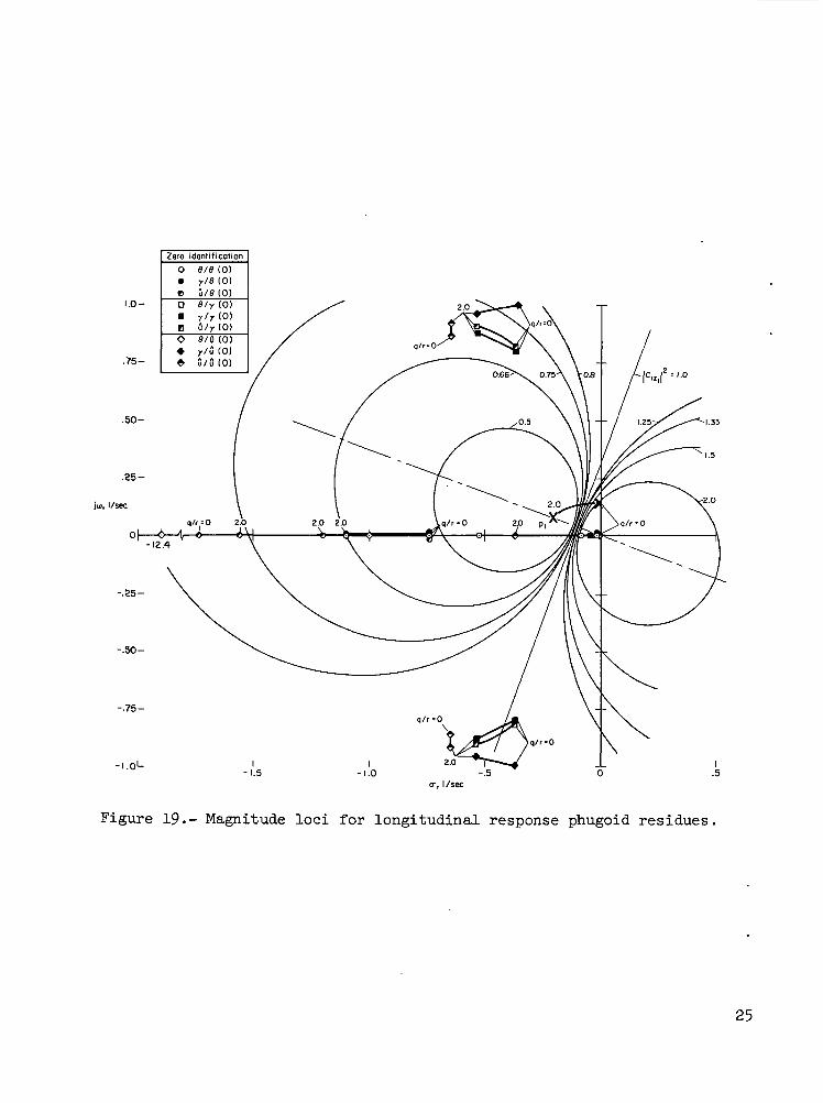
The aircraft system has three controls and three states of particularinterest, resulting in nine separate responses or transfer functions to beconsidered. Time histories of these states and controls for q/r values of 0and 2.0 are shown in figures 1^ through 17- The quantity y is also plottedto show the load factor. There are considerable changes in the time historieswith increasing q/r. Figures 18 through 20 show the loci required for theapplication of this method. Figure 18 shows the poles and zeros for all thevarious transfer functions for q/r = 0 and 2.0. In addition, the phase lociare drawn for q/r = 2.0 for both Pj_ = Pi and p^ = pa- Figure 19 shows thepoles and zeros, but also includes the magnitude loci associated with the

Se, rod

100 BT, % thrust

8F, rod

I10

I20

t, sec

I30

I40

Figure lU.- Transient responses due toinitial conditions of original sys-tem (q/r = 0); (a) in 9, (b) in y:(c) in u.

Figure 15-- Transient responses ofthe state and control variables ofthe regulated system (q/r = 2.0)due to initial condition in 9.

22

Figure l6.- Transient responses of the state and control variablesof the regulated system (q/r = 2.0) due to initial condition in y-

i.Op

-.5

SF, rod

Figure 17-- Transient responses of the state and control variablesof the regulated system (q/r = 2.0) due to initial condition in u.

23

1.0-

.75-

.50-

.25-

-.25-

5,I/sec

-.50-

-.75 L-1.5

Figure 18.- Phase loci for longitudinal response residues.

phugoid residues again for q/r =2.0. Figure 20 is similar to 19, with themagnitude loci drawn for the short-period residues . A number of the rootschange only slightly with q/r, and some change very similarly for severaltransfer functions.

In deriving the time vectors (or residues) by means of figures 18 through20, we use as an example the transfer function y/u(0) for q/r = 0, which hasa second-order numerator and a fourth-order denominator.. As shown earlier,the time vector of the short-period mode Y3» for instance, will be determined

3zfrom the residue 03 (at ps), which in turn consists of the product of Cand C3p (eq. (6)). The phase of C3z,<£3z is determined from p3 and z\ asindicated in figure 2l(a), which shows the appropriate poles and zerosextracted from figure 18. The conjugate zero Z2 does not need to be includedfor this plot. The quantity C3Z = c\ •which is abstracted from figure 20, usingr Q ™ and

process,

is obtained from figure 2l(b),p3 and z1}z2. These quantities,

|C3Z|, are then combined and plotted in figure 22 as C,shown in figure 2l(c) and (d), is used to derive jJ3^3z-

6-function input•"•Note that PsC3p or psC3 is used due to theinstead of a step input .

A similarThe phase

u(0)

1.0-

.75-

-.25-

-.50-

-.75-

-1.5 -1.0 .5a-, I/sec

Figure 19.- Magnitude loci for longitudinal response phugoid residues.

1.0-

.75-

-.25-

-.50-

-.75-

-1.5a, I/sec

Figure 20.- Magnitude loci for longitudinal response short-period residues,

26

(a

Figure 21.- (a) Phase locus and (b)magnitude loci for C3Z of the

transfer function y/u(0); q/r = 0.

Figure 21.- (c) Phase locus and (d)magnitude loci -for P3C3p of the

transfer function y/u(0); q/r = 0.

of PsCgp, denoted as <P3p in figure 22, is obtained by using pj instead of

zj (fig. 2l(c)). The angle of ir/2 must be added due to the contribution ofpit, the conjugate pole of ps, and the sign has to be changed (eq. (22)). Themagnitude of P3C3p is given by the product of jpsl and |C3p| = I/(GI '02*03)

which in turn is obtained from figure 2l(d), using all poles pi through pi+.Again, phase and magnitude are combined to plot psCs in figure 22.

for the time vector yi are obtainedThe quantities Clz andsimilarly using pi instead of

27

Pl-Cip

Figure 22.- The time vector construetion from the residue quantities.

im With PiCi (paCa) determined,the actual time vectors yit = 0 (fig. 22) are two times(psCs). This same process is used tcdetermine all the time vectors shownin the subsequent figures.

In the following, the timeresponses of the state components 6,Y, and u due to initial conditionsin the same states are discussedseparately, referring to figures 18through 20. The time histories ofthe controls could be discussed inthe same way.

6/e(0)—The attitude is the maincontrol variable in the longitudinalmotion of aircraft. The requirementis to reduce the initial attitudeerror in a rapid, well-damped mannerto zero. Without any control(q/r = 0), the time response behaviorof the attitude due to initial dis-placement shows large overshoot andvery little damping of the low-frequency mode, the phugoid (see

fig. lU), whereas for optimal control with respect to the chosen performanceindex and increasing q/r the desired behavior can be achieved, as shown infigure 15.

There are three real zeros but the overall tendencies in the change ofthe time response due to increasing q/r are caused mainly by the shift ofthe phugoid poles to higher damping and lower frequency. This shift willaffect all time responses, because the poles are the same for all transferfunctions for a given q/r. Therefore, for all transfer functions, there willbe the tendency for Cj, the phugoid mode residue or half of the time vector9j at t = 0, to shift its phase into the imaginary axis (fig. 23), as thephugoid poles approach the real axis of the root plane. (A similar effectwill occur for other transfer functions.) Because there is almost no changein the short-period poles with increasing q/r (also common for all transferfunctions), the location of the zeros with respect to the phugoid poles deter-mines how far the phase shift in 6j will go and what change in magnitude ofthat residue will occur.

As can be seen from figures 18 and 19, 1/Cp increases mainly in magni-tude and GIZ in phase with higher values of q/r. The phase shift ischiefly due to the shift of the phugoid poles in relation to the zero that is'closest to the origin. The change in the phase contribution of that zeroamounts to almost Tr/2 in the range of q/r from 0 through 2.0. Althoughthere are also changes taking place due to the zero farthest from the origin,

28

Figure 23.- Time vectors for thetransient response of 6/9(0) withq/r = 0 and 2.0.

that zero has little effect on eitherthe phase or magnitude of C1Z. Thus,the tendency in C1Z is simply.

q/r=o obtained by watching only the rela-q/r = 2.o tive location of the phugoid poles

and the zero close to the origin.With respect to 83 or C3 (the resi-due of the short-period mode), thechange in C3p is due to the phugoidshift and the change in C3Z is dueto the shift of the zero far from the •origin. These are opposing changes,such that the total change in 03 israther small.

The conclusion is that theeffect of the phugoid mode is con-siderably reduced by the large phaseshift in 9i toward the imaginary

axis and the high phugoid damping. On the other hand, choosing a well-dampedlocation for the phugoid and fixing one of the zeros, a given range of theClz-phase loci can be assigned to the location of the remaining zeros toachieve the desired behavior.

Y/Q(0) and u/Q(0)—Although suppression (decoupling) of the responses inthe flight-path angle y and the speed u due to initial displacement in theattitude might be desired, a certain amount of temporary displacement in bothy and u is required to avoid excessive costs in the controls. That is, avery effective lift control would be needed, with simultaneous speed control,to compensate for the initial lift change due to 9(0).

As can be seen from figures lU and 15, at least some improvement is made,particularly in the speed response, by minimizing the previously describedperformance index. Again, the main reason is the shift of the phugoid polestoward the real axis of the root plane, which leads to high damping and fixesthe phase of yj and UJ close to the imaginary axis for both the y and uresponse (fig. 2k).

To determine the actual phase of y^ and Y3> one can make use of theresults obtained by examining the zeros for 9/9(0) that are located in closevicinity to both existing zeros of y/9(0). Therefore, the phase differencebetween the residues of the responses in attitude and flight-path angle iscaused by the phase effect of the medium zero of 9/9(0). Because this zerodoes not change with q/r, the phase difference between the residues of9/9(0) and y/6(0) is also independent of q/r.

Response due to y(0) 0—As shown in figure 17 9 the response to an ini-tial displacement in the flight-path angle is good for the case of q/r =2.0.The flight-path angle itself settles down to small values very soon withoutevident oscillations, and the coupled motion in pitch and speed is almost neg-ligible. Also, the load factor due to the rate of change of the flight-path

29

X, <t=0)

fl,(t=0)

9,0=0)

•q/r = 0

•q/r =2.0

u,(t = 0)

fl|(t=0)

Im

••Re ••Re

32(t=0).-••Re

Figure 2k. - Time vectors for transient Figure 25.- Time vectors for trans-responses of Y/9(0) ancl u/6(o) ient responses of e/yCo), Y/Y(O)>with q/r = 0 and 2.0. and u/y(0) with q/r = 0 and 2.0.

angle does not appear to yield too high values . The plot of the time vectorsof the response in 9 is shown as part of figure 25. The short-period vectoris phased with respect to the phugoid vector such that. while rotating andbefore decaying, their real parts almost cancel, resulting in low coupling"between 9 and y(0) • This configuration of the vectors thus shows a highlydecoupled transfer function, and a similar configuration would be desirablefor other transfer functions. Comparing this configuration with that ofy/9(0) (fig. 2U), for instance, a smaller phase shift for Y3 vould produceless coupling. This could be obtained by locating the zeros on the corre-sponding phase locus curve. These phase values are easily obtained from fig-ure 25 since only one zero is involved in the 9/Y(0) response.

The pair of conjugate complex zeros of Y/Y(O) is almost coincident withthe zeros of U/Y(O) and Y/U (0). Thus, the difference in the behavior ofthese later two in comparison to Y/Y(O) is given by the real zero of Y/Y(^)>which again is almost independent of q/r. Observing the magnitude ratio

• between the residues Yi an<i YS in figure 25, one can see that increasing q/rresults in a high gain for YI relative to Y3» which gives a very slow long-term dynamic behavior.

Response due to u(0) ^ 0 — According to figure IT, the direct response inthe speed again appears satisfactory for moderate values of q/r. There is nofast response required for the speed so long as the initial error returns to

30

Im

••Re

Sj(t=0)|LX8|(t=0)

-••Re

X3(t=0)

Im

q/r=0

q/r= 2.0

u,(t=0)

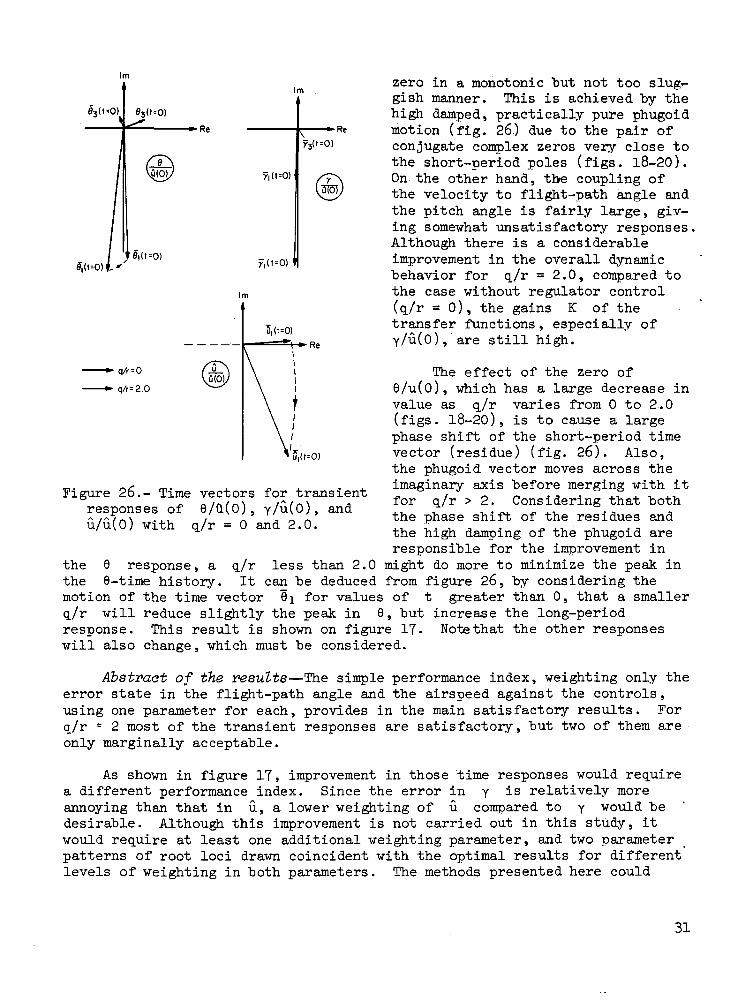
zero in a monotonic but not too slug-gish manner. This is achieved by thehigh damped, practically pure phugoidmotion (fig. 26) due to the pair ofconjugate complex zeros very close tothe short-period poles (figs. 18-20).On the other hand, the coupling ofthe velocity to flight-path angle andthe pitch angle is fairly large, giv-ing somewhat unsatisfactory responses.Although there is a considerableimprovement in the overall dynamicbehavior for q/r =2.0, compared tothe case without regulator control(q/r =0), the gains K of thetransfer functions, especially ofY/u(0), are still high.

u,(t=0)

Figure 26.- Time vectors for transientresponses of 9/u(0), y/u(0)»u/u(0) with q/r = 0 and 2.0.

The effect of the zero of6/u(0), which has a large decrease invalue as q/r varies from 0 to 2.0(figs. 18-20), is to cause a largephase shift of the short-period timevector (residue) (fig. 26). Also,the phugoid vector moves across theimaginary axis before merging with itfor q/r > 2. Considering that boththe phase shift of the residues andthe high damping of the phugoid areresponsible for the improvement in

the 6 response, a q/r less than 2.0 might do more to minimize the peak inthe 6-time history. It can be deduced from figure 26, by considering themotion of the time vector 61 for values of t greater than 0, that a smallerq/r will reduce slightly the peak in 6, but increase the long-periodresponse. This result is shown on figure IT- Note that the other responseswill also change, which must be considered.

Abstract of the results—The simple performance index, weighting only theerror state in the flight-path angle and the airspeed against the controls,using one parameter for each, provides in the main satisfactory results. Forq/r * 2 most of the transient responses are satisfactory, but two of them areonly marginally acceptable.

As shown in figure 17, improvement in those time responses would requirea different performance index. Since the error in y is relatively moreannoying than that in u, a lower weighting of u compared to y would bedesirable. Although this improvement is not carried out in this study, itwould require at least one additional weighting parameter, and two parameterpatterns of root loci drawn coincident with the optimal results for differentlevels of weighting in both parameters. The methods presented here could

31

still be used to aid in the determination of the elements of q. and r thatwould give the desired time responses.

CONCLUDING REMARKS

Two methods are described that provide geometrical insight into theeffect of the zeros of transfer functions as well as poles, on the correspond-ing time histories. The main advantage of these methods lies in their simplic-ity compared to other available procedures. They differ in their limitations,which are essentially those on the possible regions of the system polelocations.

The first method, which uses the geometrical interpretation of the resi-dues, loses much of its power if the poles become real, while the othermethod is restricted to certain separations of the poles, regardless ofwhether they are real or conjugate complex. In almost all cases, at least oneof the methods can be used effectively. This is especially true when appliedto aircraft transfer functions, as shown in the discussion of optimal regula-tor control for the longitudinal motion.

Both methods are developed for the type of transfer function with fourpoles and two zeros along with an extension to three zeros. Further extensionto allow for additional poles and zeros is possible, but will be verycomplicated.

The main use of the methods should be for analysis purposes. To inter-pret the effect of zero changes, the poles are assumed fixed, and changes inthe poles are discussed with the zeros unchanged. Thus, only if something isknown about the sensitivities of the pole locations due to zero changes andvice versa (ref. 8) can the methods be helpful in the synthesis process.

The methods are applied to a study of the longitudinal motion regulatorof an aircraft. The performance of this regulator system is studied using aparticular performance criterion with minor variations. This criterion mini-mizes the state errors effectively using only reasonable control effort.

Ames Research CenterNational Aeronautics and Space Administration

Moffett Field, Calif. 9^035, Feb. 3, 1972

32

APPENDIX A

EQUATION FOR THE MAGNITUDE LOCI OF C±z (TWO ZEROS)

The exact equation for the magnitude loci of C±z is simply derived fromequation (lU) "by substituting in the expressions for GI and c2 the values ofthe conjugate complex zeros, 21,2 = °z * <5uz:

c2

The coordinates of the pair of conjugate zeros generate fourth-order terms,such that the loci of ]C-;Z| in the root plane become higher order curves.For the special case of \C±z \ = 1» which might be of particular practicalinterest, equation (Al) reduces to

Ua3a. - 2a2(u>2 + 3a?) + Ua a. |p. |2 + Ua co2a. - 2(x)2(a? - to?) - |p. | k = 0Zl Zl 1 Z l ' ^ l 1 ZZ1 Z 1 1 'l 1

(A2)

From this equation, the simple formulas (l?) through (20) are derived forspecific points on that curve by substituting the specific values for az or0) .z

For a pair of real zeros, equation (A2) changes to

. - 2o2(u>2 + 3a?) + **a a. |p. |2 - Ua w2a. + 2^2(a2 - a)2) -z i z i i z i ' - ^ i 1 z z i z i i

(A3)

33

APPENDIX B

ENCIRCLING OF ZERO REGIONS FOR GIVEN VALUES OF |C.iz'

Practicable approximations can be made to encircle zero regions for givenvalues of \V±z\ rather than to define the exact loci curves. This appendixgives some further details on those approximations.

According to equations (15) and (l6) for the loci circles of c^ and 02,figure 27 illustrates the relation betveen the location of the center pointsof those circles and the corresponding values of GI and C2- It shows that onthe string of center points of the c^ circles, the corresponding value of GIis

= 1 + - >n

(Bl)

if the center point lies at a distance n|p.| downward from the origin and

c = 1 - < 11 n(B2)

if the center point lies n|pi| upward from the origin. The centers of theC2 circles are symmetrical about the real axis with the corresponding c^centers.

Figure 27.- Relation between values ofci,C2 and the location of the locicenter points.

In looking for the intersectionsbetween cj and C2 circles, it isevident that not all GI circlesintersect a particular C2 circle andvice versa. Therefore, consideringonly the upper half of the root planefor symmetry reasons, there are threeregions divided by the straight-lineloci of G! = 1 and C2 = 1 (fig. 7),such that (l) region I includes theintersections possible between thecircles of c^ < 1 and c2 > 1, (2)region II includes the intersectionspossible between the circles ofG! > 1 and c2 > 1, and (3) region IIIincludes the intersections possiblebetween the circles of c^ < 1 andc2 < 1. Encirclement of zero loca-tion areas due to certain values of\C±Z\ is given below for eachregion.

Region I

If one considers a possible intersection between circles of c^ < 1. andC2 > 1 (n > 1, m > 0), the corresponding magnitude of C can be writtenwith use of equation

|Ciz |2. 1-1 1+11 I nM m (B3)

or as an explicit relation for m as a function of n with the parameter|c. | , as illustrated in figure 28,1Z

m = n - 1

(|Ciz|2 -1) n + 1

Figure 28.- |Cj_z| as function ofm and n (region I).

plane. The upper limit for m and n

The figure shows that for values of|C Z| distinctly smaller (larger)than 1, n (m) does not go over a cer-tain small value. Therefore, the:range of circles in GI (02) corre-sponding to those |Ciz| values isalso very limited. Thus, for a cer-tain value of |Cj_z|, the correspond-ing zeros and all those for'smaller(greater) values of |Ciz| must liewithin the largest possible circlefor GI (co), which is that forcl = |Ciz|(c2 = |ciz|) (see fig. 7).The range of possible combinations ofm and. n is not only limited as shownin figure 28; for higher values of nand m, the circles might not inter-sect such that no locus point for|C'iz! can be defined in the root

can be easily described by the followingcondition, which depends on the location of the pole

= 20).

I Pi(B5)

Figure 28 itself is valid for all locations of

Region II

Within this region the relation between the location of the circles for> 1 and c 2 > l ( n > 0 , m > 0 ) and \C±Z\ itself is

35

or

= 1 + - 1 + - > 1

m = n + 1

( I c . z l 2 - l ) n -

(B6)

(BT)

Figure 29.- |Cj.2 | as a functionof m and n (region II)..

|C iz|=const

Figure 30.- Approximate region for(C^zl locus (region II).

as illustrated in figure 29, whichagain is independent of the locationof the pole p^. The curves are sym-metrical with respect to the straightline m = n. Calling n = n* andm = m* for the point m = n , for eachcurve it can be stated that for alln > n* (lower half of the curve)m < m* , and also for all m > m*(upper half of the curve) n < n*.Therefore , each point on the lowerhalf of the curve represents a zerolocation that must "be inside the G£circle given by m = n* and outsidethe GI circle given by n = n*. Acorresponding remark can be given forthe upper part of the curve . Thus ,the loci for |C Z| can be locatedin the root plane as: .(l) beingwithin the union but outside theintersection of the circles for GIand C2 corresponding to n =m = m*, respectively, where

= * and

= c2 = |Clz1/2

and (2) intersecting the real axis atthe same points, where the circles of(l) are intersecting (fig. 30).

From equation (B6), it followsthat

n* = m* = (B8)- 1

As in region I, there is an upperlimit for m and n, dependent onwhich is defined as follows:

36

= 20).1

Ipil (B9)

This condition can be used, of course, for further encircling.

Region III

Analogous to the approximation applied to region II, for region III, with< 1 and c2 < 1 (n > 1, m > l),

or

.iz

m =

n

1 - n

( |C. I2 - l)n + 11 iz '

(BIO)

(Bll)

= 0.64

Figure 31.- |Ciz| as a function ofm and n (region III).

which is illustrated in figure 31.Again, the loci for |Cj_z| in theroot plane can be located as withinthe union but outside the intersec-tion of the circles of cj and c2corresponding to n = n* and m = m*,respectively, with

= c2 = 'IZ

and

n* = m* =

(B12)

(B13)1 - Ciz i

The upper limits on n and m in figure 31, dependent on the location of p^are given by

c2| = 2 (BlU)

I Pi

37

REFERENCES

1. McRuer, D. T. ; Ashkenas, I. L.; and Pass, H. R.: Analysis of MultiloopVehicular Control Systems. ASD-TDR-62-101 , 196U.

2. Brockhaus, R.: Uber die Verkopplung und den Einfluss von Allpasseigen-schaften in speziellen Mehrgrb'ssensystemen am Beispiel de'r Regelung derFlugzeuglangsbewegung im Landeanflug. Deutsche Forschungsanstalt furLuft-und Raumfahrt, DLR-FB 67-71*, 196?.

3. Onken, R.: Erweiterung der Zeitvektormethode auf Bevegungsgleichungen mitreellen Wurzeln und die Anwendung des Verfahrens auf Probleme derFlugregelung. Jahrbuch der Deutschen Gesellschraft ftlr Luft-undRaumfahrt, 1969.

H. Doetsch, Karl H.: The Time Vector Method for Stability" Investigations.RAE TR Aero 2U95 (ARC 16275), ARC R. & M. 29^5, 1953.

5. Onken, R.; and Leyendecker, H.: Anwendung der Zeitvektormethode zurInterpretation und Optimalen Festlegung der ZShlerwurzeln von Uber-tragungsfunktionen. Published in forthcoming issue of "Zeitschrift ftlrRegelungstechnik."

6. Rynaski, E. G. ; and Whitbeck, R. F.: The Theory and Application of LinearOptimal Control. AFFDL-TR-65-28, 1966.

7. Athans, Michael; and Falb, Peter L.: Optimal Control. McGraw-Hill BookCo., 1966.

8. McRuer, D. T.; and Stapleford, R. L.: Sensitivity and Modal Response forSingle-Loop and Multiloop Systems. ASD-TDR-62-812, 1963.

38 NASA-Langley, 1972 2 A-

AERONAUTICS

; WASHINGTON. D,C. (20546

BUSI

?C;-<>,LTY FOR PRIVAT

POSTAGE!

FIRST CLASS MAIL

NASA

POSTMASTER: f UadeUvfcaWe(Section 158I 4. ." POS^U Manua/ , .

"ffTjfie iievonaiitifal and if ace actii^iesconducted so as to contribute . . , to theedge of phenomena in the atmosphc'shall provide for ti » j/ practicable i;:QJ'information concerning its activities a

t —NATIONAL AERONAUT

the c ill beKpans, :M knottd-space, "the Administration

' appropriate d* -:ttion

NASA SCIENTIFIC AND TECHNICAL i>U [QNS

I TECHNICAL REPORTS; Scientific and:;technical information considered important,complete, and a; lasting contribution to existing

Information Jess broad; of importance is |knowledge, 1tiiSn to existtr

IGAL MEMOKANDUMS:

'iminary data, security classifies^

)R KEipORT^: Scientific amimation generated under a NASAnt and considered an importanti existing knowledge.. , •

TECHNICAL TRANSLATIONS: Informationpublished in a foreign language consideredto merit NASA distribution in English.

SPECIAL PUBLICATIONS: InformationJderived from or of value to NASA activities.Publications include conference proceedings, ,:,m6n§graphs, data compilations, handfaooks,so|!rc«boofcs, and special bibliographies.

TECHNOLOGY UTILIZATIONPUBLICATIONS; Iniorrnation on technologyused by NASA that may be of particularinterest in commercial and other non-aerospaceapplications. Publications include Tech Briefs,?Technology Utilization Reports andTechnology Surveys. ';

Details on the availability of (Aese publications may be obtained from:

SCIENTIFIC AND TECHNICAL INFORMATION OFFICE

NATIONAL AERONAUTICS AND SPACE ADMINISTRATIpNWashington, D.C 20546