Approximate computation and implicit Approximate computation and implicit regularization in large-scale data analysisregularization in large-scale data analysis

Michael W. Mahoney

Stanford University

Sept 2011

(For more info, see: http://cs.stanford.edu/people/mmahoney)

Motivating observation

Theory of NP-completeness is a very useful theory• captures qualitative notion of “fast,” provides an qualitative guidance to how algorithms perform in practice, etc.

• LP, simplex, ellipsoid, etc. - the “exception that proves the rule”

Theory of Approximation Algorithms is NOT analogously useful• (at least for many machine learning and data analysis problems)

• bounds very weak; can’t get constants; dependence on parameters not qualitatively right; does not provide qualitative guidance w.r.t. practice; usually want a vector/graph achieving optimum, bu don’t care about the particular vector/graph; etc.

Start with the conclusions

• Modern theory of approximation algorithms is often NOT a useful theory for many large-scale data analysis problem

• Approximation algorithms and heuristics often implicitly perform regularization, leading to “more robust” or “better” solutions

• Can characterize the regularization properties implicit in worst-case approximation algorithms

Take-home message: Solutions of approximation algorithms don’t need to be something we “settle for,” since they can be “better” than the solution to the original intractable problem

Algorithmic vs. Statistical Perspectives

Computer Scientists • Data: are a record of everything that happened. • Goal: process the data to find interesting patterns and associations.• Methodology: Develop approximation algorithms under different models of data access since the goal is typically computationally hard.

Statisticians (and Natural Scientists)• Data: are a particular random instantiation of an underlying process describing unobserved patterns in the world.• Goal: is to extract information about the world from noisy data.• Methodology: Make inferences (perhaps about unseen events) by positing a model that describes the random variability of the data around the deterministic model.

Lambert (2000)

Statistical regularization (1 of 2)

Regularization in statistics, ML, and data analysis

• arose in integral equation theory to “solve” ill-posed problems

• computes a better or more “robust” solution, so better inference

• involves making (explicitly or implicitly) assumptions about the data

• provides a trade-off between “solution quality” versus “solution niceness”

• often, heuristic approximation have regularization properties as a “side effect”

Statistical regularization (2 of 2)Usually implemented in 2 steps:

• add a norm constraint (or “geometric capacity control function”) g(x) to objective function f(x)

• solve the modified optimization problem

x’ = argminx f(x) + g(x)

Often, this is a “harder” problem, e.g., L1-regularized L2-regression

x’ = argminx ||Ax-b||2 + ||x||1

Two main results

Big question: Can we formalize the notion that/when approximate computation can implicitly lead to “better” or “more regular” solutions than exact computation?

Approximate first nontrivial eigenvector of Laplacian• Three random-walk-based procedures (heat kernel, PageRank, truncated lazy random walk) are implicitly solving a regularized optimization exactly!

Spectral versus flow-based approximation algorithms for graph partitioning• Theory suggests each should regularize in different ways, and empirical results agree!

Approximating the top eigenvector

Basic idea: Given a Laplacian matrix A,

• Power method starts with v0, and iteratively computes

vt+1 = Avt / ||Avt||2 .

• Then, vt = i it vi -> v1 .

• If we truncate after (say) 3 or 10 iterations, still have some mixing from other eigen-directions

What objective does the exact eigenvector optimize?• Rayleigh quotient R(A,x) = xTAx /xTx, for a vector x.

• But can also express this as an SDP, for a SPSD matrix X.

• (We will put regularization on this SDP!)

Views of approximate spectral methods

Three common procedures (L=Laplacian, and M=r.w. matrix):

• Heat Kernel:

• PageRank:

• q-step Lazy Random Walk:

Ques: Do these “approximation procedures” exactly optimizing some regularized objective?

Two versions of spectral partitioning

VP:

R-VP:

Two versions of spectral partitioning

VP: SDP:

R-SDP:

R-VP:

A simple theorem Modification of the usual SDP form of spectral to have regularization (but, on the matrix X, not the vector x).

Mahoney and Orecchia (2010)

Three simple corollariesFH(X) = Tr(X log X) - Tr(X) (i.e., generalized entropy)

gives scaled Heat Kernel matrix, with t =

FD(X) = -logdet(X) (i.e., Log-determinant)

gives scaled PageRank matrix, with t ~

Fp(X) = (1/p)||X||pp (i.e., matrix p-norm, for p>1)

gives Truncated Lazy Random Walk, with ~

Answer: These “approximation procedures” compute regularized versions of the Fiedler vector exactly!

Graph partitioning

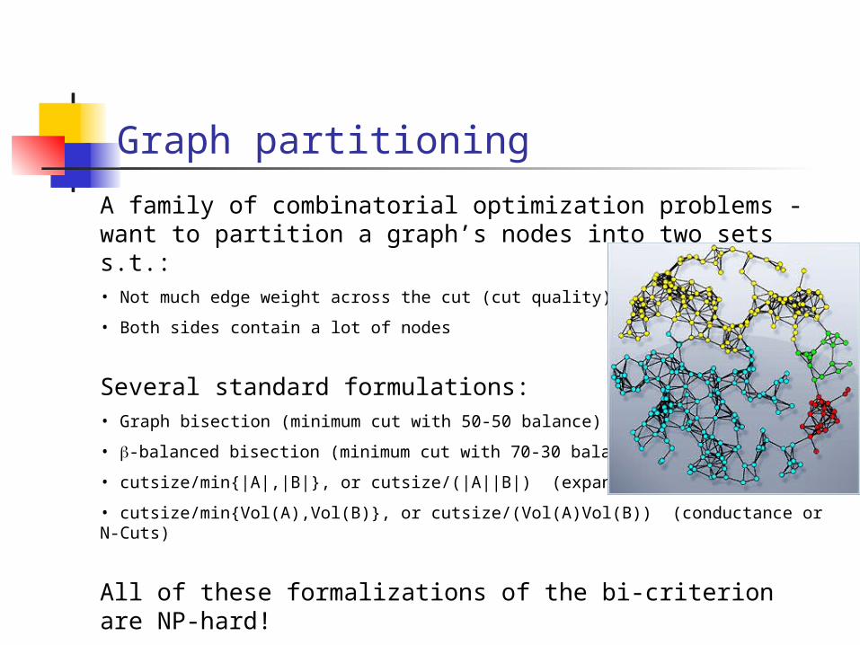
A family of combinatorial optimization problems - want to partition a graph’s nodes into two sets s.t.:• Not much edge weight across the cut (cut quality)

• Both sides contain a lot of nodes

Several standard formulations:• Graph bisection (minimum cut with 50-50 balance)

• -balanced bisection (minimum cut with 70-30 balance)

• cutsize/min{|A|,|B|}, or cutsize/(|A||B|) (expansion)

• cutsize/min{Vol(A),Vol(B)}, or cutsize/(Vol(A)Vol(B)) (conductance or N-Cuts)

All of these formalizations of the bi-criterion are NP-hard!

The “lay of the land”

Spectral methods* - compute eigenvectors of associated matrices

Local improvement - easily get trapped in local minima, but can be used to clean up other cuts

Multi-resolution - view (typically space-like graphs) at multiple size scales

Flow-based methods* - single-commodity or multi-commodity version of max-flow-min-cut ideas

*Comes with strong underlying theory to guide heuristics.

Comparison of “spectral” versus “flow”

Spectral:

• Compute an eigenvector

• “Quadratic” worst-case bounds

• Worst-case achieved -- on “long stringy” graphs

• Worse-case is “local” property

• Embeds you on a line (or Kn)

Flow:

• Compute a LP

• O(log n) worst-case bounds

• Worst-case achieved -- on expanders

• Worst case is “global” property

• Embeds you in L1

Two methods -- complementary strengths and weaknesses

• What we compute is determined at least as much by as the approximation algorithm as by objective function.

Explicit versus implicit geometry

Explicitly-imposed geometry

• Traditional regularization uses explicit norm constraint to make sure solution vector is “small” and not-too-complex

(X,d) (X’,d’)

x

y

d(x,y) f

f(x)

f(y)

Implicitly-imposed geometry

• Approximation algorithms implicitly embed the data in a “nice” metric/geometric place and then round the solution.

Regularized and non-regularized communities

• Metis+MQI - a Flow-based method (red) gives sets with better conductance.

• Local Spectral (blue) gives tighter and more well-rounded sets.

External/internal conductance

External/internal conductance

Diameter of the cluster

Diameter of the cluster

Conductance of bounding cutConductance of bounding cut

Local Spectral

Connected

Disconnected

Low

er is g

ood

Conclusions

• Modern theory of approximation algorithms is often NOT a useful theory for many large-scale data analysis problem

• Approximation algorithms and heuristics often implicitly perform regularization, leading to “more robust” or “better” solutions

• Can characterize the regularization properties implicit in worst-case approximation algorithms

Take-home message: Solutions of approximation algorithms don’t need to be something we “settle for,” since they can be “better” than the solution to the original intractable problem