Approximate Bayesian Inference in SpatialGeneralized Linear Mixed Models

Jo Eidsvik, Sara Martino and Havard Rue

Department of Mathematical Sciences, NTNU, Norway.

Address: Department of Mathematical Sciences, NTNU, 7491 Trondheim, NORWAY.

Corresponding author: Jo Eidsvik (joeid@math.ntnu.no)

Jo Eidsvik (joeid@math.ntnu.no) is Associate Professor;

Sara Martino (martino@math.ntnu.no) is PhD student;

Havard Rue (hrue@math.ntnu.no) is Professor.

Affiliation of all authors:

Department of Mathematical Sciences, NTNU, 7491 Trondheim, Norway.

1

ABSTRACT

In this paper we propose fast approximate methods for computing posterior marginals in spatial

generalized linear mixed models. We consider the common geostatistical special case with a high

dimensional latent spatial variable and observations at only a few known registration sites. Our

methods of inference are deterministic, using no random sampling.

We present two methods of approximate inference. The first is very fast to compute and via

examples we find that this approximation is ’practically sufficient’. By this expression we mean

that the results obtained by this approximate method do not show any bias or dispersion effects

that might affect decision making. The other approximation is an improved version of the first

one, and via examples we demonstrate that the inferred posterior approximations of this improved

version are ’practically exact’. By this expression we mean that one would have to run Markov

chain Monte Carlo simulations for longer than is typically done to detect any indications of bias or

dispersion error effects in the approximate results.

The two methods of approximate inference can help to expand the scope of geostatistical mod-

els, for instance in the context of model choice, model assessment, and sampling design. The

approximations take seconds of CPU time, in sharp contrast to overnight Markov chain Monte

Carlo runs for solving these types of problems. Our approach to approximate inference could

easily be part of standard softwares.

KEYWORDS: Approximate inference, spatial GLM, circulant covariance matrix, Newton-Raphson,

MCMC.

2

1. INTRODUCTION

Several statistical problems include the analysis of data acquired at various spatial locations.

In Bayesian geostatistical modeling one typically treats these data as indirect measurements of a

smooth latent spatial variable, with priors for the parameters of the model. Among the popular

applications are geophysics, mining, meteorology and disease mapping, see e.g. Cressie (1991),

Diggle, Tawn and Moyeed (1998) and Banerjee, Carlin and Gelfand (2004). For Bayesian analysis

of spatial data there are mainly two objectives; i) inference of model parameters, for example the

standard deviation (or precision) and the range of the latent spatial variable, and ii) prediction of

the latent variable at any spatial location.

One topic that has received much attention lately is inference and prediction for the spatial

generalized linear mixed model (GLMM), see e.g. Diggle et al. (1998) and Christensen, Roberts

and Skold (2006). This common model can briefly be described as follows: Let x represent a latent

spatial variable on a grid of n regularly spaced gridnodes on a two dimensional lattice. Suppose

that x has a stationary Gaussian prior distribution specified by some covariance model parameters

θ. Suppose next that observations y are made at k of the n nodes. These observations are modeled

as an exponential family distribution with parameters given by the latent variable x at the sites

where the data is acquired. Typical examples of this model include Poisson counts or binomial

proportions registrered at some known locations in space, with the objective of predicting the

underlying intensity or (log odds) risk surface across the spatial domain of interest, and inferring

model parameters. The most common case is probably the situation where one wants to predict

across a large spatial domain, but only a few locations register data, i.e. n � k. For example,

this situation occurs in spatial data acquisition for weather forecasting (Gel, Raftery and Gneiting

2004) and in reserve site selection for predicting the presence of a certain type of species (Polasky

and Solow 2001). Both examples in Diggle et al. (1998) are also of this type with n � k.

Bayesian analysis of spatial GLMMs have been considered difficult since the spatial problem is

of high dimension and because of the lack of closed form solutions. The current state of the art is to

generate realizations of parameter θ and latent spatial variable x using Markov chain Monte Carlo

(MCMC) algorithms. Since MCMC algorithms have grown mature over the last few decades,

3

see e.g. Robert and Casella (2004), there is a number of fit-for-purpose algorithmic techniques

for doing iterative Markov chain updates. Some of these algorithms are more relevant for spatial

GLMMs (Diggle et al. 2003), but problems remain with convergence and mixing properties

of the Markov chain, which in some cases are remarkably slow. Because of these challenges

fast inference methods suitable for special cases are needed, possibly avoiding the problems with

sampling methods.

The main contribution of this paper is a new method for approximate inference in spatial

GLMMs with n � k. In particular, this paper provides a recipe for fast approximate Bayesian

inference using the marginals π(θ|y) and π(xj|y), j = 1, . . . , n, i.e. the marginal posterior density

of the model parameters and the marginal posterior density of the latent variable at any spatial loca-

tion. We also illustrate how the marginal likelihood π(y) can be estimated within our framework.

The examples show that the fast approximate method is ’practically sufficient’. By this expression

we mean that results obtained by the approximate method and tedious Monte Carlo algorithms

are hard to distinguish and that for most practical decision purposes the approximate method ob-

tains in almost no time what the Monte Carlo approach would need much computation time to

achieve. This result is important for general practitioners of geostatistics that can possibly avoid

iterative Monte Carlo simulations which are hard to monitor, and rather do the direct calculation

at almost no computational cost. Moreover, the approximate method could easily be incorporated

in standard softwares. Fast approximate inference for this model can further help to expand the

scope of geostatistical modeling. Possible applications include geostatistical design (Diggle and

Lophaven 2006), and model choice (Clyde and George 2004) or model assessment (Johnson 2004)

in a geostatistical setting.

Another contribution of this paper is an improved approximation for spatial prediction, going

beyond our basic direct approximate solution. While the direct approximation uses the joint pos-

terior mode for x to do spatial prediction, the improved approximation splits the joint into the

marginal of xj and the conditional for the remaining spatial nodes. The improved version pro-

vides a natural correction to the direct approximation. Improvements become important at spatial

locations j where the direct approximation to π(xj|y, θ) or π(xj|y) is not sufficiently accurate,

4

typically spatial sites where there are lots of non-Gaussian data. In our examples we find that this

improved approximation is ’practically exact’. By this expression we mean that results obtained

by the approximate approach and tedious Monte Carlo algorithms are indistinguishable, and that it

is very hard to detect if small differences indicate limited run time in the Monte Carlo method or

slight bias in the improved approximate approach.

Other recent approaches to approximate inference for spatial generalized linear models include

Breslow and Clayton (1993) who studied penalized quasi likelihood, Ainsworth and Dean (2006)

who compared penalized quasi likelihood with a Bayesian solution based on MCMC computations,

and Rue and Martino (2006a) who used the Laplace approximation that we consider here, but with

a Gaussian Markov random field for the latent variable. The above references all used examples

where k is of the same order as n.

The outline is as follows: In Section 2 we define the special case of spatial GLMMs considered

in this paper. The proposed method of approximate inference and prediction is described in Section

3, while Section 4 uses the Rongelap radionuclide dataset as an example of this method. After

the ideas and results of the direct approximation have been presented, we describe the improved

approximation for spatial prediction in Section 5, and use the Lancashire infection dataset as an

example of this in Section 6. We discuss and conclude in Section 7. The computational aspects of

our methods are postponed to the Appendix.

2. SPATIAL GLMM

Let x = (x1, . . . , xn)′ represent the latent field on a regular grid of size n = n1n2, where n1 and

n2 are the grid sizes in the North and East directions. In an application with binomial proportions

data, the spatial variable x would denote the latent risk or log odds surface, while it would denote

the latent log intensity surface for Poisson count data. Suppose x has a stationary Gaussian prior

with π(x|θ, µ) = N [x; µ1n,Σ(θ)], where 1n denotes an n × 1 vector of ones, and Σ = Σ(θ)

is a positive definite, block circulant covariance matrix with θ indicating the model parameters.

For example, θ could include σ = pointwise standard deviation, and ν = spatial correlation range.

Block circulant covariance structure means that the n1×n2 grid is wrapped on a torus. As a simple

5

example of a covariance function we give the exponential defined by

Σh(σ, ν) = σ2 exp(−δh/ν), h =√

h21 + h2

2, (1)

where (h1, h2) are the (North, East) gridsteps between two nodes on the torus surface, while δ

specifies the spacing on the grid. Many others are possible, such as the Matern covariance function

which is often recommended, see e.g. Cressie (1991) and Stein (1999). We discuss this more

general class of covariance functions in the context of an application. The covariance function

imposes dependence in the latent variable, and in practice this means a smooth underlying risk

or intensity surface, as one could expect. A Bayesian view is taken here with priors π(µ) =

N(µ; β0, τ2) and π(θ) for the parameters. The µ mean parameter can then be integrated out to

obtain π(x|θ) = N(x; β, C), β = β01n and C = 1nτ 21′n + Σ, a block circulant matrix. Block

circulant covariance structure means that the fast Fourier transform can be used as an efficient

computational tool, see Appendix.

Suppose next that measurements yi, i = 1, . . . , k, are conditionally independent with likelihood

π(yi|xsi) = exp{[yixsi

− b(xsi)]/a(φ) + c(φ, yi)}, i = 1, . . . , k, (2)

where xs = (xs1, . . . , xsk

)′ = Ax and the k × n matrix A has entries

Aij = I(si = j) =

1 if si = j

0 else, i = 1, . . . , k, j = 1, . . . , n, (3)

i.e. si is the gridnode of measurement i. With n � k the matrix A consists mostly of 0 values, but

it has one 1 value for each row / observation. For the exponential family distribution in equation

(2) we have simple functional relationships for b(x) and a(φ). For example, the Poisson, Binomial

and Gaussian distributions can be defined by

Poisson Binomial Gaussian

b(x) m exp(x) m log[1 + exp(x)] x2/2

a(φ) 1 1 φ2

, (4)

where m is a fixed parameter and φ is a fixed standard deviation of the Gaussian likelihood

model. These relationships are commonly used in generalized linear models (McCullagh and

6

Nelder 1989). For example, Poisson is a case of log link function for count data, while the Bino-

mial likelihood is a case of logit link function for proportions. The model treated in this paper is

different from the standard GLMM setting because the data y are acquired at various spatial sites

and because of the spatially correlated latent variable x. Hence the term spatial GLMM.

3. APPROXIMATE INFERENCE AND PREDICTION

We will now outline our methods for fast approximate analysis of Bayesian spatial GLMMs

with n � k. The first step is to use a Gaussian approximation at the mode of the conditional

density π(x|y, θ). We next use this full conditional to approximate the densities of main interest;

π(θ|y) and π(xj|y). The marginal likelihood π(y) is also approximated. We have chosen to

postpone the technical details to the Appendix.

3.1 Gaussian approximation for π(x|y, θ) at the posterior mode

The full conditional density of the latent spatial variable is

π(x|y, θ) ∝ exp{−1

2x′C−1x + x′C−1β +

k∑

i=1

[yixsi− b(xsi

)]/a(φ)}. (5)

A Gaussian approximation to this density is constructed by linearizing the likelihood part of equa-

tion (5) at a fixed location x0s = Ax0. For each i = 1, . . . , k this involves

[yixsi− b(xsi

)] ≈ [yix0si− b(x0

si)] + (xsi

− x0si)[yi − b′(x0

si)] − 1

2(xsi

− x0si)2b′′(x0

si), (6)

where the first and second derivatives can be written in closed form using equation (4). Inserting

this into equation (5) gives a Gaussian approximation N [x; µx|y,θ(y, x0), V x|y,θ(x0)]. The

conditional covariance equals

V x|y,θ(x0) = C − CA′R−1AC, R = ACA′ + P , (7)

where P is diagonal with entries Pi,i = a(φ)/b′′(x0si), i = 1, . . . , k. The conditional mean is

µx|y,θ(y, x0) = [C−1 + A′P−1A]−1[C−1β + A′P−1z(y, x0s)],

= β + CA′R−1[z(y, x0s) − Aβ], (8)

7

where we use

zi(yi, x0si) = [yi − b′(x0

si) + x0

sib′′(x0

si)]/b′′(x0

si), i = 1, . . . , k. (9)

Rather than fitting a Gaussian approximation at any x0, the above process is iterated using

the Newton-Raphson algorithm. After a few iterations we have then fitted a Gaussian approxima-

tion π(x|y, θ) at the argument of the posterior mode denoted by mx|y,θ, see Appendix. These

Newton-Raphson calculations are similar to the traditional ones used for generalized linear mod-

els (McCullagh and Nelder 1989), but note that the dimension n of the latent variable x is large

here and regular optimization would often be impossible for spatial models, except in small sit-

uations such as a limited number of counties (Breslow and Clayton 1993). One contribution of

the current paper is to demonstrate that the Newton-Raphson optimization can be done in a fast

manner using benefits of the Fourier domain. The effective method applies to our special case with

n � k and stationary prior density for the latent variable. This indicates that large problems of

this common type can be handled with modest cost.

We remark some relevant features of the Gaussian approximation π(x|y, θ). The computa-

tional details of these remarks are presented in the Appendix.

• The latter expression in equation (8) involves the inversion of a k×k matrix R and is clearly

preferable in our case with n � k.

• Equation (8) is computed efficiently in the Fourier domain since C is block circulant.

• The Gaussian approximation π(x|y, θ) is evaluated using Bayes theorem and benefits of the

Fourier domain.

• Newton-Raphson optimization involves iterative calculation of equation (8) and is hence also

available in the Fourier domain.

The quality of the Gaussian approximation depends on the particular situation. Intuitively one

would expect it to be quite good since n � k and hence the smooth Gaussian prior has much

influence.

8

3.2 Parametric inference using π(θ|y)

The marginal density of model parameters θ is

π(θ|y) =π(y|x)π(x|θ)π(θ)

π(y)π(x|y, θ)∝ π(y|x)π(x|θ)π(θ)

π(x|y, θ), (10)

which is valid for any value of the spatial variable x, for example x = mx|y,θ, the argument at

the posterior mode for fixed θ. The challenging part of equation (10) is the denominator π(x|y, θ)

which is not available in closed form. We choose to approximate this denominator using the fitted

Gaussian density in Section 3.1. The approximate density for the model parameters is then

π(θ|y) ∝ π(y|x)π(x|θ)π(θ)

π(x|y, θ)

∣

∣

∣

∣

∣

x=mx|y,θ

. (11)

Equation (11) is the Laplace approximation, see e.g. Tierney and Kadane (1986) and Carlin and

Louis (2000). The relative error is O(k−3/2) (Tierney and Kadane 1986). Relative error is advan-

tageous, especially in the tails of the distribution. Equation (11) can be evaluated efficiently using

properties of the Gaussian approximation, see Appendix.

To calculate the approximation in equation (11) we first locate the mode of π(θ|y) and fit the

dispersion from the Hessian at this mode. In the relevant domain of the sample space for θ we

then evaluate equation (11) for a finite set of parameter values θl = (σl1 , νl2), l1 = 1, . . . , L1,

l2 = 1, . . . , L2, normalized so that

∑

l

∆σ∆νπ(θl|y) = ∆σ∆ν

L1∑

l1=1

L2∑

l2=1

π(σl1 , νl2 |y) = 1. (12)

In this equation ∆σ and ∆ν are the spacings in the defined grid for σ and ν values. The approximate

marginal densities are

π(σl1 |y) = ∆σ

L2∑

l2=1

π(σl1 , νl2|y), π(νl2 |y) = ∆ν

L1∑

l1=1

π(σl1 , νl2 |y). (13)

The density function π(θ|y) can also be approximated differently, for example by a parametric fit

to the density or by numerical quadrature (Press, Teukolsky, Vetterling and Flannery 1996). We

do not consider this here.

9

For the case with a Gaussian likelihood in equation (2) we can evaluate π(θ|y) exactly on the

grid of θ values (Diggle et al. 2003), whereas for the non-Gaussian case we merely obtain an

approximation π(θ|y) on this set of parameter values. Note that constructing π(θ|y) can be done

using only xs = Ax, i.e. latent values at the registration sites, but in this presentation we have

chosen to use the entire spatial variable x because this brings together the inference and prediction

steps.

3.3 Estimation of marginal likelihood π(y)

For assessing the statistical model one often uses the marginal likelihood π(y), see e.g. Hsiao,

Huang and Chang (2004). The marginal likelihood is given by

π(y) =π(y|x)π(x|θ)π(θ)

π(θ|y)π(x|y, θ). (14)

The denominator in equation (14) can be approximated using the Gaussian approximation for

latent variable and the approximate marginal for model parameters. These are both available.

The simplest way to evaluate the marginal likelihood is however to use the normalizing constant

required for computing the approximate density in equation (11) and (12). We denote this estimate

of the marginal likelihood by π(y). Efficient computation of the marginal likelihood becomes

important for example in model choice (Clyde and George 2004). For spatial models one natural

model check is related to the choice of covariance function. We demonstrate this in one of the

examples below.

3.4 Spatial prediction using π(xj|y)

For approximate Bayesian spatial prediction we use marginals π(xj|y) =∑

l π(xj|y, θl)π(θl|y),

j = 1, . . . , n. This is a mixture of Gaussian distibutions with the weights denoting the posterior

for each model parameter. The approximate marginal means become

µxj |y ≈∑

l

mxj |y,θl

π(θl|y), j = 1, . . . , n, (15)

10

where we pick element j of the joint conditional mode obtained at the last Newton-Raphson opti-

mization step. The approximate marginal variances are

Vxj |y ≈∑

l

Vxj |y,θl

π(θl|y) +∑

l

(mxj |y,θl

− µxj |y)2π(θl|y), j = 1, . . . , n, (16)

where Vxj |y,θ = V

xj |y,θ(mx|y,θ) denotes diagonal element j of the conditional covariance in

equation (7), evaluated at the argument of the posterior mode. For these variance terms we need to

calculate the diagonal entries of CA′R−1AC given by

(CA′R−1AC)jj =k

∑

i=1

k∑

i′=1

Cj,siR−1

ii′ Csi′ ,j, j = 1, . . . , n. (17)

3.5 Approximations as proposal distributions in Monte Carlo sampling

We now discuss Monte Carlo methods for checking the quality of the approximations. The

approximations are then used as proposals in a Metropolis–Hastings (MH) algorithm or in impor-

tance sampling.

Consider an independent proposal MH algorithm with proposed value x′ from the Gaussian

approximation π(x′|y, θ), keeping θ fixed. The proposal x′ is generated efficiently in the Fourier

domain, see Appendix. The acceptance rate becomes

min

{

1,[∏k

i=1 π(yi|x′si)]π(x′|θ)

[∏k

i=1 π(yi|xsi)]π(x|θ)

π(x|y, θ)

π(x′|y, θ)

}

, (18)

otherwise we keep the current value x in the Markov chain. The acceptance probability in equation

(18) can be evaluated using properties of the Gaussian approximation, see Appendix. This MH

scheme might be effective since large changes are proposed at every iteration, see e.g. Robert and

Casella (2004). Simultaneous MH updates of (x′, θ′) are also possible using the approximation

π(θ′|y) followed by π(x′|y, θ′), and then checking for acceptance.

One can alternatively use importance sampling (Shepard and Pitt 1997) based on the approx-

imations presented above. This is done by first generating xb, b = 1, . . . , B, independently from

π(x|y, θ). The B samples are next weighted based on the ratio of the posterior and the Gaussian

approximation. It is again possible to sample (xb, θb) using π(θb|y) followed by π(xb|y, θb) for

joint Monte Carlo estimation.

11

The Monte Carlo error of estimates based on B samples is additive and Op(B−1/2). The error

can thus be reduced by increasing the number of samples, but the additive nature might cause

problems in the tails of the distribution, especially compared to the relative error of the Laplace

approximation.

4. EXAMPLE OF APPROXIMATE INFERENCE

In this Section we redo one of the examples used in Diggle et al. (1998). The data are made

at only a few registration sites and the large latent spatial variable is modeled by a stationary prior

distribution. The dataset consists of k = 157 measurements of yi = radionuclide counts for various

time durations mi, i = 1, . . . , k. All 157 registration sites are displayed on the map in Figure 1.

The data are modeled as a spatial GLMM with a Poisson distribution in equation (2). The goal is

to assess the latent intensity surface x and the model parameters θ = (σ, ν) given the data. For

the spatial variable we construct a grid with interval spacing δ = 40m covering the region from

(−4180,−6800) to (640, 700) in the (North, East) coordinates displayed in Figure 1. The gridsize

is then n1 = 103 (North) and n2 = 187 (East), in total n ≈ 23000. Following Christensen et

al. (2006) we use an exponential covariance function, see equation (1). We use a flat prior for θ,

and as hyperparameters we use β0 = 1.5 and τ 2 = 1. The value for β0 is directly calculated as the

logarithm of all data scaled with the individual time intervals. Ten Newton-Raphson iterations are

used to locate the mode of the Gaussian approximation π(x|y, θ). After ten iterations the machine

precision is reached.

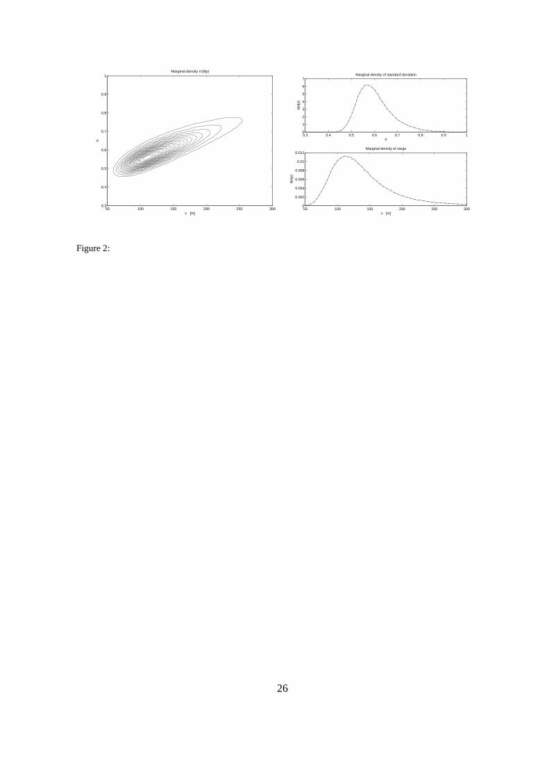
The set of parameter values defined in equation (12) covers σ ∈ {0.3, 1} and ν ∈ {50, 300}

with gridsize L1 = 50 and L2 = 50. The approximate density π(θ|y) obtained by equation (11)

and (12) is shown in Figure 2 (left) along with marginals π(σ|y) and π(ν|y) in Figure 2 (right,

solid curve). Figure 2 (left) seems similar to results obtained earlier by MCMC sampling, see e.g.

Christensen et al. (2006). This is also visible from Figure 2 (right, dashed curves) which displays

estimates of the marginals using MH sampling with joint updating of x and θ, as described in

Section 3.5. Since the solid and dashed curves in Figure 2 (right) are hard to distinguish, the direct

Laplace approximation appears to be very good.

12

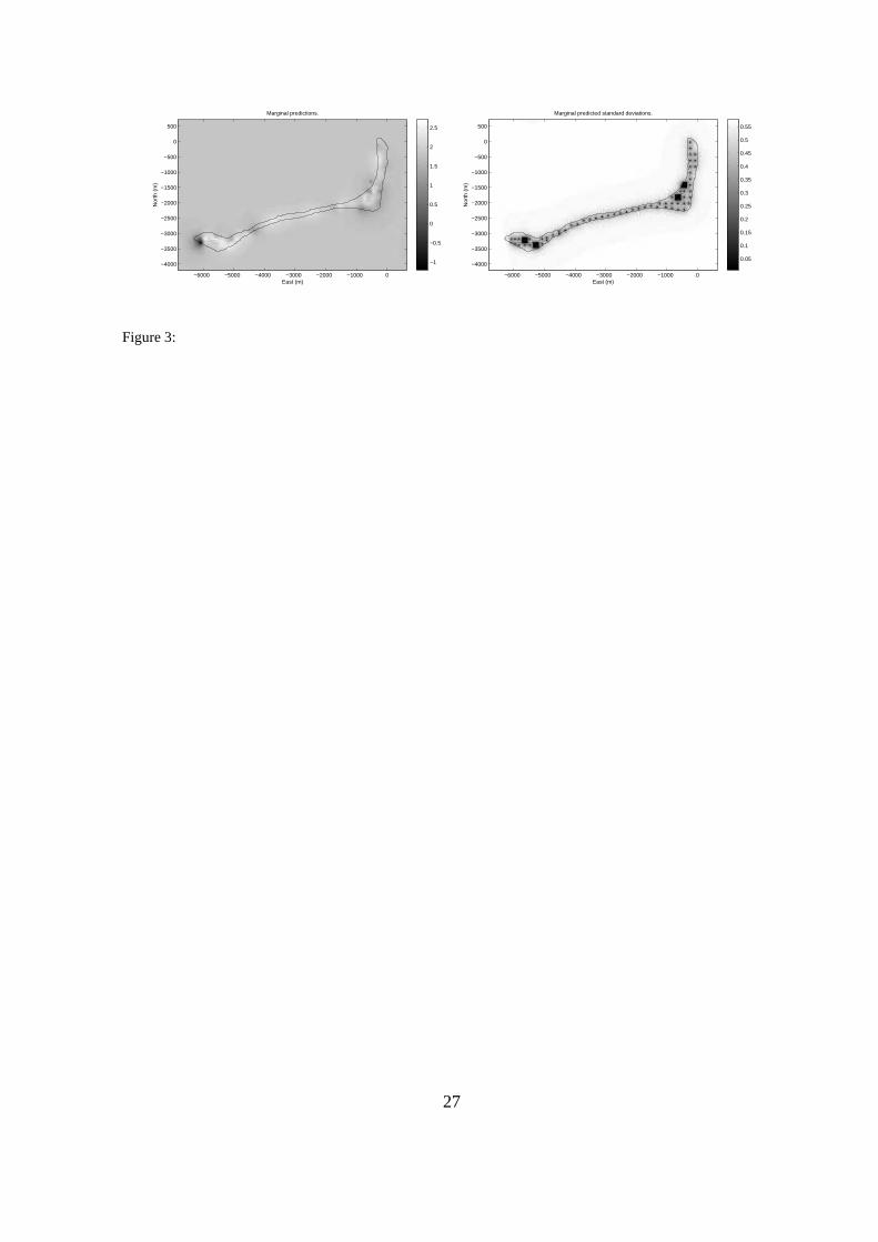
In Figure 3 we show the marginal predictions in equation (15) and standard deviations given by

equation (16). We recognize the measurement locations in the standard deviations and see that the

standard deviations climb to a level of about 0.6 as one goes about 500m away from measurement

locations. Similarly, the spatial predictions in Figure 3 (left) are near the prior mean as we go

away from the island with several measurement locations. The main trends are similar to the ones

obtained by MCMC sampling in Diggle et al. (1998).

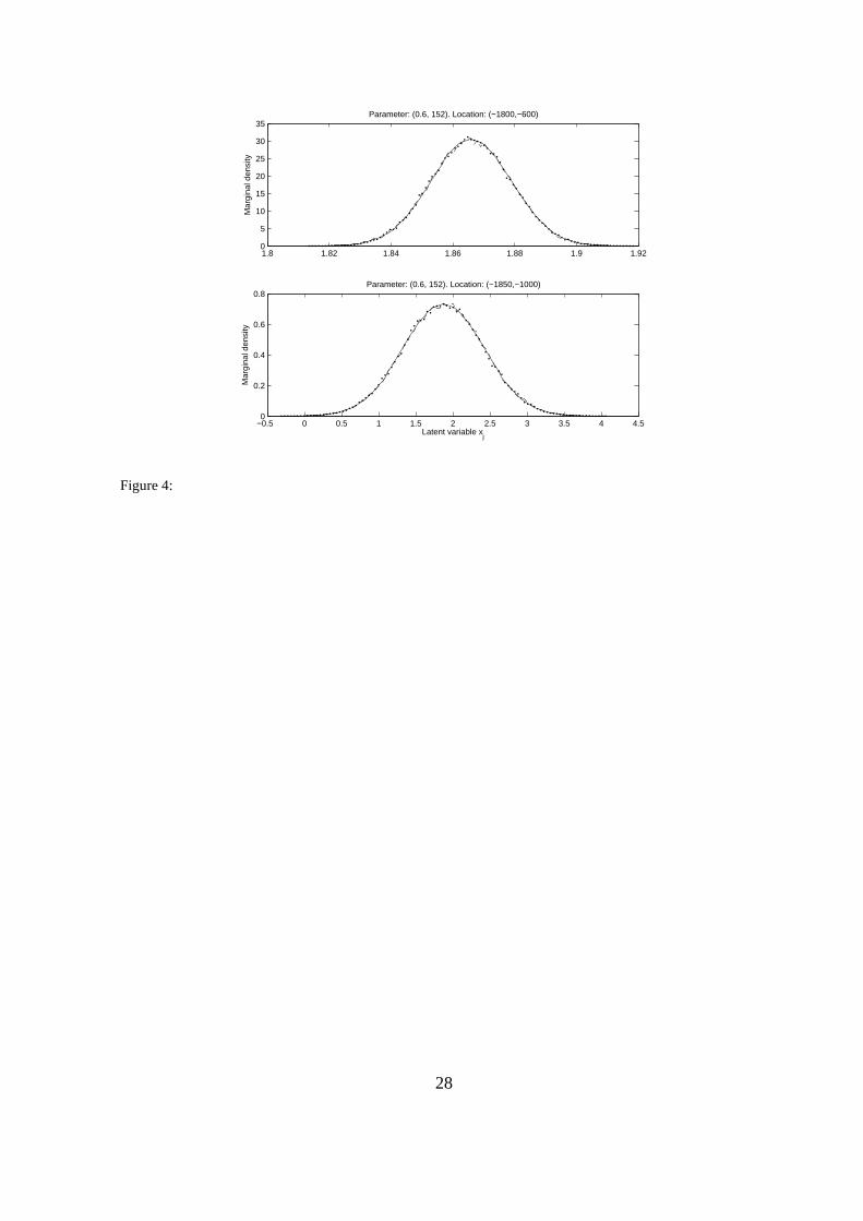
We go on to check the Gaussian approximation that we use for the latent variable via π(x|y, θ).

For this purpose we use Monte Carlo sampling as described in Section 3.5 above. We choose

to evaluate three approximations (direct Gaussian approximation, MH method and importance

sampling) at spatial locations (−1800,−600) and (−1850,−1000). These two are chosen since

they represent locations near and far from registration sites, respectively, see Figure 1. We perform

the testing for parameter θ = (0.6, 152), regarded to be a likely parameter value (Figure 2). In

Figure 4 (solid) we show the approximate densities π(xj|y, θ), where j correponds to the two

spatial locations. Also displayed in Figure 4 (dashed and dotted) are approximations based on

independent proposal MH (dashed) and importance sampling (dotted). The results of the various

approximations displayed in Figure 4 are very similar. Specifically we note that the result of direct

approximate inference is hardly distinguishable from the two Monte Carlo approximations. The

small fluctuations in Figure 4 (solid and dashed) are caused by Monte Carlo error. This error itself

is larger than the differences between the direct approximation and the Monte Carlo estimates.

Figure 2 and 4 show that the results obtained by approximate inference are very similar to

Monte Carlo results, and we note that approximate inference is sufficiently accurate for all practical

purposes in this example. Possible bias effects are so small that it would have no impact on the

decisions made concerning this application. We hence use the term ’practically sufficient’ for our

approximation.

The Monte Carlo algorithms used 100000 proposals. The acceptance probability of the MH

algorithm with joint updating was 0.8, indicating that the approximation is quite good. Importance

sampling resulted in an effective sample size of 90000, indicative of small variability in the weights

for different proposals. For the plotting of Monte Carlo approximations in Figure 4 we split the

13

sample space of xj into 100 disjoint regions in the interval µxj |y,θ ± 4

√

Vxj |y,θ, and thus created

the estimated density curve (dashed and dotted). We avoided smoothing this curve estimate in

order to visualize some of the Monte Carlo error.

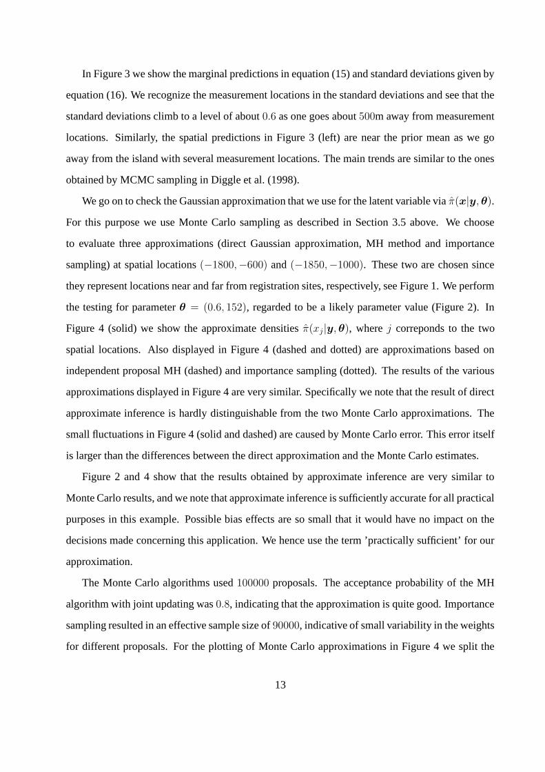
We finally study marginal likelihood values π(y) for various spatial covariance functions. The

choice of covariance model for the latent variable is hence checked. For this purpose we implement

the more general Matern class of covariance functions which is defined by

Σh(σ, ν, κ) = σ2 τκK(τ, κ)

2κ−1Γ(κ), τ = ακδh/ν, h = h2

1 + h22, (19)

where K(·, κ) denotes a modified Bessel function of order κ and Γ(·) is the Gamma function.

In equation (19) the ακ parameter is set so that the correlation is approximately 0.05 at spatial

distance hδ = ν. The Matern family contains the exponential covariance in equation (1) as a

special case when κ = 0.5, while it reduces to the Gaussian (squared exponential) covariance

function when κ = ∞. We calculate the marginal likelihood estimate π(y) in Section 3.3 for four

different Matern covariance models. These models are i) exponential covariance (κ = 0.5), ii)

κ = 1, iii) κ = 2, and iv) Gaussian covariance (κ = ∞). The marginal likelihood is largest for

the exponential covariance in this dataset. The difference in log marginal likelihood is 5.6 when

comparing the exponential with case ii), 9.9 when comparing the exponential with case iii), while

it is 19.6 in favor of the exponential over the Gaussian covariance. Hence, there is evidence of a

steep exponential decline in covariance at zero distance for this dataset.

Our current prototype for direct approximate inference is implemented in Matlab. We are

working on an implementation in C where we avoid using the L1 × L2 grid over parameter space

and use less iterations in the Newton–Raphson search for the conditional mode. The estimated run

time to get the entire inference and prediction solution is then 10-15 seconds.

5. IMPROVED APPROXIMATION FOR π(xj|y, θ)

The direct approximation to the density of xj conditional on data y and fixed hyperparam-

eters θ is π(xj|y, θ) = N(xj; mxj |y,θ, Vxj |y,θ), defined by picking the j-th index of the argu-

ment at the conditional mode mx|y,θ and the j-th diagonal entry of the covariance V x|y,θ =

14

V x|y,θ(mx|y,θ). In this Section we illustrate a method for constructing a more accurate ap-

proximation π(xj|y, θ). The improved version is valuable for two reasons: i) It is more accurate

than the direct approach, and ii) If it is indistinguishable from the direct approximation, the direct

one is checked and confirmed without Monte Carlo sampling. We present the improved version

within the context of our geostatistical special case. A more general description of this approach

is presented in Rue and Martino (2006b).

The improved version is based on

π(xj|y, θ) ∝ π(y|x)π(x|θ)

π(x−j|xj, y, θ), j = 1, . . . , n, (20)

where x−j = (x1, . . . , xj−1, xj+1, . . . , xn)′. For the improved approximation we use a Gaussian

approximation for x−j conditional on xj in the denominator of equation (20). The approximate

marginal, denoted π(xj|y, θ), can be evaluated at a set of xj values and normalized. Note that this

marginal in equation (20) is based on conditioning on xj and using a Laplace approximation to

cancel out the remaining variables x−j . It is hence more accurate than the direct approach which

fits a Gaussian as the joint distribution for all variables. In the choice of evaluation points for xj in

equation (20) we are guided by mxj |y,θ and

√

Vxj |y,θ which are already avaiable from the direct

Gaussian approximation in Section 3.

We fit π(x−j|xj, y, θ) in the denominator of equation (20) by introducing a fictitious measure-

ment xj defined by π(xj|xj) = N(xj ; xj, ζ2), where ζ = 1−6, a very small number. In practice this

means that xj is fixed at the value of the fictitious measurement xj . The denominator in equation

(20) is then interpreted as

π(x−j|xj, y, θ) = π(x|z, θ), z = [z(y, mxs|y,θ), xj]. (21)

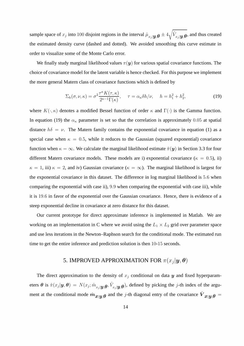
We choose to evaluate equation (20) at the mean of this density given by

µx|y,θ = β + CAR−1

(z − Aβ), R = ACA′+ P , (22)

where the matrices A and P are

A =

A

aj

P =

P 0

0 ζ2

, (23)

15

and aj is a 1 × n vector of zeros except for entry j which equals one. The mean in equation (22)

is computed efficiently in the Fourier domain using that C is block circulant, see Appendix. The

computationally demanding part of the improved approximation is factorizing the term involving

(k + 1) × (k + 1) covariance matrix R.

For the evaluation step we use that

π(x|z, θ) =π(z|x, θ)π(x|θ)

π(z|θ), x = µx|y,θ. (24)

Each term in equation (24) is available, and in particular, π(z|x, θ) = N(z; Ax, P ) and π(z|θ) =

N(z; Aβ, R). The prior for the latent variable, which is also included in the last equation, cancels

when we plug in equation (24) to evaluate π(xj|y, θ) in equation (20).

Recall that the improved approximation π(xj|y, θ) is an additional calculation after the direct

Gaussian approximation has been fitted at the joint mode. The additional calculations are i) finding

the conditional mean for fixed xj , see equation (22), and ii) evaluating the approximate marginal

in equation (20) at this conditional mean. Alternatively, we could evaluate the improved approxi-

mation at the new conditional mode, but using the mean is faster and could be as accurate (Hsiao

et al. 2004).

An improved approximation for the marginal π(xj|y) can be obtained by integrating out the

model parameter θ, like we did in Section 3.4. Our experience is that the difference between direct

and improved approximations is larger for fixed θ.

6. EXAMPLE OF IMPROVED APPROXIMATION

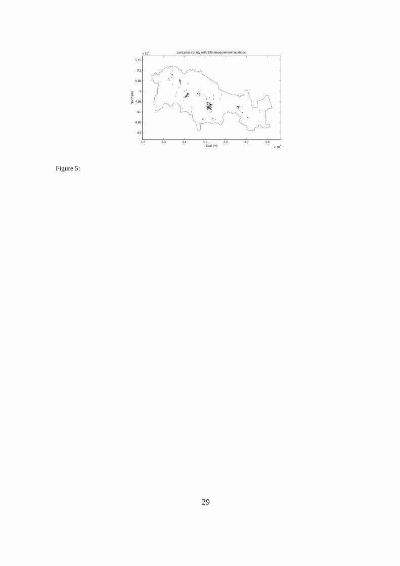
For illustrating the improved approximation we consider the other example in Diggle et al. (1998)

consisting of k = 238 measurements of campylobacter infection in Lancashire district, see Fig-

ure 5. The observations yi = number of campylobacter infection out of enteric infections mi,

i = 1, . . . , k. Each observation is tied to a postal code at a spatial registration site. The infec-

tion data are modeled as a spatial GLMM with a binomial distribution in equation (2). For the

spatial latent variable a grid with interval spacing δ = 30m is constructed. This grid covers the re-

gion from (31970, 47680) to (38660, 51700) in the (North, East) coordinates displayed in Figure 5.

16

Hence, the gridsize is n1 = 135 (North) and n2 = 224 (East), in total n ≈ 30000. Following Rue,

Steinsland and Erland (2004) and Steinsland (2006) an exponential covariance function is used, see

equation (1). We fix the hyperparameter θ = (σ, ν) = (1, 50) in this example. This corresponds to

quite likely parameter values (Steinsland 2006). Again, ten Newton-Raphson iterations are used to

locate the mode of the Gaussian approximation π(x|y, θ)

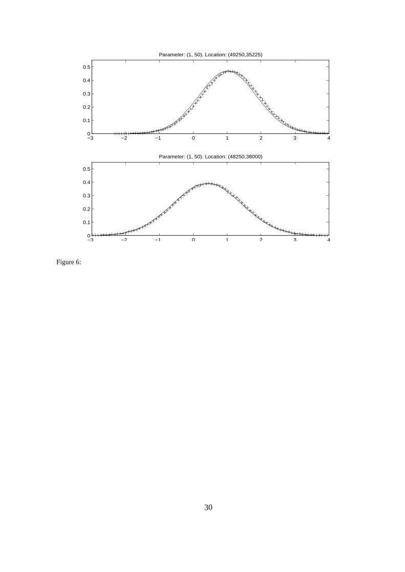
In Figure 6 we show plots of the marginal density for xj at two different spatial locations j. The

two locations are (49250, 35225) and (48250, 38000), representing near and far away from regis-

tration sites, respectively. Figure 6 shows three approximations to the marginal density π(xj|y, θ)

for each of the two locations. The three approximations are as follows: Direct Gaussian approxi-

mation π(xj|y, θ) (solid), improved Gaussian approximation as presented in Section 5 and denoted

π(xj|y, θ) (crossed), and an independent proposal MH approximation obtained by 100000 itera-

tions (dashed) using the joint direct approximation as proposal distribution. In Figure 6 (top),

which displays results of a location only one node (30m) from registration sites, we see that the

direct Gaussian approximation (solid) is slightly biased to the left, while the improved approxi-

mation (crossed) and the MH approximation (dashed) are very similar. In this case the improved

approximation does have an effect on the approximate marginal, possibly since we are near data

nodes and there is much non-Gaussian influence. Hence, the joint Gaussian at the mode does

not capture all features of the marginal density. In Figure 6 (below), which displays results of a

location about 800m from the nearest registration site, the three plots are almost identical. This

indicates that the direct approximation is accurate when there is less non-Gaussian influence.

In this example the direct Gaussian approximation is again ’practically sufficient’, meaning that

for most purposes the slight differences between the solid curve and the others in Figure 6 would

not have any effect. The improved approximation lies on top of the Monte Carlo solution and is

’practically exact’, meaning that the MH sampler cannot detect any possible differences between

the improved approximation and the exact solution which is obtained by MH sampling in the limit.

As pointed out by other authors, see e.g. Diggle et al. (1998) and Steinsland (2006), the data

does not carry much information about the model parameters in this example. We have hence

chosen to treat the hyperparameters as fixed. An interesting line of research is spatial placement of

17

registeration sites for reliable prediction and parameter estimation (Diggle and Lophaven 2006).

7. CONCLUSIONS

In this paper we present fast approximations of marginal posteriors for latent variables and

model parameters for a very common geostatistical model. For this spatial model it has been hard

to design MCMC algorithms that mix adequately. Based on the result of the current paper, we

recommend the approximate solutions which are accurate and fast to compute. They can easily

be part of standard softwares. Fast approximate inference can help to expand the scope of geosta-

tistical modeling. Possible applications of this method include geostatistical design (Diggle and

Lophaven 2006), model choice (Clyde and George 2004) and model assessment (Johnson 2004)

in a geostatistical setting. We have presented the paper in the light of the exponential family like-

lihood model. Other distributions are also possible. The Gaussian approximation for the latent

posterior become worse with extreme likelihoods such as measuring only the absolute value of

the latent variable. Moreover, the measurements do not have to be at a single node, but can be

aggregated at several nodes.

We show results of two methods of approximate inference in the paper. The first method is

’practically sufficient’ in the examples we studied, meaning that for purposes regarding decisions

or model assessment the approximation is accurate enough. The improved version, which provides

a correction to the first approximation, is ’practically exact’ in the examples we studied, meaning

that we only confirmed the approximation when using tedious Markov chain Monte Carlo methods.

In our opinion one would have to run Markov chains for much longer than is typically done to

verify any possible bias of the improved version. However, further research is needed to assess

the quality of each approximation. One might consider computing better, higher order improved

approximations and checking if corrections are still relevant.

We briefly discuss the computational costs and limitations of the direct approximation. Newton-

Raphson optimization to locate the posterior mode requires a matrix inversion of order O(k3) at

each iteration step, finding all conditional variances requires O(nk2), while the fast Fourier trans-

form requires the order of O(n log n). For the case that we consider with n ∼ 10000, k ∼ 100, the

18

variance computation is the most computer intensive part. The limitation of our approach is the

value of k. If k becomes large, say k > 500, the calculations become intractable. The improved

approximation is typically needed only at O(k) cells, i.e. grid nodes near registration sites. The

CPU time of the approximations is in seconds, in constrast to standard Markov chain Monte Carlo

algorithms which typically run overnight.

The special case considered in this paper includes a stationary prior model for the latent vari-

able. This is a very common assumption in geostatistics. Yet, this assumption is easily violated in

two ways; adding a trend in the prior mean or using a covariance matrix that is not block circulant.

One must then include the trend parameters as part of θ and do parametric inference on a larger

sample space. Alternatively one might use a Gaussian Markov random field instead of a Gaussian

random field and include trend parameters as part of the latent variable (Rue and Held 2005).

APPENDIX: COMPUTATIONAL ASPECTS

A.1 Stationary prior distribution:

Let x = (x1, . . . , xn)′ be a Gaussian variable represented on a regular grid of size n = n1n2

with block circulant covariance matrix C. The matrix C might be a function of model pa-

rameters θ but this is suppressed here to simplify notation. We refer to the n1 × n2 matrix

xm = (xm0,0, x

m0,1, . . . , x

mn1−1,n2−1) as the matrix associate of length n vector x. The matrix C

is defined by the covariance between xm0,0 and all other variables as they are positioned on a torus.

We arrange these n covariance entries in an n1×n2 matrix which we denote by cm. We can collect

the n eigenvalues of C in an n1 × n2 matrix λm = dft2(cm) (Gray 2006). Here dft2 denotes the

two dimensional discrete Fourier transform

dft2(cm)j′1,j′

2=

n1−1∑

j1=0

n2−1∑

j2=0

cmj′1,j′

2

exp[−2πι(j1j

′1

n1

+j2j

′2

n2

)], j ′1 = 1, . . . , n1, j′2 = 1, . . . , n2, (25)

with ι =√−1. The determinant of C is the product of all entries in λm. We denote by idft2(dm)

the two dimensional inverse discrete Fourier transform of n1 × n2 matrix dm.

Consider first matrix C multiplied with length n vector v. The n1 × n2 matrix associate of

vector w = Cv can be evaluated by

wm = Re{dft2[dft2(cm) � idft2(vm)]}, (26)

19

where � represents elementwise multiplication. Further, w = Cav is given by

wm = Re{dft2[dft2(cm)?a � idft2(vm)]}, (27)

where (cm)?a means taking every element of cm to the power of a. This last relation is useful for

evaluation and sampling (Rue and Held 2005). For evaluation of the quadratic form we use that

v′C−1v = v′w, where wm is evaluated in equation (27) with a = −1. For sampling we let vm

denote a n1 × n2 matrix of independent variables with mean zero and standard deviation 1, and

with vector associate v. A variable w ∼ N(w; 0, C) can be obtained via its matrix associate using

(27) with a = 1/2 (Chan and Wood 1997).

A.2 Conjugate Gaussian posterior distribution:

Suppose we have prior distribution π(x) = N(x; β, C) and likelihood π(z|x) = N(z; Ax, P ),

z = (z1, . . . , zk)′, where A denotes the sparse k × n matrix of 0s and 1s in equation (3) and as-

sume that n � k. The posterior is π(x|z) = N(x; µx|z; V x|z), where the conditional mean and

covariance are

µx|z = β + CA′R−1(z − Aβ), V x|z = C − CA′R−1AC, R = ACA′ + P . (28)

For evaluation of this posterior we use that

π(x|z) =π(z|x)π(x)

π(z), π(z) = N(z; Aβ, R). (29)

The prior is evaluated using the relationship following equation (27), while the other expressions

only involve k × k matrices and with small k these are fast to evaluate. We can sample from the

posterior as follows: i) Draw a sample from the unconditional density, v ∼ N(v; β, C) using the

relationship following equation (27). ii) Draw a sample w ∼ N(w; z, P ). iii) Set

x = v + CA′R−1(w − Av) = v + u, um = Re{dft2[dft2(cm) � idft2(tm)]}, (30)

where we use equation (26) and tm is the matrix associate of t = A′R−1(w − Av) calculated by

tj =

∑ki′=1 R−1

i,i′(wi′ − vsi′) if si ∈ j

0 else., i = 1, . . . , k, j = 1, . . . , n, (31)

20

using the properties of k × n matrix A. The matrix inversion in equation (31) is for k × k matrix

R and we assume that k is of moderate size.

A.3 Newton-Raphson optimization:

Consider our linearization of the likelihood part in equation (6). For this non-Gaussian case

we find the posterior mode of π(x|y, θ) for fixed θ by iterative linearization using the Newton-

Raphson algorithm. Note first that by setting v = β in step i) and w = z in step ii) of the

sampling step before equation (30), we obtain the posterior mean in step iii) using equation (30).

This is identical to the mean in equation (28). For the approximate Gaussian case we have that

z = z(y, x0s) as in equation (9), using some initial linearization point x0

s. Let next x1s denote

the approximate posterior mean in equation (28) obtained by one application of Newton-Raphson

in equation (30). This process can then be iterated, getting a new transformed measurement z =

z(y, x1s) as in equation (9), then a new posterior mean x2, and so on, until one reach the argument

at the posterior mode denoted by mx|y,θ.

A.4 Evaluation of the Laplace approximation and the acceptance rate:

Let us now bring θ into our notation and study the computational aspects regarding the Laplace

approximation and the acceptance rate of the MH algorithm. We can evaluate the approximate

Gaussian posterior using Bayes formula in a similar manner as in equation (29). This gives

π(x|y, θ) = N(x; mx|y,θ, V x|y,θ) =π(z|x, θ)π(x|θ)

π(z|θ), z = z(y, mxs|y,θ), (32)

where π(z|θ) = N(z; Aβ, R), π(z|x) = N(z; Aβ, P ). The k × k matrices R and P are now

evaluated at the argument at the posterior mode mx|y,θ from the last Newton-Raphson step. For

the Laplace approximation in equation (11) this means that

π(θ|y) ∝ π(y|x)π(x|θ)π(θ)

π(x|y, θ)=

π(y|x)π(θ)π(z|θ)

π(z|x, θ), z = z(y, mxs|y,θ). (33)

The expression only involves k × k matrices and with small k these are fast to evaluate. For the

acceptance rate in equation (18), treating θ as fixed, this means that

min

{

1,[∏k

i=1 π(yi|x′si)]π(x′|θ)

[∏k

i=1 π(yi|xsi)]π(x|θ)

π(x|y, θ)

π(x′|y, θ)

}

= min

{

1,[∏k

i=1 π(yi|x′si)]π(z|x, θ)

[∏k

i=1 π(yi|xsi)]π(z|x′, θ)

}

, (34)

which again only involves k × k matrices and the expression is fast to evaluate.

21

REFERENCES

Ainsworth, L. M., and Dean, C. B., (2006), “Approximate inference for disease mapping”, Com-

putational Statistics & Data Analysis, 50, 2552-2570.

Banerjee, S., Carlin, B. P., and Gelfand, A. E., (2004), “Hierarchical modeling and analysis for

spatial data”, Chapman & Hall.

Breslow, N. E., and Clayton, D. G., (1993), “Approximate inference in generalized linear mixed

models”, Journal of the American Statistical Association, 88, 9-25.

Carlin, B. P., and Louis, T. A., (2000), “Bayes and empirical Bayes methods for data analysis”:

Chapman and Hall.

Chan, G., and Wood, A. T. A., (1997), “An algorithm for simulating stationary Gaussian random

fields”, Applied Statistics, 46, 171-181.

Christensen, O. F., Roberts, G. O., and Skold, M., (2006), “Robust MCMC methods for spatial

GLMM’s”, Journal of Graphical and Computational Statistics, 15, 1-17.

Clyde, M., and George, E. I., (2004), “Model uncertainty”, Statistical Science, 19, 81-94.

Cressie, N. A. C., (1991), “Statistics for spatial data”, Wiley.

Diggle, P. J., Tawn, J. A., and Moyeed, R. A., (1998), “Model-based geostatistics”, Journal of the

Royal Statistical Society, Ser. C, 47, 299-350.

Diggle, P. J., Ribeiro Jr., P. J., and Christensen, O. F., (2003), “An introduction to model-based

geostatistics”, In J. Møller (Ed.) Spatial Statistics and Computational Methods, Lecture notes

in Statistics; 173, 43-86, Berlin: Springer-Verlag.

Diggle, P. J., and Lophaven, S., (2006), “Bayesian Geostatistical Design”, Scandinavian Journal

of Statistics, 33, 53-64.

Gel, Y., Raftery, A. E., and Gneiting, T., (2004), “Calibrated probabilistic mesoscale weather

field forecasting: The geostatistical output perturbation method”, Journal of the American

Statistical Association, 99, 575-583.

Gray, R. M., (2006), “Toeplitz and circulant matrices: A review”, Free book, available from

http://ee.stanford.edu/ ∼gray.

22

Hsiao, C. K., Huang, S. Y., and Chang, C. W., (2004), “Bayesian marginal inference via candidate’s

formula”, Statistics and Computing, 14, 59-66.

Johnson, V. E., (2004), “A Bayesian χ2 test for goodness-of-fit”, The Annals of Statistics, 32,

2361-2384.

McCullagh, P., and Nelder, J. A., (1989), “Generalized linear models”, Chapman & Hall.

Polasky, A., and Solow, A. R., (2001), “The value of information in reserve site selection”, Biodi-

versity and Conservation, 10, 1051-1058.

Press, W. H., Teukolsky, S. A., Vetterling, W. T., and Flannery, B. P., (1996), “Numerical Recipes

in C: The art of Scientific Computing”, Cambridge University Press.

Robert, C. P., and Casella, G., (2004), “Monte Carlo Statistical Methods”, Springer.

Rue, H., Steinsland, I., and Erland, S., (2004), “Approximating hidden Gaussian Markov random

fields”, Journal of the Royal Statistical Society, Ser. B, 66, 877-892.

Rue, H., and Held, L., (2005), “Gaussian Markov random fields, Theory and applications”, Chap-

man & Hall.

Rue, H., and Martino, S., (2006a), “Approximate Bayesian inference for hierarchical Gaussian

Markov random fields”, Journal of Statistical Planning and Inference, To appear.

Rue, H., and Martino, S., (2006b), “Approximate Bayesian inference for latent Gaussian models

using a nested integrated Laplace-approximation”, In Prep.

Shephard, N., and Pitt, M. K., (1997), “Likelihood analysis of non-Gaussian measurement time

series”, Biometrika, 84, 653-667.

Stein, M. L., (1999), “Interpolation of spatial data: Some theory for Kriging”, Springer.

Steinsland, I., (2006), “Parallel exact sampling and evaluation of Gaussian Markov random fields”,

Computational Statistics & Data Analysis, To appear.

Tierney, L., and Kadane, J. B., (1986), “Accurate approximations for posterior moments and

marginal densities”, Journal of the American Statistical Association, 81, 82-86.

23

FIGURE CAPTIONS

Figure 1: Rongelap island with the 157 registration sites for observations of radionuclide concen-

trations.

Figure 2: Rongelap dataset. Left) Direct approximation of joint density of parameters θ = (σ, ν).

Right) Direct approximation of marginal densities for standard deviation σ and spatial correlation

range ν (solid). MH approximation of marginal densities (dashed).

Figure 3: Rongelap dataset. Left) Predicted spatial variable. Right) Marginal standard deviation

of spatial variable.

Figure 4: Rongelap dataset. Conditional density π(xj|y, θ) obtained by approximate inference at

two spatial locations and for parameter values fixed at (σ = 0.6, ν = 152m). Solid is Gaussian

approximation, dashed is approximation obtained by MH sampling, and dotted is approximation

from importance sampling.

Figure 5: Lancashire county with 238 measurement locations of campylobacter infection.

Figure 6: Lancashire dataset. Conditional density π(xj|y, θ) obtained by approximate inference

at two spatial locations and for parameter θ fixed at (σ = 1, ν = 50m). Solid is direct Gaussian ap-

proximation, crossed is improved Gaussian approximation, and dashed is approximation obtained

by MH sampling.

24

FIGURES

−6000 −5000 −4000 −3000 −2000 −1000 0

−4000

−3500

−3000

−2500

−2000

−1500

−1000

−500

0

500

Rongelap Island with 157 measurement locations

East (m)

Nor

th (

m)

Figure 1:

25

ν [m]

σ

Marginal density π (θ|y)

50 100 150 200 250 3000.3

0.4

0.5

0.6

0.7

0.8

0.9

1

0.3 0.4 0.5 0.6 0.7 0.8 0.9 10

1

2

3

4

5

6

7

σ

π(σ|

y)

Marginal density of standard deviation

50 100 150 200 250 3000

0.002

0.004

0.006

0.008

0.01

0.012

ν [m]

π(ν|

y)

Marginal density of range

Figure 2:

26

Marginal predictions.

East (m)

Nor

th (

m)

−6000 −5000 −4000 −3000 −2000 −1000 0

−4000

−3500

−3000

−2500

−2000

−1500

−1000

−500

0

500

−1

−0.5

0

0.5

1

1.5

2

2.5

Marginal predicted standard deviations.

East (m)

Nor

th (

m)

−6000 −5000 −4000 −3000 −2000 −1000 0

−4000

−3500

−3000

−2500

−2000

−1500

−1000

−500

0

500

0.05

0.1

0.15

0.2

0.25

0.3

0.35

0.4

0.45

0.5

0.55

Figure 3:

27

1.8 1.82 1.84 1.86 1.88 1.9 1.920

5

10

15

20

25

30

35Parameter: (0.6, 152). Location: (−1800,−600)

Mar

gina

l den

sity

−0.5 0 0.5 1 1.5 2 2.5 3 3.5 4 4.50

0.2

0.4

0.6

0.8Parameter: (0.6, 152). Location: (−1850,−1000)

Mar

gina

l den

sity

Latent variable xj

Figure 4:

28

3.2 3.3 3.4 3.5 3.6 3.7 3.8

x 104

4.8

4.85

4.9

4.95

5

5.05

5.1

5.15

x 104

East (m)

Nor

th (

m)

Lancaster county with 238 measurement locations.

Figure 5:

29

−3 −2 −1 0 1 2 3 40

0.1

0.2

0.3

0.4

0.5

Parameter: (1, 50). Location: (49250,35225)

−3 −2 −1 0 1 2 3 40

0.1

0.2

0.3

0.4

0.5

Parameter: (1, 50). Location: (48250,38000)

Figure 6:

30