Appropriate Starter for Solving the Kepler's...

International Journal of Computer Applications (0975 – 8887)

Volume 89 – No.7, March 2014

31

Appropriate Starter for Solving the Kepler’s Equation

Reza Esmaelzadeh Space research institute

Tehran, Iran

Hossein Ghadiri Space research institute

Tehran, Iran

ABSTRACT

This article, focuses on the methods that have been used for

solving the Kepler’s equation for thirty years, then Kepler’s

equation will be solved by Newton-Raphson’s method. For

increasing the stability of Newton’s method, various guesses

studied and the best of them introduced base on minimum

number repetition of algorithm. At the end, after studying

various guesses base on time of Implementation, one

appropriate choice first guesses that increase the isotropy and

decrease the time of Implementation of solving is introduced.

Keywords

Kepler’s equation; initial guesses; iterative solution; Newton -

Raphson method

1. INTRODUCTION Various problems are solved by Kepler’s equation. This

equation is used for describing movement of a body under

central gravity. Kepler’s equation looks simple and shows as

below [1]:

𝑀 = 𝐸 − 𝑒𝑠𝑖𝑛𝐸 (1)

𝑒 ∈ [0,1]

𝑀 ∈ [0,2𝜋] Where 𝐸 designates eccentric anomaly, 𝑀 designates mean

anomaly, and 𝑒 designates eccentricity. This equation can be

used to determine the relationship of time and angle place of

the body in the orbit. In some cases, 𝐸 is given and also 𝑒 is

determined and 𝑀 is unknown, in this case, equation (1) can

be directly used. But most of the time, 𝑀 and 𝑒 are determined

and 𝐸 must be calculated. In this case, equation (1) cannot be

directly used.

During years, for solving Kepler’s equation, many methods

are introduced. Colwell [2] provides an in-depth survey of

solution methods. In following of Colwell’s work, a brief

survey of solution methods of Kepler’s Equation that are

published from 1979 until now is explained. Then, choice

Newton’s method for solving Kepler’s equation and scrutiny

convergence and time of Implementation of this method for

several first guesses and choose the best of them. Finally, use

guesses that reduce the time of Implementation of Newton-

Raphson’s method and have desirable convergence rate for

solving equation.

2. METHOD FOR SOLVING KEPLER’S

EQUATION Solving Kepler’s Equation attracts many scholars. Although,

this equation looks sample, cannot be solved analytically and

other methods must to be used. The methods that suggested

for solving Kepler’s equations can be classified in three

categories: classic methods, non-iteration method and

iteration methods.

2.1 Classic Method These methods depend on using power series. 𝐸 power series

is one kind of them that known as Lagrange series [3]:

𝐸 = 𝑀 + 𝑎𝑛𝑒𝑛

∞

𝑛=1

(2)

If 𝑒 is small enough, Lagrange series is convergent and the 𝐸

with a good accuracy will be found. But this series is

divergent for 𝑒 > 0.66 and the more parameters the worse

result, the parameters of Lagrange series must be reduced, too.

Another method is Fourier series that is shown as below [3]:

𝐸 = 𝑀 + 2

𝑛𝐽𝑛 𝑛𝑒 sin(𝑛𝑀)

∞

𝑛=1

(3)

𝑗𝑛 is known as the Bessel function and defined as follows:

𝐽𝑛 𝑥 = (−1)𝑘

𝑘! (𝑛 + 𝑘)!(𝑥

2)𝑛+2𝑘

∞

𝑘=0

(4)

Series solution of Bessel function is convergent for all values

𝑒 < 1. Sentences of series to be increased, more accurate

solutions are closer to Kepler’s equation. Another method is

using Taylor series expansion to approximate the Kepler’s

equation.

𝑓 𝑥 = 𝑓(𝑥)𝑛𝑥𝑛

𝑛!

∞

𝑛=0

(5)

If the series is convergent, approximation of the 𝑓(𝑥) function

will result for small values of 𝑥. Depending on what the

function of 𝑓(𝑥) is considered, different solutions can be

represented. According to what was mentioned, classical

methods of solving Kepler’s equation based on the direct use

of the series expansion. There are other methods, some of

them use series expansion, but as a part of the whole

procedure, these methods are called direct or non-iterative

methods.

2.2 Non-Iterative Methods Such methods are a non-iterative solution of Kepler’s

equation and like the classic methods directly provide

estimate of Kepler’s equation. In 1987, Mikkola [4] presented

a non-iterative two-step solution; initially provided below

approximation by using an auxiliary variable and 𝐴𝑟𝑐𝑠𝑖𝑛𝑒

function expansion.

𝐸 = 𝑀 + 𝑒(3𝑠 − 4𝑠3) (6)

Mikkola’s method is a direct solution of Kepler’s equation

with a desirable precision.

In 1995, Markly [5] published a solution that is based on Pedé

estimating of 𝑠𝑖𝑛𝑒 function. In his method, he tried to

minimize the using of trigonometric function. In 2006,

Feinstein [6] provide a non-iterative solution with using



32

dynamical discretization techniques combined with dynamic

program that was superior of all published methods. In 2007,

Mortari and Clocchiatti [7] provided a non-iterative solution

for Kepler’s equation with the Bézier curves. Compare with

dynamic discretization method, this method does not need any

pre-computed information.

2.3 Iterative Methods Although non-iterative methods for solving Kepler’s equation

worked, a number of researchers have devised iterative

numerical methods that base on Newton-Raphson method.

The idea of Newton-Raphson’s method is to approximate the

nonlinear function 𝑓 𝑥 by the first two terms in a Taylor

series expansion around the point 𝑥. Newton-Raphson’s

method is defined as follows [1]:

𝑓 𝐸 = 𝐸 −𝑀 − 𝑒 𝑠𝑖𝑛𝐸

𝑥𝑛+1 = 𝑥𝑛 −𝑓(𝑥𝑛)

𝑓′(𝑥𝑛)

(7)

For Newton’s method, the rate of convergence is said to be

quadratic that is a very desirable property for an algorithm to

possess. But, if the initial guess is not sufficiently close to the

solution, i.e., within the region of convergence, Newton’s

method may diverge. In fact, Newton’s method behaves well

near the solution (locally) but lacks something permitting it to

converge globally. The second problem occurs when the

derivative of the function is zero. In fact, Newton’s method

loses its quadratic convergence property if the slope is zero at

the solution. Therefore, this method requires that the slop of

the function is computed on each iteration and mustn’t be zero

[8]. Halley generalized the Newton’s method by applying the

second derivative that resulted from Taylor series expansion

[6]:

𝑥𝑛+1 = 𝑥𝑛 −2𝑓(𝑥𝑛)𝑓′(𝑥𝑛)

2[𝑓′ 𝑥𝑛 ]2 − 𝑓(𝑥𝑛)𝑓′′ (𝑥𝑛) (8)

Additional terms of Halley method include additional

calculation on each iteration. His method is more dependent

on the initial guess but have a strong convergence property

[9].

Proper choice of the initial guess can greatly reduce the

computation and guarantee the convergence of method. In

1978, Smith [10] found that the root of Kepler’s equation is

between two values 𝑀 and 𝑀 + 𝑒 by replacement of with 𝐸.

Then, by using the equation of a straight line between 𝑀 and

M+e, introduced this initial guess for Kepler’s equation [10]:

𝐸0 = 𝑀 + 𝑒𝑠𝑖𝑛𝑀

1 − sin 𝑀 + 𝑒 + 𝑠𝑖𝑛𝑀 (9)

In fact, his initial guess is a linear approximation of the root of

Kepler’s equation between two points 𝑀 and 𝑀 + 𝑒. He

compared this initial guess with Newton’s method in two

regions with some other value. Regions deemed by him as

follows:

Region 1: 0.05 ≤ M ≤ π and 0.01 ≤ 𝑒 ≤ 0.99 .

Region 2: 0.005 ≤ 𝑀 ≤ 0.4 and 0.95 ≤ 𝑒 ≤ 0.999 .

His guesses are in the Table 1. Smith’s criterion for a good

initial guess was the average number of iterations to reach a

solution by Newton’s method in each region. He considered

tolerance 5×10-8 to stop the algorithm. Finally, after

comparing the initial guess concluded that without initial

guess 𝑀 + 𝑒, initial guess (9) is the best of the number of

iterations. Difference between the Smith’s initial guess and

𝑀 + 𝑒 in the region 2 is not big. So, the initial guess

introduced as the best one. By using it the Newton’s method

doesn’t need to add correction clauses to avoid divergence

and the number of iteration of this approach is also desirable.

In 1979, Edward NG [9] used a method like Halley. He

considered for distinct areas in space (𝑀, 𝑒), and used a

different value for each area. The first three areas had current

calculations, but found that the Kepler’s equation treats like a

third degree function near this point (𝑀, 𝑒) = (0,1); so, used

third degree root for this area.

Another iterative method was introduced by Danby [11] in

1983, he argued that the degree of convergence goes upper,

the sensitivity of initial value and risk of diverging reduced.

Danby method shows as below:

𝑥𝑛+1 = 𝑥𝑛+𝛿𝑛

𝛿𝑛1 = −𝑓

𝑓′ (10)

𝛿𝑛2 = −𝑓

𝑓′ −12𝛿𝑛1𝑓

′′

(11)

𝛿𝑛3 = −𝑓

𝑓′ −12𝛿𝑛2𝑓

′′ +16𝛿𝑛2

2 𝑓′′′

(12) By using equation (10), the Newton’s method with second

degree convergence will be resulted. If equation (11) used, the

Halley’s method with third degree convergence will be

resulted and using equation (12) will result fourth degree

convergence. Danby used initial guess 𝐸 = 𝑀 in his article,

but later in 1987 [12], understood that division of computing

is useful in two regions. So declared below guesses:

𝐸0 = 𝑀 + 6𝑀

13 −𝑀 𝑒2 0 ≤ 𝑀 < 0.1

𝑀 + 0.85𝑒 0.1 ≤ 𝑀 ≤ 𝜋

(13)

In 1986, Serafin [13] stated that a good choosing for initial

guess 𝐸, needed rang the root of 𝐸 belong to it. He defined

intervals that include root of Kepler’s equation by using the

property of 𝑠𝑖𝑛𝑒 function. Table 2 shows his results. In the

same year, Conway [14] stated a method base on Leguerre’s

method that using for finding the root of a polynomial.

𝑥𝑖+1 = 𝑥𝑖 −𝑛𝑓(𝑥𝑖)

𝑓 ′(𝑥𝑖) ± 𝑛 − 1 2(𝑓′(𝑥𝑖))2 − 𝑛(𝑛 − 1)𝑓 ′′ (𝑥𝑖) (14)

Table 1. Smith’s initial guesses

Initial guesses 𝐸0 = 𝑀

𝐸0 = 𝑀 + 𝑒

𝐸0 = 𝑀 + 𝑒 𝑠𝑖𝑛 𝑀

𝐸0 = 𝑀 + 𝑒𝑠𝑖𝑛𝑀

1 − sin 𝑀 + 𝑒 + 𝑠𝑖𝑛𝑀

𝐸0 = 𝑀 + 𝑒 sin𝑀 + 𝑒2 sin𝑀 cos𝑀

𝐸0 = 𝑀 + 𝛼 1 −𝛼2

2 , 𝛼 =

𝑒 sin𝑀

1 − 𝑒 cos𝑀



33

He selected 𝑛 = 5. The convergence of this method,

regardless of the initial guess is guaranteed. Odell and

Gooding [15], in a part of their article studied twelve different

initial guesses. They believe that rapid convergence in small

𝑀, and big e, only can be possible when initial value shows a

good status of 𝐸. Then, they stated their method. In 1989, Taff

[16] evaluated thirteen different initial guesses and finally the

best and simplest initial guess and solution stated in order

𝐸0 = 𝑀 + 𝑒 and Wegstein’s method. Nijenhuis in 1991 [17] in his article, divided (𝑀, 𝑒) space to four areas and using a different initial guess for each area. His work was like Edward regardless stated different

areas. His initial guesses are:

1- Area of A that includes big M:

𝐸 =𝑀 + 𝑒𝜋

1 + 𝑒 (15)

2- Area of B for middle M:

𝐸 =𝑀

1 − 𝑒 (16)

3- Area of C for small M:

𝐸 =𝑀

1 − 𝑒 (17)

4- Area of D includes a space near the point

(𝑀, 𝑒) = (0,1) that uses Mikkola’s method:

𝐸 = 𝑀 + 𝑒(3𝑠 − 4𝑠3) (18) Outline of his method contain three steps. First, space

of (𝑀, 𝑒) is divided into four separate areas and defines the

initial guess for each area. Second, refine initial guesses of

three areas by one use of Halley’s method and for area of

four, by one use of Newton’s method. Third, modified

Newton’s method used for solving Kepler’s equation. His

modification of Newton’s method is different from what

Danby used. Chobotov [18] compared Newton’s method with

Conway’s method. He shows although convergence of

Conway’s method is guarantee, Newton’s method for

computing the execution time is preferred. In 1997, Vallado

[19] solved the Kepler’s equation for elliptic, parabolic and

hyperbola orbits. For elliptical and hyperbola orbits, studied

the number of iteration of Newton’s method for three below

initial guess:

𝑀 (19) 𝑀 + 𝑒 (20)

𝑀 + 𝑒 𝑠𝑖𝑛𝑀 +𝑒2

2𝑠𝑖𝑛2𝑀

(21)

Table 2. Intervals of 𝑬𝟎

𝑬𝟎 𝑴 ∈

𝑀

1 − 2𝑒𝜋

≤ 𝐸 ≤ 𝑀

1 − 𝑒

[0, 1 − 𝑒𝛼]

𝑀

1 − 2𝑒𝜋

≤ 𝐸 ≤ M + e [1 − 𝑒𝛼0 ,𝜋

2− 𝑒]

𝑀 + 2𝑒

1 + 2𝑒𝜋

≤ 𝐸 ≤ M + e [ 𝜋

2− 𝑒,𝜋 − (1 − 𝑒𝛼0)]

𝑀 + 2𝑒

1 + 2𝑒𝜋

≤ 𝐸 ≤ 𝑀 + 𝑒𝜋

1 + 𝑒

[𝜋 − 1 − 𝑒𝛼0 ,𝜋]

He concluded that Newton’s method with initial guess (21)

compare with two others is convergent with less number of

iteration. But due to transcendental function, amount of

computing time is more than two others. He understood initial

guess (20) is 15% faster than guess (19), while the initial

guess of (21) is only 2% faster. He choose initial guess (20)

for elliptic and hyperbola orbits base on the overall

computation time to avoid the divergence of Newton’s

method and reduce the computation time. In 1998, Charles

[20] stated the Newton’s chaotic behavior and examined it for

these guesses: 𝐸0 = 𝑀, 𝐸0 = 𝜋. He stated that Newton’s

method all the time is convergent for 𝐸0 = 𝜋, but for E0 = M

there is a possibility of divergence. Bellow equation is

provided to obtain a better initial guess:

𝐸0 = 𝑀 + 𝑒[(𝜋2𝑀)1

3 −𝜋

15𝑠𝑖𝑛𝑀 −𝑀] (22)

Curtis, in 2010 [3], used following initial guesses for the

solution of Kepler’s equation:

𝐸0 = 𝑀 +

𝑒

2 , 𝑀 < 𝜋

𝑀 −𝑒

2 , 𝑀 > 𝜋

(23)

Among the presented paper, these that have focused on

iterative methods are considered and after collecting used

initial guesses, examine them with suggested method and

choose the best of them in term of the number of iterations.

Choosing a good initial guess can significantly reduce the

number of required iterations. In general, two clear demand of

an initial guess for solving Kepler’s equation must be fast and

accurate enough. Being a fast initial guess can be determined

by counting the number of iteration do reach a solution or by

measuring time of computation.

Table 3 shows the initial guesses that will be tested. First

guess from Table 3 is the simplest that can be considered. The

root of Kepler’s equation is between two values, these values

as guesses 2 and 3 that belong to Smith’s work are considered.

The conjectures of 4, 5 and 6 from Table 3, are obtained from

𝐸 power series expansion that has one, two and three

sentences. The conjecture of 7 from Table 3 results of this

unequal | sin𝐸| ≤ |𝐸| and 𝑀 −𝐸 = 𝑒 sin𝐸 [13]. Conjectures

of 8 and 9 belong to Smith’s work. Conjecture 11, is resulted

of one using Newton- Raphson’s method on initial 𝜋 value.

Conjectures 12, 20, 21, 22 from Table 3 are the solution of

S9 , S8 , S10، S12 Odell and Gooding.

Conjecture 13 from Table 3 belongs to Danby in 1987. The

conjecture 14 is the result of linear interpolation between 2

and 16 conjectures. Conjecture 16, introduced by Edward Ng.

conjectures 17 and 18 from Table 3 are the above and below

roots of Kepler’s equation that introduce by Serafin, and

conjecture 19 belongs to Charles paper.

3. THE PROPOSED ALGORITHM Two important factors are considered in the compassion of the

iterative methods are: Number of iterations and how much

work must the considered method do for each iteration. The

ideal solution is a balance between these two indicators. Since

Newton’s method known standard method for solving

Kepler’s equation and among the method’s that have been

proposed so far, has the lowest calculations, this method will

be chosen and try to minimize the number of iterations by

selecting a good initial guess. The only problem with this

method is the possibility of divergence in some areas that can

be solved by defining of different initial guesses for some



34

areas first of all. First, rough initial guesses are refined with

one use of Newton’s method.

𝑓 𝐸 = 𝐸 −𝑀 − 𝑒 𝑠𝑖𝑛𝐸

𝐸1 = 𝐸0 −𝑓(𝐸0)

𝑓′(𝐸0) (24)

Then these refined guesses are used as the starter in the

solution of Kepler’s equation. The using algorithm has two

steps: first, using Newton’s method on the initial guesses,

second, solving Kepler’s equation by Newton’s method and

refined guesses. To stop this algorithm, this tolerance (10-10 )

has been considered.

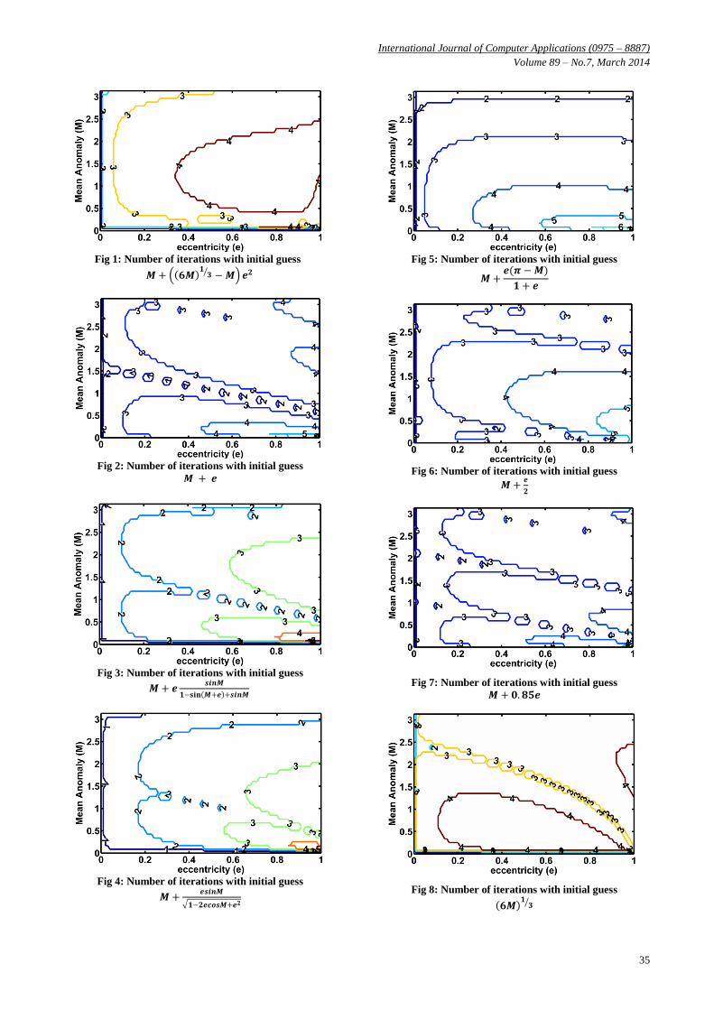
4. RESULTS By using any of the initial guess in Table 3, the Kepler’s

equation is solved in this range 0 ≤ e ≤ 1, 0 ≤ 𝑀 ≤ 𝜋 with

semi-major axis with this length 𝑎 = 5850.6753 𝑘𝑚 by

MATLAB software. Then results introduce in 𝑀 − 𝑒

diagrams. Some of them are showed in below.

In Figure 1, the lowest iteration occurs at small M. Important

property of this is no divergence near the singularity point

(𝑀, 𝑒) = (0,1). The number of iterations of this guess in

small M is less than guesses number 8 and 12 from Table 3. In

Figure 2, almost three repeats for middle 𝑀 is observed.

According to Figures 3 and 4, Newton’s method in a wide

range of space (𝑀, 𝑒) has the lowest iteration but near the

point (𝑀, 𝑒) = (0,1) number of iterations increased. In Figure

5, best performance for M > 2 can be observed. Figure 6

shows the five repeats, but this guess shows increasing the

number of iteration for small 𝑀, e > 0.99 and going to

become divergence. According to the Figure 7, guess number

13 from table 3 has better convergence than initial guess

number 10 from Table 3. According to Figure 8, guess

number 16 from Table 3, has three iterations in wide space

has the best performance in small 𝑀.

Among the initial guesses were examined, two conjectures 8

and 12 from Table 3, have the best performance of number of

iteration in the whole space. On the other hand, these are the

fastest guesses of convergence. So they will be chosen

because they supply an overall convergence for Newton’s

method with minimum number of iteration. For reaching the

minimum iteration in the whole space (𝑀, 𝑒), it is divided

into three area and have been considered an initial guess for

each area according to the results.

𝐸0 =

𝑀 + 6𝑀

13 −𝑀 𝑒2 , 0 ≤ 𝑀 ≤ 0.25

𝑀 + 𝑒𝑠𝑖𝑛𝑀

1 − sin 𝑀 + 𝑒 + 𝑠𝑖𝑛𝑀 , 0.25 ≤ 𝑀 ≤ 2

𝑀 +𝑒𝑠𝑖𝑛𝑀

1 − 2𝑒𝑐𝑜𝑠𝑀 + 𝑒2 , 2 ≤ 𝑀 ≤ 𝜋

(25)

Table 3. Initial guesses

𝑬𝟎 𝑬𝟎

1 𝜋 12 𝑀 +

𝑒𝑠𝑖𝑛𝑀

1 − 2𝑒𝑐𝑜𝑠𝑀 + 𝑒2

2 𝑀 13 𝑀 + 0.85𝑒

3 𝑀 + 𝑒 14 𝑀 + 6𝑀 1

3 −𝑀 𝑒2

4 𝑀 + 𝑒 𝑠𝑖𝑛𝑀 15 𝑀 − 𝑒

5 𝑀 + 𝑒 𝑠𝑖𝑛𝑀 +

𝑒2

2𝑠𝑖𝑛2𝑀

16 6𝑀 1

3

6 𝑀 + 𝑒 𝑠𝑖𝑛𝑀 +

𝑒2

2𝑠𝑖𝑛2𝑀 +

𝑒3

8(3𝑠𝑖𝑛3𝑀

− 𝑠𝑖𝑛𝑀)

17 𝑀 + 2𝑒

1 + 2𝑒𝜋

7 𝑀

1 + 𝑒 18 𝑀 + 𝑒𝜋

1 + 𝑒

8 𝑀 + 𝑒

𝑠𝑖𝑛𝑀

1 − sin 𝑀 + 𝑒 + 𝑠𝑖𝑛𝑀

19 𝑀 + 𝑒[(𝜋2𝑀)1

3 𝜋

15𝑠𝑖𝑛𝑀 −𝑀]

9 𝑀 + 𝛼 −

𝛼2

2 , 𝛼 =

𝑒 𝑠𝑖𝑛𝑀

1 − 𝑒 𝑐𝑜𝑠𝑀

20 𝑠 +𝜋

20𝑒4 𝜋 − 𝑠 , 𝑠 = 𝑀 + 𝑒𝑠𝑖𝑛 + 𝑒2𝑠𝑖𝑛𝑀𝑐𝑜𝑠𝑀

10 𝑀 +𝑒

2 21

𝑠 −𝑞

𝑠 , 𝑠 = [(𝑟2 + 𝑞3)

12 + 𝑟]

13, 𝑞 =

2 1 − 𝑒

𝑒 , 𝑟 =

3𝑀

𝑒

11 𝑀 +

𝑒(𝜋 −𝑀)

1 + 𝑒

22 𝑒𝐸01 + 1 − 𝑒 𝑀, 𝐸01 = 𝜋 −

𝜋 − 1 2(𝜋 − 𝑀)

2 𝜋 −16

2

− (𝜋 − 𝑀)(𝜋 −23

)



35

Fig 1: Number of iterations with initial guess

𝑴 + 𝟔𝑴 𝟏𝟑 −𝑴 𝒆𝟐


𝑴 + 𝒆


𝑴 + 𝒆𝒔𝒊𝒏𝑴

𝟏−𝐬𝐢𝐧 𝑴+𝒆 +𝒔𝒊𝒏𝑴


𝑴 +𝒆𝒔𝒊𝒏𝑴

𝟏−𝟐𝒆𝒄𝒐𝒔𝑴+𝒆𝟐


𝑴 +𝒆(𝝅 −𝑴)

𝟏 + 𝒆


𝑴 +𝒆

𝟐

Fig 7: Number of iterations with initial guess 𝑴 + 𝟎.𝟖𝟓𝒆


𝟔𝑴 𝟏𝟑



36

The minimum number of iteration means that the speed of

convergence is more [13]. Then, rate convergence Newton’s

method increase by these initial values. But, a smaller number

of iterations does not necessarily imply a shorter computation

time. For any given algorithm, the associated computing time

will vary with the computer used to perform the calculation.

The computational efficiency will also depend on the manner

in which the algorithm is implemented. Computation time (or

runtime) reduces whatever number of multiplications,

divisions, square roots, additions, subtractions and

trigonometry function is minor. Then, inexpensive initial

guesses can affect strongly on computation time. Hereinafter,

the runtime of various conjectures will be surveyed briefly

and finally the initial values will be chosen that increase

convergence rate and decrease computation time of Newton-

Raphson’s method at the same time.

Style implementation of Newton-Raphson’s method equal

Tewari’s approach [21]. Used Intel Core i7-2630QM and

DDR III 8G (4GB×2) RAM. The 𝑒 value with step 0.01

between 0 ≤ e ≤ 1 and the 𝑀 value with the time step 60

second (0.875 radiant) are changed that the M’s range is

defined in the range of equation (25) and the run time of

algorithm for each initial guess and range are measured.

According to Figures of 9, 10, 11 the difference between time

of calculating of initial conjectures are low near the 𝜋 point

(millisecond), and also the suggested algorithm for initial

guess 10 from table 3 has the least runtime for 0 < 𝑚 < 0.25

and 0.25 < 𝑚 < 2, in other word, has the maximum speed in

calculations.

Initial guess 11 from Table 3 for 2 < 𝑚 < 𝜋 has the least

runtime. And after it the guess 18 is, but these values are not

as well as values of equation (25) in convergence.

Guess 15 from Table 3 has the lower calculation time in

Comparison of guess 21 from Table 3 for 0 < 𝑚 < 2 it’s because of nonlinear functions in guess 21; so, for having a

good choice of speed of convergence and calculation, the

values of equation (25) are corrected as follow:

𝐸0 =

𝑀 + 𝑒

𝑠𝑖𝑛𝑀

1 − sin 𝑀 + 𝑒 + 𝑠𝑖𝑛𝑀 0 < 𝑀 < 0.25

𝑀 + 𝑒 , 0.25 < 𝑀 < 2

𝑀 +𝑒(𝜋 −𝑀)

1 + 𝑒 , 2 < 𝑀 < 𝜋

(26)

Equation (26) is similar to Odell and Gooding with this

difference that they used 𝑀

1−𝑒 for small 𝑀. The fault of it is, in

the small 𝑀 and 𝑒 near number one become divergent,

because of it, Nijenhuis used Mikkola’s solution for this

range, but increase the time of calculation. In follow,

although, there is no demand for using Mikkola’s solution by

suggested conjectures, the time of calculation will be reduced

and also the speed of convergence will be maintained.

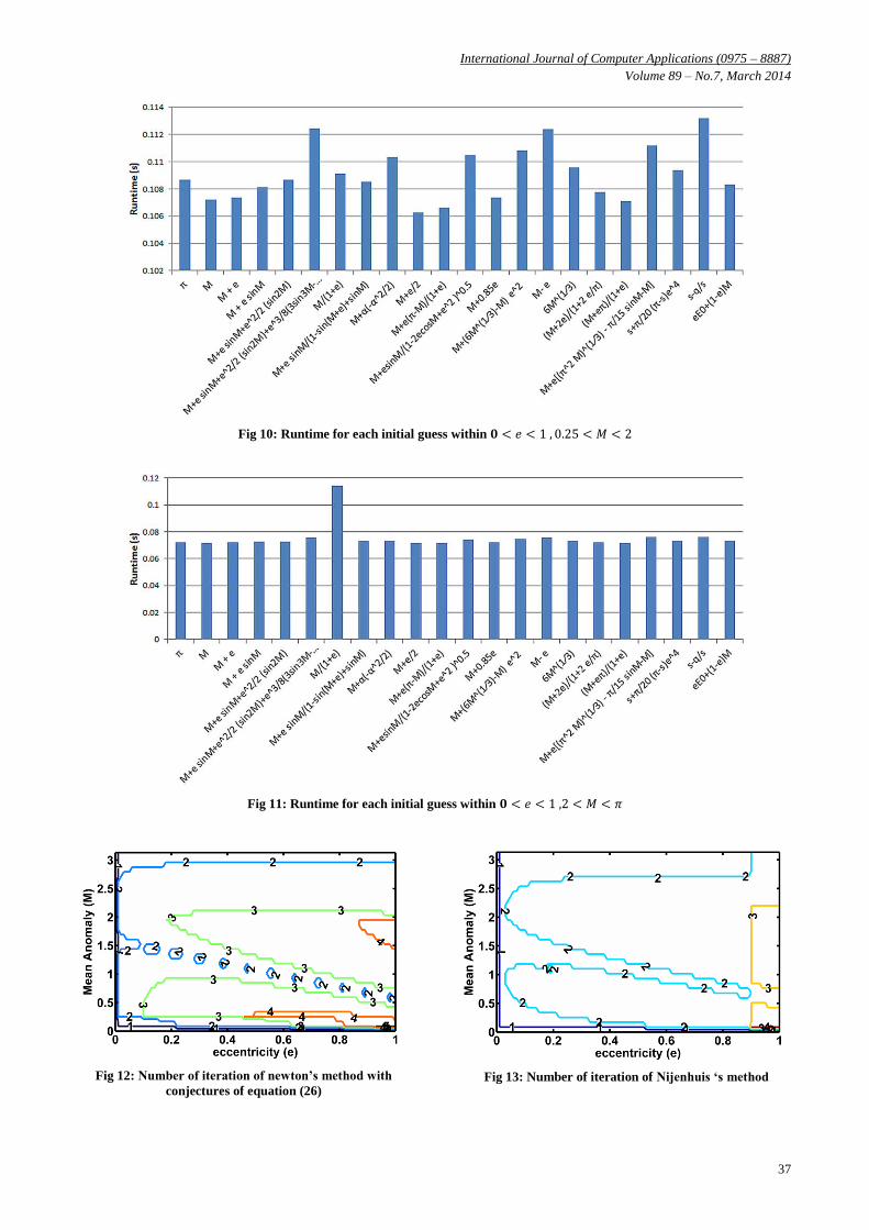
Figures 12 and 13 show Comparison of suggested method

with Nijenhuis method. Nijenhuis’s solution has minimum

repetition because uses Halley’s method for refining the

conjectures and also using Newton’s method of degree of

three for solving Kepler’s equation and reaches to maximum

three repetition in one small area.

However, the suggested method use Newton’s method for

refining conjectures and solving Kepler’s equation has

maximum four repetitions.

Fig 9: Runtime for each initial guess within 𝟎 < 𝑒 < 1, 𝟎 < 𝑀 < 0.25



37

Fig 10: Runtime for each initial guess within 𝟎 < 𝑒 < 1 , 0.25 < 𝑀 < 2

Fig 11: Runtime for each initial guess within 𝟎 < 𝑒 < 1 ,2 < 𝑀 < 𝜋

Fig 12: Number of iteration of newton’s method with

conjectures of equation (26)

Fig 13: Number of iteration of Nijenhuis ‘s method



38

Fig 14: Number of repetition of Nijenhuis‘s method with

conjectures of equation (26)

If suggested conjectures (26) combine with Nijenhuis’s

method, a speed of convergence like Nijenhuis’s solution will

be obtained, and there is no need using Mikkola’s solution for

avoiding divergence. It is showed in Figure 14, also the time

of calculation reduce by deleting Mikkola’s solution.

In the Table 4 the runtime of these three approaches is

compared.

According to Table 4, Newton’s method with the new guesses

has the lowest runtime, and time of calculation of Nijenhuis’s

method with the new guesses reduce almost 4 millisecond, so,

Conjectures of equation (26) are better than others in speed of

convergence and runtime. Combining Conjectures of equation

(26) with better methods (like Nijenhuis’s method) is better

than Newton’s method.

Table 4. comparison of time of whole run

Time of whole run of algorithm

(millisecond)

method

176.791 Equation (26) with

Newton’s method

188.843 Equation (26) with

Nijenhuis’s method

192.681 Nijenhuis’s method

5. CONCLUSION In this article, Newton’s method has been chosen as a known

standard method for solving Kepler’s equation and tested

different initial guesses. The used method has two steps: first,

refining guesses with one use of Newton’s method; second,

solving Kepler’s equation with this method. The speed of

convergence of initial guesses were studied and chosen the

best of them. Then examined the calculation time of them and

to reach these two properties in the whole space (𝑀, 𝑒),

divided this space into three spaces. That used different initial

guesses for each area according to equation (26). The initial

conjectures of equation (26) are not the best but have two

properties in the same time: speed in convergence and

calculation. For this reason, they are considered as optimized

initial conjectures for suggested algorithm. By them, the

solving method reached a good speed in convergence and

time of calculation.

6. REFERENCES [1] R. H. Battin. 2001. An Introduction to the Mathematics

and Methods of Astrodynamics. Revised Edition, AIAA

education series, pp. 160.

[2] P. Colwell. 1993. Solving Kepler equation over three

centuries. Willmann-Bell, Ins.

[3] H. D. Curtis. 2010. Orbital Mechanics for engineering

students. 2nded, Elsevier Aerospace Engineering Series p

163, pp. 168-170.

[4] Mikkola. 1987. A cubic approximation for Kepler’s

equation. Celestial Mech 40. pp. 329-334.

[5] Markley. 1995. Kepler equation solver. Celestial Mech

Dyn Astr 63. pp. 101-111.

[6] S. A. Feinstein, C. A. McLaughlin. 2006. Dynamic

discretization method for solving Kepler’s equation.

Celestial Mech Dyn Astr 96. pp. 49-62.

[7] D. Mortari, A. Clocchiatti. 2007. Solving Kepler’s

equation using Bezier curves. Celestial Mech Dyn Astr

99. pp. 45-57.

[8] J. T. Betts. 2010. Practical Methods for Optimal Control

and Estimation Using Nonlinear Programming. Second

Edition, Siam, Philadelphia. pp. 3.

[9] Edward W .NG. 1979. A general algorithm for the

solution of Kepler’s equation for elliptic orbits. Celestial

Mech 20. pp. 243-249.

[10] Smith. 1979. A simple efficient staring value for the

iterative solution of Kepler’s equation. Celestial Mech

19. pp. 163-166.

[11] J.M.A. Danby, T. M. Burkardt .T.M. 1983. The solution

of Kepler’s equation, I. Celestial Mech 31. pp. 95-107.

[12] J.M.A. Danby. 1987. The solution of Kepler’s equation,

III. Celestial Mech 40. pp. 303-312.

[13] R.A. Serafin. 1986. Bounds on the solution to Kepler’s

equation. Celestial Mech 38. pp. 111-121.

[14] B. A. Conway. 1986. An improved algorithm due to

laguerre for the solution of Kepler’s equation. Celestial

Mech 39. pp. 199-211.

[15] A. W. Odell, R. H. Gooding. 1986. Procedures for

solving Kepler’s equation. Celestial Mech 38. pp. 307-

344.

[16] L. G. Taff, T. A. Brenan. 1989. On solving Kepler’s

equation. Celestial Mech Dyn Astr 46. pp. 163-176.

[17] Nijenhuis. 1991. Solving Kepler’s equation with high

efficiency and accuracy. Celestial Mech Dyn Astr 51. pp.

319-330.

[18] Chobotov. 1996. Orbital Mechanics. 2nded, AIAA

education series.

[19] D. A. Vallado. 2001. Fundamentals of Astrodynamics

and Application. Space Technology Series, McGraw-

Hill. pp. 211, pp. 230-244.

[20] E. D. Charles, J. B. Tatum. 1998. The convergence of

Newton-Raphson iteration with Kepler’s equation.

Celestial Mech Dyn Astr 69. pp. 357-372.

[21] A. Tewari. 2006. Atmospheric and space flight

dynamics. Birkhauser. pp. 105.

IJCATM : www.ijcaonline.org

Appropriate Starter for Solving the Kepler's...

Documents

Transcript of Appropriate Starter for Solving the Kepler's...