Journal of Modern Applied StatisticalMethods

Volume 14 | Issue 2 Article 17

11-1-2015

Approaches for Detection of Unstable Processes: AComparative StudyYerriswamy WooluruJ S S Academy of Technical Education, Bangalore, India, ysprabhu@gmail.com

D. R. SwamyJ S S Academy of Technical Education, Bangalore, India

P. NageshJSS Centre for Management Studies, Mysore, Indi

Follow this and additional works at: http://digitalcommons.wayne.edu/jmasm

Part of the Applied Statistics Commons, Social and Behavioral Sciences Commons, and theStatistical Theory Commons

This Regular Article is brought to you for free and open access by the Open Access Journals at DigitalCommons@WayneState. It has been accepted forinclusion in Journal of Modern Applied Statistical Methods by an authorized editor of DigitalCommons@WayneState.

Recommended CitationWooluru, Yerriswamy; Swamy, D. R.; and Nagesh, P. (2015) "Approaches for Detection of Unstable Processes: A Comparative Study,"Journal of Modern Applied Statistical Methods: Vol. 14 : Iss. 2 , Article 17.DOI: 10.22237/jmasm/1446351360Available at: http://digitalcommons.wayne.edu/jmasm/vol14/iss2/17

Approaches for Detection of Unstable Processes: A Comparative Study

Cover Page FootnoteThis work is supported by JSSMVP Mysore. I, sincerely thank to my Guide Dr.Swamy D.R, Professor andHead of the Department, Industrial Engineering &Management, JSSATE Bangalore and Co-Guide DrP.Nagesh, Professor, Department of Management studies, SJCE, Mysore.

This regular article is available in Journal of Modern Applied Statistical Methods: http://digitalcommons.wayne.edu/jmasm/vol14/iss2/17

Journal of Modern Applied Statistical Methods

November 2015, Vol. 14 No. 2, 219-235.

Copyright © 2015 JMASM, Inc.

ISSN 1538 − 9472

Yerriswamy Wooluru is an Associate Professor. Email him at: jssateb.ac.in.

219

Approaches for Detection of Unstable Processes: A Comparative Study

Yerriswamy Wooluru JSS Academy of Tech. Ed.

Bangalore, India

Dr. D. R. Swamy JSS Academy of Tech. Ed.

Bangalore, India

Dr. P. Nagesh JSS Centre for Mgmt. Stud.

Mysore, India

A process is stable only when parameters of the distribution of a process or product characteristic remain same over time. Only a stable process has the ability to perform in a predictable manner over time. Statistical analysis of process data usually assume that data are obtained from stable process. In the absence of control charts, the hypothesis of process stability is usually assessed by visual examination of the pattern in the run chart. In this paper appropriate statistical approaches have been adopted to detect instability in the process and compared their performance with the run chart of considerably shorter length for assessing its patterns and ensuring the process stability.

Keywords: Process stability, run chart patterns, run test, unstable process

Introduction

The run chart is a most effective and widely used tool for monitoring the stability

of a process by displaying the data to make process performance visible. As long

as the series of points in time exhibit a random pattern, the process is assumed to

have constant mean and standard deviation and no autocorrelation (i.e. stable).

While run charts focus more on time pattern, a control chart focuses on acceptable

limits of the process data. However, in many industrial situations, it becomes

necessary to estimate process parameter whose stability cannot be monitored

using control charts due to lack of data and time for establishing control limits. In

the absence of properly established control charts, process stability can be

evaluated with the help of run chart trend and its pattern, which can be detected

by applying run rules and to conclude the assignable causes present in the process.

In run chart, each observation of a sample have a time variable representing

the time of each data point is measured when data have time related behavior, run

charts are familiar tools to visualize the process behavior. Also Deming (1986)

pointed that when processes ought to behave randomly overtime, run charts can

APPROACHES FOR DETECTION OF UNSTABLE PROCESSES

220

help to identify nonrandom behavior, which can unearth potential for

improvement. Run charts can be used as one of the important tools for diagnosing

and solving various industrial problems, nonrandom patterns are indicative of

process instability. Depending on the causes of process instability the non-random

patterns can be of different types. The SQC Handbook of Western Electric

illustrated various types of unnatural or nonrandom patterns that may occur in the

run chart (Western Electric, 1956). Among these, six types of non-random

patterns of individual observations are upward shift, downward shift, increasing

trend, decreasing trend, cyclic and systematic patterns.

Various statistical tools, such as Regression analysis, ANOVA method, SR

test, INSR test, and Levene’s test have been used to assess the process location

and variation to detect statistical stability of the forging process. These tools have

also been compared with run chart of considerably shorter length to assess the

efficiency of the above statistical methods, and indicate the process stability.

Methodology

The methodology involves the following steps:

1. Understanding the basic concepts and tools to detect process stability

of a manufacturing process.

2. Process data collection.

3. Approaches used for assessing the statistical stability of the process

are

a. Regression Analysis,

b. SR method,

c. INSR method,

d. Run test

e. ANOVA method

f. Levene’s test

4. Construction of Run chart using statistical software MINITAB

5. Compare the performance of the above approaches with Run chart.

6. Conclusion about the performance of the above methods.

WOOLURU ET AL.

221

Data collection and analysis

The data set pertaining to the critical quality characteristic i.e. inner diameter of

piston rings for an automotive engine produced by forging process. The details of

the operation and product specification are presented in Table 1. The required

quality characteristic of 32 consecutive units are measured and presented in Table

2. The basic sample statistics are calculated and presented in Table 3. Table 1. Product description

Part Name Material Operation Specifications Measuring Device

Piston ring Cast steel Forging 74.00 ± 0.05 Dial Gauge

*All dimensions are in mm.

Table 2. Measurements of Piston ring hole diameter in mm.

Sl. no. Hole dia Sl. no. Hole dia Sl. no. Hole dia Sl. no. Hole dia

1 74.030 9 74.011 17 73.996 25 74.014

2 74.002 10 74.004 18 73.993 26 74.009

3 74.019 11 73.988 19 74.015 27 73.994

4 73.992 12 74.024 20 74.009 28 73.997

5 74.008 13 74.021 21 73.992 29 73.985

6 73.995 14 74.005 22 74.007 30 73.993

7 73.992 15 74.002 23 74.015 31 73.998

8 74.001 16 74.002 24 73.989 32 73.990

Table 3. Summary Statistics of the case study data.

Sample size Mean Median Minimum Maximum Range Std. Deviation

32 74.003 74.002 73.985 74.03 0.045 0.0115

Statistical Approaches to Detect Instability

Regression analysis

One way to quantify the change in location is to fit a straight line to the data using

an index variable as the independent in the regression. In this case, the observed

APPROACHES FOR DETECTION OF UNSTABLE PROCESSES

222

values are in the sequential run order and they are collected at equally spaced time

intervals. In this study, index variable are X = 1, 2, 3,… N where N is the number

of observations. If there is no significant drift in the location over time, the slope

parameter would be zero. The scatter diagram of the data reveals a negative linear

association. Therefore, it can be proceeded to find the equation of the regression

line using MINITAB statistical software.

Figure 1. Output of regression analysis table for case study data.

The regression equation is Dia. of Hole = 74.0 - 0.000421 × (X)

Analysis of Variance

Source DF SS MS F P Regression 1 0.0004831 0.0004831 4.03 0.054

Residual Error 30 0.0035964 0.0001199 Total 31 0.0040795

In the output of the regression analysis table for the case study data, the

F-statistic is 4.03. The table value is 4.17 for F (0.05, 1, 30). Since Fcalculated is less

than Ftable value, and the p-value is greater than 0.05. It may be concluded that

there is evidence that slope is almost equal to zero and ensure the process is stable

over time.

x

Dia

of H

ole

35302520151050

74.03

74.02

74.01

74.00

73.99

73.98

S 0.0109490

R-Sq 11.8%

R-Sq(adj) 8.9%

Fitted Line PlotDia of Hole = 74.01 - 0.000421 x

WOOLURU ET AL.

223

SR method (standard deviation ratio method)

The SR test is derived from the square of the ratio of the standard deviation

estimated using all the observations and the standard deviation estimated using

sub group ranges/standard deviations/individual moving ranges. The basis of the

SR test is that if the process is stable, all the approaches would yield similar

estimates for the process standard deviation. In this case statistic, SR is computed

as the ratio of the estimate of the long term variance and the estimate of the short

term variance. The estimated sample variance based on the N observations will

indicate the long term variance and the estimated variance based on the moving

range (MR) method will reveal the short term variance.

Thus,

2

1

1

1

1.128

N

i

y yN

SRMR

(1)

1

N

i

i

y Y N

(2)

1

1

1

1N

i i

i

MR y y N

(3)

Ramirez and Runger (2006) assumed that an approximate F-distribution for

SR, where the effective degree of freedom associated with the numerator and

denominator are considered as (N-1) and 0.62 × (N-1) respectively and

accordingly, it is recommended as an approximate F-test for SR.

APPROACHES FOR DETECTION OF UNSTABLE PROCESSES

224

Table 4. Calculation of Moving Range for the case study data.

Sl. no. Hole dia (yi ) 1i iMR y y Sl. no. Hole dia (yi) 1i iMR y y

1 74.030 - 17 73.996 0.006

2 74.002 0.028 18 73.993 0.003

3 74.019 0.017 19 74.015 0.022

4 73.992 0.027 20 74.009 0.006

5 74.008 0.016 21 73.992 0.017

6 73.995 0.013 22 74.007 0.015

7 73.992 0.003 23 74.015 0.008

8 74.001 0.009 24 73.989 0.016

9 74.011 0.010 25 74.014 0.025

10 74.004 0.007 26 74.009 0.005

11 73.988 0.016 27 73.994 0.015

12 74.024 0.036 28 73.997 0.003

13 74.021 0.003 29 73.985 0.007

14 74.005 0.016 30 73.993 0.008

15 74.002 0.003 31 73.998 0.005

16 74.002 0.000 32 73.990 0.008

2

2368.0974.0029,

32

0.3730.0120,

31

y

MR

MR

d

(4)

d2 = 1.128, Statistical constant for n = 2 (Montgomery, 2009, p.702)

0.012

0.01061.128

.

1 0.373

0.05,31,19.22 1.93

i iy y

F F tab

WOOLURU ET AL.

225

Because SR = 0.012, i.e., (F calculated), F (calculated) < F (table). Hence, it is

concluded that the process is said to be stable.

Instability ratio test (INSR)

The instability ratio is defined as the ratio of the number of data points that have

one or more violation of the Western Electric (1956) rules to the total number of

data points plotted in the process behavior chart for the time period under

assessment. The motivation for the INSR test is that if the process is stable, then it

operates with common cause variation only and over time the observations move

randomly about the central line and typically remain within the upper and lower

control limits. The pattern exhibited in the run chart is called a random pattern.

Appearance of a nonrandom pattern, which can be detected by applying run

rules, is indicative that there is either an assignable cause present in the process or

the process output’s variation has increased. Ramirez and Runger (2006)

considered that the four most popular Western Electric (1956) rules for

application of INSR method. Rules are as follows:

1 point out side of 3σ limits,

8 points in a row on one side of the central line,

2 of 3 points 2σ and beyond on the same side of the central line,

4 of 5 points 1σ and beyond on the same side of the central line.

Then the test statistic, INSR, is noted as follows

Total number of violations with respect to the four rules in the chart

100Total number of observations plotted in the chart

INSR (5)

APPROACHES FOR DETECTION OF UNSTABLE PROCESSES

226

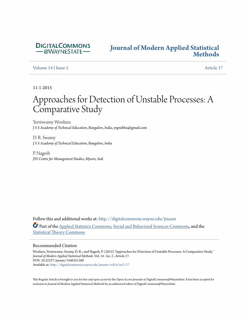
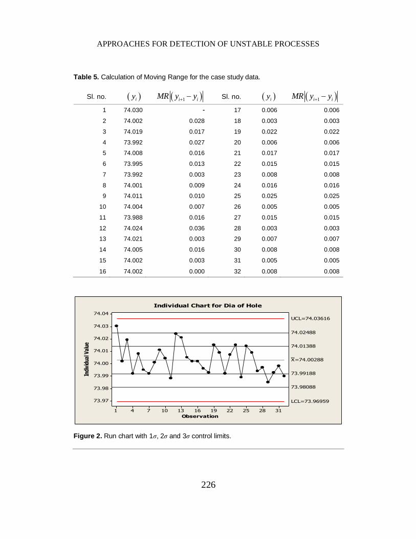
Table 5. Calculation of Moving Range for the case study data.

Sl. no. iy 1i iMR y y Sl. no. iy 1i iMR y y

1 74.030 - 17 0.006 0.006

2 74.002 0.028 18 0.003 0.003

3 74.019 0.017 19 0.022 0.022

4 73.992 0.027 20 0.006 0.006

5 74.008 0.016 21 0.017 0.017

6 73.995 0.013 22 0.015 0.015

7 73.992 0.003 23 0.008 0.008

8 74.001 0.009 24 0.016 0.016

9 74.011 0.010 25 0.025 0.025

10 74.004 0.007 26 0.005 0.005

11 73.988 0.016 27 0.015 0.015

12 74.024 0.036 28 0.003 0.003

13 74.021 0.003 29 0.007 0.007

14 74.005 0.016 30 0.008 0.008

15 74.002 0.003 31 0.005 0.005

16 74.002 0.000 32 0.008 0.008

Figure 2. Run chart with 1σ, 2σ and 3σ control limits.

Observation

Indi

vidu

al V

alue

3128252219161310741

74.04

74.03

74.02

74.01

74.00

73.99

73.98

73.97

_X=74.00288

UCL=74.03616

LCL=73.96959

73.98088

73.99188

74.01388

74.02488

Individual Chart for Dia of Hole

WOOLURU ET AL.

227

Process mean (µ) that represents the central line and the standard deviation

(σ) that determines the distances of the control limits from the central line are

usually unknown, and so these may be estimated from the N observations. The

process means (µ) and standard deviation (σ) are estimated using arithmetic mean

and moving ranges respectively.

Interpretation

a) 1 point out side of 3σ limits, (in Figure 2 no points violate this rule).

b) 8 points in a row on one side of the central line, (in Figure 2 no

points violate this rule).

c) 2 of 3 points 2σ and beyond on the same side of the central line, (in

Figure 2 no points violate this rule).

d) 4 of 5 points 1σ and beyond on the same side of the central line, (in

Figure 2 no points violate this rule).

e) As no points violating the above 4 rules, INSR = 0.00, cutoff value

for Run chart length (N = 32) is 3.125% [8], so the process is said to

be stable.

Variation

To detect a change in variation in the process, Levene’s test has been used it is

based on the median rather than the mean. It assesses the assumptions that

variance of the population from which different samples are drawn are equal. It

tests the null hypothesis that the population variances are equal. If the resulting

p-value of Levene’s test is less than critical value (0.05), the obtained differences

in the sample variances are unlikely to have occurred based on random sampling

from a population with equal variances thus the null hypothesis of equal variances

is rejected and it is concluded that there is a difference between the variances in

the population. It also tests whether two sub samples in a given population have

equal or different variances based on p-values.

Hypothesis Testing: Null hypothesis H0 ; σ1 = σ2 = σ3 = σ4 (There is no

change in variance)

Alternate hypothesis, H0 ; σ1 ≠ σ2 ≠ σ3 ≠ σ4 (There is change in variance)

Levine’s Test has been carried out using the MINITAB software. Since the

p-value is greater than 0.05, the null hypothesis is accepted and hence that there is

no change in variance among the 4 sets in the sample data of 32 consecutive units.

APPROACHES FOR DETECTION OF UNSTABLE PROCESSES

228

ANOVA

This approach is to compare within subgroup variation to between subgroup

variation to detect a difference in subgroup means and aimed at detecting changes

in the process mean only. In this case study, N=32 individual observations are

collected and the ANOVA method is applied by forming subgroups of size 2

using consecutive observations, i.e. there will be N/2 subgroups. Then the test

statistic F is computed as the ratio of the mean sum of squares of subgroups (MS

subgroup) and the mean sum of squares of errors (MS error). Table 6. Analysis of Variance

Sl. no. 1

x 2

x i

x x 2

ix x

2

ji ix x

2

jix x

1 74.030 74.002 74.016 73.996 0.0004 0.000392 0.001192

2 74.019 73.992 74.0055 73.996 9.03E-05 0.000365 0.000545

3 74.008 73.995 74.0015 73.996 3.02E-05 8.45E-05 0.000145

4 73.992 74.001 73.9965 73.996 3.00E-07 4.05E-05 0.000041

5 74.011 74.004 74.0075 73.996 0.000132 2.45E-05 0.000289

6 73.988 74.024 74.006 73.996 0.0001 0.000648 0.000848

7 74.021 74.005 74.013 73.996 0.000289 0.000128 0.000706

8 74.002 74.002 74.002 73.996 0.000036 0.000000 0.000072

9 73.996 73.993 73.9945 73.996 2.30E-06 4.50E-06 0.000009

10 74.015 74.009 74.012 73.996 0.000256 0.000018 0.00053

11 73.992 74.007 73.9995 73.996 1.23E-05 0.000113 0.000137

12 74.015 73.989 74.002 73.996 0.000036 0.000338 0.00041

13 74.014 74.009 74.0115 73.996 0.00024 1.25E-05 0.000493

14 73.994 73.997 73.9955 73.996 3.00E-07 4.50E-06 0.000005

15 73.985 73.993 73.989 73.996 0.000049 0.000032 0.00013

16 73.901 73.87 73.8855 73.996 0.01221 0.000481 0.024901

Table 7. Resulted values from the ANOVA Analysis.

SSFactor = 0.0277684 MSFactor = 0.001

SSE = 0.0026845 MSE = 0.002

SST = 0.03045 Fo = 0.98

WOOLURU ET AL.

229

From Ftable, Fcritical = 2.39 and Fcalculated = 0.98. Since Fcal. < F0.05,15,16, the

process position in time relating to a hole diameter data is not subjected to

significant changes.

Run test for randomness in the sequence.

It tests the runs up and down or the runs above and below the mean by comparing

the actual values to expect values. The statistic for comparison is the chi-square

test [6]. All observations in the sample larger than the median value are given a

positive sign and those below the median are given negative sign. A succession of

values with the same sign is called a run and the number of runs ‘a’ in the

sequence of data points is found and it from the test statistic. For n > 30, this test

statistic can be compared with a normal distribution with mean and the variance,

the test is two-tailed. Data: Sample size: 32 observations, Median: 74.002 Table 8. Values above and below the median.

74.030 74.002 74.019 73.992 74.008 73.995 73.992 74.001 - + - + - - + +

74.011 74.004 73.988 74.024 74.021 74.005 74.002 74.002 - + + - - - - -

73.996 73.993 74.015 74.009 73.992 74.007 74.015 73.989 - + - - + + - +

74.014 74.009 73.994 73.997 73.985 73.993 73.998 73.990 - - + - + + + -

H0: The sequence is produced in a random manner.

H1: The sequence is not produced in a random manner.

Number of observations, N = 32, Number of runs, a = 18

2 1

3a

N

(6)

2 16 29

90a

N

(7)

APPROACHES FOR DETECTION OF UNSTABLE PROCESSES

230

2

2 32 121

3

16 32 295.37

90

a

a

For N > 20, the distribution of ‘a’ (number of runs) is reasonably

approximated by a normal distribution, 2,a aN . This approximation can be

used to test the independence of the observations. In this case the standardized

normal test statistic is developed by subtracting the mean from the observed

number of runs ‘a’ and dividing by the standard deviation.

The test statistic is as follows.

0

a

a

aZ

(8)

0

18 211.30

2.32Z

Test statistic: Z0 = -1.30, Significance level: α = 0.05

Critical value: Z1-α/2 = 1.96, Reject H0, if |Z| > 1.96.

In this case, the test statistic (-1.30) is inside the critical region, the null

hypothesis cannot be rejected and hence it is concluded that the data is random.

The critical value Z0.025 = 1.96. Because |Z0| < Z0.025, the independence

(randomness) of the sequence of the observations cannot be rejected.

Run chart analysis

A run chart is a line graph of data plotted over time. By collecting and charting

data over time, trends or patterns in the process can be revealed. As run charts do

not use control limits, they cannot exhibit if a process is stable. However, they can

show that how the process is running. The run chart can be a valuable tool at the

beginning of a manufacturing process, as it reveals important information about a

process before collecting the enough data to create reliable control limits. Figure 3

shows the Run chart for the case study data constructed using statistical software

MINITAB to assess the stability of the process.

WOOLURU ET AL.

231

Figure 3. Construction of run chart using MINITAB-Statistical software.

The two tests (actual number of runs about median and number of runs up

and down) have been conducted to check the randomness. In both the tests i.e.,

actual number of runs about median and number of runs up and down are close to

the expected number of runs. It implies that the data come from random

distribution. Clusters are groups of points in one area of the charts, cluster

indicate variation due to special causes such as measurement problem. In this case,

approximate p-value is 0.39205, it is greater than 0.05, hence it may be concluded

that there is no clustering in the data. Process stability can be assured by

observing the oscillation of data above and below the center line rapidly. In this

case, Approximate p-value is 0.80602, it is greater than 0.05, so it may be

conclude that there is no oscillating pattern in the data.

A mixture is characterized by an absence of points near the center line. It

often indicates combined data from two populations or two processes operating at

different levels. In this case, approximate p-value is 0.60795, it is greater than

0.05, hence it may be conclude that the data does not come from different process.

Observation

hole

dia

3230282624222018161412108642

74.03

74.02

74.01

74.00

73.99

73.98

Number of runs about median:

0.60795

16

Expected number of runs: 16.75000

Longest run about median: 4

Approx P-Value for Clustering: 0.39205

Approx P-Value for Mixtures:

Number of runs up or down:

0.80602

19

Expected number of runs: 21.00000

Longest run up or down: 6

Approx P-Value for Trends: 0.19398

Approx P-Value for Oscillation:

Run Chart for the dimensions of" Hole dia"

APPROACHES FOR DETECTION OF UNSTABLE PROCESSES

232

Trends are sustained and systematic sources of variation characterized by a

group of points that drifts either up or down. Trends may warn that a process is

about to go out of control and may be due to worn tools. In this case, approximate

p-values is 0.19398, it is greater than 0.05, hence it is concluded that there is no

trend in the data. The tests for non-random pattern are significant at the 0.05 level.

All p-values for all the tests are greater than 0.05 (α) which suggests that the data

come from a random distribution and process is stable.

Discussion

The data set pertaining to the quality characteristic i.e. inner diameter of piston

rings for an automotive engine produced by forging process. Measurements for

inner diameter of 32 consecutive units are measured and recorded. The various

approaches have been used on the data in order to assess the stability of the

forging process. Tests with respect to location, variation, randomness and

sequence of data has been done through Regression analysis, ANOVA test, Run

test, Levene’s test, SR test, INSR test. The scatter plot reveals a least magnitude

of negative linear association (almost zero).

In Regression analysis, R2 value is 11.8%; it is can be stated that 11.8% of

the total variation in the hole diameter occurs because of the variation in the

observations sequence and remaining 88.2% is due to randomness and other

causes of variation and also reveals that the relationship between the variables i.e.

hole diameter and time is not significant. Also the F-test indicates that there is no

considerable slope in the line.

In Levene’s test, P-valve is greater than 0.05, so the null hypothesis cannot

be rejected that there is no change in variance among the 4 sets in the sample data

of 32 consecutive units.

In case of Instability ratio test, Calculated Instability Ratio (INSR) = 0.00,

cutoff value for Run chart length (N = 32) is 3.125% [8], as instability ratio value

is less than cutoff value, the process is said to be stable. In SR method, the test

statistic SR is computed and compared with the F (table) value. F-Test for SR,

conclude that the process is stable as SR = 0.012 i.e. (F calculated) is less than

F (0.05, 31, 19.22) = 1.93 i.e., (F table). In case of ANOVA method, N = 32

individual observations, it is applied by forming subgroups of size 2 using

consecutive observations, i.e. there will be N/2 subgroups.

Then the test statistic F is computed as the ratio of the mean sum of squares

of subgroups (MS subgroup) and the mean sum of squares of errors (MS error).

From Ftable, Fcritical = 2.39 and Fcalculated = 0.98. Since Fcalculated < F0.05,15,16, the

WOOLURU ET AL.

233

process position in time relating to a hole diameter is not subjected to significant

changes. Run Test for randomness of the sequence is concluded that the data is

random. The Table 9 presents the summary of results of the various statistical

methods. Table 9. Summary results of the statistical method.

Alternative approaches were presented to assess the stability of the process

and compared with the run chart. Process stability has been detected using the

approaches such as Regression analysis, SR method, INSR method, Levene’s test,

ANOVA method. Even though all the approaches yield the same result (i.e.,

process is stable), above mentioned approaches have their own advantages and

limitations. As the exact distribution of SR is not known and assumed an

approximate F-distribution for SR, it can be applied only when the number of

observations is larger than or equal to 32. The advantage of ANOVA approach is

that the F-test conducted using the ‘between’ and ‘within’ sums of squares is well

defined and it is applicable even when the available number of observations is

small but it requires practitioner’s to have background in statistics. Run test

indicated that the data points are independent and random, hence it is concluded

that there is no shift in location. INSR Test is more effective test as it uses rules

similar to run chart and it works well for large number of samples. For small

number of samples like 32-100 subgroups it leads to a Type-I error (i.e.

probability of declaring a stable process as unstable) as high as 0.35. Ramirez and

Runger recommended taking the 95th percentile point of the distribution of INSR

as the cutoff value. With aim to increase the effectiveness, it has been

recommended using the ANOV and the INSR tests. All the statistical methods

indicates the presence of statistical stability in the case study data but run chart

using the statistical software MINITAB gives more effective and accurate result

compared to the other methods for assessing stability of the process.

Sl. no. Statistical method Result Stable/Unstable 1 Regression F(calculated) < F(table), p > 0.05 Stable 2 SR-method F(calculated) < F(table) Stable 3 Instability Ratio method Instability ratio < cutoff value, Stable 4 Levene’s Test p > 0.05 Stable 5 ANOVA method F(calculated) < F(table), Stable 6 Run Test Z0(calculated) < Z1-α/2(table), Stable 7 Run Chart p > 0.05,All cases Stable

APPROACHES FOR DETECTION OF UNSTABLE PROCESSES

234

References

Banks, J. (1989). Principles of quality control. New York, NY: John Wiley

& Sons.

Banks, J., Carson II, J. S., Nelson, B. L., Nicol, D. M. (2001).

Discrete-event simulation (3rd ed.). Prentice - Hall of India.

Champ, C. W. & Woodall, W. H. (1987). Exact results for Shewhart control

chart for supplementary runs rules. Technometrics, 29(4), 393-399.

doi:10.1080/00401706.1987.10488266

Czarski, A. (2009). Assessment of a long-term and short-term process

capability in the approach of analysis of variance (ANOVA), Metallurgy and

Foundry Engineering, 35(2), 111-119. doi:10.7494/mafe.2009.35.2.111

Deming, W. E. (1986). Out of the crisis. Cambridge, MA: Massachusetts

Institute of Technology, Center for Advanced Engineering Study.

Gouri, S. K. (2010). A quantitative approach for detection of unstable

processes using a run chart. Quality Technology and Quantitative Management,

7(3), 231-247.

Grant, E. L. & Leavenworth, R. S. (1996). Statistical quality control (7th

ed.). New York. NY: McGraw-Hill.

Montgomery, D. C. (2001). Introduction to statistical quality control (4th

ed.). New York, NY: John Wiley & Sons.

Montgomery, D. C. (2009). Introduction to statistical quality control (pp.

702) (6th ed.). New York, NY: John Wiley & Sons.

Nelson, L. S. (1984). The Shewhart control chart -- test for special causes.

Journal of Quality Technology, 16(4), 237-239.

Nelson, L. S. (1985). Interpreting Shewhart X-bar control charts. Journal of

Quality Technology, 17(2), 114-116.

Pham, D. T. & Wani, M. A. (1997). Feature based control chart pattern

recognition. International Journal of Production Research, 35(7), 1875-1890.

doi:10.1080/002075497194967

Prabhuswamy. M. S. & Nagesh. P. (2007). Process capability analysis made

simple through graphical approach. Kathmandu University Journal of Science,

Engineering and Technology, 1(3).

Prabhuswamy. M. S. & Nagesh, P. (2010-2011). Process capability

validation and short - Long term process capability analysis with case study.

Proceedings of ETIMES-2006.

WOOLURU ET AL.

235

Ramirez, B. & Runger, G. (2006). Quantitative techniques to evaluate

process stability. Quality Technology, 18(1), 53-68.

doi:10.1080/08982110500403581

Western Electric (1956). Statistical quality control handbook. Indianapolis,

IN: Western Electric Company.