Applying Modern Econometric Methods to Swiss Unemployment ...
138
Applying Modern Econometric Methods to Swiss Unemployment and Consumption Inaugural dissertation submitted by Martin Straub in fulfillment of the requirements for the degree of Doctor Rerum Oeconomicarum at the Faculty of Business, Economics and Social Sciences of the University of Bern Submitted by MARTIN STRAUB from Egnach TG 2012 Original document saved on the web server of the University Library of Bern This work is licensed under a Creative Commons Attribution-Non-Commercial-No derivative works 2.5 Switzerland licence. To see the licence go to http://creativecommons.org/licenses/by-nc-nd/2.5/ch/ or write to Creative Commons, 171 Second Street, Suite 300, San Francisco, California 94105, USA.
Transcript of Applying Modern Econometric Methods to Swiss Unemployment ...

Applying Modern Econometric
Methods to Swiss Unemployment
and Consumption
Inaugural dissertation submitted by Martin Straub in fulfillment of the
requirements for the degree of
Doctor Rerum Oeconomicarum
at the Faculty of Business, Economics and Social Sciences
of the University of Bern
Submitted by
MARTIN STRAUB
from Egnach TG
2012
2
Notes to the Creative Commons Licences:
1) Insert the following section on the lower part of your dissertation’s title page:
Original document saved on the web server of the University Library of Bern
This work is licensed under a
Creative Commons Attribution-Non-Commercial-No derivative works 2.5 Switzerland licence. To see the licence go to http://creativecommons.org/licenses/by-nc-nd/2.5/ch/ or
write to Creative Commons, 171 Second Street, Suite 300, San Francisco, California 94105, USA.
2) Insert the detailed copyright notice on a page following the title page (see page 3):

Copyright Notice This document is licensed under the Creative Commons Attribution-Non-Commercial-No derivative works 2.5 Switzerland. http://creativecommons.org/licenses/by-nc-nd/2.5/ch/ You are free:
to copy, distribute, display, and perform the work Under the following conditions:
Attribution. You must give the original author credit.
Non-Commercial. You may not use this work for commercial purposes.
No derivative works. You may not alter, transform, or build upon this work.. For any reuse or distribution, you must take clear to others the license terms of this work. Any of these conditions can be waived if you get permission from the copyright holder. Nothing in this license impairs or restricts the author’s moral rights according to Swiss law. The detailed license agreement can be found at: http://creativecommons.org/licenses/by-nc-nd/2.5/ch/legalcode.de

The faculty accepted this work as dissertation on April 26, 2012 at the request of the
two advisors Prof. Dr. Klaus Neusser and Prof. Dr. Jan-Egbert Sturm, without wishing to
take a position on the view presented therein.

Acknowledgements
First of all, I would like to thank my supervisor Prof. Klaus Neusser for his advice and
support. His guidance made this thesis possible. Moreover, his lectures have increased my
interest in macroeconomics and time series econometrics in the first place.
Furthermore, I would like to thank Prof. Jan-Egbert Sturm, head of KOF Swiss Eco-
nomic Institute. This thesis was written while I was researcher at KOF. I am thankfull for
this opportunity and for the valuable feedback Prof. Sturm gave me on earlier versions of
the papers.
Special thanks goes to Rolf Schenker for the joint work on regional unemployment.
Moreover, I would like to thank him, Andrea Schnell, Simone Elmer, David Iselin and Anne
Stucker for interesting discussions and tea breaks. The ideas and the motivation gained
from these discussions were a central ingredient for the successfull conclusion of my thesis.
I am also very thankful to my partner Sabine and to my family for their support.
Without them, this thesis would not have been possible.
iii


To Sabine


Contents
List of Figures ix
List of Tables xi
1 Introduction 1
2 Regional Unemployment 5
2.1 Introduction . . . . . . . . . . . . . . . . . . . . . . . . . . . . . . . . . . . . 7
2.2 Unemployment Patterns in Switzerland . . . . . . . . . . . . . . . . . . . . . 8
2.3 The Data . . . . . . . . . . . . . . . . . . . . . . . . . . . . . . . . . . . . . 14
2.4 Modeling Regional Unemployment in a Spatial
Framework . . . . . . . . . . . . . . . . . . . . . . . . . . . . . . . . . . . . . 18
2.5 Empirical Application to Swiss Data . . . . . . . . . . . . . . . . . . . . . . 20
2.6 Conclusions . . . . . . . . . . . . . . . . . . . . . . . . . . . . . . . . . . . . 41
2.A Appendix . . . . . . . . . . . . . . . . . . . . . . . . . . . . . . . . . . . . . 45
3 Consumption 55
3.1 Introduction . . . . . . . . . . . . . . . . . . . . . . . . . . . . . . . . . . . . 57
3.2 Baseline Model and Estimation Technique . . . . . . . . . . . . . . . . . . . 59
3.3 Habit Formation . . . . . . . . . . . . . . . . . . . . . . . . . . . . . . . . . 75
3.4 Rule-of-Thumb Consumers . . . . . . . . . . . . . . . . . . . . . . . . . . . . 88
3.5 Conclusions . . . . . . . . . . . . . . . . . . . . . . . . . . . . . . . . . . . . 108
3.A Appendix . . . . . . . . . . . . . . . . . . . . . . . . . . . . . . . . . . . . . 109
vii


List of Figures
2.1 Swiss Unemployment Rate, Total, German- and French/Italian-Speaking Part 10
2.2 Swiss Unemployment Rate, Gini Coefficient and Theil Index . . . . . . . . . 12
2.3 Swiss Unemployment Rate, Standard Deviation, and Coefficient of Variation 13
2.4 Swiss Unemployment Rates in Different Age Cohorts . . . . . . . . . . . . . 25
2.5 Employment Shares of the Sectors . . . . . . . . . . . . . . . . . . . . . . . . 28
2.6 Employment Share of the First Sector and Population Density . . . . . . . . 32
2.7 Elasticities of Swiss Cantons to a Change in National GDP . . . . . . . . . . 33
2.8 Elasticities of Swiss Cantons to a Change in National Wages . . . . . . . . . 35
2.9 Root Mean Squared Error of the Different Predictors . . . . . . . . . . . . . 38
2.10 Adjusted R squared of the Different Predictors . . . . . . . . . . . . . . . . . 39
2.11 Emanating Effects in the Year 2007 for the Alternative Scenario of a
Reduction in Cross-Border Commuters . . . . . . . . . . . . . . . . . . . . . 43
3.1 Impulse Responses for the Baseline Model . . . . . . . . . . . . . . . . . . . 76
3.2 Posterior Plots for the Habit Persistence Parameter . . . . . . . . . . . . . . 85
3.3 Comparison of the Impulse Response Functions of the Baseline Model and
the Habit Formation Models . . . . . . . . . . . . . . . . . . . . . . . . . . . 89
3.4 Posterior Plots for the Share of Rule-of-Thumb Consumers . . . . . . . . . . 103
3.5 Impulse Reponses for the Model with Rule-of-Thumb Consumers under Per-
fectly Competitive Labor Markets . . . . . . . . . . . . . . . . . . . . . . . . 106
3.6 Impulse Reponses for the Model with Rule-of-Thumb Consumers under Im-
perfectly Competitive Labor Markets . . . . . . . . . . . . . . . . . . . . . . 107
3.7 Impulse Responses for the Model with External Habit Formation . . . . . . 116
3.8 Impulse Responses for the Model with Internal Habit Formation . . . . . . . 117
ix


List of Tables
2.1 Root Mean Squared Error of the Different Predictors, Ranks . . . . . . . . . 38
2.2 Adjusted R squared of the Different Predictors, Ranks . . . . . . . . . . . . 39
2.3 Emanating Effects for the Alternative Scenario of a Reduction in
Cross-Border Commuters . . . . . . . . . . . . . . . . . . . . . . . . . . . . . 42
2.4 Estimation Results . . . . . . . . . . . . . . . . . . . . . . . . . . . . . . . . 45
2.5 Root Mean Sqared Error of the Different Predictors . . . . . . . . . . . . . . 46
3.1 Prior Distributions of Parameters for the Baseline Model . . . . . . . . . . . 70
3.2 Data Used for Estimation . . . . . . . . . . . . . . . . . . . . . . . . . . . . 72
3.3 Posterior Distributions of Parameters for the Baseline Model . . . . . . . . . 74
3.4 Prior Distributions of Parameters for the Habit Formation Models . . . . . . 84
3.5 Posterior Distributions of Parameters for the Baseline and Habit Formation
Models . . . . . . . . . . . . . . . . . . . . . . . . . . . . . . . . . . . . . . . 86
3.6 Prior Distributions of Parameters for the Models with Rule-of-Thumb Con-
sumers . . . . . . . . . . . . . . . . . . . . . . . . . . . . . . . . . . . . . . . 100
3.7 Posterior Distributions of Parameters for the Models with Rule-of-Thumb
Consumers . . . . . . . . . . . . . . . . . . . . . . . . . . . . . . . . . . . . . 102
xi


Chapter 1
Introduction
Unemployment and consumption are central variables of macroeconomics. Unemployment
is a key indicator for the utilization of production factors and inflationary pressure in macro-
models and beyond that a variable of major public interest. Until 20 years ago, empirical
research on unemployment in Switzerland was difficult because the official unemployment
rates permanently lay close to zero. In the meantime, however, the literature has grown
considerably. Private Consumption on the other hand is the largest component of Swiss
GDP and has delivered growth contributions of 0.9 percentage points on average to the
annual real GDP between 1980 and 2010. During the recession caused by the financial
crisis, Swiss consumption proved robust and prevented GDP from dropping even deeper.
Although private consumption causes less fluctuations in overall GDP than investment, an
appropriate modeling of consumption is an important ingredient of macroeconomic analysis.
This thesis presents the application of two modern econometric methods to Swiss data.
The first paper estimates a spatial model for the cantonal unemployment rates, the second
paper examines the modeling of private consumption in a small DSGE model estimated
using Bayesian Methods. The methods used in this thesis require computational effort
which would have been very time consuming until some years ago. Nowadays, the inversion
of numerous large-scale matrices which is required for the estimation of the spatial model
for unemployment takes computers only a few minutes. On the other hand, the Bayesian
estimation of the model used in the chapter on consumption by Monte Carlo simulations
still takes between several hours and one day, depending on the number of generated draws.
The first paper of the thesis is joint work with Rolf Schenker. In this paper, we apply
a spatial time series model to the Swiss cantonal unemployment rates. We start by setting
up a non-spatial model and test whether the variables explaining unemployment in this
1

2 CHAPTER 1. INTRODUCTION
standard setting retain their explanatory power once spatial elements are added. For the
spatial model, we use the framework proposed by Cliff and Ord (1973, 1981)[1,2]. Under
this setting, the unemployment rate in a specific canton depends not only on exogenous
explanatory variables, but also on the unemplyoment rates in the neighboring cantons as
well as on the shocks hitting the unemployment rates in the neighboring cantons. Our
model thus contains a so-called spatial lag both in the level and in the error term. The
intuition behind this modeling strategy is that unemployment rates in neighboring labor
markets tend to be equalized as unemployed workers also look for jobs in nearby regions.
Moreover, shocks such as the closing of a firm affect unemployment not only in the respective
location, but also in adjacent areas. In order to estimate the spatial model, we use the
estimation technique proposed by Kelejian and Prucha (1998)[3]. Alhough Kelejian and
Prucha originally proposed their setting for cross-sectional data, it can easily be extended
to a time series framework. In our estimation results, both spatial lags turn out to be
significant. Furthermore, the spatial dependency seems to be stronger in the shocks than
in the levels. We contribute to the literature by explicitly modeling spatial spillovers in
regional labor markets. Although the existence of such spillovers is generally accepted,
only few studies include spatial elements in their estimations. Moreover, we estimate our
model using quarterly data while most existing studies analyze regional unemployment
in Switzerland on the basis of annual data. Finally, the Cliff-Ord-framework has, to our
knowledge, not been used for the Swiss labor market so far.
The second paper investigates the modeling of Swiss private consumption in a small
DSGE model. With habit formation and rule-of-thumb consumers, I examine two exten-
sions of the standard new Keynesian model with respect to consumption. Both extensions
are motivated by empirical deviations from the permanent income hypothesis. Habit for-
mation affects the speed by which consumers react to shocks and thereby the smoothness of
the intertemporal consumption path. The permanent income hypothesis predits that con-
sumers re-optimize their optimal intertemporal consumption path in each period. Accord-
ingly, shocks such as an unexpected change in the interest rate cause immediate adjustments
of consumption. In contrast, empirical impulse response functions show gradual responses
[1] Cliff, A. D., and Ord, J. K. Spatial Autocorrelation. Monographs in Spatial and Environmental
Systems Analysis, 5. Pion, London, 1973.
[2] Cliff, A. D., and Ord, J. K. Spatial Processes: Models & Applications. Pion, London, 1981.
[3] Kelejian, H. H., and Prucha, I. R. Generalized Spatial Two-stage Least Squares Procedure for
Estimating a Spatial Autoregressive Model with Autoregressive Disturbances. Journal of Real Estate
Finance and Economics 17, 1 (1998), 99–121.

3
of consumption to shocks: consumers successively converge to new consumption levels. By
allowing for habit formation, these gradual adjustments can be reproduced in theoretical
models. Under habit formation, consumers try to smooth not only the level of consumption
over time, but also the change in consumption. As a consequence, they react gradually to
shocks. The concept of rule-of-thumb consumers is mainly used to explain the sensitivity of
consumption to changes in current income, an empirical finding wich is otherwise inconsis-
tent with the permanent income hypothesis. Rule-of-thumb consumers are frequently used
in the literature on fiscal multipliers in order to reproduce the empirical impulse response
functions of consumption with respect to government spending shocks. In neoclassical and
new Keynesian models, expansionary fiscal policy has by default no positive effect on con-
sumption as consumers anticipate the government to eventually finance the expenses by
raising taxes. Empirical analyses, on the other hand, suggest that consumption reacts pos-
itively to increased government spending. Adding rule-of-thumb consumers can reproduce
this result in theoretical models under certain conditions. In my study, I subsequently in-
troduce habit formation and rule-of-thumb consumers in a small DSGE model. The model
is a simplified version of the small open economy model presented in Galı and Monacelli
(2005)[4]. The goal of the paper is twofold: first, I estimate the degree of habit persistence
and the share of rule-of-thumb consumers among all consumers. Second, I investigate the
effect of habit formation and rule-of-thumb consumers on the likelihood and posterior prob-
ability of the model. I estimate the various model versions using Bayesian methods on Swiss
data. According to my estimation results, the data support the concept of habit formation.
With respect to rule-of-thumb consumers, the results depend on the imposed labor market
structure. While the concept is supported under perfectly competitive labor markets, the
results are less clear-cut and not completely robust under imperfectly competitive labor
markets. Although several studies on estimated DSGE models for Switzerland have been
published, there is so far, to my knowledge, no systematic analysis of the usefulness of habit
formation or rule-of-thumb consumers. Moreover, I use consumption data in the estimation
process, while the existing publications only use GDP with respect to national accounts.
[4] Galı, J., and Monacelli, T. Monetary policy and exchange rate volatility in a small open economy.
Review of Economic Studies 72, 3 (2005), 707–734.


Chapter 2
Spatio-Temporal Dynamics in Swiss
Regional Unemployment1
Contents
2.1 Introduction . . . . . . . . . . . . . . . . . . . . . . . . . . . . . . 7
2.2 Unemployment Patterns in Switzerland . . . . . . . . . . . . . . 8
2.3 The Data . . . . . . . . . . . . . . . . . . . . . . . . . . . . . . . . 14
2.3.1 The Dependent Variable . . . . . . . . . . . . . . . . . . . . . . . . 14
2.3.2 The Independent Variables . . . . . . . . . . . . . . . . . . . . . . 15
2.3.3 The Weighting Matrix . . . . . . . . . . . . . . . . . . . . . . . . . 16
2.4 Modeling Regional Unemployment in a Spatial
Framework . . . . . . . . . . . . . . . . . . . . . . . . . . . . . 18
2.5 Empirical Application to Swiss Data . . . . . . . . . . . . . . . . 20
2.5.1 Estimation Results . . . . . . . . . . . . . . . . . . . . . . . . . . . 20
2.5.2 Model Fit . . . . . . . . . . . . . . . . . . . . . . . . . . . . . . . . 34
2.5.3 Emanating effects . . . . . . . . . . . . . . . . . . . . . . . . . . . 37
2.6 Conclusions . . . . . . . . . . . . . . . . . . . . . . . . . . . . . . . 41
2.A Appendix . . . . . . . . . . . . . . . . . . . . . . . . . . . . . . . . 45
2.A.1 Estimated Coefficients . . . . . . . . . . . . . . . . . . . . . . . . . 45
1This chapter is joint work with Rolf Schenker.

6 CHAPTER 2. REGIONAL UNEMPLOYMENT
2.A.2 Root Mean Sqared Error of the Different Predictors . . . . . . . . 46
2.A.3 Generalized moments procedure . . . . . . . . . . . . . . . . . . . 47

2.1. INTRODUCTION 7
2.1 Introduction
Until 20 years ago, the Swiss labor market was characterized by very low unemployment
rates. Up to the 1980s, Switzerland experienced a permanent state of nearly full em-
ployment, but unemployment rates began to rise in the period of economic contraction
of 1991/92. After a long time of low variation both over time and across cantons, unem-
ployment rates began to fluctuate as well as to differ between cantons (see, e.g., Feld and
Savioz, 2000). This is why the number of studies about this topic has increased notably
since 1990.
By now, the body of literature on regional unemployment in Switzerland is quite large
(see, e.g., Fluckiger et al., 2007a, Steffen, 2005, Parnisari, 2003) and it is a common finding
of most studies that the French and Italian speaking cantons of Switzerland are confronted
with higher unemployment rates than the German speaking parts (see, e.g., Filippini and
Rossi, 1992). However, only a few studies include spatial elements to their estimations,
although it is generally accepted that regional labor markets are characterized by strong
interdependencies. In this study, we estimate a spatial time series model for the Swiss
cantonal unemployment rates on a quarterly level. We determine the variables which explain
the levels and fluctuations in the regional unemployment rates and investigate whether these
variables retain their explanatory power once spatial elements are added to the model.
In order to incorporate spatial elements into our model, we use the spatial framework
proposed by Cliff and Ord (1973, 1981). In this framework, spatial interaction is modeled
such that the dependent variable in one regional entity is influenced by a weighted average
of the dependent variables in its neighboring entities. This weighted average is constructed
using a weighting matrix W which represents the distances between the entities. The ana-
log dependency can be introduced for the model’s disturbances. Such models are referred
to as spatial autoregressive models and spatial autoregressive error models, respectively.
Using both a spatial lag in the dependent variable and in the disturbances, we model the
regional unemployment rates in Switzerland between 1998 and 2007. We use the procedure
proposed by Kelejian and Prucha (1998) to estimate the model. We find the coefficients of
both spatial lags to be significant, with the coefficient of the spatial error lag being higher
than the coefficient of the spatial lag in the dependent variable. Moreover, we find the un-
employment rate to be increased by the population share of women, the population density,
the population share of people aged between 20 and 24 as well as between 25 and 64, the
population share of cross-border commuters and the employment share of the third sector
and of modern industries. By contrast, we find decreasing effects on the unemployment rate
8 CHAPTER 2. REGIONAL UNEMPLOYMENT
for the employment share in the public sector. In addition to the mentioned variables, we
include national GDP and national wages in the model, allowing for cross-section-specific
elasticities.
We contribute to the existing literature in two ways: Firstly, we set up a time series
model for the cantonal unemployment rates on a quarterly basis. This allows us to analyze
the quarterly regional unemployment rates while most existing studies use annual data
or mid-term averages. Secondly, we adapt the Cliff-Ord-framework to the Swiss cantonal
unemployment rates. To our knowledge, this framework has not yet been used for the Swiss
labor market.
The remainder of the paper is structured as follows: We begin by giving an overview of
the existing literature on regional unemployment in Switzerland. Next, we outline the data
we use, the structure of our model and the estimation technique. Finally, we discuss the
estimation results and summarize our findings in the conclusions.
2.2 Unemployment Patterns in Switzerland
Until the end of the eighties of the last century, unemployment has not been a very interesting
phenomenon in Switzerland, as Feld and Savioz (2000) note. In the seventies, the Swiss
labor market was basically characterized by full employment. Even in the severe recession
following the first oil price shock, unemployment did not raise notably. This was only
possible because the foreign work force was considerably reduced in this period. Even in
the eighties, unemployment remained quite low, compared to other European countries.2
This situation changed notably in the nineties, when the unemployment rate increased
from less than 1% in 1990 to more than 5% in 1997. Together with the strong increase of
the national unemployment rate, the disparity of unemployment between the cantons rose
considerably. In 1997, the canton of Appenzell Inner Rhodes showed an unemployment rate
of 1.9%, while Geneva faced 7.8%. This is quite remarkable given the small size of the
country (see Feld and Savioz, 2000).
From 1997 to 2000 GDP returned to its growth path and unemployment decreased under
2% again. From 2001 to 2003 Switzerland suffered a period of recession and stagnation that
led to an increase of the unemployment rate to more than 4%. From 2003 on, the inverse
2The official unemployment rates tend to underestimate the true unemployment, as in this time theunemployment insurance only covered small parts of the economy.

2.2. UNEMPLOYMENT PATTERNS IN SWITZERLAND 9
relationship between GDP growth and the evolution of unemployment seemed to become
weaker. A notable GDP growth does not necessarily lead to a decrease of unemployment
any more. The strong GDP growth (especially in 2005–2007/8) was only followed by a
moderate reduction in the unemployment rate. In the same period, Switzerland and the
European Union agreed on the free movement of persons. For a discussion of the effects of
this agreement on unemployment, see Stalder (2008) and KOF Swiss Economic Institute
(2008).
Many studies (see, e.g., Filippini and Rossi, 1992, 1993, Filippini, 1998, Fluckiger and
Morales, 1998, De Coulon, 1999, Feld and Savioz, 2000, Kleinewefers Lehner, 2001, Fluckiger
and Vassiliev, 2002, Fluckiger et al., 2002, Parnisari, 2003, Steffen, 2005, Fluckiger et al.,
2007b,a, Brugger et al., 2007) have shown that unemployment is not equally distributed over
the Swiss cantons. As can be seen in Figure 2.1, the unemployment rate in the French and
Italian speaking cantons has been permanently higher than in the German cantons since
1990. In some periods, the unemployment rates of Latin cantons are even twice as high as
in the German cantons.
At first glance, one might think the differences in the unemployment rates to be higher in
periods of high unemployment (like around 1995). However, there are different possibilities
to measure the disparity of unemployment rates which yield different results. The most
commonly used measure is the Gini coefficient (see, e.g., De Coulon, 1999, Parnisari, 2003,
Fluckiger et al., 2007a). It measures the concentration of unemployment across the cantons.
The higher the coefficient, the stronger is the disparity of unemployment in the cantons.
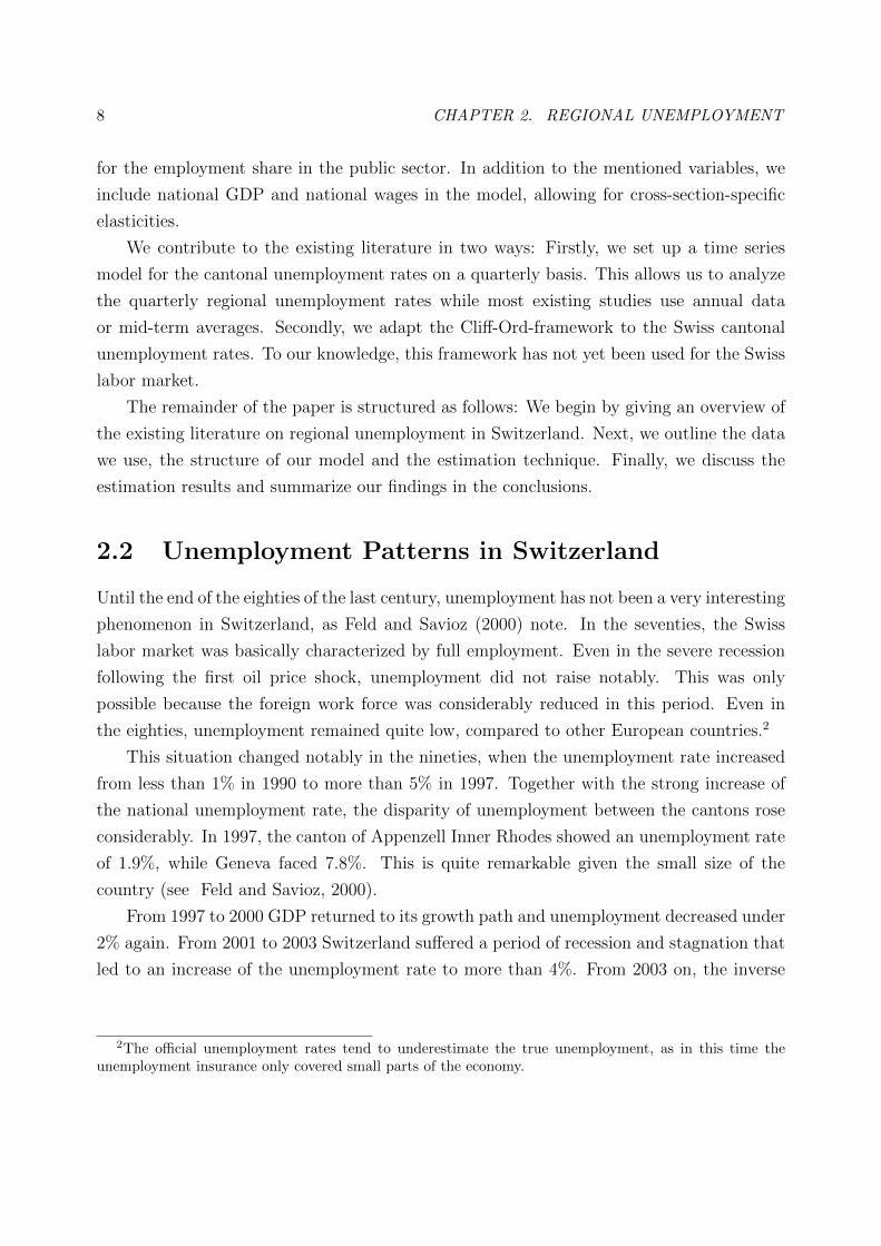
The Gini coefficient is plotted together with the Swiss unemployment rate in Figure 2.2.
In periods of high unemployment, the Gini coefficient shows smaller values than in periods
of low Swiss unemployment. This means that there is a clear tendency towards an equal
distribution in periods of high unemployment.3
In contrast, Filippini and Rossi (1992, 1993) observe a rising disparity in periods of high
unemployment. These studies analyze the standard deviation of the cantonal unemployment
instead of the Gini coefficient. There are two problems with this approach: Firstly, Filippini
and Rossi (1992) just compare the values for 1976, 1984 and 1991. Secondly, the standard
deviation highly depends on the level. The Gini coefficient also depends on the level, but
not as heavily as the standard-deviation: If all data values are doubled, the Gini coefficient
remains unchanged while the standard-deviation is doubled as well. When looking at the
3The same can be shown using the Theil index instead of the Gini coefficient.

10 CHAPTER 2. REGIONAL UNEMPLOYMENT
Figure 2.1: Swiss Unemployment Rate, Total, German- and French/Italian-Speaking Part.
Time
Per
cent
1990 1995 2000 2005 2010
01
23
45
67
SwitzerlandGerman PartsFrench and Italian Parts
Note: The unemployment rate in the French and Italian speaking cantons has been permanentlyhigher than in the German speaking cantons since 1990.
2.2. UNEMPLOYMENT PATTERNS IN SWITZERLAND 11
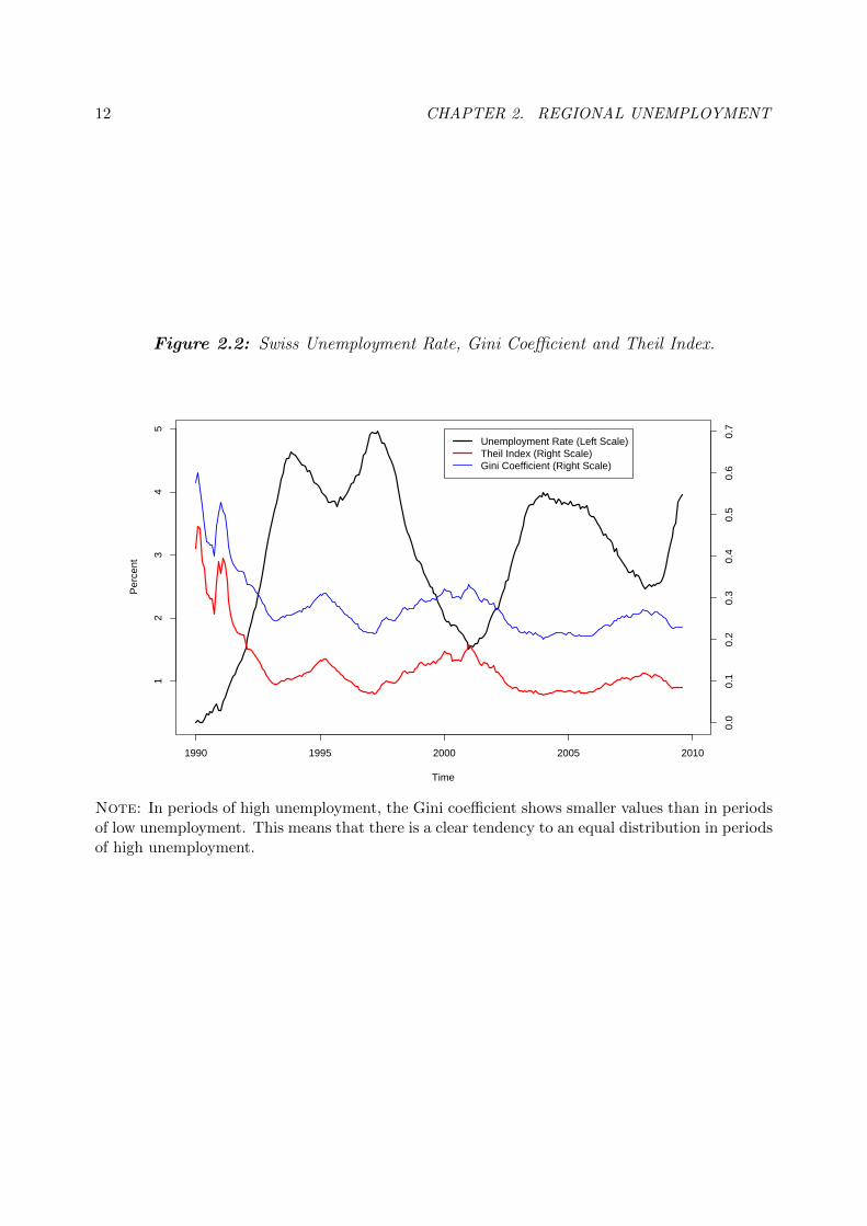
coefficient of variation, the mean-corrected standard-deviation, (see Figure 2.3) we see that
the variation is smaller in times of high unemployment rates. This is perfectly in line with
what we found analyzing the Gini coefficient.
Besides the existence and extent of regional disparities, also the determinants of the
cantons’ individual levels of unemployment have been analyzed. Starting from the works
of Lewin (1983), Filippini and Rossi (1992, 1993) and Projer (1993) many studies about
Swiss regional unemployment rates have been published in the last 10 years. While some
of them (see, e.g., De Coulon, 1999, Feld and Savioz, 2000) examine regional Beveridge
Curves, others look at in- and outflows of unemployment rather than unemployment rates
(like Fluckiger et al., 2002, Fluckiger and Vassiliev, 2002) and estimate duration models.
De Coulon (1999) and Fluckiger et al. (2002) calculate Beveridge Curves for the Swiss
Cantons. Furthermore, De Coulon (1999) analyzes the link between foreign population
and regional unemployment and shows that the regional differences in unemployment in
Switzerland are higher than in other European countries. The share of foreign residents can
partly explain these differences. While, in his estimations, the number of seasonal workers,
cross-border commuters and persons with an annual permit are not able to explain the
differences, it’s the share of foreigners with a permanent residence permit that helps to
explain the regional differences.
Fluckiger et al. (2002), Fluckiger and Vassiliev (2002) focus on the differences between
the Canton of Geneva and the other cantons. They divide the unemployment into structural,
frictional and cyclical unemployment. The analysis of micro data enables them to calculate
in- and outflows of unemployment. They hence find the smaller outflow from unemployment
to be one of the reasons for the higher unemployment rates in Geneva. By estimating
duration models, they find the duration of unemployment to be higher in Geneva than in
other cantons.
Feld and Savioz (2000) estimate a dynamic panel model. They use a model similar to
De Coulon (1999), but add different categories of explanatory variables to it. They criticize
that variables related to the cantonal economic policy or the skills of the active population
have not been analyzed in Swiss studies. In their estimations, they find high tax burdens
and the number of foreign workers to increase cantonal unemployment, while human capital
reduces unemployment.
Parnisari (2003) examines the dispersion of unemployment over time. He calculates the
Gini coefficient over time and finds the cantonal disparities to augment in times of booms.
For the 1980–1990 period, this behavior of cantonal differences is explained by a strong
12 CHAPTER 2. REGIONAL UNEMPLOYMENT
Figure 2.2: Swiss Unemployment Rate, Gini Coefficient and Theil Index.
Time
Per
cent
1990 1995 2000 2005 2010
12
34
5
Unemployment Rate (Left Scale)Theil Index (Right Scale)Gini Coefficient (Right Scale)
0.0
0.1
0.2
0.3
0.4
0.5
0.6
0.7
Note: In periods of high unemployment, the Gini coefficient shows smaller values than in periodsof low unemployment. This means that there is a clear tendency to an equal distribution in periodsof high unemployment.

2.2. UNEMPLOYMENT PATTERNS IN SWITZERLAND 13
Figure 2.3: Swiss Unemployment Rate, Standard Deviation, and Coefficient of Variation.
Time
Per
cent
1990 1995 2000 2005 2010
01
23
45
Unemployment Rate (Left Scale)Standard Deviation (Left Scale)Coefficient of Variance (Right Scale)
0.0
0.5
1.0
1.5
Note: The variation is smaller in times of high unemployment. This is perfectly in line with whatwe found analyzing the Gini coefficient.

14 CHAPTER 2. REGIONAL UNEMPLOYMENT
cyclical component and different structural components in the different cantons. For the
second phase, 1990–2002, the reason given is the rise of structural unemployment in large
parts of the cantons.
Steffen (2005) focuses more on the institutional settings for explaining the differences in
the cantonal unemployment rates. She shows that cyclical variables can explain the national
level of unemployment, but are not able to explain the different values in the cantons.
Political-institutional variables on the other hand can explain the different responses of
the cantons to the cyclical framework. Therefore, she concludes that the macroeconomic
framework does not have a direct influence on unemployment.
Brugger et al. (2007) examine how unemployment rates behave at borders. They analyze
language borders as well as country borders and are thus able to distinguish institutional
from cultural differences. Using micro data they are able to estimate entering and quitting
probabilities of unemployment. They find differences in the unemployment rate at two
types of borders: At the Swiss language borders, the differences are due to disparities for in-
and outflow of unemployed people, while at the national border between Switzerland and
Austria, differences occur in the inflows only.
Fluckiger et al. (2007a, the extended version of Fluckiger et al., 2007b) is a comprehen-
sive study discussing a wide range of approaches and combining macro- and microeconomic
approaches. Similar to Parnisari (2003) the authors calculate the Gini coefficient and find
cantonal differences to widen in economic boom phases. By calculating in- and outflows
as well as duration models, they discover that younger people have a higher probability of
becoming unemployed, but their duration in unemployment is shorter, while older people’s
probability is smaller, but the average duration is longer.
In this article, we assume the unemployment rates of the cantons to be spatially (and
temporally) correlated. We investigate which variables determine the cantonal levels of
unemployment and whether they also help to explain the differences in the spatial model.
2.3 The Data
2.3.1 The Dependent Variable
We analyze the cantonal unemployment rates. However, cantonal borders are not neces-
sarily congruent with the borders of regional labor markets. Cantons as Basel-Stadt and
Basel-Land are probably one labor market, as many people working in Basel-Stadt live in
Basel-Land. A drawback of this rather politically motivated partitioning is the fact that

2.3. THE DATA 15
cantons are often heterogenic entities. The economic, geographic and demographic charac-
teristics can vary notably inside a canton. By analyzing cantons as entities, these variations
get lost, leading to a distortion of the estimation results as actually separated labor markets
are merged.4 An important reason in favor of analyzing cantonal data is the fact that the
Swiss cantons have relatively large competences in economic and job market policy and
thus, the political and institutional environment mainly depends on the cantons. Accord-
ingly, regional data is available for the cantons (the NUTS-3 regions) or groups of cantons
(“statistical regions”, the NUTS-2 regions). The statistical regions do not have any political
autonomy; therefore the analysis of cantonal data is the best choice.
As unemployment rates show strong seasonal characteristics we use the seasonally ad-
justed series.5
2.3.2 The Independent Variables
The explanatory variables used in the relevant literature can be parted in four groups. The
first group covers information about the population structure; the second group contains
variables on the labor force; the third group covers institutional and structural information
about the regional entities; the fourth group contains macroeconomic variables.
For the population structure, we include the population density (Feld and Savioz, 2000,
Steffen, 2005), variables on the age structure (Elhorst, 2003, Feld and Savioz, 2000) and the
share of women (Fluckiger et al., 2007a, Filippini, 1998) and foreigners in the population
in our model. For the foreigners, different variables have been proposed in the literature,
namely the number of persons staying for one year, seasonal workers, foreign resident pop-
ulation and cross-border commuters. All of the mentioned studies use at least one of these
categories of foreign workers. Data is available for all these categories, but as we need re-
gional time series, we use the share of cross-border commuters in the working population,
as proposed by Fluckiger et al. (2007b), Parnisari (2003), Feld and Savioz (2000), Steffen
(2005), De Coulon (1999), Fluckiger and Vassiliev (2002).
From the second group which contains information about the labor force, we cannot
include any variables due to data availability. Variables used in the literature include the
share of unemployed persons that are in so called labor market procedures (“arbeitsmark-
tlichen Massnahmen”, Fluckiger et al., 2007b), the share of unemployed people that are
4For a deeper discussion of this, see Spiezia (2003).5We use an additive X12 procedure with the seasonal filter option X11.

16 CHAPTER 2. REGIONAL UNEMPLOYMENT
under sanctions of the unemployment insurance (Fluckiger et al., 2007b, Steffen, 2005), the
share of unemployed people that are registered (Fluckiger et al., 2007b, Parnisari, 2003,
De Coulon, 1999), labor market participation (Parnisari, 2003, Elhorst, 2003, Steffen, 2005,
De Coulon, 1999, Fluckiger and Vassiliev, 2002), the share of part time workers (Steffen,
2005, Fluckiger and Vassiliev, 2002) or the share of temporary workers (Parnisari, 2003).
All these variables are not available as regional time series and thus not included in this
analysis.
Institutional and structural information about the cantons is contained in the third
group of variables. We include in this context the employment shares of the three sectors
(Steffen, 2005), of the public sector (Steffen, 2005) and of the traditional, modern and
high tech industries as well as the dispersion of employment over industries (Elhorst, 2003,
Steffen, 2005, Parnisari, 2003, Filippini, 1998). Moreover, we considered the overall tax
burden (Feld and Savioz, 2000, Steffen, 2005) but abstained from including it as it did not
show significant explanatory power. The literature has furthermore proposed the strength of
the unions (Elhorst, 2003, Steffen, 2005) or variables on the regional administration (public
earnings, total expenditures, expenditures for education, expenditures for interests). As
there are no sufficiently long and disaggregated time series available for these variables,
they are not included in our estimations.
With regard to macroeconomic variables, we use GDP and wages. GDP is an important
determinant of unemployment as it measures the overall economy’s need for labor. But
as regional time series of economic prosperity or income which are usually proposed in the
literature (Elhorst, 2003, Feld and Savioz, 2000, Steffen, 2005, Filippini, 1998) are too short,
we use the national GDP instead. The wage level represents the price of labor and has been
used in many studies (Elhorst, 2003, Steffen, 2005, Filippini, 1998). As there are no cantonal
time series on the evolution of wages, we use national time series as well. In turn, we allow
the cantons to have individual elasticities to GDP and wages.
2.3.3 The Weighting Matrix
The weighting matrix W specifies the structure and intensity of the spatial effects. For a
set of N regions, it is an N × N matrix whose diagonal elements are set to zero. Hence,
the element wij represents the intensity of effects between two regions i and j (see, e.g.,
Anselin and Bera, 1998). The literature knows different approaches for specifying these so
called spatial weights. The most frequently used weight specifications are the binary and
the distance decay weights.

2.3. THE DATA 17
In the binary weighting matrix, wij = 1 if the regions i and j have a common border,
and wij = 0 otherwise (see, e.g., Schanne et al., 2008, Kosfeld and Dreger, 2006). The
distance decay function is based on the distance between the centers of the regions and
takes the inverse or applies a negative exponential function to it (see, e.g., Schanne et al.,
2008, Brugger et al., 2007). Simulation studies by Florax and de Graaff (2004), have shown
that a combination of these specifications can be promising: When two regions, i and j
have a common border, wij is the inverse or a negative exponential function of the distance
between their capitals, otherwise, wij = 0 (see, e.g., Buttner, 1999, Longhi and Nijkamp,
2007).
However, all these metrics are unable to represent the complex geographic structure of
the Swiss cantons. For modeling the relatedness of Swiss cantons and their labor markets,
we need more than pure geographical information. Two cantons may be close to each other,
but because of geographical obstacles – such as mountains or lakes – their labor markets
may be quite separated. This is why the binary and the distance decay specification are not
suitable in modeling Swiss cantonal data.
Instead, we use the travel times between the canton’s capitals by public transport to
construct the W -matrix. We therefore set
w∗ij =1
ttij
where ttij is the travel time from region i’s capital to region j’s capital. One could argue that
the travel times can only be calculated for these specific cities and not for the cantons them-
selves. Regional capitals can be very far from each other, but due to a large common border,
the interaction between the cantons can be quite intensive. We therefore also construct an
alternative weighting matrix using all regional capitals and all cities with more than 30’000
inhabitants. The travel times between the cantons is then calculated as weighted means of
the travel times of all included cities of the cantons. This alternative W -matrix is then used
to check the robustness of our estimation results. The resulting estimation results are very
similar to those resulting from the original W -matrix.
To facilitate the interpretation and computation of the spatial autocorrelation, the
weighting matrix is row-normalized (see, e.g., Kelejian and Robinson, 1993, Anselin and
Rey, 1991):
wij =w∗ij∑Nj=1w
∗ij
18 CHAPTER 2. REGIONAL UNEMPLOYMENT
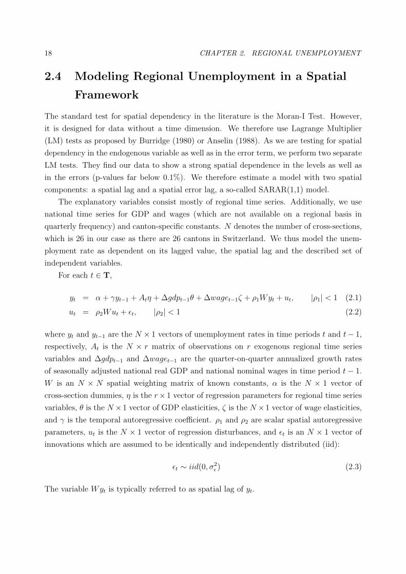
2.4 Modeling Regional Unemployment in a Spatial
Framework
The standard test for spatial dependency in the literature is the Moran-I Test. However,
it is designed for data without a time dimension. We therefore use Lagrange Multiplier
(LM) tests as proposed by Burridge (1980) or Anselin (1988). As we are testing for spatial
dependency in the endogenous variable as well as in the error term, we perform two separate
LM tests. They find our data to show a strong spatial dependence in the levels as well as
in the errors (p-values far below 0.1%). We therefore estimate a model with two spatial
components: a spatial lag and a spatial error lag, a so-called SARAR(1,1) model.
The explanatory variables consist mostly of regional time series. Additionally, we use
national time series for GDP and wages (which are not available on a regional basis in
quarterly frequency) and canton-specific constants. N denotes the number of cross-sections,
which is 26 in our case as there are 26 cantons in Switzerland. We thus model the unem-
ployment rate as dependent on its lagged value, the spatial lag and the described set of
independent variables.
For each t ∈ T,
yt = α + γyt−1 + Atη + ∆gdpt−1θ + ∆waget−1ζ + ρ1Wyt + ut, |ρ1| < 1 (2.1)
ut = ρ2Wut + εt, |ρ2| < 1 (2.2)
where yt and yt−1 are the N × 1 vectors of unemployment rates in time periods t and t− 1,
respectively, At is the N × r matrix of observations on r exogenous regional time series
variables and ∆gdpt−1 and ∆waget−1 are the quarter-on-quarter annualized growth rates
of seasonally adjusted national real GDP and national nominal wages in time period t− 1.
W is an N × N spatial weighting matrix of known constants, α is the N × 1 vector of
cross-section dummies, η is the r× 1 vector of regression parameters for regional time series
variables, θ is the N ×1 vector of GDP elasticities, ζ is the N ×1 vector of wage elasticities,
and γ is the temporal autoregressive coefficient. ρ1 and ρ2 are scalar spatial autoregressive
parameters, ut is the N × 1 vector of regression disturbances, and εt is an N × 1 vector of
innovations which are assumed to be identically and independently distributed (iid):
εt ∼ iid(0, σ2ε ) (2.3)
The variable Wyt is typically referred to as spatial lag of yt.

2.4. MODELING REGIONAL UNEMPLOYMENT IN A SPATIALFRAMEWORK 19
We next define Xt = (IN , yt−1, At,∆gdpt−1IN ,∆waget−1IN) and β = (α′, γ, η′, θ′, ζ ′)′,
where IN denotes the identity matrix of dimension N . The model then reads as follows for
each time period t:
yt = Xtβ + ρ1Wyt + ut (2.4)
ut = ρ2Wut + εt (2.5)
Xt has dimension N × k and β has dimension k × 1, where k = 3N + r + 1. We now use
stacked matrix notation to write our model in a more compact form, i.e. we stack the cross-
section data for all time periods T in matrices or vectors. For example, the N × 1 vectors
yt which contain the cross-sectional data for each time period are stacked into the NT × 1
vector y which contains the cross-sectional data for all time periods. In order to create
an NT × NT matrix containing the W matrix for all time periods, we use the Kronecker
product to define WNT = IT ⊗W , where IT denotes an identity matrix of dimension T . The
model then reads as follows:
y = Xβ + ρ1WNTy + u (2.6)
u = ρ2WNTu+ ε (2.7)
Some spatial studies assume that the dependent variable in a cross-section depends on
the values of the dependent variable in other cross-sections at time t − 1 (and not in time
t, see, e.g., Giacomini and Granger, 2004). In our model, it is more reasonable to assume
that unemployment in one canton depends on unemployment in other cantons at the same
time. When unemployment arises from a firm closing in region i, people commuting from
other regions get unemployed in the same time period as people living in region i.
Several techniques for estimating models including spatial lags and spatial error lags have
been proposed. We use the three-step procedure described by Kelejian and Prucha (1998)
as it requires relatively weak assumptions and involves lower computational complexity.
Although Kelejian and Prucha presented this model for cross-sectional data, it can easily
be adapted for time series (see, e.g., Anselin et al., 2008).
The first estimation step consists of a regression according to equation (2.6). As WNTy
is endogenous in this setting, the estimation is performed by two-stage least squares. As
instruments, denoted by H, the set (X,WNTX,W2NTX) is used. This regression produces
the estimators β and ρ1, which are consistent but not efficient, as they do not take into

20 CHAPTER 2. REGIONAL UNEMPLOYMENT
account the dependencies in the errors. The residuals u are used as estimators for the
disturbances u.
In the second step, we use u to estimate the autoregressive parameter ρ2 by a gen-
eralized moments procedure, which is outlined in appendix 2.A.3. The underlying idea
is to transform equation (2.7) repeatedly in order to create a system of equations and to
use assumption (2.3) to substitute certain terms. By solving the system of equations, the
estimators ρ2 and σε can be attained.
For the third step, equation (2.6) is premultiplied by ρ2WNT and then subtracted from
its initial version:
y − ρ2WNTy = Xβ − ρ2WNTXβ + ρ1WNTy − ρ1ρ2W2NTy + u− ρ2WNTu (2.8)
setting y∗ = y − ρ2WNTY , X∗ = X − ρ2WNTX and substituting ε for u− ρ2WNTu, we
get
y∗ = X∗β + ρ1WNTy∗ + ε (2.9)
We now have a model with iid disturbances which we can efficiently estimate by two-
stage least squares. The regression produces the final estimators β and ρ1.
Kelejian and Prucha (1998) call this step feasible spatial generalized two-stage least
squares as the theoretical value of ρ2, which is needed to calculate y∗ and X∗, is not known
but estimated.
2.5 Empirical Application to Swiss Data
This sections presents the estimation results (section 2.5.1), compares the fit of the spatial
model to alternative models (section 2.5.2) and discusses the spatial dispersion of a shock
(section 2.5.3).
2.5.1 Estimation Results
In this section, we will present the estimation results and show how they fit into the literature
and the relevant theory. The estimation was performed using quarterly data from 1998 to
2007. The detailed estimation results can be found in Table 2.4 in the appendix. This table
contains the results for four alternative models. The “Non-Spatial Model” is the starting

2.5. EMPIRICAL APPLICATION TO SWISS DATA 21
point of our analysis as it shows which variables explain the cantonal unemployment rates
without the inclusion of spatial elements. The variables showing significance are used in
the initial spatial model (“Full Model”). The final spatial model (“Selected Model”) results
by removing the insignificant variables from the full spatial model. Furthermore, the table
shows the estimated parameters of the final spatial model when excluding Basel-Stadt and
Geneva from the sample (“Robustness Check”).
Non-Spatial Model
The non-spatial model neglects the spatial dependency between the cantons and can thus
be estimated by OLS. Nevertheless, the estimated coefficients are quite similar to those of
the spatial model. In general, the coefficients are larger than in the spatial model. This is
what we would expect as the information contained in the spatial lag (which has a positive
mean) is distributed on the other explanatory variables.
Lags in Space and Time
Most studies about (regional) unemployment include a temporal lag of unemployment to
their set of explanatory variables and a small number of studies furthermore includes a
spatial lag. According to Elhorst (2003) there is mainly a statistical matter to do so.
Usually, unemployment rates are highly correlated across time and space and normally
change by relatively small amounts from period to period. As the economic situation in
adjacent regions is similar, unemployment rates tend to be correlated in space.
But besides the statistical matter, there is also an economic motivation for including the
spatial lag into the estimation system: In a small economy as Switzerland, many employees
do not work in the same canton as they live: 57% of the employees do not work in the
same community, 12% not in the same canton as they live (results from the population
census 2000). When a firm closes, employees from this region, but also from other regions
lose their jobs. Furthermore, an unemployed person living in a region also looks for a job
in other regions. These two channels cause further spatial interdependencies between the
unemployment rates of Swiss cantons. We assume the amount by which the unemployment
rate in region i is affected by the unemployment rate in region j to be proportional to the
travel times between these two regions and form our W -matrix accordingly.
In our estimations, the coefficients of the temporal and the spatial lags are all highly
significant and positive. The coefficient of the temporal lag is 0.81 and the coefficients for the
spatial lags in the dependent variable and in the error term are 0.18 and 0.64, respectively.
22 CHAPTER 2. REGIONAL UNEMPLOYMENT
While both spatial lags turn out to be significant, the dependency in the error term seems
to be even stronger than the one in the level. This is in line with the finding of Parnisari
(2003) stating that spatial correlation is stronger for the cyclical than for the structural
component of unemployment.
Women
In their study about Swiss regional unemployment, Fluckiger et al. (2007a) find the share
of women in the population to be positively correlated with the unemployment rate. Their
explanation is that after maternity, women have trouble in getting back to working life and
stay unemployed for a longer period than men. Filippini (1998) supposes that another reason
for the higher unemployment risk of women lies in the fact that the average qualification
is lower for women than for men. We can see from national statistics that the average
educational attainment is indeed lower for women than for men. But as we will see for other
variables, we do not have this data for Switzerland on cantonal level and therefore do not
include it into our estimations.
In line with to Fluckiger et al. (2007a), we find the share of women in the population
to increase cantonal unemployment.
Cross-Border Commuters
The expected effect of immigration on regional unemployment is not straightforward, as it
can increase both labor supply and demand. The effect on unemployment is zero, if migrants
fill vacancies for which no one in the home region is qualified. If migrants fill jobs for which
also domestic people are qualified, unemployment increases. The effects on labor demand
work indirectly via an increased demand for goods and services.
Cross border commuters come to Switzerland only for work and live abroad. They
tend to spend more income in their home regions than in their work regions. Therefore,
the effects on labor demand are weaker than for migrants. For migrants, the labor supply
side is usually assumed to dominate the labor demand side (see, e.g., Oud et al., 2008).
For cross-border commuters the supply side should consequently dominate the demand side
even more clearly.
For Switzerland, there are no regional quarterly time series of migration. What we
do have at hand are quarterly time series of cross-border commuters on a cantonal level.
Cross-border commuters are an important phenomenon in Switzerland. All in all, they only
account for about 2% of the working population. But when analyzing cantonal data, we

2.5. EMPIRICAL APPLICATION TO SWISS DATA 23
find large variance in the share of cross-border commuters. Not surprisingly, border cantons
are confronted with more cross-border commuters, while cantons without borders hardly
receive any of them. In Basel-Stadt and Geneva, the number of cross-border commuters
accounts for more than 10% (Geneva) or even more than 15% (Basel-Stadt) of the canton’s
working population. These two cantons are furthermore very small (Basel is the smallest,
Geneva the fifth-smallest) and the most urban ones. Their population density is more than
25 (Geneva) and 8 (Basel) times the national population density of Switzerland. This all
makes these two cantons particular and different from other cantons. Therefore, Fluckiger
and Vassiliev (2002) analyze the differences in unemployment in these two cantons compared
to the rest of Switzerland. In our model, these two cantons are modeled in the same way as
all other cantons; their particularity is mainly captured by their high number of cross-border
commuters and population density. Additionally, we run a robustness check by estimating
the model without Basel-Stadt and Geneva.
In a very simple model, Filippini and Rossi (1992) have shown that the number of
cross-border commuters has a significant positive effect on the unemployment rate. In a
later study, Fluckiger et al. (2007b) have concluded that unemployment is higher in border
regions. They explain this fact by the higher competition for vacancies in these regions,
which decreases the probability to become re-employed and thus increases the unemploy-
ment rate. They emphasize that cross-border commuters do not cause unemployment, but
make re-entrance to working life more difficult. Of course, this effect does not work in one
direction only. The working potential of foreigners increases the labor supply in Swiss border
regions. But the labor supply in foreign border regions is also affected by the Swiss working
potential. Similarly to the emergence of domestic spatial effects, this leads to an equaliza-
tion of the unemployment rates in neighboring regions on an international level. As the
unemployment rates are generally higher in Switzerland’s neighboring regions than in the
Swiss border regions, the number of cross-border commuters should increase unemployment
in Switzerland.
In our estimations we indeed find a positive effect of cross-border commuters on the
regional unemployment rates. This is perfectly in line with the above mentioned literature.
Furthermore, our robustness check shows that this result is not dominated by Basel-Stadt
and Geneva as the coefficient is virtually unchanged when these two cantons are excluded
from the sample.

24 CHAPTER 2. REGIONAL UNEMPLOYMENT
Age Structure
Several studies add variables about the age structure of the population to their set of
explanatory variables. Most of them find that regions with a relatively young population
are confronted with a more severe unemployment problem than regions with a relatively old
population (Hofler and Murphy, 1989, Johnson and Kneebone, 1991, Elhorst, 1995, Molho,
1995a,b, Partridge and Rickman, 1995).
As has been shown by Oud et al. (2008) with German data, changes in the age struc-
ture towards a younger population lead to higher, and more persistent unemployment rates.
Looking at Spanish data, Lopez-Bazo et al. (2002) find unemployment rates of people aged
16–25 to be notably higher than for the total population. And consequently, the unemploy-
ment rates of regions with a large share of people in this cohort tend to be higher.
For Switzerland, things are different. From 1990 to 2004, the unemployment rate of
the cohort 15–19 years has always been lower than for any other cohort (see Figure 2.4).
Compared to other countries, the unemployment rate for this cohort is very low. In the
European Union, unemployment among young people is measured in the cohort until 25
years and is thus not entirely comparable to Switzerland. Due to the different systems of
industrial training in the different countries, it is furthermore difficult to find the correct
age categories for comparison. Nonetheless, it can be said that in the European Union
unemployment among young people is much higher than for total population. In the last
years, the unemployment rate of people below 25 years was twice the rate for the total
population and usually between 15% and 20% (cf. Eurostat, 2009).6
In their study about Switzerland, Fluckiger and Vassiliev (2002) have shown that the
probability of losing the job is higher for younger people compared to the total population.
On the other hand, the average duration of unemployment is much shorter for younger
people.
As we would expect from the above argumentation, Feld and Savioz (2000) showed that
the higher the number of young people in a canton, the lower is unemployment. They
suppose that this could be a human capital effect.
We include the share of people in the following age categories into our estimations: 20–
24 years and 25–64 years. The base line category is therefore people aged under 20 years and
people aged over 64 years. The shares of 20–24 years and 25–64 years old people both have
6In Germany and Austria – where roughly comparable industrial training programs exist – the differencesbetween the age categories were not as high, while in France and Italy this ratio was even larger than 2.

2.5. EMPIRICAL APPLICATION TO SWISS DATA 25
Figure 2.4: Swiss Unemployment Rates in Different Age Cohorts.
Time
Per
cent
1990 1995 2000 2005 2010
01
23
45
67
Total15−19 Years20−24 Years25−64 Years
Note: From 1990 to 2004, the unemployment rate of the cohort 15–19 years has always beenlower than for any other cohort. On the other hand, the unemployment rate of the 20–24 years oldpeople was higher than in the other cohorts. Due to unstable seasonal patterns, the trend cyclesare shown.

26 CHAPTER 2. REGIONAL UNEMPLOYMENT
a significant positive effect on regional unemployment. We see two reasons for the fact that
both coefficients are positive: firstly, with the exception of the 15–19 years old people, the
former two age categories cover those people who are actually able to register as unemployed.
Thus, it makes sense that a higher population share of these cohorts should in principle
increase the unemployment rate. Secondly, we already mentioned that the only age category
which can furthermore register as unemployed, namely the 15–19 years old, experience a
lower-than-average unemployment rate. This age category was included in earlier versions of
our model and its coefficient was actually negative, although not significantly. Nevertheless,
compared to the 15–19 years old, the 20–24 and 15–64 years old people experience higher
unemployment rates, and thus unemployment should rise with their population share. When
comparing the coefficients of the included age categories, we see that the coefficient of the
20–24 years old is higher than the one for the 25–64 years old. This reflects the fact that
the 20–24 years old people experience a clearly higher-than-average unemployment rate.
Sectoral Employment
The effects of the sectoral employment mix on unemployment are not a priori clear, as
different argumentations are possible. This is reflected in the mixed results of including the
sectoral employment shares (Elhorst, 1995, Partridge and Rickman, 1995, 1997, Taylor and
Bradley, 1997). Armstrong and Taylor (1993) argue that the unemployment rate is not
specific to regions, but to industries. Therefore, they explain the unemployment rate in a
specific region by its industry mix and the national rate of unemployment in each industry.
But as Martin (1997) shows, the unemployment rate of a specific industry can be different
in different regions.
An important phenomenon in the context of sectoral employment and unemployment is
the tertiarization process, which is supposed to cause unemployment to be higher in regions
specialized in agriculture and manufacturing than in regions specialized in services. As
Sheldon (1999) points out, Switzerland was confronted with a tertiarization of the working
environment since the 1960s. Employment in production and manufacturing decreased,
while the services sector showed an increase in employment and added value. Steffen (2005)
thus supposes that cantons with a large manufacturing sector have a larger number of
endangered jobs. In cantons with a large service sector, tertiarization is more advanced and
the number of endangered jobs is smaller. However, the estimations conducted by Steffen
(2005) indicate that unemployment rises with the employment share of the services sector.

2.5. EMPIRICAL APPLICATION TO SWISS DATA 27
As it seems, tertiarization is not the only channel through which the sectoral mix affects
unemployment.
An argument in the opposite direction can be made using employment multipliers. The
former are generally higher in agriculture and manufacturing than in the services sector,
given that the first two sectors – at least partly – create the demand for some services
(Elhorst, 2003). Consequently, unemployment could fall with the employment shares of the
first two sectors. With regard to the first sector, the following argumentation can addition-
ally be made: enterprises in the agriculture sector are frequently family enterprises. If a
family member loses his/her job outside the farm, he/she often can work on the farm and
does not register as unemployed. Furthermore, social control is rather strong in regions with
a high employment share of the first sector, i.e. people who lost their job may register less
frequently as unemployed than in other regions because they feel ashamed. A high employ-
ment share of the first sector could thus dampen unemployment not through economic, but
through psychological mechanisms.
In our study, we would not expect tertiarization to play a dominant role as we use data
from 1998 to 2007. Figure 2.5 shows that the process of tertiarization was quite advanced in
1998. Although the employment shares changed further during our sample, the main part of
the evolution was already completed. With respect to the second sector, we can furthermore
say that those industries that still produced in Switzerland in 1998 were mainly high tech
industries. They may have a rather high employment multiplier and be less affected by
tertiarization.
Similar to Oud et al. (2008), we measure the economic structure as the proportion of
employment in agriculture, manufacturing and services. In our estimations, we include
the shares in employment of the second and the third sector in the explanatory variables.
While the coefficient of the second sector is not significant (and thus not reported), the
coefficient of the third sector is positive. A higher employment share of the third sector
therefore increases unemployment. We thus conclude that tertiarization does indeed not
dominate our result. Instead, higher employment multipliers, robust industries, familial job
opportunities and social control seem to decrease unemployment in the first and the sector
sector.
Besides the breakdown into the three sectors, we also analyze the internal structure of
the modernity of the industries and discriminate three stages: traditional, modern and high-
tech industries. The share of employment in traditional industries is supposed to increase
unemployment as the former are generally declining. On the other hand, the employment

28 CHAPTER 2. REGIONAL UNEMPLOYMENT
Figure 2.5: Employment Shares of the Sectors.
Time
Em
ploy
men
t Sha
res
1960 1970 1980 1990 2000
0.1
0.2
0.3
0.4
0.5
0.6
0.7
1st sector2nd sector3rd sector
Note: The dotted line shows 1998, the begin of our sample.

2.5. EMPIRICAL APPLICATION TO SWISS DATA 29
share of high-tech industries should decrease unemployment as these are only little affected
by structural change. The same argument can be mode for modern industries. Surprisingly,
we only find a significant effect for the modern industries: the higher the share of employment
in modern industries, the higher is unemployment. We explain this result with the bursting
of the “dot-com-bubble”, which falls into our estimation sample and caused unemployment
among bankers and IT engineers to increase considerably. As modern industries mainly
include the financial sector and IT, this one-time shock could explain our result.
Industrial Concentration
Industrial diversity – the opposite of industrial concentration – is the dispersion of employ-
ment over industries. Several studies suggest that it is negatively related to unemployment.
The idea is that regions with multiple sources of employment provide more chances to be-
come re-employed. Elhorst (2001) cites five studies investigating the relationship between
unemployment and industrial diversity (Taylor and Bradley, 1983, Neumann and Topel,
1991, Malizia and Ke, 1993, Simon, 1988, Partridge and Rickman, 1995). All of them find
the expected effect. However, it is significant in the first three studies only. On the other
hand, one might also argue that concentration in employment is a sign for industrial clus-
tering, which leads to network effects. These can lower unemployment.
The dispersion of employment over the industries is measured by the Herfindahl index.
Originally developed to measure the amount of competition among firms, it has undergone
several adaptions for other purposes. The idea is to calculate an index of the concentration
of output over firms, employment over industries etc. It is calculated as H =∑N
i=1 s2i with
N : number of industries, si: share of employment in industry i. It reaches a maximum of
1 in the case of total concentration of employment in one industry. Smaller values indicate
more equally distributed employment.
For Switzerland, Filippini (1998) assumes economies with a larger dispersion of em-
ployment to show more stable GDP growth and lower unemployment rates than economies
specialized in fewer industries. This is confirmed by the findings of Steffen (2005). In con-
trast, we find a concentration of employment in few industries to lower unemployment. The
benefits of clustering seem to dominate the gains of diversification. The differences to the
results of the above cited studies may be due by the varying samples used.
This effect only exists in the non-spatial setting. When including spatial elements, the
effect of industrial concentration is not significant any more.

30 CHAPTER 2. REGIONAL UNEMPLOYMENT
Public Sector
As stated by Steffen (2005), the share of employment of the public sector is assumed to have
a dampening effect on unemployment. The argument for this is twofold: Firstly, the public
sector is less affected by economic crises (see Forni, 2002), and secondly, the enlargement
of public employment in times of economic crises can dampen the raise in unemployment
(Armingeon, 1999). Other studies (see, e.g., Parnisari, 2003) put it another way and state
that a large share of employment in industries with a low responsiveness to the business
cycle lower the variance of unemployment.
Steffen (2005) includes the share of employment of the public sector in her models. She
cannot find a significant effect in any of the estimated models. In contrast to Steffen (2005),
but in line with the above mentioned theory, we find a slight, but negative effect.
Population Density
Population density is often taken as a proxy for the market potential of a region. It is
sometimes called potential demand or agglomeration potential. The idea is that through
the mechanisms of economies of scale and transport costs, firms tend to produce – and thus
demand labor – in regions with high population density. Elhorst (1995) and Molho (1995a,b)
model the regional unemployment rate as dependent on the market potential. They all find
a negative and significant effect of the market potential on the regional unemployment
rate. On the other hand, there is also an intuitive argument for the opposite direction:
unemployed people may rather move into the cities as they can benefit from the nearby
services and vacancies.
In Switzerland, population density is very different across cantons. In the two urban
cantons Basel-Stadt and Geneva it is very high while in more rural cantons as the Grisons
or Uri it is quite low. The maximum is reached by Basel-Stadt with more than 5000 people
per km2, in Geneva it is about 1500 people per km2. As we have discussed above, these
two border cantons are confronted with a large number of cross-border commuters. The
nation-wide mean population density is 187 people per km2 and the minimum lies at 25
persons per km2 in the Grisons. In general, population density is negatively correlated with
the share of persons occupied in the first sector (cf. Figure 2.6).
In our estimations, we find a significant positive effect of the population density on
unemployment. This contradicts the presented theory, but is in line with the intuition.
As mentioned, there is a high correlation with cross-border commuters in the cantons
Basel-Stadt and Geneva. As these two cantons could influence the estimates for population

2.5. EMPIRICAL APPLICATION TO SWISS DATA 31
density much, we checked the robustness by estimating our model without these two cantons.
The result is given in Table 2.4. We see that the coefficient for population density becomes
insignificant when Basel Stadt and Geneva are excluded from the sample while all other
coefficients are stable. This result is more in line with the theory than the result when
considering all cantons.
GDP
One of the most widely used variables for labor demand is the regional GDP in real terms.
The relation is assumed to be positive, i.e. we expect a negative relation to unemployment.
Feld and Savioz (2000) use cantonal GDP for explaining cantonal unemployment rates.
In their estimations, they find a negative – but insignificant – effect. Only when aggregating
the 26 cantons to seven NUTS-2 regions, the effect becomes significant. Steffen (2005) finds
a negative – and for some models even significant – effect of GDP growth on regional
unemployment. She reasons that cantonal economic growth is important for describing the
different levels of unemployment, but it is not their main determinant.
As in Switzerland there is no quarterly data for the regional GDP, we use the national
GDP instead. We include annualized quarter-on-quarter GDP growth with a lead of one
quarter and individual coefficients to our model. The coefficients can then be interpreted
as elasticities. Figure 2.7 illustrates the cantonal elasticities of the unemployment rate to
GDP. The strongest reactions are registered in Geneva, Zurich, Jura and Neuchatel. On
the other hand, only small elasticities are registered in Appenzell Inner Rhodes and Outer
Rhodes, Ticino, Obwalden and Nidwalden.
As the coefficients for the elasticity to GDP are quite similar across the cantons, we test
them on equality. The corresponding F-Test rejects the equality of equal elasticities. We
therefore need individual coefficients for GDP.
Wages
The wage level represents the price of labor and has been used in many studies (Steffen,
2005, Filippini, 1998, Burridge and Gordon, 1981, Hofler and Murphy, 1989, Partridge and
Rickman, 1995, Molho, 1995b,a, Partridge and Rickman, 1997). Wages are usually believed
to have a positive effect on labor supply and a negative effect on labor demand, hence
unemployment should increase if wages rise. Indeed, most Swiss and international studies
analyzing the effect of wages on unemployment find a positive relationship (cf., e.g., Steffen,

32 CHAPTER 2. REGIONAL UNEMPLOYMENT
Figure 2.6: Employment Share of the First Sector and Population Density.
●
●
●
●
●
●
●
●
●
●●
●
●
●●
●
●
●
●
●
●
●
●
●
5 10 15 20
020
040
060
080
0
Share of Employment of the First Sector
Pop
ulat
ion
Den
sity
Note: The values for Basel Stand and Geneva are outside the panel. They both have a smallshare of employment in the first sector and a very large population density.

2.5. EMPIRICAL APPLICATION TO SWISS DATA 33
Figure 2.7: Elasticities of Swiss Cantons to a Change in National GDP.
Note: The strongest reactions are registered in Geneva, Zurich, Jura and Neuchatel. On theother hand, only small elasticities are registered in Appenzell Inner Rhodes and Outer Rhodes,Ticino, Obwalden and Nidwalden.

34 CHAPTER 2. REGIONAL UNEMPLOYMENT
2005, Filippini, 1998, Burridge and Gordon, 1981, Hofler and Murphy, 1989, Partridge and
Rickman, 1995, 1997).
As a measure for wages, we use the wage index of the Swiss Federal Statistical Office,
which records the evolution of the national mean wage. This index excludes bonuses and
measures the change in the fees paid for given tasks. In other words, it is a good index
for the evolution of unit labor costs, rather than a general income measure. We include
annualized quarter-on-quarter growth rates of the wage index in our model. As we have no
regional data for the wage index, we allow the cantons to have individual elasticities. In line
with the above mentioned literature, we find a positive effect of the wages on unemployment
in all cantons. Figure 2.8 illustrates the cantonal elasticities of the unemployment rate to
the wages. With the exception of Jura, the Latin speaking cantons show lower elasticities
than the German ones.
Again, we conduct an F-Test to check whether we really need individual wage elasticities.
The null hypothesis of one equal coefficient is clearly rejected.
Constants
Studies analyzing the different levels in the unemployment rates across regions often use
individual constants to summarize all unobserved cross-section specific factors. An F-test
clearly indicates that these individual constants should not be summarized into one common
intercept in our model.
2.5.2 Model Fit
To evaluate how well our model fits the data, we use two benchmark models (results on the
coefficients are not reported): A model with the same exogenous explanatory variables but
without spatial components (“OLS model”) and a naive autoregressive model, containing
individual constants and a common AR-coefficient for all cross-sections (“AR model”). In
both models, the coefficient of the time lag of the dependent variable is considerably higher
than in the spatial model (OLS model: 0.90; AR model: 0.92). This is due to the high
persistence of the unemployment rates: a part of the information that was contained in the
spatial lags is now captured by the time lag.
To compare the results of the spatial model to those of the benchmark models, we
measure the in-sample fit of the three models. However, there are several possibilities of
how to fit the endogenous variable: While for the OLS model and the AR model, the

2.5. EMPIRICAL APPLICATION TO SWISS DATA 35
Figure 2.8: Elasticities of Swiss Cantons to a Change in National Wages.
Note: With the exception of Jura, the Latin speaking cantons show lower elasticities than theGerman ones.

36 CHAPTER 2. REGIONAL UNEMPLOYMENT
information to use for the fit clearly consists of the actual values of the exogenous variables
and the temporally lagged dependent variable, for the spatial model, we may furthermore
include the spatial lag (i.e., the contemporaneous values of the dependent variable). Kelejian
and Prucha (2007) present four predictors for spatial models, based on different information
sets:7
Λ1 = {Xt,W}
Λ2 = {Xt,W,wi.yt} (2.10)
Λ3 = {Xt,W, y−i,t} ,
where wi. denotes the i-th row of W and y−1,t denotes the yt vector from which the i-th
element has been removed. Information set Λ1 is thus a subset of Λ2 which again is a subset
of the full information set Λ3. The first three predictors which Kelejian and Prucha (2007)
present are the conditional means corresponding to the information sets Λp, p = 1, 2, 3, in
(2.10):
y(1)it = E(yit|Λ1)
= (I − ρ1W )−1i. xtβ (2.11)
y(2)it = E(yit|Λ2)
= ρ1wi.yt + xti.β +cov(uit, wi.yt)
var(wi.yt)[wi.yt − E(wi.yt)] (2.12)
y(3)it = E(yit|Λ3)
= ρ1wi.yt + xti.β + cov(uit, y−i,t) [V C(y−i,t)]−1 [y−i,t − E(y−i,t)] (2.13)
where VC denotes the variance-covariance matrix. Calculational details are given in Kelejian
and Prucha (2007). The fourth predictor they consider is given by
y(4)it = ρ1wi.yt + xi.tβ (2.14)
7Kelejian and Prucha (2007) define their predictors for a cross-sectional model. We adapt their predictorsfor a time series model. A fifth predictor which is presented in their paper refers to the spatial error modelwithout spatial lag in the dependent variable and is thus not adequate for our model.

2.5. EMPIRICAL APPLICATION TO SWISS DATA 37
This predictor may be seen as a restricted version of predictor y(2)it , implicitly assuming
that cov(uit, wi.yt) = 0. This does, however, not hold in general. Thus, conditional on the
information set Λ2, predictor 4 is biased. Kelejian and Prucha (2007) find that predictor 3,
which uses the full information set Λ3, empirically performs best.
To compare the predictors, we measure the goodness of fit by the root mean squared error
(RMSE) and the adjusted R2. Tables 2.1 and 2.2 show the ranks which the predictors of the
spatial model and the benchmark models reach as measured by these criteria8. Furthermore,
figures 2.9 and 2.10 show boxplots of the distribution of the model fit criteria through the
cross-sections. We see that predictors 2 and 3 of the spatial model together reach by far the
best ranks. Measured by the RMSE ranks, predictor 2 even seems to outperform predictor
3. However, the corresponding boxplots show that the RMSEs of the two predictors are
distributed similarly. The adjusted R2 indicates that the two predictors perform roughly the
same as well. This result indicates that in our context, there is no clear difference between
the information sets Λ2 and Λ3, or rather between the information contained in wi.yt and
y−i,t. In words, knowing the weighted mean of the unemployment rates in all other cantons
is roughly the same as knowing the actual unemployment rates in the other cantons. This
implies that our W matrix is a good measure for the interdependencies between the cantonal
labour markets. Behind predictors 2 and 3, predictors 4 and 1 and the OLS model follow.
The AR model, which uses the smallest information set of all predictors, clearly performs
the worst.
2.5.3 Emanating effects
We now use our model to calculate the emanating effects of a change in the explanatory
variables. We run an alternative scenario assuming a reduction of cross-border commuters
by 10% from the first quarter 2003 onwards in all cantons as compared to the actual values.
We then compare the resulting unemployment rates with the fitted unemployment rates in
our model which result using the actual values. A change as assumed in our scenario might
be caused by a more restrictive handling of border commuting. Such policies are sometimes
called for as a measure against unemployment in border cantons. A reduction of cross-
border commuters would not only influence unemployment directly in all cantons which
record cross-border commuters, but by spatial effects also indirectly in all other cantons.
8For the RMSE themselves, see Table 2.5

38 CHAPTER 2. REGIONAL UNEMPLOYMENT
Table 2.1: Root Mean Squared Error of the Different Predictors, Ranks.
Sp. Pred. 1 Sp. Pred. 2 Sp. Pred. 3 Sp. Pred. 4 OLS AR
1st 0 15 9 2 0 02nd 1 8 16 1 0 03rd 0 2 0 17 7 04th 9 0 1 6 10 05th 16 0 0 0 9 16th 0 1 0 0 0 25
Figure 2.9: Root Mean Squared Error of the Different Predictors.
●
●●
● ●
●
Sp. Pred. 1 Sp. Pred. 2 Sp. Pred. 3 Sp. Pred. 4 OLS 2 AR
0.05
0.10
0.15
0.20
0.25
0.30
0.35
Note: Predictor 2 reaches the best performance for some cross-sections, but performs worse thanpredictor 3 for some others.

2.5. EMPIRICAL APPLICATION TO SWISS DATA 39
Table 2.2: Adjusted R squared of the Different Predictors, Ranks.
Sp. Pred. 1 Sp. Pred. 2 Sp. Pred. 3 Sp. Pred. 4 OLS 2 AR
1st 0 12 11 2 1 02nd 1 12 13 0 0 03rd 0 1 1 14 8 24th 10 0 1 9 5 15th 13 0 0 1 12 06th 2 1 0 0 0 23
Note: Predictors 2 and 3 of the spatial model together reach by far the best ranks. Predictor2 even obtains the best fit more often than Predictor 3. Predictors 4 and 1 and the OLS modelfollow, while the AR model performs clearly the worst.
Figure 2.10: Adjusted R squared of the Different Predictors.
●
●
●
●
●
Sp. Pred. 1 Sp. Pred. 2 Sp. Pred. 3 Sp. Pred. 4 OLS 2 AR
0.85
0.90
0.95
1.00
Note: Predictor 2 reaches the best performance for some cross-sections, but performs clearly worsethan predictor 3 for some others. Not surprisingly, the models using less information perform worse.

40 CHAPTER 2. REGIONAL UNEMPLOYMENT
As the coefficient of the share of cross-border commuters is negative in our model, reducing
the number of cross-border commuters will ceteris paribus lower unemployment.
The emanating effects of a change in one or more explanatory variables can be calculated
by rewriting the model (2.4) as follows (see, e.g., Kelejian et al., 2008):
yt = (I − ρ1W )−1Xtβ + (I − ρ1W )−1ut (2.15)
Let (I − ρ1W )−1Xtβ be the N × 1 vector of values resulting from the actual values of
Xt. Furthermore, let (I−ρ1W )−1Xtβ|alt denote the corresponding values for our alternative
scenario. Assuming that the error terms remain unchanged, the emanating effects can then
be calculated as the difference between these values:
(I − ρ1W )−1Xtβ|alt − (I − ρ1W )−1Xtβ (2.16)
Table 2.3 shows the detailed emanating effects, i.e. the differences which result from
the reduction in cross-border commuting. The effects are listed for the yearly average
unemployment rate. The emanating effects grow over time, but the increases diminish
towards the end of the horizon. This increase over time is due to the auto-regressive structure
of our model, where the differences in one period have an impact on the differences in the
following periods. The new equilibrum lies up to 1.16 percentage point below the initial
values for Basel-Stadt, whereas almost no effect at all is visible in Uri, Schwyz and Zug.
Figure 2.11 shows the geographical dispersion of the emanating effects four years after the
change in commuting. Not surprisingly, the strongest results are registered in the border
cantons in general, and especially in Basel-Stadt, Basel-Land, Jura, Geneva and Ticino.
These five cantons record the highest share of cross-border commuters and thus experience
the highest reduction of commuters in our alternative scenario. The more centrally situated
cantons on the other hand experience small effects only. Some central cantons record no
cross-border commuters at all (and therefore no reduction in the alternative scenario) and
only experience indirect effects.
A word of caution about the results discussed here is in order. We have run an alter-
native scenario assuming that all explanatory variables except the number of cross-border
commuters remain unchanged. We would, however, expect a forced reduction in the number
of cross-border commuters to have an impact on some of the other explanatory variables.

2.6. CONCLUSIONS 41
Especially GDP could be affected negatively, which in turn would raise unemployment.
In order to determine the dynamic effects of our scenario, we would need to determine
the affected explanatory variables endogenously in the model. Therefore, our static analysis
cannot determine whether a reduction in the number of cross-border commuters would raise
or lower unemployment once all direct and indirect effects are taken into account. It should
merely be seen as an illustration of the dispersion of the immediate effects. Because of the
spatial lag in the model, the cantons that do not record cross-border commuters at all are
hit indirectly via the changed unemployment rate of other cantons.
2.6 Conclusions
In this paper, we estimate a spatial time series model for the Swiss cantonal unemployment
rates. This allows us to determine the variables which explain the levels and fluctuations
in the regional unemployment rates and investigate whether these variables retain their
explanatory power once spatial elements are added to the model. As we find spatial de-
pendency in the levels as well as in the errors, we estimate a SARAR(1,1) model. Our
estimation results indicate that spatial spillovers have additional explanatory power to our
other model variables.
Furthermore, we find that regional unemployment is raised by the population shares
of women, of cross-border commuters and of people aged between 20 and 24 as well as
between 25 and 64, by the population density, by the employment share of the third sector
and of modern industries and by wage growth. On the other hand, we find decreasing
effects by the employment share of the public sector and by GDP growth. Most of these
findings are consistent with the existing literature on regional unemployment levels. We
then compare the predictions of the spatial model to some alternative models. We see
that our spatial model reaches a better fit than a benchmark model which uses the same
explanatory variables but no spatial lags.
The possibilities of hypothesis testing with our model are restricted by the availability
of quarterly regional data. Furthermore, the data we have at hand is often disposable for
short time periods only. As data availability improves over time, expansions of our model
might well be possible in the future.

42 CHAPTER 2. REGIONAL UNEMPLOYMENT
Table 2.3: Emanating Effects for the Alternative Scenario of a Reduction in Cross-BorderCommuters.
2003 2004 2005 2006 2007
AG −0.05 −0.14 −0.24 −0.34 −0.44AI −0.02 −0.08 −0.16 −0.24 −0.34AR −0.02 −0.08 −0.15 −0.23 −0.32BE −0.02 −0.09 −0.17 −0.27 −0.37BL −0.15 −0.35 −0.51 −0.65 −0.78BS −0.32 −0.66 −0.86 −1.02 −1.16FR −0.02 −0.08 −0.17 −0.26 −0.36GE −0.17 −0.38 −0.54 −0.69 −0.83GL −0.02 −0.08 −0.15 −0.24 −0.33GR −0.05 −0.14 −0.22 −0.32 −0.41JU −0.13 −0.29 −0.43 −0.56 −0.7LU −0.02 −0.07 −0.14 −0.23 −0.32NE −0.07 −0.19 −0.3 −0.41 −0.54NW −0.02 −0.07 −0.14 −0.22 −0.32OW −0.02 −0.07 −0.14 −0.22 −0.32SG −0.04 −0.11 −0.18 −0.26 −0.36SH −0.11 −0.24 −0.35 −0.46 −0.58SO −0.03 −0.11 −0.2 −0.3 −0.4SZ −0.02 −0.07 −0.14 −0.22 −0.31TG −0.04 −0.12 −0.21 −0.3 −0.4TI −0.21 −0.44 −0.59 −0.72 −0.85UR −0.02 −0.07 −0.14 −0.22 −0.31VD −0.06 −0.15 −0.26 −0.36 −0.47VS −0.03 −0.11 −0.2 −0.3 −0.4ZG −0.02 −0.07 −0.14 −0.22 −0.31ZH −0.02 −0.09 −0.17 −0.26 −0.36
Note: Annual averages in official unemployment rates.

2.6. CONCLUSIONS 43
Figure 2.11: Emanating Effects in the Year 2007 for the Alternative Scenario of a Re-duction in Cross-Border Commuters.
Note: Annual average in official unemployment rates.

44 CHAPTER 2. REGIONAL UNEMPLOYMENT

2.A. APPENDIX 45
2.A Appendix
2.A.1 Estimated Coefficients
Table 2.4: Estimation Results.
Selected Full Robustness Non-Spatial
Model Model Check Model
Temporal Lag 0.81∗∗∗ 0.81∗∗∗ 0.82∗∗∗ 0.90∗∗∗
(0.02) (0.02) (0.02) (0.01)
Spatial Lag (ρ1) 0.18∗∗∗ 0.18∗∗∗ 0.17∗∗∗
(0.02) (0.05) (0.02)
Spatial Error Lag (ρ2) 0.64∗∗∗ 0.63∗∗∗ 0.64∗∗∗
(0.05) (0.02) (0.00)
Cross border commuters 0.09∗∗∗ 0.09∗∗∗ 0.10∗∗∗ 0.12∗∗∗
(% share in total population) (0.01) (0.01) (0.02) (0.01)
Women 0.21∗∗∗ 0.21∗∗∗ 0.21∗∗∗ 0.40∗∗∗
(% share in total population) (0.04) (0.04) (0.04) (0.05)
Population Density 0.97∗∗∗ 0.96∗∗∗ 1.43 0.68∗
(population in 1000 per km2) (0.30) (0.30) (1.20) (0.38)
Population aged 20-24 0.06∗∗ 0.06∗∗ 0.06∗∗ 0.21∗∗∗
(% share in total population) (0.03) (0.03) (0.03) (0.03)
Population aged 25-64 0.04∗∗∗ 0.04∗∗∗ 0.05∗∗∗ 0.11∗∗∗
(% share in total population) (0.02) (0.02) (0.02) (0.02)
Size of Public Sector −0.02∗∗ −0.02∗∗ −0.02∗∗ −0.05∗∗∗
(% share in FTE employment) (0.01) (0.01) (0.01) (0.01)
Industrial Concentration −3.94 −14.56∗
(4.15) (6.12)
Size of 3rd Sector 0.01∗∗∗ 0.01∗∗∗ 0.02∗∗∗ 0.04∗∗∗
(% share in FTE employment) (0.01) (0.01) (0.01) (0.01)
Size of Modern Industries 0.02∗∗ 0.02∗∗∗ 0.01∗ 0.08∗∗∗
(% share in FTE employment) (0.01) (0.01) (0.01) (0.01)
Observations 1040 1040 1040 1040
Note: Omitted variables are constants as well as GDP and wage elasticities. Standard errors inparentheses; * significant at the 90% confidence level; ** significant at the 95% confidence level;*** significant at the 99% confidence level; FTE: full-time equivalent

46 CHAPTER 2. REGIONAL UNEMPLOYMENT
2.A.2 Root Mean Sqared Error of the Different Predictors
Table 2.5: Root Mean Sqared Error of the Different Predictors.
Sp. Pred. 1 Sp. Pred. 2 Sp. Pred. 3 Sp. Pred. 4 OLS AR
AG 0.14 0.06 0.06 0.12 0.12 0.19
AI 0.15 0.10 0.10 0.14 0.14 0.15
AR 0.16 0.11 0.11 0.14 0.12 0.16
BE 0.12 0.05 0.06 0.11 0.10 0.18
BL 0.11 0.07 0.07 0.09 0.10 0.18
BS 0.15 0.09 0.09 0.13 0.15 0.22
FR 0.09 0.09 0.08 0.08 0.10 0.16
GE 0.17 0.12 0.12 0.16 0.15 0.26
GL 0.15 0.09 0.10 0.13 0.14 0.18
GR 0.11 0.09 0.08 0.09 0.10 0.14
JU 0.28 0.19 0.20 0.26 0.26 0.36
LU 0.14 0.07 0.08 0.13 0.14 0.19
NE 0.16 0.12 0.12 0.15 0.18 0.25
NW 0.10 0.07 0.07 0.09 0.13 0.14
OW 0.12 0.11 0.11 0.11 0.13 0.14
SG 0.11 0.06 0.07 0.09 0.09 0.16
SH 0.17 0.12 0.12 0.15 0.18 0.22
SO 0.20 0.12 0.12 0.18 0.18 0.27
SZ 0.11 0.07 0.07 0.10 0.13 0.16
TG 0.12 0.05 0.05 0.11 0.11 0.18
TI 0.14 0.13 0.12 0.13 0.17 0.23
UR 0.11 0.13 0.12 0.11 0.12 0.12
VD 0.13 0.10 0.09 0.12 0.14 0.22
VS 0.17 0.14 0.14 0.16 0.18 0.24
ZG 0.14 0.10 0.10 0.12 0.11 0.21
ZH 0.17 0.11 0.11 0.16 0.16 0.25
Median 0.14 0.10 0.10 0.13 0.13 0.18

2.A. APPENDIX 47
2.A.3 Generalized moments procedure
This section outlines the generalized moments procedure proposed by Kelejian and Prucha
(1998), which produces an estimator for the parameter ρ2. The point of departure are the
following transformations of equation (2.7):
u− ρ2WNTu = ε (2.17)
WNTu− ρ2W2NTu = WNT ε (2.18)
We define ui, ui and ui to be, respectively, the i-th elements of u, u = WNTu and u = W 2NTu.
Similarly, we define εi and εi to be the i-th elements of ε and ε = WNT ε. We can then write
the above equations as follows:
ui − ρ2ui = εi, i = 1, ..., NT (2.19)
ui − ρ2ui = εi, i = 1, ..., NT (2.20)
By squaring and then summing both equations, multiplying (2.19) by (2.20) and sum-
ming and finally dividing all terms by NT , the following system of equations is constructed:
2ρ21
NT
∑uiui − ρ2
2
1
NT
∑u2i +
1
NT
∑ε2i =
1
NT
∑u2i (2.21)
2ρ21
NT
∑uiui − ρ2
2
1
NT
∑u
2i +
1
NT
∑ε2i =
1
NT
∑u2i (2.22)
ρ21
NT
∑(uiui + u2
i )− ρ22
1
NT
∑uiui +
1
NT
∑εiεi =
1
NT
∑uiui (2.23)
As a next step, expectations are taken across the system and the terms involving ε
replaced as follows:
E
(1
NT
∑ε2i
)= σ2
ε (2.24)
E
(1
NT
∑ε2i
)=
1
NTσ2ε tr(W
′NTWNT ) (2.25)
E
(1
NT
∑εiεi
)= 0, (2.26)
where tr(.) denotes the trace operator. While (2.24) and (2.25) follow from assumption
(2.3), (2.26) additionally makes use of the fact that all diagonal elements of WNT are zero.
48 CHAPTER 2. REGIONAL UNEMPLOYMENT
The system of equations can now be written as follows:
Γ(ρ2, ρ22, σ
2ε )′ − γ = 0 (2.27)
where
Γ =1
NT
2E(u′u) −E(u′u) NT
2E(u′u) −E(u
′u) tr(W ′
NTWNT )
2E(u′u+ u′u) −E(u′u) 0
(2.28)
γ =1
NT
E(u′u)
E(u′u)
E(u′u)
(2.29)
The expectations are next replaced by their sample analogues using u from the two-stage
least squares regression in the first estimation step. Equation (2.27) can then be solved by
nonlinear least squares to get the estimators ρ2 and σ2ε .

Bibliography
Anselin, L. (1988). Spatial Econometrics: Methods and Models. Studies in Operational
Regional Science 4, Kluwer Academic Publishers, Dordrecht; Boston.
Anselin, L. and Bera, A. K. (1998). Spatial Dependence in Linear Regression Models
with an Introduction to Spatial Econometrics. In Handbook of Applied Economic Statistics
(U. A. Giles D, ed.). Marcel Dekker, New York, 237–289.
Anselin, L., le Gallo, J. and Jayet, H. (2008). Spatial Panel Econometrics. In The
Econometrics of Panel Data: Fundamentals and Recent Developments in Theory and
Practice (L. Matyas and P. Sevestre, eds.), 2008th ed. Advanced Studies in Theoretical
and Applied Econometrics, Springer, Berlin.
Anselin, L. and Rey, S. (1991). Properties of Tests for Spatial Dependence in Linear-
Regression Models. Geographical Analysis 23 112–131.
Armingeon, K. (1999). Politische Reaktionen auf Steigende Arbeitslosigkeit. In Nationaler
Staat und Internationale Wirtschaft (A. Busch and T. Plumper, eds.). Nomos, Baden-
Baden, 169–196.
Armstrong, H. and Taylor, J. (1993). Regional Economics and Policy. Blackwell,
Oxford.
Brugger, B., Lalive D’Epinay, R. and Zweimuller, J. (2007). Regionale Dis-
paritaten in der Arbeitslosigkeit: Kulturelle Grenzen und Landesgrenzen. Tech. rep.,
SECO.
Buttner, T. (1999). Agglomeration, Growth, and Adjustment a Theoretical and Empirical
Study of Regional Labor Markets in Germany. Physica-Verlag, Heidelberg Etc.
Burridge, P. (1980). Cliff-Ord Test for Spatial Correlation. Journal of the Royal Statis-
tical Society Series B-Methodological 42 107–108.
49

50 BIBLIOGRAPHY
Burridge, P. and Gordon, I. R. (1981). Unemployment in the British Metropolitan
Labour Areas. Oxford Economic Papers 33 274–97.
Cliff, A. D. and Ord, J. K. (1973). Spatial Autocorrelation. Monographs in Spatial and
Environmental Systems Analysis, 5, Pion, London.
Cliff, A. D. and Ord, J. K. (1981). Spatial Processes: Models & Applications. Pion,
London.
De Coulon, A. (1999). Disparite Regionale du Chomage et Courbe de Beveridge en
Suisse. Tech. rep., University of Geneva, Department of Political Economy.
Elhorst, J. P. (1995). Unemployment Disparities Between Regions in the European
Union. In Convergence and Divergence Among Euopean Unions (H. W. Armstrong and
R. Vickerman, eds.). Pion, London.
Elhorst, J. P. (2001). Dynamic Models in Space and Time. Geographical Analysis 33
119–140.
Elhorst, J. P. (2003). The Mystery of Regional Unemployment Differentials: Theoretical
and Empirical Explanations. Journal of Economic Surveys 17 709–748.
Eurostat (2009). EUROIND Database.
Feld, L. P. and Savioz, M. R. (2000). Cantonal and Regional Unemployment in Switzer-
land – A Dynamic Macroeconomic Panel Analysis. Swiss Journal of Economics and
Statistics (SJES) 136 463–483.
Filippini, P. (1998). Regional Unemployment Disparities – The Case of the Swiss Cantons.
vdf Hochsch.-Verlag an der ETH, Zurich.
Filippini, P. and Rossi, A. (1992). Unemployment in the Swiss Economy – A Border
Region Phenomenon? Aussenwirtschaft 47 497–513.
Filippini, P. and Rossi, A. (1993). Auslandische Arbeitnehmer und Regionale Arbeit-
slosigkeitsdisparitaten. Schweizerische Zeitschrift fur Volkswirtschaft und Statistik 3 357–
369.
Fluckiger, Y., Coulon, A. d. and Vassiliev, A. (2002). Les Raisons de la Difference
entre les Taux de Chomage Genevois et Suisse. LEA Universite de Geneve, Geneve.

BIBLIOGRAPHY 51
Fluckiger, Y., Kempeneers, P. and Bazen, S. (2007a). Analyse der Regionalen Un-
terschiede in der Arbeitslosigkeit. SECO Publikationen 22 115.
Fluckiger, Y., Kempeneers, P. and Bazen, S. (2007b). Regionale Unterschiede bei
der Arbeitslosigkeit: Ein Revidierter Ansatz. Die Volkswirtschaft 80 57–61.
Fluckiger, Y. and Morales, D. (1998). Analyse des Causes de l’ augmentation Actuelle
du Chomage en Suisse et a Geneve. LEA Universite de Geneve, Geneve.
Fluckiger, Y. and Vassiliev, A. (2002). Les Raisons des Differences de Chomage entre
Geneve et le Reste de la Suisse. Swiss Journal of Economics and Statistics (SJES) 138
387–410.
Florax, R. J. G. M. and de Graaff, T. (2004). The Performance of Diagnostic Tests for
Spatial Dependence in Linear Regression Models – A Meta-Analysis of Simulation Studies.
In Advances in Spatial Econometrics: Methodology, Tools and Application (L. Anselin,
R. Florax and S. Rey, eds.). Springer, Heidelberg, 29–65.
Forni, L. (2002). Public Sector Employment and the Unemployment Rate: Evidence from
OECD Countries.
Giacomini, R. and Granger, C. W. J. (2004). Aggregation of Space-Time Processes.
Journal of Econometrics 118 7–26.
Hofler, R. A. and Murphy, K. J. (1989). Using a Composed Error Model to Estimate
the Frictional and Excess-Supply Components of Unemployment. Journal of Regional
Science 29 213–228.
Johnson, J. A. and Kneebone, R. D. (1991). Deriving Natural Rates of Unemployment
for Sub-National Regions – The Case of Canadian Provinces. Applied Economics 23
1305–1314.
Kelejian, H. H., Murrell, P. and Shepotylo, O. (2008). Spatial Spillovers in the
Development of Institutions. Electronic Working Papers, Department of Economics, Uni-
versity of Maryland 07-001.
Kelejian, H. H. and Prucha, I. R. (1998). Generalized Spatial Two-stage Least Squares
Procedure for Estimating a Spatial Autoregressive Model with Autoregressive Distur-
bances. Journal of Real Estate Finance and Economics 17 99–121.

52 BIBLIOGRAPHY
Kelejian, H. H. and Prucha, I. R. (2007). The Relative Efficiencies of Various Predic-
tors in Spatial Econometric Models Containing Spatial Lags. Regional Science and Urban
Economics 37 363–374.
Kelejian, H. H. and Robinson, D. P. (1993). A Suggested Method of Estimation for
Spatial Interdependent Models. Papers in Regional Science 72 297–312.
Kleinewefers Lehner, A. (2001). Regionale Unterschiede auf dem Schweizer Arbeits-
markt im Konjunkturzyklus der 90er Jahre.
KOF Swiss Economic Institute (2008). Effects of the Bilateral Agreements on Swiss
Potential GDP. KOF Studies 2.
Kosfeld, R. and Dreger, C. (2006). Thresholds for Employment and Unemployment –
A Spatial Analysis of German Regional Labour Markets, 1992-2000. Papers in Regional
Science 85 523–542.
Lewin, R. (1983). Niveau und Struktur der Arbeitslosigkeit in der Schweiz 1973-83. Quar-
talshefte der Schweizerischen Nationalbank 5.
Longhi, S. and Nijkamp, P. (2007). Forecasting Regional Labor Market Developments
under Spatial Autocorrelation. International Regional Science Review 30 100–119.
Lopez-Bazo, E., Del Barrio, T. and Artis, M. (2002). The Regional Distribution of
Spanish Unemployment – A Spatial Analysis. Papers in Regional Science 81 365–389.
Malizia, E. E. and Ke, S. Z. (1993). The Influence of Economic Diversity on Unemploy-
ment and Stability. Journal of Regional Science 33 221–235.
Martin, R. (1997). Regional Unemployment Disparities and their Dynamics. Regional
Studies 31 237–252.
Molho, I. (1995a). Migrant Inertia, Accessibility and Local-Unemployment. Economica
62 123–132.
Molho, I. (1995b). Spatial Autocorrelation in British Unemployment. Journal of Regional
Science 35 641–658.
Neumann, G. R. and Topel, R. H. (1991). Employment Risk, Diversification, and
Unemployment. Quarterly Journal of Economics 106 1341–1365.

BIBLIOGRAPHY 53
Oud, H. L., Johan, Folmer, H., Patuelli, R. and Nijkamp, P. (2008). A Spatial-
Dependence Continuous-Time Model for Regional Unemployment in Germany. Tech. rep.,
Rimini Centre for Economic Analysis.
Parnisari, B. (2003). Anhaltende Regionale und Sektorielle Unterschiede bei der Arbeit-
slosigkeit. Die Volkswirtschaft 76 39–43.
Partridge, M. D. and Rickman, D. S. (1995). Differences in State Unemployment
Rates – The Role of Labor and Product Market Structural Shifts. Southern Economic
Journal 62 89–106.
Partridge, M. D. and Rickman, D. S. (1997). The Dispersion of US State Unemploy-
ment Rates – The Role of Market and Non-market Equilibrium Factors. Regional Studies
31 593–606.
Projer, E. (1993). Die Arbeitslosigkeit in der Schweiz im Intertemporalen Vergleich.
Quartalshefte der Schweizerischen Nationalbank 1.
Schanne, N., Wapler, R. and Weyh, A. (2008). Regional Unemployment Forecasts
with Spatial Interdependencies. Tech. rep., Institut fur Arbeitsmarkt und Berufsforschung
(IAB), Nurnberg.
Sheldon, G. (1999). Beschaftigungsorientierte Optionen der Schweizer Arbeitsmarkt-
politik. Schlussbericht zu einer Studie im Auftrag der Jubilaumsstiftung Schweizerischer
Bankverein 1997. Basel.
Simon, C. J. (1988). Frictional Unemployment and the Role of Industrial Diversity. Quar-
terly Journal of Economics 103 715–728.
Spiezia, V. (2003). Measuring Regional Economies. Statistics Brief 6.
Stalder, P. (2008). Personenfreizugigkeit: Auswirkungen auf den Arbeitsmarkt und das
Wirtschaftswachstum. Die Volkswirtschaft 11/2008 7–11.
Steffen, I. (2005). Determinanten der Arbeitslosigkeit in den Schweizer Kantonen – Eine
Empirische Untersuchung zu den Disparitaten in den Kantonalen Arbeitslosenquoten.
Swiss Political Science Review 11 27–54.
Taylor, J. and Bradley, S. (1983). Spatial Variations in the Unemployment Rate – A
Case-Study of Northwest England. Regional Studies 17 113–124.

54 BIBLIOGRAPHY
Taylor, J. and Bradley, S. (1997). Unemployment in Europe – A Comparative Analysis
of Regional Disparities in Germany, Italy and the UK. Kyklos 50 221–245.

Chapter 3
Modeling Swiss Consumption in a
DSGE Framework1
Contents
3.1 Introduction . . . . . . . . . . . . . . . . . . . . . . . . . . . . . . 57
3.2 Baseline Model and Estimation Technique . . . . . . . . . . . . 59
3.2.1 The Baseline Model . . . . . . . . . . . . . . . . . . . . . . . . . . 59
3.2.2 Estimation Technique . . . . . . . . . . . . . . . . . . . . . . . . . 67
3.2.3 Priors . . . . . . . . . . . . . . . . . . . . . . . . . . . . . . . . . . 68
3.2.4 Data . . . . . . . . . . . . . . . . . . . . . . . . . . . . . . . . . . . 71
3.2.5 Results . . . . . . . . . . . . . . . . . . . . . . . . . . . . . . . . . 73
3.3 Habit Formation . . . . . . . . . . . . . . . . . . . . . . . . . . . . 75
3.3.1 Motivation . . . . . . . . . . . . . . . . . . . . . . . . . . . . . . . 75
3.3.2 Implementation . . . . . . . . . . . . . . . . . . . . . . . . . . . . . 78
3.3.3 Priors . . . . . . . . . . . . . . . . . . . . . . . . . . . . . . . . . . 83
3.3.4 Results . . . . . . . . . . . . . . . . . . . . . . . . . . . . . . . . . 83
3.4 Rule-of-Thumb Consumers . . . . . . . . . . . . . . . . . . . . . . 88
3.4.1 Motivation . . . . . . . . . . . . . . . . . . . . . . . . . . . . . . . 90
1I am grateful to Gregor Baurle for letting me use his Matlab Code and to Stefan Leist for introducingme to the code. Furthermore, I thank the participants of the Brown Bag Seminar at the Department ofEconomics, University of Berne, for helpful comments.

56 CHAPTER 3. CONSUMPTION
3.4.2 Implementation . . . . . . . . . . . . . . . . . . . . . . . . . . . . . 92
3.4.3 Effects on Determinacy . . . . . . . . . . . . . . . . . . . . . . . . 96
3.4.4 Priors . . . . . . . . . . . . . . . . . . . . . . . . . . . . . . . . . . 99
3.4.5 Results . . . . . . . . . . . . . . . . . . . . . . . . . . . . . . . . . 99
3.5 Conclusions . . . . . . . . . . . . . . . . . . . . . . . . . . . . . . . 108
3.A Appendix . . . . . . . . . . . . . . . . . . . . . . . . . . . . . . . . 109
3.A.1 Derivations of Model Equations . . . . . . . . . . . . . . . . . . . . 109
3.A.2 Impulse Response Functions . . . . . . . . . . . . . . . . . . . . . . 116

3.1. INTRODUCTION 57
3.1 Introduction
Private consumption expenditure accounts for roughly 60% of Switzerland’s gross domestic
product (GDP). Although this share is larger in other countries (e.g., the United Kingdom
or the United States), consumption is an important part of GDP and has delivered growth
contributions to the annual real Swiss GDP of 0.9 percentage points on average between 1980
and 2010. During the recession caused by the financial crisis, consumption proved robust
and prevented Swiss GDP from dropping even deeper. Although private consumption causes
less fluctuations in GDP than investment, an appropriate modeling of consumption is an
important ingredient of macroeconomic analysis.
The dominant framework for macroeconomic analysis are DSGE models. The corre-
sponding literature is still growing fast, and only a small number of studies on DSGE
models for Switzerland have been published so far. Three recent studies estimate variants
of the small open economy model presented by Galı and Monacelli (2005) using Swiss data:
Beltran and Draper (2008) investigate parameter identification, Leist and Neusser (2010)
establish estimates of the output gap and Baurle and Menz (2008) use a DSGE-VAR frame-
work in order to analyse whether the central bank should react to movements in the nominal
exchange rate. The Swiss National Bank uses a more complex DSGE model in its monetary
policy process which is documented in Cuche-Curti et al. (2009).
This paper examines two extensions of the standard new Keynesian model with respect
to consumption: habit formation and rule-of-thumb consumers. The main motivation for
using habit formation is the reproduction of the smoothness found in consumption data.
This smoothness is a consequence of the gradual response of consumption to shocks. Under
habit formation, households compare current consumption to a habit stock which depends
on past consumption. As a consequence, households derive utility not only from the con-
sumption level, but also from consumption growth. Maximization of lifetime utility then
implies households to smooth both the consumption level and the change in consumption
over time. Two types of habit formation, external and internal habit formation, are com-
monly used in the literature. The two types differ in the way in which households take into
account the effect of their decisions on future utility levels: under internal habit formation,
households anticipate that a higher consumption level today will increase the habit stock
and lower utility tomorrow. Under external habit formation, households ignore this aspect.
The mentioned papers on DSGE models for Switzerland all use some type of habit for-
mation: while Beltran and Draper (2008), Baurle and Menz (2008) and Leist and Neusser
(2010) use external habit formation, Cuche-Curti et al. (2009) use internal habit formation.

58 CHAPTER 3. CONSUMPTION
Rule-of-thumb consumers are mainly used in two macreoeonomic contexts. First, they
have been introduced in consumption models in order to remedy for some of the discrepancies
between the implications of the permanent income hypothesis and the empirical evidence. In
particular, rule-of-thumb consumers can explain the sensitivity of consumption to current
income. Second, they have been used in the literature on fiscal multipliers in order to
reproduce the empirical impulse response functions of consumption to government spending
shocks.
In this paper, I introduce habit formation and rule-of-thumb consumers in a small DSGE
model which I estimate using Bayesian methods on Swiss data. The goal of the paper is
twofold: first, I try to estimate the degree of habit persistence and the share of rule-of-thumb
consumers. Second, I investigate the effect of habit formation and rule-of-thumb consumers
on the likelihood and posterior probability of the model. In the section on habit formation,
I estimate three versions of the model: a version without habit formation, a version with
external habit formation and a version with internal habit formation. In the section on rule-
of-thumb consumers, I consider two alternative labor market structures, namely perfectly
and imperfectly competitive labor markets. Under both labor market structures, I estimate
model versions with and without rule-of-thumb consumers.
Although all of the mentioned DSGE models for Switzerland use some type of habit
formation, there is, to my knowledge, no systematic analysis of its usefulness and the optimal
type with respect to Swiss data. Moreover, none of the papers use consumption data in
the estimation process. With respect to rule-of-thumb consumers, estimates from DSGE
models are generally rare and to my knowledge, there are none available for Switzerland.
I find the data to support both external and internal habit formation. The estimated
habit persistence parameter lies at 0.54 for external habit formation and at 0.61 for internal
habit formation. Both are significantly different from zero. Moreover, allowing for habit
formation improves the likelihood as well as the posterior probability of the model, with
external habit formation reaching the best performance. With respect to the share of
rule-of-thumb consumers, I find a value of 0.65 under perfectly competitive labor markets
and a value of 0.53 under imperfectly competitive labor markets. For the variant with
perfectly competitive labor markets, the parameter estimates as well as the likelihood and
posterior probability support the concept of rule-of-thumb consumers. For the variant with
imperfectly competitive labor markets, the results are less clear-cut: the parameter estimates
are not perfectly robust and the posterior probability does not allow for a clear acceptance
or rejection of rule-of-thumb consumers.

3.2. BASELINE MODEL AND ESTIMATION TECHNIQUE 59
The remainder of the paper is organized as follows: section 3.2 introduces the baseline
model and the estimation technique. Sections 3.3 and 3.4 motivate the use of habit formation
and rule-of-thumb consumers, respectively, discuss their implementation in the model and
present estimation results. Section 3.5 concludes.
3.2 Baseline Model and Estimation Technique
3.2.1 The Baseline Model
This section presents the baseline DSGE model which will be extended in sections 3.3 and
3.4. The baseline model thus contains neither habit formation nor rule-of-thumb consumers.
The model is an adapted version of the model presented by Del Negro and Schorfheide
(2008), which is itself a simplified version of the small open economy model presented by Galı
and Monacelli (2005). In this model, the world economy consists of two countries, namely
the small open economy and the foreign economy summarizing the rest of the world. Both
economies produce consumption goods. The production sector of the domestic economy is
monopolistically competitive and consists of a continuum of firms producing intermediate
goods. A perfectly competitive retail sector buys these intermediate goods, packs them
into units of the domestic good and sells them on the domestic market as well as abroad.
Another perfectly competitive retail sector then buys units of the domestic good and of the
foreign good, packs them into units of the aggregate consumption good and sells them to
households. These two retail sectors need not be modeled explicitly as they are assumed
to make zero profits. Furthermore, I assume the law of one price to hold, i.e. the price
which domestic retailers pay for the foreign good is equal to the price which foreign retailers
pay once the nominal exchange rate is taken into account. Monetary policy is conducted
according to a Taylor rule containing the output cycle, output growth and inflation. The
variables describing the state of the foreign economy are modeled exogenously.
The Representative Household
The domestic economy is populated by a representative household which consumes, invests
and supplies labor to domestic firms. In the baseline version of the model, the household’s
preferences are given by
E0
∞∑t=0
βtεp,t
(log (Ct)−
N1+ϕt
1 + ϕ
)

60 CHAPTER 3. CONSUMPTION
where εp,t is a preference shock and Ct denotes aggregate consumption and Nt hours worked.
Furthermore, β denotes the discount factor and ϕ the inverse elasticity of labor supply.
Aggregate consumption is an index of domestic and foreign consumption goods, as discussed
below.
The household’s budget constraint is given by
PtCt +1
Rt
Dt+1 +εtR∗tD∗t+1 = WtPtNt +Dt + εtD
∗t + Πt
where Pt denotes the consumer price index (CPI), Dt and D∗t denote holdings of domestic
and foreign bonds, Rt and R∗t denote the correponding interest rates, εt denotes the nominal
exchange rate, Wt the real wage level and Πt profits from domestic producers. The household
problem is solved by maximizing the following lagrangian:
L = E0
∞∑t=0
βtεp,t
(log (Ct)− N1+ϕ
t
1+ϕ
)−λt
(PtCt + 1
RtDt+1 + εt
R∗tD∗t+1 −WtPtNt −Dt − εtD∗t − Πt
) The derivative of the lagrangian with respect to consumption is
∂L∂Ct
= βtεp,t1
Ct− λtPt
and the first order conditions for the household problem are
Nϕt Ct = Wt
εp,t1
Ct= βEt
[εp,t+1
1
Ct+1
RtPtPt+1
]0 = Et
[(Rt −R∗t et+1)
εp,t+1
εp,t
CtCt+1
PtPt+1
]where et = εt/εt−1 denotes the depreciation rate of the home currency.
Aggregation of Consumption Goods
Aggregate consumption is a composite index built according to
Ct =
[(1− α)
1ηC
η−1η
H,t + α1ηC
η−1η
F,t
] ηη−1

3.2. BASELINE MODEL AND ESTIMATION TECHNIQUE 61
where CH,t and CF,t denote units of the domestic and foreign good, α is the weight of
foreign goods in total consumption and η is the elasticity of substitution between domestic
and foreign goods. Assuming a perfectly competitive retail sector which buys units of CH,t
and CF,t, packs them into units of Ct and sells these packages to households yields the
following demand functions:
CH,t = (1− α)
(PH,tPt
)−ηCt, CF,t = α
(PF,tPt
)−ηCt (3.1)
where PH,t and PF,t are the prices of the home and the foreign good. Assuming zero profits
for this retail sector yields the price index
Pt =[(1− α)P 1−η
H,t + αP 1−ηF,t
] 11−η (3.2)
Details on the derivation of the above demand functions and of the price index are given in
the appendix.
The overall production level of the domestic consumption good, denoted by YC,t, is itself
an index of intermediate goods YC,t(i) produced by domestic firms:
YC,t =
[∫ 1
0
YC,t(i)ε−1ε di
] εε−1
(3.3)
where ε is the elasticity of substitution between the intermediate goods.
Assuming a perfectly competitive retail sector which buys domestic intermediate goods
YC,t(i), packs them into units of YC,t and sells the packages to the retailers which aggregate
CH,t and CF,t results in the demand function
YC,t(i) =
(PH,t(i)
PH,t
)−εYC,t (3.4)
where PH,t(i) denotes the price charged by firm i. Assuming zero profits for this retail sector
yields the price index
PH,t =
[∫ 1
0
PH,t(i)1−εdi
] 11−ε
Details on the derivation are given in the appendix as well.

62 CHAPTER 3. CONSUMPTION
Domestic Firms
The domestic production sector consists of a continuum of firms which produce intermediate
goods according to the production function
YC,t(i) = ZtNt(i) (3.5)
where Zt denotes the technology level common to all firms and Nt(i) denotes labor input of
firm i. The production sector is monopolistically competitive with a price setting mechanism
a la Calvo, augmented with partial indexation. In each period, only a fraction 1− θ of firms
is allowed to reset their prices. The fraction θ of firms which are not able to reset their
prices instead adjust their prices according to last period’s inflation rate in domestic prices:
PH,t(i) = PH,t−1(i)
(PH,t−1
PH,t−2
)δwhere δ denotes the degree to which these firms index their prices to past inflation. A firm
resetting its price maximizes the present value of future profits, taking into account the
demand function (3.4) as well as the possibility that it might not be able to reset its price
for a number of periods. As all firms face an identical problem, they all set the same price.
The present value of future profits is given by
Et
[∞∑τ=0
θτQt+τ |tYC,t+τ |t
(P ′H,t
(PH,t+τ−1
PH,t−1
)δ− PH,t+τMCt+τ
)]
where P ′H,t denotes the price set by firms which optimize in period t, YC,t+τ |t the quantity
sold by these firms, MCt = (WtPt)/(PH,tZt) are real marginal costs and Qt+τ |t is a stochastic
discount factor. As the representative household owns the firms, the discount factor is equal
to the household’s intertemporal rate of substitution and can be expressed in terms of the
Lagrange multiplier by Qt+τ |t = λt+τ/λt . Using equation (3.4), YC,t+τ |t can be written as
YC,t+τ |t =
(P ′H,tPH,t+τ
(PH,t+τ−1
PH,t−1
)δ)−εYC,t+τ (3.6)

3.2. BASELINE MODEL AND ESTIMATION TECHNIQUE 63
The first order condition for the firm’s maximization problem is then given by
Et
[∞∑τ=0
θτQt+τ |tYC,t+τ |t
(P ′H,t
(PH,t+τ−1
PH,t−1
)δ− ε
ε− 1PH,t+τMCt+τ
)]= 0 (3.7)
Under this setup, the price index for domestic goods evolves according to
PH,t =
(1− θ) (P ′H,t)1−ε + θ
(PH,t−1
(PH,t−1
PH,t−2
)δ)1−ε 1
1−ε
(3.8)
Trade
The terms of trade are defined as
Qt =PH,tPF,t
where PH,t denotes the price of the domestic good and PF,t the price of the foreign good,
both measured in units of the domestic currency. The law of one price is assumed to hold,
i.e. the price which domestic retailers pay for the foreign good is equal to the price which
is paid abroad once the exchange rate is taken into account:
PF,t = εtP∗F,t
where P ∗F,t denotes the price of the foreign good measured in units of the foreign currency.
Foreign demand for the domestic good, denoted by C∗Ht , is defined in analogy to domestic
demand for the foreign good:
C∗Ht = α∗(P ∗H,tP ∗t
)−ηC∗t (3.9)
As the domestic economy is small in relation to the foreign economy, home goods have
a negligible weight in foreign consumption. If ϑ denotes the relative size of the domestic
economy, α∗ can be written as α∗ = ϑα, where ϑ → 0. This means that P ∗F,t will be
approximately equal to the foreign CPI and the terms of trade can be expressed as
Qt =PH,tεtP ∗t

64 CHAPTER 3. CONSUMPTION
The real exchange rate is defined as
St = εtP ∗tPt
The relative price PH,t/Pt, which determines the competitivenes of domestic goods in
the domestic market, can be expressed using the terms of trade and the real exchange rate:
PH,tPt
= QtSt (3.10)
Furthermore, using equation (3.2) and the law of one price, the real exchange rate can
be expressed directly by the terms of trade:
St =[(1− α)Q1−η
t + α] 1η−1 (3.11)
The Foreign Economy
The foreign economy is not modeled structurally. Instead, the foreign variables needed for
the model, the production level and inflation, are modeled as autoregressive processes. The
specifications will be given in the section on the linearized version of the model.
Market Clearing
The market for domestic consumption goods clears if production matches domestic and
foreign demand:
YC,t = CH,t + C∗H,t
The overall output level, Yt, contains an additional residual:
Yt = YC,t + Yres,t
Adding this residual allows me to use both consumption and GDP data in the estimation of
the model. Using consumption data is necessary given the focus of this study. In principle,
the overall output level could directly be linked to consumption – this would be consistent as
only consumption goods are produced in the model’s economy. However, using consumption
data for the overall output level would be not be consistent with using data on the 3-month
LIBOR for the interest rate: estimating a Taylor rule would not make sense because the

3.2. BASELINE MODEL AND ESTIMATION TECHNIQUE 65
Swiss National Bank (SNB) reacts (apart from inflation) to overall GDP and not just to
consumption. Using both consumption and GDP as well as the above residual assures
consistency. The residual contains investment, government spending and net exports of
investment goods, commodities, intermediate goods and energy sources, such that it adds
up to overall GDP with private consumption and exports of consumption goods. The
residual is modeled using an autoregressive process. I assume that the residual is produced
in analogy to the intermediate consumption goods according to a production function in the
fashion of equation (3.5). This is necessary in order to maintain the relationship between
overall output, the overall amount of hours worked and the technology level. However, the
price setting behaviour of the implicit production sector of the residual is neglected.
Inserting into the market clearing condition yields
Yt = CH,t + C∗H,t + Yres,t
= (1− α)
(PH,tPt
)−ηCt + α∗
(P ∗H,tP ∗t
)−ηC∗t + Yres,t
= (1− α) (QtSt)−η Ct + α∗ (Qt)
−η C∗t + Yres,t (3.12)
Log-Linear Approximation to the Model
This section presents the log-linear approximation of the model around a zero-inflation
steady state. In the following, capital letters without time index denote steady states,
whereas small letters denote logarithmic deviations of variables from their steady states, i.e.
xt = log(Xt/X). Details on the linearization of the model are given in the appendix.
The Euler equation has the following form:
ct = Et [ct+1]− (rt − Et [πt+1]) + Et [εp,t − εp,t+1] (3.13)
where πt and εp,t denote the logarithmic deviations of overall inflation and the preference
shock from their respective steady states. Inflation in domestic prices, πH,t, evolves according
to the following Phillips curve:
πH,t − δπH,t−1 = βEt [πH,t+1 − δπH,t] + κmct (3.14)
with κ = (1− βθ)(1− θ)/θ. Real marginal costs are given by
mct = ct + ϕyt − (1 + ϕ) zt − αqt (3.15)

66 CHAPTER 3. CONSUMPTION
By approximating foreign consumption, c∗t , by foreign output ,y∗t , the market clearing
condition linearizes to
yt = (1− α)C
Yct − η
(α (1− α)
C
Y+C∗HY
)qt +
C∗HYy∗t
+
(1− (1− α)
C
Y− C∗H
Y
)yres,t
(3.16)
The central bank sets the short-term interest rate according to the following Taylor rule:
rt+1 = ρrrt + ψππt+1 + ψ∆y∆yt+1 + ψyyt+1 + εM,t+1 (3.17)
By including both ∆y and yt+1, I do not restrict the central bank to react either to the
output cycle or to output growth. The real exchange rate can be expressed directly by the
terms of trade using equation (3.11). Therefore, the change in the nominal exchange rate
can be connected to the terms of trade as follows:
et = − (1− α) ∆qt + πt − π∗t (3.18)
Using equation (3.10), overall CPI inflation can be constructed from inflation in domestic
prices and the terms of trade:
πt = πH,t − α∆qt (3.19)
The terms of trade are in principle endogenous to the model. However, I follow Del Negro
and Schorfheide (2008) and Leist and Neusser (2010) in modeling them exogenously as an
autoregressive process in differences because they are difficult to explain by theoretical
models. Furthermore, the technology level (zt), foreign output (y∗t ), foreign inflation (π∗t ),
the preference shock (εp,t) and the GDP residual (yres,t) are also modeled as autoregressive
processes. The monetary policy shock (εM,t) is assumed to be iid. This results in the
following exogenous processes:
∆qt+1 = ∆ρqqt + εq,t+1 (3.20)
zt+1 = ρzzt + εz,t+1 (3.21)
y∗t+1 = ρyy∗t + εy,t+1 (3.22)
π∗t+1 = ρππ∗t + επ,t+1 (3.23)

3.2. BASELINE MODEL AND ESTIMATION TECHNIQUE 67
εp,t+1 = ρpεp,t + εp,t+1 (3.24)
yres,t+1 = ρresyres,t + εres,t+1 (3.25)
Equations (3.13) to (3.25) describe the model’s state. In order to solve the model, it
has to be rewritten in the following form:
Γ0Xt+1 = Γ1Xt + ΨZt + Πηt
where Xt contains the model variables at time t, Zt = (εM,t, εq,t, εz,t, εy,t, επ,t, εp,t, εres,t)′
contains the structural shocks and ηt contains expectational errors. The model can then be
solved using Sim’s method (Sims, 2001). The model solution describes the transition of the
model in response to the vector of shocks:
Xt+1 = Θ1Xt + ΘzZt
3.2.2 Estimation Technique
The parameters of the various model versions are estimated using a Markov Chain Monte
Carlo method. Bayesian techniques have in general become the standard in the estimation
of DSGE models. Apart from the appealing probabilistic interpretation of the model pa-
rameters, Bayesian techniques facilitate the use of prior information about the parameters
(see, e.g., DeJong and Dave, 2007). A practical reason for their dominance is that they can
also cope well with estimations of high-dimensional dynamic models, a task which poses
computational problems to maximum likelihood estimation (Fernandez-Villaverde, 2009).
The goal of the estimation process is to estimate the posterior distribution of the model
parameters. According to Bayes’ rule, the posterior distribution P (Θ|Y ) is proportional to
the product of the prior distribution, π (Θ), and the likelihood of the data, L (Y |Θ):
P (Θ|Y ) ∝ π (Θ)L (Y |Θ)
where Y denotes the data and Θ the model parameters.
I use a random walk Metropolis-Hastings algorithm in order to estimate the model. The
algorithm aims at constructing a Markov chain whose distribution converges to the posterior
distribution of the parameters. The principle of the algorithm is described for example in
An and Schorfheide (2007). I use the specific implementation described in Baurle and Menz
(2008) which consists of the following steps:

68 CHAPTER 3. CONSUMPTION
Step 1: Maximize the posterior probability using a numerical optimization procedure.2
The maximizing parameter set Θ0 serves as initial value for step 2.
Step 2 (iteration): Generate candidate draws Θ∗i according to Θ∗i = Θi−1 + εi, where εi
has a multivariate t distribution with the number of degrees of freedom equal to the
number of estimated parameters. Use the inverse hessian at the mode from step 1 as
initial covariance matrix of εi. During the iteration, re-scale the covariance matrix on
a regular basis such that the acceptance rate of candidate draws is between 0.2 and
0.3. The probability that a specific candidate draw Θ∗i is accepted is given by the ratio
of the posterior probabilities of the model under Θ∗i and Θi−1:
q (Θ∗i ,Θi−1) = min
(π (Θ∗i )
π (Θi−1)
L (Y |Θ∗i )L (Y |Θi−1)
, 1
)The likelihood is calculated using the Kalman filter. The choice of accepting or re-
jecting Θ∗i is made by comparing q (Θ∗i ,Θi−1) to a draw ς from a uniform distribution
over the interval [0, 1]. If q (Θ∗i ,Θi−1) > ς then Θi = Θ∗i , otherwise Θi = Θi−1.
The parameters have converged when their means over the sequence remain approxi-
mately constant (some little variation will always remain, however). In order to judge the
convergence of the sequence, I use the graphical plots of the means over the sequence. In
order to eliminate the influence of the initial parameter set Θ0 on the results, I delete the
first 20 percent of elements from the sequence. Furthermore, Θi is saved only after every
16th draw for computational reasons.
3.2.3 Priors
The prior distributions for the parameters of the baseline model are listed in table 3.1. α,
the share of foreign goods in the CPI, and C/Y and C∗H/Y , the shares of consumption
and exports in GDP, are fixed as they are known from the data. The mean of the share
of foreign goods in the CPI over the estimation sample lies at 0.27. The means of the
shares of consumption and exports in GDP lie at 60 percent and 40 percent, respectively.
Furthermore, β, the subjective discount rate, and ρp, the autoregressive coefficient of the
preference shock, are fixed in order to avoid identification problems. The mean interest
2I use Sims’ line search algorithm for this step. The algorithm is downloadable from Christopher Sims’homepage as Matlab or R code: http://sims.princeton.edu/yftp/optimize

3.2. BASELINE MODEL AND ESTIMATION TECHNIQUE 69
rate lies at 3.6% in the estimation sample and β is fixed at 0.991 according to the formula
β = exp(−r/400). ρp is fixed at 0.9 as it oscillated around this value in earlier model
versions but did not converge well.
The choice of the priors of the parameters of the Phillips curve, κ and δ, is oriented
on prior studies using Swiss Data (Leist and Neusser, 2010, Baurle and Menz, 2008). Ac-
cordingly, the parameter of price stickiness, θ, is expected approximately at 0.6, which
corresponds to prices being fixed on average for 2 to 3 quarters and to a value of about 0.3
for κ. Furthermore, indexation has been found to play no dominant role for domestic infla-
tion. The priors for the parameters of the Taylor rule are chosen such that the central bank
reacts with regard to output primarily to output growth and not to the output cycle. This
is a pragmatic step taken because the parameter estimates converged faster and the models
reached better likelihoods than in versions where the central bank reacted more strongly to
the cycle. Furthermore, note that the response of the central bank to inflation must have
a certain strength in order to avoid indeterminate model solutions (see section 3.4.3 for a
discussion). In order to allow for the possibility that the central bank does not react to the
output cycle nor to output growth, or only to one of the two, I assume the parameters ψy
and ψ∆y to be normally distributed but nonnegative.
The prior means of the autoregressive parameters for the interest rate (ρr), foreign
output (ρy∗) and foreign inflation (ρπ) are set to 0.5 as the corresponding time series can be
expected to be moderatly autocorrelated, while a higher persistence can be expected for the
productivity level. With respect to the standard deviations of the shocks to the exogenous
processes, the priors for σM , σq and σy∗ are set according to results of OLS regressions,
whereas for the unobservable productivity and preference shock, the priors for the standard
deviations are set to 1. As foreign inflation is not connected to the data, επ,t serves primarily
as a residual for the nominal exchange rate in the model. Accordingly, σπ can be expected
in the magnitude of the standard deviation of the nominal exchange rate rather than in
the magnitude of the standard deviation of some measure of foreign inflation. Finally, σres
can be expected in the magnitude of the standard deviations of the cycles of investment,
government spending and exports and imports of goods. In general, the standard deviations
of the σ parameters were chosen rather high in order to avoid slow convergence due only to
these parameters.

70 CHAPTER 3. CONSUMPTION
Table 3.1: Prior Distributions of Parameters for the Baseline Model
Parameter Distribution Mean Standard Deviationβ calibrated 0.99α calibrated 0.27κ Gamma 0.30 0.30δ Normal on [0,1] 0.10 0.05ϕ Gamma 2.50 1.00η Gamma 2.50 1.00ρr Beta 0.50 0.20ψπ Gamma 1.50 0.05ψy Normal > 0 0.10 0.05ψ∆y Normal > 0 0.40 0.05ρq Normal 0.00 0.50ρz Normal 0.80 0.50ρy∗ Normal 0.50 0.50ρπ∗ Normal 0.50 0.50ρp calibrated 0.90ρi Normal 0.80 0.50C/Y calibrated 0.60C∗H/Y calibrated 0.40σq Inv.Gamma 1.50 1.50σr Inv.Gamma 0.50 0.50σz Inv.Gamma 1.00 1.00σy∗ Inv.Gamma 0.50 0.50σπ∗ Inv.Gamma 5.00 3.50σp Inv.Gamma 1.00 3.50σres Inv.Gamma 5.00 3.50

3.2. BASELINE MODEL AND ESTIMATION TECHNIQUE 71
3.2.4 Data
The model is estimated using quarterly data from 1980Q2 to 2010Q4. As the variables of the
linearized model are measured in logarithmic deviations from their steady states, all time
series are demeaned. The variables of the small open economy are connected to Swiss data,
the variables of the foreign economy to data from the European Union. For Switzerland,
the time series used are GDP, private consumption, the ratio of the export and import price
deflators, overall CPI inflation, the 3-month LIBOR and the nominal effective exchange rate
calculated against 24 trade partners. For the European Union, GDP is connected to output
in the foreign economy. Table 3.2 gives details on the transformations and sources of the
data.
Model variables are usually connected to the data either in levels or differences. In
terms of the variables of the linearized model, the first difference of a variable is equal to
the first difference of the logarithm of the original absolute variable (i.e., ∆xt = ∆ log(Xt)).
Therefore, the first difference in the variables of the linearized model corresponds approx-
imately to the growth rate of the original variables (i.e., ∆xt ≈ ∆Xt/Xt−1). Accordingly,
some studies connect certain model variables in differences to the corresponding empirical
growth rates. In this paper’s notation, this corresponds for example to connecting ∆yt to
GDP growth. In contrast to this approach, I connect all variables except the exchange rate
in levels to the data. In order to measure the deviations from steady state in the data, I
run an HP-filter on the time series and calculate cycles by taking the percentage deviations
of the original series from the filtered series. These cycles are then connected to the vari-
ables of the linearized model. Using levels instead of differences makes sense because the
variables are modeled in levels. Moreover, some variables were connected in differences to
the data in earlier versions of the paper. Although the model fitted the differences of the
variables well to the empirical growth rates, it generated implausible paths for the levels of
some variables. Therefore, the nominal effective exchange rate is the only variable to be
connected in differences to the data as it is modeled directly in differences.
The HP-filter is often critizised because of its instability at ending points. In order to
eliminate this problem, I cut the estimation sample at the end of 2010. Consequently, I
consider the instability problem to be of minor importance for the estimation of the model.
If the model were, however, to be used for forecasting purposes, it would be necessary to
pay greater attention to the appropriate measerement of the cycle at the ending points.

72 CHAPTER 3. CONSUMPTION
Table 3.2: Data Used for Estimation
Time Series Description Transformation Relation Sourceto model
CPI Inflation Inflation in the overall 100*dlog(CPI) π SFSOconsumer price index
LIBOR 3-Month LIBOR 4r SNBExports Deflator (PX) SecoImports Deflator (PM) SecoTerms of Trade (ToT) ToT = PX/PM cycle qtNominal Effective Nominal exchange rate 100*dlog(neer) et SNBExchange Rate against 24 countriesPrivate Consumption at prices of preceding year, cycle ct Seco
chained values, ref. year 2000GDP at prices of preceding year, cycle yt Seco
chained values, ref. year 2000GDP European chained values, ref. year 2000 cycle y∗t EurostatUnion (EU27)
Note: All Series except the LIBOR and the nominal effective exchange rate are seasonally adjusted.
Cycle: Percentage Deviation of the seasonally adjusted series from the HP-filtered series
SNB: Swiss National Bank
SFSO: Swiss Federal Statistical Office
Seco: Swiss State Secretariat for Economic Affairs

3.2. BASELINE MODEL AND ESTIMATION TECHNIQUE 73
3.2.5 Results
The parameters of the baseline model converged after generating 1’000’000 candidate draws.
The posterior means of the parameters for the baseline version of the model are listed in
table 3.3. The mean of κ lies at 3.68, corresponding to a price stickiness parameter (θ) of
0.18 and to prices being fixed for timespans between 1 und 2 quarters. The price stickiness
thus turns out smaller than expected. Conversely, the degree of indexation of prices to
past inflation, δ, turns out very low, confirming findings of earlier studies. The resulting
means for ϕ, the inverse of the elasticity of labor supply, and η, the elasticity of substitution
between domestic and foreign goods, both lie clearly below their prior means. The results
for the coefficients of the Taylor rule show a strong response of the monetary authority to
inflation. With regard to output, the results stay close to the priors and imply a reaction
to output growth but not to the output cycle. The results for the autoregressive coefficients
of the exogenous processes imply the change in the terms of trade and foreign inflation to
be weakly autocorrelated. While the GDP residual shows moderate autocorrelation, the
technology level and foreign output show a high persistence.
In order to study the business cycle dynamics which the model creates, it is instructive
to calculate the impulse response functions of the endogenous variables. Figure 3.1 shows
the impulse responses of consumption, output, the interest rate and inflation to shocks to the
interest rate and the productivity level as well as the corresponding 95-percent confidence
intervals. The confidence intervals were calculated by drawing parameter sets from the
posterior distributions and calculating the responses of the endogenous variables to the
shocks under these parameter sets. By repeating this step 25’000 times, the confidence
intervals can be obtained by taking the 5-percent and 95-percent quantiles of the resulting
25’000 impulse responses.
An unexpected increase in the interest rate lowers consumption and output as consumers
postpone their expenses into future periods. The lower output level then dampens inflation.
The confidence intervals of the corresponding impulse response functions are very small
as the interest rate enters the Euler equation with a fixed factor in this model version. A
positive shock to the productivity level increases productivity for a longer period; due to the
high persistence of the productivity level, it takes long for the effect to wear out. Accordingly,
the reactions of the other variables also vanish very slowly. The higher productivity level
lowers inflationary pressure and allows the central bank to lower the interest rate. As a
consequence, consumption and output rise. The confidence intervals of the impulse responses
to a productivity shock are rather large. This uncertainity can be explained by the large

74 CHAPTER 3. CONSUMPTION
Table 3.3: Posterior Distributions of Parameters for the Baseline Model
Parameter Prior Mean Posterior Mean S.D.κ 0.30 3.68 0.44δ 0.10 0.05 0.03ϕ 2.50 0.24 0.08η 2.50 0.22 0.05ρr 0.50 0.23 0.07ψπ 1.50 1.48 0.05ψy 0.10 0.02 0.01ψ∆y 0.40 0.29 0.05ρq 0.00 0.12 0.03ρz 0.80 0.99 0.01ρy∗ 0.50 0.87 0.04ρπ∗ 0.50 0.25 0.10ρres 0.80 0.66 0.03σq 1.50 2.07 0.26σr 0.50 0.37 0.06σz 1.00 0.31 0.04σy∗ 0.50 0.23 0.03σπ∗ 5.00 3.91 0.46σp 1.00 0.94 0.18σres 5.00 8.84 1.14Log Likelihood –939.20Log Posterior Probability –980.01Candidate Draws 1’000’000

3.3. HABIT FORMATION 75
standard deviation of the parameter κ. In other words, the uncertainity arises from the
uncertain effect of productivity on domestic inflation.
3.3 Habit Formation
This section motivates the use of habit formation, discusses the changes in the model struc-
ture and presents estimation results. Under habit formation, households wish to smooth the
changes in their consumption level. As a consequence, they react gradually to shocks and
their intertemporal consumption path is smoothed. I estimate a model version with external
habit formation and a version with internal habit formation. The resulting parameters of
habit persistence are significantly different from zero. While both models reach a better
likelihood and posterior probability than the baseline model from section 3.2, the version
with external habit formation performs best.
3.3.1 Motivation
From the perspective of macroeconomic modeling, the main reason for introducing habit for-
mation into models is the reproduction of the smoothness found in consumption data. This
smoothness is a consequence of the gradual response of consumption to shocks. By default,
theory-based macroeconomic models generate immediate reactions to shocks, resulting in
volatile consumption paths.
The gradual response of consumption to shocks can be observed in empirical impulse
response functions. For example, Leeper et al. (1996) and Christiano et al. (2005) docu-
ment gradual responses to monetary policy shocks for consumption and a number of other
macroeconomic variables using identified VAR approaches on US data. Studies document-
ing impulse response functions specifically for Swiss consumption are rare. One exception
is Kaufmann (1996), who documents the gradual impulse response of consumption to per-
manent shocks. More recently, the gradual response of Swiss overall GDP to shocks has for
example been documented using a structural VAR model in Kugler and Jordan (2004), or
using using a structural cointegrated VAR model in Assenmacher-Wesche (2008).
These gradual responses found in the data are not consistent with the permanent income
hypothesis (PIH). The latter suggests that households adapt their consumption plan in
each period to expected lifetime income such that consumption is smoothed over time.
As a consequence, consumption should “jump” immediately in response to news which
is relevant for permanent income (Fuhrer, 2000). Hall (1978) pointed out that the PIH

76 CHAPTER 3. CONSUMPTION
Figure 3.1: Impulse Responses for the Baseline Model
Rea
ctio
n of
con
sum
ptio
n
Shock to interest rate
2 4 6 8 10
−1.0
−0.5
0.0
Shock to productivity level
0 10 20 30 40 50
0.0
0.2
0.4
0.6
0.8
1.0
1.2
Rea
ctio
n of
out
put
2 4 6 8 10
−0.6
−0.5
−0.4
−0.3
−0.2
−0.1
0.0
0 10 20 30 40 50
0.0
0.1
0.2
0.3
0.4
0.5
0.6
Rea
ctio
n of
inte
rest
rat
e
2 4 6 8 10
0.0
0.2
0.4
0.6
0.8
1.0
0 10 20 30 40 50
−0.06
−0.04
−0.02
0.00
Rea
ctio
n of
infla
tion
2 4 6 8 10
−6
−5
−4
−3
−2
−1
0
0 10 20 30 40 50
−0.14
−0.12
−0.10
−0.08
−0.06
−0.04
−0.02
0.00
Note: Impulse Responses to a one percent interest rate shock (left) and to a productivity shock(right) of magnitude 1 with 95-percent confidence intervals

3.3. HABIT FORMATION 77
actually implies that consumption is a random walk: all information that is relevant for
future income should be fully included in consumption at any point in time. Therefore, no
variable apart from lagged consumption should be useful in forecasting consumption. Under
models strictly consistent with the PIH, re-optimization of the consumption path in each
period leads to volatile consumption time series, although households try to smooth their
future consumption path in each period.
Actual consumption data is thus smoother than the PIH would suggest. Campbell and
Deaton (1989) call this the “excess smoothness” of consumption. Moreover, they note a
second inconsistency with the PIH, namely that consumption is correlated to lagged income.
This “excess sensitivity” is another consequence of the gradual response of consumption to
shocks: as the response to shocks takes some time, a fraction of current consumption is
determined by past events, as Sommer (2007) notes. Campbell and Deaton (1989) argue
that one possible way to model both “excess smoothness” and “excess sensitivity” is habit
formation.
Under habit formation, households’ current utility depends not only on current con-
sumption, but also on a habit stock, which depends on past consumption. The households
compare current consumption to this habit stock. Current utility thus rises with current
consumption, but falls with past consumption. In this setting, households derive utility not
only from the current consumption level itself, but also from consumption growth. Under
utility functions with decreasing marginal utility of consumption, households then wish to
smooth not only their consumption level over time, but also the change in consumption.
This smoothing produces the gradual impulse responses observed in the data.
Apart from macroeconomics, habit formation is also used in other branches of economics.
For example, the asset-pricing literature uses habit formation to explain the equity premium
puzzle (see, e.g., Abel, 1990). The latter refers to the fact that the difference between returns
on equity and risk-free assets is persistently larger than standard models can explain under
plausible extents of risk aversion (Mehra and Prescott, 1985). Under habit formation, the
large risk premium can be explained by the fact that consumers dislike strong drops in
consumption and therefore require a higher premium for holding risky assets. Moreover,
Campbell and Cochrane (1999) show that models featuring habit formation can explain
several other empirical features of asset prices.
Further applications of habit formation can be found for example in the growth litera-
ture, where habit formation helps to explain the empirical finding that high growth leads to
high saving (Carroll et al., 2000). This finding is otherwise inconsisent with the PIH, which

78 CHAPTER 3. CONSUMPTION
suggests that households save less if they expect high income resulting from high growth. In
another application, Uribe (2002) shows that under habit formation, exchange-rate-based
stabilization programs induce a comovement of consumption and real exchange rates.
3.3.2 Implementation
Throughout the rest of this section, I consider three model versions: the baseline version
without habit formation, a version with external habit formation and a version with inter-
nal habit formation. In the following, I discuss the implementation of habit formation in
the households’ preferences as well as the difference between external and internal habit
formation.
Habit Formation in the Household’s Maximization Problem
Recall the household’s preferences in the baseline version of the model:
E0
∞∑t=0
βtεp,t
(logCt −
N1+ϕt
1 + ϕ
)
If we allow for habit formation, the preferences take the following form:
E0
∞∑t=0
βtεp,t
(log (Ct − hCt−1)− N1+ϕ
t
1 + ϕ
)
where h is the parameter of habit persistence and the term hCt is called the habit stock.
The degree of habit persistence determines the respective weights of the consumption level
and consumption growth for utility. For h = 0, only the current consumption level matters
to the household, while for h = 1, only the change in consumption matters; for 0 < h < 1,
both the level and the change matter. It is always possible to return to the baseline version
of the model by setting h to zero.
The lagrangian for the maximization of the household problem then takes the following
form:
L = E0
∞∑t=0
βtεp,t
(log (Ct − hCt−1)− N1+ϕ
t
1+ϕ
)−λt
(PtCt + 1
RtDt+1 + εt
R∗tD∗t+1 −WtPtNt −Dt − εtD∗t − Πt
)

3.3. HABIT FORMATION 79
Internal and External Habit Formation
The habit stock in the utility function can be interpreted in two ways: it can either be seen
as an exogenous reference level of consumption to which the household compares his own
consumption level, or as the household’s own consumption level from the one period before.
These two types of habit formation, generally called external and internal habit formation,
generate different model structures.
In the case of external habit formation, the household takes lagged consumption as
given. As in “catching up with the Joneses” preferences (see, e.g., Ljungqvist and Uhlig,
2000), lagged consumption is regarded as somebody else’s or the economy-wide consumption
level, to which the household compares his own consumption level. The habit stock has
thus the function of an exogenous reference level of consumption. In the case of internal
habit formation, the household takes into account that the lagged consumption term is
part of his own maximization problem. Therefore, when deciding about the current level of
consumption, the household anticipates that this decision has an impact on future utility.
While a higher current consumption level increases today’s utility, it lowers tomorrow’s
utility. As the household anticipates effects on future utility only in the case of internal
habit formation, the difference between external and internal habit formation can also be
attributed to the household being either myopic or rational (Muellbauer, 1988).
Both external and internal habit formation are widely used in the literature. For exam-
ple, Fuhrer (2000) and Christiano et al. (2005) use internal habit formation, while Smets
and Wouters (2003) and Ravn et al. (2006) use external habit formation. In DSGE models
for Switzerland, both types have been used as well: Beltran and Draper (2008), Baurle and
Menz (2008) and Leist and Neusser (2010), which all use adapted versions of the model
from Galı and Monacelli (2005), use external habit formation, whereas Cuche-Curti et al.
(2009) use internal habit formation. Moreover, studies which directly compare both types
reach different conclusions: while Muellbauer (1988) and Korniotis (2010) favor external
habit formation, Dennis (2004) finds a slightly better fit for internal habit formation. Fur-
thermore, Dennis (2009) finds the choice between internal and external habit formation to
be unimportant for the generated business cycle behavior in new Keynesian models. He sees
this as a possible reason for both types being largely used in business cycle models.

80 CHAPTER 3. CONSUMPTION
Optimality Conditions for the three Model Versions
The two types of habit formation imposed in the utility function lead to different deriva-
tives with respect to consumption and therefore to different first order conditions for the
household’s maximization problem.
Case 1 – no habit formation: For the baseline version of the model without habit
formation, the derivative of the lagrangian with respect to consumption is
∂L∂Ct
= βtεp,t1
Ct− λtPt
and the first order conditions for the household problem are
Nϕt Ct = Wt
εp,t1
Ct= βEt
[εp,t+1
1
Ct+1
RtPtPt+1
]0 = Et
[(Rt −R∗t et+1)
εp,t+1
εp,t
CtCt+1
PtPt+1
]where et = εt/εt−1 denotes the depreciation rate.
Case 2 – external habit formation: For the version with external habit formation,
the derivative of the lagrangian is
∂L∂Ct
= βtεp,t1
Ct − hCt−1
− λtPt
and the first order conditions for the household problem are
Nϕt (Ct − hCt−1) = Wt
εp,t1
Ct − hCt−1
= βEt[εp,t+1
1
Ct+1 − hCtRt
PtPt+1
]0 = Et
[(Rt −R∗t et+1)
εp,t+1
εp,t
Ct − hCt−1
Ct+1 − hCtPtPt+1
]Case 3 – internal habit formation: in the case of internal habit formation, the
derivative of the lagrangian is
∂L∂Ct
= βtεp,t1
Ct − hCt−1
− hβt+1Et[εp,t+1
1
Ct+1 − hCt
]− λtPt

3.3. HABIT FORMATION 81
The middle part of the derivative represents the effect of current consumption on next
period’s utility. The first order conditions for the household problem are
Nϕt
(1
Ct − hCt−1
− hβEt[εp,t+1
εp,t
1
Ct+1 − hCt
])−1
= Wt
εp,t1
Ct − hCt−1
− hβEt[εp,t+1
1
Ct+1 − hCt
]= βEt
[(εp,t+1
1
Ct+1 − hCt− hβεp,t+2
1
Ct+2 − hCt+1
)Rt
PtPt+1
]0 = Et
[(Rt −R∗t et+1)
PtPt+1
(εp,t+1
εp,t
Ct − hCt−1
Ct+1 − hCt− hβ εp,t+2
εp,t+1
Ct+1 − hCtCt+2 − hCt+1
)]Internal and External Habit Formation in the Linearized Model
The three model versions analyzed in this section differ with respect to the Euler equation
and the expression for marginal costs. The Euler equation has the following form:
Case 1 – no habit formation:
ct = Et [ct+1]− (rt − Et [πt+1]) + Et [εp,t − εp,t+1] (3.26a)
Case 2 – external habit formation:
(ct − hct−1) = Et [ct+1 − hct]− (1− h) (rt − Et [πt+1])
+ (1− h)Et [εp,t − εp,t+1](3.26b)
Case 3 – internal habit formation:
(ct − hct−1)− hβEt [ct+1 − hct] = Et [ct+1 − hct]− hβEt [ct+2 − hβct+1]
− (1− h) (1− hβ) (rt − Et [πt+1])
+ (1− h)Et [εp,t − εp,t+1 − hβ (εp,t+1 − εp,t+2)]
(3.26c)
The structures of the expression for marginal costs are
Case 1 – no habit formation:
mct = ct + ϕyt − (1 + ϕ) zt − αqt (3.27a)

82 CHAPTER 3. CONSUMPTION
Case 2 – external habit formation:
mct =1
(1− h)ct −
h
(1− h)ct−1 + ϕyt − (1 + ϕ) zt − αqt (3.27b)
Case 3 – internal habit formation:
mct =1
(1− h) (1− hβ)ct −
hβ
(1− h) (1− hβ)Et [ct+1]
− h
(1− h) (1− hβ)ct−1 + ϕyt − (1 + ϕ) zt − αqt
− hβ
1− hβ(εp,t − Et [εp,t+1])
(3.27c)
Habit Persistence
The degree of habit persistence, measured by the parameter h, determines the smoothness
of the consumption path generated by the model. The closer h is to one, the more delayed is
the reaction of consumption to shocks and the smoother is the consumption path. In order to
reproduce the empirical impulse response function as close as possible, h should be attributed
a high value, e.g. 0.9. However, an exact reproduction of impulse response functions is not
the only priority of most empirical studies. While early DSGE models where calibrated in
order to reproduce impulse response functions and other stylized facts, models are today
normally estimated with the goal of a full characterization of the data generating process
(Smets and Wouters, 2003)3. Accordingly, models are parametrized in order to reproduce
a set of time series as close as possible, but the parameters are not necessarily those which
reproduce the stylized facts optimally. Specifically with respect to habit persistence, Sommer
(2007) argues that estimators of h are generally biased downwards because consumption data
contains measurement errors and other transitory elements. In his study on US data, the
habit persistence parameter jumps from 0.35 to 0.89 once measurement error is controlled
for.
As it can be expected from the arguments above, estimations of the habit persistence
parameter are not always close to 1, but cover nearly the whole range between 0 and 1. For
example, using US-data, Christiano et al. (2005) obtain an estimate of 0.65, while Fuhrer
(2000) obtains 0.8 and 0.9 using two different estimation techniques. For Switzerland, those
3See Geweke (2007) and Smets and Wouters (2003) for further discussions of these different approachesof parametrizing DSGE models.

3.3. HABIT FORMATION 83
studies which estimate similar models than the one in this paper reach estimates of 0.08
(Baurle and Menz, 2008), 0.23 (Leist and Neusser, 2010) and 0.99 (Beltran and Draper,
2008). Cuche-Curti et al. (2009) calibrate the parameter at 0.7. There is thus no standard
result for the parameter of habit persistence.
3.3.3 Priors
The prior distributions of the parameters are listed in table 3.4. They are identical to those
used for the baseline model, except for the additional parameter h. As there is no standard
result for the parameter of habit persistence, I set a relatively neutral Beta prior distribution
with a mean of 0.5 and a standard deviation of 0.2.
3.3.4 Results
The means and standard deviations of the posterior distributions of the two habit formation
models are listed in table 3.5. The parameters of both models converged after generating
3’000’000 candidate draws.
Habit Persistence
The mean of the habit persistence parameter, h, converges to 0.54 in the model version
with external habit formation and to 0.61 in the model with internal habit formation.
Accordingly, consumption growth enters the utility function by 54% in the case of external
habit formation and by 61% in the case of internal habit formation. In both cases, h has
a low standard deviation of 0.05; the parameter is therefore significantly different from
zero. This is also visible in the posterior plots of this parameter (see figure 3.2). In order
to assess whether the choice of the prior distribution for h affects the posterior mean, I
run the estimations also with prior means of 0.25 and 0.75. In the case of external habit
formation, h converges to 0.50 (prior mean 0.25) and 0.56 (prior mean 0.75). For internal
habit formation, h converges to 0.51 (prior mean 0.25) and 0.69 (prior mean 0.75). While
these posterior means are not exactly equal to those obtained with the original prior mean
of 0.5, they lie in the same order of magnitude and are still clearly different from zero. The
estimation results for h thus support both types of habit formation.

84 CHAPTER 3. CONSUMPTION
Table 3.4: Prior Distributions of Parameters for the Habit Formation Models
Parameter Distribution Mean Standard Deviationh Beta 0.50 0.20β calibrated 0.99α calibrated 0.27κ Gamma 0.30 0.30δ Normal on [0,1] 0.10 0.05ϕ Gamma 2.50 1.00η Gamma 2.50 1.00ρr Beta 0.50 0.20ψπ Gamma 1.50 0.05ψy Normal > 0 0.10 0.05ψ∆y Normal > 0 0.40 0.05ρq Normal 0.00 0.50ρz Normal 0.80 0.50ρy∗ Normal 0.50 0.50ρπ∗ Normal 0.50 0.50ρp calibrated 0.90ρi Normal 0.80 0.50C/Y calibrated 0.60C∗H calibrated 0.40σq Inv.Gamma 1.50 1.50σr Inv.Gamma 0.50 0.50σz Inv.Gamma 1.00 1.00σy∗ Inv.Gamma 0.50 0.50σπ∗ Inv.Gamma 5.00 3.50σp Inv.Gamma 1.00 3.50σres Inv.Gamma 5.00 3.50

3.3. HABIT FORMATION 85
Figure 3.2: Posterior Plots for the Habit Persistence Parameter
External Habit Formation
0.0 0.2 0.4 0.6 0.8 1.0
0
1
2
3
4
5
6
Internal Habit Formation
0.0 0.2 0.4 0.6 0.8 1.0
0
1
2
3
4
5
6
Prior Distribution Posterior Distribution Posterior Mean
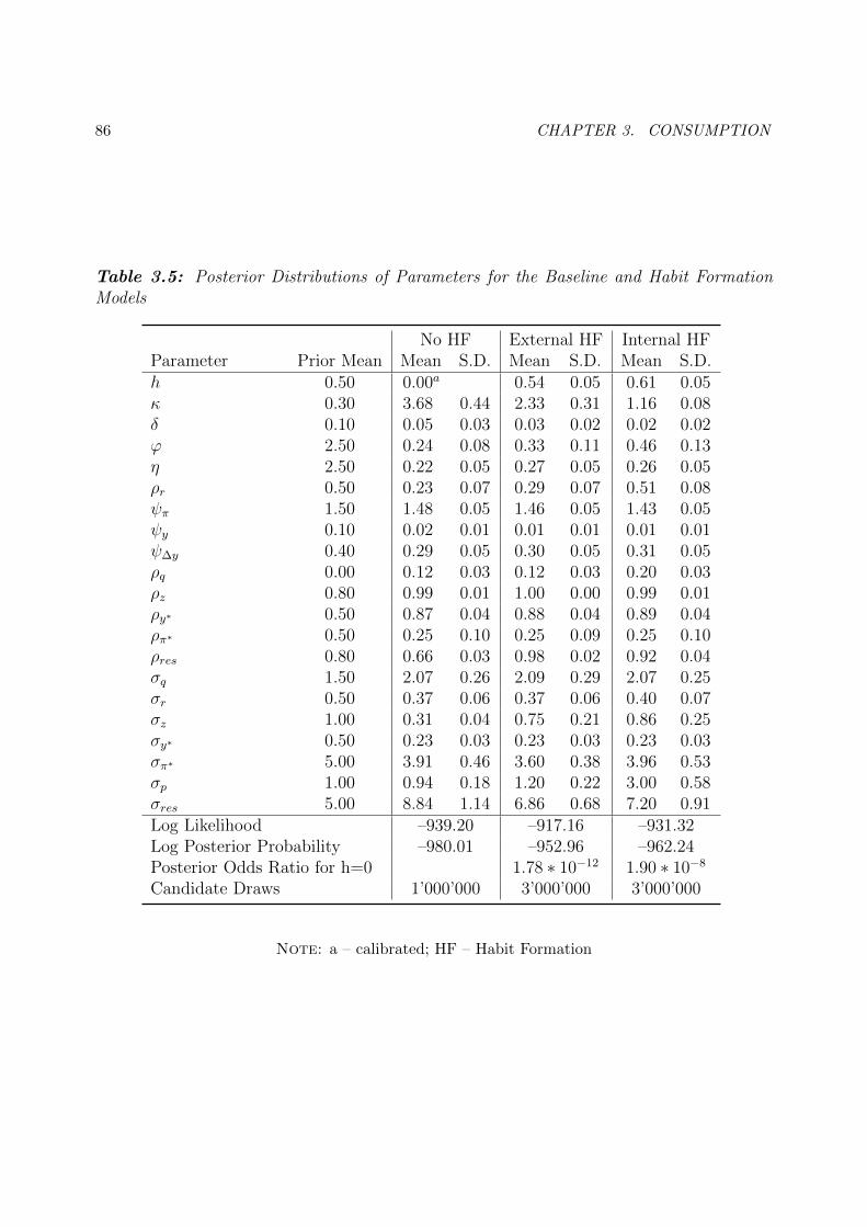
86 CHAPTER 3. CONSUMPTION
Table 3.5: Posterior Distributions of Parameters for the Baseline and Habit FormationModels
No HF External HF Internal HFParameter Prior Mean Mean S.D. Mean S.D. Mean S.D.h 0.50 0.00a 0.54 0.05 0.61 0.05κ 0.30 3.68 0.44 2.33 0.31 1.16 0.08δ 0.10 0.05 0.03 0.03 0.02 0.02 0.02ϕ 2.50 0.24 0.08 0.33 0.11 0.46 0.13η 2.50 0.22 0.05 0.27 0.05 0.26 0.05ρr 0.50 0.23 0.07 0.29 0.07 0.51 0.08ψπ 1.50 1.48 0.05 1.46 0.05 1.43 0.05ψy 0.10 0.02 0.01 0.01 0.01 0.01 0.01ψ∆y 0.40 0.29 0.05 0.30 0.05 0.31 0.05ρq 0.00 0.12 0.03 0.12 0.03 0.20 0.03ρz 0.80 0.99 0.01 1.00 0.00 0.99 0.01ρy∗ 0.50 0.87 0.04 0.88 0.04 0.89 0.04ρπ∗ 0.50 0.25 0.10 0.25 0.09 0.25 0.10ρres 0.80 0.66 0.03 0.98 0.02 0.92 0.04σq 1.50 2.07 0.26 2.09 0.29 2.07 0.25σr 0.50 0.37 0.06 0.37 0.06 0.40 0.07σz 1.00 0.31 0.04 0.75 0.21 0.86 0.25σy∗ 0.50 0.23 0.03 0.23 0.03 0.23 0.03σπ∗ 5.00 3.91 0.46 3.60 0.38 3.96 0.53σp 1.00 0.94 0.18 1.20 0.22 3.00 0.58σres 5.00 8.84 1.14 6.86 0.68 7.20 0.91Log Likelihood –939.20 –917.16 –931.32Log Posterior Probability –980.01 –952.96 –962.24Posterior Odds Ratio for h=0 1.78 ∗ 10−12 1.90 ∗ 10−8
Candidate Draws 1’000’000 3’000’000 3’000’000
Note: a – calibrated; HF – Habit Formation

3.3. HABIT FORMATION 87
Other Model Parameters
The three model versions differ with respect to the Euler equation and the expression for
marginal costs. Accordingly, the estimations produce not only different values for the habit
persistence parameter, but also for the parameter κ. While the mean of κ lies at 3.68 in the
version without habit formation, the versions with habit formation produce smaller values.
In the case of external habit formation, κ comes to lie at 2.33, implying a θ of 0.24. The
version with internal habit formation produces a κ of 1.45, implying a θ of 0.35. The latter
still corresponds to prices being fixed more often than every second quarter on average. The
price stickiness thus turns out smaller than expected in all three model versions. On the
other hand, the degree of indexation to past inflation, δ, lies below 0.1 for all three versions.
Most of the remaining model parameters turn out similar across the model versions.
While, ϕ, the inverse elasticity of labor supply turns out to be higher for the versions with
habit formation, the posterior mean for η, the elasticity of substitution between domestic
and foreign goods, as well as the results for the Taylor rule, are very similar for the three
versions. On the other hand, there are differences for σp, the standard deviation of the
innovations to the preference shock. These differences can be explained by the varying
model structures: the preference shock enters the Euler equation with different coefficients.
Furthermore, the preference shock also enters the Phillips curve in the model with internal
habit formation.
Model Comparison
Statistics on the goodness of fit of the three model versions are given at the bottom of
table 3.5. According to the log likelihood and the log posterior probability, the models
allowing for habit formation are able to fit the data better than the model without habit
formation. This is in line with the habit persistence parameter being significantly above
zero. Furthermore, the posterior odds ratio between the model without habit formation and
those allowing for habit formation can be taken as a criterion for the null hypothesis h = 0.
The posterior odds ratio clearly favors the models allowing for habit formation. Comparing
the log likelihood and log posterior probability of the models with external and internal
habit formation shows that the model with external habit formation reaches a better fit of
the data. Together with the finding that the habit persistence parameter is significantly
different from zero, these results support the concept of habit formation.

88 CHAPTER 3. CONSUMPTION
Impulse Response Functions
Figure 3.3 shows the impulse responses of consumption, output, the interest rate and infla-
tion to shocks to the interest rate and the productivity level for the three model versions.
The impulse response functions show the expected differences between the models: while
the version without habit formation produces immediate reactions, the versions allowing for
habit formation generate delayed reactions. A positive shock to the interest rate causes a
temporary drop in consumption. In the baseline model, consumption reacts strongly in the
first period and comes back to the equilibrium level in the second period already. Conversely,
cosumption initially falls less in the habit formation models and then converges gradually
back to the original level. The effect wears out after about seven quarters. A productivity
shock creates persistent responses of consumption in all three model versions. In contrast
to the reactions to the interest rate shock, the impulse responses to a productivity shock are
hump-shaped. Again, the habit formation models produce more delayed reactions: while
the impulse response reaches its peak in the second quarter in the model without habit
formation, the peak is not reached until the eighth quarters in the habit formation models.
The confidence intervals of the impulse response functions of the habit formation models
are shown in figures 3.7 and 3.8 in the appendix. The confidence interval of the reaction
of consumption to an interest rate shock is generally larger in the habit formation models
than in the baseline model. This is due to the more complex structure of the Euler equation
in these model versions: while the interest rate enters the Euler equation with a factor
of one in the baseline model, the factors are (1 − h) for external habit formation and
(1 − h)(1 − hβ) for internal habit formation. The larger confidence intervals can thus
be explained by the variance of the parameter h. The confidence intervals in the impulse
responses to a productivity shock are generally larger as there are more parameters involved.
For example, the reaction of consumption to a productivity shock depends on ρz (determines
the persistence of the shock), ϕ (determines the effect of productivity on marginal costs),
κ (determines the effect of marginal costs on inflation) and additionally h in the habit
formation models (determines the effect of inflation on consumption).
3.4 Rule-of-Thumb Consumers
This section discusses the role of rule-of-thumb consumers in the small open economy model.
Rule-of-thumb consumers are a special type of consumers which does not face a saving-
spending trade-off. Instead, rule-of-thumb consumers spend all of their labor income on

3.4. RULE-OF-THUMB CONSUMERS 89
Figure 3.3: Comparison of the Impulse Response Functions of the Baseline Model and theHabit Formation Models
Rea
ctio
n of
con
sum
ptio
n
Shock to interest rate
2 4 6 8 10
−1.2
−1.0
−0.8
−0.6
−0.4
−0.2
0.0
Shock to productivity level
0 10 20 30 40 50
0.0
0.2
0.4
0.6
0.8
1.0
1.2
Rea
ctio
n of
out
put
2 4 6 8 10
−0.6
−0.5
−0.4
−0.3
−0.2
−0.1
0.0
0 10 20 30 40 50
0.0
0.1
0.2
0.3
0.4
0.5
Rea
ctio
n of
inte
rest
rat
e
2 4 6 8 10
0.0
0.2
0.4
0.6
0.8
1.0
0 10 20 30 40 50
−0.10
−0.08
−0.06
−0.04
−0.02
0.00
Rea
ctio
n of
infla
tion
2 4 6 8 10
−5
−4
−3
−2
−1
0
0 10 20 30 40 50
−0.12
−0.10
−0.08
−0.06
−0.04
−0.02
0.00
No Habit Formation External Habit Formation Internal Habit Formation
Note: Impulse Responses to a one percent interest rate shock (left) and to a productivity shock(right) of magnitude 1

90 CHAPTER 3. CONSUMPTION
consumption in each time period. As the consumption behaviour of rule-of-thumb house-
holds is determined by the real wage and the amount of hours worked, I estimate the model
under two alternative labor market structures, namely perfectly and imperfectly competi-
tive labor markets. In most small DSGE models, labor markets are assumed to be perfectly
competitive, i.e. individual workers choose the amount of hours they work given the market
wage. The market wage in turn comes to lie at the level at which aggregate labor supply by
workers matches labor demand by firms. When labor markets are assumed to be imperfectly
competitive, some market power is usually given to unions: the latter set wages and workers
then meet firms’ labor demand.
In order to avoid indeterminacy as well as identification problems, I additionally fix
three model parameters when estimating the model variants. The estimated share of rule-
of-thumb consumers among all consumers is significantly different from zero for both labor
market structures. However, allowing for rule-of-thumb behaviour improves the posterior
probability only under perfectly competitive labor markets. Under imperfectly competitive
labor markets, on the other hand, the posterior probability does not change noticeably and
the estimated share of rule-of-thumb consumers is not completely robust to the specification
of the prior distribution.
3.4.1 Motivation
Rule-of-thumb consumers are mainly used in two macreoeonomic contexts. First, they are
introduced in consumption models in order to remedy for some of the discrepancies between
the implications of the PIH and the empirical evidence. Second, they are used in the
literature on fiscal multipliers in order to reproduce the empirical reactions of consumption
to government spending shocks in neoclassical and new Keynesian models.
As in the case of habit formation, discrepancies between the PIH and the data are one
starting point for the modeling of rule-of-thumb consumers. Empirical evidence suggests
that consumption is more strongly correlated with current income than the PIH postulates
(see, e.g. Hall and Mishkin, 1982)4. Campbell and Mankiw (1989) show that this form of
“excess sensitivity” can be explained by a model in which two types of consumers coexist.
Half the consumers operate in line with the PIH and make consumption decisions based on
4This is no contradiction to the arguments made in section 3.3. The motivation for habit formation is thatconsumption reacts slower to changes in income than the PIH suggests. The motivation for rule-of-thumbconsumers is that consumption reacts stronger to changes in current income than the PIH suggests.

3.4. RULE-OF-THUMB CONSUMERS 91
their permanent income. Consumers of this type are also called Ricardian consumers. The
remaining consumers, called rule-of-thumb consumers, simply spend their current income in
each time period and do not save. As a result, the change in consumption can be expressed
as a weighted average of the changes in current and permanent income. While Campbell
and Mankiw (1989) report clear evidence for the existence of rule-of-thumb consumers, they
nevertheless note that not all consumers seem to consume current income: the fact that
periods in which consumption is high relative to income are often followed by rapid income
growth suggests that at least some consumers are forward-looking. Therefore, Campbell
and Mankiw (1989) argue that the optimal model for consumption contains both Ricardian
and rule-of-thumb consumers.
In the context of fiscal multipliers, rule-of-thumb consumers are added to models in order
to reproduce impulse responses as they are found in empirical studies. Impulse response
functions calculated using VAR models usually suggest a positive response of consumption
to expansionary fiscal policy shocks. For US data, impulse responses from identified VAR
approaches are documented for example in Fatas and Mihov (2000) or Blanchard and Perotti
(2002). While this positive response of consumption can well be reproduced in IS-LM
models, where consumption depends on current disposable income, standard neoclassical
models generate a different outcome: as consumers anticipate that an increase government
spending will eventually be financed by an increase in taxes, they view the increase in
spending as a drop in their income. Consequently, they cut consumption and increase labor
supply (see, e.g. Baxter and King, 1993, Galı et al., 2007). The higher labor supply then
leads to a drop in real wages which lowers income and consumption further. Adding rule-
of-thumb consumers can help to reproduce the empirical results if the fiscal shock causes
real labor income to rise. While labor demand will always rise in response to this kind of
shock, the reaction of the real wage can go in either direction. Galı et al. (2007) show that
under sticky prices, the real wage can rise in response to a government spending shock and
generate an increase in labor income. A sufficiently large share of rule-of-thumb consumers
then assures a positive reaction of overall consumption. In line with this result, Forni et al.
(2009) find “mild Keynesian effects” of government spending using an estimated DSGE
model for the Euro Area. However, a rise of the real wage in response to a government
spending shock is doubted for example by Coenen and Straub (2005). Instead, Coenen
and Straub (2005) argue that a positive reaction of consumption to a government spending
shock is unlikely to occur in a DSGE model.

92 CHAPTER 3. CONSUMPTION
The arguments mentioned so far explain why macroeconomists might include rule-of-
thumb consumers in their models. However, in order for this extension to be plausible,
there also needs to be some a priori reason why consumers might not save. One possible
justification is limited asset markets participation (Bilbiie, 2008). Accordingly, rule-of-
thumb consumers do not hold assets and do not smooth consumption because they cannot
access asset markets. Other reasons brought forward are myopia or fear of saving (Galı et al.,
2007). An intuitive reason is mentioned by Mankiw (2000): many households might not have
the financial wherewithal to smooth consumption by saving. Instead, their consumption
moves with current income.
Estimates of the share of rule-of-thumb consumers typically lie between 0.25 and 0.5.
Using time series regressions, Campbell and Mankiw (1989) estimate shares of about 0.5.
In studies using DSGE models for the Euro Area, Forni et al. (2009) estimate shares of
about 0.35, depending on the labor market structure, while Coenen and Straub (2005)
estimate shares of 0.25 to 0.37, depending on the tax system imposed. In their theoretical
analysis of government spending effects, Galı et al. (2007) calibrate the share of rule-of-
thumb consumers at 0.5. For Switzerland, Madsen and McAleer (2001) find a share of 0.18
and Evans and Karras (1998) a share of 0.37, both using time series estimation. To my
knowledge, no estimations from DSGE models are available for Switzerland. In the SNB’s
DSGE model, Cuche-Curti et al. (2009) calibrate the share of rule-of-thumb consumers at
0.7.
3.4.2 Implementation
Extension of the household sector
The model now contains a continuum of households i ∈ [0, 1] which are divided into two
fractions. The first fraction 1− sr of households, called Ricardian or optimizing households,
has access to capital markets and chooses the optimal intertemporal consumption path
with respect to lifetime utility. The second fraction sr of households, called rule-of-thumb
households, spends all its labor income on consumption in each period. Variables referring
to optimizing consumers are denoted by an “o” superscript, variables referring to rule-of-
thumb consumers by an “r” superscript. Both consumer types have the familiar utility
function:
E0
∞∑t=0
βtεp,t
(log(Cit − hCi
t−1
)− (N i
t )1+ϕ
1 + ϕ
), for i = {o, r}

3.4. RULE-OF-THUMB CONSUMERS 93
According to the results from the previous section, I impose external habit formation in
the model variant with perfectly competitive labor markets – the variant with imperfectly
competitive labor markets cannot be estimated under habit formation due to indeterminacy
problems. Furthermore, I assume the preference shock to be equal for the two consumer
types. Ricardian consumers face the familiar budget constraint from the baseline model:
PtCot +
1
Rt
Dot+1 +
εtR∗tD∗,ot+1 = WtPtN
ot +Do
t + εtD∗,ot + Πo
t
I assume the real wage to be equal for both consumer types. Rule-of-thumb consumers face
a reduced budget constraint:
PtCrt = WtPtN
rt
As a result, their consumption level is equal to their real labor income:
Crt = WtN
rt
Consumption and hours worked can be aggregated using the share of rule-of-thumb con-
sumers, sr:
Ct = srCrt + (1− sr)Co
t
Nt = srNrt + (1− sr)N o
t
Labor Market Structures
I consider perfectly competitive labor markets and imperfectly competitive labor markets.
Under perfectly competitive labor markets, individual workers choose the amount of hours
they work given the market wage. The market wage in turn comes to lie at the level at
which aggregate labor supply by workers matches labor demand by firms. Under imper-
fectly competitive labor markets, wages are set by unions and workers then meet firms’ labor
demand. In both cases, the wage level is equal for rule-of-thumb and Ricardian workers.
Moreover, an identical relation between the wage level, aggregate hours worked and aggre-
gate consumption holds under both structures. However, while the amount of hours worked
by the two household types is allowed to differ under perfectly competitive labor markets,
both types work the same amount of hours under imperfectly competitive labor markets.
Under perfectly competitive labor markets, both consumer types face an analog in-
tratemporal optimality condition. This condition determines for both consumer types the

94 CHAPTER 3. CONSUMPTION
relation between hours worked and the marginal utility of consumption, given the real wage:
(N it
)ϕ (Cit − hCi
t−1
)= Wt, for i = {o, r}
This corresponds to the labor market structure I assumed in section 3.3. Although the
wage level is equal for both consumer types, hours worked and consumption will generally
differ.
In the model variant with imperfectly competitive labor markets, I follow Galı et al.
(2007) and assume a continuum of differentiated labor/worker types j ∈ [0, 1]. Effective
labor hired by firm k is now an aggregate of the different labor types:
Nt(k) =
(∫ 1
0
Nt(j, k)εw−1εw dj
) εwεw−1
(3.28)
where εw denotes the elasticity of substitution between the labor types. Each worker type
is represented by a specific union. The fraction of Ricardian and rule-of-thumb households
is uniformly distributed across the worker types and unions. In hiring labor, firms do not
discriminate between Ricardian and rule-of-thumb households. A typical union sets the
wage for its worker type z in each period according to the objective function
sr
[(Crt (z)− hCr
t−1(z))Wt(z)Nt(z)− Nt(z)1+ϕ
1 + ϕ
]+ (1− sr)
[(C0t (z)− hC0
t−1(z))Wt(z)Nt(z)− Nt(z)1+ϕ
1 + ϕ
]and subject to the labor demand by firms
Nt(z) =
(Wt(z)
Wt
)−εwNt
The labor demand function can be derived from equation (3.28) by assuming cost minimiza-
tion by firms; details are given in the appendix. In principle, the unions maximize real labor
income minus disutility of labor for their worker types. However, as the consumption level
will generally differ between Ricardian and rule-of-thumb households, unions weight labor
income with the respective marginal utility of consumption. Furthermore, unions take into
account that firms do not discriminate between Ricardian and rule-of-thumb households.
This implies that in the aggregate, hours worked will be equal for the household types, i.e.

3.4. RULE-OF-THUMB CONSUMERS 95
N rt = N0
t = Nt. As the labor types and unions are assumed to be symmetric, the index
z can be dropped. The first order condition to the unions’ maximization problem is then
given by (sr
MRSrt+
1− srMRS0
t
)Wt =
εwεw − 1
where MRSit = (Cit − hCi
t−1)Nϕt for i = {o, r}.
Changes in the Linearized Model
I assume for simplicity that the steady state consumption levels of both consumer types
are equal, i.e. Co = Cr = C. While there are arguments against this assumption, equal
steady-state consumption could always be obtained by modeling a government sector which
makes transfers to the consumer types in a suitable way (Galı et al., 2007). Steady state
hours worked are then also equalized: under perfectly competitive labor markets, an analog
intratemporal optimality condition holds for both consumer types and equal steady state
consumption thus implies equal steady state hours worked. Under imperfectly competitive
labor markets, the amount of hours worked is always equal for the two consumer types.
Consumption and hours worked can then be aggregated as follows:
ct = srcrt + (1− sr) cot (3.29)
nt = srnrt + (1− sr)not (3.30)
For Ricardian consumers, the standard Euler equation determines the consumption
path: (cot − hcot−1
)= Et
[cot+1 − hcot
]− (1− h) (rt − Et [πt+1])
+ (1− h)Et [εp,t − εp,t+1](3.31)
For rule-of-thumb consumers, consumption equals labor income:
crt = wt + nrt
The linearized intratemporal optimality condition for perfectly competitive labor markets
is given by
ϕnit = wt −1
(1− h)
(cit − hcit−1
), for i = {o, r} (3.32)

96 CHAPTER 3. CONSUMPTION
For the case of imperfectly competitive labor markets, the linearized first order condition
to the unions’ maximization problem is given by
wt = ϕnt +1
(1− h)(ct − hct−1) (3.33)
Note that this condition also holds under perfectly competitive labor markets and can
be constructed by combining equations (3.29), (3.30) and (3.32). The two labor market
structures therefore result in an identical relation between the real wage and aggregate
consumption as well as aggregate hours worked. However, hours worked are allowed to
differ between Ricardian and rule-of-thumb consumers under perfectly competitive labor
markets.
As the real wage is a key variable for the behaviour of rule-of-thumb consumers, it is
worth to shortly highlight its determinants. Equation (3.33) states that the real wage is
equal to the marginal rate of substitution between consumption and leisure. If the amount
of hours worked rises, marginal utility of leisure rises and workers (or unions) ask for higher
wages. The size of this effect depends on the elasticity of labor supply and therefore on the
parameter ϕ: a low (high) elasticity of labor supply, corresonding to a high (low) parameter
ϕ, leads to strong (weak) reaction of the real wage. Furthermore, a higher consumption level
and/or consumption growth lowers marginal utility of consumption and thus also causes
workers (unions) to ask for higher wages. Under habit formation, the size of this effect
increases with the habit persistence parameter h. Summarizing the implications of equation
(3.33), we note that whenever nt and ct move into the same direction, wt also moves into
this direction. On the other hand, if nt and ct move into opposite directions, the reaction
of wt depends on the parameters ϕ and h.
3.4.3 Effects on Determinacy
This section discusses the effect of the introduction of rule-of-thumb consumers on the
determinacy of the model solution. A frequent source of indeterminacy in macroeconomic
models is a weak reaction of the monetary authority to inflation (this corresponds to the
parameter ψπ being too small). Woodford (2001) shows that for a Taylor rule where the
central bank reacts to inflation and the output cycle, the condition for a unique equilibrium
in a standard new Keynesian model (i.e., without rule-of-thumb consumers) is given by
ψπ > 1− (1− β)ψyκ (1 + ϕ)
(3.34)

3.4. RULE-OF-THUMB CONSUMERS 97
This condition is also called the “Taylor principle”5. Accordingly, the required reaction
to inflation is lower if the central bank also reacts to output (i.e., ψy > 0). Moreover, a
higher degree of price stickiness (corresponding to a lower κ) and/or a lower elasticity of
labor supply (corresponding to a higher ϕ) lower the threshold value for ψπ. If the central
bank does not react to output, the condition reduces to ψπ > 1. It is often argued that the
fluctuations in output and inflation in the US in the 1960s and 1970s may have been caused
by the Federal Reserve responding too little to inflation (see, e.g. Galı et al., 2004).
The presence of rule-of-thumb consumers alters the condition for determinacy. Galı
et al. (2004) show that if the share of rule-of-thumb consumers is large enough, the Taylor
principle can be an insufficient condition to guarantee determinacy. Instead, a high degree
of price stickiness can lead to indeterminacy even if the Taylor principle holds. In order
to give intuition on this result, Galı et al. (2004) consider an increase in economic activity
which is not caused by fundamental shocks and which agents expect to wear out only
gradually. As a consequence, inflation would increase and the central bank would raise
the interest rate. Without the existence of rule-of-thumb consumers, such a boom would
not be a rational expectations equilibrium because the higher interest rate would cause
consumption to decrease and economic activity to decline. However, the presence of rule-
of-thumb consumers can change this mechanism: depending on the model parameters, the
higher labor demand by firms, together with sticky prices, could raise the real wage level.
Rule-of-thumb consumers would then increase their consumption spending and depending
on their share, their demand could sustain the boom. In this case, the central bank would
not be able to control economic activtiy. Thus, any arbitrary change (i.e., a change not
caused by fundamental shocks) in expectations could alter the equilibrium of the economy.
Mathematically, the possibility of multiple equilibria leads to indeterminate model solutions.
Depending on the structure of the model, there is thus a threshold share of rule-of-
thumb consumers above which model solutions are indeterminate. In addition to the degree
of price stickiness, there are several other factors which affect this threshold share. As the
key mechanism leading to indeterminacy is the direct reaction of rule-of-thumb consumers
to changes in the real wage, any factor which affects the dynamics of the real wage also
affects determinacy properties. Galı et al. (2004) discuss the role of the elasticity of labor
supply in this context. In the case of an unexpected boom as discussed above, a lower
5This condition cannot directly be applied to the setting in the present paper as in the Taylor rule usedhere, the central bank is allowed to react to output growth.

98 CHAPTER 3. CONSUMPTION
elasticity of labor supply requires a stronger increase in the real wage in order for labor
supply to meet the higher labor demand. But a stronger reaction of the real wage leads to
a stronger reaction in rule-of-thumb consumers’ spending, which in turn reduces the ability
of the central bank to control consumption demand. Therefore, a lower elasticity of labor
supply (i.e., a higher parameter ϕ) lowers the threshold share of rule-of-thumb consumers
above which indeterminacy occurs. Bilbiie (2008) examines the interaction of labor and
assets markets and finds that a low elasticity of labor supply, together with a sufficiently
large share of rule-of-thumb consumers, can actually change the sign of the IS curve (i.e.,
the relation between the interest rate and output). In this case, an inverted Taylor principle
holds: determinacy requires the monetary authority to lower the interest rate in response to
inflation. The model used in Bilbiie (2008) captures the effects of hours worked and wages
on profits as well as the flow of profits to Ricardian consumers.
General assumptions on the labor market structure also affect determinacy proper-
ties. Simulations in Motta and Tirelli (2010) show that indeterminacy problems increase if
imperfectly competitive labor markets are assumed instead of perfectly competitive labor
markets. The critical share of rule-of-thumb consumers above which model solutions are
indeterminate is thus smaller under imperfectly competitive labor markets. Although the
model structure in Motta and Tirelli (2010) is slightly different than mine, I found this
finding confirmed in the estimation process. A possible explanation for this higher tendency
to indeterminacy is the labor supply of the consumer types. Under perfectly competitive
labor markets, both consumer types choose their amount of hours worked individually ac-
cording to the market wage and to their marginal utility of consumption. In the scenario
of an unexpected boom discussed above, Ricardian consumers cut their consumption level
while rule-of-thumb consumers extend their consumption level. As these reactions affect the
respective marginal utilities of consumption, Ricardian consumers will work more and rule-
of-thumb consumers will work less. This dampens the increase in rule-of-thumb consumers’
labor income and therefore the problematic positive response of rule-of-thumb consumers
to the rise in the real wage. However, this effect vanishes once hours worked are equalized
in the imperfectly competitive case: now, the difference in hours worked will lie between
the optimal reaction for Ricardian and rule-of-thumb consumers and the positive reaction
of rule-of-thumb consumers to the increase in the real wage turns out even stronger.
Finally, the effect of habit formation on determinacy is noteworthy. As the impulse re-
sponse functions in section 3.3 show, habit formation leads to sluggish reactions of Ricardian
consumers to monetary policy shocks. Habit formation thus undermines the effectiveness of

3.4. RULE-OF-THUMB CONSUMERS 99
monetary policy in general and lowers the critical share of rule-of-thumb consumers above
which indeterminacy occurs. Indeed, allowing for habit formation created substantial inde-
terminacy problems under imperfectly competitive labor markets in my estimations.
Introducing rule-of-thumb consumers can thus create various problems with indeter-
minacy. In the algorithm used in this paper, indeterminacy leads to bounded parameter
spaces: as all parameter sets implying indeterminate model solutions are rejected, the share
of rule-of-thumb consumers is restricted below its critical value. In order to avoid such
boundaries to affect the estimation results, I fix ϕ, the inverse of the elasticity of labor
supply, at a low value. Furthermore, stronger indeterminacy problems require estimating
the model variant with imperfectly competitive labor markets without habit formation.
3.4.4 Priors
The prior distributions for this section’s estimations are shown in table 3.6. They are
identical to those from section 3.3 with the exception of the parameters ϕ, η, ψy and sr. ϕ
is fixed at 0.1 in order to avoid indeterminacy problems due to combinations of low labor
supply elasticites and high shares of rule-of-thumb consumers. I chose a value below the
esimation results from sections 3.2 and 3.3 in order to rule out indeterminacy problems as
far as possible. Apart from indeterminacy problems, the estimation of the model variants
with rule-of-thumb consumers was subject to identification problems and slow convergence
in general. In order to avoid these problems, I fix the parameters η and ψy. The parameter
η, which measures the elasticity of substitution between domestic and foreign goods, was
itself subject to identification problems and diverged to zero in some model specifications.
According to the estimation results from section 3.3, I therefore fix η at 0.25. The parameter
ψy, which measures the response of the central bank to the output cycle, was estimated
to be approximately zero in the previous sections. With this parameter fixed at zero,
the remaining parameter estimates converged faster. Furthermore, the habit persistence
parameter h is restricted to 0 for the model version with imperfectly competitive labor
markets. For the share of rule-of-thumb consumers (sr), I set a relatively neutral normal
distribution with a mean of 0.5 and standard deviation of 0.25.
3.4.5 Results
The posterior means are shown in table 3.7. Under perfectly competitive labor markets,
the estimates converged after generating 5’750’000 candidate draws when the share of rule-

100 CHAPTER 3. CONSUMPTION
Table 3.6: Prior Distributions of Parameters for the Models with Rule-of-Thumb Con-sumers
Parameter Distribution Mean Standard Deviationsr Normal on [0,1] 0.50 0.25h Beta 0.50 0.20β calibrated 0.99α calibrated 0.27κ Gamma 0.30 0.30δ Normal on [0,1] 0.10 0.05ϕ calibrated 0.10η calibrated 0.25ρr Beta 0.50 0.20ψπ Gamma 1.50 0.05ψy calibrated 0.00ψ∆y Normal > 0 0.40 0.05ρq Normal 0.00 0.50ρz Normal 0.80 0.50ρy∗ Normal 0.50 0.50ρπ∗ Normal 0.50 0.50ρp calibrated 0.90ρi Normal 0.80 0.50C/Y calibrated 0.60C∗H calibrated 0.40σq Inv.Gamma 1.50 1.50σr Inv.Gamma 0.50 0.50σz Inv.Gamma 1.00 1.00σy∗ Inv.Gamma 0.50 0.50σπ∗ Inv.Gamma 5.00 3.50σp Inv.Gamma 1.00 3.50σres Inv.Gamma 5.00 3.50

3.4. RULE-OF-THUMB CONSUMERS 101
of-thumb consumers was restricted to zero. For the unrestricted version, the estimates
converged after generating 4’000’000 candidate draws. Under imperfectly competitive labor
markets, the estimates converged after generating 2’000’000 candidate draws for both the
restricted and unrestricted version.
Share of Rule-of-Thumb Consumers
The share of rule-of-thumb consumers is estimated at 0.65 under perfectly competitive
labor markets and at 0.53 under imperfectly competitive labor markets. The assumed labor
market structure thus affects the estimates. However, the rather large standard deviation
under perfectly competitive labor markets indicates that the parameter is not estimated with
a high precision. On the other hand, the precision seems to be higher under imperfectly
competitive labor markets. The posterior plots are shown in figure 3.4 and reveal that
the parameter’s posterior distribution is skewed to the left under perfectly competitive
labor markets; the mode lies above the mean at approximately 0.75. Under imperfectly
competitive labor markets, mode and mean lie close to each other. In both cases, the
share of rule-of-thumb consumers is significantly different from zero. In order to check the
dependence of these results on the specification of the prior mean, I run the estimations also
with prior means of 0.25 and 0.70 for sr. A prior mean of 0.75 was not possible for the model
variant with imperfectly competitive labor markets as it resulted in an indeterminate model
solution at the prior means of the parameters and the algorithm was therefore not able
to initialize. Under perfectly competitive labor markets, sr converges to 0.56 (prior mean
0.25) and 0.69 (prior mean 0.70). Under imperfectly competitive labor markets, sr converges
to 0.23 (prior mean 0.25) and 0.50 (prior mean 0.70). For both labor market structures,
the lower prior mean of 0.25 alters the posterior mean. While the order of magnitude
of the posterior mean stays the same for perfectly competitive labor markets, it changes
considerably for imperfectly competitive labor markets. On the other hand, the higher prior
mean of 0.70 leads to almost identical results for both labor market structures. Summarizing,
the parameter estimation results support the concept of rule-of-thumb consumers under both
perfectly and imperfectly competitive labor markets. However, the estimated share of rule-
of-thumb consumers is not robust to the specification of the prior mean under imperfectly
competitive labor markets.

102 CHAPTER 3. CONSUMPTION
Table 3.7: Posterior Distributions of Parameters for the Models with Rule-of-Thumb Con-sumers
Perfectly Competitive LM Imperfectly Competitive LMWithout ROT With ROT Without ROT With ROT
Prior Mean Mean S.D. Mean S.D. Mean S.D. Mean S.D.sr 0.50 0.00a 0.65 0.12 0.00a 0.53 0.04h 0.50 0.56 0.05 0.61 0.06 0.00a 0.00a
κ 0.30 2.04 0.22 3.38 0.56 4.51 0.80 2.50 0.23δ 0.10 0.04 0.03 0.07 0.04 0.06 0.04 0.05 0.03ρr 0.50 0.36 0.07 0.27 0.08 0.25 0.07 0.25 0.07ψπ 1.50 1.45 0.05 1.48 0.05 1.48 0.05 1.49 0.05ψ∆y 0.40 0.31 0.05 0.30 0.05 0.32 0.05 0.32 0.05ρq 0.00 0.17 0.03 0.13 0.03 0.11 0.03 0.09 0.03ρz 0.80 0.99 0.01 0.99 0.01 0.99 0.01 1.00 0.00ρy∗ 0.50 0.89 0.04 0.87 0.04 0.88 0.04 0.89 0.03ρπ∗ 0.50 0.25 0.10 0.25 0.10 0.25 0.10 0.25 0.10ρres 0.80 0.82 0.05 0.87 0.05 0.82 0.05 0.96 0.02σq 1.50 2.09 0.27 2.06 0.27 2.07 0.27 2.06 0.26σr 0.50 0.38 0.06 0.38 0.06 0.38 0.06 0.39 0.06σz 1.00 1.04 0.26 1.32 0.45 0.33 0.04 0.38 0.05σy∗ 0.50 0.23 0.03 0.23 0.03 0.23 0.03 0.23 0.03σπ∗ 5.00 3.96 0.53 3.95 0.55 3.97 0.51 3.94 0.52σp 1.00 1.64 0.31 1.06 0.25 1.04 0.24 0.92 0.18σres 5.00 6.46 0.84 6.54 0.90 6.65 0.89 6.89 0.87Log Likelihood –915.51 –901.74 –925.64 –932.15Log Posterior Probability –934.11 –924.17 –951.59 –950.87Posterior Odds Ratiofor sr = 0 4.84 ∗ 10−5 4.87 ∗ 10−1
Candidate Draws 5’750’000 4’000’000 2’000’000 2’000’000
Note: a – calibrated; ROT – rule-of-thumb consumers; LM – labor markets

3.4. RULE-OF-THUMB CONSUMERS 103
Figure 3.4: Posterior Plots for the Share of Rule-of-Thumb Consumers
Perfectly Competitive Labor Markets
0.0 0.2 0.4 0.6 0.8 1.0
0
1
2
3
4
Imperfectly Competitive Labor Markets
0.0 0.2 0.4 0.6 0.8 1.0
0
2
4
6
8
Prior Distribution Posterior Distribution Posterior Mean

104 CHAPTER 3. CONSUMPTION
Other Model Parameters
With regard the other model parameters, mainly the parameter κ shows differences between
the model versions. These differences can be explained by the differing intratemporal opti-
mality conditions and structures of marginal costs. The implicitly estimated price stickiness
parameters θ range between 0.15 (imperfectly competitive labor markets without rule-of-
thumb consumers) and 0.26 (perfectly competitive labor markets without rule-of-thumb
consumers). In all model versions, the estimation results imply prices to be fixed more often
than every second quarter.
The remaining model parameters turn out very similarly across the model versions.
Minor differences are visible in the autoregressive parameters of the Taylor rule and of
the exogenous process for the terms of trade as well as in the standard deviation of the
innovations to the preference shock.
Model Comparison
Statistics on the goodness of fit of the model variants are given at the bottom of table 3.7.
Under perfectly competitive labor markets, the model variant allowing for rule-of-thumb
consumers reaches a better likelihood as well as a better posterior probability than the
variant without rule-of-thumb consumers. Under imperfectly competitive labor markets,
however, the restricted version reaches a better log likelihood. The posterior probability
is almost identical, indicating bigger deviations between prior distributions and posterior
means in the restricted version. Consequently, the posterior odds ratio, which can be taken
as a criterion for the null hypothesis sr = 0, clearly supports the existence of rule-of-
thumb consumers under perfectly competitive labor markets. Under imperfectly competitive
labor markets, the posterior odds ratio marginally favors the version without rule-of-thumb
consumers. Comparing the performance of the two labor market structures, the statistics
indicate that perfectly competitive labor markets are a more appropriate assumption for
Switzerland than imperfectly competitive labor markets.
Impulse Response Functions
Plots showing the impulse response functions for the model versions with rule-of-thumb
consumers are shown in figure 3.5 for perfectly competitive labor markets and in figure 3.6 for
imperfectly competitive labor markets. The plots show the reactions of total consumption,
output, the interest rate and inflation to shocks to the interest rate and to the technology

3.4. RULE-OF-THUMB CONSUMERS 105
level. Furthermore, the effects of a shock to the GDP residual are discussed in the text
below. The reactions of the model are in principle similar under the two labor market
structures. However, the model with imperfectly competitive labor markets produces more
sudden reactions because it does not allow for habit formation.
A positive shock to the interest rate lowers consumption of Ricardian consumers and
therefore output. The lower overall consumption level and the declining labor demand cause
real wages to fall. As a consequence, rule-of-thumb consumers cut their consumption level
as well. Both consumer types thus respond to monetary policy. However, it is important to
note that the reaction of rule-of-thumb consumers is triggered by the reaction of Ricardian
consumers.
A positive shock to the technology level lowers marginal costs as well as labor demand
by firms. As a consequence, inflation decreases and the central bank lowers the interest
rate. These primary effects cause Ricardian consumers to increase their consumption level.
In spite of the corresponding increase in output, the net effect on labor demand is negative.
The real wage is subject to two forces in this setting: while the falling labor demand pushes
wages down, the higher consumption level of Ricardian consumers pushes them up. As the
former effect is very small due to the high elasticity of labor supply, the overall effect on
the real wage is positive. The rise in the real wages is stronger than the reduction in hours
worked and consumption of rule-of-thumb consumers thus increases. Therefore, a positive
technology shock causes an increase in total consumption and output as well as a small
decrease in inflation and the interest rate.
As mentioned, rule-of-thumb consumers are frequently used in order to assess the effects
of government spending shocks on consumption. In my model, such a shock corresponds
to a shock to the GDP residual. As there is no government sector which eventually raises
taxes in order to finance the higher expenses, the full effects of a government spending
shock cannot be analyzed. However, the effect on total consumption turns out negative
even without accounting for the tax effect. The mechanism is as follows. A shock to the
GDP residual directly increases output and labor demand. The central bank then raises
the interest rate and Ricardian consumers cut their consumption level. Taken together,
these effects lower the real wage: due to the high elasticity of labor supply, the higher labor
demand has virtually no effect, but the lower consumption level pulls the wage downwards.
As a consequence, rule-of-thumb consumers cut their consumption level as well and total
consumption falls in response to the government spending shock.

106 CHAPTER 3. CONSUMPTION
Figure 3.5: Impulse Reponses for the Model with Rule-of-Thumb Consumers under Per-fectly Competitive Labor Markets
Rea
ctio
n of
tota
l con
sum
ptio
n
Shock to interest rate
2 4 6 8 10
−0.6
−0.5
−0.4
−0.3
−0.2
−0.1
0.0
Shock to productivity level
0 10 20 30 40 50
0.0
0.2
0.4
0.6
0.8
1.0
1.2
Rea
ctio
n of
out
put
2 4 6 8 10
−0.35
−0.30
−0.25
−0.20
−0.15
−0.10
−0.05
0.00
0 10 20 30 40 50
0.0
0.1
0.2
0.3
0.4
0.5
Rea
ctio
n of
inte
rest
rat
e
2 4 6 8 10
0.0
0.2
0.4
0.6
0.8
1.0
0 10 20 30 40 50
−0.04
−0.03
−0.02
−0.01
0.00
0.01
Rea
ctio
n of
infla
tion
2 4 6 8 10
−8
−6
−4
−2
0
0 10 20 30 40 50
−0.08
−0.06
−0.04
−0.02
0.00
Note: Impulse Responses to a one percent interest rate shock (left) and to a productivity shock(right) of magnitude 1 with 95-percent confidence intervals

3.4. RULE-OF-THUMB CONSUMERS 107
Figure 3.6: Impulse Reponses for the Model with Rule-of-Thumb Consumers under Im-perfectly Competitive Labor Markets
Rea
ctio
n of
tota
l con
sum
ptio
n
Shock to interest rate
2 4 6 8 10
−8
−6
−4
−2
0
Shock to productivity level
0 10 20 30 40 50
0.0
0.2
0.4
0.6
0.8
1.0
Rea
ctio
n of
out
put
2 4 6 8 10
−3
−2
−1
0
0 10 20 30 40 50
0.0
0.1
0.2
0.3
0.4
0.5
Rea
ctio
n of
inte
rest
rat
e
2 4 6 8 10
0.0
0.2
0.4
0.6
0.8
1.0
0 10 20 30 40 50
−0.05
−0.04
−0.03
−0.02
−0.01
0.00
0.01
Rea
ctio
n of
infla
tion
2 4 6 8 10
−20
−15
−10
−5
0
0 10 20 30 40 50
−0.14
−0.12
−0.10
−0.08
−0.06
−0.04
−0.02
0.00
Note: Impulse Responses to a one percent interest rate shock (left) and to a productivity shock(right) of magnitude 1 with 95-percent confidence intervals
108 CHAPTER 3. CONSUMPTION
3.5 Conclusions
This paper analyzes habit formation and rule-of-thumb consumers in a small open economy
model. The model is a simplified version of the model used in Galı and Monacelli (2005).
Using a Markov Chain Monte Carlo method on Swiss data, I estimate the degree of habit
persistence under external and internal habit formation as well as the share of rule-of-thumb
consumers under two labor market structures. Furthermore, I compare the performance of
the model versions.
I find habit persistence parameters of 0.54 in the case of external habit formation and
0.61 in the case of internal habit formation. Both are significantly different from zero.
Allowing for habit formation improves the likelihood as well as the posterior probability of
the model. The direct comparison of the two habit formation models shows that external
habit formation reaches a better posterior probability. With respect to the share of rule-of-
thumb consumers, I find a value of 0.65 under perfectly competitive labor markets and a
value of 0.53 under imperfectly competitive labor markets. Although both estimates are
significantly different from zero, the overall performance of the model does not improve in
both cases. For the variant with perfectly competitive labor markets, the likelihood and
posterior probability improve when rule-of-thumb behaviour is allowed for. For the variant
with imperfectly competitive labor markets, the results are less clear-cut: the parameter
estimates are not perfectly robust and the posterior probability does not allow for a clear
acceptance or rejection of rule-of-thumb consumers.
In future research, the robustness of the results could be checked in more complex
models. For example, the law of one price could be relaxed or investment could be mod-
eled structurally. In the case of rule-of-thumb consumers, additional insights on modeling
features which reduce indeterminacy problems would be useful.

3.A. APPENDIX 109
3.A Appendix
3.A.1 Derivations of Model Equations
Aggregation of Consumption Goods
The perfectly competitive retail sector which buys CH,t and CF,t and sells the aggregated
consumption good Ct to consumers faces the following problem:
maxCH,t,CF,t
PtCt − PH,tCH,t − PF,tCF,t
subject to Ct =
[(1− α)
1ηC
η−1η
H,t + α1ηC
η−1η
F,t
] ηη−1
inserting and taking first order conditions with regard to CH,t and CF,t yields the following
demand functions:
CH,t = (1− α)
(PH,tPt
)−ηCt
CF,t = α
(PF,tPt
)−ηCt
The overall price index Pt can be calculated from a zero profit condition for the retail sector:
0 = PtCt − PH,t(1− α)
(PH,tPt
)−ηCt − PF,tα
(PF,tPt
)−ηCt
Pt =[(1− α)P 1−η
H,t + αP 1−ηF,t
] 11−η
The underlying layer of retailers buys intermediate goods YC,t(i) and aggregates them
to units of the domestic good. This retail sector faces the following problem:
maxYt(i)
PH,tYC,t −∫ 1
0
PH,t(i)YC,t(i)di
subject to YC,t =
[∫ 1
0
YC,t(i)ε−1ε di
] εε−1

110 CHAPTER 3. CONSUMPTION
Inserting and taking first order conditions with respect to Yt(i) yields the demand functions
YC,t(i) =
(PH,t(i)
PH,t
)−εYC,t
The domestic price index PH,t can be calculated from a zero profit condition for this retail
sector:
0 = PH,tYC,t −∫ 1
0
PH,t(i)
(PH,t(i)
PH,t
)−εYC,tdi
PH,t =
[∫ 1
0
PH,t(i)1−εdi
] 11−ε
Imperfectly Competitive Labor Markets: Labor Demand
In order to derive labor demand by firms, an additional sector is assumed in analogy to the
two retail sectors in the section above (see, e.g., Fernandez-Villaverde, 2009). This sector
hires the differentiated labor types, aggregates them to homogenous labor units and sells
these units to the firms of the production sector. The aggregation of homogenous labor
units follows a production function:
Nt(k) =
(∫ 1
0
Nt(z, k)εw−1εw dz
) εwεw−1
where Nt(k) is the labor input sold to firm k, Nt(z, k) is the used amount of hours worked by
labor type z and εw is the elasiticty of substitution among the labor types. The aggregation
sector maximizes profits, taking individual wages Wt(z)Pt and the aggregate wage level WtPt
as given:
maxNt(z)
WtPtNt(k)−∫ 1
0
Wt(z)PtNt(z, k)dz
subject to Nt(k) =
(∫ 1
0
Nt(z, k)εw−1εw dz
) εwεw−1
Inserting and taking first order conditions with respect to Nt(z, k) yields the demand func-
tions
Nt(z, k) =
(Wt(z)
Wt
)−εwNt(k)

3.A. APPENDIX 111
Furthermore, the overall wage index Wt can be aggregated from the individual wages by
assuming zero profits for the aggregation sector:
Wt =
(∫ 1
0
Wt(z)1−εwdz
) 11−εw
Log-Linearization
Prior to the linearization of the model equations, some steady states have to be derived.
Following Del Negro and Schorfheide (2008), I set the steady state of the real exchange rate
to one, i.e. S = 1. From equation (3.11), it then follows that the staedy state of the terms
of trade is also equal to one, i.e. Q = 1. With regard to prices, equation (3.10) states that
PH = P . Together with the price index (3.2), this leads to PF = PH = P . From equation
(3.9), it also follows that C∗H = α∗C∗. Furthermore, I use the approximation c∗t = y∗t .
Euler equation: the linearization of the various versions of the Euler equation is
straightforward.
Real exchange rate: equation (3.11) linearizes to
st = − (1− α) qt (3.35)
Aggregate production function: as mentioned, I assume that the residual Yres,t is
produced according to an individual production function analog to equation (3.5). The
amount of hours worked can then be aggregated by integrating over the firms of both the
production sector of the intermediate consumption good as wall as the implicit production
sector of the residual.
Nt =
∫ 1
0
Nt(i)di =
∫ 1
0
Yt(i)
Ztdi =
YtAtZt
where At =∫ 1
0(Yt(i)/Yt)di. Under perfectly competitive labor markets, Nt(i) corresponds
to the amount of hours worked which labor i hires. Under imperfectly competitive labor
markets on the other hand, Nt(i) corresponds to units of the homogenous labor unit which
firm i hires. Galı and Monacelli (2005) show that variations in log(At) around its steady
state are of second order. Therefore, the following linearized relationship between aggregate
vairables holds up to a first order approximation:
nt = yt − zt (3.36)

112 CHAPTER 3. CONSUMPTION
Phillips curve: the derivation of the Phillips curve involves several steps. In equation
(3.7), the stochastic discount factor Qt+τ |t can be substituted by λt+τ/λt. λt can then be
canceled and the first order condition becomes
Et
[∞∑τ=0
θτλt+τYC,t+τ |t
((PH,t+τ−1
PH,t−1
)δP ′H,t −
ε
ε− 1PH,t+τMCt+τ
)]= 0
By taking the steady state version of this equation, it follows that MC = (ε− 1)/ε. Prior
to linearization, the expression is rearranged to
Et
[∞∑τ=0
θτλt+τYC,t+τ |t
(PH,t+τ−1
PH,t−1
)δP ′H,t
]= Et
[∞∑τ=0
θτλt+τYC,t+τ |tε
ε− 1PH,t+τMCt+τ
]
With respect to the steady states of the left and right hand sides of the above equation, note
that the steady state of λt+τ cancels out only up to βτ , independently of the type of habit
formation imposed in the utility function. Moreover, MC(ε/(ε − 1)) = 1. Linearization
then yields
Et
[∞∑τ=0
(βθ)τ(δ (pH,t+τ−1 − pH,t−1) + p′H,t
)]= Et
[∞∑τ=0
(βθ)τ (pH,t+τ +mct+τ )
]
Rearranging yields
Et
[∞∑τ=0
(βθ)τ(p′H,t − pH,t−1
)]= Et
[∞∑τ=0
(βθ)τ ((δ − 1)pH,t−1 − δpH,t+τ−1 + pH,t+τ +mct+τ )
]1
1− βθ(p′H,t − pH,t−1
)= Et
[∞∑τ=0
(βθ)τ (mct+τ + δπH,t+τ + (δ − 1) (pH,t−1 − pH,t+τ ))
]
p′H,t − pH,t−1 = (1− βθ)Et
[∞∑τ=0
(βθ)τ (mct+τ + δπH,t+τ )
]
+ (1− βθ) (1− δ)Et
[∞∑τ=0
(βθ)τ(
τ∑k=0
πH,t+k
)]
By writing out the sum and regrouping, the last part of the expression can be rewritten as
(1− βθ) (1− δ)Et
[∞∑τ=0
(βθ)τ(
τ∑k=0
πH,t+k
)]= (1− δ)
∞∑τ=0
(βθ)τ πH,t+τ

3.A. APPENDIX 113
and the whole expression becomes
p′H,t − pH,t−1 = (1− βθ)Et
[∞∑τ=0
(βθ)τ (mct+τ + δπH,t+τ )
]
+ (1− δ)Et
[∞∑τ=0
(βθ)τ πH,t+τ
] (3.37)
By increasing the time index by one, multiplying the whole expression by βθ and adjusting
the starting values of the sums, the following expression for p′H,t+1 − pH,t is derived:
βθEt[p′H,t+1 − pH,t
]= (1− βθ)Et
[∞∑τ=1
(βθ)τ (mct+τ + δπH,t+τ )
]
+ (1− δ)Et
[∞∑τ=1
(βθ)τ πH,t+τ
]
This expression can then be integrated into equation (3.37):
p′H,t − pH,t−1 = (1− βθ)mct + (1− δβθ) πH,t + βθEt[p′H,t+1 − pH,t
](3.38)
A log-linear approximation to the domestic price index in equation (3.8) yields
pH,t = (1− θ) p′H,t + θ ((1 + δ) pH,t−1 − δpH,t−2)
which can be transformed into
p′H,t − pH,t−1 =1
1− θπH,t −
δθ
1− θπH,t−1 (3.39)
Combining equations (3.38) and (3.39) finally yields the Phillips curve:
πH,t − δπH,t−1 =(1− θ) (1− βθ)
θmct + βEt [πH,t+1 − δπH,t]
Marginal costs: the definition of real marginal costs can be transformed using equation
(3.10):
MCt =WtPtZtPH,t
=Wt
Zt
1
QtSt

114 CHAPTER 3. CONSUMPTION
This expression linearizes to
mct = wt − zt − αqt
Under perfectly competitive labor markets, the real wage can then be substituted from the
household’s linearized intratemporal optimality condition. Under imperfectly competitive
labor markets, the real wage can be substituted from the linearized first order condition to
the unions’ maximization problem. In other words, the real wage can be substituted using
equation (3.33) in both cases. Furthermore, hours worked can be substituted according
to equation (3.36). The expression for marginal costs is thus identical under both labor
market structures. However, the expression for marginal costs is affected by the type of
habit formation imposed in the household’s utility function. The resulting expressions are
given in equations (3.27a), (3.27b) and (3.27c).
Market clearing: using equation (3.35) as well as the steady states and approximations
mentioned above, the market clearing condition in equation (3.12) linearizes to
yt = (1− α)C
Yct − η
(α (1− α)
C
Y+C∗HY
)qt +
C∗HYy∗t +
YresY
yres,t
The steady state version of the market clearing condition is Y = (1 − α)C + C∗H + Yres.
Therefore, Yres can be expressed in terms of Y , C and C∗H and the linearized market clearing
condition becomes
yt = (1− α)C
Yct − η
(α (1− α)
C
Y+C∗HY
)qt +
C∗HYy∗t +
(1− (1− α)
C
Y− C∗H
Y
)yres,t
Change in nominal exchange rate: using the definition of the real exchange rate,
the change in the nominal exchange rate can be written as
εt =StSt−1
PtPt−1
P ∗t−1
P ∗t
Using equation (3.35), this expression linearizes to
et = − (1− α) ∆qt + πt − π∗t

3.A. APPENDIX 115
Overall CPI inflation: according to equation (3.10), CPI inflation can be expressed
as
PtPt−1
=PH,tPH,t−1
Qt−1
Qt
St−1
St
Using again equation (3.35), this expression linearizes to
πt = πH,t − α∆qt

116 CHAPTER 3. CONSUMPTION
3.A.2 Impulse Response Functions
Figure 3.7: Impulse Responses for the Model with External Habit Formation
Rea
ctio
n of
con
sum
ptio
n
Shock to interest rate
2 4 6 8 10
−0.7
−0.6
−0.5
−0.4
−0.3
−0.2
−0.1
0.0
Shock to productivity level
0 10 20 30 40 50
0.0
0.2
0.4
0.6
0.8
1.0
1.2
Rea
ctio
n of
out
put
2 4 6 8 10
−0.35
−0.30
−0.25
−0.20
−0.15
−0.10
−0.05
0.00
0 10 20 30 40 50
0.0
0.1
0.2
0.3
0.4
0.5
0.6
Rea
ctio
n of
inte
rest
rat
e
2 4 6 8 10
0.0
0.2
0.4
0.6
0.8
1.0
0 10 20 30 40 50
−0.10
−0.08
−0.06
−0.04
−0.02
0.00
Rea
ctio
n of
infla
tion
2 4 6 8 10
−4
−3
−2
−1
0
0 10 20 30 40 50
−0.12
−0.10
−0.08
−0.06
−0.04
−0.02
0.00
Note: Impulse Responses to a one percent interest rate shock (left) and to a productivity shock(right) of magnitude 1 with 95-percent confidence intervals

3.A. APPENDIX 117
Figure 3.8: Impulse Responses for the Model with Internal Habit Formation
Rea
ctio
n of
con
sum
ptio
n
Shock to interest rate
2 4 6 8 10
−0.4
−0.3
−0.2
−0.1
0.0
Shock to productivity level
0 10 20 30 40 50
0.0
0.2
0.4
0.6
0.8
1.0
1.2
Rea
ctio
n of
out
put
2 4 6 8 10
−0.20
−0.15
−0.10
−0.05
0.00
0 10 20 30 40 50
0.0
0.1
0.2
0.3
0.4
0.5
0.6
Rea
ctio
n of
inte
rest
rat
e
2 4 6 8 10
0.0
0.2
0.4
0.6
0.8
1.0
0 10 20 30 40 50
−0.15
−0.10
−0.05
0.00
Rea
ctio
n of
infla
tion
2 4 6 8 10
−2.5
−2.0
−1.5
−1.0
−0.5
0.0
0 10 20 30 40 50
−0.15
−0.10
−0.05
0.00
Note: Impulse Responses to a one percent interest rate shock (left) and to a productivity shock(right) of magnitude 1 with 95-percent confidence intervals


Bibliography
Abel, A. B. (1990). Asset Prices under Habit Formation and Catching up with the Joneses.
American Economic Review, 80(2):38–42.
An, S. and Schorfheide, F. (2007). Bayesian Analysis of DSGE models. Econometric Re-
views, 26(2-4):113–172.
Assenmacher-Wesche, K. (2008). Modeling Monetary Transmission in Switzerland with
a Structural Cointegrated VAR Model. Swiss Journal of Economics and Statistics,
144(2):197–246.
Baxter, M. and King, R. G. (1993). Fiscal-Policy in General Equilibrium. American Eco-
nomic Review, 83(3):315–334.
Beltran, D. O. and Draper, D. (2008). Estimating the Parameters of a Small Open Econ-
omy DSGE Model: Identifiability and Inferential Validity. Technical report, Board of
Governers of the Federal Reserve System.
Bilbiie, F. O. (2008). Limited Asset Markets Participation, Monetary Policy and (Inverted)
Aggregate Demand Logic. Journal of Economic Theory, 140(1):162–196.
Blanchard, O. and Perotti, R. (2002). An Empirical Characterization of the Dynamic
Effects of Changes in Government Spending and Taxes on Output. Quarterly Journal of
Economics, 117(4):1329–1368.
Baurle, G. and Menz, T. (2008). Monetary Policy in a Small Open Economy Model: A
DSGE-VAR Approach for Switzerland. Study Center Gerzensee Working Paper, 08.03.
Campbell, J. and Deaton, A. (1989). Why Is Consumption So Smooth? Review of Economic
Studies, 56(3):357–374.
119

120 BIBLIOGRAPHY
Campbell, J. Y. and Cochrane, J. H. (1999). By Force of Habit: A Consumption-Based Ex-
planation of Aggregate Stock Market Behavior. Journal of Political Economy, 107(2):205–
251.
Campbell, J. Y. and Mankiw, N. G. (1989). Consumption, Income, and Interest Rates:
Reinterpreting the Time Series Evidence, volume 1989:4 of NBER Macroeconomics An-
nual. MIT Press, Cambridge.
Carroll, C. D., Overland, J., and Weil, D. N. (2000). Saving and Growth with Habit
Formation. American Economic Review, 90(3):341–355.
Christiano, L. J., Eichenbaum, M., and Evans, C. L. (2005). Nominal Rigidities and the
Dynamic Effects of a Shock to Monetary Policy. Journal of Political Economy, 113(1):1–
45.
Coenen, G. and Straub, R. (2005). Does Government Spending Crowd in Private Con-
sumption? Theory and Empirical Evidence for the Euro Area. International Finance,
8(3):435–470.
Cuche-Curti, N. A., Dellas, H., and Natal, J. (2009). DSGE-CH: A Dynamic Stochastic
General Equilibrium Model for Switzerland. Swiss National Bank Economic Studies,
2009-5.
DeJong, D. N. and Dave, C. (2007). Structural Macroeconometrics. Princeton University
Press, Princeton, N.J.
Del Negro, M. and Schorfheide, F. (2008). Inflation Dynamics in a Small Open Economy
Model under Inflation Targeting - Some Evidence from Chile. Monetary Policy under
Uncertainty and Learning. Central Bank of Chile, Santiago, Chile.
Dennis, R. (2004). Specifying and Estimating New Keynesian Models with Instrument Rules
and Optimal Monetary Policies. Federal Reserve Bank of San Francisco Working Paper,
2004-17.
Dennis, R. (2009). Consumption Habits in a New Keynesian Business Cycle Model. Journal
of Money Credit and Banking, 41(5):1015–1030.
Evans, P. and Karras, G. (1998). Liquidity Constraints and the Substitutability between
Private and Government Consumption: The Role of Military and Non-Military Spending.
Economic Inquiry, 36(2):203–214.
BIBLIOGRAPHY 121
Fatas, A. and Mihov, I. (2000). The Effects of Fiscal Policy on Consumption and Employ-
ment: Theory and Evidence. INSEAD Working paper, 2000/78.
Fernandez-Villaverde, J. (2009). The Econometrics of DSGE Models. NBER Working Paper
Series, 14677.
Forni, L., Monteforte, L., and Sessa, L. (2009). The General Equilibrium Effects of Fiscal
Policy: Estimates for the Euro Area. Journal of Public Economics, 93(3-4):559–585.
Fuhrer, J. C. (2000). Habit Formation in Consumption and its Implications for Monetary-
Policy Models. American Economic Review, 90(3):367–390.
Galı, J., Lopez-Salido, J. D., and Valles, J. (2004). Rule-of-thumb Consumers and the
Design of Interest Rate Rules. Journal of Money Credit and Banking, 36(4):739–763.
Galı, J. and Monacelli, T. (2005). Monetary Policy and Exchange Rate Volatility in a Small
Open Economy. Review of Economic Studies, 72(3):707–734.
Galı, J., Valles, J., and Lopez-Salido, J. D. (2007). Understanding the Effects of Government
Spending on Consumption. Journal of the European Economic Association, 5(1):227–270.
Geweke, J. (2007). Models, Computational Experiments and Reality. Unpublished
manuscript. University of Iowa.
Hall, R. E. (1978). Stochastic Implications of the Life Cycle-Permanent Income Hypothesis:
Theory and Evidence. Journal of Political Economy, 86(6):971–87.
Hall, R. E. and Mishkin, F. S. (1982). The Sensitivity of Consumption to Transitory Income
- Estimates from Panel Data on Households. Econometrica, 50(2):461–481.
Kaufmann, S. (1996). Permanent Components in Swiss Macroeconomic Variables. Swiss
Journal of Economics and Statistics, 132(4):539–562.
Korniotis, G. M. (2010). Estimating Panel Models With Internal and External Habit For-
mation. Journal of Business and Economic Statistics, 28(1):145–158.
Kugler, P. and Jordan, T. J. (2004). Structural Vector Autoregressions and the Analysis
of Monetary Policy Interventions: The Swiss Case. Swiss Journal of Economics and
Statistics, 140(1):67–87.

122 BIBLIOGRAPHY
Leeper, E. M., Sims, C. A., and Zha, T. (1996). What Does Monetary Policy Do? Brookings
Papers on Economic Activity, 2:1–63.
Leist, S. and Neusser, K. (2010). Measuring the Natural Output Level by DSGE Models:
An Empirical Investigation for Switzerland. Swiss Journal of Economics and Statistics,
146(1):275–300.
Ljungqvist, L. and Uhlig, H. (2000). Tax Policy and Aggregate Demand Management Under
Catching up with the Joneses. American Economic Review, 90(3):356–366.
Madsen, J. B. and McAleer, M. (2001). Consumption, Liquidity Constraints, Uncer-
tainty and Temptation: An International Comparison. Journal of Economic Psychology,
22(1):61–89.
Mankiw, N. G. (2000). The Savers-Spenders Theory of Fiscal Policy. American Economic
Review, 90(2):120–125.
Mehra, R. and Prescott, E. C. (1985). The Equity Premium - a Puzzle. Journal of Monetary
Economics, 15(2):145–161.
Motta, G. and Tirelli, P. (2010). Rule-of-thumb Consumers, Consumption Habits and the
Taylor Principle. University of Milano-Bicocca, Department of Economics Working Paper
Series, 194.
Muellbauer, J. (1988). Habits, Rationality and Myopia in the Life Cycle Consumption
Function. Annales d’Economie et de Statistique, 9:47–70.
Ravn, M., Schmitt-Grohe, S., and Uribe, M. (2006). Deep Habits. Review of Economic
Studies, 73(1):195–218.
Sims, C. A. (2001). Solving Linear Rational Expectations Models. Computational Eco-
nomics, 20:1–20.
Smets, F. and Wouters, R. (2003). An Estimated Dynamic Stochastic General Equilibrium
Model of the Euro Area. Journal of the European Economic Association, 1(5):1123–1175.
Sommer, M. (2007). Habit Formation and Aggregate Consumption Dynamics. B E Journal
of Macroeconomics, 7(1).

BIBLIOGRAPHY 123
Uribe, M. (2002). The Price-Consumption Puzzle of Currency Pegs. Journal of Monetary
Economics, 49(3):533–569.
Woodford, M. (2001). The Taylor Rule and Optimal Monetary Policy. American Economic
Review, 91(2):232–237.

Selbstandigkeitserklarung
Ich erklare hiermit, dass ich diese Arbeit selbstandig verfasst und keine anderen als die
angegebenen Quellen benutzt habe. Alle Koautorenschaften sowie alle Stellen, die wortlich
oder sinngemass aus Quellen entnommen wurden, habe ich als solche gekennzeichnet. Mir
ist bekannt, dass andernfalls der Senat gemass Artikel 36 Absatz 1 Buchstabe o des Geset-
zes vom 5. September 1996 uber die Universitat zum Entzug des aufgrund dieser Arbeit
verliehenen Titels berechtigt ist.
Martin Straub