Applying Goldratt’s Theory of Constraints to reduce the ... Goldratt's TOC to Reduce the... ·...
16
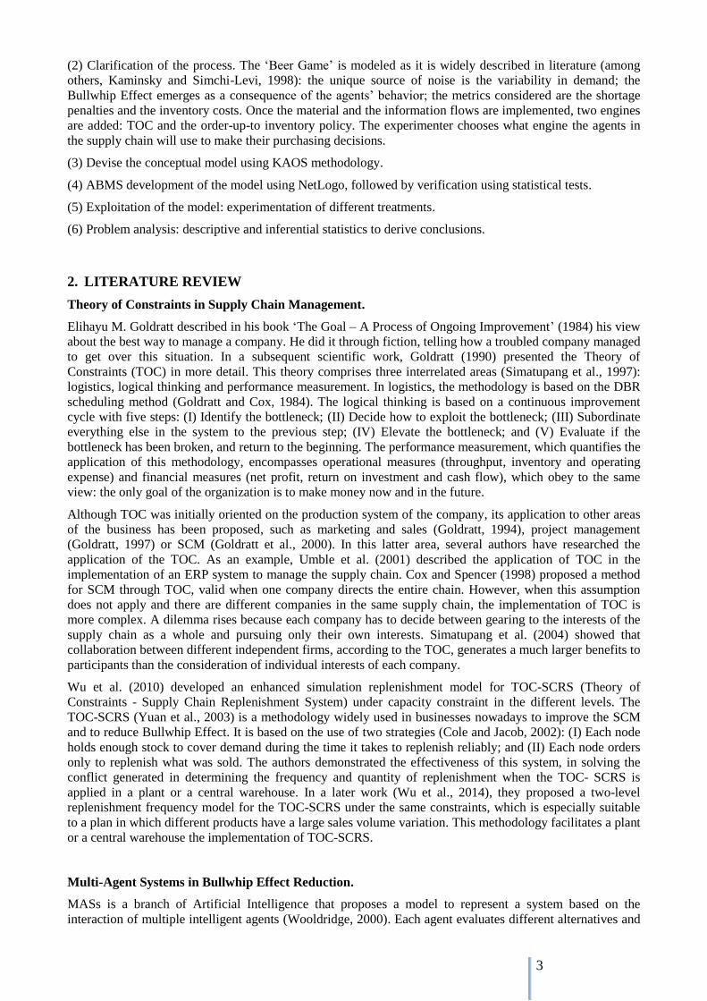
Applying Goldratt’s Theory of Constraints to reduce the Bullwhip Effect through Agent-Based Modeling José Costas 1 , Borja Ponte 2,* , David de la Fuente 2 , Raúl Pino 2 and Julio Puche 3 1 Polytechnic Institute of Viana do Castelo, School of Business Sciences of Valença Avenida Miguel Dantas, 4930-678, Valença, Portugal [email protected] 2 University of Oviedo, Department of Business Administration, Polytechnic School of Engineering Campus de Viesques s/n, 33204, Gijón, Spain {ponteborja, david, pino}@uniovi.es 3 University of Burgos, Department of Applied Economics, Faculty of Economics and Business Plaza Infanta Doña Elena s/n, 09001, Burgos, Spain [email protected] Abstract In the current environment, Supply Chain Management (SCM) is a major concern for businesses. The Bullwhip Effect is a proven cause of significant inefficiencies in SCM. This paper applies Goldratt’s Theory of Constraints (TOC) to reduce it. KAOS methodology has been used to devise the conceptual model for a multi-agent system, which is used to experiment with the well known ‘Beer Game’ supply chain exercise. Our work brings evidence that TOC, with its bottleneck management strategy through the Drum-Buffer-Rope (DBR) methodology, induces significant improvements. Opposed to traditional management policies, linked to the mass production paradigm, TOC systemic approach generates large operational and financial advantages for each node in the supply chain, without any undesirable collateral effect. Keywords: Bullwhip Effect; Drum-Buffer-Rope; KAOS modeling; Multi-agent Systems; Supply Chain Management; Theory of Constraints. 1. INTRODUCTION The complexity and dynamism that characterize the context in which companies operate nowadays have drawn a new competitive environment. In it, the development of information technologies, the decrease in transport costs and the breaking down of barriers between markets, among other reasons, have led to the perception that competition between companies is no longer constrained to the product itself, but it goes much further. For this reason, the concept of Supply Chain Management (SCM) has gained a lot of strength to the point of having a strategic importance. The current global economic crisis, consequence of many relevant systemic factors due to the fact that globalization still has not been able to develop systemic dynamic properties to deal with a growing variety of requirements, is creating conditions which increase awareness to adopt new approaches to make business (among others, Schweitzer et al., 2009); hence, SCM is a boiling area for innovation. Analyzing the supply chain, Forrester (1961) noted that changes in demand are significantly amplified along the system, as orders move away from the client. It was called the Bullwhip Effect. He studied the problem from the perspective of system dynamics. This amplification is also evidenced in the famous ‘Beer Game’ (Sterman, 1989), which shows the complexity of SCM. He concluded that the Bullwhip Effect is generated from local-optimal solutions adopted by supply chain members. This can be considered as a major cause of inefficiencies in the supply chain (Disney et al., 2005), because it tends to increase storage, labor, inventory, shortage and transport costs. Lee et al. (1997) identified four root causes in the generation of Bullwhip Effect in supply chains: (1) wrong demand forecasting; (2) grouping of orders into batches; (3) fluctuation in the products prices; and (4) corporate policies regarding shortage. The same idea underlies behind all of them: * Corresponding author. Tel. +34 985 13 34 73; Mob. +34 695 436 968.
Transcript of Applying Goldratt’s Theory of Constraints to reduce the ... Goldratt's TOC to Reduce the... ·...

Applying Goldratt’s Theory of Constraints to reduce
the Bullwhip Effect through Agent-Based Modeling
José Costas1, Borja Ponte2,*, David de la Fuente2, Raúl Pino2 and Julio Puche3
1Polytechnic Institute of Viana do Castelo, School of Business Sciences of Valença
Avenida Miguel Dantas, 4930-678, Valença, Portugal
2University of Oviedo, Department of Business Administration, Polytechnic School of Engineering
Campus de Viesques s/n, 33204, Gijón, Spain
{ponteborja, david, pino}@uniovi.es
3University of Burgos, Department of Applied Economics, Faculty of Economics and Business
Plaza Infanta Doña Elena s/n, 09001, Burgos, Spain
Abstract
In the current environment, Supply Chain Management (SCM) is a major concern for businesses. The
Bullwhip Effect is a proven cause of significant inefficiencies in SCM. This paper applies Goldratt’s Theory
of Constraints (TOC) to reduce it. KAOS methodology has been used to devise the conceptual model for a
multi-agent system, which is used to experiment with the well known ‘Beer Game’ supply chain exercise. Our
work brings evidence that TOC, with its bottleneck management strategy through the Drum-Buffer-Rope
(DBR) methodology, induces significant improvements. Opposed to traditional management policies, linked
to the mass production paradigm, TOC systemic approach generates large operational and financial
advantages for each node in the supply chain, without any undesirable collateral effect.
Keywords: Bullwhip Effect; Drum-Buffer-Rope; KAOS modeling; Multi-agent Systems; Supply Chain
Management; Theory of Constraints.
1. INTRODUCTION
The complexity and dynamism that characterize the context in which companies operate nowadays have
drawn a new competitive environment. In it, the development of information technologies, the decrease in
transport costs and the breaking down of barriers between markets, among other reasons, have led to the
perception that competition between companies is no longer constrained to the product itself, but it goes
much further. For this reason, the concept of Supply Chain Management (SCM) has gained a lot of strength
to the point of having a strategic importance. The current global economic crisis, consequence of many
relevant systemic factors due to the fact that globalization still has not been able to develop systemic
dynamic properties to deal with a growing variety of requirements, is creating conditions which increase
awareness to adopt new approaches to make business (among others, Schweitzer et al., 2009); hence, SCM is
a boiling area for innovation.
Analyzing the supply chain, Forrester (1961) noted that changes in demand are significantly amplified along
the system, as orders move away from the client. It was called the Bullwhip Effect. He studied the problem
from the perspective of system dynamics. This amplification is also evidenced in the famous ‘Beer Game’
(Sterman, 1989), which shows the complexity of SCM. He concluded that the Bullwhip Effect is generated
from local-optimal solutions adopted by supply chain members. This can be considered as a major cause of
inefficiencies in the supply chain (Disney et al., 2005), because it tends to increase storage, labor, inventory,
shortage and transport costs. Lee et al. (1997) identified four root causes in the generation of Bullwhip Effect
in supply chains: (1) wrong demand forecasting; (2) grouping of orders into batches; (3) fluctuation in the
products prices; and (4) corporate policies regarding shortage. The same idea underlies behind all of them:
* Corresponding author. Tel. +34 985 13 34 73; Mob. +34 695 436 968.

2
the transmission of faulty information to the supply chain. Therefore, the first approaches in the search for a
solution to this problem were based on trying to coordinate the supply chain. Some practices that have been
successfully implemented in companies are Vendor Managed Inventory (Andel, 1996), Efficient Consumer
Response (McKinsey, 1992) and Collaborative Planning, Forecasting and Replenishment (DesMarteu,
1998). Nevertheless, the Bullwhip Effect is still a major concern around operations management in the
supply chain. Chen and Lee (2012) discussed the linkage between the bullwhip measure and the supply chain
cost performance, capturing the essence of most-real world scenarios.
The Theory of Constraints (TOC) was introduced by Goldratt (1984) in his best seller 'The Goal',
representing a major innovation in the production approach. The author alleges that the sole purpose of an
organization is to make money now and in the future. Hereupon, the author defines six variables
as organizational measures to approach that goal. Three of them are operational: throughput, inventory and
operating expense. The other three are financial: net profit, return on investment and cash flow. All these
metrics are bound together through relationships. According to TOC, the most important thing to improve
the overall system performance is to concentrate the whole improvement effort on its bottleneck. Goldratt
proposes the Drum-Buffer-Rope (DBR) methodology to manage the system. Once the bottleneck is
identified, it becomes the drum of the system. A buffer is used to protect against variability in replenishment
time, because we aim to exploit the full capacity in the bottleneck. A rope is used to subordinate the system
to the bottleneck.
The major contribution of this paper is to provide evidence via a multi-agent simulation model about the
sound impact of TOC application to reduce the Bullwhip Effect in supply chains. TOC is compared against a
traditional management alternative, typical in mass production paradigm: the order-up-to inventory policy.
Our aim is to demonstrate that supply chains have plenty of reasons to operate according to the TOC
systemic approach. Figure 1 depicts the structure of our work.
Figure 1 – Structure of this work.
The conceptual multi-agent model has been worked out using KAOS methodology. Robust SW engineering
and test driven development techniques have been applied to build and verify the model. A multi-agent
system (MAS) is an optimal environment to address this issue, as it is a physically distributed problem,
where each node has only a partial knowledge about the problem-world.
As shown in figure 1, our research method has been the following:
(1) Definition of problem world (‘Beer Game’ supply chain) and problem statement (Bullwhip Effect).
3
(2) Clarification of the process. The ‘Beer Game’ is modeled as it is widely described in literature (among
others, Kaminsky and Simchi-Levi, 1998): the unique source of noise is the variability in demand; the
Bullwhip Effect emerges as a consequence of the agents’ behavior; the metrics considered are the shortage
penalties and the inventory costs. Once the material and the information flows are implemented, two engines
are added: TOC and the order-up-to inventory policy. The experimenter chooses what engine the agents in
the supply chain will use to make their purchasing decisions.
(3) Devise the conceptual model using KAOS methodology.
(4) ABMS development of the model using NetLogo, followed by verification using statistical tests.
(5) Exploitation of the model: experimentation of different treatments.
(6) Problem analysis: descriptive and inferential statistics to derive conclusions.
2. LITERATURE REVIEW
Theory of Constraints in Supply Chain Management.
Elihayu M. Goldratt described in his book ‘The Goal – A Process of Ongoing Improvement’ (1984) his view
about the best way to manage a company. He did it through fiction, telling how a troubled company managed
to get over this situation. In a subsequent scientific work, Goldratt (1990) presented the Theory of
Constraints (TOC) in more detail. This theory comprises three interrelated areas (Simatupang et al., 1997):
logistics, logical thinking and performance measurement. In logistics, the methodology is based on the DBR
scheduling method (Goldratt and Cox, 1984). The logical thinking is based on a continuous improvement
cycle with five steps: (I) Identify the bottleneck; (II) Decide how to exploit the bottleneck; (III) Subordinate
everything else in the system to the previous step; (IV) Elevate the bottleneck; and (V) Evaluate if the
bottleneck has been broken, and return to the beginning. The performance measurement, which quantifies the
application of this methodology, encompasses operational measures (throughput, inventory and operating
expense) and financial measures (net profit, return on investment and cash flow), which obey to the same
view: the only goal of the organization is to make money now and in the future.
Although TOC was initially oriented on the production system of the company, its application to other areas
of the business has been proposed, such as marketing and sales (Goldratt, 1994), project management
(Goldratt, 1997) or SCM (Goldratt et al., 2000). In this latter area, several authors have researched the
application of the TOC. As an example, Umble et al. (2001) described the application of TOC in the
implementation of an ERP system to manage the supply chain. Cox and Spencer (1998) proposed a method
for SCM through TOC, valid when one company directs the entire chain. However, when this assumption
does not apply and there are different companies in the same supply chain, the implementation of TOC is
more complex. A dilemma rises because each company has to decide between gearing to the interests of the
supply chain as a whole and pursuing only their own interests. Simatupang et al. (2004) showed that
collaboration between different independent firms, according to the TOC, generates a much larger benefits to
participants than the consideration of individual interests of each company.
Wu et al. (2010) developed an enhanced simulation replenishment model for TOC-SCRS (Theory of
Constraints - Supply Chain Replenishment System) under capacity constraint in the different levels. The
TOC-SCRS (Yuan et al., 2003) is a methodology widely used in businesses nowadays to improve the SCM
and to reduce Bullwhip Effect. It is based on the use of two strategies (Cole and Jacob, 2002): (I) Each node
holds enough stock to cover demand during the time it takes to replenish reliably; and (II) Each node orders
only to replenish what was sold. The authors demonstrated the effectiveness of this system, in solving the
conflict generated in determining the frequency and quantity of replenishment when the TOC- SCRS is
applied in a plant or a central warehouse. In a later work (Wu et al., 2014), they proposed a two-level
replenishment frequency model for the TOC-SCRS under the same constraints, which is especially suitable
to a plan in which different products have a large sales volume variation. This methodology facilitates a plant
or a central warehouse the implementation of TOC-SCRS.
Multi-Agent Systems in Bullwhip Effect Reduction.
MASs is a branch of Artificial Intelligence that proposes a model to represent a system based on the
interaction of multiple intelligent agents (Wooldridge, 2000). Each agent evaluates different alternatives and
4
makes decisions, in a clearly defined context, through local and external constraints. De la Fuente and
Lozano (2007) defend this methodology in the study of SCM, based on its own characteristics: it is a
physically distributed problem; it can be described a general pattern in decision-making; each agent can
consider both individual and chain interests; and it is a highly complex problem, which is influenced by the
interaction of many variables. For this reason, since the work of Fox et al. (1993), who were pioneers in
representing the supply chain as a network of intelligent agents, many studies have followed this line.
Maturana et al. (1999) used the multi-agent architecture to create the Metamorph tool. It was aimed at
facilitating the SCM in business through the introduction of intelligence in the design and manufacturing
stage. Later Kimbrough et al. (2002) studied the agent’s capability of managing their own supply chain. The
authors concluded that they can determine the most appropriate policy for each level, achieving a large
reduction in the Bullwhip Effect generated along the system. Some years later, Mangina and Vlachos (2005)
designed a smart supply chain in the food sector. They demonstrated that agents increase the supply cain’s
flexibility, information access and efficiency. Liang and Huang (2006) developed a MAS to forecast the
demand along a supply chain where each level has a different inventory policy. To calculate the forecast,
they used a genetic algorithm. Fuzzy logic was introduced into the analysis by Zarandi et al. (2008). The
authors constructed an agent-based system for SCM in dim environments. One of the latest studies on the
subject is the one by Saberi et al. (2012), who analyzed the chain collaboration. In their work, the agents
coordinate to make forecasts, to control the stock and to minimize total costs. Recently, Chatfield and
Pritchard (2013) constructed a hybrid model of agents and discrete simulation in order to represent the
supply chain. It was studied in several scenarios and they showed that returns of excess goods increase
significantly the Bullwhip Effect.
The literature review leads us to conclude that multi-agent methodology is widely used to experiment around
complex systems, such as supply chains. More specifically, it contains several works which apply these new
technologies to analyze the well-known problem of the Bullwhip Effect. Likewise, the application of TOC
has been studied to improve the management in complex systems, including supply chains. However, the
authors are aware of multiple real supply chains and know it is not common to apply Goldratt's theory. The
systemic thinking prompts the actors to solve a major dilemma, which consists on that the methods of
measurement, linked to reward and punishment policies, in the supply chain are not usually defined from a
systemic perspective, but from the relationships between each pair of nodes in the chain. Therefore, our aim
is to compare the holistic TOC method against a traditional reductionist alternative –the ‘order-up-to’
inventory policy– from a multi-agent approach.
3. PROBLEM FORMULATION
The Bullwhip Effect gained much importance when, in the early 90's, Procter & Gamble noticed that their
demand for Pampers diapers suffered considerable variations throughout the year, which did not correspond
to the relatively constant demands of its distributors –in addition, the swings of its suppliers were greater
(Lee et al., 1997). Since then, this phenomenon has been a fruitful research area within logistics studies.
Nevertheless, at present, it is one of the main concerns for business regarding to SCM. As way of example,
Buchmeister et al. (2012) illustrate this phenomenon using real data in three simulation cases of a supply
chain with different level constraints (production and inventory capacities).
In our study, we have considered a traditional single-product supply chain with a linear structure, composed
of five levels: client, shop retailer, retailer, wholesaler and factory, as the one used in the ‘Beer Game’.
Among the levels, there are two main flows: the material flow (related to the shipping of the product) from
the factory to the client, and the information flow (related to sending the orders) from the client to the
factory. Thus, there are five main actors. Four of them (shop retailer, retailer, wholesaler and factory) are
responsible for managing the supply chain, in order to meet the other’s (customer) needs.
The only purpose of the supply chain is, according to TOC, to make money, now and in the future. To assess
the approximation of a company to this goal, the author proposes three financial metrics: net profit, return on
investment (ROI) and cash flow. These metrics must be understood as complementary indicators. Thereby,
improving the SCM requires the simultaneous increase of the three values. The next question is: how can the
supply chain achieve it? Then, a second level of goals appears: (I) improve customer satisfaction; (II)
improve the efficiency of the supply chain; and (III) improve the utilization of the capacity.

5
Here, we can link our analysis with the TOC, considering three operational metrics: throughput (the rate at
which system generates money through sales), inventory (money invested in purchasing items intended to be
sold) and operating expense (money spent in order to turn inventory into throughput). Customer satisfaction
is a big contributor to throughput; increased efficiency means a decrease in operating expense; and
improving capacity usage implies achieving good results in the inventory. This operational metrics can also
be used to quantify the results of the supply chain, as the financial ones can be understood as a direct
consequence of these.
How do we attain these three goals of the second level? To increase customer satisfaction, the key element is
minimizing missing sales. Our model does not consider the effect of other factors, such as marketing. The
client will be satisfied if he finds what he needs in the shop retailer when he needs. To improve supply
efficiency and capacity utilization, the chain needs to reduce the Bullwhip Effect that causes an amplification
of the demands variability of levels upstream, which hinders both transportation and inventory management.
Thus, the decrease of the Bullwhip Effect brings the system to improve its operational, and consequently,
financial metrics.
Many authors quantify the Bullwhip Effect in a level n of the supply chain as the quotient between the
variance of the purchase orders launched (𝜎𝑃𝑂𝐸2 𝑛
) and the variance of the purchase orders received (𝜎𝑃𝑂𝑅2 𝑛
),
adjusted both the numerator and denominator by the mean value (𝜇𝑃𝑂𝐸𝑛, 𝜇𝑃𝑂𝑅
𝑛), according to equation 1.
For stationary random signal, in a linear supply chain, over longs periods of time, both means values are the
same. It should be noted that the purchase orders received by the shop retailer are the sales orders, which
meet the demand of the customer, and that purchase orders emitted by the upper level of the supply chain
(factory) translate in their own production. As the purchase orders launched by each level are the sale orders
received by the next one, the total Bullwhip Effect generated in the supply chain (𝐵𝐸𝑜𝑟𝑑𝑒𝑟𝑠𝑠𝑐) can be
expressed as the product of the Bullwhip Effect in the four different levels, by equation 2. When this ratio is
higher than 1, there is Bullwhip Effect in the supply chain.
𝐵𝐸𝑜𝑟𝑑𝑒𝑟𝑠𝑛 =
𝜎𝑃𝑂𝐸2 𝑛
/𝜇𝑃𝑂𝐸𝑛
𝜎𝑃𝑂𝑅2 𝑛
/𝜇𝑃𝑂𝑅𝑛=𝜎𝑃𝑂𝐸2 𝑛
𝜎𝑃𝑂𝑅2 𝑛 (1)
𝐵𝐸𝑜𝑟𝑑𝑒𝑟𝑠𝑠𝑐 =∏𝐵𝐸𝑜𝑟𝑑𝑒𝑟𝑠
𝑛
4
𝑛=1
(2)
This is a useful measure to quantify the evolution of orders, but only compares output variance with input
variance, and does not describe the structure that causes the variation increase. For this reason, some authors
(among others, Disney and Towill, 2003) also recommend the use of an alternative measure of the Bullwhip
Effect at each level n of the supply chain (𝐵𝐸𝑖𝑛𝑣𝑒𝑛𝑡𝑜𝑟𝑦𝑛), which quantifies fluctuations in actual inventory. It
can be expressed as the quotient of the variance of the stock (𝜎𝑆𝑇𝑂𝐶𝐾2 𝑛
) and the variance of the demand
(𝜎𝑃𝑂𝑅2 𝑛
), by means of equation 3. It is important to note that they are complementary measures. That is to
say, to improve the SCM is necessary to reduce the two of them, and not just one at the expense of the other.
𝐵𝐸𝑖𝑛𝑣𝑒𝑛𝑡𝑜𝑟𝑦𝑛 =
𝜎𝑆𝑇𝑂𝐶𝐾2 𝑛
𝜎𝑃𝑂𝑅2 𝑛 (3)
The goals of this level face two major obstacles of the SCM: uncertainty in both demand and lead time.
Uncertainty in the final customer demand is modeled through various statistical distributions. Lead time is
modeled constant, as stated in the ‘Beer Game’. Obviously, if orders lead time and material lead time were
both null, the supply from the factory would instantly respond to customer requirements and Bullwhip Effect
would not rise. The only relevant controllable factor (parameter) in our model is the engine to be used by
agents to make their purchasing decisions. For the sake of simplicity, we have not considered other causes
of the Bullwhip Effect, as the uncertainty in the lead time or variation in prices.
Figure 2 points out the p-diagram (parameter diagram –a widely used tool in robust engineering) that we
have used to establish the perimeter of our study. In it, we can see the overall supply chain function, the
noise sources that threaten the system function, and the parametric space, which are controllable factors
either at engineering stage or manufacturing stage.

6
Figure 2 – P-diagram of the system that we have developed.
4. DESCRIPTION OF THE MULTI-AGENT SYSTEM
We have used KAOS methodology (Dardenne et al., 1993) for the conceptual design. It is an engineering
methodology that joins, in the development of a software application, the overall objective that should be
met and the specific requirements that should be considered. This methodology relies on the construction of
a requirement model, whose graphical part can be represented by means of the KAOS Goal Diagram. Figure
3 shows the KAOS Goal Diagram that we have created and used in the development of the system.
TOC approach consists on managing the supply chain based on the bottleneck. This is one of the foundations
of the TOC: any improvement that is deployed away from the bottleneck of a system represents a waste of
resources. Therefore, this fact leads to a new question: Where is the bottleneck in this supply chain? The
factory would be the bottleneck if its production rate cannot cover the customer demand. But the factory has
not a capacity constraint in the ‘Beer Game’. The intermediate nodes, wholesaler and retailer, could be the
bottleneck if its storage or transport capacity did not allow the supply chain to meet the final demand, but
this is not the situation that we have considered. So, the bottleneck is the final customer demand. To
maximize the flow at the bottleneck means to have zero missing sales at the shop retailer. Therefore, the
drum is placed at the shop retailer.
Each time that a demand event is triggered to the system, the drum makes all the agents react. Each agent
(node) calculates its rope length to the drum position and makes the order decision based on its downstream
buffer to the bottleneck. Instead of traditional safety stock based on material quantities, TOC-based buffers
are a function of the lead time. Buffer management consists on moving the flow so that arrival happens on
time at the bottleneck. Because the shop retailer is the drum, this agent looks for maximizing flow; which
means preventing missing sales by linking the final customer demand forecast straight to the factory. All
other nodes work subordinated to the drum with a shipping rope.
Each node works using a finite state machine schema. The agent is idle until the drum triggers it. From the
idle state it switches to serve backorders state. Then, it flows to the shipping orders state. Once the agent has
moved material downstream, it moves to the sourcing state (take care of information flow). Finally the agent
moves to the reporting state, when it cares about updating and exporting information. And then the agent
switches now to the idle state to reiterate the loop. The state transition diagram is represented in figure 4.

7
Figure 3 – KAOS Goal Diagram of our MAS.
Figure 4 – State transition diagram (local for each agent).
Some details about our simulation engine should be commented. The simulation clock advances based on a
FEL (future event list). Events are scheduled in the future and the clock advance will move to the event
which is sooner due. Every takt (block of time between two consecutive arrivals of customers to the shop
retailer) schedules the next one. Each customer arrival schedules new events in the FEL so to divide each
time bucket into small time windows. Synchronizing mechanisms are used to force nodes to follow a
downstream sequence for material flow and an upstream sequence for the orders flow.
During these sequences agents transition their states to perform all the activities: move material downstream,
move orders upstream, serve backorders just in case, serve the current order, place backorder if needed, place
its purchase order upstream (according to the settings for the order policy), and report data into the export
file. Of course the system behaves polymorphous depending on the setting of the experiment. This means
that details of what each node does at each state follows the appropriate rules linked to the parameters given
at the setup stage.

8
We have used robust SW engineering techniques (Taguchi, 2000) to build the model and NetLogo 5.0.5 to
implement it. Figure 5 shows a screenshot of the interface window of the implemented model. The interface
window provides the experimenter with the animation frame, the controls to setup parameters and to run
each experiment, and the graphics and monitoring stuff to track what the system is doing. NetLogo provides
two additional windows, one for the model documentation and another for the model code.
In the next paragraphs we will clarify some relevant details about what the system does when operating
under TOC parameters and when the order-up-to policy is the selection made by the experimenter.
Figure 5 – Screenshot of the system interface at one particular moment of the simulation.
Order-up-to inventory policy.
This policy is implemented as follows: at the end of each period t, the shop retailer, retailer, wholesaler and
factory update the forecast (𝐷�̂�) based on the demand or order received, by means of a moving average of the
last three observations (𝐷𝑡−𝑖), according to equation 4. In this policy, under the assumption of normal
demand, the order-up-to point (𝑦𝑡) is estimated as the product of the forecast and the lead time (𝐿), plus a
term related to the safety stock (equation 5). It depends on a parameter (𝑍) that is a function of the security
level and the standard deviation of the error (𝑆𝑡). We have used 𝑍 = 1.64 in order to work with a confidence
level of 95%. The purchase order quantity for each period is the difference between the order-up-to point of
this period and the previous one, plus the demand of the previous period, by equation 6. Note that the
purchase order arrives at the start of period t+L and sales orders are filled at the end of each period. More
information about this management policy can be found in Chen et al. (2003). In our case, we have used a
three period moving average to calculate the forecast.
𝐷�̂� =1
𝑛∙∑𝐷𝑡−𝑖
𝑛
𝑖=1
(4)
𝑦𝑡 = 𝐿 ∙ 𝐷�̂� + 𝑍 ∙ √𝐿 ∙ 𝑆𝑡 = 𝐿 ∙ 𝐷�̂� + 𝑍 ∙ √𝐿 ∙ √1
𝑛∙∑(𝐷𝑡−𝑖 − 𝐷𝑡−𝑖̂ )2
𝑛
𝑖=1
(5)
𝑞𝑡 = 𝑦𝑡 − 𝑦𝑡−1 + 𝐷𝑡−1 = (1 +𝐿
𝑛) ∙ 𝐷𝑡−1 − (
𝐿
𝑛) ∙ 𝐷𝑡−(𝑛+1) + 𝑍 ∙ √𝐿 ∙ (𝑆𝑡 − 𝑆𝑡−1) (6)

9
DBR methodology - Goldratt’s TOC policy.
The DBR methodology has been implemented according to the Goldratt’s TOC, summarized in section 2 and
following to the meta-model explained above. We should remember that, in the context we are considering,
the shop retailer is the constraint in the system, so it must be the drum. The aim of the solution is to protect
it, and therefore the supply chain as a whole, against process dependency and variation, and thus to optimize
the system. In these circumstances, the other levels must be subordinated to the shop retailer. The buffer is
the material release duration and the rope is the release timing. Kelvyn Youngman (2009) has developed an
outstanding guide for the implementation of the TOC in systems of very different kinds, which can be
consulted to get further detail in the process described below.
In the TOC mode, the system operates in two stages. In the first one, the systemic condition to tie the
different levels of the supply chain through time (and not by product) is established. It is the planning stage
and it is orientated to operate the system as a whole. In the second one, the buffer is administered along the
intermediate stations, to guide the way in which the motor is tuned for peak performance. It is the control
stage that allows us to keep a running check on the system performance. The idea is summarized in figure 6.
Figure 6 – Two-stage based operation system.
With the previous objective, at each time unit, the factory uses the history of the demand in the shop retailer
(the time interval defined by the rope, which is the period of time to protect), in order to decide the
production orders that must be placed in the channel (the manufacturing time is equal to the lead time in the
remaining levels: 3 periods). Subsequently, each node of the supply chain, except the shop retailer (as no
other level can be found downstream) manages the buffer. The horizontal channels are the buffer of the
model. The buffer is time and material flow, but not the order flow. Manage it means compensating in each
takt the flow dissipated downstream after shipping. Therefore, for example, in the case of the factory, the
buffer is 9 time units (lead time of 3 units in the previous three levels). Unlike classical policies, the TOC
orders are dosage orders into the buffer and they are dissipative. They have no lead time, because each agent
decides what to dose subordinated to the bottleneck. They do not generate backorders, as the next dosage
again obey the bottleneck. Figure 7 graphically represents this idea, showing the drum, the buffer and the
rope.
Figure 7 – Schematic representation of the MAS when it works according to the TOC.

10
5. SIMULATION STUDY AND CONCLUSIONS
As the equations related to the inventory policy that we have used to contrast the results are based on the
assumption of normal demand, we have simulated the customer demand through a normal distribution with a
mean of 12. We have performed treatments on three different scenarios: when the variability is low (standard
deviation of 1; coefficient of variation 8.3%), when the variability is moderate (standard deviation of 3;
coefficient of variation 25.0%), and when the variability is high (standard deviation of 5; coefficient of
variation 41.7%), in order to extend the conclusions considering the effect of the demand variability in the
SCM. Thus, our experimentation approach, can be written as shown in equation 7, where 𝑌 is a vector of the
key performance indicators (in terms of Bullwhip Effect); 𝑋 is the policy management, which is a nominal
attribute variable (order-up-to inventory policy or DBR methodology); 𝑍 is an external noise condition,
which is characterized for de experiment as 𝑁(12, 𝜎), where 𝜎 is set to three different levels in order to
represent different levels of variability with respect to the average demand; and 𝜉 represents the residuals –
the unexplained part of the system response.
𝑌 = 𝑓(𝑋, 𝑍) + 𝜉 (7)
So, it is a full DoE (Design of Experiments) with two factors. One factor (order policy) is controllable and is
taken at two levels; while the other factor (demand law) is noise and enters the simulated experiment at three
levels. This idea is shown in table 1.
Factor Level Treatment Demand Law (Z) Order Policy (X)
Demand Law Normal(12,1) 1 Normal(12,1) Order-up-to inv. pol.
(Z) Normal(12,3) 2 Normal(12,3) Order-up-to inv. pol.
Normal(12,5) 3 Normal(12,5) Order-up-to inv. pol.
4 Normal(12,1) DBR methodology Order Policy Order-up-to inv. pol. 5 Normal(12,3) DBR methodology
(X) DBR methodology 6 Normal(12,5) DBR methodology
Table 1 – DoE (Design of Experiments) table
A time horizon of 330 periods was used for each treatment. The first 30 are discarded as warm-up period, so
to avoid the initial transitory that can alter the results. On the other hand, the 300 remainder periods is a large
enough time interval to check stability according to the common practices.
Model verification and validation.
A fundamental step in any modeling process is the verification of the model, with the aim of checking its
cohesion and consistency; that is, to check that the development matches the logic of the conceptual design.
This model was created following strict rules of clean code, test driven development focus, versioning for
continuous functionality increments, and it uses failure modal analysis in order to prevent failures. Although
these good practices of software engineering reduce the probability of error, they do not eliminate it
completely. Therefore, we have complemented it with mechanics (exception handling, cross checking, police
agents for system audits) for early detection of any system malfunction.
Another essential step in simulation process is the validation phase. The experimenter wants model
predictions to match reasonably well the reality, so that the simulation model is useful to devise changes and
apply them to improve the real system. To validate our model we have used factory acceptance test (FATs),
so to confirm that the model exhibits a well known behavior when exposed to controlled conditions. As an
example, we include one this kind of tests that are implemented in the model.
Test conditions: (I) Constant demand in the shop retailer: 12 sku / period.
(II) Damaged equipment on the factory: zero production.
Expected behavior: (I) It only serves customers until the initial stock is depleted.
(II) Cumulative backorders are generated at each node.
Acceptance criteria: (I) Demand turns into missing sales (12 sku / period) in steady state.
(II) Storage costs are zero in steady state.
Once the FAT tests were satisfactory, the standard approach was used when comparing treatments under
stochastic conditions: each treatment is replicated (it was run three times) so that the statistical analysis takes
into account the experimental error. An overall stability study (run several trajectories –replicas– of each

11
experimental treatment) about the key output metrics (lost sales, stocks) was also conducted. And, of course,
we did care about the experimental error (using replicas and hypothesis testing).
The model statistically probed to be valid: matched expected outputs under controlled scenarios, reached
stability and have repeatability.
Analysis of the treatments.
Tables 2, 3, 4 and 5 report the final results of the treatments, both the outcomes exported from the simulation
(process metrics) and the results of the simulations in terms of Bullwhip Effect and missing sales
(performance metrics).
Process Metrics
Scenario 1
Low variability
[Treatment 1]
Scenario 2
Mid variability
[Treatment 2]
Scenario 3
High variability
[Treatment 3]
Consumer Demand 11.98 – 1.04 11.97 – 7.97 11.91 – 27.61
Shop Retailer Purchase Orders 11.47 – 98.39 11.49 – 133.53 11.64 – 232.13
Retailer Purchase Orders 12.04 – 380.20 11.79 – 715.74 12.50 – 1008.79
Wholesaler Purchase Orders 11.79 – 1405.58 13.17 – 1994.30 13.47 – 3304.94
Factory Production 12.08 – 4247.31 14.15 – 4162.65 13.03 – 7228.66
Shop Retailer Inventory 12.0 – 101.1 19.2 – 215.9 34.9 – 613.6
Retailer Inventory 67.9 – 1011.38 105.1 – 4429.3 154.5 – 8362.3
Wholesaler Inventory 218.9 – 13471.1 384.1 – 22900.2 559.9 – 51286.0
Factory Inventory 577.7 – 32599.2 593.1 – 13674.0 1057.0 – 137635.3
Table 2 – Results of the tests when the order-up-to inventory policy is used (I): Mean (left) and variance (right) of the consumer demand, purchase
orders, factory production and inventory in the different levels of the supply chain (without warm-up time).
Performance Metrics
Scenario 1
Low variability
[Treatment 1]
Scenario 2
Mid variability
[Treatment 2]
Scenario 3
High variability
[Treatment 3]
Shop Retailer Bullwhip Effect [Orders] 99.13 17,47 8.60
Retailer Bullwhip Effect [Orders] 3.68 5,22 4.05
Wholesaler Bullwhip Effect [Orders] 3.78 2,49 3.04
Factory Bullwhip Effect [Orders] 2.95 1,94 2.26
Supply Chain Bullwhip Effect [Orders] 4063.14 442.07 239.33
Shop Retailer Missing Sales [sku] 163 124 86
Shop Retailer Bullwhip Effect [Inventory] 97.58 27,10 22.22
Retailer Bullwhip Effect [Inventory] 10.28 33,17 36.02
Wholesaler Bullwhip Effect [Inventory] 35.43 32,00 50.84
Factory Bullwhip Effect [Inventory] 23.19 6,86 41.65
Table 3 – Results of the tests when the order-up-to inventory policy is used (II): Orders Bullwhip Effect and Inventory Bullwhip Effect generated along the different levels, in addition to missing sales to evaluate the performance of the supply chain (without warm-up time).
Tables 2 and 3 demonstrate the huge generation of Bullwhip Effect along the supply chain when using the
order-up-to inventory policy. Whilst the quantity order average remains constant along the supply chain
nodes (it only varies slightly due to missing sales and inventory accumulation), the quantity order variance
increases greatly as we move upstream. It is interesting to see that the average inventory increases
dramatically upstream the chain. Nevertheless, the amount of missing sales is noteworthy. As a conclusion,
with the order-up-to policy the service level to customers is not extremely bad (still, it is not excellent), and
the weak point is that this bad service is obtained at a huge cost in terms of inventory. The lesson learnt, and
it is very usual in the marketplace, is that the customer service is protected with huge inventory and this
policy is not effective, because the root cause of the problems is not being considered. According to the
industrial experience of the authors, this is a very common finding in ailing processes.
Looking at these tables, it can be seen that the greatest Bullwhip Effect is generated, according to the
classical formulation, in the scenario of low variability. Obviously, the greater the variability in consumer
demand, the greater the variability in the rate of production of the factory. However, the relationship between
the two variances is much larger when the variability in consumer demand is low. Moreover, this classic
inventory management policy generates more missing sales when the variability of consumer demand is low.
At first glance, this result might seem surprising, but it is not, as the explanation lies in the level of

12
inventories: when the variability is very high, the levels of the supply chain tend to be overprotective. For
this reason, the missing sales are reduced at the expense of increasing the inventory far from the customer.
Process Metrics
Scenario 1
Low variability
[Treatment 4]
Scenario 2
Mid variability
[Treatment 5]
Scenario 3
High variability
[Treatment 6]
Consumer Demand 12.07 – 1.13 12.47 – 11.03 11.79 – 24.43
Shop Retailer Purchase Orders 12.10 – 9.11 13.04 – 75.82 12.83 – 134.10
Retailer Purchase Orders 12.10 – 7.32 12.33 – 58.37 11.66 – 101.48
Wholesaler Purchase Orders 12.09 – 5.63 12.36 – 53.60 11.47 – 110.75
Factory Production 12.09 – 7.98 12.47 – 76.48 11.39 – 145.03
Shop Retailer Inventory 9.2 – 12.5 16.8 – 74.1 21.9 – 142.9
Retailer Inventory 14.0 – 23.8 18.6 – 140.4 20.6 – 209.7
Wholesaler Inventory 50.7 – 17.2 56.5 – 190.7 59.3 – 523.7
Factory Inventory 97.1 – 18.0 113.6 – 162.0 121.0 – 441.1
Table 4 – Results of the tests when the DBR methodology is used (I): Mean (left) and variance (right) of the consumer demand, purchase orders,
factory production and inventory in the different levels of the supply chain (without warm-up time).
Performance Metrics
Scenario 1
Low variability
[Treatment 4]
Scenario 2
Mid variability
[Treatment 5]
Scenario 3
High variability
[Treatment 6]
Shop Retailer Bullwhip Effect [Orders] 8.02 6.57 5.05
Retailer Bullwhip Effect [Orders] 0.80 0.81 0.83
Wholesaler Bullwhip Effect [Orders] 0.77 0.92 1.11
Factory Bullwhip Effect [Orders] 1.42 1.42 1.32
Supply Chain Bullwhip Effect [Orders] 7.03 6.94 6.15
Shop Retailer Missing Sales [sku] 1 54 82
Shop Retailer Bullwhip Effect [Inventory] 11.01 6.72 5.85
Retailer Bullwhip Effect [Inventory] 2.61 1.85 1.56
Wholesaler Bullwhip Effect [Inventory] 2.34 3.27 5.16
Factory Bullwhip Effect [Inventory] 3.19 3.02 3.98
Table 5 – Results of the tests when the DBR methodology is used (II): Bullwhip Effect and Alternative Bullwhip Effect generated along the different levels, missing sales and Goldratt’s operational metrics to evaluate the performance of the supply chain (without warm-up time).
Tables 4 and 5 point out that the TOC also causes Bullwhip Effect in the supply system, since variability in
purchase orders increases and both the mean and the variance of the inventory level increment as they move
away from the consumer. However, a simple comparison of these tables with respect to tables 1 and 2 makes
clear the enormous effectiveness of DBR methodology in managing the supply chain. The amplification of
the variability of orders is much lower when the supply chain is managed according to the practices proposed
by Goldratt. Likewise, the TOC gets to manage the supply chain with minor inventories at all levels.
Moreover, despite that, the amount of missing sales decreases meaningfully. Hence, the important findings
using TOC approach is that both negative effects (Bullwhip Effect and missing sales) reduce at the same
time when compared to the order-up-to policy.
The generation of the Bullwhip Effect in the supply chain and the improvements introduced by Goldratt’s
practices in comparison with the traditional management policies can be shown graphically in many different
ways. For example, figure 8 exhibits the production rate of the factory throughout the time horizon for the
two tests assuming normal with mean 12 and standard deviation 3 in the final consumer. When the system
works according to the order-up-to inventory policy, the factory production varies greatly: in most periods, it
has no production needs while in some specific moments it must manufacture very high amounts of product.
With the DBR methodology, however, variability in the factory production is much lower, which translates
in cost savings from different perspective (among others, labor, inventory, and transportation costs).
Why does such amplification occur? When the supply chain is managed according to the order-up-to
inventory policy, the peaks in orders received for each level translate into an even bigger peak in orders
placed by that level. The time difference is the lead time. That is to say, each level contributes increasing the
distortion in the supply chain, and so decreasing the reliability of the transmitted information. When using
TOC, the supply chain performs dramatically better.
The other way to observe the Bullwhip Effect is through the inventory of the various levels. It is possible to
see it, for example, by means of box plots. Figure 9 shows these graphs, with the average, the indicators of
the first and third quartile and the upper and lower limits, for the stock of the different members of the supply

13
chain in tests with mean 12 and standard deviation 5. It should be noted that the values lower than 0 are
related to inventory backorders that will be met the following periods. It is enough to compare the vertical
scale of the two graphs to observe the improvements introduced by TOC, both in mean and in variance.
Figure 8 – Factory production in the two tests (order-up-to inventory policy and DBR methodology) carried out with a N(12,3).
Figure 9 – Box plots of the inventory level in the different members of the supply chain in the two tests (Order-up-to inventory policy and DBR
methodology) carried out with a N(12,5).
Statistical significance of results.
By looking at the plots shown above we have visual evidence that the supply chain performs much better
when using TOC, as commented. Nevertheless, it should be formally verified. The statistical tests were
conducted for the different treatments, although they are only shown in one case, by way of example.
First, we concentrate on missing sales at the shop retailer, which is the only point where the fact of missing
sales is really a critical concern. When the standard deviation of the demand is 5, we have the distribution for
the missing sales penalty in each time bucket (sample size N > 150, once excluded the warm-up period). We
have tested the null hypothesis “H0: missing sales mean = 0”. For the order-up-to inventory policy, using 1-
sample t test has a pValue less than 5%, which rejects null hypothesis. So, the penalty for missing sales is
significantly different from zero. On the other hand, running a same length trajectory with TOC, all time
buckets, after the warm-up period, have zero lost sales. The conclusion is that TOC policy effectively
protects the supply chain against losing sales, whilst this does not happen with the order-up-to policy.
Once we have got formal evidence that the supply chain performance significantly improves when applying
TOC in terms of external customer satisfaction (here, maximizing sales by exploiting the bottleneck), we
now take care of getting also formal evidence that this achievement is not at the expense of increasing
inventory cost in the overall supply chain. The inventory total cost has been collected during a long (for
example, 200 time buckets) period of time after the system warm-up, and proceed first to check is the
variance of this metric is unequal when using TOC versus when using order-up-to policy. We check, using a
2-variance test, the null hypothesis “H0: variance (total inventory cost in the supply chain) | policy = TOC)
= variance (total inventory cost in the supply chain) | policy = order-up-to)”. Figure 10 shows that in the
sample, the standard deviation statistic of the metric at TOC level is less than at order-up-to level; the Levene

14
test shows a p-value lower than 5%; so we reject null hypothesis. Therefore, TOC policy induces less
variance in the inventory cost (so, to the goal stock in the system).
Figure 10 also displays the Welch’s test to compare the means. Again, we reject the null hypothesis “H0:
mean (total inventory cost in the supply chain) | policy = TOC) = mean (total inventory cost in the supply
chain) | policy = order-up-to)”. And, we take the alternative hypothesis: the total inventory cost in the supply
chain is less when we use TOC policy. In conclusion, as expected, TOC not only gives a full protection
against missing sales (while order-up-to does not), but besides, TOC achieve this result even reducing the
total inventory cost (less variance and lower mean).
Figure 10 – Hypothesis contrast to the significant difference between the inventory costs and averages of both policies.
6. FINDINGS, RECOMMENDATIONS AND NEXT STEPS
The new competitive environment has granted the Supply Chain Management a strategic role in the search
for competitive advantage. For this reason, the orders variance amplification along the supply chain, known
as the Bullwhip Effect, is an important concern for businesses, as it is a major cause of inefficiencies.
Traditional management policies linked to the mass production paradigm, such as order-up-to inventory
policy, are unsuccessful ‒as already shown in literature‒ in terms of fighting the Bullwhip Effect.
KAOS methodology was used to devise the multi-agent simulation model carried out on this research. The
Gall’s incremental principle (a complex system that works properly has evolved from a simple system which
was effective) has been applied to end up with a highly reliable, self-controlled, tested and flexible model so
to experiment TOC approach versus order-up-to policies for managing a multi-echelon supply chain and
collect data evidence of system behavior. Statistical analysis have been applied to these data blocks taking
into account the warm-up period, stability study and the final hypothesis testing to raise our conclusions.
Our first finding was that the higher the final customer demand variability, the higher is the amplification
upstream the supply chain, because each node tends to overprotect itself due to the fear of breaking stock.
TOC philosophy has demonstrated in this work that is highly effective in remedying this issue. A dramatic
improvement in the overall supply chain has been reached in several explored levels of external demand
variability, but the more important point is that every level has improved its own performance by
subordinating to the bottleneck. Hence, the best solution for the system is the best solution for each
individual member.
The major contribution of this work has been to demonstrate that considering only the main effects, there are
enough reasons to manage the supply chain according to Goldratt's philosophy.
There are plenty of model extensions and future works that this research group is planning as next steps on
this fascinating topic.
(1) To analyze why, provided that TOC is a mature and validated theory, it is not yet widely used. We
wonder that moving the agents away from their natural egoist behavior needs some educational phases, and
simulation can play an important role here.

15
(2) To extend this model to a larger noise conditions scenario. Now the noise factors have been limited in
the model to include only different levels of variability in the external demand and to keep constant the
delays in the material and in the information flows. Of course, considering other disturbance factors like
scrap, variability in transportation delays, errors in the information flow and other sources of waste in the
supply chain, a comparison of system robustness using TOC versus other management policies can provide
insights to other relevant findings.
(3) To place SCM rules and controls to prevent selfish behavior of agents that could operate against the
supply chain major interests. We also plan to explore to what extent agents applying fuzzy logic decision in
their quest of local optima compares against applying holistic fuzzy logic decision making engines. Thereby,
the concept of the Nash Equilibrium in supply chains must be introduced.
(4) To model adaptive mechanisms on the supply chain in order to detect and react to bottleneck
displacements; for instance, due to changes in the storage technology, storage policies, multimodal
transportations costs and so forth.
Even though the shift in our production and management systems was initiated after World War II, with lean
manufacturing taking over the mass production paradigm, the systemic approach has spread in a very
irregular way. Agent-based modeling and simulation is an important tool to educate people, and to
contribute to create critical mass for a large deployment of the systemic approach, which in the end
translates in a better skilled population to deal with complex systems like supply chains.
ACKNOWLEDGEMENTS
The authors deeply appreciate the financial support provided by the Government of the Principality of
Asturias, through the ‘Severo Ochoa’ program (reference BP13011). We would also like to thank Professor
Isabel Fernández for making a valuable contribution to the discussion and for her interesting comments.
REFERENCES
Andel, T. (1996). Manage inventory, own information. Transportation & Distribution, 37(5), 54-58.
Buchmeister, B., Friscic, D., Lalic, B. & Palcic, I. (2012) Analysis of a Three-Stage Supply Chain with Level
Constraints. International Journal of Simulation Modelling, 11(4), 196-210.
Chatfield, D. C., & Pritchard, A. M. (2013). Returns and the bullwhip effect. Transportation Research Part E: Logistics
and Transportation Review, 49(1), 159-175.
Chen, F., Drezner, Z., Ryan, J. K., & Simchi-Levi, D. (2001). Quantifying the Bullwhip Effect in a Simple Supply
Chain: The Impact of Forecasting, Lead Times, and Information. Management Science, 46(3), 436-443.
Chen, L., Lee, H. L. (2012). Bullwhip Effect Measurement and its Implications. Operations Research, 60(4), 771-784.
Cole, H., & Jacob, D. (2003). Introduction to TOC supply Chain. AGI Institute.
Cox, J. F., & Spencer, M. S. (1998). The Constraints Management Handbook, Lucie Press, Boca Raton, FL.
Dardenne, A., Lamsweerde, A., & Fichas, S. (1993). Goal-directed requirements acquisition. Science of Computer
Programming, 20, 3-50.
De la Fuente, D., & Lozano, J. (2007). Application of distributed intelligence to reduce the bullwhip effect.
International Journal of Production Research, 44(8), 1815-1833.
DesMarteu, K. (1998). New VICS publication provides step-by-step guide to CPFR. Bobbin, 40(3), 10.
Disney, S. M., & Towill, D. R. (2003). On the bullwhip and inventory variance produced by an ordering policy. Omega
– The International Journal on Management Science, 31, 157-167.
Disney, S. M., Farasyn, I., Lambrecht, M., Towill, D. R., & Van de Velde, W. (2005). Taming the Bullwhip Effect
whilst watching customer service in a single supply chain echelon. European Journal of Operational Research, 173(1),
151-172.
Forrester, J. W. (1961). Industrial dynamics, MIT Press. Cambridge, MA.
Fox, M. S., Chionglo, J. F., & Barbuceanu, M. (1993). The Integrated Supply Chain Management System. Internal
Report, Dept. of Industrial Engineering, University of Toronto.

16
Goldratt, E. M. (1990). Theory of Constraints. North River Press, Croton-on-Hudson, NY.
Goldratt, E. M. (1994). It’s not Luck. North River Press, Great Barrington, MA.
Goldratt, E. M. (1997). Critical Chain. North River Press, Great Barrington, MA.
Goldratt, E. M., & Cox, J. (1984). The goal – A process of ongoing improvement. North River Press. Croton-on-
Hudson, NY.
Goldratt, E. M., Schragenheim, E., & Ptak, C. A. (2000). Necessary but not sufficient. North River Press. Croton-on-
Hudson, NY.
Kaminsky, P., & Simchi-Levi, D. (1998). A new computerized beer game: a tool for teaching the value of integrated
supply chain management. Supply Chain and Technology Management. Hau Lee and Shu Ming Ng Edts. The
Production and Operations Management Society. Miami, Florida.
Kimbrough, S. O., Wu, D. J., & Zhong, F. (2002). Computers play the beer game: can artificial manage supply chains?
Decision Support Sytems. 33, 323-333.
Lee, H. L., Padmanabhan, V., & Whang, S. (1997). The Bullwhip Effect in supply chains. MIT Sloan Management
Review, 38(3), 93-102.
Liang, W. Y., & Huang, C. C. (2006). Agent-based demand forecast in multi-echelon supply chain. Decision Support
Systems, 42(1), 390-407.
Mangina, E., & Vlachos, I. P. (2005). The changing role of information technology in food and beverage logistics
management: Beverage network optimization using intelligent agent technology. Journal of Food Engineering, 70(3),
403-420.
Maturana, F., Shen, W., & Norrie, D. H. (1999). MetaMorph: An adaptive agent-based architecture for intelligent
manufacturing. International Journal of Production Research, 37(10), 2159-2173.
McKinsey, J. (1992). Evaluating the impact of alternative store formats. Supermarket Industry Convention. Food
Marketing Institute, Chicago.
Saberi, S., Nookabadi, A. S., & Hejazi, S. R. (2012). Applying Agent-Based System and Negotiation Mechanism in
Improvement of Inventory Management and Customer Order Fulfillment in Multi Echelon Supply Chain. Arabian
Journal for Science and Engineering, 37(3), 851-861.
Schweitzer, F., Fagiolo, G., Sornette, D., Vega-Redondo, F., Vespignani, A., & White, D. R. (2009). Economic
Networks: The New Challenges. Science, 325 (5939), 422-425.
Simatupang, T. M., Wright, A. C., & Sridharan, R. (2004). Applying the Theory of Constraints to supply chain
colaboration. Supply Chain Management: An International Journal, 9(1), 57-70.
Simatupang, T. M., Hurley, S. F., & Evans A. N. (1997). Revitalizing TQM efforts: a self-reflection diagnosis based on
the Theory of Constraints. Management Decision, 35(10), 746-752.
Sterman, J. D. (1989). Modeling managerial behavior: Misperceptions of feedback in a dynamic decision making
experiment. Management Science, 35(3), 321-339.
Taguchi, G., Chowdhury, S., & Taguchi, S. (2000). Robust Engineering. Mc Graw – Hill, New York.
Umble, M., Umble, E., & von Deylen, L. (2001). Integrating enterprise resources planning and Theory of Constraints: a
case study. Production and Inventory Management Journal, 42(2), 43-48.
Wilensky, U. (1999). NetLogo. Northwestern University, Evanston, IL: The Center for Connected Learning and
Computer - Based Modeling. http://ccl.northwestern.edu/netlogo/ Last access 10 April 2014.
Wooldridge, M. (2000). Reasoning about Rational Agents. MIT Press, Cambridge, Mass.
Wu, H. H., Chen, C. P., Tsai, C. H., & Tsai, T. P. (2010). A study of an enhanced simulation model for TOC supply
chain replenishment system under capacity constraint. Expert Systems with Applications, 37, 6435-6440.
Wu, H. H., Lee, A. H. I., Tsai, T. P. (2014). A two-level replenishment frequency model for TOC supply chain
replenishment systems under capacity constraint. Computers & Industrial Engineering, 72, 152-159.
Youngman, K. (2009). A Guide to Implementing the Theory of Constraints (TOC). http://www.dbrmfg.co.nz/ Last
access 9 July 2014.
Yuan, K. J., Chang, S. H., & Li, R. K. (2003). Enhancement of theory of constraints replenishment using a novel
generic buffer management procedure. International Journal of Production Research, 41(4), 725-740.
Zarandi, M. H., Fazel, Pourakbar, M., & Turksen, I. B. (2008). A fuzzy agent-based model for reduction of bullwhip
effect in supply chain systems. Expert systems with applications, 34(3), 1680-1691.