Applied Technology Institute (ATIcourses.com) Stay Current In Your Field • Broaden Your Knowledge • Increase Productivity

349 Berkshire Drive • Riva, Maryland 21140888-501-2100 • 410-956-8805Website: www.ATIcourses.com • Email: ATI@ATIcourses.com

ATI Provides Training In:

• Acoustic, Noise & Sonar Engineering

• Communications and Networking

• Engineering & Data Analysis

• Information Technology

• Radar, Missiles & Combat Systems

• Remote Sensing

• Signal Processing

• Space, Satellite & Aerospace Engineering

• Systems Engineering & Professional Development

ATI Provides Training In:

• Acoustic, Noise & Sonar Engineering

• Communications and Networking

• Engineering & Data Analysis

• Information Technology

• Radar, Missiles & Combat Systems

• Remote Sensing

• Signal Processing

• Space, Satellite & Aerospace Engineering

• Systems Engineering & Professional Development

Check Our Schedule & Register Today!

The Applied Technology Institute (ATIcourses.com) specializes in trainingprograms for technical professionals. Our courses keep you current in state-of-the-art technology that is essential to keep your company on the cuttingedge in today's highly competitive marketplace. Since 1984, ATI has earnedthe trust of training departments nationwide, and has presented On-sitetraining at the major Navy, Air Force and NASA centers, and for a largenumber of contractors. Our training increases effectiveness and productivity.

Learn From The Proven Best!

Chapter 2

Computer Simulation

2.1 Introduction

Computer simulation of random phenomena has become an indispensable tool inmodern scientific investigations. So-called Monte Carlo computer approaches arenow commonly used to promote understanding of probabilistic problems. In thischapter we continue our discussion of computer simulation, first introduced in Chap-ter 1, and set the stage for its use in later chapters. Along the way we will examinesome well known properties of random events in the process of simulating theirbehavior. A more formal mathematical description will be introduced later butcareful attention to the details now, will lead to a better intuitive understanding ofthe mathematical definitions and theorems to follow.

2.2 Summary

This chapter is an introduction to computer simulation of random experiments. InSection 2.3 there are examples to show how we can use computer simulation to pro-vide counterexamples, build intuition, and lend evidence to a conjecture. However,it cannot be used to prove theorems. In Section 2.4 a simple MATLAB program isgiven to simulate the outcomes of a discrete random variable. Section 2.5 gives manyexamples of typical computer simulations used in probability, including probabilitydensity function estimation, probability of an interval, average value of a randomvariable, probability density function for a transformed random variable, and scat-ter diagrams for multiple random variables. Section 2.6 contains an application ofprobability to the “real-world” example of a digital communication system. A briefdescription of the MATLAB programming language is given in Appendix 2A.

1

2 CHAPTER 2. COMPUTER SIMULATION

2.3 Why Use Computer Simulation?

A computer simulation is valuable in many respects. It can be used

a. to provide counterexamples to proposed theorems

b. to build intuition by experimenting with random numbers

c. to lend evidence to a conjecture.

We now explore these uses by posing the following question: What is the effectof adding together the numerical outcomes of two or more experiments, i.e., whatare the probabilities of the summed outcomes? Specifically, if U1 represents theoutcome of an experiment in which a number from 0 to 1 is chosen at randomand U2 is the outcome of an experiment in which another number is also chosen atrandom from 0 to 1, what are the probabilities of X = U1 + U2? The mathematicalanswer to this question is given in Chapter 12 (see Example 12.8), although atthis point it is unknown to us. Let’s say that someone asserts that there is atheorem that X is equally likely to be anywhere in the interval [0, 2]. To see if this isreasonable, we carry out a computer simulation by generating values of U1 and U2

and adding them together. Then we repeat this procedure M times. Next we plot ahistogram, which gives the number of outcomes that fall in each subinterval within[0, 2]. As an example of a histogram consider the M = 8 possible outcomes forX of {1.7, 0.7, 1.2, 1.3, 1.8, 1.4, 0.6, 0.4}. Choosing the four subintervals (also calledbins) [0, 0.5], (0.5, 1], (1, 1.5], (1.5, 2], the histogram appears in Figure 2.1. In this

0.25 0.5 0.75 1 1.25 1.5 1.75 20

0.5

1

1.5

2

2.5

3

Value of X

Num

ber

ofou

tcom

es

Figure 2.1: Example of a histogram for a set of 8 numbers in [0,2] interval.

example, 2 outcomes were between 0.5 and 1 and are therefore shown by the bar

2.3. WHY USE COMPUTER SIMULATION? 3

centered at 0.75. The other bars are similarly obtained. If we now increase thenumber of experiments to M = 1000, we obtain the histogram shown in Figure 2.2.Now it is clear that the values of X are not equally likely. Values near one appear

0.25 0.5 0.75 1 1.25 1.5 1.75 20

50

100

150

200

250

300

350

400

450

Value of X

Num

ber

ofou

tcom

es

Figure 2.2: Histogram for sum of two equally likely numbers, both chosen in interval[0, 1].

to be much more probable. Hence, we have generated a “counterexample” to theproposed theorem, or at least some evidence to the contrary.

We can build up our intuition by continuing with our experimentation. Attempt-ing to justify the observed occurrences of X, we might suppose that the probabilitiesare higher near one because there are more ways to obtain these values. If we con-trast the values of X = 1 versus X = 2, we note that X = 2 can only be obtainedby choosing U1 = 1 and U2 = 1 but X = 1 can be obtained from U1 = U2 = 1/2or U1 = 1/4, U2 = 3/4 or U1 = 3/4, U2 = 1/4, etc. We can lend credibility to thisline of reasoning by supposing that U1 and U2 can only take on values in the set{0, 0.25, 0.5, 0.75, 1} and finding all values of U1 + U2. In essence, we now look at asimpler problem in order to build up our intuition. An enumeration of the possiblevalues is shown in Table 2.1 along with a “histogram” in Figure 2.3. It is clearnow that the probability is highest at X = 1 because the number of combinationsof U1 and U2 that will yield X = 1 is highest. Hence, we have learned about whathappens when outcomes of experiments are added together by employing computersimulation.

We can now try to extend this result to the addition of three or more exper-imental outcomes via computer simulation. To do so define X3 = U1 + U2 + U3

and X4 = U1 + U2 + U3 + U4 and repeat the simulation. A computer simulationwith M = 1000 trials produces the histograms shown in Figure 2.4. It appears to

4 CHAPTER 2. COMPUTER SIMULATION

U2

0.00 0.25 0.50 0.75 1.000.00 0.00 0.25 0.50 0.75 1.000.25 0.25 0.50 0.75 1.00 1.25

U1 0.50 0.50 0.75 1.00 1.25 1.500.75 0.75 1.00 1.25 1.50 1.751.00 1.00 1.25 1.50 1.75 2.00

Table 2.1: Possible values for X = U1 + U2 for intuition-building experiment.

0 0.25 0.5 0.75 1 1.25 1.5 1.75 20

0.5

1

1.5

2

2.5

3

3.5

4

4.5

5

Value of X

Num

ber

ofou

tcom

es

Figure 2.3: Histogram for X for intuition-building experiment.

bear out the conjecture that the most probable values are near the center of the[0, 3] and [0, 4] intervals, respectively. Additionally, the histograms appear more likea bell-shaped or Gaussian curve. Hence, we might now conjecture, based on thesecomputer simulations, that as we add more and more experimental outcomes to-gether, we will obtain a Gaussian-shaped histogram. This is in fact true, as will beproven later (see central limit theorem in Chapter 15). Note that we cannot provethis result using a computer simulation but only lend evidence to our theory. How-ever, the use of computer simulations indicates what we need to prove, informationthat is invaluable in practice. In summary, computer simulation is a valuable toolfor lending credibility to conjectures, building intuition, and uncovering new results.

2.4. COMPUTER SIMULATION OF RANDOM PHENOMENA 5

0.5 1 1.5 2 2.50

50

100

150

200

250

300

350

Value of X3

Num

ber

ofou

tcom

es

(a) Sum of 3 U ’s

0.5 1 1.5 2 2.5 3 3.50

50

100

150

200

250

300

350

Value of X4

Num

ber

ofou

tcom

es

(b) Sum of 4 U ’s

Figure 2.4: Histograms for addition of outcomes.

Computer simulations cannot be used to prove theorems.

In Figure 2.2, which displayed the outcomes for 1000 trials, is it possible that thecomputer simulation could have produced 500 outcomes in [0,0.5], 500 outcomes in[1.5,2] and no outcomes in (0.5,1.5)? The answer is yes, although it is improbable.It can be shown that the probability of this occuring is

(1000500

)(18

)1000

≈ 2.2 × 10−604

(see Problem 12.27).

2.4 Computer Simulation of Random Phenomena

In the previous chapter we briefly explained how to use a digital computer to simu-late a random phenomenon. We now continue that discussion in more detail. Then,the following section applies the techniques to specific problems ecountered in prob-ability. As before, we will distinguish between experiments that produce discreteoutcomes from those that produce continuous outcomes.

We first define a random variable X as the numerical outcome of the randomexperiment. Typical examples are the number of dots on a die (discrete) or thedistance of a dart from the center of a dartboard of radius one (continuous). Therandom variable X can take on the values in the set {1, 2, 3, 4, 5, 6} for the firstexample and in the set {r : 0 ≤ r ≤ 1} for the second example. We denote

6 CHAPTER 2. COMPUTER SIMULATION

the random variable by a capital letter, say X, and its possible values by a smallletter, say xi for the discrete case and x for the continuous case. The distinction isanalogous to that between a function defined as g(x) = x2 and the values y = g(x)that g(x) can take on.

Now it is of interest to determine various properties of X. To do so we usea computer simulation, performing many experiments and observing the outcomefor each experiment. The number of experiments, which is sometimes referred toas the number of trials, will be denoted by M . To simulate a discrete randomvariable we use rand, which generates a number at random within the (0, 1) interval(see Appendix 2A for some MATLAB basics). Assume that in general the possiblevalues of X are {x1, x2, . . . , xN} with probabilities {p1, p2, . . . , pN}. As an example,if N = 3 we can generate M values of X by using the following code segment (whichassumes M,x1,x2,x3,p1,p2,p3 have been previously assigned):

for i=1:Mu=rand(1,1);if u<=p1x(i,1)=x1;

elseif u>p1 & u<=p1+p2x(i,1)=x2;

elseif u>p1+p2x(i,1)=x3;

endend

After this code is executed, we will have generated M values of the random variableX. Note that the values of X so obtained are termed the outcomes or realizationsof X. The extension to any number N of possible values is immediate. For acontinuous random variable X that is Gaussian we can use the code segment:

for i=1:Mx(i,1)=randn(1,1);

end

or equivalently x=randn(M,1). Again at the conclusion of this code segment we willhave generated M realizations of X. Later we will see how to generate realizationsof random variables whose PDFs are not Gaussian (see Section 10.9).

2.5 Determining Characteristics of Random Variables

There are many ways to characterize a random variable. We have already alluded tothe probability of the outcomes in the discrete case and the PDF in the continuouscase. To be more precise consider a discrete random variable, such as that describingthe outcome of a coin toss. If we toss a coin and let X be 1 if a head is observed

2.5. DETERMINING CHARACTERISTICS OF RANDOM VARIABLES 7

and let X be 0 if a tail is observed, then the probabilities are defined to be p forX = x1 = 1 and 1 − p for X = x2 = 0. The probability p of X = 1 can be thoughtof as the relative frequency of the outcome of heads in a long succession of tosses.Hence, to determine the probability of heads we could toss a coin a large numberof times and estimate p by the number of observed heads divided by the numberof tosses. Using a computer to simulate this experiment, we might inquire as tothe number of tosses that would be necessary to obtain an accurate estimate of theprobability of heads. Unfortunately, this is not easily answered. A practical means,though, is to increase the number of tosses until the estimate so computed convergesto a fixed number. A computer simulation is shown in Figure 2.5 where the estimate

0 500 1000 1500 20000

0.1

0.2

0.3

0.4

0.5

0.6

0.7

0.8

0.9

1

Number of trials

Rel

ativ

efr

eque

ncy

Figure 2.5: Estimate of probability of heads for various number of coin tosses.

appears to converge to about 0.4. Indeed, the true value (that value used in thesimulation) was p = 0.4. It is also seen that the estimate of p is slightly higherthan 0.4. This is due to the slight imperfections in the random number generatoras well as computational errors. Increasing the number of trials will not improvethe results. We next describe some typical simulations that will be useful to us.To illustrate the various simulations we will use a Gaussian random variable withrealizations generated using randn(1,1). Its PDF is shown in Figure 2.6.

Example 2.1 – Probability density function

A PDF may be estimated by first finding the histogram and then dividing thenumber of outcomes in each bin by M , the total number of realizations, to obtainthe probability. Then to obtain the PDF pX(x) recall that the probability of Xtaking on a value in an interval is found as the area under the PDF of that interval

8 CHAPTER 2. COMPUTER SIMULATION

−4 −3 −2 −1 0 1 2 3 40

0.05

0.1

0.15

0.2

0.25

0.3

0.35

0.4

x

pX

(x)

pX(x) = 1√2π

exp(−(1/2)x2)

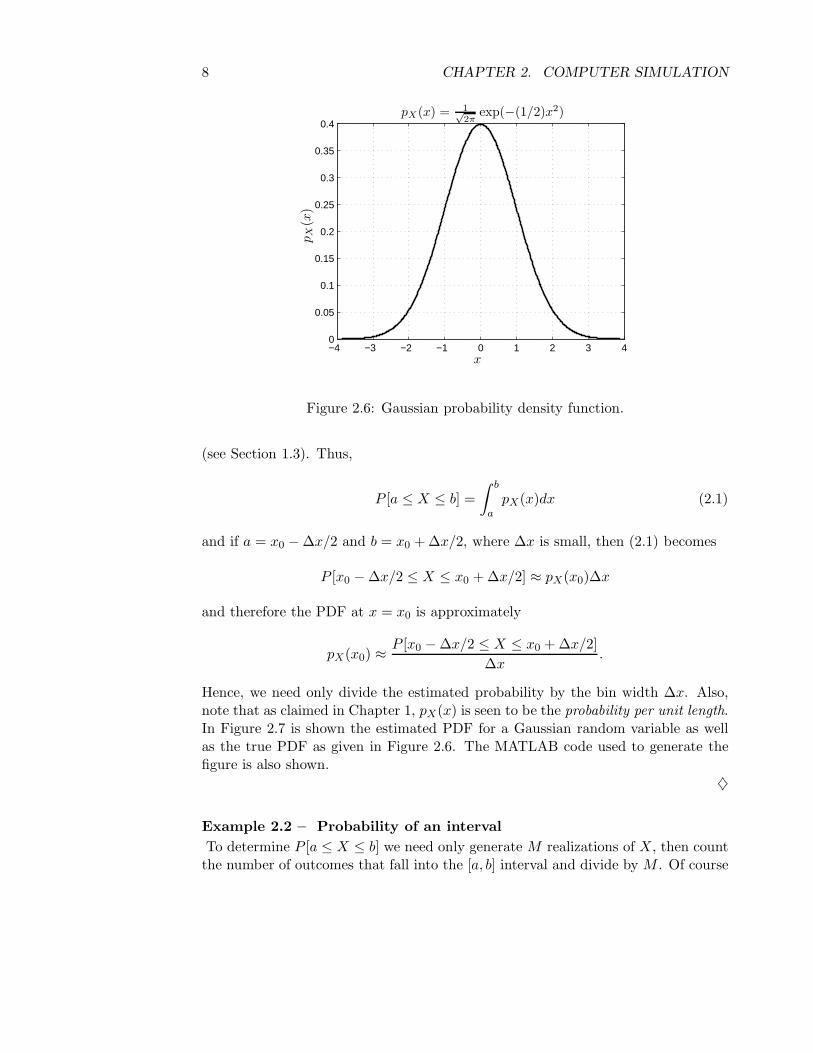
Figure 2.6: Gaussian probability density function.

(see Section 1.3). Thus,

P [a ≤ X ≤ b] =∫ b

apX(x)dx (2.1)

and if a = x0 − ∆x/2 and b = x0 + ∆x/2, where ∆x is small, then (2.1) becomes

P [x0 − ∆x/2 ≤ X ≤ x0 + ∆x/2] ≈ pX(x0)∆x

and therefore the PDF at x = x0 is approximately

pX(x0) ≈ P [x0 − ∆x/2 ≤ X ≤ x0 + ∆x/2]∆x

.

Hence, we need only divide the estimated probability by the bin width ∆x. Also,note that as claimed in Chapter 1, pX(x) is seen to be the probability per unit length.In Figure 2.7 is shown the estimated PDF for a Gaussian random variable as wellas the true PDF as given in Figure 2.6. The MATLAB code used to generate thefigure is also shown.

♦

Example 2.2 – Probability of an intervalTo determine P [a ≤ X ≤ b] we need only generate M realizations of X, then countthe number of outcomes that fall into the [a, b] interval and divide by M . Of course

2.5. DETERMINING CHARACTERISTICS OF RANDOM VARIABLES 9

−3 −2 −1 0 1 2 30

0.1

0.2

0.3

0.4

0.5

x

Est

imat

edan

dtr

ueP

DF

randn(’state’,0)x=randn(1000,1);bincenters=[-3.5:0.5:3.5]’;bins=length(bincenters);h=zeros(bins,1);for i=1:length(x)for k=1:bins

if x(i)>bincenters(k)-0.5/2 ...& x(i)<=bincenters(k)+0.5/2h(k,1)=h(k,1)+1;

endend

endpxest=h/(1000*0.5);xaxis=[-4:0.01:4]’;px=(1/sqrt(2*pi))*exp(-0.5*xaxis.^2);

Figure 2.7: Estimated and true probability density functions.

M should be large. In particular, if we let a = 2 and b = ∞, then we should obtainthe value (which must be evaluated using numerical integration)

P [X > 2] =∫ ∞

2

1√2π

exp(−(1/2)x2

)dx = 0.0228

and therefore very few realizations can be expected to fall in this interval. The resultsfor an increasing number of realizations are shown in Figure 2.8. This illustrates theproblem with the simulation of small probability events. It requires a large numberof realizations to obtain accurate results. (See Problem 11.47 on how to reduce thenumber of realizations required.)

♦

Example 2.3 – Average valueIt is frequently important to measure characteristics of X in addition to the PDF.For example, we might only be interested in the average or mean or expected valueof X. If the random variable is Gaussian, then from Figure 2.6 we would expect Xto be zero on the average. This conjecture is easily “verified” by using the samplemean estimate

1M

M∑i=1

xi

10 CHAPTER 2. COMPUTER SIMULATION

M Estimated P [X > 2] True P [X > 2]100 0.0100 0.02281000 0.0150 0.0228

10,000 0.0244 0.0288100,000 0.0231 0.0288

randn(’state’,0)M=100;count=0;x=randn(M,1);for i=1:M

if x(i)>2count=count+1;

endendprobest=count/M

Figure 2.8: Estimated and true probabilities.

of the mean. The results are shown in Figure 2.9.

M Estimated mean True mean100 0.0479 01000 −0.0431 0

10,000 0.0011 0100,000 0.0032 0

randn(’state’,0)M=100;meanest=0;x=randn(M,1);for i=1:Mmeanest=meanest+(1/M)*x(i);

endmeanest

Figure 2.9: Estimated and true mean.

♦

Example 2.4 – A transformed random variableOne of the most important problems in probability is to determine the PDF for

a transformed random variable, i.e., one that is a function of X, say X2 as anexample. This is easily accomplished by modifying the code in Figure 2.7 fromx=randn(1000,1) to x=randn(1000,1);x=x.^2;. The results are shown in Figure2.10. Note that the shape of the PDF is completely different than the originalGaussian shape (see Example 10.7 for the true PDF). Additionally, we can obtainthe mean of X2 by using

1M

M∑i=1

x2i

2.5. DETERMINING CHARACTERISTICS OF RANDOM VARIABLES 11

−3 −2 −1 0 1 2 30

0.2

0.4

0.6

0.8

x2

Est

imat

edP

DF

Figure 2.10: Estimated PDF of X2 for X Gaussian.

as we did in Example 2.3. The results are shown in Figure 2.11.

M Estimated mean True mean100 0.7491 11000 0.8911 1

10,000 1.0022 1100,000 1.0073 1

randn(’state’,0)M=100;meanest=0;x=randn(M,1);for i=1:M

meanest=meanest+(1/M)*x(i)^2;endmeanest

Figure 2.11: Estimated and true mean.

♦

Example 2.5 – Multiple random variablesConsider an experiment that yields two random variables or the vector random

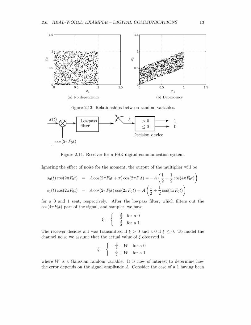
variable [X1 X2]T , where T denotes the transpose. An example might be the choiceof a point in the square {(x, y) : 0 ≤ x ≤ 1, 0 ≤ y ≤ 1} according to some procedure.This procedure may or may not cause the value of x2 to depend on the value ofx1. For example, if the result of many repetitions of this experiment produced aneven distribution of points indicated by the shaded region in Figure 2.12a, then wewould say that there is no dependency between X1 and X2. On the other hand, ifthe points were evenly distributed within the shaded region shown in Figure 2.12b,then there is a strong dependency. This is because if, for example, x1 = 0.5, thenx2 would have to lie in the interval [0.25, 0.75]. Consider next the random vector

12 CHAPTER 2. COMPUTER SIMULATION

0 0.5 1 1.50

0.5

1

1.5

x1

x2

(a) No dependency

0 0.5 1 1.50

0.5

1

1.5

x1

x2

(b) Dependency

Figure 2.12: Relationships between random variables.

[X1

X2

]=

[U1

U2

]

where each Ui is generated using rand. The result of M = 1000 realizations is shownin Figure 2.13a. We say that the random variables X1 and X2 are independent. Ofcourse, this is what we expect from a good random number generator. If instead,we defined the new random variables,

[X1

X2

]=

[U1

12U1 + 1

2U2

]

then from the plot shown in Figure 2.13b, we would say that the random variablesare dependent. Note that this type of plot is called a scatter diagram.

♦

2.6 Real-World Example – Digital Communications

In a phase-shift keyed (PSK) digital communication system a binary digit (alsotermed a bit), which is either a “0” or a “1”, is communicated to a receiver bysending either s0(t) = A cos(2πF0t + π) to represent a “0” or s1(t) = A cos(2πF0t)to represent a “1”, where A > 0 [Proakis 1989]. The receiver that is used to decodethe transmission is shown in Figure 2.14. The input to the receiver is the noise

corrupted signal or x(t) = si(t) + w(t), where w(t) represents the channel noise.

2.6. REAL-WORLD EXAMPLE – DIGITAL COMMUNICATIONS 13

0 0.5 1 1.50

0.5

1

1.5

x1

x2

(a) No dependency

0 0.5 1 1.50

0.5

1

1.5

x1

x2

(b) Dependency

Figure 2.13: Relationships between random variables.

Lowpassfilter

x(t)

cos(2πF0t)

ξ

Decision device

01> 0

≤ 0

Figure 2.14: Receiver for a PSK digital communication system.

Ignoring the effect of noise for the moment, the output of the multiplier will be

s0(t) cos(2πF0t) = A cos(2πF0t + π) cos(2πF0t) = −A

(12

+12

cos(4πF0t))

s1(t) cos(2πF0t) = A cos(2πF0t) cos(2πF0t) = A

(12

+12

cos(4πF0t))

for a 0 and 1 sent, respectively. After the lowpass filter, which filters out thecos(4πF0t) part of the signal, and sampler, we have

ξ =

{−A

2 for a 0A2 for a 1.

The receiver decides a 1 was transmitted if ξ > 0 and a 0 if ξ ≤ 0. To model thechannel noise we assume that the actual value of ξ observed is

ξ =

{−A

2 + W for a 0A2 + W for a 1

where W is a Gaussian random variable. It is now of interest to determine howthe error depends on the signal amplitude A. Consider the case of a 1 having been

14 CHAPTER 2. COMPUTER SIMULATION

transmitted. Intuitively, if A is a large positive amplitude, then the chance that thenoise will cause an error or equivalently, ξ ≤ 0, should be small. This probability,termed the probability of error and denoted by Pe, is given by P [A/2 + W ≤ 0].Using a computer simulation we can plot Pe versus A with the result shown in Figure2.15. Also, the true Pe is shown. (In Example 10.3 we will see how to analyticallydetermine this probability.) As expected, the probability of error decreases as the

0 1 2 3 4 50

0.05

0.1

0.15

0.2

0.25

0.3

0.35

0.4

0.45

0.5

A

Pe

Simulated PeTrue Pe

Figure 2.15: Probability of error for a PSK communication system.

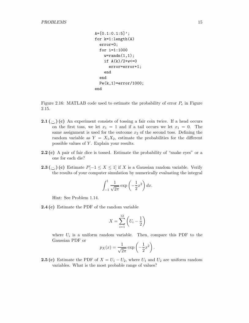
signal amplitude increases. With this information we can design our system bychoosing A to satisfy a given probability of error requirement. In actual systemsthis requirement is usually about Pe = 10−7. Simulating this small probabilitywould be exceedingly difficult due to the large number of trials required (but seealso Problem 11.47). The MATLAB code used for the simulation is given in Figure2.16.

References

Proakis, J., Digitial Communications, Second Ed., McGraw-Hill, New York, 1989.

Problems

Note: All the following problems require the use of a computer simulation. Arealization of a uniform random variable is obtained by using rand(1,1) while arealization of a Gaussian random variable is obtained by using randn(1,1).

PROBLEMS 15

A=[0.1:0.1:5]’;for k=1:length(A)

error=0;for i=1:1000w=randn(1,1);if A(k)/2+w<=0

error=error+1;end

endPe(k,1)=error/1000;

end

Figure 2.16: MATLAB code used to estimate the probability of error Pe in Figure2.15.

2.1 (�. . ) (c) An experiment consists of tossing a fair coin twice. If a head occurson the first toss, we let x1 = 1 and if a tail occurs we let x1 = 0. Thesame assignment is used for the outcome x2 of the second toss. Defining therandom variable as Y = X1X2, estimate the probabilities for the differentpossible values of Y . Explain your results.

2.2 (c) A pair of fair dice is tossed. Estimate the probability of “snake eyes” or aone for each die?

2.3 (�. . ) (c) Estimate P [−1 ≤ X ≤ 1] if X is a Gaussian random variable. Verifythe results of your computer simulation by numerically evaluating the integral∫ 1

−1

1√2π

exp(−1

2x2

)dx.

Hint: See Problem 1.14.

2.4 (c) Estimate the PDF of the random variable

X =12∑i=1

(Ui − 1

2

)

where Ui is a uniform random variable. Then, compare this PDF to theGaussian PDF or

pX(x) =1√2π

exp(−1

2x2

).

2.5 (c) Estimate the PDF of X = U1 − U2, where U1 and U2 are uniform randomvariables. What is the most probable range of values?

16 CHAPTER 2. COMPUTER SIMULATION

2.6 (�. . ) (c) Estimate the PDF of X = U1U2, where U1 and U2 are uniform randomvariables. What is the most probable range of values?

2.7 (c) Generate realizations of a discrete random variable X, which takes on values1, 2, and 3 with probabilities p1 = 0.1, p2 = 0.2 and p3 = 0.7, respectively.Next based on the generated realizations estimate the probabilities of obtainingthe various values of X.

2.8 (�. . ) (c) Estimate the mean of U , where U is a uniform random variable. Whatis the true value?

2.9 (c) Estimate the mean of X +1, where X is a Gaussian random variable. Whatis the true value?

2.10 (c) Estimate the mean of X2, where X is a Gaussian random variable.

2.11 (�. . ) (c) Estimate the mean of 2U , where U is a uniform random variable.

What is the true value?

2.12 (c) It is conjectured that if X1 and X2 are Gaussian random variables, thenby subtracting them (let Y = X1 − X2), the probable range of values shouldbe smaller. Is this true?

2.13 (�. . ) (c) A large circular dartboard is set up with a “bullseye” at the center of

the circle, which is at the coordinate (0, 0). A dart is thrown at the center butlands at (X,Y ), where X and Y are two different Gaussian random variables.What is the average distance of the dart from the bullseye?

2.14 (�. . ) (c) It is conjectured that the mean of

√U , where U is a uniform random

variable, is√

mean of U . Is this true?

2.15 (c) The Gaussian random variables X1 and X2 are linearly transformed to thenew random variables

Y1 = X1 + 0.1X2

Y2 = X1 + 0.2X2.

Plot a scatter diagram for Y1 and Y2. Could you approximately determine thevalue of Y2 if you knew that Y1 = 1?

2.16 (c,w) Generate a scatter diagram for the linearly transformed random vari-ables

X1 = U1

X2 = U1 + U2

PROBLEMS 17

where U1 and U2 are uniform random variables. Can you explain why thescatter diagram looks like a parallelogram? Hint: Define the vectors

X =

[X1

X2

]

e1 =

[1

1

]

e2 =

[0

1

]

and express X as a linear combination of e1 and e2.

18 CHAPTER 2. COMPUTER SIMULATION

Appendix 2A

Brief Introduction to MATLAB

A brief introduction to the scientific software package MATLAB is contained in thisappendix. Further information is available at the web site www.mathworks.com.MATLAB is a scientific computation and data presentation language.

Overview of MATLAB

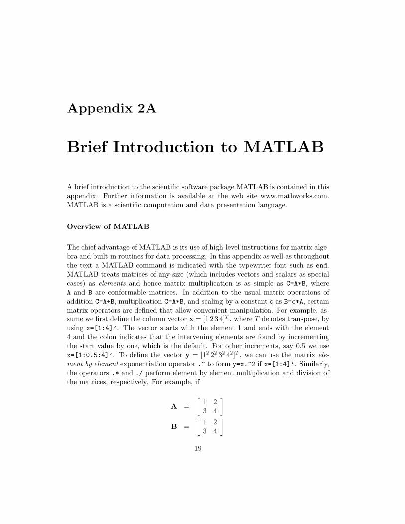
The chief advantage of MATLAB is its use of high-level instructions for matrix alge-bra and built-in routines for data processing. In this appendix as well as throughoutthe text a MATLAB command is indicated with the typewriter font such as end.MATLAB treats matrices of any size (which includes vectors and scalars as specialcases) as elements and hence matrix multiplication is as simple as C=A*B, whereA and B are conformable matrices. In addition to the usual matrix operations ofaddition C=A+B, multiplication C=A*B, and scaling by a constant c as B=c*A, certainmatrix operators are defined that allow convenient manipulation. For example, as-sume we first define the column vector x = [1 2 3 4]T , where T denotes transpose, byusing x=[1:4]’. The vector starts with the element 1 and ends with the element4 and the colon indicates that the intervening elements are found by incrementingthe start value by one, which is the default. For other increments, say 0.5 we usex=[1:0.5:4]’. To define the vector y = [12 22 32 42]T , we can use the matrix ele-ment by element exponentiation operator .^ to form y=x.^2 if x=[1:4]’. Similarly,the operators .* and ./ perform element by element multiplication and division ofthe matrices, respectively. For example, if

A =[

1 23 4

]

B =[

1 23 4

]

19

20 CHAPTER 2. COMPUTER SIMULATION

Character Meaning+ addition (scalars, vectors, matrices)- subtraction (scalars, vectors, matrices)* multiplication (scalars, vectors, matrices)/ division (scalars)^ exponentiation (scalars, square matrices).* element by element multiplication./ element by element division.^ element by element exponentiation; suppress printed output of operation: specify intervening values’ conjugate transpose (transpose for real vectors, matrices)... line continuation (when command must be split)% remainder of line interpreted as comment== logical equals| logical or& logical and~ = logical not

Table 2A.1: Definition of common MATLAB characters.

then the statements C=A.*B and D=A./B produce the results

C =[

1 49 16

]

D =[

1 11 1

]

respectively. A listing of some common characters is given in Table 2A.1. MATLABhas the usual built-in functions of cos, sin, etc. for the trigonometric functions,sqrt for a square root, exp for the exponential function, and abs for absolute value,as well as many others. When a function is applied to a matrix, the function isapplied to each element of the matrix. Other built-in symbols and functions andtheir meanings are given in Table 2A.2.

Matrices and vectors are easily specified. For example, to define the columnvector c1 = [1 2]T , just use c1=[1 2].’ or equivalently c1=[1;2]. To define the Cmatrix given previously, the construction C=[1 4;9 16] is used. Or we could firstdefine c2 = [4 16]T by c2=[4 16].’ and then use C=[c1 c2]. It is also possibleto extract portions of matrices to yield smaller matrices or vectors. For example,to extract the first column from the matrix C use c1=C(:,1). The colon indicatesthat all elements in the first column should be extracted. Many other convenientmanipulations of matrices and vectors are possible.

APPENDIX 2A. BRIEF INTRODUCTION TO MATLAB 21

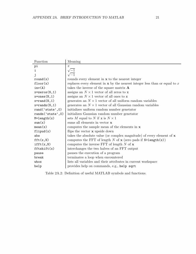
Function Meaningpi πi

√−1j

√−1round(x) rounds every element in x to the nearest integerfloor(x) replaces every element in x by the nearest integer less than or equal to xinv(A) takes the inverse of the square matrix Ax=zeros(N,1) assigns an N × 1 vector of all zeros to xx=ones(N,1) assigns an N × 1 vector of all ones to xx=rand(N,1) generates an N × 1 vector of all uniform random variablesx=randn(N,1) generates an N × 1 vector of all Gaussian random variablesrand(’state’,0) initializes uniform random number genetatorrandn(’state’,0) initializes Gaussian random number genetatorM=length(x) sets M equal to N if x is N × 1sum(x) sums all elements in vector xmean(x) computes the sample mean of the elements in xflipud(x) flips the vector x upside downabs takes the absolute value (or complex magnitude) of every element of xfft(x,N) computes the FFT of length N of x (zero pads if N>length(x))ifft(x,N) computes the inverse FFT of length N of xfftshift(x) interchanges the two halves of an FFT outputpause pauses the execution of a programbreak terminates a loop when encounteredwhos lists all variables and their attributes in current workspacehelp provides help on commands, e.g., help sqrt

Table 2A.2: Definition of useful MATLAB symbols and functions.

22 CHAPTER 2. COMPUTER SIMULATION

Any vector that is generated whose dimensions are not explicitly specified isassumed to be a row vector. For example, if we say x=ones(10), then it will bedesignated as the 1× 10 row vector consisting of all ones. To yield a column vectoruse x=ones(10,1).

Loops are implemented with the construction

for k=1:10x(k,1)=1;

end

which is equivalent to x=ones(10,1). Logical flow can be accomplished with theconstruction

if x>0y=sqrt(x);

elsey=0;

end

Finally, a good practice is to begin each program or script, which is called an “m”file (due to its syntax, for example, pdf.m), with a clear all command. Thiswill clear all variables in the workspace since otherwise, the current program mayinadvertently (on the part of the programmer) use previously stored variable data.

Plotting in MATLAB

Plotting in MATLAB is illustrated in the next section by example. Some usefulfunctions are summarized in Table 2A.3.

Function Meaningfigure opens up a new figure windowplot(x,y) plots the elements of x versus the elements of yplot(x1,y1,x2,y2) same as above except multiple plots are madeplot(x,y,’.’) same as plot except the points are not connectedtitle(’my plot’) puts a title on the plotxlabel(’x’) labels the x axisylabel(’y’) labels the y axisgrid draws grid on the plotaxis([0 1 2 4]) plots only the points in range 0 ≤ x ≤ 1 and 2 ≤ y ≤ 4text(1,1,’curve 1’) places the text “curve 1” at the point (1,1)hold on holds current plothold off releases current plot

Table 2A.3: Definition of useful MATLAB plotting functions.

APPENDIX 2A. BRIEF INTRODUCTION TO MATLAB 23

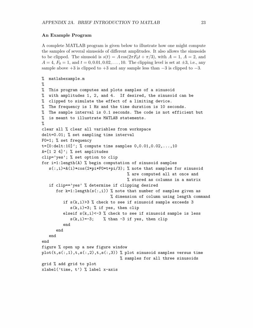
An Example Program

A complete MATLAB program is given below to illustrate how one might computethe samples of several sinusoids of different amplitudes. It also allows the sinusoidsto be clipped. The sinusoid is s(t) = A cos(2πF0t + π/3), with A = 1, A = 2, andA = 4, F0 = 1, and t = 0, 0.01, 0.02, . . . , 10. The clipping level is set at ±3, i.e., anysample above +3 is clipped to +3 and any sample less than −3 is clipped to −3.

% matlabexample.m%% This program computes and plots samples of a sinusoid% with amplitudes 1, 2, and 4. If desired, the sinusoid can be% clipped to simulate the effect of a limiting device.% The frequency is 1 Hz and the time duration is 10 seconds.% The sample interval is 0.1 seconds. The code is not efficient but% is meant to illustrate MATLAB statements.%clear all % clear all variables from workspacedelt=0.01; % set sampling time intervalF0=1; % set frequencyt=[0:delt:10]’; % compute time samples 0,0.01,0.02,...,10A=[1 2 4]’; % set amplitudesclip=’yes’; % set option to clipfor i=1:length(A) % begin computation of sinusoid samples

s(:,i)=A(i)*cos(2*pi*F0*t+pi/3); % note that samples for sinusoid% are computed all at once and% stored as columns in a matrix

if clip==’yes’ % determine if clipping desiredfor k=1:length(s(:,i)) % note that number of samples given as

% dimension of column using length commandif s(k,i)>3 % check to see if sinusoid sample exceeds 3

s(k,i)=3; % if yes, then clipelseif s(k,i)<-3 % check to see if sinusoid sample is less

s(k,i)=-3; % than -3 if yes, then clipend

endend

endfigure % open up a new figure windowplot(t,s(:,1),t,s(:,2),t,s(:,3)) % plot sinusoid samples versus time

% samples for all three sinusoidsgrid % add grid to plotxlabel(’time, t’) % label x-axis

24 CHAPTER 2. COMPUTER SIMULATION

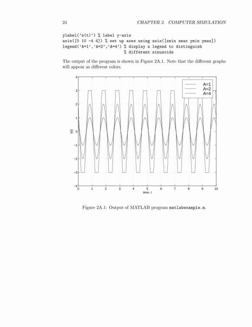
ylabel(’s(t)’) % label y-axisaxis([0 10 -4 4]) % set up axes using axis([xmin xmax ymin ymax])legend(’A=1’,’A=2’,’A=4’) % display a legend to distinguish

% different sinusoids

The output of the program is shown in Figure 2A.1. Note that the different graphswill appear as different colors.

0 1 2 3 4 5 6 7 8 9 10−4

−3

−2

−1

0

1

2

3

4

time, t

s(t)

A=1A=2A=4

Figure 2A.1: Output of MATLAB program matlabexample.m.