Du

Ma

b

a

ARRAA

KOSPPNMDDM

1

s2a[cpatcacegse

m

h1

Applied Soft Computing 52 (2017) 247–261

Contents lists available at ScienceDirect

Applied Soft Computing

j ourna l h o mepage: www.elsev ier .com/ locate /asoc

etection and sizing of metal-loss defects in oil and gas pipelinessing pattern-adapted wavelets and machine learning

ohamed Layounia,b,∗, Mohamed Salah Hamdia, Sofiène Taharb

Ahmed Bin Mohammed Military College, P.O. Box 22713, Doha, QatarConcordia University, Electrical & Computer Engineering Department, 1455 de Maisonneuve Blvd. W, Montreal, Quebec, Canada H3G 1M8

r t i c l e i n f o

rticle history:eceived 7 May 2014eceived in revised form 26 October 2016ccepted 27 October 2016vailable online 8 November 2016

eywords:il and gas pipelinesafety assessment

a b s t r a c t

Signals collected from the magnetic scans of metal-loss defects have distinct patterns. Experiencedpipeline engineers are able to recognize those patterns in magnetic flux leakage (MFL) scans ofpipelines, and use them to characterize defect types (e.g., corrosion, cracks, dents, etc.) and esti-mate their lengths and depths. This task, however, can be highly cumbersome to a human operator,because of the large amount of data to be analyzed. This paper proposes a solution to automatethe analysis of MFL signals. The proposed solution uses pattern-adapted wavelets to detect and esti-mate the length of metal-loss defects. Once the parts of MFL signals corresponding to metal-lossdefects are isolated, artificial neural networks are used to predict their depth. The proposed technique

attern-adapted waveletsattern recognitioneural networksachine learningefect locationefect sizingagnetic flux leakage

is computationally efficient, achieves high levels of accuracy, and works for a wide range of defectshapes.

© 2016 Elsevier B.V. All rights reserved.

. Introduction

Oil and gas pipelines are an important component of the energyector nowadays. In the US, 70% of all petroleum transported in009 was carried by pipeline [4]. In Canada, 97% of all natural gasnd crude oil production is currently being transported by pipeline14]. However, despite being considered as one of the safest andheapest ways to transport oil and gas [13,14], pipelines are stillrone to a variety of metal-loss defects such as corrosion, cracks,nd dents. These defects are mainly due to factors, such as extremeemperature and pressure inside the pipeline, exposure to highlyorrosive chemicals, water, etc. The repercussions of not detectingnd repairing such defects on time can be very serious: huge finan-ial losses, damage to the environment, health and life hazards,tc. Given the size of an average pipeline, and the amount of data

enerated from magnetic scans, relying on human operators toift through the data and find defects is a highly challenging andrror-prone task.

∗ Corresponding author. Tel.: (+1) 514 848 2424.E-mail addresses: layouni@ece.concordia.ca (M. Layouni),

shamdi@abmmc.edu.qa (M.S. Hamdi), tahar@ece.concordia.ca (S. Tahar).

ttp://dx.doi.org/10.1016/j.asoc.2016.10.040568-4946/© 2016 Elsevier B.V. All rights reserved.

This paper describes a solution to automate the process ofinspecting MFL data [16–18] generated through the scanning of oiland gas pipelines. The proposed solution uses a technique basedon pattern-adapted wavelets [15,36] to detect, locate, and estimatethe length of metal loss defects along the pipeline. Once a defectis located, a number of features are extracted from the corre-sponding MFL signal. Those features are then fed into an artificialneural network which returns an estimate of the defect depth. Theobtained depth and length are then used to assign a severity ratingto the detected defect, and decide whether or not urgent repairsare due. The severity rating is assigned using industry standardssuch as ASME.BG31 [3], which provides a formula to evaluate adefect’s severity given its dimensions, the operating pressure insidethe pipeline, and other properties of the steel used to build thepipeline.

Related work. The development of techniques to assess thesafety of oil and gas pipelines has attracted the attention of manyresearchers over the last several years [17,18,46,41,51,20,39,50].Results on this topic are very diverse in terms of what they achieve,

the specific problems they address, and the approaches they use.Fig. 1 provides a high-level summary of the research landscapein this area. Following the notation in Fig. 1, we can divide theliterature on this topic into three main groups:

248 M. Layouni et al. / Applied Soft Computing 52 (2017) 247–261

ork a

GG

G

aotIntp

lw

wwTltt

B

wttsDn

Fig. 1. Summary of related w

roup I. Numerical techniques to determine defect sizes.roup II. Non-numerical techniques to detect and locate defects

(sizing problem not considered).roup III. Non-numerical techniques to detect, locate, and deter-

mine the opening length of defects. Some of the work inthis category does also provide ways to classify defectsand other pipeline features into different types (e.g., holes,valves, junctions, etc.).

It is worth noting at this point that work listed under Groups IInd III includes cases where the application domain is not related toil and gas pipelines. Some of the techniques, for example, relate tohe detection and location of defects in underground power cables.n some cases also, the signals being analyzed are not MFL sig-als (e.g., electrical, acoustic, and pressure wave signals). None ofhe non-numerical methods found in the literature considered theroblem of determining defect depths.

In the following, we summarize each of the group of techniquesisted above, and show the similarities and differences with the

ork in this paper.Group I: Numerical techniques to determine defect sizes. The

ork in [17,18,46] considered numerical methods, not based onavelets, to address the problem of defect sizing from MFL signals.

hese methods however only apply to defect shapes for which ana-ytical models are known. The approach proposed in [17,18,46] iso express the relationship between MFL signals and defect geome-ries through an equation of the form:

MFL = F(D) (1)

here BMFL denotes the MFL signals, D denotes the defect geome-ry, and F(·) denotes the analytical model describing the behavior of

he MFL signals in relation to the defect geometry. Determining theize of a defect, then, reduces to inverting Equation (1) and finding

given BMFL and F(·). This approach is straightforward, but has aumber of limitations: (i) Eq. (1) may have several solutions, which

nd comparison to this paper.

could lead to several plausible defect geometries; (ii) solving Eq. (1)has a high computational cost – at least cubic in the size of the MFLsignals matrix BMFL [29]; and (iii) the analytical model F(·) itself isnot always available. In fact, apart from a limited number of simpledefect shapes (e.g., cylindrical, spherical, spheroidal, and cuboidal[18,46,29]), analytical models for general arbitrary defect shapesare still hard to derive [18,46]. This is due to the fact that derivinganalytical models requires solving Maxwell’s equations of mag-netism [1], which is not easy for defects of general arbitrary shapes.

The authors in [17,18,46] demonstrate their approach on a num-ber of simple defect shapes, and solve the sizing problem usingtechniques such as the finite element method (FEM) [48], linearalgebra, and machine learning. However, as explained above, it ishard to apply this approach to defects of arbitrary shapes.

More recently, the authors in [42] have used numerical methodsto study the relationship between MFL signals and defect geome-tries (length and depth). They conclude their paper by confirmingthe non-linear nature of the relationship between MFL signals anddefect geometries. They do also point out the difficulty of usingnumerical methods for determining defect depths from MFL sig-nals, since several defect geometries can lead to the same MFL signalcharacteristics (e.g., maximum peak amplitude).

Building on the observations of [42], the work in [44] usesnumerical methods to estimate the worst-case defect depth corre-sponding to a given MFL signal. The proposed method is applied toan MFL model generated from a non-linear FEM approximation. Theauthors conclude by pointing out that the accuracy of the worst-case defect depth depends on the quality of the MFL model beingused, and that for defects deeper than 70% of the wall’s thickness,the solutions found by their method may not be correct.

Finally, the work in [27] describes a model to estimate defect

depths as a quadratic function of the MFL peak values. The param-eters of the model, however, are obtained by computing an FEMapproximation of the MFL field for a given defect shape. The exper-imental results reported by the authors show that their method

ft Com

atlw

mls

sooc

tcutiputi[pp

oaotiao

mwsinnfs

psrdoafipl

steittdtorcs

The solution in this paper does not rely on analytical models, andcan detect the occurrence of any reference pattern in the MFL sig-nal. As a result, the proposed technique can handle a wide range

M. Layouni et al. / Applied So

chieves an estimation error of less than 20% of the pipeline wall’shickness, which is acceptable by industry standards. The mainimitation of [27] is that it relies on FEM-derived analytical models,

hich can be obtained only for simple defect shapes.The work presented in this paper does not require analytical

odels, and uses pattern-adapted wavelets [36,37] and machineearning techniques [22,38] that can be applied to any defecthapes.

Group II: Non-numerical techniques to detect and locate defects (noizing). The authors in [41,51] have used wavelets for the purposef de-noising MFL signals, as well as detecting, and locating defectsil and gas pipelines. The problem of defect sizing however was notonsidered by these authors.

Wavelets have also been used in other applications, includinghe detection and characterization of faults in underground powerables [31,35,25,6]. More precisely, the authors in [31,35,25,6] havesed wavelet transforms to detect and locate faults, and classifyhem into a set of predefined fault types. The work in [31,35,25,6]s related to this paper, but there are two important differences. Inarticular, the work in this paper models defects as 3D objects, andses wavelets both to locate them and determine their sizes, whilehe work in [31,35,25,6] does not consider the sizing problem, sincet models faults as discrete points on a line. Moreover, the work in31,35,25,6] uses general purpose mother wavelets, whereas thisaper uses a customized mother wavelet adapted to the referenceattern to be detected.

Wavelets [37] have also been used previously in the area of biol-gy, for example, to detect various health problems, such as brainnd heart illnesses [36,2,19]. Their usage in biology, however, wasnly to detect anomalies, and not to quantify them. In other words,he problems considered in [2,19] are mainly detection problems:.e., the goal was to analyze signals from biological measurements,nd determine which parts of the signals are normal, and whichnes are abnormal.

Group III: Non-numerical techniques to detect, locate, and deter-ine the opening length of defects. The authors in [9,39,50] have usedavelets to analyze other types of signals, namely pressure wave

ignals inside a pipeline, for the purpose of detecting and locat-ng holes and other features (e.g., valves, junctions) in a pipelineetwork. The work in [20] uses similar signal processing methods,amely, the Hilbert transform (HT) [45] and Hilbert–Huang trans-

orm (HHT) [45], to detect and locate holes from pressure waveignals.

The solutions proposed in [9,20,39,50] rely on the followinghysical phenomenon. A leaking hole causes a local change in den-ity in the fluid flowing inside the pipeline, which in turn provokeseflections in the pressure wave signal. These reflections can beetected as echoes. The techniques in [9,20,50] infer the locationf the defect from the time it takes for echoes to arrive at someppropriately placed sensor. The solutions in [9,50] use two noise-ltering techniques (Kurtosis [5] and Cepstrum [11]) to make itossible to recognize echoes in the wavelet transform, despite high

evels of noise in the pressure wave signals.The work in [39] assumes a slightly different setting, where two

ensors are placed at two different locations on the pipeline, suchhat the distance between the two is known. The pipeline is thenxcited with a pressure wave, which propagates through the fluidnside the pipeline, and produces a reflexive wave when encoun-ering a hole. The technique in [39] estimates the time difference itakes for the reflexive wave to arrive at each sensor. Given this timeifference and the wave speed, the authors in [39] infer the loca-ion of the defect. The work in [39] conducts a fine-grained analysis

f the wave speed of direct waves (non-dispersive waves) and theeflective waves (dispersive waves), thereby achieving higher pre-ision than earlier methods based on cross-correlation between theignals received at each sensor [40,8].

puting 52 (2017) 247–261 249

While related, there are some important differences betweenthe work presented in this paper and those in [9,20,39,50].

1. First, the goal of this paper is to detect not only holes and leaks,but also defects that do not lead to a hole in the pipeline wall.This includes for example, superficial metal-loss defects fromcorrosion, or construction defects inside the pipeline wall (i.e.,an air gap inside the wall of the pipeline that does not show anyfeatures on the external surface of the pipeline wall). In the caseof a superficial metal-loss (e.g., from corrosion), it is not clearif the resulting echoes in the pressure wave signals would beimportant enough to be detected. For construction defects (i.e.,air gaps inside the pipeline wall), it is clear that pressure wavesignals cannot detect their presence. These two types of defects,as well as holes, are however detectable using MFL signals. Thisis probably the reason why MFL scanning is the most widely usedinspection method in the oil and gas industry.

2. The authors in [39] indicate also that the method they propose isnot applicable to pipelines carrying incompressible fluids suchas crude oil because the used technique relies on a particularbehavior of vibro-acoustic waves in compressible fluids such asgas. The MFL signals used in this paper do not have this con-straint, and work on any type of metallic pipelines regardless ofthe fluid or gas they carry.

3. Moreover, the method proposed in this paper provides an esti-mate of the opening length and depth of a defect, and not onlyits location. By contrast, the technique in [39] is mainly intendedfor locating hole defects. However, that technique could be usedto infer the opening length of a defect, if the location of each edgeof a defect is determined.

4. The work in this paper uses wavelets for a completely differentpurpose than [9,39,50]. For instance, the work in [9,50] use thewavelet transform to filter out noise from pressure wave signals(which will be further analyzed to find “spikes” in amplitude, orechoes, whose coordinates indicate the location of holes on thepipeline). This work on the other hand uses wavelet transformsto locate the occurrence of a possibly dilated version of a refer-ence pattern in the MFL signals. Such an occurrence causes a localmaximum in the Wavelet Transform. This is possible, becausethe mother wavelet in this paper is built from the pattern signalof the defect to be detected.1 The solutions in [9,39,50] on theother hand, use generic mother wavelets (Morlet and the Mex-ican Hat), either to filter noisy signals, or to detect peaks in thewavelet transform; the latter correspond to the arrival time ofreflected echoes.

5. Finally, the work in [20] uses Hilbert transform (HT) andHilbert–Huang transform (HHT) to analyze pressure wave sig-nals. While the patterns being detected in [20] are differentfrom the ones in this paper, further research needs to be doneto see how those signal processing techniques can be appliedto MFL signals. The question of estimating defect sizes (open-ing length and depth) using the techniques in [20] needs to befurther explored as well.

Summary of paper contribution. This paper presents a tech-nique to detect and locate defects in MFL data, and determinetheir lengths and depths. The proposed technique is based onpattern-adapted wavelets [36,37] and machine learning [22,38].

of defect shapes, even those for which no analytical models are

1 More details on the use of pattern-adapted wavelets are given in Section 3.2.

250 M. Layouni et al. / Applied Soft Computing 52 (2017) 247–261

etic fl

ka

lhluttttatw

2

pmlthltcasnotmrmtMwvp

Fig. 2. Magn

nown. Unlike related work in Groups II and III, this paper presents technique to estimate defect depths from MFL signals.

Paper outline. The remainder of this paper is organized as fol-ows. Section 2 gives a brief overview on MFL scanning, andighlights the main idea behind its use in the detection of metal-

oss defects. Section 3 introduces wavelets and shows how they aresed to locate defects and estimate their length. Section 4 describeshe features extracted from the MFL signals of detected defects, andhe artificial neural network built to analyze them. It also presentshe performance results and compares them to those achieved byhe linear regressions technique. Section 6 provides a summary,nd discusses the performance of the overall solution. Finally, Sec-ion 7 provides concluding remarks and ideas for extending thisork.

. MFL-based pipeline inspection

MFL scanning is a well established technique for inspectingipelines made from ferromagnetic material [3]. The techniqueakes it possible to detect, locate, and estimate the size of metal

oss defects present on a pipeline. The idea behind MFL scanning ishe following. When two strong magnets of opposite polarity areeld close to the surface of a pipeline, the latter is magnetized, and

ines of magnetic force flow through the walls of the pipeline, fromhe south pole to the north pole. When the pipeline wall contains arack or a thinning (due to corrosion, for example), two new polesppear at the edges of the crack: a north pole and a south pole,imilar to when a magnet is broken in two. As a result, the mag-etic lines of force now flow through the ferromagnetic materialf the pipeline wall, then through the air gap created by the crack,hen again through the ferromagnetic material (Fig. 2a). The set of

agnetic lines of force flowing through these materials (e.g., fer-omagnetic steel, air) is called magnetic flux. And the density ofagnetic flux in each material depends on a physical property of

he material called Magnetic Permeability. Informally speaking, the

agnetic Permeability of a given material denotes the degree tohich magnetic flux is able to flow through that material. This is

ery similar to the concept of conductivity in electricity, or fluidermeability in porous materials such as rocks.

Fig. 3. MFL measure

ux leakage.

Different materials have different magnetic permeability. Forinstance, ferromagnetic steel has a much higher magnetic per-meability than air. Therefore, the density of magnetic flux in thehealthy parts of the pipeline is much higher than the density ofmagnetic flux in the air gap created by the crack (Fig. 2b). As aresult, the magnetic lines of force bulge out as they go throughthe air gap, because air cannot absorb as much flux per unit vol-ume as the ferromagnetic material of the pipeline. This bulgingof magnetic flux is called Magnetic Flux Leakage; it is the physi-cal phenomenon the pipeline industry relies on to detect defects inoil and gas pipelines. Fig. 2a illustrates the magnetic flux leakagephenomenon.

In MFL-based inspection, a scanning tool equipped with strongmagnets and magnetic sensors is sent inside a pipeline. The wallsof the pipeline are magnetized, and sensors are used to measureany magnetic flux leakage. The sensors are equally-distributedaround the circumference of the pipeline, and move with theinspection tool parallel to the axis of the pipeline. The use ofseveral sensors around the circumference of the pipeline makesit possible to precisely locate the angular position of a defect.Fig. 3 shows a rolled-out representation of the pipeline, and howthe MFL sensors are equally spaced along the x-axis, above thepipeline. Any magnetic flux leakage detected by the sensors indi-cates the presence of a defect. The MFL signals measured bythe sensors are recorded, and later analyzed to locate possibledefects, and determine their sizes and severity levels. MFL sig-nals are the main input data to the solution presented in thispaper.

3. Pattern-adapted wavelets for the detection and sizing ofmetal-loss defects

3.1. MFL signal patterns around defect edges

MFL signals recorded in the neighborhood of a metal-loss defect

have a distinct shape. Figs. 4 and 5 show sample MFL signalssimulated for cylindrical and cuboidal defects, respectively. Fig. 5displays the individual MFL signals simulated for each of the sen-sors passing above the defect. The X and Y axes in Figs. 4 and 5, as

ment setting.

M. Layouni et al. / Applied Soft Computing 52 (2017) 247–261 251

(top) a

wai

ctat

Fig. 4. MFL scan of cylindrical

ell as the sensors trajectories and direction of magnetization, ares indicated in Fig. 3. The MFL signals in Figs. 4 and 5 were simulatedn MATLAB [34] using analytical models described in [16–18,29].

As can be seen in Fig. 4, the sensor passing directly above theenter of the defect (i.e., along x = 0) has the MFL signal for whichhe axial and radial components have the highest amplitude. This

mplitude gets lower for sensors further away from the center ofhe defect. The MFL signals of other regularly-shaped defects (such

Fig. 5. MFL signals from each of the s

nd cuboidal (bottom) defects.

as spheroidal and spherical defects) have patterns similar to theones in Figs. 4 and 5.

As can be noted in Figs. 4 and 5, MFL signals show a distinctbehavior around defect edges. For example, peaks in the tangen-tial and radial components (Bx and Bz) of the MFL signal mark thelocation of defect edges. The technique proposed in this paper uses

the MFL behavior around metal-loss defects as a reference pattern.The next subsection explains how this reference pattern is used in

ensors passing above a defect.

252 M. Layouni et al. / Applied Soft Computing 52 (2017) 247–261

th thr

cl

3

e[strto

m

w

s

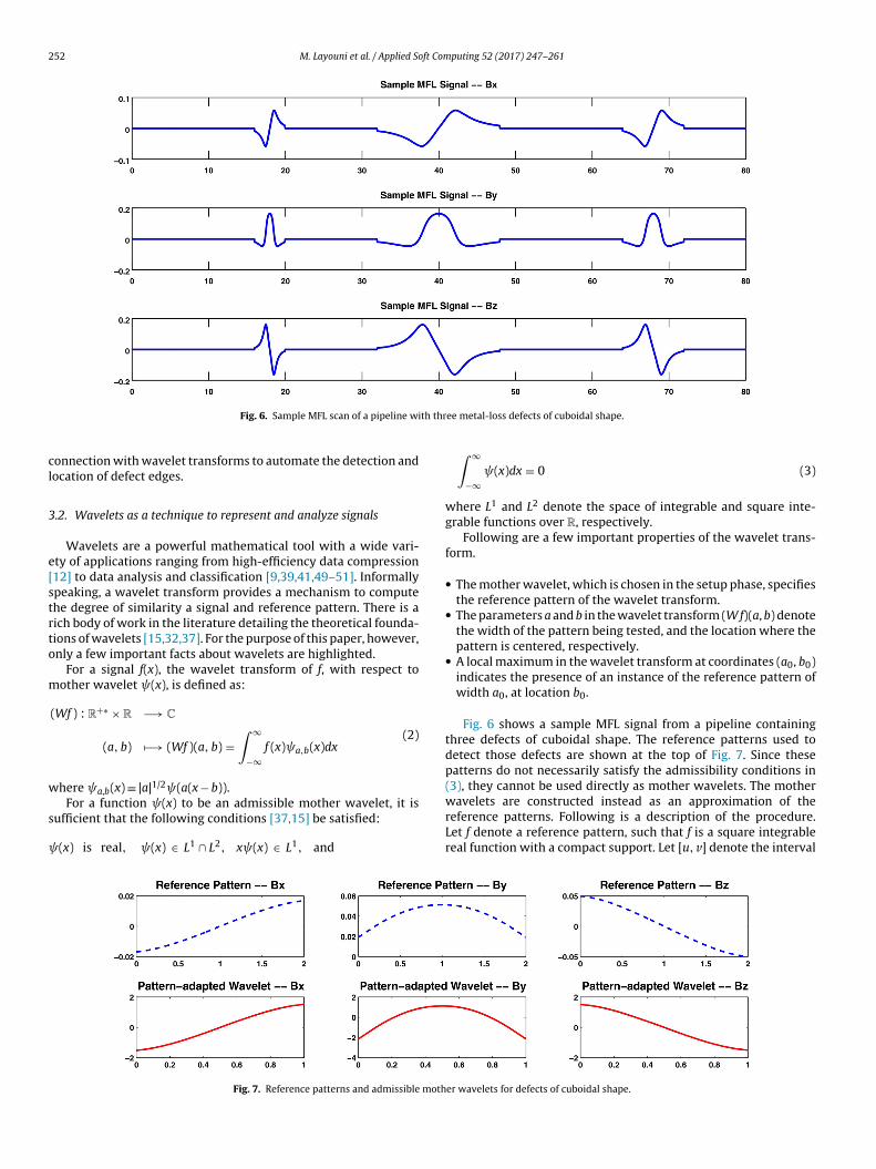
Fig. 6. Sample MFL scan of a pipeline wi

onnection with wavelet transforms to automate the detection andocation of defect edges.

.2. Wavelets as a technique to represent and analyze signals

Wavelets are a powerful mathematical tool with a wide vari-ty of applications ranging from high-efficiency data compression12] to data analysis and classification [9,39,41,49–51]. Informallypeaking, a wavelet transform provides a mechanism to computehe degree of similarity a signal and reference pattern. There is aich body of work in the literature detailing the theoretical founda-ions of wavelets [15,32,37]. For the purpose of this paper, however,nly a few important facts about wavelets are highlighted.

For a signal f(x), the wavelet transform of f, with respect toother wavelet (x), is defined as:

(Wf ) : R+∗ × R −→ C

(a, b) �−→ (Wf )(a, b) =∫ ∞

−∞f (x) a,b(x)dx

(2)

here a,b(x) ≡ |a|1/2 (a(x − b)).

For a function (x) to be an admissible mother wavelet, it is

ufficient that the following conditions [37,15] be satisfied:

(x) is real, (x) ∈ L1 ∩ L2, x (x) ∈ L1, and

Fig. 7. Reference patterns and admissible moth

ee metal-loss defects of cuboidal shape.

∫ ∞

−∞ (x)dx = 0 (3)

where L1 and L2 denote the space of integrable and square inte-grable functions over R, respectively.

Following are a few important properties of the wavelet trans-form.

• The mother wavelet, which is chosen in the setup phase, specifiesthe reference pattern of the wavelet transform.

• The parameters a and b in the wavelet transform (W f)(a, b) denotethe width of the pattern being tested, and the location where thepattern is centered, respectively.

• A local maximum in the wavelet transform at coordinates (a0, b0)indicates the presence of an instance of the reference pattern ofwidth a0, at location b0.

Fig. 6 shows a sample MFL signal from a pipeline containingthree defects of cuboidal shape. The reference patterns used todetect those defects are shown at the top of Fig. 7. Since thesepatterns do not necessarily satisfy the admissibility conditions in(3), they cannot be used directly as mother wavelets. The mother

wavelets are constructed instead as an approximation of thereference patterns. Following is a description of the procedure.Let f denote a reference pattern, such that f is a square integrablereal function with a compact support. Let [u, v] denote the interval

er wavelets for defects of cuboidal shape.

M. Layouni et al. / Applied Soft Computing 52 (2017) 247–261 253

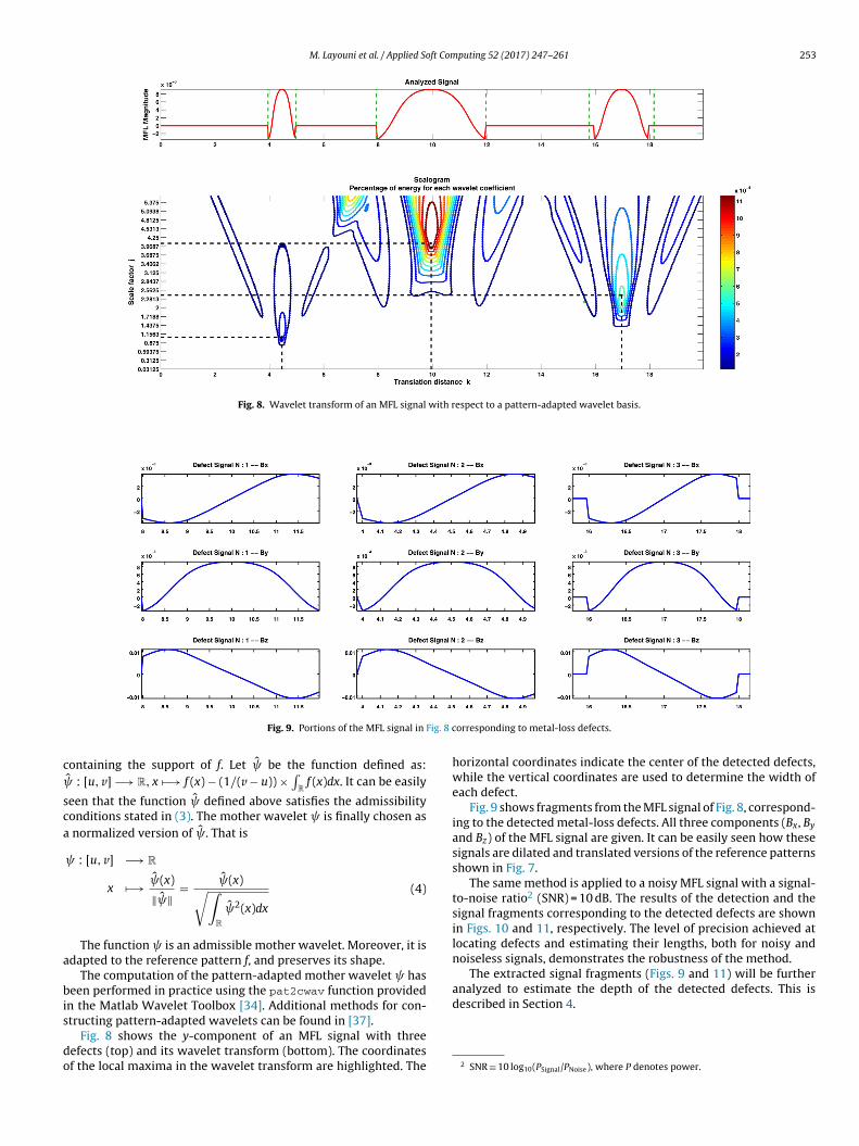
Fig. 8. Wavelet transform of an MFL signal with respect to a pattern-adapted wavelet basis.

Fig. 8 c

c

sca

a

bis

do

analyzed to estimate the depth of the detected defects. This isdescribed in Section 4.

Fig. 9. Portions of the MFL signal in

ontaining the support of f. Let be the function defined as:ˆ : [u, v] −→ R, x �−→ f (x) − (1/(v − u)) ×

∫Rf (x)dx. It can be easily

een that the function defined above satisfies the admissibilityonditions stated in (3). The mother wavelet is finally chosen as

normalized version of . That is

: [u, v] −→ R

x �−→ (x)

‖ ‖= (x)√∫

R

2(x)dx

(4)

The function is an admissible mother wavelet. Moreover, it isdapted to the reference pattern f, and preserves its shape.

The computation of the pattern-adapted mother wavelet haseen performed in practice using the pat2cwav function provided

n the Matlab Wavelet Toolbox [34]. Additional methods for con-

tructing pattern-adapted wavelets can be found in [37].

Fig. 8 shows the y-component of an MFL signal with threeefects (top) and its wavelet transform (bottom). The coordinatesf the local maxima in the wavelet transform are highlighted. The

orresponding to metal-loss defects.

horizontal coordinates indicate the center of the detected defects,while the vertical coordinates are used to determine the width ofeach defect.

Fig. 9 shows fragments from the MFL signal of Fig. 8, correspond-ing to the detected metal-loss defects. All three components (Bx, By

and Bz) of the MFL signal are given. It can be easily seen how thesesignals are dilated and translated versions of the reference patternsshown in Fig. 7.

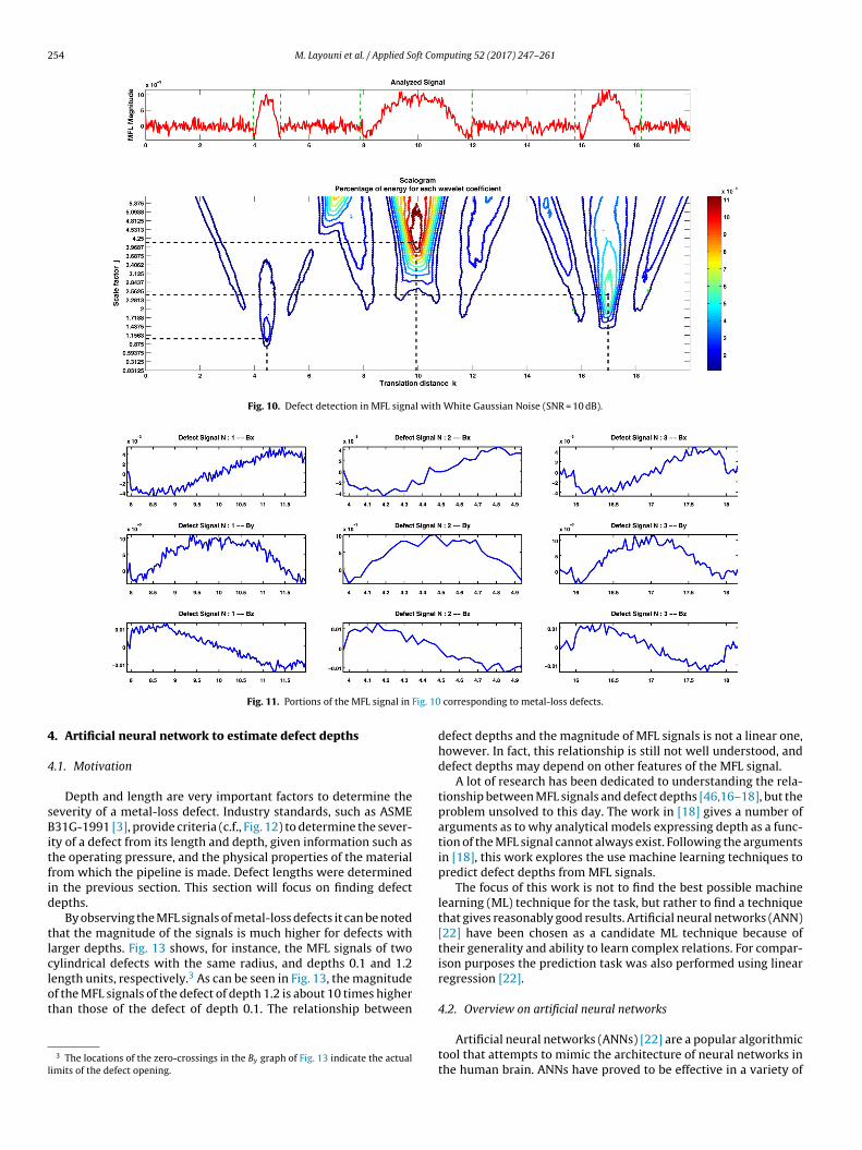
The same method is applied to a noisy MFL signal with a signal-to-noise ratio2 (SNR) = 10 dB. The results of the detection and thesignal fragments corresponding to the detected defects are shownin Figs. 10 and 11, respectively. The level of precision achieved atlocating defects and estimating their lengths, both for noisy andnoiseless signals, demonstrates the robustness of the method.

The extracted signal fragments (Figs. 9 and 11) will be further

2 SNR ≡ 10 log10(PSignal/PNoise), where P denotes power.

254 M. Layouni et al. / Applied Soft Computing 52 (2017) 247–261

Fig. 10. Defect detection in MFL signal with White Gaussian Noise (SNR = 10 dB).

Fig. 10

4

4

sBitfid

tlclot

l

Fig. 11. Portions of the MFL signal in

. Artificial neural network to estimate defect depths

.1. Motivation

Depth and length are very important factors to determine theeverity of a metal-loss defect. Industry standards, such as ASME31G-1991 [3], provide criteria (c.f., Fig. 12) to determine the sever-

ty of a defect from its length and depth, given information such ashe operating pressure, and the physical properties of the materialrom which the pipeline is made. Defect lengths were determinedn the previous section. This section will focus on finding defectepths.

By observing the MFL signals of metal-loss defects it can be notedhat the magnitude of the signals is much higher for defects witharger depths. Fig. 13 shows, for instance, the MFL signals of twoylindrical defects with the same radius, and depths 0.1 and 1.2

ength units, respectively.3 As can be seen in Fig. 13, the magnitudef the MFL signals of the defect of depth 1.2 is about 10 times higherhan those of the defect of depth 0.1. The relationship between

3 The locations of the zero-crossings in the By graph of Fig. 13 indicate the actualimits of the defect opening.

corresponding to metal-loss defects.

defect depths and the magnitude of MFL signals is not a linear one,however. In fact, this relationship is still not well understood, anddefect depths may depend on other features of the MFL signal.

A lot of research has been dedicated to understanding the rela-tionship between MFL signals and defect depths [46,16–18], but theproblem unsolved to this day. The work in [18] gives a number ofarguments as to why analytical models expressing depth as a func-tion of the MFL signal cannot always exist. Following the argumentsin [18], this work explores the use machine learning techniques topredict defect depths from MFL signals.

The focus of this work is not to find the best possible machinelearning (ML) technique for the task, but rather to find a techniquethat gives reasonably good results. Artificial neural networks (ANN)[22] have been chosen as a candidate ML technique because oftheir generality and ability to learn complex relations. For compar-ison purposes the prediction task was also performed using linearregression [22].

4.2. Overview on artificial neural networks

Artificial neural networks (ANNs) [22] are a popular algorithmictool that attempts to mimic the architecture of neural networks inthe human brain. ANNs have proved to be effective in a variety of

M. Layouni et al. / Applied Soft Computing 52 (2017) 247–261 255

Fig. 12. Parabolic criteria for classifying corrosion defects based on length and depth, for a given pipeline material and operating pressure [3].

drica

tdAmapoIeaTF

stwdmpwc

complete, the resulting neural network can be used to predict F onfresh input data.

ANNs have been applied in a variety of fields, ranging fromrobotics [21], to data science [10], to medicine [2,26], and financial

Fig. 13. Difference in MFL magnitude for cylin

asks such as data fitting, function approximation, time series pre-iction, data classification, data clustering, etc. Generally speaking,NNs can be thought of as a computational tool capable of approxi-ating a function having multiple inputs and outputs. It consists of

graph of neurons linked to each other by edges. Each neuron com-utes a function (called Activation function) on the values receivedn its input edges, and sends the result forward on its output edge.n addition, each neuron Ni in the network has a bias bi, and eachdge linking neuron Ni to Nj has a weight Wij. Let Ai() denote thectivation function of neuron Ni, and let Ii1, . . ., Iik denote its inputs.he output of neuron Ni is computed as Oi = Ai(bi +

∑kj=1WijIj).

ig. 14 shows an example of an artificial neural network.The network of neurons described above is augmented with a

earch algorithm that determines the optimal weights and biaseshat minimize the error between the final output of the net-ork, and the output of the function to be approximated. Let Fenote the function to be approximated. The search for the opti-

al weights and biases is an iterative process that loops through

airs of input–output data {(X�, F(X�)), � ∈ [1, M]}, and adjusts theeights and biases so that the output of the network on inputs X� is

loser to F(X�). This phase, when the network parameters are being

l defects of same radius and different depths.

adjusted, is called the training phase, and the set of pairs {(X�, F(X�)),� ∈ [1, M]} is called the training data. When the training phase is

Fig. 14. Structure of an artificial neural network.

256 M. Layouni et al. / Applied Soft Com

Table 1Number of principal components for noisy and noiseless data sets.

Noiseless SNR = 10 dB SNR = 5 dB SNR = 3 dB

Number of principalcomponents explaining95% of the variance in the

7 8 9 10

m[

4

fvta

4

aimcirk

t

•••••

tmpFdata3t[ndpl

Aie

tmpt

data

arkets forecasting [28]. More details about ANNs can be found in22].

.3. Preparing the dataset

Raw MFL signals are vectors of arbitrary sizes and cannot beed directly to the ML techniques considered in this work. Instead,arious features are first extracted from the signals and then usedo build a dataset. The next section discusses the choice of features,nd describes the feature extraction procedure.

.4. Extracting features from MFL signals

There are many possible features that can be extracted from given signal. These can range from characteristics such as max-mum magnitude and peak-to-peak distance, to metrics such as

ean-average and standard deviation. The goal, however, is toompute the smallest set of features that captures most of thenformation contained in the signal. Ideally, one should be able toegenerate the signal right from the extracted set of features, whileeeping the latter small.

In this work, the following features were extracted because ofheir apparent dependence on the defect depth.

maximum magnitude,peak-to-peak distance,mean average,standard deviation,integral of the normalized signal.4

The above features do capture a lot of the information con-ained in the signals, but not everything. To make sure, the

aximum amount of information about the signal is captured,olynomial series were used to approximate the MFL signals.or this particular instance of the MFL signals, polynomials ofegrees 3, 6, and 6 provided the best approximation for Bx, By,nd Bz respectively. By convention, a degree n polynomial is writ-en P(X) ≡ anXn + · · · + a1X + a0. The coefficients of the polynomialpproximations, along with the above features, give a total of3 features (33 = (5 × 3) + 4 +7 + 7). To reduce the number of fea-ures and remove redundancy, principal component analysis (PCA)24,23] was conducted on the data set. Table 1 gives the finalumber of features for noisy and noiseless MFL signals. The initialataset (with 33 features) is projected along the principal com-onents obtained through PCA, and the result is fed to a machine

earning algorithm.Two machine learning techniques are considered in this paper:

NN and linear regression. Non-linear parametric regression [47]s another technique that was considered. It should be noted, how-ver, that to use non-linear regression, one needs to choose a

4 The signal is first normalized with respect to the maximum magnitude, andhen normalized with respect to position. That is, the position of the two peaks are

apped to −1 and +1, and the signal is shrunk to fit on the [−1,1] interval. Thisrovides a better way to compare signals on the same interval while preservingheir overall shape.

puting 52 (2017) 247–261

parametrized non-linear model of the form Y = f(X, ˇ), where X is thepredictors matrix, Y the values to be predicted, and a parametersvector. The goal then is to find the optimal value of the parametersvector that allows f to best fit the data. There are numerous fami-lies of functions from which f can be chosen: exponential functions,logarithmic functions, trigonometric functions, nth root functions,rational functions, polynomials of various degrees, etc. The firstchallenge is to find a suitable family of functions to express f, thatwill allow it to fit the data with an acceptable level of accuracy.This is not an easy task. All the non-linear models that were triedin this work resulted in much lower accuracy than the methodsbased on ANNs and linear regression. This is due to the fact thatthe chosen models were not adequate for the data at hand. Findingthe right model is not easy, especially when many parameters areinvolved.

Neural networks on the other hand, are known for their ability tolearn non-linear relations, without requiring a model of those rela-tions as an input. The models obtained in this work, using neuralnetworks, are in fact non-linear, and their accuracy is much higherthan that of linear models. In cases where a model of the relation-ship between input and output is not known, neural networks canbe a practical alternative to non-linear prediction.

4.5. Defect depth prediction using ANNs

This work explored the use of feedforward neural networks(FFNNs) [22]. Other types of neural networks will be consideredin a future work. The dataset comprises around 1300 data items(input features and target output). Each data item correspondsto a cylindrical defect of a different size (radius and depth). Thedataset is first partitioned into three separate sets: one for training,one for cross-validation, and one for testing. The partitioning isperformed using random sampling; the indices of the set are firstshuffled through a random permutation. Then the first 70% areassigned to the training set, the next 15% to the validation set, andthe remaining 15% to the test set. The neural network is trainedusing the Early Stopping Cross-validation technique [43] whichcan be summarized in Fig. 15.

4.6. Neural network size and architecture

A number of parameters can be fine-tuned to obtain the optimalneural network configuration for the task at hand. These includeparameters such as:

1. The number of hidden layers, and the size of each layer.2. The error performance function (e.g., mean squared error, sum

squared error, etc.)3. The training algorithm (e.g., gradient descent [22,38],

Levenberg–Marquardt [30,33], etc.)4. The transfer functions [22,38] used in the hidden layer neurons

(e.g., log sigmoid, hyperbolic tangent sigmoid, etc.)

The experiments presented in this paper sought to optimize theANN with respect to the number of hidden layers and their sizes,and kept the other parameters fixed as follows:

1. Error performance function: mean squared error.2. Training algorithm: Levenberg–Marquardt.3. Transfer function: log sigmoid.

It might be useful to conduct an optimization search withrespect the parameters above, but this is not in scope for this paper.

To find the optimal network size, an experiment was performedfor ANNs with 1, 2, and 3 hidden layers, where each layer had a

M. Layouni et al. / Applied Soft Computing 52 (2017) 247–261 257

Fig. 15. ANN training using Early Stopping Cross-validation [43].

nuMpuoput

4

s(piwdTA

TO

and noiseless signals. The tables in Appendix A give the length siz-ing accuracy at 70% and 90% certainty. As Table 3 shows, the length

umber of neurons ranging from 5 to 100. Each of the ANN config-rations above was used to analyze data from noiseless and noisyFL signals with SNRs equal to 10 dB, 5 dB, and 3 dB, and the error

erformance was recorded. All experiments were done in MATLABsing the Neural Networks Toolbox [7]. The optimal network sizesbtained from those experiments are shown in Table 2. The depthrediction experiments presented in the remainder of this paperse the optimal networks sizes shown in Table 2. The results ofhose experiments are given in Section 5.3.

.7. Defect depth prediction using linear regression

For the sake of comparison, the same datasets from the previousections were used to predict defect depths using linear regressionLR) [22]. To make the comparison as precise as possible, the sameartitions (training, validation, and testing) used in the ANN exper-

ments, were also used for linear regression. The training datasetsere used to compute the linear regression models, and the testatasets to compute the error performance of the linear regression.

he results of the linear regression, as well as comparison with theNN performance are given in Section 5.3.

able 2ptimal ANN sizes and MSEs for noisy and noiseless data sets.

1 hidden layer 2 hidden layers 3 hidden layers

Noiseless [40]/4.8e−05 [25,5]/8.3e−06 [45,5,25]/4.7e−06SNR = 10 dB [65]/0.0271 [15,5]/0.0181 [25,65,5]/0.0165SNR = 5 dB [85]/0.0285 [15,25]/0.0253 [45,45,5]/0.0271SNR = 3 dB [45]/0.0175 [45,35]/0.0172 [5,65,25]/0.0170

5. Performance results

5.1. Performance criterion

The performance criterion adopted in this paper is PredictionAccuracy @80% Certainty, which is defined as the half width of theerror interval that the prediction method can guarantee for at least80% of the test dataset. For example, a prediction accuracy @80%of ±10% means that the prediction error, for at least 80% of thedataset, is in the range ±10% of the real defect depth. Accuracy athigher or lower levels of certainty (e.g., @95% or @70%) can alsobe considered, depending on the sensitivity of the application. Thiscriterion is used to evaluate the accuracy of defect length and defectdepth predictions.

5.2. Performance results of defect length prediction

Table 3 shows the accuracy @80% certainty of defect length pre-dictions based on the WT technique. The accuracy is given for noisy

sizing accuracy of the WT-based technique is almost perfect fornoiseless signals, but decreases for noisy signals. To improve the

Table 3Length prediction accuracy @80% certainty.

Length accuracy @80% certainty

WT alone WT + LR WT + 1-lay. ANN WT + 2-lay. ANN

Noiseless ±2% ±2% ±1% ±2%SNR = 10 dB ±7% ±4% ±3% ±2%SNR = 5 dB ±20% ±7% ±5% ±5%SNR = 3 dB ±39% ±16% ±8% ±11%

258 M. Layouni et al. / Applied Soft Computing 52 (2017) 247–261

Table 4Depth prediction accuracy @80% certainty.

Depth accuracy @80% certainty

2-Layer ANN 3-Layer ANN Linear regression

Noiseless <±1% <±1% ±25%SNR = 10 dB ±10% ±9% ±35%SNR = 5 dB ±13% ±14% ±40%

ldfaSWt1da

iwipim

5

lttt

ooflaS

Table 5Best accuracy results achieved.

Accuracy @80% certainty

Length prediction Depth accuracy

Noiseless ±1% <±1%SNR = 10 dB ±2% ±9%

SNR = 3 dB ±11% ±12% ±26%

ength sizing accuracy for noisy signals, the defect lengths pre-icted by the WT technique were combined with features extractedrom defect signals, and fed to machine learning techniques (ANNsnd linear regression). More precisely, the features extracted inection 4.4 were added to the defect lengths predicted by theavelet-based technique of Section 3.2. PCA was then applied to

he dataset, thereby reducing the number of features from 34 to 7 or0 depending on the noise level (c.f., Table 1). The projection of theataset along the principal components was then fed to one-layernd two-layer ANNs, as well as linear regression.

As can be seen in Table 3, the application of machine learn-ng techniques has drastically improved the length sizing accuracy,

ith the WT + 1-layer ANN combination giving the best results. Its worth noting here that applying the ML techniques to the WT-redicted defect lengths alone did not lead to any improvement

n accuracy. Adding the extracted features produced the improve-ents shown in Table 3.

.3. Performance results of defect depth prediction

Table 4 shows the accuracy @80% achieved by two-hidden-ayer and three-hidden-layer ANNs, as well as the linear regressionechnique. All accuracy figures in Table 4 were computed on theest Dataset. The network sizes used for the two-hidden-layer andhree-hidden-layer ANNs are the optimal ones, indicated in Table 2.

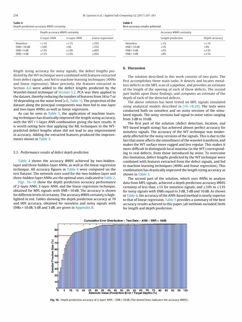
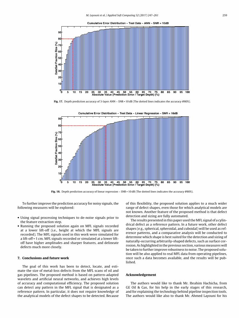
Figs. 16–18 show the depth prediction accuracy performancef 2-layer ANN, 3-layer ANN, and the linear regression technique,btained for MFL signals with SNR = 10 dB. The accuracy is shownor different levels of certainty. The accuracy @80% certainty is high-ighted in red. Tables showing the depth prediction accuracy at 70

nd 90% accuracy, obtained for noiseless and noisy signals withNRs = 10 dB, 5 dB and 3 dB, are given in Appendix B.

Fig. 16. Depth prediction accuracy of 2-layer ANN – SNR = 1

SNR = 5 dB ±5% ±13%SNR = 3 dB ±8% ±11%

6. Discussion

The solution described in this work consists of two parts. Thefirst accomplishes three main tasks. It detects and locates metal-loss defects in the MFL scan of a pipeline, and provides an estimateof the length of the opening of each of those defects. The secondpart builds upon those findings, and computes an estimate of thedepth of each of the detected defects.

The above solution has been tested on MFL signals simulatedusing analytical models described in [16–18,29]. The tests wereconducted both on noiseless and on noisy versions of the simu-lated signals. The noisy versions had signal to noise ratios rangingfrom 3 dB to 10 dB.

The first part of the solution (defect detection, location, andWT-based length sizing) has achieved almost perfect accuracy fornoiseless signals. The accuracy of the WT technique was moder-ately affected for the noisy versions of the signals. This is due to thefact that noise affects the smoothness of the wavelet transform, andmakes the WT surface more rugged and less regular. This makes itmore difficult to distinguish local maxima (in the WT) correspond-ing to real defects, from those introduced by noise. To overcomethis limitation, defect lengths predicted by the WT technique werecombined with features extracted from the defect signals, and fedto machine learning techniques (ANNs and linear regression). Thiscombination has drastically improved the length sizing accuracy asshown in Table 3.

The second part of the solution, which uses ANNs to analyzedata from MFL signals, achieved a depth prediction accuracy @80%certainty of less than ±1% for noiseless signals, and ±10% to ±13%for noisy signals with SNRs equal to 3 dB, 5 dB and 10 dB. As shownin Table 4, the accuracy of the ANN-based method is neatly superior

to that of linear regression. Table 5 provides a summary of the bestaccuracy results achieved in this paper (all methods included) bothfor length and depth prediction.

0 dB (The dotted lines indicates the accuracy @80%).

M. Layouni et al. / Applied Soft Computing 52 (2017) 247–261 259

Fig. 17. Depth prediction accuracy of 3-layer ANN – SNR = 10 dB (The dotted lines indicates the accuracy @80%).

– SNR

f

•

•

7

mgwocrt

Fig. 18. Depth prediction accuracy of linear regression

To further improve the prediction accuracy for noisy signals, theollowing measures will be explored:

Using signal processing techniques to de-noise signals prior tothe feature extraction step.Running the proposed solution again on MFL signals recordedat a lower lift-off (i.e., height at which the MFL signals arerecorded). The MFL signals used in this work were simulated fora lift-off = 1 cm. MFL signals recorded or simulated at a lower lift-off have higher amplitudes and sharper features, and delineatedefects much more closely.

. Conclusions and future work

The goal of this work has been to detect, locate, and esti-ate the size of metal-loss defects from the MFL scans of oil and

as pipelines. The proposed method is based on pattern-adaptedavelets and artificial neural networks, and achieves high levels

f accuracy and computational efficiency. The proposed solutionan detect any pattern in the MFL signal that is designated as aeference pattern. In particular, it does not require knowledge ofhe analytical models of the defect shapes to be detected. Because

= 10 dB (The dotted lines indicates the accuracy @80%).

of this flexibility, the proposed solution applies to a much widerrange of defect shapes, even those for which analytical models arenot known. Another feature of the proposed method is that defectdetection and sizing are fully automated.

The results presented in this paper used the MFL signal of a cylin-drical defect as a reference pattern. In a future work, other defectshapes (e.g., spherical, spheroidal, and cuboidal) will be used as ref-erence patterns, and a comparative analysis will be conducted todetermine which shape is best suited for the detection and sizing ofnaturally-occurring arbitrarily-shaped defects, such as surface cor-rosion. As highlighted in the previous section, various measures willbe taken to further improve robustness to noise. The proposed solu-tion will be also applied to real MFL data from operating pipelines,once such a data becomes available, and the results will be pub-lished.

Acknowledgement

The authors would like to thank Mr. Ibrahim Hachicha, fromGE Oil & Gas, for his help in the early stages of this research,and for explaining the technology behind pipeline inspection tools.The authors would like also to thank Mr. Ahmed Layouni for his

2 ft Com

hw

fdo

A

TL

TL

A

TD

TD

R

[

[

[

[

[

[

[

[

[

[

[

[

[[

[

[

[

[

[

[

[

[

[[

[[

[

60 M. Layouni et al. / Applied So

elp designing an efficient algorithm to search for local maxima inavelet transform matrices.

This work was made possible by NPRP grant # [5-813-1-134]rom the Qatar National Research Fund (a member of Qatar Foun-ation). The statements made herein are solely the responsibilityf the authors.

ppendix A. Length prediction accuracy performance

able A.6ength prediction accuracy @70% certainty.

Length accuracy @70% certainty

WT alone WT + LR WT + 1-lay. ANN WT + 2-lay. ANN

Noiseless <±2% <±2% <±1% ±1%SNR = 10 dB ±6% ±3% ±3% ±2.5%SNR = 5 dB ±12% ±5% ±3.5% ±4.5%SNR = 3 dB ±21% ±11% ±6.5% ±8%

able A.7ength prediction accuracy @90% certainty.

Length accuracy @90% certainty

WT alone WT + LR WT + 1-lay. ANN WT + 2-lay. ANN

Noiseless ±8% ±5% ±3.5% ±2.5%SNR = 10 dB ±12% ±5% ±5% ±5%SNR = 5 dB ±40% ±10% ±7% ±9%SNR = 3 dB ±65% ±22% ±11% ±15%

ppendix B. Depth prediction accuracy performance

able B.8epth prediction accuracy @70%.

Depth accuracy @70% certainty

2-Layer ANN 3-Layer ANN Linear regression

Noiseless <±1% <±1% ±18%SNR = 10 dB ±7.5% ±7.5% ±26%SNR = 5 dB ±10% ±10% ±28%SNR = 3 dB ±9% ±8.5% ±20%

able B.9epth prediction accuracy @90%.

Depth accuracy @90% certainty

2-Layer ANN 3-Layer ANN Linear regression

Noiseless ±2.5% <±1% ±56%SNR = 10 dB ±20% ±21% ±66%SNR = 5 dB ±22% ±24% ±90%SNR = 3 dB ±16% ±19% ±46%

eferences

[1] A. Aharoni, Introduction to the Theory of Ferromagnetism, Oxford UniversityPress, 1996.

[2] A. Al-Fahoum, I. Howitt, Combined wavelet transformation and radial basisneural networks for classifying life-threatening cardiac arrhythmias, Med.Biol. Eng. Comput. 37 (5) (1999) 566–573.

[3] American Society of Mechanical Engineers, ASME B31G – 1991 – Manual forDetermining Remaining Strength of Corroded Pipelines, 1991, Retrieved April2014: http://www.engineeringtoolbox.com/asme-d 7.html.

[4] Association of Oil Pipe Lines, Report on Shifts in Petroleum Transportation:1990–2009, 2012, Retrieved April 2014: http://www.aopl.org.

[

[

puting 52 (2017) 247–261

[5] K.P. Balanda, H. MacGillivray, Kurtosis: a critical review, Am. Stat. 42 (2)(1988) 111–119.

[6] S.H.S. Barakat, Fault Detection, Classification, and Location in UndergroundCables (Ph.D. thesis), Fayoum University, Egypt, 2014.

[7] M.H. Beale, M.T. Hag, H.B. Demuth, MATLAB Neural Network ToolboxTM –User’s Guide, MathWorks, 2014.

[8] S. Beck, M. Curren, N. Sims, R. Stanway, Pipeline network features and leakdetection by cross-correlation analysis of reflected waves, J. Hydraul. Eng. 131(8) (2005) 715–723.

[9] S. Beck, J. Foong, W. Staszewski, Wavelet and cepstrum analyses of leaks inpipe networks, in: Progress in Industrial Mathematics, vol. 8 of Mathematicsin Industry, Springer, 2006, pp. 559–563.

10] J.P. Bigus, Data Mining with Neural Networks: Solving Business Problemsfrom Application Development to Decision Support, McGraw-Hill, Inc.,1996.

11] B.P. Bogert, M.J. Healy, J.W. Tukey, Quefrency analysis of time series forechoes: cepstrum, pseudo-autocovariance, cross-cepstrum and saphecracking, in: Proceedings of the Symposium on Time Series Analysis, vol. 15,1963, pp. 209–243.

12] J.N. Bradley, C.M. Brislawn, T. Hopper, FBI wavelet/scalar quantizationstandard for gray-scale fingerprint image compression, in: SPIE Proceedings,Visual Information Processing II, vol. 1961, SPIE, 1993, pp. 293–304.

13] Canadian Energy Pipeline Association, Protecting Pipeline Integrity – It is aFull-Time Job!, 2012, Retrieved April 2014: http://www.cepa.com/2012/09.

14] Canadian Energy Pipeline Association, Facts About the Use of Energy Pipelinesin Canada, 2013, Retrieved April 2014: http://www.cepa.com/library/factoids.

15] I. Daubechies, Ten Lectures on Wavelets, Society for Industrial and AppliedMathematics, SIAM, 1992.

16] S. Dutta, F. Ghorbel, R. Stanley, Dipole modeling of magnetic flux leakage, IEEETrans. Magn. 45 (4) (2009) 1959–1965.

17] S. Dutta, F. Ghorbel, R. Stanley, Simulation and analysis of 3-D magnetic fluxleakage, IEEE Trans. Magn. 45 (4) (2009) 1966–1972.

18] S.M. Dutta, Magnetic Flux Leakage Sensing: The Forward and InverseProblems (Ph.D. thesis), Rice University, USA, 2008.

19] M. Ermes, Methods for the Classification of Biosignals Applied to theDetection of Epileptiform Waveforms and to the Recognition of PhysicalActivity (Ph.D. thesis), Tampere University of Technology, Finland, 2009.

20] M. Ghazali, W.J. Staszewski, J. Shucksmith, J.B. Boxall, S.B. Beck, Instantaneousphase and frequency for the detection of leaks and features in a pipelinesystem, Struct. Health Monit. 10 (4) (2011) 351–360.

21] R. Glasius, A. Komoda, S.C. Gielen, Neural network dynamics for path planningand obstacle avoidance, Neural Netw. 8 (1) (1995) 125–133.

22] S.O. Haykin, Neural Networks and Learning Machines, Prentice Hall, 2008.23] J.E. Jackson, A User’s Guide to Principal Components. Wiley Series in

Probability and Statistics, John Wiley & Sons, Inc., 2004.24] I.T. Jolliffe, Principal Component Analysis. Springer Series in Statistics,

Springer, 2002.25] S. Kaitwanidvilai, C. Pothisarn, C. Jettanasen, P. Chiradeja, A. Ngaopitakkul,

Discrete wavelet transform and back-propagation neural networks algorithmfor fault classification in underground cable, in: Proceedings of theInternational Multiconference of Engineers and Computer Scientists, vol. II,2011, pp. 996–1000.

26] J. Khan, J.S. Wei, M. Ringner, L.H. Saal, M. Ladanyi, F. Westermann, F. Berthold,M. Schwab, C.R. Antonescu, C. Peterson, et al., Classification and diagnosticprediction of cancers using gene expression profiling and artificial neuralnetworks, Nat. Med. 7 (6) (2001) 673–679.

27] H.M. Kim, D.W. Jeong, S.H. Im, J.H. Park, J.S. Lee, G.S. Park, A study on theestimation of defect depth in MFL type NDT system, in: Proceedings of the20th International Conference on the Computation of Electromagnetic Fields(COMPUMAG), 2015, p. PA6-8.

28] N. Kohzadi, M.S. Boyd, B. Kermanshahi, I. Kaastra, A comparison of artificialneural network and time series models for forecasting commodity prices,Neurocomputing 10 (2) (1996) 169–181, Financial Applications, Part I.

29] M. Layouni, S. Tahar, M.S. Hamdi, A survey on the application of neuralnetworks in the safety assessment of oil and gas pipelines, in: IEEESymposium on Computational Intelligence for Engineering Solutions (CIES),2014, pp. 95–102.

30] K. Levenberg, A method for the solution of certain problems in least squares,Q. Appl. Math. 2 (1944) 164–168.

31] X. Ma, C. Zhou, I. Kemp, Interpretation of wavelet analysis and its applicationin partial discharge detection, IEEE Trans. Dielectr. Electr. Insul. 9 (3) (2002)446–457.

32] S. Mallat, A Wavelet Tour of Signal Processing, Academic Press, 2008.33] D.W. Marquardt, An Algorithm for Least-Squares Estimation of Nonlinear

Parameters, SIAM J. Appl. Math. 11 (2) (1963) 431–441.34] MATLAB, Version 7.12.0 (R2011a), The MathWorks Inc., 2011.35] J.C.H. Mejia, Characterization of Real Power Cable Defects by Diagnostic

Measurements (Ph.D. thesis), Georgia Institute of Technology, USA, 2008.36] H. Mesa, Adapted wavelets for pattern detection, in: Progress in Pattern

Recognition, Image Analysis and Applications, vol. 3773 of Lecture Notes inComputer Science, Springer-Verlag, 2005, pp. 933–944.

37] M. Misiti, Y. Misiti, G. Oppenheim, J.-M. Poggi, Wavelets and TheirApplications, Wiley-ISTE, 2007.

38] G. Montavon, G. Orr, K.-R. Müller, Neural Networks: Tricks of the Trade, Vol.7700 of Lecture Notes in Computer Science – Computer State-of-the-ArtSurveys, Springer, 2012.

ft Com

[

[

[

[

[

[

[[

[

[

[

[detection in gas pipelines using wavelet-based filtering, Struct. Health Monit.

M. Layouni et al. / Applied So

39] Y.-S. Moon, S.-K. Lee, Gas leakage in buried gas pipe based on wavelet analysisfor vibro-coustic signal in a long duct, J. Intell. Mater. Syst. Struct. 22 (5)(2011) 387–399.

40] J. Muggleton, M. Brennan, Leak noise propagation and attenuation insubmerged plastic water pipes, J. Sound Vibr. 278 (3) (2004) 527–537.

41] S. Mukhopadhyay, G. Srivastava, Characterisation of metal loss defects frommagnetic flux leakage signals with discrete wavelet transform, NDT&E Int. 33(1) (2000) 57–65.

42] N.R. Pearson, M.A. Boat, R.H. Priewald, M.J. Pate, J.S. Mason, A study of MFLsignals from a spectrum of defect geometries, in: Proceedings of the 18thWorld Conference on Nondestructive Testing, 2012, pp. 1546–1553.

43] L. Prechelt, Automatic early stopping using cross validation: quantifying the

criteria, Neural Netw. 11 (4) (1998) 761–767.

44] R.H. Priewald, P.D. Ledger, N.R. Pearson, J.S. Mason, Uncertainties of MFLsignal inversion and worst-case defect depth estimation using a numericalmodel, in: Electromagnetic Nondestructive Evaluation (XVI), vol. 38 of Studiesin Applied Electromagnetics and Mechanics, 2014, pp. 55–65.

[

puting 52 (2017) 247–261 261

45] R.B. Randall, Frequency Analysis, Brül & Kjor, 1987.46] M. Ravan, R. Amineh, S. Koziel, N. Nikolova, J. Reilly, Sizing of 3-D arbitrary

defects using magnetic flux leakage measurements, IEEE Trans. Magn. 46 (4)(2010) 1024–1033.

47] G. Seber, A. Lee, Linear Regression Analysis. Wiley Series in Probability andStatistics, Wiley, 2012.

48] G. Strang, G.J. Fix, An Analysis of the Finite Element Method. Prentice-HallSeries in Automatic Computation, Wellesley-Cambridge, 2008.

49] M. Unser, A. Aldroubi, A review of wavelets in biomedical applications, Proc.IEEE 84 (4) (1996) 626–638.

50] J. Urbanek, T. Barszcz, T. Uhl, W. Staszewski, S. Beck, B. Schmidt, Leak

11 (4) (2012) 405–412.51] Z. Zhang, D. Fan, Y. Sun, Fault detection in sub-sea pipelines using discrete

wavelet transform method, in: Proceedings of the Twentieth InternationalOffshore and Polar Engineering Conference, 2010, pp. 109–114.