SC I ENCE ADVANCES | R E S EARCH ART I C L E

APPL I ED SC I ENCES AND ENG INEER ING

1Thoraxcenter–Biomedical Engineering, Erasmus Medical Center, 3000 CA Rotterdam,Netherlands. 2Faculty of Applied Sciences–Imaging Physics, Delft University of Tech-nology, 2600 AA Delft, Netherlands. 3Faculty of Electrical Engineering, Mathematicsand Computer Science–Micro Electronics, Delft University of Technology, 2628 CDDelft, Netherlands. 4Department of Experimental Medical Instruments, Erasmus Med-ical Center, 3015 CN Rotterdam, Netherlands.*Corresponding author. Email: p.kruizinga@erasmusmc.nl

Kruizinga et al., Sci. Adv. 2017;3 : e1701423 8 December 2017

Copyright © 2017

The Authors, some

rights reserved;

exclusive licensee

American Association

for the Advancement

of Science. No claim to

original U.S. Government

Works. Distributed

under a Creative

Commons Attribution

NonCommercial

License 4.0 (CC BY-NC).

Compressive 3D ultrasound imaging using asingle sensorPieter Kruizinga,1,2* Pim van der Meulen,3 Andrejs Fedjajevs,3 Frits Mastik,1 Geert Springeling,4

Nico de Jong,1,2 Johannes G. Bosch,1 Geert Leus3

Three-dimensional ultrasound is a powerful imaging technique, but it requires thousands of sensors andcomplex hardware. Very recently, the discovery of compressive sensing has shown that the signal structurecan be exploited to reduce the burden posed by traditional sensing requirements. In this spirit, we have designeda simple ultrasound imaging device that can perform three-dimensional imaging using just a single ultrasoundsensor. Our devicemakes a compressedmeasurement of the spatial ultrasound field using a plastic aperturemaskplaced in front of the ultrasound sensor. The aperture mask ensures that every pixel in the image is uniquelyidentifiable in the compressed measurement. We demonstrate that this device can successfully image twostructured objects placed in water. The need for just one sensor instead of thousands paves the way for cheaper,faster, simpler, and smaller sensing devices and possible new clinical applications.

Do

on July 17, 2018http://advances.sciencem

ag.org/w

nloaded from

INTRODUCTIONUltrasound imaging is a widely used technique in medical decision-making, mainly due to the fact that ultrasound devices use nonionizingradiation and are relatively low-cost. By carefully aiming the transducer,the operator can use ultrasound to obtain real-time images of specificcross sections of the body. The contrast in ultrasound images is dueto sound speed and density differences between tissues. This is why,for example, a baby’s skull in a watery womb forms a clear picture inultrasound imaging. Almost all ultrasound images aremade with trans-ducers composed of many tiny sensors (between 64 and 10,000) thatcan transmit short ultrasonic bursts (typically 1 to 40 MHz). Thesebursts are then reflected by the tissue and recorded by the same sensorarray. The time delay between transmission of the burst and detectionof the echoes defines where the tissue is located. The strength of thereflected echo contains information on the density of the tissue.

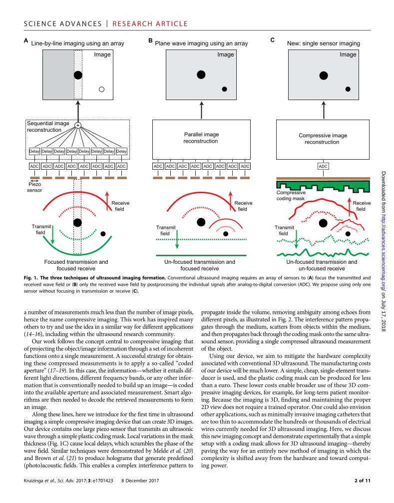
The sensors that make up these arrays are made mainly frompiezoelectric crystals. When a voltage is applied to the material, thecrystal vibrates and produces a short ultrasonic burst of a few cycles(1).When the sensors are activated with appropriate delays, the emittedultrasound wave travels along a straight line (in the form of a narrowbeam) and can be focused on a point of interest. With these focusedbeams, a whole volume can be scanned (Fig. 1A). In terms of receivingthe signal reception, similar delays can be used to selectively enhancethe signals from scatterers along the beam of interest. This type offocusing that uses delayed signals in transmitting and/or receivingis named beamforming and has been a source of active academic re-search for many years (2). One advantage of applying beamformingin receive mode is that it can be carried out digitally after the receivedultrasound field has been recorded (Fig. 1B). An alternative techniqueapplied in ultrasound imaging is to use an unfocused (“plane”) waveduring transmission. The focus is then regained upon reception,allowing for a faster frame rate because the medium is not “scanned”line by line with a focused beam.

The majority of ultrasound imaging is performed using transducerarrays that have their sensors distributed along one dimension (Fig. 1, Aand B), thereby offering a two-dimensional (2D) cross-sectional viewof the inside of the human body. To obtain a full 3D view, one needs tomechanically move or rotate the 1D array or to create a 2D array thatallows beam steering in two directions. These 2D arrays have beenshown to produce stunning high-resolution 3D images, for example,of faces of fetuses (3, 4). However, 3D ultrasound imaging is a longway from achieving the popularity of 2D ultrasound imaging apartfrom in certain medical disciplines, such as obstetrics, cardiology, andimage-guided intervention. This is surprising given that a full 3D viewshould in almost all cases allow for a better assessment of the specificmedical question. One of the main reasons for this low acceptance of3D ultrasound imaging is that 3D imaging requires a high hardwarecomplexity (>1000 sensors on a small footprint, integrated electronics,high data rates, etc.). Most of this is necessary to cope with the con-straints imposed by the Nyquist theorem when sampling the receivedradiofrequency ultrasound signals.

Fortunately, as shown by recent discoveries in statistics (5–7), theclassical idea that digitization of analog signals (such as ultrasoundwaves) demands uniform sampling at rates twice as high as the highestfrequency present (known as the Nyquist theorem) is no longer a rulecarved in stone. This discovery has opened up a very active field ofresearch known as compressive sensing (CS) (8). One of the leadingthoughts in CS is that signals generally contain some natural structure.This structure can be exploited to compress the signal to one that ismany times smaller than the original, as is done, for example, in jpegcompression of images. However, until recently, this size reductionwas always done after the signal had been acquired at full Nyquist rate.CS now allows the compression to bemerged with the sensing. As animmediate consequence, the number of measurements required to re-cover the signal of interest can be drastically reduced, potentially leadingto cheaper, faster, simpler, and smaller sensing devices. In the case ofultrasound imaging, this has already led to the development of success-ful new strategies for sampling and image reconstruction (9–12).

One of themost striking implementations of CS has been the designof the single-pixel camera by Duarte et al. (13). Here, the authors man-aged to reconstruct images using an adjustablemirrormask and a singlephotodetector. By projecting the image onto the photodetector usingrandommask patterns, they were able to recover the actual image from

1 of 11

SC I ENCE ADVANCES | R E S EARCH ART I C L E

on July 17, 2018http://advances.sciencem

ag.org/D

ownloaded from

a number of measurements much less than the number of image pixels,hence the name compressive imaging. This work has inspired manyothers to try and use the idea in a similar way for different applications(14–16), including within the ultrasound research community.

Our work follows the concept central to compressive imaging: thatof projecting the object/image information through a set of incoherentfunctions onto a single measurement. A successful strategy for obtain-ing these compressed measurements is to apply a so-called “codedaperture” (17–19). In this case, the information—whether it entails dif-ferent light directions, different frequency bands, or any other infor-mation that is conventionally needed to build up an image—is codedinto the available aperture and associated measurement. Smart algo-rithms are then needed to decode the retrieved measurements to forman image.

Along these lines, here we introduce for the first time in ultrasoundimaging a simple compressive imaging device that can create 3D images.Our device contains one large piezo sensor that transmits an ultrasonicwave through a simple plastic codingmask. Local variations in themaskthickness (Fig. 1C) cause local delays, which scrambles the phase of thewave field. Similar techniques were demonstrated by Melde et al. (20)and Brown et al. (21) to produce holograms that generate predefined(photo)acoustic fields. This enables a complex interference pattern to

Kruizinga et al., Sci. Adv. 2017;3 : e1701423 8 December 2017

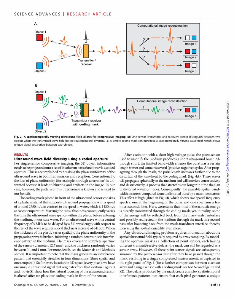
propagate inside the volume, removing ambiguity among echoes fromdifferent pixels, as illustrated in Fig. 2. The interference pattern propa-gates through the medium, scatters from objects within the medium,and then propagates back through the codingmask onto the same ultra-sound sensor, providing a single compressed ultrasound measurementof the object.

Using our device, we aim to mitigate the hardware complexityassociated with conventional 3D ultrasound. Themanufacturing costsof our device will bemuch lower. A simple, cheap, single-element trans-ducer is used, and the plastic coding mask can be produced for lessthan a euro. These lower costs enable broader use of these 3D com-pressive imaging devices, for example, for long-term patient monitor-ing. Because the imaging is 3D, finding and maintaining the proper2D view does not require a trained operator. One could also envisionother applications, such as minimally invasive imaging catheters thatare too thin to accommodate the hundreds or thousands of electricalwires currently needed for 3D ultrasound imaging. Here, we discussthis new imaging concept and demonstrate experimentally that a simplesetup with a coding mask allows for 3D ultrasound imaging—therebypaving the way for an entirely new method of imaging in which thecomplexity is shifted away from the hardware and toward comput-ing power.

A B C

Focused transmission and focused receive

Line-by-line imaging using an array

Piezo sensor

Receivefield

Transmitfield

ADC

Delay

ADC

Delay

ADC

Delay

ADC

Delay

ADC

Delay

ADC

Delay

ADC

Delay

ADC

Delay

+

New: single sensor imaging

Un-focused transmission and un-focused receive

Receivefield

ADC

Transmitfield

Un-focused transmission and focused receive

Plane wave imaging using an array

Receivefield

Transmitfield

ADC ADC ADC ADC ADC ADC ADC ADC

Parallel image reconstruction

Compressive imagereconstruction

Image Image Image

Sequential image reconstruction

Compressive coding mask

Fig. 1. The three techniques of ultrasound imaging formation. Conventional ultrasound imaging requires an array of sensors to (A) focus the transmitted andreceived wave field or (B) only the received wave field by postprocessing the individual signals after analog-to-digital conversion (ADC). We propose using only onesensor without focusing in transmission or receive (C).

2 of 11

SC I ENCE ADVANCES | R E S EARCH ART I C L E

on July 17, 2018http://advances.sciencem

ag.org/D

ownloaded from

RESULTSUltrasound wave field diversity using a coded apertureFor single-sensor compressive imaging, the 3D object informationneeds to be projected onto a set of incoherent basis functions via a codedaperture. This is accomplished by breaking the phase uniformity of theultrasound wave in both transmission and reception. Conventionally,the loss of phase uniformity (for example, through aberration) is un-wanted because it leads to blurring and artifacts in the image. In ourcase, however, the pattern of this interference is known and is used toour benefit.

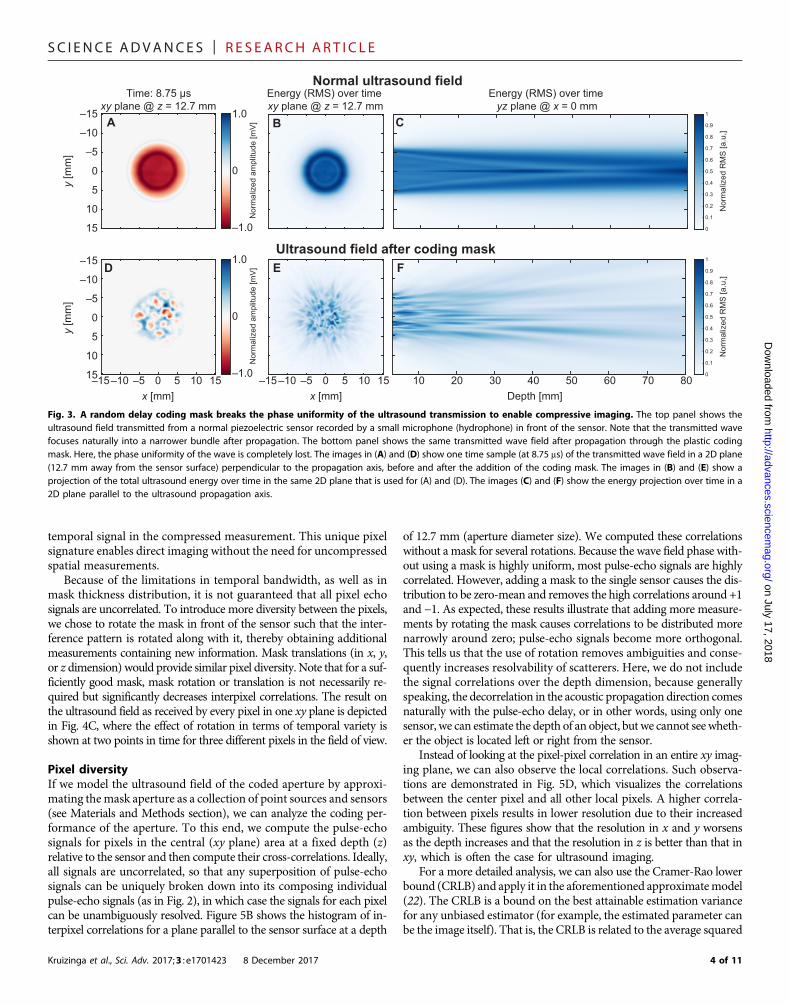
The codingmask placed in front of the ultrasound sensor consistsof a plastic material that supports ultrasound propagation with a speedof around 2750m/s, in contrast to the speed inwater, which is 1480m/sat room temperature. Varying the mask thickness consequently variesthe time the ultrasoundwave spends within the plastic before enteringthe medium, in our case water. For an ultrasound wave with a centralfrequency of 5 MHz to be delayed by a full wavelength with respect tothe rest of the wave requires a local thickness increase of 641 mm.Whenthe thickness of the plastic varies spatially, the phase uniformity of thepropagating wave is broken, initiating a random deterministic interfer-ence pattern in the medium. The mask covers the complete apertureof the sensor (diameter, 12.7mm), and the thickness randomly variesbetween 0.1 and 1mm. Formore details, see theMaterials andMethodssection. It is important to note that the mask generates an interferencepattern that essentially stretches in four dimensions (three spatial andone temporal). So for every location in 3D space (every pixel), we haveone unique ultrasound signal that originates from that location. Figure 3and movie S1 show how the natural focusing of the ultrasound sensoris altered after we place our coding mask in front of the sensor.

Kruizinga et al., Sci. Adv. 2017;3 : e1701423 8 December 2017

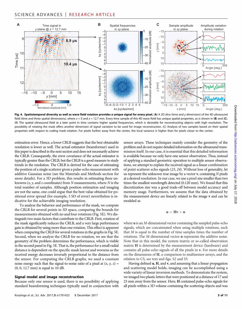
After excitation with a short high-voltage pulse, the piezo sensorused to insonify the medium produces a short ultrasound burst. Al-though short, the limited bandwidth ensures the burst has a certainlength (time) and contains several (positive-negative) cycles. After prop-agating through the mask, the pulse length increases further due to thedistortion of the wavefront by the coding mask (Fig. 4A). These waveswill propagate spherically in themedium andwill interfere constructivelyand destructively, a process that stretches out longer in time than anundistorted wavefront does. Consequently, the available spatial band-width increases compared to anundistorted burst by amask-less sensor.This effect is highlighted in Fig. 4B, which shows two spatial frequencyspectra: one at the beginning of the pulse and one spectrum a fewmicroseconds later. Here, we assume thatmost of the acoustic energyis directly transmitted through the coding mask; yet, in reality, someof the energy will be reflected back from the mask-water interfaceand possibly redirected in the medium through the mask in a secondpass after bouncing back from the mask-transducer interface, therebyincreasing the spatial variability even more.

Any ultrasound imaging problem requires information about thespatial ultrasound field, typically acquired by array sampling. Bymodel-ing the aperture mask as a collection of point sensors, each havingdifferent transmit/receive delays, the mask can still be regarded as asensor array. However, all these point sensor signals are subsequentlysummed by the piezo sensor just after they have passed though themask, resulting in a single compressed measurement, as depicted inthe right panel of Fig. 1 (for a further comparison between a sensorarray and a single sensorwith a codingmask, see text S2 and figs. S1 andS2). The delays produced by the mask create complex spatiotemporalinterference patterns that ensure that each pixel generates a unique

Object 1

+ =

+

+

+

Image 1

Image 3

Image 2

Image 1+ = +

Transmitter / receiver

Transmitter / receiver with coding mask

Object 2

Object 1

Object 2

Computational image reconstruction

Computational image reconstruction

?

?

?

!

A

B

Fig. 2. A spatiotemporally varying ultrasound field allows for compressive imaging. (A) One sensor (transmitter and receiver) cannot distinguish between twoobjects when the transmitted wave field has no spatiotemporal diversity. (B) A simple coding mask can introduce a spatiotemporally varying wave field, which allowsunique signal separation between two objects.

3 of 11

SC I ENCE ADVANCES | R E S EARCH ART I C L E

on July 17, 2018http://advances.sciencem

ag.org/D

ownloaded from

temporal signal in the compressed measurement. This unique pixelsignature enables direct imaging without the need for uncompressedspatial measurements.

Because of the limitations in temporal bandwidth, as well as inmask thickness distribution, it is not guaranteed that all pixel echosignals are uncorrelated. To introduce more diversity between the pixels,we chose to rotate the mask in front of the sensor such that the inter-ference pattern is rotated along with it, thereby obtaining additionalmeasurements containing new information. Mask translations (in x, y,or z dimension) would provide similar pixel diversity. Note that for a suf-ficiently good mask, mask rotation or translation is not necessarily re-quired but significantly decreases interpixel correlations. The result onthe ultrasound field as received by every pixel in one xy plane is depictedin Fig. 4C, where the effect of rotation in terms of temporal variety isshown at two points in time for three different pixels in the field of view.

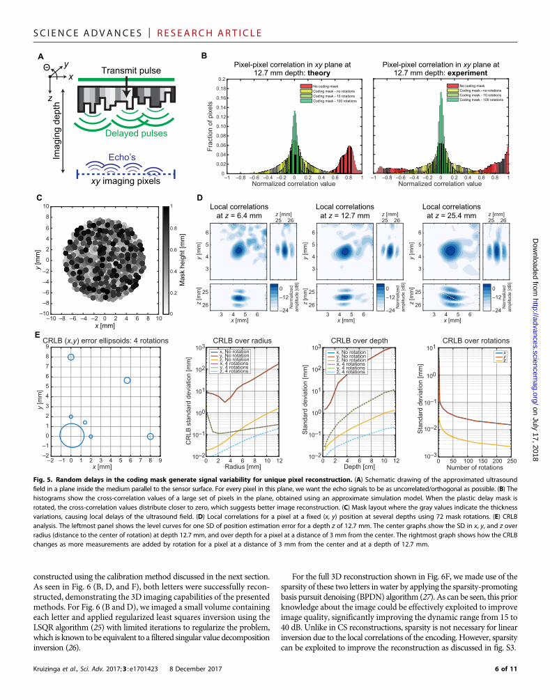
Pixel diversityIf we model the ultrasound field of the coded aperture by approxi-mating themask aperture as a collection of point sources and sensors(see Materials and Methods section), we can analyze the coding per-formance of the aperture. To this end, we compute the pulse-echosignals for pixels in the central (xy plane) area at a fixed depth (z)relative to the sensor and then compute their cross-correlations. Ideally,all signals are uncorrelated, so that any superposition of pulse-echosignals can be uniquely broken down into its composing individualpulse-echo signals (as in Fig. 2), in which case the signals for each pixelcan be unambiguously resolved. Figure 5B shows the histogram of in-terpixel correlations for a plane parallel to the sensor surface at a depth

Kruizinga et al., Sci. Adv. 2017;3 : e1701423 8 December 2017

of 12.7 mm (aperture diameter size). We computed these correlationswithout amask for several rotations. Because the wave field phase with-out using a mask is highly uniform, most pulse-echo signals are highlycorrelated. However, adding a mask to the single sensor causes the dis-tribution to be zero-mean and removes the high correlations around +1and −1. As expected, these results illustrate that adding more measure-ments by rotating the mask causes correlations to be distributed morenarrowly around zero; pulse-echo signals become more orthogonal.This tells us that the use of rotation removes ambiguities and conse-quently increases resolvability of scatterers. Here, we do not includethe signal correlations over the depth dimension, because generallyspeaking, the decorrelation in the acoustic propagation direction comesnaturally with the pulse-echo delay, or in other words, using only onesensor, we can estimate the depth of an object, but we cannot see wheth-er the object is located left or right from the sensor.

Instead of looking at the pixel-pixel correlation in an entire xy imag-ing plane, we can also observe the local correlations. Such observa-tions are demonstrated in Fig. 5D, which visualizes the correlationsbetween the center pixel and all other local pixels. A higher correla-tion between pixels results in lower resolution due to their increasedambiguity. These figures show that the resolution in x and y worsensas the depth increases and that the resolution in z is better than that inxy, which is often the case for ultrasound imaging.

For a more detailed analysis, we can also use the Cramer-Rao lowerbound (CRLB) and apply it in the aforementioned approximatemodel(22). The CRLB is a bound on the best attainable estimation variancefor any unbiased estimator (for example, the estimated parameter canbe the image itself). That is, the CRLB is related to the average squared

0

–15

–10

–5

5

10

15

y [m

m]

Energy (RMS) over time yz plane @ x = 0 mm

10 20 30 40 50 60 70 80Depth [mm]

Time: 8.75 μs xy plane @ z = 12.7 mm

–1.0

0

1.0N

orm

aliz

ed a

mpl

itude

[mV

]

Normal ultrasound field

Ultrasound field after coding mask

–15–10 –5 10 15x [mm]

0 5

0

–15

–10

–5

5

10

15

y [m

m]

–1.0

0

1.0

Nor

mal

ized

am

plitu

de [m

V]

–15–10 –5 10 15x [mm]

0 5

Energy (RMS) over time xy plane @ z = 12.7 mm

A (b)

Nor

mal

ized

RM

S [a

.u,]

0

0.1

0.2

0.3

0.4

0.5

0.6

0.7

0.8

0.9

1

Nor

mal

ized

RM

S [a

.u,]

0

0.1

0.2

0.3

0.4

0.5

0.6

0.7

0.8

0.9

1

B C

ED F

Fig. 3. A random delay coding mask breaks the phase uniformity of the ultrasound transmission to enable compressive imaging. The top panel shows theultrasound field transmitted from a normal piezoelectric sensor recorded by a small microphone (hydrophone) in front of the sensor. Note that the transmitted wavefocuses naturally into a narrower bundle after propagation. The bottom panel shows the same transmitted wave field after propagation through the plastic codingmask. Here, the phase uniformity of the wave is completely lost. The images in (A) and (D) show one time sample (at 8.75 ms) of the transmitted wave field in a 2D plane(12.7 mm away from the sensor surface) perpendicular to the propagation axis, before and after the addition of the coding mask. The images in (B) and (E) show aprojection of the total ultrasound energy over time in the same 2D plane that is used for (A) and (D). The images (C) and (F) show the energy projection over time in a2D plane parallel to the ultrasound propagation axis.

4 of 11

SC I ENCE ADVANCES | R E S EARCH ART I C L E

on July 17, 2018http://advances.sciencem

ag.org/D

ownloaded from

estimation error. Hence, a lower CRLB suggests that the best obtainableresolution is lower as well. The actual estimator (beamformer) used inthis paper is described in the next section anddoes not necessarily achievethe CRLB. Consequently, the error covariance of the actual estimator istypically greater than the CRLB, but the CRLB is a goodmeasure to studytrends in the resolution. The CRLB is derived for the case of estimatingthe position of a single scatterer given a pulse-echomeasurement withadditive Gaussian noise (see the Materials and Methods section formore details). For a 3D problem, this results in estimating three un-knowns (x, y, and z coordinates) fromNmeasurements, whereN is thetotal number of samples. Although position estimation and imagingare not the same, one could argue that the best value obtained for po-sitional error spread (for example, 3 SD of error) nevertheless is in-dicative for the achievable imaging resolution.

To analyze the behavior and performance of the mask, we computethe CRLB for several points in 3D space, comparing the bounds formeasurements obtained with no and four rotations (Fig. 5E).We dis-tinguish twomain factors that contribute to the CRLB. First, rotation ofthe mask significantly reduces the CRLB, and a very large performancegain is obtained by usingmore than one rotation. This effect is apparentwhen comparing theCRLB for several rotations in the graphs in Fig. 5E.Second, when we analyze the CRLB for no rotation, we see that thegeometry of the problem determines the performance, which is visiblein the second panel in Fig. 5E. That is, the performance for a small radialdistance is dependent on the specific mask layout and worsens as thereceived energy decreases inversely proportional to the distance fromthe sensor. For computing the CRLB graphs, we used a constantnoise energy such that the signal-to-noise ratio of a pixel at (x, y, z) =(0, 0, 12.7 mm) is equal to 10 dB.

Signal model and image reconstructionBecause only one sensor is used, there is no possibility of applyingstandard beamforming techniques typically used in conjunction with

Kruizinga et al., Sci. Adv. 2017;3 : e1701423 8 December 2017

sensor arrays. These techniques mainly consider the geometry of theproblemanddonot require detailed informationon the ultrasound trans-mission itself. In our case, it is essential that this detailed informationis available because we only have one sensor observation. Thus, insteadof applying a standard geometric operation to multiple sensor observa-tions, we attempt to explain the received signal as a linear combinationof point scatterer echo signals (23, 24). Without loss of generality, letus represent the unknown true image by a vector v, containingN pixelsat a desired resolution. In our case, we use a pixel size smaller than twotimes the smallest wavelength detected (0.120 mm).We found that thisdiscretization size was a good trade-off between model accuracy andmemory usage. Furthermore, we assume that the data obtained bythe measurement device are linearly related to the image v and can bemodeled as

u ¼ Hv þ n

where u is anM-dimensional vector containing the sampled pulse-echosignals, which are concatenated when using multiple rotations, suchthat M is equal to the number of time samples times the number ofrotations. The M-dimensional vector n represents the additive noise.Note that in this model, the system matrix or so-called observationmatrix H is determined by the measurement device (hardware) andcontains all pulse-echo signals of all the pixels in v. For more detailson the dimensions ofH, a comparison to multisensor arrays, and therelation to CS, see text and figs. S2 and S3.

Having defined u,H, and v, and assuming that a linear propagationand scattering model holds, imaging can be accomplished using awide variety of linear inversionmethods. To demonstrate the system,we imaged two plastic letters thatwere positioned at a distance of 17 and23 mm away from the sensor. Here,H contained pulse-echo signals forall pixels within a 3D volume containing the scattering objects and was

–10 1

–101

0 359Angle [deg.]

–101

Amplitude variation during rotation

0

–15

–10

–5

5

10

15

y [m

m]

Sample amplitude in xy plane

A

–5–4–3–2–1

01234

ky [c

ycle

s/m

m]

5

Spatial frequencies in xy plane

9

10

11

12

Tim

e [u

s]

–15 –10 –5 10 15y [mm]

0 5

8.9 µs

10.4 µs

Time signal in y plane @ z = 12.7 mm

–101

–101

0 359Angle [deg.]

–101

0

–15

–10

–5

5

10

15

y [m

m]

–15–10 –5 10 15x [mm]

0 5

CB

–40

0

Nor

mal

ized

am

plitu

de [d

B]

–10

–20

–30

–4 –2kx [cycles/mm]

–5–4–3–2–101234

ky [c

ycle

s/m

m]

5–3–5 –1 0 21 3 54–1.0 0 1.0

Normalized amplitude [mV]

–40

0

Nor

mal

ized

am

plitu

de [d

B]

–10

–20

–30

Fig. 4. Spatiotemporal diversity as well as wave field rotation provides a unique signal for every pixel. (A) A 2D slice (time and y dimension) of the 4D ultrasoundfield (time and three spatial dimensions), where x = 0 and z = 12.7 mm. Every time sample of this 4D wave field has unique spatial properties, as is shown in (B) and (C).(B) The spatial ultrasound field at a later point in time contains higher spatial frequencies, which is desirable for reconstructing objects with high resolution. Thepossibility of rotating the mask offers another dimension of signal variation to be used for image reconstruction. (C) Analysis of two samples based on their spatialproperties with respect to coding mask rotation. For pixels further away from the center, the local variance is higher than for pixels closer to the center.

5 of 11

SC I ENCE ADVANCES | R E S EARCH ART I C L E

on July 17, 2018http://advances.sciencem

ag.org/D

ownloaded from

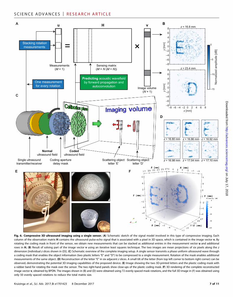
constructed using the calibration method discussed in the next section.As seen in Fig. 6 (B, D, and F), both letters were successfully recon-structed, demonstrating the 3D imaging capabilities of the presentedmethods. For Fig. 6 (B and D), we imaged a small volume containingeach letter and applied regularized least squares inversion using theLSQR algorithm (25) with limited iterations to regularize the problem,which is known to be equivalent to a filtered singular value decompositioninversion (26).

Kruizinga et al., Sci. Adv. 2017;3 : e1701423 8 December 2017

For the full 3D reconstruction shown in Fig. 6F, we made use of thesparsity of these two letters in water by applying the sparsity-promotingbasis pursuit denoising (BPDN) algorithm (27). As can be seen, this priorknowledge about the image could be effectively exploited to improveimage quality, significantly improving the dynamic range from 15 to40 dB. Unlike in CS reconstructions, sparsity is not necessary for linearinversion due to the local correlations of the encoding. However, sparsitycan be exploited to improve the reconstruction as discussed in fig. S3.

Pixel-pixel correlation in xy plane at 12.7 mm depth: theory

Normalized correlation value–1 –0.8 –0.6 –0.4 –0.2 0 0.2 0.4 0.6 0.8 1

0

0.02

0.04

0.06

0.08

0.10

0.12

0.14

0.16

0.18

0.2

Frac

tion

of p

ixel

s

No coding maskCoding mask - no rotationsCoding mask - 10 rotationsCoding mask - 100 rotations

Imag

ing

dept

h

xy imaging pixels

Transmit pulse

z

y

x

Θ

Echo’s

Delayed pulses

0

0.2

0.4

0.6

0.8

1

8

6

4

2

0

–2

–4

–6

–8

10

–10108–8 –6 –4 –2 0 2 4 6–10

x [mm]

y [m

m]

Mas

k he

ight

[mm

]

No coding maskCoding mask - no rotationsCoding mask - 10 rotationsCoding mask - 100 rotations

Normalized correlation value–1 –0.8 –0.6 –0.4 –0.2 0 0.2 0.4 0.6 0.8 1

A B

C D

E

Pixel-pixel correlation in xy plane at 12.7 mm depth: experiment

–2 –1x [mm]

–2

–1

0

1

2

3

4

5

6

7

8

9

y [m

m]

CRLB (x,y) error ellipsoids: 4 rotations

Depth [cm]

Sta

ndar

d de

viat

ion

[mm

]

CRLB over depth

10–2

10–1

100

101

103

102

x, No rotationy, No rotationz, No rotationx, 4 rotationsy, 4 rotationsz, 4 rotations

10 1286420Radius [mm]

CR

LB s

tand

ard

devi

atio

n [m

m]

CRLB over radiusx, No rotationy, No rotationz, No rotationx, 4 rotationsy, 4 rotationsz, 4 rotations

10–2

10–1

100

101

103

102

10 12864200 1 2 3 4 5 6 7 8 9 50 100 150 200 250Number of rotations

10–3

10–2Sta

ndar

d de

viat

ion

[mm

]

CRLB over rotationsx

y

z

10–1

100

101

0

Local correlations at z = 25.4 mm

3

5

6

3 4 6

25

26–24

–120

25 26

Nor

mal

ized

ampl

itude

[dB

]

y [m

m]

z [m

m]

x [mm]

z [mm]

4

5

Local correlations at z = 12.7 mm

3

5

6

3 4 6

25

26–24

–120

25 26

Nor

mal

ized

ampl

itude

[dB

]

y [m

m]

z [m

m]

x [mm]

z [mm]

4

5

Local correlations at z = 6.4 mm

3

5

6

3 4 6

25

26–24

–120

25 26

Nor

mal

ized

ampl

itude

[dB

]

y [m

m]

z [m

m]

x [mm]

z [mm]

4

5

Fig. 5. Random delays in the coding mask generate signal variability for unique pixel reconstruction. (A) Schematic drawing of the approximated ultrasoundfield in a plane inside the medium parallel to the sensor surface. For every pixel in this plane, we want the echo signals to be as uncorrelated/orthogonal as possible. (B) Thehistograms show the cross-correlation values of a large set of pixels in the plane, obtained using an approximate simulation model. When the plastic delay mask isrotated, the cross-correlation values distribute closer to zero, which suggests better image reconstruction. (C) Mask layout where the gray values indicate the thicknessvariations, causing local delays of the ultrasound field. (D) Local correlations for a pixel at a fixed (x, y) position at several depths using 72 mask rotations. (E) CRLBanalysis. The leftmost panel shows the level curves for one SD of position estimation error for a depth z of 12.7 mm. The center graphs show the SD in x, y, and z overradius (distance to the center of rotation) at depth 12.7 mm, and over depth for a pixel at a distance of 3 mm from the center. The rightmost graph shows how the CRLBchanges as more measurements are added by rotation for a pixel at a distance of 3 mm from the center and at a depth of 12.7 mm.

6 of 11

SC I ENCE ADVANCES | R E S EARCH ART I C L E

on July 17, 2018http://advances.sciencem

ag.org/D

ownloaded from

=

Predicting acoustic wavefield by forward propagation and

autoconvolutionOne measurement for every rotation

×

Single ultrasound transmitter/receiver

Normal ultrasound field

Coding aperture delay mask

Coded ultrasound field

Scattering object letter ‘D’

Measurements(M × 1)

Sensing matrix (M × N (M < N))

Scattering object letter ‘E’

Stacking rotationmeasurements

Image volume(N × 1)

x [mm]

86420

–2–4–6–8

y [m

m]

–8 –6 –4 –2 0 2 4 6 8

–15

–10

–5

0

Nor

mal

ized

am

plitu

de [d

B]

86420

–2–4–6–8

y [m

m]

z = 16.80 mm z = 16.86 mm z = 16.92 mm

z = 16.98 mm z = 17.04 mm z = 17.10 mm

H vu

z = 23.4 mm

z = 16.8 mmB

E

C

A

D

F

Fig. 6. Compressive 3D ultrasound imaging using a single sensor. (A) Schematic sketch of the signal model involved in this type of compressive imaging. Eachcolumn of the observation matrix H contains the ultrasound pulse-echo signal that is associated with a pixel in 3D space, which is contained in the image vector v. Byrotating the coding mask in front of the sensor, we obtain new measurements that can be stacked as additional entries in the measurement vector u and additionalrows in H. (B) Result of solving part of the image vector v using an iterative least squares technique. The two images are mean projections of six pixels along the zdimension [individual z slices shown in (D)]. (C) Schematic overview of the complete imaging setup. A single sensor transmits a phase uniform ultrasound wave througha coding mask that enables the object information (two plastic letters “E” and “D”) to be compressed to a single measurement. Rotation of the mask enables additionalmeasurements of the same object. (D) Reconstruction of the letter “E” in six adjacent z slices. A small tilt of the letter (from top left corner to bottom right corner) can beobserved, demonstrating the potential 3D imaging capabilities of the proposed device. (E) Image showing the two 3D-printed letters and the plastic coding mask witha rubber band for rotating the mask over the sensor. The two right-hand panels show close-ups of the plastic coding mask. (F) 3D rendering of the complete reconstructedimage vector v, obtained by BPDN. The images shown in (B) and (D) were obtained using 72 evenly spaced mask rotations, and the full 3D image in (F) was obtained usingonly 50 evenly spaced rotations to reduce the total matrix size.

Kruizinga et al., Sci. Adv. 2017;3 : e1701423 8 December 2017 7 of 11

SC I ENCE ADVANCES | R E S EARCH ART I C L E

on Juhttp://advances.sciencem

ag.org/D

ownloaded from

Constructing the system matrix HFor computing the column signals ofH, it is crucial to know the entirespatiotemporal wave field. To this end, we adopt a simple calibrationmeasurement in which we spatially map the impulse signal (using asmall hydrophone and a translation stage) in a plane close to the masksurface and perpendicular to the ultrasound propagation axis (Fig. 6C).This recorded wave field can then be propagated to any plane that isparallel to the recorded plane using the angular spectrum approach(28, 29). Note that this procedure is required only once and is uniquefor the specific sensor and coding mask. According to the reciprocitytheorem, we are able to obtain the pulse-echo signal by performing anautoconvolution of the propagated hydrophone signal with itself (30).Using these components, we can then compute the pulse-echo ultrasoundsignal for every point in 3D space and subsequently populate the columnsofH.The additional rotation of the codingmask can be regarded as arotation of the ultrasound field inside the medium. Because every rota-tion provides a newmeasurement of the same image v, we canmake useof this information by stacking these new signals as additional rows inthe matrix H. The more independent rows we add to H, the betterconditioned our image reconstruction problem becomes.

More formally, let ui denote the ith sampled pulse-echo signal oflength K, where K is the number of temporal samples obtained fromone pulse-echo measurement and i indexes the various measurementsobtained fromdifferent rotation angles. LetHi denote themeasurementmatrix for rotation i of size K × N, where N is the number of pixels.Then, if R rotations are performed, u andH are defined as follows:u ¼½uT0 uT1 … uTR�1�T andH ¼ ½HT

0 HT1 … HT

R�1�T, where u is lengthM,withM = KR, and H has sizeM × N. Furthermore, because each Hi isobtained by propagating and rotating the same calibration measure-ment (see “Acoustic calibration procedure” section in the Materials andMethods), each Hi can be computed from a reference measurementmatrix ~H:Hi ¼ f ð~H; fiÞ, where fi is the angle of rotation correspondingto measurement i, and the function f(H, fi) computes the matrixHi

from the reference matrix ~H and input angle fi by appropriately rotat-ing the acoustic field implicitly stored in ~H. Consequently,H is expressedas H ¼ ½ f ð~H; f1ÞT fð~H; f2ÞT … fð~H; fR�1ÞT�T.

ly 17, 2018

DISCUSSIONWehave demonstrated that compressive 3D ultrasound imaging can besuccessfully performed using just a single sensor and a simple aperturecoding mask, instead of the thousand or more sensors conventionallyrequired. The plastic mask breaks the phase uniformity of theultrasound field and causes every pixel to be uniquely identifiablewithinthe received signal. The compressed measurement contains thesuperimposed signals from all object pixels. The objects can be resolvedusing a regularized least squares algorithm, as we have proved here bysuccessfully imaging two letters (“E” and “D”). Furthermore, we haveprovided an in-depth analysis of the qualities of our coding aperturemask for compressive ultrasound imaging. We believe that this tech-nique will pave the way for an entirely new means of imaging in whichthe complexity is shifted away from the hardware side and toward thepower of computing.

The calibration procedure that we use and our imaging device bothshare common ideas with the time-reversal work conducted by Finkand co-workers (30–34). Time-reversal ultrasound entails the notionthat any ultrasound field can be focused back to its source by re-emitting the recorded signal back into the same medium. Conse-quently, the ultrasonic waves can be focused onto a particular point

Kruizinga et al., Sci. Adv. 2017;3 : e1701423 8 December 2017

in space and time if the impulse signal of that point is known. Usinga reverberant cavity to create impulse signal diversity and a limitednumber of sensors, Fink et al. have shown that a 3D medium can beimaged by applying transmit focusing with respect to every spatial lo-cation. Hence, they need as many measurements as there are pixels,resulting in an unrealistic scenario for real-time imaging. Our workdiffers in the fact that rather than focusing our ultrasound waves to asingle point, we encode the whole 3D volume onto one spatiotemporalvarying ultrasound field, from which we then reconstruct an imagebased on solving a linear signal model. This has the advantage of re-quiring only a fewmeasurements to image an entire 3D volume, in con-trast to time-reversal work. This difference in acquisition time is crucialformedical imagingwhere the object changes over time, for example, ina beating heart. Another important distinction is the small impedancedifference between our coding mask and imaging medium (less than afactor of 2). As a consequence, there is very little loss of acoustic energyas compared to reverberant cavities that inherently require high im-pedance mismatch to ensure signal diversity (33, 34).

Besides the time-reversal work, our technique also shares somecommon ground with the 2D localization work by Clement et al.(35–37). They successfully showed that frequency-dependent wave fieldpatterns can be used to localize two point scatterers in a 2D planeusing only one sensor in receive. Instead of solving a linear system aswe propose here, the authors used a dictionary containing measuredimpulse responses and a cross-correlation technique to find the twopoint scatterers. By contrast, we propose to induce signal diversity usinglocal delays in both transmit and receive. This type of “wave fieldcoding” can be applied to many other imaging techniques and seemsto offer a much higher dynamic range than the slowly varying frequency-dependent wave fields. As a result, we are able to move beyond the lo-calization of isolated point scatterers but perform actual 3D imaging aswe show in this paper.

The findings reported in this paper demonstrate that compressiveimaging in ultrasound using a coded aperture is possible and practicallyfeasible. Our device has disadvantages and limitations and does notdeliver similar functionality as existing 3Dultrasound arrays. For exam-ple, we cannot focus the transmission beam,making techniques such astissue harmonic imaging that require high acoustic power less accessible(37). In addition, the mechanical rotation of the mask is expected tointroduce a fair amount of error in the prediction of the ultrasound fieldand limits the usability when it comes down to imaging moving tissueor the application of ultrasound Doppler. Besides, a rotating wave fieldbecomes less effective at pixels closer to the center of rotation—assuming a spatially uniform generation of spatial frequencies. Futuresystems should consider the incorporation of other techniques to intro-duce signal variation, such as controlled linearized motion, or a maskthat can be controlled electronically, similar to the digitalmirror devicesused in optical compressive imaging (13). Furthermore, the angularspectrum approach method that predicts the ultrasound field insidethe medium is not flawless in cases where the medium contains strongvariations in sound speed and density. These issues may possibly besolved, however, by incorporating more advanced ultrasound fieldprediction tools that can deal with these kinds of variations (38). Thiswill increase the computational burden of the image reconstructioneven further butmay potentially lead to better results thanwhatwe haveshown here.

One of the fundamental ideas of this paper is to prove that spatialwave compression allows for compressive imaging. Hence, this tech-nique is applicable not only to ultrasound but also tomany other imaging

8 of 11

SC I ENCE ADVANCES | R E S EARCH ART I C L E

Dow

nloaded

and localization techniques that normally rely on spatial sampling of co-herent wave fields.With respect to clinical ultrasound, we believe that theproposed technique may prove to be useful in cases where signal reduc-tion is beneficial, for example, in minimally invasive imaging cathe-ters. Furthermore, we think that a coded aperture mask could potentiallybe used in conjunction with conventional 1D ultrasound arrays to betterestimate the out-of-plane signals and possibly extend the normal 2Dimaging capabilities to 3D.

Alternative coded aperture implementations for ultrasound com-pressive imaging are certainly possible. However, the range of the phys-ical parameters that we can vary to create a useful coded aperture forultrasound seems less diverse compared to optics. The properties oflight are such that it can easily be blocked very locally (for example, byabsorption), which is hardly possible with ultrasound waves because oftheir mechanical nature and larger wavelengths. The idea of applyinglocal delays in the ultrasound field to uniquely address every pixel there-fore seems more practical. Ultimately, it will be these kinds of physicalparameters that will dictate whether and to what extent true compres-sive imaging is possible. Restricting ourselves to local time delays, wehave successfully shown in this paper that the physics of ultrasoundallow for the ultimate compression of a 3D volume in a fewmeasure-ments with a single sensor and a simple coding mask.

on July 17, 2018http://advances.sciencem

ag.org/from

MATERIALS AND METHODSMask manufacturingOur aim was to make a spatiotemporally varying ultrasound field bylocally introducing phase shifts in the wave transmitted by the sensor.We did so by introducing a mask that delays the wave locally, similarto the function of a phase spatial light modulator in optics (39). Theaberration mask that we put in front of the sensor was made from an11-mm-thin circular plastic layer (Perspex), in which we had drilledholes 1 mm in diameter (Fig. 5C). The depth and positions of theseholes were randomly chosen by an algorithm, allowing for a depth ran-ging between 0.1 and 1 mm and for a maximum of 0.5-mm overlapbetween the holes. The holes were drilled using a computer numericcontrol machine (P60 HSC, Fehlmann). The choice for 1-mm holeswasmade because of convenience of manufacturing. At room tempera-ture, the speed of sound propagation in water is approximately 1480m/s,whereas the speed of sound in the Perspexmaterial is 2750m/s. Perspexhas good properties in terms of processing, high sound speed, and lowacoustic absorption.

Acoustic setupFor the transmission and reception of ultrasonic waves, we used onelarge sensor of piezocomposite material that had an active diameterof 12.7 mm and a center frequency of 5 MHz (C309-SU, OlympusPanametrics NDT Inc.). The sensor was coupled to a pulser/receiver box(5077PR, Olympus Panametrics NDT Inc.) that can generate a short−100 V transmit spike and amplifies signals in receive up to 59dB. Nofiltering was applied in receive. The sensor with the mask was mountedin a tank filled with watermeasuring 200 × 300 × 200mm. In the water,we placed two plastic letters that had been 3D-printed (Objet30,Stratasys Ltd.). To enhance the ultrasound reflection from these letters,we sprayed only the letters with silicon carbide powder (size, k800).The two letters “E” and “D” refer to the names of our academic in-stitutions, ErasmusMedical Center andDelft University of Technology.

The thin plastic coding mask was part of a larger round casing thatfitted snugly around the sensor (Fig. 6E). To this casing, we fitted a

Kruizinga et al., Sci. Adv. 2017;3 : e1701423 8 December 2017

cogwheel that allows the casing to be rotated in front of the sensor usinga small rubber band and an electronic rotary stage (T-RS60A, ZaberTechnologies). By rotating the aberrationmask, wewere essentially ableto rotate the interference pattern inside the stationarymedium, allowingfor multiple observations of the same object. We allowed a thin waterfilm between the plastic mask and the sensor surface to ensure optimalcoupling between the piezo material and the plastic mask. With thissetup, it took about 1 min to acquire the signals needed to reconstructthe 3D volume shown in Fig. 6.

Acoustic calibration procedureBefore we could use our device for imaging, we needed to know thesignature of our interference pattern. That is, we needed to know whatthe transmission and receive wave fields looked like in both space andtime, so that we could populate our system matrix H. Note that forevery spatial point, we had a unique temporal ultrasound signal. Thiscalibration step is an essential component in this kind of compressiveimaging (40). The betterH is known, the better the reconstruction ofthe image. For our calibration procedure, we recorded the transmissionwave field in a plane perpendicular to the ultrasound propagation axisusing a 3D translation stage (BiSlide MN10-0100-M02-21, Velmex)and a broadband needle hydrophone (0.5 to 20MHz, 0.2-mmdiameter;Precision Acoustics) coupled to a programmable analog-to-digital con-verter (DP310, Acqiris USA) using 12 bits per sample and a 200-MHzsampling rate.

For the results presented in this paper, we recorded the wave fieldin a 30 × 30mmplane located 2.5mm in front of the aberrationmaskusing a step size of 0.12 mm (less than two times the highest spatialfrequency detected) in both the x and y directions (Figs. 3 and 4). Thesignal of every pixel was obtained using the angular spectrum approachto address pixels at greater depth, using autoconvolution to account forthe pulse-echo acquisition, and using linear interpolation to account foradditional rotation measurements; all of which were implemented inMATLAB software, release 2015b (The MathWorks). We noticed thatour sensor was not completely axisymmetric, meaning that the maskwave interaction changes slightly upon mask rotation. This issue wassolved by measuring four rotated planes (0°, 90°, 180°, and 270°). Wegenerated all intermediate planes by linear interpolation betweeneach pair of neighboring planes. The calibration procedure took around1.5 hours, after which the complete spatiotemporal impulse response ofthe sensor was known. Note that this calibration is sensor- and mask-specific and, in principle, only needs to be done once.

Approximate model and CRLBTo analyze the CRLB for the estimation of a single scatterer from oneormore pulse-echomeasurements, we derived the expressions for com-puting the Fisher information matrix, the inverse of which was com-puted numerically to obtain the CRLB covariance matrix. The followingassumptions and conventions were used:

(i) Any noise or other errors can be modeled as zero mean whiteGaussian additive noise, with variance s2. Hence, this analysis is onlyvalid if noise sources, such as electronic, quantization, or jitter noise,can be modeled as Gaussian random variables, and their total effect iscompounded into the signal-to-noise figure.

(ii) The ultrasound field due to the coding mask can be approxi-mated as a collection of point sources, where the point sources are locatedat the surface of the mask. The point in time at which each virtual pointsource is excited is determinedby the time of arrival of the ultrasound fieldfrom the true sensor location through the mask to the end of the mask.

9 of 11

SC I ENCE ADVANCES | R E S EARCH ART I C L E

on July 17, 2018http://advances.sciencem

ag.org/D

ownloaded from

(iii) The impulse response for the main sensor is taken as beingequal to a Gaussian pulse: hðtÞ ¼ exp½� t2

2l2�, where l determines thepulse width or frequency bandwidth.

(iv) The origin of the spatial axes corresponds to the center of themain sensor surface, with the sensor lying in the xy plane and the z axisperpendicular to the sensor surface.

(v) The sensor is excited by a single Dirac delta pulse.(vi) The position of the virtual source j is denoted as sj∈R3, and the

set of all sj is denoted as S. Vector variables are indicated by bold type-setting.

(vii) The ith element of a vector k is denoted as [k]i.Under the assumptions above, the forward pressure wave field mea-

sured at position q = [x, y, z]T can be written as

pðt; qÞ ¼ ∑Sj j�1

j¼0hðt � tðq; sjÞÞ

where tðq; sjÞ ¼ 1c1½sj�z þ 1

c0jjsj � qjj2 . This can be regarded as the

convolution of the sensor impulse response with the mask impulse re-sponse: p(t, q) = h(t) * m(t, q, S). The echo signal can then be ex-pressed as a(t, q) = h(t) * m(t, q, S) * m(t, q, S) * h(t), or simplya(t, q) = p(t, q) * p(t, q), which is equal to the autoconvolution of theforward pressure wave field at q. Under the white Gaussian noiseassumption, it can be shown that the (i, j)-th entry of the Fisher infor-mation matrix IðqÞ∈R3x3 is equal to

IðqÞi;j ¼1s2

∂aðqÞT∂½q�i

∂aðqÞ∂½q�j

where a(q) is a vector representing the discretized signal a(t, q). Next,we derived the derivative of a(q). We started by computing the deriva-tive of a(t, q)

dd½q�i

aðt; qÞ ¼ dd½q�i

pðt; qÞ*pðt; qÞ ¼ dd½q�i ∫

∞

�∞pðt � T; qÞpðT; qÞdT

¼ ∫∞

�∞

dd½q�i

pðt � T; qÞpðT; qÞdT ¼ 2pðt; qÞ* dd½q�i

pðt; qÞ

Using the definition of p(t, q) and t(q, sj), we find that

dd½q�i

pðt; qÞ ¼ ∑Sj j�1

j¼0

½q�i � ½sj�ijjq� sjjj22

hðt � tðq; sjÞÞ

�"

1c0l2

ðt � tðq; sjÞÞ � 1jjq� sjjj2

#

which can be discretized to obtain da(q)/d[q]i for a singlemeasurement.From I(q), the CRLB is found as I(q)−1.

Image reconstructionHere, we formalized our image reconstruction problem in a set oflinear equations u = Hv + n. This formalization allowed for a mul-titude of solvers to be applied to this problem. We applied two in-version methods to find v from u. The first was the least squares estimate,

Kruizinga et al., Sci. Adv. 2017;3 : e1701423 8 December 2017

which finds the image v that minimizes the squared error between themodel Hv and observation u as follows: v̂ ¼ argminv′j u�Hv′j jj22 .This estimate is known to be the minimum variance unbiased estimatorif the linear model is valid, and the noise n is the white Gaussian. Toimplement this estimator, we used the LSQR algorithm (25), which isespecially appropriate for large-scale sparse systems. By limiting thenumber of iterations, one can regularize the reconstruction problem[see, for example, the study by Hansen (26)]; this also allows for balanc-ing of the resolution, the noise robustness, or the contrast.

For the reconstructed letters shown in Fig. 6 (B and D), we usedabout 15 iterations, which took several seconds to compute. The resultsdid not seem to varymuch between 7 and 40 iterations. Above 50 itera-tions, we observed a serious loss in contrast as the algorithm starts to fitthe solution to the noise and errors present in ourHmatrix. For the com-plete reconstruction of the 3D volume shown in Fig. 6F, we applied aBPDN algorithm (27), exploiting the sparsity of the image becausewe were only interested in two reflecting letters in an otherwise emptymedium (water). For this purpose, we chose to use the iterative two-stepshrinkage/thresholding algorithm, named TwIST, using l1-norm regu-larization (41) for implementation, although other algorithms that arecapable of l1-based optimization are also viable. By this approach, weminimized the BPDN cost-function v̂ ¼ argminv′

12 jju�Hv′jj22 þ

ljjv′jj1, where l is a dimensionless scalar that weights the amountof regularization. The BPDN algorithm regularization parameter lwas chosen by defining a region of interest (ROI) containing the re-constructed letters and an ROI outside the letters and computed thecontrast ratio as 20 log10(Iletter/Ibackground) for a range of l values, whereIletter or Ibackground are the average values of |v| over the pixels in thecorresponding ROI.We then chose the l that offered the highest con-trast ratio. Using this procedure, we observed a contrast of 9 dB forregularized least squares and 29 dB for the l1 regularization. For thisproof-of-principle study, it shows that selecting a suitable l is possiblein a similar way as in real-life clinical ultrasound imaging, where theoperator tunes some critical image reconstruction parameters (such asspeed of sound) by visual feedback on image quality. In further research,it should be investigated if l should be tuned for image content or aglobally optimal l can be established. If the latter is the case, an optimall should be established over large sets of training images, and its gen-erality tested on independent test images. The 3D rendering of theletters shown in Fig. 6F were performed using the open-source visual-ization tool ParaView (www.paraview.org) (42).

SUPPLEMENTARY MATERIALSSupplementary material for this article is available at http://advances.sciencemag.org/cgi/content/full/3/12/e1701423/DC1text S1. On the size of the system matrix H.text S2. Comparison with multisensor array imaging.text S3. On the relation to CS.fig. S1. Imaging performance for a single sensor with coding mask and normal sensor arrayswithout coding mask.fig. S2. Image reconstruction example for a sensor array and a single sensor with coding maskfor a comparable amount of measurements.movie S1. A random delay coding mask breaks the phase uniformity of the ultrasoundtransmission to enable compressive imaging.movie S2. Compressive 3D ultrasound imaging using a single sensor.movie S3. Image reconstruction for a multisensor array and a single sensor with rotating codingmask.Reference (43)

REFERENCES AND NOTES1. K. K. Shung, M. Zippuro, Ultrasonic transducers and arrays. IEEE Eng. Med. Biol. Mag.

15, 20–30 (1996).

10 of 11

SC I ENCE ADVANCES | R E S EARCH ART I C L E

on July 17, 2018http://advances.sciencem

ag.org/D

ownloaded from

2. K. E. Thomenius, Evolution of ultrasound beamformers. in 1996 IEEE UltrasonicsSymposium Proceedings (IEEE, 1996), pp. 1615–1622.

3. A. Fenster, D. B. Downey, H. N. Cardinal, Three-dimensional ultrasound imaging. Phys.Med. Biol. 46, R67 (2001).

4. E. Merz, 25 Years of 3D ultrasound in prenatal diagnosis (1989–2014). Ultraschall. Med.36, 3–8 (2015).

5. E. J. Candès, J. Romberg, T. Tao, Robust uncertainty principles: Exact signalreconstruction from highly incomplete frequency information. IEEE Trans. Inf. Theory52, 489–509 (2006).

6. D. L. Donoho, Compressed sensing. IEEE Trans. Inf. Theory 52, 1289–1306 (2006).7. C. E. Shannon, Communication in the presence of noise. PIRE 37, 10–21 (1949).8. R. G. Baraniuk, Compressive sensing [Lecture Notes]. IEEE Signal Process. Mag.

24, 118–121 (2007).9. N. Wagner, Y. C. Eldar, Z. Friedman, Compressed beamforming in ultrasound imaging.

IEEE Trans. Signal Process. 60, 4643–4657 (2012).10. H. Liebgott, A. Basarab, D. Kouame, O. Bernard, D. Friboulet, Compressive sensing in

medical ultrasound, in 2012 IEEE International Ultrasonics Symposium, (IEEE, 2012), pp. 1–6.11. C. Quinsac, A. Basarab, D. Kouamé, Frequency domain compressive sampling for

ultrasound imaging. Adv. Acoust. Vib. 2012, 231317 (2012).12. M. F. Schiffner, G. Schmitz, Fast pulse-echo ultrasound imaging employing compressive

sensing in Proceedings of the IEEE International Ultrasonics Symposium (IUS) (IEEE, 2011),pp 688–691.

13. M. F. Duarte, M. A. Davenport, D. Takhar, J. N. Laska, T. Sun, K. F. Kelly, R. G. Baraniuk,Single-pixel imaging via compressive sampling. IEEE Signal Process. Mag. 25, 83–91(2008).

14. L. Wang, L. Li, Y. Li, H. C. Zhang, T. J. Cui, Single-shot and single-sensor high/super-resolution microwave imaging based on metasurface. Sci. Rep. 6, 26959 (2016).

15. D. Shrekenhamer, C. M. Watts, W. J. Padilla, Terahertz single pixel imaging with anoptically controlled dynamic spatial light modulator. Opt. Express 21, 12507–12518(2013).

16. N Huynh, E. Zhang, M. Betcke, S. R. Arridge, P. Beard, B. Cox, A real-time ultrasonic fieldmapping system using a Fabry Pérot single pixel camera for 3D photoacoustic imaging, inProceedings of SPIE Volume 9323, (International Society for Optics and Photonics, 2015),pp. 93231O.

17. E. Caroli, J. B. Stephen, G. Di Cocco, L. Natalucci, A. Spizzichino Coded aperture imaging inX-and gamma-ray astronomy. Space Sci. Rev. 45, 349–403 (1987).

18. R. F. Marcia, Z. T. Harmany, R. M. Willett, Compressive coded aperture imaging, inProceedings of SPIE Volume 7246, (International Society for Optics and Photonics, 2009),pp. 72460G.

19. X. Peng, G. J. Ruane, G. A. Swartzlander Jr., Randomized aperture imaging. https://arxiv.org/abs/1601.00033 (2016).

20. K. Melde, A. G. Mark, T. Qiu, P. Fischer, Holograms for acoustics. Nature 537, 518–522 (2016).21. M. D. Brown, D. I. Nikitichev, B. E. Treeby, B. T. Cox, Generating arbitrary ultrasound fields

with tailored optoacoustic surface profiles. Appl. Phys. Lett. 110, 094102 (2017).22. S. M. Kay, Fundamentals of statistical signal processing: Estimation Theory, (PTR Prentice-

Hall, 1993).23. R. Lavarello, F. Kamalabadi, W. D. O’Brien, A regularized inverse approach to ultrasonic

pulse-echo imaging. IEEE Trans. Med. Imaging 25, 712–722 (2006).24. R. Stoughton, S. Strait, Source imaging with minimummean-squared error. J. Acoust. Soc. Am.

94, 827–834 (1993).25. C. C. Paige, M. A. Saunders, LSQR: An algorithm for sparse linear equations and sparse

least squares. ACM Trans. Math. Softw. 8, 43–71 (1982).26. P. C. Hansen, Discrete Inverse Problems: Insight and Algorithms (SIAM, 2010).27. S. S. Chen, D. L. Donoho, M. A. Saunders, Atomic decomposition by basis pursuit. SIAM

Rev. Soc. Ind. Appl. Math. 43, 129–159 (2001).28. Y. Du, H. Jensen, J. A. Jensen, Investigation of an angular spectrum approach for pulsed

ultrasound fields. Ultrasonics 53, 1185–1191 (2013).29. P. R. Stepanishen, K. C. Benjamin, Forward and backward projection of acoustic fields

using FFT methods. J. Acoust. Soc. Am. 71, 803–812 (1982).

Kruizinga et al., Sci. Adv. 2017;3 : e1701423 8 December 2017

30. M. Fink, Time reversal of ultrasonic fields. I. Basic principles. IEEE Trans. Ultrason.Ferroelectr. Freq. Control 39, 555–566 (1992).

31. G. Montaldo, D. Palacio, M. Tanter, M. Fink, Building three-dimensional images using atime-reversal chaotic cavity. IEEE Trans. Ultrason. Ferroelectr. Freq. Control 52, 1489–1497(2005).

32. C. Draeger, J.-C. Aime, M. Fink, One-channel time-reversal in chaotic cavities:Experimental results. J. Acoust. Soc. Am. 105, 618–625 (1999).

33. N. Etaix, M. Fink, R. K. Ing, Acoustic imaging device with one transducer. J. Acoust. Soc. Am.131, EL395–EL399 (2012).

34. G. Montaldo, D. Palacio, M. Tanter, M. Fink, Time reversal kaleidoscope: A smarttransducer for three-dimensional ultrasonic imaging. Appl. Phys. Lett. 84, 3879–3881(2004).

35. P. J. White, G. T. Clement, Two-dimensional localization with a single diffuse ultrasoundfield excitation. IEEE Trans. Ultrason. Ferroelectr. Freq. Control 54, 2309–2317 (2007).

36. F. C. Meral, M. A. Jafferji, P. J. White, G. T. Clement, Two-dimensional image reconstructionwith spectrally-randomized ultrasound signals. IEEE Trans. Ultrason. Ferroelectr. Freq.Control 60, 2501–2510 (2013).

37. G. T. Clement, Two-dimensional ultrasound detection with unfocused frequency-randomized signals. J. Acoust. Soc. Am. 121, 636–647 (2007).

38. B. E. Treeby, B. T. Cox, k-Wave: MATLAB toolbox for the simulation and reconstruction ofphotoacoustic wave fields. J. Biomed. Opt. 15, 021314 (2010).

39. N. Savage, Digital spatial light modulators. Nat. Photonics 3, 170–172 (2009).40. A. Liutkus, D. Martina, S. Popoff, G. Chardon, O. Katz, G. Lerosey, S. Gigan, L. Daudet,

I. Carron, Imaging with nature: Compressive imaging using a multiply scattering medium.Sci. Rep. 4, 5552 (2014).

41. J. M. Bioucas-Dias, M. A. T. Figueiredo, A new TwIST: two-step iterative shrinkage/thresholding algorithms for image restoration. IEEE Trans. Image Process. 16, 2992–3004(2007).

42. J. Ahrens, B. Geveci, C. Law, C. Hansen, C. Johnson, 36-ParaView: An End-User Tool forLarge-Data Visualization, in The Visualization Handbook, (Elsevier, 2005), pp. 717–731.

43. E. J. Candes, T. Tao, Decoding by linear programming. IEEE Trans. Inf. Theory51, 4203–4215 (2005).

AcknowledgmentsFunding: This work is part of the PUMA project (project 13154 within the STW Open TechnologyProgramme) and the ASPIRE project (project 14926 within the STW Open TechnologyProgramme), which is financed by the Netherlands Organisation for Scientific Research (NWO).Author contributions: P.K. proposed the concept, performed the experiments, developed thereconstruction code, supervised the project, and contributed to the writing of the paper. P.v.d.Mperformed the experiments, developed the simulation code, analyzed the CRLB, andcontributed to the writing of the paper. A.F. performed the experiments and developed thecode for analysis and reconstruction. F.M. contributed to the discussions on the conceptand the experimental setup and made the reconstruction movies. G.S. manufactured thecoding mask and experimental setup. N.d.J. contributed to the discussions on the concept.J.G.B. and G.L. contributed to the discussions on the concept and writing of the paper.Competing interests: The authors declare that they have no competing interests. Dataand materials availability: All data needed to evaluate the conclusions in the paper arepresent in the paper and/or the Supplementary Materials. Additional data related to this papermay be requested from the authors.

Submitted 2 May 2017Accepted 8 November 2017Published 8 December 201710.1126/sciadv.1701423

Citation: P. Kruizinga, P. van der Meulen, A. Fedjajevs, F. Mastik, G. Springeling, N. de Jong,J. G. Bosch, G. Leus, Compressive 3D ultrasound imaging using a single sensor. Sci. Adv. 3,e1701423 (2017).

11 of 11

Compressive 3D ultrasound imaging using a single sensor

and Geert LeusPieter Kruizinga, Pim van der Meulen, Andrejs Fedjajevs, Frits Mastik, Geert Springeling, Nico de Jong, Johannes G. Bosch

DOI: 10.1126/sciadv.1701423 (12), e1701423.3Sci Adv 

ARTICLE TOOLS http://advances.sciencemag.org/content/3/12/e1701423

MATERIALSSUPPLEMENTARY http://advances.sciencemag.org/content/suppl/2017/12/04/3.12.e1701423.DC1

REFERENCES

http://advances.sciencemag.org/content/3/12/e1701423#BIBLThis article cites 34 articles, 0 of which you can access for free

PERMISSIONS http://www.sciencemag.org/help/reprints-and-permissions

Terms of ServiceUse of this article is subject to the

registered trademark of AAAS.is aScience Advances Association for the Advancement of Science. No claim to original U.S. Government Works. The title

York Avenue NW, Washington, DC 20005. 2017 © The Authors, some rights reserved; exclusive licensee American (ISSN 2375-2548) is published by the American Association for the Advancement of Science, 1200 NewScience Advances

on July 17, 2018http://advances.sciencem

ag.org/D

ownloaded from