Applied Physics - hu-berlin.depeople.physik.hu-berlin.de/~bfmaier/data/fpraktikum/F5l...Humboldt...

FACULTY FOR MATHEMATICS AND NATURAL SCIENCE IDEPARTMENT OF PHYSICS

Applied Physics:Advanced Laboratory

5th experiment:Z0-Resonance

date of experiment 14.06.2011hand in 03.08.2011advisor Gerrit Spengler

experimentalists Lucas HacklBenjamin Maier

Humboldt University of BerlinFaculty for Mathematics and Natural Science I – Department of PhysicsApplied Physics: Advanced Laboratory | Lucas Hackl & Benjamin Maier

Contents

1 Introduction 31.1 Theory . . . . . . . . . . . . . . . . . . . . . . . . . . . . . . . . . . . . . . . . . . . . . . . 3

1.1.1 Standard Model . . . . . . . . . . . . . . . . . . . . . . . . . . . . . . . . . . . . . . 31.1.2 Z0 Resonance . . . . . . . . . . . . . . . . . . . . . . . . . . . . . . . . . . . . . . . 31.1.3 Relevant Quantities . . . . . . . . . . . . . . . . . . . . . . . . . . . . . . . . . . . . 3

1.2 Experimental setup . . . . . . . . . . . . . . . . . . . . . . . . . . . . . . . . . . . . . . . . 31.2.1 L3 Detector . . . . . . . . . . . . . . . . . . . . . . . . . . . . . . . . . . . . . . . . 31.2.2 Luminosity Monitor . . . . . . . . . . . . . . . . . . . . . . . . . . . . . . . . . . . 41.2.3 Track Detector . . . . . . . . . . . . . . . . . . . . . . . . . . . . . . . . . . . . . . 41.2.4 Electromagnetic Calorimeter . . . . . . . . . . . . . . . . . . . . . . . . . . . . . . . 41.2.5 Scintillation Counters . . . . . . . . . . . . . . . . . . . . . . . . . . . . . . . . . . 41.2.6 Hadronic Calorimeter . . . . . . . . . . . . . . . . . . . . . . . . . . . . . . . . . . . 41.2.7 Muonic Calorimeter . . . . . . . . . . . . . . . . . . . . . . . . . . . . . . . . . . . 41.2.8 Surrounding Magnets . . . . . . . . . . . . . . . . . . . . . . . . . . . . . . . . . . . 4

2 Data analysis 42.1 Filter criteria . . . . . . . . . . . . . . . . . . . . . . . . . . . . . . . . . . . . . . . . . . . 4

2.1.1 Selection of hadronic events . . . . . . . . . . . . . . . . . . . . . . . . . . . . . . . 52.1.2 Selection of myonic events . . . . . . . . . . . . . . . . . . . . . . . . . . . . . . . . 5

2.2 Calculation of Breit-Wigner Parameters . . . . . . . . . . . . . . . . . . . . . . . . . . . . . 62.3 Derived parameters . . . . . . . . . . . . . . . . . . . . . . . . . . . . . . . . . . . . . . . . 6

2.3.1 Properties of the Z0 Boson . . . . . . . . . . . . . . . . . . . . . . . . . . . . . . . . 72.3.2 Leptonic Decay Width . . . . . . . . . . . . . . . . . . . . . . . . . . . . . . . . . . 72.3.3 Weinberg Angle . . . . . . . . . . . . . . . . . . . . . . . . . . . . . . . . . . . . . 72.3.4 Number of Quark Colors . . . . . . . . . . . . . . . . . . . . . . . . . . . . . . . . . 8

3 Conclusion 8

Abstract

We searched for Z0 bosons produced in electron-positron-collisions of the L3 detector at LEP (CERN) atcenter-of-mass energies of about

√s≈ 91GeV. We introduced proper selection criteria to distinguish between

Z0 → qq, Z0 → µµ and underground events, comparing with Monte-Carlo simulations. Using these cuts wewere able to determine the mass of the Z0 boson and – by combining the different values of decay rates – tocompute further parameters of the standard model, such as the Z0 decay width, its life-time, the Weinberg angleand the number of colors in the strong interaction.

5th experiment: Z0-Resonance 2


1 Introduction

1.1 Theory

1.1.1 Standard Model

The standard model of particle physics is a quan-tum field theory which includes three of the four fun-damental forces, concretely the electromagnetic, theweak and the strong interaction, whereas gravity isnot considered. The interactions themselves are de-scribed by gauge fields (abelian for the electromag-netic interaction and non-abelian for the other) whoseexcited states are interpreted as vector bosons. In thispicture the subatomic particles we know are describedas quantum fields as well. Roughly speaking, the el-ements in the taylor expansion in the coupling con-stant of the time evolution operator (using quantummechanics for fields with its canonical quantization)can be seen as diagrams and the appearing terms asvertices and edges (propagators). This very convenientway of facing the calculation was introduced and de-veloped by R. Feynman in 1949.A. Salam, S. Glashow and S. Weinberg were able tounify the electromagnetic and the weak interactionwithin one theory, the theory of the electroweak in-teraction. From this point of view the gauge bosons ofthe electroweak interactions are produced by a spon-taneous symmetry breaking of the underlying SU(2)×U(1)γ symmetry to SU(2)×U(1)em. Then, the B0 andW 0 bosons mix up to the real gauge bosons Z0 and γ,whereas the W± bosons still remain unchanged.This gauge group predicts one electrically-neutral,massive gauge boson commonly referred as Z0. Themass mZ and the percentage of B0/W 0 mixing (de-scribed by the Weinberg angle θW ) remain as free pa-rameters of the field theory which have to be deter-mined by experimental setups. Furthermore, the rela-tionship of the two couple constants – the electromag-netic one and that of the weak interaction – is deter-mined by the Weinberg angle as well. Exactly thesesetups were provided by the LEP at CERN (Geneva,Switzerland). We will use the data of about 10000scattering events to determine these two parameters ofthe model. Furthermore, we are able to calculate thedecay width of the process which is connected with itslifetime.

1.1.2 Z0 Resonance

In this experiment we are looking at the process

e+e−→ Z0→ f f̄ ,

where f stands for the possible resulting fermions: theleptons e, µ, τ, their neutrinos νe, νµ, ντ and the quarksu, d, c, s, b (note that the center-of-mass energies ofthe experiment are too small to produce t-pairs). Us-ing Feynman diagrams we can derive the form of theamplitude which contains a factor (because of the mas-sive Z0 propagator)

A≈ 1s−M2

Z + iMZ ΛZ

(with the Mandelstam variable s = p2e− + p2

e+). There-fore, it has a pole at s = M2

Z which we have regulizedby introducing the complex term in the numerator. Foran s close to MZ the propability of producing a Z0 bo-son increases dramatically. At this energy QED effectsare almost eliminated and the processes including Z0

decay becomes maximal. Because of the propagatorthe cross section function σ(

√s) has the form of a

Breit-Wigner curve

σ f = σ0sΓ2

Z(s−M2

Z

)2+M2

Z Γ2Z

(1)

1.1.3 Relevant Quantities

The amplitude σ0 can be calculated considering thedecay widths of the initial state (electron e) and thefinal state (fermion f )

σ0 =12π

M2Z Γ2

ZΓe Γ f , (2)

where the fermionic decay width can be evaluated fol-lowing

Γ f =GF M3

Z

24π√

2

[1+(1−4 |Q f | sin2

θW)2]. (3)

Here, GF = 1.166× 10−5 GeV−2 is Fermi’s constant,θW is the Weinberg mixing angle and Q f is thefermion’s charge (±1 for leptons l±, 0 for their neu-trinos, 2/3 for up-kind quarks and -1/3 for down-kindquarks.

1.2 Experimental setup

1.2.1 L3 Detector

As a collaboration of more than 50 international insti-tutes the L3 experiment built the largest known LEPdetector. It detects particles from electron-positron-annihilation which happens in the LEP tunnel. Thename L3 was chosen due to the fact that it was builtup according to the third draft which was handed in. Itis optimized for measuring the energy as precisely aspossible (for leptons, photons and hadron jets).The detector consists of a number of smaller detectors.



1.2.2 Luminosity Monitor

This element consists of two electromagneticcalorimeters and two sets of wire chambers whichare placed symmetrically on both sides of the interac-tion point. It provides the opportunity to measure theluminosity by Bhabha scattering with a relative preci-sion of 0.3%. However, the luminosity given for ourdata was associated with a relative error of 1%.

1.2.3 Track Detector

The track detector enables us to measure the trajectoryof a particle. It is made up of cylindric scintillator lay-ers to measure the z-direction (which we put parallelto the incoming beams) and of a drift chamber whichensures a low drift velocity by a low diffusion gas mix-ture at proper pressure.

1.2.4 Electromagnetic Calorimeter

Since electrons and positrons mainly interact over theelectromagnetic force (cascades of annihilation andpair production), this calorimeter must take care of aneffective absorbing. In the L3 detector, this is donewith semiconductor detectors of the type Bi4Ge3O12[5], which effectively analyze these electromagneticshowers.

1.2.5 Scintillation Counters

The scintillation counters consist of 30 plastic coun-ters situated between the electromagnetic and hadroniccalorimeters. It is an important element for distin-guishing between Z0 muons and cosmic muons, be-cause the time difference between two events in dif-ferent scintillators are unequal: While a cosmic muonneed about 6ns (because it passes the whole detector),the Z0 muon pair, we are interested in, will activatetwo detectors at the same time.

1.2.6 Hadronic Calorimeter

The hadronic calorimeter has to detect particles whichmainly interact over the strong interaction and for thisreason can pass the scintillation counter. Their energycan be measured considering total absorption: conclu-sively, the main materials in the hadronic calorimetersare those with a high mass number A, since these in-teract strong, as well. In the L3 detector the hadronicchamber is made of several uranium absorber plates.A huge amount of wires ensures that we are able tolocate the place of the energy absorption. It acts as

a calorimeter and filter at the same time because onlynon-showering particles will pass.Since the main particles detected in the hadroniccalorimeters are pions, a detection will be associatedwith the pion mass in the data.

1.2.7 Muonic Calorimeter

The last calorimeter is the muonic calorimeter: Muonsare about 200 times heavier and for this reason they arelikely to pass the electromagnetic calorimeter (energyabsorption is inverse proportional to the mass) and thehadronic one (leptons do not strongly interact). Be-tween hadronic and muonic calorimeter a muon filteris placed which ensures that mainly muons can passinto the last chamber.

1.2.8 Surrounding Magnets

The whole detector is surrounded by a magnetic struc-ture made of iron with a small carbon content. Thecentral field in the magnet is about 0.5T. By re-constructing the circle trajectory of a particle, one isable to determine its charge (considering the Lorentzforce).

2 Data analysis

2.1 Filter criteria

Since the data measured at√

s contains all kind ofevents, it is necessary to find criteria to distinguish be-tween hadronic, muonic and other events. Let P be aset which contains all particles of an event. We mod-ified the event class in our C++ program to calculatecertain information for each event set P, concretely:

• Number of particles in the event

|P|

• Total transversal momentum

ptT =

√∑i∈P

[(px

i )2 +(py

i )2]

• Total momentum

pt =√

∑i∈P

[(px

i )2 +(py

i )2 +(pz

i )2]

• Total energy

Et = ∑i∈P

√(pt

i)2 +m2

i



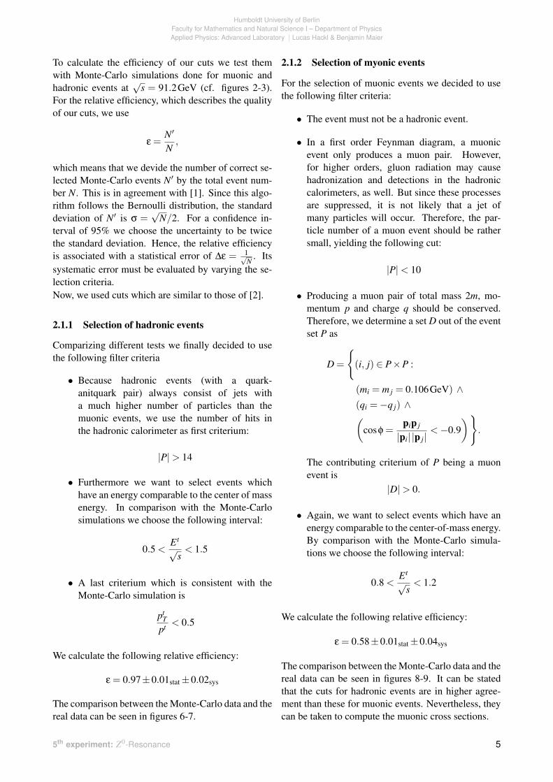
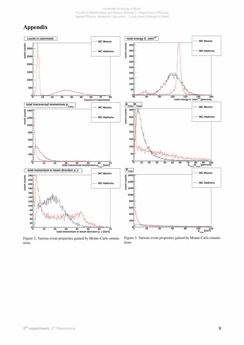
To calculate the efficiency of our cuts we test themwith Monte-Carlo simulations done for muonic andhadronic events at

√s = 91.2GeV (cf. figures 2-3).

For the relative efficiency, which describes the qualityof our cuts, we use

ε =N′

N,

which means that we devide the number of correct se-lected Monte-Carlo events N′ by the total event num-ber N. This is in agreement with [1]. Since this algo-rithm follows the Bernoulli distribution, the standarddeviation of N′ is σ =

√N/2. For a confidence in-

terval of 95% we choose the uncertainty to be twicethe standard deviation. Hence, the relative efficiencyis associated with a statistical error of ∆ε = 1√

N. Its

systematic error must be evaluated by varying the se-lection criteria.Now, we used cuts which are similar to those of [2].

2.1.1 Selection of hadronic events

Comparizing different tests we finally decided to usethe following filter criteria

• Because hadronic events (with a quark-anitquark pair) always consist of jets witha much higher number of particles than themuonic events, we use the number of hits inthe hadronic calorimeter as first criterium:

|P|> 14

• Furthermore we want to select events whichhave an energy comparable to the center of massenergy. In comparison with the Monte-Carlosimulations we choose the following interval:

0.5 <Et√

s< 1.5

• A last criterium which is consistent with theMonte-Carlo simulation is

ptT

pt < 0.5

We calculate the following relative efficiency:

ε = 0.97±0.01stat±0.02sys

The comparison between the Monte-Carlo data and thereal data can be seen in figures 6-7.

2.1.2 Selection of myonic events

For the selection of muonic events we decided to usethe following filter criteria:

• The event must not be a hadronic event.

• In a first order Feynman diagram, a muonicevent only produces a muon pair. However,for higher orders, gluon radiation may causehadronization and detections in the hadroniccalorimeters, as well. But since these processesare suppressed, it is not likely that a jet ofmany particles will occur. Therefore, the par-ticle number of a muon event should be rathersmall, yielding the following cut:

|P|< 10

• Producing a muon pair of total mass 2m, mo-mentum p and charge q should be conserved.Therefore, we determine a set D out of the eventset P as

D =

{(i, j) ∈ P×P :

(mi = m j = 0.106GeV) ∧(qi =−q j) ∧(

cosφ =pip j

|pi| |p j|<−0.9

)}.

The contributing criterium of P being a muonevent is

|D|> 0.

• Again, we want to select events which have anenergy comparable to the center-of-mass energy.By comparison with the Monte-Carlo simula-tions we choose the following interval:

0.8 <Et√

s< 1.2

We calculate the following relative efficiency:

ε = 0.58±0.01stat±0.04sys

The comparison between the Monte-Carlo data and thereal data can be seen in figures 8-9. It can be statedthat the cuts for hadronic events are in higher agree-ment than these for muonic events. Nevertheless, theycan be taken to compute the muonic cross sections.



C.M. Energy Luminosity Hadronic Event Hadronic Cross Muonic Event Muonic Cross√s/GeV L/nb−1 Counts NHad Sections σHad /nb Counts Nµ Sections σµ /nb

89.48±0.89 179.3±1.8 1745 10.04±0.25 72 0.691±0.05091.33±0.91 135.9±1.4 3896 29.57±0.74 140 1.773±0.12793.02±0.93 151.1±1.5 2085 14.23±0.36 85 0.968±0.069

Table 1: Extracted event counts and calculated cross sections

2.2 Calculation of Breit-Wigner Parameters

The curve of the cross section σ(√

s) has the form ofa Breit-Wigner distribution where the resonance takesplace at MZ . Precisely speaking we have to introducea further correction caused by effects of quantum elec-trodynamics, which is done by a program written for[1].To calculate the cross section we use

σ =NL,

with L being the integrated luminosity. As mentioned,it is associated to a relative uncertainty of 1% (as ex-plained in [1]). The measurement of the luminosity isdone by Bhabha scattering at small scattering angleswith specific detector components. This is a pure QEDprocess and for this reason independent from the Z0

properties we will compute. We use the values givenin [1], combined in table 1.To determine the number of events N we analyze thedata with the cuts above, gaining N′. We do not finda significant background. For this reason we try to es-timate the background in a similar way as explainedin [2] on p. 38 (hadronic events) and 41 (muonicevents): We subtract the number of background events(p = 0.15% of N′ for hadronic events and p = 0.7%of N′ for muonic events) and divide by our relative ef-ficiency, yielding

N =(1− p)N′

ε,

respectively

σ =(1− p)N′

εL.

The Gaussian error propagation was used to evaluatethe cross section’s uncertainty. Using these formulas,we gain the results shown in table 1.Now we are able to perform two fits to gain the events’cross section curves. Since the algorithm of minimiz-ing χ2 is performed with zero degrees of freedom, it israther a calculation with error propagation of the Breit-Wigner parameters than a proper fit. The results of thiscalculation may be seen in table 2 and figure 1.

[GeV]1/2

centerofmass energy s80 82 84 86 88 90 92 94 96 98 100

[n

b]

σcro

ss s

ecti

on

0

5

10

15

20

25

30

35

40

Had0

σ 2.147± 39.86

HadZΓ 0.9495± 2.556

HadZM 0.6489± 91.17

Had0

σ 2.147± 39.86

HadZΓ 0.9495± 2.556

HadZM 0.6489± 91.17

BreitWigner curve

QED correction

cross section of hadron events

[GeV]1/2

centerofmass energy s80 82 84 86 88 90 92 94 96 98 100

[n

b]

σcro

ss s

ecti

on

0

0.2

0.4

0.6

0.8

1

1.2

1.4

1.6

1.8

2

2.2

2.4

µ

0σ 0.2158± 2.356

µ

ZΓ 1.102± 2.91

µ

ZM 0.649± 91.19

µ

0σ 0.2158± 2.356

µ

ZΓ 1.102± 2.91

µ

ZM 0.649± 91.19 BreitWigner curve

QED correction

cross section of muon events

Figure 1: Breit-Wigner curves determined from the calculatedcross sections. The results are shown in table 2.

Parameter Hadronic MuonicResult (Had) Result (µ)

σ0 /nb 39.9±2.4 2.46±0.42ΓZ /GeV 2.56±0.95 3.13±1.31MZ /GeV 91.2±0.7 91.1±0.7

Table 2: Parameters gained from Breit-Wigner calculation

2.3 Derived parameters

In this part we will calculate the free parameters ofthe standard model which are determined by the Breit-Wigner parameters. When not stated in another way,we used the Gaussian method of error propagation byaccounting all parameters.



2.3.1 Properties of the Z0 Boson

Since both the results (gained from muonic andhadronic cross sections) are of equal value, we are ableto calculate weighted means1, yielding

MZ = (91.2±0.5)GeV

ΓZ = (2.7±0.7)GeV

τZ = (2.4±0.6)×10−25 s

The Z0 life-time was calculated using the formulaτ = ~/Γ.

2.3.2 Leptonic Decay Width

From Muonic Cross Sections Since both, the initialand the final state of the reaction, are leptonic stateswith |Q f |= 1, we are able to evaluate the leptonic de-cay width using equation (2) to

Γµe = Mµ

Z ΓµZ

√σ

µ0

12π,

yielding the result

Γµe = (106±41)MeV.

The superscript µ denotes that the quantity was gainedusing the results from the muonic cross sections.

From Hadronic Cross Sections Again, using equa-tion (2), we are able to compute the amplitude σ0 ofthe hadronic cross section

σHad0 =

12πΓe ΓH(MHad

Z ΓHadZ

)2 .

The superscript Had denotes that the quantity wasgained using the results from the hadronic cross sec-tions. Since ΓH, the hadronic decay width is notknown, we can use the fact that the Z0 decay widthis the sum of all decay widths

ΓHadZ = ΓH +3Γ

Hadν +3Γ

Hade .

Due to the neutral charge of neutrinos, we are able tocalculate the neutrino decay width using equation (3)

ΓHadν =

GF (MHadZ )3

12π√

2.

Combining all the equations above, we arrive at theleptonic decay width

ΓHade =− 1

2

(GF(MHad

Z)3

12π√

2− ΓHad

Z3

)

±

√14

(GF (MHad

Z )3

12π√

2− ΓHad

Z3

)2

−σHad

0

(MHad

Z

)2 (ΓHad

Z

)2

36π

We are gaining two results using this equation. Hence,we have to compare them with the value from liter-ature Γe = (83.6± 0.8)MeV to determine the physi-cally most likely result

ΓHade = (81±21)MeV.

Final Result Again, both, the muonic and thehadronic results, are of equal value. Hence, we haveno reason to neglect one of them and calculate theweighted mean:

Γe = (87±19)MeV.

2.3.3 Weinberg Angle

The electroweak mixing angle, respectively its squaredsine S2

θ= sin2

θW, can be determined using two differ-ent equations. The first two results may be evaluatedusing equation (3)

S2θ,± =

14

1±

√Γe 24π

√2

GF M3Z−1

. (4)

Referring to [6], the third result can be calculated us-ing the equation

S2θ,3 = 1−M2

W

M2Z,

where MW = (80.399± 0.023)GeV is the W± bosonmass, taken from [7]. For calculating the uncertaintyof the first formula we used a maximum error esti-mation2, since the used quantities are related to eachother. The uncertainty of the second formula is cal-culated with the Gaussian method, as usual. Finally,using the weighted means of the needed parameters,we gain the results

S2θ,+ = 0.303±0.143,

S2θ,− = 0.197±0.143,

S2θ,3 = 0.223±0.008.

1We are using the formulas x̄ = ∑i wixi/∑i wi and ∆x = 1/√

∑i wi with weights wi = 1/∆x2i

2i.e. the formula ∆ f (x) = ∑i∈x ∆xi

∣∣∣ ∂ f∂xi

∣∣∣5th experiment: Z0-Resonance 7


Equations Equation (3) with WeinbergQuantity (3) and (5) + − 3Γν /GeV 0.1658±0.0025ΓH /GeV 1.97±0.78Γd /GeV 0.11±0.02 0.128±0.025 0.124±0.003Γu /GeV 0.086±0.013 0.101±0.032 0.097±0.003

Table 3: Calculated decay widths

Compared to the value given in the literature S2θ=

0.23120± 0.00015 [8], the results S2θ,−, S2

θ,3 seem tobe more likely. However, all the values are right withinin their uncertainty range. Thus, we have to computeall following results with all the values.

2.3.4 Number of Quark Colors

This quantity NC is a factor in the decay width ofquarks ΓH, i.e.

ΓH = NC KQCD (2Γu +3Γd) ,

where KQCD ≈ 1.04 is a factor from Feynman dia-grams of higher orders for gluon radiation [1]. Again,the decay width of hadron events can be examinedfrom the total decay width using

ΓH = ΓZ−3Γν−3Γe, (5)

summing up

NC =ΓZ−3Γν−3Γe

KQCD (2Γu +3Γd) .

The quantities Γu, Γd and Γν can be computed with theelectroweak mixing angle using equation (3). Sincemany of the quantities are related we are using a max-imum error estimation again, yielding the decay widthresults shown in table 3. Finally we gain the values

NC,+ = 3.7±2.1,

NC,− = 3.2±2.0,

NC,3 = 3.4±1.4.

Although all values are in agreement with the expectedvalue NC = 3, they are too high and their uncertaintiesare rather large, too.

3 Conclusion

We were successfully able to extract the number ofevents using the cuts described in section 2.1, to gainthe cross sections, the Breit-Wigner parameters, theleptonic decay width, the electroweak mixing angleand the number of quark colors, summing up the phys-ically most likely results in table 4. They are in agree-ment with the literature.

quantity measured literatureZ0 mass: MZ/GeV 91.2±0.5 91.1876±0.0021

Z0 decay width: ΓZ/GeV 2.7±0.7 2.4952±0.0023Z0 life time: τZ/10−25 s 2.4±0.6 2.6378±0.0024

total hadronic decay width: ΓH/GeV 2.0±0.8 1.7444±0.0020leptonic decay width: Γe=µ=τ/GeV 0.09±0.02 0.0833±0.0010neutrino decay width: Γν/GeV 87±19 0.1663±0.0005

electroweak mixing angle: S2θ,− 0.197±0.143 0.23120±0.00015

S2θ,3 0.223±0.008 0.23120±0.00015

number of quark colors: NC,− 3.2±2.0 3NC,3 3.4±1.4 3

Table 4: Final results and reference values from literature [7] and[8]

However, the results are partly associated with verylarge uncertainties. At first, these come throughthe high systematical errors of the relative efficiency,which is hard to estimate, since a variation of filter cri-teria may lead to a significantly other result. Further-more, large errors are probably produced during theBreit-Wigner “fit”. Since the procedure is not a real fit(zero degrees of freedom), the results including theirerrors may not be computed in the right way. It wouldbe helpful to have more data points to perform a realfit.In addition to this, the correlation matrix of the param-eters may not be right, too. With a proper fit, it wouldbe possible to perform a correlated error propagationwhich could lead to smaller errors. Furthermore, itwould be possible to perform a correlated error analy-sis for all the quantities.Another systematical error may be produced due to thecut for muon pair production. Looking at the Monte-Carlo simulation for muonic events, there are a numberof events which do not fulfill this condition (no muonsare detected). Here, it would be useful to know in de-tail, how the Monte-Carlo simulation is done. Maybeevents of higher order, which produce muon pairs inloops, are meant to be muonic events, as well, althoughthe final products do not contain muons. Consideringthis aspect, the muon cuts’ efficiency may be raised togain better results.

Literature[1] M. zur Nedden, Anleitung zum Versuch Z0-Resonanz im Fortgeschrittenen-Praktikum, 2010

[2] O. Adrinai et al., Results from the L3 Experiment at LEP, Physics Reports 236(1993)1, 1993

[3] H. Schopper, Die Ernte nach einem Jahr LEP-Betrieb, Physikalische Blätter 47(1991)907,1991

[4] http://hepsrv.phy.ncu.edu.tw:8000/detector_all/picture/l3detector_1.JPG(Luminosity picture)

[5] Y. Karyotakis, The L3 Electromagnetic Calorimeter, LAPP-EXP-95.02, February 1, 1995(http://citeseerx.ist.psu.edu/viewdoc/download?doi=10.1.1.143.2428&rep=rep1&type=pdf)

[6] H. Lacker, Vorlesung: Einführung in die Kern- und Elementarteilchenphysik, Humboldt-Universität zu Berlin, 2011 http://www-eep.physik.hu-berlin.de/teaching/lectures/ss2011/EINF_KET_SS11/vl26

[7] Particle Data Group, Particle Physics Booklet, July 2010, p. 8

[8] Wikipedia Foundation, Weinberg angle http://en.wikipedia.org/wiki/Weinberg_angle, 31.07.2011


http://hepsrv.phy.ncu.edu.tw:8000/detector_all/picture/l3detector_1.JPG

http://citeseerx.ist.psu.edu/viewdoc/download?doi=10.1.1.143.2428&rep=rep1&type=pdf

http://citeseerx.ist.psu.edu/viewdoc/download?doi=10.1.1.143.2428&rep=rep1&type=pdf

http://www-eep.physik.hu-berlin.de/teaching/lectures/ss2011/EINF_KET_SS11/vl26

http://www-eep.physik.hu-berlin.de/teaching/lectures/ss2011/EINF_KET_SS11/vl26

http://en.wikipedia.org/wiki/Weinberg_angle

http://en.wikipedia.org/wiki/Weinberg_angle


Appendix

Counts in Calorimeter0 10 20 30 40 50 60 70 80

even

t co

un

ts

0

500

1000

1500

2000

2500

3000

counts in calorimeterMC Muons

MC Hadrons

counts in calorimeter

[GeV]Trans

total transversal momentum p0 10 20 30 40 50 60 70

even

t co

un

ts

0

200

400

600

800

1000

1200

1400

Transtotal transversal momentum p

MC Muons

MC Hadrons


total momentum in beam direction p_z [GeV]0 10 20 30 40 50 60 70

even

t co

un

ts

0

20

40

60

80

100

120

140

160

180

200

220

240

total momentum in beam direction p_zMC Muons

MC Hadrons

total momentum in beam direction p_z

Figure 2: Various event properties gained by Monte-Carlo simula-tions

[percent]1/2total energy E_tot/s40 60 80 100 120 140 160

even

t co

un

ts

0

50

100

150

200

250

300

350

400

450

1/2total energy E_tot/sMC Muons

MC Hadrons

1/2total energy E_tot/s

[percent]Total

/pTrans

p0 10 20 30 40 50 60 70 80 90 100

even

t co

un

ts

0

50

100

150

200

250

300

350

Total/p

Transp

MC Muons

MC Hadrons

Total/p

Transp

[GeV]Total

p0 20 40 60 80 100 120

even

t co

un

ts

0

200

400

600

800

1000

1200

1400

1600

Totalp

MC Muons

MC Hadrons

Totalp

Figure 3: Various event properties gained by Monte-Carlo simula-tions




even

t co

un

ts

0

200

400

600

800

1000

1200

1400

counts in calorimeter = 93.02 GeV1/2Data at s

= 91.33 GeV1/2Data at s



[GeV]Trans


even

t co

un

ts

0

200

400

600

800

1000

1200

1400

1600

1800

2000

2200







even

t co

un

ts

0

100

200

300

400

500

600

700

800

900

total momentum in beam direction p_z = 93.02 GeV1/2Data at s




Figure 4: Various event properties of the real data


even

t co

un

ts

0

20

40

60

80

100

120

1/2total energy E_tot/s = 93.02 GeV1/2Data at s




[percent]Total

/pTrans

p0 10 20 30 40 50 60 70 80 90 100

even

t co

un

ts

0

50

100

150

200

250

300

Total/p

Transp




Total/p

Transp

[GeV]Total

p0 20 40 60 80 100 120

even

t co

un

ts

0

200

400

600

800

1000

1200

1400

1600

1800

Totalp




Totalp

Figure 5: Various event properties of the real data




even

t co

un

ts /

his

tog

ram

inte

gra

l

0

0.005

0.01

0.015

0.02

0.025

0.03

0.035

0.04




MC Hadrons


[GeV]Trans


even

t co

un

ts /

his

tog

ram

inte

gra

l

0

0.005

0.01

0.015

0.02

0.025

0.03

0.035

0.04

0.045





MC Hadrons



even

t co

un

ts /

his

tog

ram

inte

gra

l

0

0.002

0.004

0.006

0.008

0.01

0.012

0.014

0.016

0.018

0.02




MC Hadrons


Figure 6: Various event properties of the data gained with cuts forhadrons


even

t co

un

ts /

his

tog

ram

inte

gra

l

0

0.005

0.01

0.015

0.02

0.025




MC Hadrons


[percent]Total

/pTrans

p0 10 20 30 40 50 60 70 80 90 100

even

t co

un

ts /

his

tog

ram

inte

gra

l

0

0.005

0.01

0.015

0.02

0.025

0.03

0.035

Total/p

Transp




MC Hadrons

Total/p

Transp

[GeV]Total

p0 20 40 60 80 100 120

even

t co

un

ts /

his

tog

ram

inte

gra

l

0

0.002

0.004

0.006

0.008

0.01

0.012

0.014

0.016

0.018

0.02

Totalp




MC Hadrons

Totalp





even

t co

un

ts /

his

tog

ram

inte

gra

l

0

0.05

0.1

0.15

0.2

0.25

0.3

0.35




MC Muons


[GeV]Trans


even

t co

un

ts /

his

tog

ram

inte

gra

l

0

0.02

0.04

0.06

0.08

0.1

0.12





MC Muons



even

t co

un

ts /

his

tog

ram

inte

gra

l

0

0.01

0.02

0.03

0.04

0.05




MC Muons




even

t co

un

ts /

his

tog

ram

inte

gra

l

0

0.01

0.02

0.03

0.04

0.05

0.06

0.07

0.08




MC Muons


[percent]Total

/pTrans

p0 10 20 30 40 50 60 70 80 90 100

even

t co

un

ts /

his

tog

ram

inte

gra

l

0

0.01

0.02

0.03

0.04

0.05

0.06

0.07

0.08

Total/p

Transp




MC Muons

Total/p

Transp

[GeV]Total

p0 20 40 60 80 100 120

even

t co

un

ts /

his

tog

ram

inte

gra

l

0

0.02

0.04

0.06

0.08

0.1

0.12

0.14

0.16Total

p = 93.02 GeV1/2Data at s



MC Muons

Totalp



Applied Physics - hu-berlin.depeople.physik.hu-berlin.de/~bfmaier/data/fpraktikum/F5l...Humboldt...

Documents

Transcript of Applied Physics - hu-berlin.depeople.physik.hu-berlin.de/~bfmaier/data/fpraktikum/F5l...Humboldt...