Bh

HSI

a

ARRAA

KSROHB

1

saoefa

tTstGa(awR

h0

Applied Ocean Research 65 (2017) 315–326

Contents lists available at ScienceDirect

Applied Ocean Research

journal homepage: www.elsevier.com/locate/apor

enchmark computations for flows around a stationary cylinder withigh Reynolds numbers by RANS-overset grid approach

aixuan Ye, Decheng Wan ∗

tate Key Laboratory of Ocean Engineering, School of Naval Architecture, Ocean and Civil Engineering, Shanghai Jiao Tong University, Collaborativennovation Center for Advanced Ship and Deep-Sea Exploration, Shanghai 200240, China

r t i c l e i n f o

rticle history:eceived 26 January 2015eceived in revised form 12 August 2016ccepted 30 October 2016vailable online 4 February 2017

eywords:tationary cylinderANS simualtion

a b s t r a c t

The aim of this paper is to evaluate the accuracy, stability and efficiency of the overset grid approachcoupled with the RANS (Reynolds Averaged Navier-Stokes) model via the benchmark computations offlows around a stationary smooth circular cylinder. Two dimensional numerical results are presentedwithin a wide range of Reynolds numbers (6.31 × 104 ∼ 7.57 × 105) including the critical flow regime. Allthe simulations are carried out using the RANS solver pimpleFoam provided by OpenFOAM, an open sourceCFD (Computational Fluid Dynamics) toolkit. Firstly, a grid convergence study is performed. The resultsof the time-averaged drag and lift force coefficients, root-mean square value of lift force coefficient andStrouhal number (St number) are then compared with the experimental data. The velocity, vorticity fields

verset gridigh Reynolds numbersenchmark computations

and pressure distribution are also given. One main conclusion is that the numerical solutions in regard toa fixed cylinderare not deteriorated due to the implementation of the overset grid. Furthermore, it can bean appealing approach to facilitate simulations of Vortex Induced Vibrations (VIV), which involves griddeformation. The present study is a good start to implement the overset grid to solve VIV problems inthe future.

© 2016 Elsevier Ltd. All rights reserved.

. Introduction

With the development of offshore oil industry in deep sea, theecurity of risers becomes increasingly important. As fatigue dam-ges caused by the VIV of risers play a pivotal role in the designf the risers [1], a clear understanding of the mechanism of VIV isssential to accurately predict the dynamic responses of risers andor their optimal design. Flow past a stationary smooth cylinder is

starting point to understand the VIV phenomena.The flow around a circular cylinder is quite complicated with

he increase of Reynolds numbers regardless of its simple geometry.he complication of the flow is closely related to the boundary layer,eparated and reattached shear layer and wake flow. Nowadays,hese phenomena are increasingly investigated by CFD methods.enerally, there are three main trends of CFD methods, whichre Direct Numerical Simulation (DNS) [2], Large Eddy SimulationLES) [3] and RANS [4]. Direct simulations of flows past a station-

ry circular cylinder and a cylinder undergoing forced oscillationsere performed by Dong and Karniadakis [5]. They increased theeynolds number up to 10000 by employing a multilevel-type

∗ Corresponding author.E-mail address: dcwan@sjtu.edu.cn (D. Wan).

ttp://dx.doi.org/10.1016/j.apor.2016.10.010141-1187/© 2016 Elsevier Ltd. All rights reserved.

parallel algorithm and the physical quantities of the flows werewell captured. The flows around a circular cylinder at supercrit-ical Reynolds numbers from 5 × 105∼2 × 106 were investigatedby Catalano et al. [6] using LES and a wall function model. Thedistributions of mean pressure and overall drag coefficients werepredicted reasonably well at lower Reynolds numbers. However,the solutions were inaccurate at higher Reynolds numbers. Thoughit is widely agreed that DNS and LES can capture more details ofthe flow structures than RANS models, the tremendous compu-tational cost, especially in the cases of high Reynolds numbers,makes them difficult to meet industrial demands. RANS modelsfind a balance between the accuracy and the efficiency by properlymodelling of turbulence. 2D flows past a circular cylinder for sub-critical and supercritical Reynolds numbers were simulated usingRANS by Saghafian et al. [7] by implementing a nonlinear eddy-viscosity model. The Strouhal number and separation position werein good agreement with the experiments, while the drag was over-estimated. The 2D RANS computations of an oscillating cylinderwith low mass-damping were also carried out by Guilmineau andQueutey [8]. They investigated the vortex shedding in the Reynolds

number range 900–15000, and predicted the maximum amplitudeof vibration. A detailed comparison between the results of RANSand experiments was conducted by Pan et al. [9]. They revealedsome random characteristics of VIV responses and their influence

316 H. Ye, D. Wan / Applied Ocean Research 65 (2017) 315–326

rset g

obiaagtclsmtw

tbiontumerb

abtapewlnbac

2

2

iO

∇

Fig. 1. Ove

n the observations. Nowadays, Detached Eddy Simulation (DES)ecomes increasingly popular. It modifies a RANS model by switch-

ng to a LES calculation in regions where the grids are fine enoughnd is assigned the RANS model of solution near the solid bound-ries where the turbulent length scale is less than the maximumrid dimension. Thus this method can accurately predict vortex inhe wake flow, and at the same time, has a relatively low amount ofomputational effort in the boundary layer. Travin et al. [10] calcu-ated the flows with either laminar or turbulent separation at theurface of a circular cylinder. The paper revealed that DES was muchore accurate than RANS for the cases involving laminar separa-

ion, while the results of DES and RANS were very close in the caseshen turbulent separation happened.

It is well known that the quality of grid has a great influence onhe numerical solutions. Although high quality structured grids cane generated easily to study the flows around a stationary cylinder,

t becomes harder to preserve the quality of grids when the motionsf the cylinder are considered. By contrast, the overset grid tech-ique can be a good choice. One of its major advantage is to keephe grid quality under large motions of a cylinder. During a sim-lation, the shape of each component grid is kept, and the bodyotions are simulated depending on the relative positions of differ-

nt component grids. In this way, the grid quality can be preservedegardless of the amplitude of body motions. Many researches haveeen conducted using overset grids [11–14].

The purpose of this paper is to implement the overset gridpproach into RANS simulations and to evaluate its accuracy, sta-ility and efficiency. Several Reynolds numbers lying in and aroundhe critical flow regime are considered and the numerical resultsre compared with experiments. The present work still stays at areliminary stage and the final goal is to study the VIV phenom-na with the help of the overset grid approach. Additionally, it isorth noting that the implementation of the overset grids is not

imited to coupling with RANS or any specific turbulence model orear-wall treatment. Thus, results better than the present ones cane expected if overset grid approach is used together with otherdvanced models which can capture the turbulent flow around theylinder more accurately.

. Numerical methods

.1. Governing equations

All computations in this paper are conducted with the

ncompressible RANS solver pimpleFoam, which is provided bypenFOAM. Eqs. (1) and (2) are the governing equations.

· V = 0 (1)

rid layout.

∂�V∂t

+ ∇ · (�VV) = ∇ · (�eff ∇V) + (∇V) · ∇�eff − ∇p (2)

where, �eff = �(� − �t) is the effective dynamic viscosity, in which�t is obtained from the turbulence model, which is the k-ω SSTturbulence model [15] in this paper.

2.2. Turbulence modelling

The k-ω SST turbulence model by Menter [15] is employed. Itcombines the advantages of the k-ω SST turbulence model for thefree-stream flow and the standard k-ω turbulence model for theboundary layer flow. The SST turbulence model employed in Open-FOAM v2.0.1 is based on a blend of high Reynolds number versionsof k-ε and k-ω turbulence models [16]. It implies that the SST modelis based on the assumption that the flow field is fully turbulent,and therefore the turbulence model has no damping functions forlow Reynolds number flows. However, as for the Reynolds numbersconsidered in this paper, the boundary layer on the surface of thecylinder transits from laminar to turbulent [17]. Thus, proper wallfunctions are needed for the turbulence kinetic energy k, specificturbulence dissipation ω and turbulent viscosity �t to improve thenumerical results.

2.3. Near-wall treatments

For the turbulence kinetic energy k, the kqRWallFunction bound-ary condition is implemented, which is a zero-gradient conditionof k.

For the specific turbulence dissipation ω, the omegaWallFunctionboundary condition s is used and expressed as Eq. (3).

ω =√

ω2vis

+ ω2log

(3)

in which, ωvis and ωlog are ω in viscous and logarithmic regions,respectively. ωvisand ωlog are expressed as Eq. (4).

ωvis = 6�

0.075(y+)2; ωlog = 1

0.3�

u

y+ (4)

For the turbulent viscosity �t , the nutUSpaldingWallFunction ischosen. It gives a continuous �t profile to the wall according toSpalding’s law [11] as Eq. (5).

y+ = u+ + 19.8

[e�u+ − 1 − �u+ − 0.5(�u+)2 − 1

6(�u+)3

](5)

where � is Von Karman constant.

an Research 65 (2017) 315–326 317

2

obsB

scaciloadtvogAcp(

�

ifld

wbatflhmtcImb

2

tci˚gisauTG

3

pw

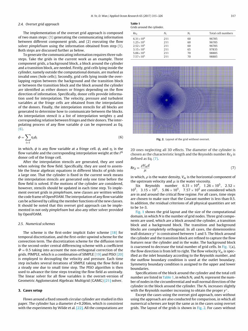
Table 1Grids around the cylinder.

Red Nc Nt Total cell numbers

6.31×104 211 60 967851.25×105 211 60 967852.52×105 211 60 967853.15×105 211 65 978355.06×105 211 70 988857.57×105 211 70 98885

H. Ye, D. Wan / Applied Oce

.4. Overset grid approach

The implementation of the overset grid approach is composedf two main steps: (1) generating the communicating informationetween different component grids, and (2) executing the flowolver pimpleFoam using the information obtained from step (1).oth steps are discussed further as below.

To generate the communicating information requires three sub-teps. Take the grids in the current work as an example. Threeomponent grids, a background block, a block around the cylindernd a transition block, are needed. Firstly, grid cells lying inside theylinder, namely outside the computational domain, are marked asnvalid ones (hole cells); Secondly, grid cells lying inside the over-apping region between the background and the transition blockr between the transition block and the block around the cylinderre identified as either donors or fringes depending on the flowirection of information. Specifically, donor cells provide informa-ion used for interpolation. The velocity, pressure and turbulentariables at the fringe cells are obtained from the interpolationf the donors. Finally, the interpolation stencils for all blocks areenerated to determine how to communicate between the blocks.n interpolation stencil is a list of interpolation weights andorresponding relation between fringes and their donors. The inter-olating process of any flow variable � can be expressed as Eq.6).

=∑i=1

i�i (6)

n which, � is any flow variable at a fringe cell. �i and i is theow variable and the corresponding interpolation weight at the ith

onor cell of the fringe cell.After the interpolation stencils are generated, they are used

hen solving the flow field. Specifically, they are used to assem-le the linear algebraic equations in different blocks of grids into

large one. That the cylinder is fixed in the current work meanshe interpolation stencils are generated only one time before theow field is solved. If the motions of the cylinder are considered,owever, stencils should be updated in each time step. To imple-ent overset grids in pimpleFoam, new classes are written within

he code frame of OpenFOAM. The interpolation of any flow variablean be achieved by calling the member functions of the new classes.t should be noted that this overset gird approach can be imple-

ented in not only pimpleFoam but also any other solver providedy OpenFOAM.

.5. Numerical schemes

The scheme is the first-order implicit Euler scheme [18] foremporal discretization, and the first-order upwind scheme for theonvection term. The discretization scheme for the diffusion terms the second-order central differencing scheme with a coefficient

= 0.5 taking into account the non-orthogonal correction of therids. PIMPLE, which is a combination of SIMPLE [19] and PISO [20]s employed to decoupling the velocity and pressure. Each timetep includes several iterations of SIMPLE taking the flow field as

steady one due to small time step. The PISO algorithm is thensed to advance the time steps treating the flow field as unsteady.he linear solver for all flow variables is the overset-version ofeometric Agglomerated Algebraic Multigrid (GAMG) [21] solver.

. Cases setup

Flows around a fixed smooth circular cylinder are studied in thisaper. The cylinder has a diameter d = 0.206m, which is consistentith the experiments by Wilde et al. [22]. All the computations are

Fig. 2. Layout of the grid without overset.

2D ones neglecting all 3D effects. The diameter of the cylinder ischosen as the characteristic length and the Reynolds number Red isdefined as Eq. (7).

Red = �Vind

�(7)

in which, � is the water density, Vin is the horizontal component ofthe upstream velocity and � is the water viscosity.

Six Reynolds number 6.31 × 104, 1.26 × 105, 2.52 ×105, 3.15 × 105, 5.06 × 105, 7.57 × 105 are considered whichare in and around the critical flow regime. For all cases, time stepsare chosen to make sure that the Courant number is less than 0.5.In addition, the residual criterions of all physical quantities are setto be 1e-3.

Fig. 1 shows the grid layout and the size of the computationaldomain, in which N is the number of grid nodes. Three grid compo-nents are used, which are a block around the cylinder, a transitionblock and a background block. The transition and backgroundblocks are completely orthogonal. In all cases, the dimensionlesswall distance y+ is constrained between 1 and 5. The block aroundthe cylinder and the transition block are refined to capture the flowfeatures near the cylinder and in the wake. The background blockis coarsened to decrease the total number of grid cells. In Fig. 1(a),the flow direction is from left to right. The flow velocity Vin is spec-ified as the inlet boundary according to the Reynolds number, andthe outflow boundary condition is used at the outlet boundary.Symmetry boundary condition is assigned to the upper and lowerboundaries.

Specifications of the block around the cylinder and the total cellnumber are listed in Table 1, in which Nc and Nt represent the num-ber of nodes in the circumferential and wall normal direction of thecylinder in the block around the cylinder. The Nt increases slightlywith the Reynolds number increasing to obtain the proper y+.

Except the cases using the overset gird approach, ones withoutusing the approach are also conducted for comparison, in which allnumerical schemes are kept the same as in the cases using oversetgrids. The layout of the grids is shown in Fig. 2. For cases without

318 H. Ye, D. Wan / Applied Ocean Research 65 (2017) 315–326

f resid

oao

Fig. 3. Time history o

verset grids, a grid convergence study is also carried out at first as spatial verification using 4 sets of grids. Due to space constraints,nly the final result that are used in this paper will be presented.

uals at different Red.

The result is obtained by using the third finest grid, in which Nc

and Nt are 270 and 102, respectively. The total cell number is 0.137million.

H. Ye, D. Wan / Applied Ocean Research 65 (2017) 315–326 319

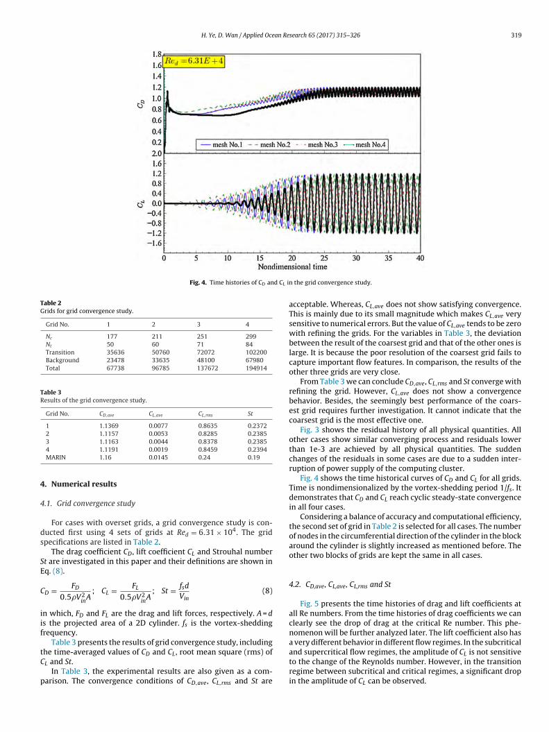
Fig. 4. Time histories of CD and CL in

Table 2Grids for grid convergence study.

Grid No. 1 2 3 4

Nc 177 211 251 299Nt 50 60 71 84Transition 35636 50760 72072 102200Background 23478 33635 48100 67980Total 67738 96785 137672 194914

Table 3Results of the grid convergence study.

Grid No. CD,ave CL,ave CL,rms St

1 1.1369 0.0077 0.8635 0.23722 1.1157 0.0053 0.8285 0.23853 1.1163 0.0044 0.8378 0.2385

4

4

ds

SE

C

iif

tC

p

4 1.1191 0.0019 0.8459 0.2394MARIN 1.16 0.0145 0.24 0.19

. Numerical results

.1. Grid convergence study

For cases with overset grids, a grid convergence study is con-ucted first using 4 sets of grids at Red = 6.31 × 104. The gridpecifications are listed in Table 2.

The drag coefficient CD, lift coefficient CL and Strouhal numbert are investigated in this paper and their definitions are shown inq. (8).

D = FD

0.5�V2in

A; CL = FL

0.5�V2in

A; St = fsd

Vin(8)

n which, FD and FL are the drag and lift forces, respectively. A = ds the projected area of a 2D cylinder. fs is the vortex-sheddingrequency.

Table 3 presents the results of grid convergence study, including

he time-averaged values of CD and CL , root mean square (rms) ofL and St.

In Table 3, the experimental results are also given as a com-arison. The convergence conditions of CD,ave, CL,rms and St are

the grid convergence study.

acceptable. Whereas, CL,ave does not show satisfying convergence.This is mainly due to its small magnitude which makes CL,ave verysensitive to numerical errors. But the value of CL,ave tends to be zerowith refining the grids. For the variables in Table 3, the deviationbetween the result of the coarsest grid and that of the other ones islarge. It is because the poor resolution of the coarsest grid fails tocapture important flow features. In comparison, the results of theother three grids are very close.

From Table 3 we can conclude CD,ave, CL,rms and St converge withrefining the grid. However, CL,ave does not show a convergencebehavior. Besides, the seemingly best performance of the coars-est grid requires further investigation. It cannot indicate that thecoarsest grid is the most effective one.

Fig. 3 shows the residual history of all physical quantities. Allother cases show similar converging process and residuals lowerthan 1e-3 are achieved by all physical quantities. The suddenchanges of the residuals in some cases are due to a sudden inter-ruption of power supply of the computing cluster.

Fig. 4 shows the time historical curves of CD and CL for all grids.Time is nondimensionalized by the vortex-shedding period 1/fs. Itdemonstrates that CD and CL reach cyclic steady-state convergencein all four cases.

Considering a balance of accuracy and computational efficiency,the second set of grid in Table 2 is selected for all cases. The numberof nodes in the circumferential direction of the cylinder in the blockaround the cylinder is slightly increased as mentioned before. Theother two blocks of grids are kept the same in all cases.

4.2. CD,ave, CL,ave, CL,rms and St

Fig. 5 presents the time histories of drag and lift coefficients atall Re numbers. From the time histories of drag coefficients we canclearly see the drop of drag at the critical Re number. This phe-nomenon will be further analyzed later. The lift coefficient also hasa very different behavior in different flow regimes. In the subcritical

and supercritical flow regimes, the amplitude of CL is not sensitiveto the change of the Reynolds number. However, in the transitionregime between subcritical and critical regimes, a significant dropin the amplitude of CL can be observed.

320 H. Ye, D. Wan / Applied Ocean Research 65 (2017) 315–326

Fig. 5. Time histories of CD and CL at different Red.

CL,ave,

coI

ipiA

Fig. 6. Comparisons of CD,ave,

Fig. 6 presents the results of different cases. We also conduct theomputations without overset grids. Computations with and with-ut overset grids are labeled as “overset” and “noOs”, respectively.n Fig. 6 are also experimental results by Wilde.

The range of Reynolds numbers covers the subcritical, crit-

cal and supercritical flow regimes. In Fig. 6(a), the drag-crisishenomenon (when Red reaches 3.0∼3.5 × 105) revealed by exper-

ments is not quantitatively predicted by the RANS simulation.lthough the RANS method averages the flow velocity, the decrease

CL,rms and St at different Red.

of drag can still be reflected from the change of mean flow veloc-ity. Moreover, numerical computations show that the SST model iscapable to capture flow separation to some degree [23–33]. But atthe same time, it may fail to predict where the separation starts.Both of these two reasons lead to results that current computa-

tions can only predict the trend of the drag-crisis but not predictquantitatively. The numerical results only capture a decreasingtrend of the drag in the critical regime. That “overset” and “noOs”obtain similar results indicates that the implementation of the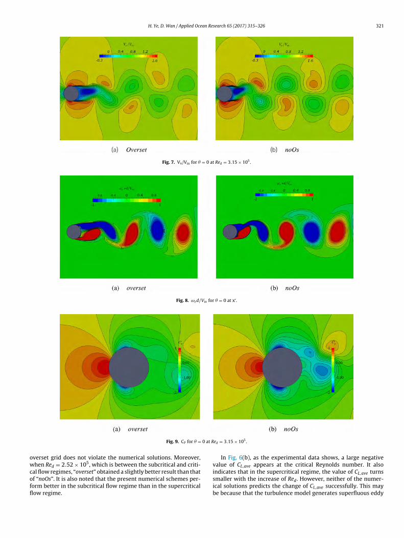

H. Ye, D. Wan / Applied Ocean Research 65 (2017) 315–326 321

Fig. 7. Vx/Vin for � = 0 at Red = 3.15 × 105.

Fig. 8. ωzd/Vin for � = 0 at x‘.

0 at R

owcoffl

Fig. 9. CP for � =

verset grid does not violate the numerical solutions. Moreover,hen Red = 2.52 × 105, which is between the subcritical and criti-

al flow regimes, “overset” obtained a slightly better result than that

f “noOs”. It is also noted that the present numerical schemes per-orm better in the subcritical flow regime than in the supercriticalow regime.

ed = 3.15 × 105.

In Fig. 6(b), as the experimental data shows, a large negativevalue of CL,ave appears at the critical Reynolds number. It alsoindicates that in the supercritical regime, the value of CL,ave turns

smaller with the increase of Red. However, neither of the numer-ical solutions predicts the change of CL,ave successfully. This maybe because that the turbulence model generates superfluous eddy

322 H. Ye, D. Wan / Applied Ocean Research 65 (2017) 315–326

for � =

vi

iesttRs

Fig. 10. Vx/Vin

iscosity dampening out some unsteadiness. Thus, it can furtherndicate that the k-ω SST turbulence model is dissipative.

The effect of instability of the separated shear layer in the crit-cal flow regime can also be observed in Fig. 6(c). According to thexperimental results, the intensity of the fluctuation of CL decreasesharply round the critical Reynolds number, and remains low inhe supercritical flow regime. The computational result captures

he downward trend but the magnitude is overestimated at alleynolds numbers. It should also be noted that “noOs” and “over-et” obtain similar results in the subcritical flow regime. The similar

0 by overset.

results indicate that the overestimation of CL,rms is not due to theimplementation of overset grids. In the supercritical flow regime,“overset” obtains better results than those of “noOs”. The large devi-ation between the results of “overset” and “noOs” at this Reynoldsnumber requires further investigations.

In Fig. 6(d), the computational result predicts St number with asatisfying accuracy in the subcritical flow regime. However, both

“overset” and “noOs” fail to predict both the sharp increase of Stnumber at the critical Reynolds number and its relatively largemagnitude in the supercritical regime. The discrepancy between

H. Ye, D. Wan / Applied Ocean Research 65 (2017) 315–326 323

for �

tti

oisatot

Fig. 11. ωzd/Vin

he results of “overset” and “noOs” is very limited, which justifieshat the implementation of overset grids does not have a negativenfluence on the prediction of St number.

In general, the implementation of overset grids does not deteri-rate the numerical accuracy or stability for all Reynolds numbersnvestigated in this paper. In the supercritical flow regime, the over-et grid approach slightly improved the results of CL,rms. It shouldlso be noted that the results of “noOs” and “overset” are close, but

he total cell number of “noOs” is about 1.4 times as large as thatf “overset”. It proves one advantage of the overset grid approachhat it can easily generate high quality grids with relatively less

= 0 by overset.

grid cells. Moreover, the overset gird approach combines with thenumerical schemes chosen in this paper has a satisfying accuracyfor predicting CD,ave, CL,ave and St in the subcritical flow regime. TheCL,rms predicted by “overset” are slightly better than those by “noOs”in the supercritical flow regime, but the CL,rms is still overall overes-timated at all Red. It is promising to use this overset grid approachtogether with more advanced turbulence models to predict the flowcharacteristics more accurately in the critical and supercritical flow

regimes.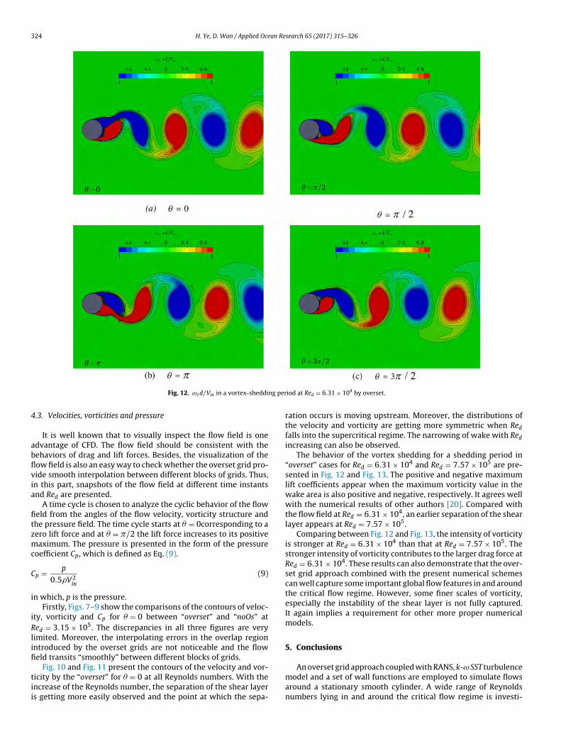

324 H. Ye, D. Wan / Applied Ocean Research 65 (2017) 315–326

ng per

4

abflvia

fitzmc

C

i

iRlifi

tii

Fig. 12. ωzd/Vin in a vortex-sheddi

.3. Velocities, vorticities and pressure

It is well known that to visually inspect the flow field is onedvantage of CFD. The flow field should be consistent with theehaviors of drag and lift forces. Besides, the visualization of theow field is also an easy way to check whether the overset grid pro-ide smooth interpolation between different blocks of grids. Thus,n this part, snapshots of the flow field at different time instantsnd Red are presented.

A time cycle is chosen to analyze the cyclic behavior of the floweld from the angles of the flow velocity, vorticity structure andhe pressure field. The time cycle starts at � = 0corresponding to aero lift force and at � = /2 the lift force increases to its positiveaximum. The pressure is presented in the form of the pressure

oefficient Cp, which is defined as Eq. (9).

p = p

0.5�V2in

(9)

n which, p is the pressure.Firstly, Figs. 7–9 show the comparisons of the contours of veloc-

ty, vorticity and Cp for � = 0 between “overset” and “noOs” ated = 3.15 × 105. The discrepancies in all three figures are very

imited. Moreover, the interpolating errors in the overlap regionntroduced by the overset grids are not noticeable and the floweld transits “smoothly” between different blocks of grids.

Fig. 10 and Fig. 11 present the contours of the velocity and vor-icity by the “overset” for � = 0 at all Reynolds numbers. With thencrease of the Reynolds number, the separation of the shear layers getting more easily observed and the point at which the sepa-

iod at Red = 6.31 × 104 by overset.

ration occurs is moving upstream. Moreover, the distributions ofthe velocity and vorticity are getting more symmetric when Red

falls into the supercritical regime. The narrowing of wake with Red

increasing can also be observed.The behavior of the vortex shedding for a shedding period in

“overset” cases for Red = 6.31 × 104 and Red = 7.57 × 105 are pre-sented in Fig. 12 and Fig. 13. The positive and negative maximumlift coefficients appear when the maximum vorticity value in thewake area is also positive and negative, respectively. It agrees wellwith the numerical results of other authors [20]. Compared withthe flow field at Red = 6.31 × 104, an earlier separation of the shearlayer appears at Red = 7.57 × 105.

Comparing between Fig. 12 and Fig. 13, the intensity of vorticityis stronger at Red = 6.31 × 104 than that at Red = 7.57 × 105. Thestronger intensity of vorticity contributes to the larger drag force atRed = 6.31 × 104. These results can also demonstrate that the over-set grid approach combined with the present numerical schemescan well capture some important global flow features in and aroundthe critical flow regime. However, some finer scales of vorticity,especially the instability of the shear layer is not fully captured.It again implies a requirement for other more proper numericalmodels.

5. Conclusions

An overset grid approach coupled with RANS, k-ω SST turbulencemodel and a set of wall functions are employed to simulate flowsaround a stationary smooth cylinder. A wide range of Reynoldsnumbers lying in and around the critical flow regime is investi-

H. Ye, D. Wan / Applied Ocean Research 65 (2017) 315–326 325

ng per

gard

1

2

3

4

5

Fig. 13. ωzd/Vin in a vortex-sheddi

ated. The numerical cases both with and without the overset gridpproach are carried out. From the comparisons among the presentesults and the experimental data, several conclusions are carefullyrawn:

. The results of the grid convergence study show that, the presentnumerical solutions are very sensitive to spatial resolution. Thecombination of the overset grid approach and pimpleFoam has asatisfying stability.

. As to CL,rms, the agreement between the results obtained from“overset” and the experiment data is satisfying in the supercrit-ical flow regime. However, a large discrepancy is noted in thesubcritical flow regime.

. The fluctuation of CL,ave is not captured by the present numericalresults, which may indicate that k-ω SST generates excess eddyviscosity.

. The results of drag force and St demonstrate that the presentnumerical schemes and models can predict some importanttrends in the critical flow regime, including the drag crisis and theincrease of St. However, the present numerical solutions fail toprovide an accurate quantitative prediction of the sharp changes.

. Important global flow features are captured by “overset”.Whereas, the present numerical solutions are incapable of pre-

dicting vorticities and instability of shear layers at a very finescale. This can directly cause that the flow characteristics in thecritical and supercritical flow regimes are not predicted quanti-tatively.

iod at Red = 7.57 × 105 by overset.

From the conclusions listed above, it can be seen that the presentrudimentary work demonstrates the accuracy, stability and effi-ciency of the overset grid approach. When the VIV problems arefurther studied, the quality of the overset grids will not degrade,since any block of the overset grids will not deform as conven-tional grids. Thus, the overset grid approach can be a more attractivechoice if the motions of a cylinder need to be considered. In addi-tion, a real riser usually has strikes making the geometric morecomplex, which can be easily handled by a set of overset grids.

The present results also expose the inefficiency of RANS com-bined with k-ω SST turbulence model and wall functions incapturing flow features in the critical flow regime. More advancedturbulence models or wall functions can be considered. In the cur-rent stage, to implement the overset grid approach with othernumerical models provided by OpenFOAM is available, but furtherverification and validation are still needed.

Acknowledgements

This work is supported by the National Natural Science Foun-dation of China (51379125, 51490675, 11432009, 51579145),Chang Jiang Scholars Program (T2014099), Program for Professorof Special Appointment (Eastern Scholar) at Shanghai Institutions

of Higher Learning (2013022) and Innovative Special Project ofNumerical Tank of Ministry of Industry and Information Technol-ogy of China (2016-23/09), to which the authors are most grateful.We also thank Prof. Pablo Carrica of University of Iowa for provid-

3 an Re

ip

R

[

[

[

[

[

[

[

[

[

[[

[

[

[

[

[

[

[

[

[

[

[

[

26 H. Ye, D. Wan / Applied Oce

ng the overset grid interpolating data which is an indispensableart of this work.

eferences

[1] A. Trim, H. Braaten, H. Lie, M. Tognarelli, Experimental investigation ofvortex-induced vibration of long marine risers, J. Fluids Struct. 21 (2005)335–361.

[2] G.N. Coleman, R.D. Sandberg. A primer on direct numerical simulation ofturbulence-methods procedures and guidelines, 2010.

[3] W. Rodi, Comparison of LES and RANS calculations of the flow around bluffbodies, J. Wind Eng. Ind. Aerodyn. 69 (1997) 55–75.

[4] C. Speziale, Turbulence modeling for time-dependent RANS and VLES: areview, AIAA J. 36 (1998) 173–184.

[5] S. Dong, G.E. Karniadakis, DNS of flow past a stationary and oscillatingcylinder at, J. Fluids Struct. 20 (2005) 519–531.

[6] P. Catalano, M. Wang, G. Iaccarino, P. Moin, Numerical simulation of the flowaround a circular cylinder at high Reynolds numbers, Int. J. Heat Fluid Flow 24(2003) 463–469.

[7] M. Saghafian, P. Stansby, M. Saidi, D. Apsley, Simulation of turbulent flowsaround a circular cylinder using nonlinear eddy-viscosity modelling: steadyand oscillatory ambient flows, J. Fluids Struct. 17 (2003) 1213–1236.

[8] E. Guilmineau, P. Queutey, Numerical simulation of vortex-induced vibrationof a circular cylinder with low mass-damping in a turbulent flow, J. FluidsStruct. 19 (2004) 449–466.

[9] Z. Pan, W. Cui, Q. Miao, Numerical simulation of vortex-induced vibration of acircular cylinder at low mass-damping using RANS code, J. Fluids Struct. 23(2007) 23–37.

10] A. Travin, M. Shur, M. Strelets, P. Spalart, Detached-eddy simulations past acircular cylinder flow, Turbul. Combust. 63 (2000) 293–313.

11] P.M. Carrica, R.V. Wilson, R.W. Noack, F. Stern, Ship motions usingsingle-phase level set with dynamic overset grids, Comput. Fluids 36 (2007)1415–1433.

12] W.D. Henshaw, Overture: an object-oriented framework for overlapping gridapplications, AIAA Conference on Applied Aerodynamics (2002).

13] Z. Shen, D.C. Wan, P. Carrica, Dynamic overset grids in OpenFOAM withapplication to KCS self-propulsion and maneuvering, Ocean Eng. 108 (2015)287–306.

14] D.C. Wan, Z. Shen, Overset-RANS computations of two surface ships moving

in viscous fluids, Int. J. Comput. Methods 9 (2012) 1–14, 1240013.

15] F.R. Menter, Two-equation eddy-viscosity turbulence models for engineeringapplications, AIAA J. 32 (1994) 1598–1605.

16] D.C. Wilcox, Turbulence Modeling for CFD, DCW industries, La Canada, CA,1998.

[

search 65 (2017) 315–326

17] I. Rodríguez, O. Lehmkuhl, J. Chiva, R. Borrell, A. Oliva, On the flow past acircular cylinder from critical to super-critical Reynolds numbers: waketopology and vortex shedding, Int. J. Heat Fluid Flow 55 (2015) 91–103.

18] H. Jasak. Error analysis and estimation for the finite volume method withapplications to fluid flows. 1996.

19] S. Patankar, Numerical Heat Transfer and Fluid Flow, CRC Press, 1980.20] R.I. Issa, Solution of the implicitly discretised fluid flow equations by

operator-splitting, J. Comput. Phys. 62 (1986) 40–65.21] J.H. Ferziger, M. Peric, Computational Methods for Fluid Dynamics, Springer

Science & Business Media, 2012.22] J. De Wilde, R. Huijsmans, Experiments for high Reynolds numbers VIV on

risers international society of offshore and polar engineers, The EleventhInternational Offshore and Polar Engineering Conference (2001).

23] E. Furbo, J. Harju, H. Nilsson. Evaluation of turbulence models for prediction offlow separation at a smooth surface Unpublished, 2009.

24] Z. Shen, H. Ye, D.C. Wan, URANS simulations of ship motion responses inlong-crest irregular waves, J. Hydrodyn. 26 (3) (2014) 436–446.

25] R. Zha, H. Ye, Z. Shen, D.C. Wan, Numerical computations of resistance of highspeed catamaran in calm water, J. Hydrodyn. 26 (6) (2014) 930–938.

26] H. Cao, D.C. Wan, RANS-VOF solver for solitary wave run-up on a circularcylinder, China Ocean Eng. 29 (2) (2015) 183–196.

27] W. Zhao, D.C. Wan, Numerical investigation of vortex-Induced motions ofSPAR platform based on large eddy simulation, Chin. J. Hydrodyn. 30 (1)(2015) 40–46.

28] Z. Shen, D.C. Wan, An irregular wave generating approach based onnaoe-FOAM-SJTU solver, China Ocean Eng. 30 (2) (2016) 177–192.

29] W. Zhao, D.C. Wan, Numerical study of 3D flow past a circular cylinder atsubcritical reynolds number using SST-DES and SST-URANS, Chin. J.Hydrodyn. 31 (1) (2016) 1–8.

30] W. Zhao, D.C. Wan, R. Sun, Detached-eddy simulation of flows over a circularcylinder at high reynolds number, proceedings of the twenty-sixth (2016), in:International Ocean and Polar Engineering Conference Rhodes, Greece June26–July 1, 2016, pp. 1074–1079.

31] W. Zhao, D.C. Wan, Numerical computations of spar vortex-Induced motionsat different current headings, in: Proceedings of the Twenty-sixth (2016)International Ocean and Polar Engineering Conference Rhodes, Greece June26–July 1, 2016, pp. 1122–1127.

32] M. Duan, D.C. Wan, Frequency and moving direction effects on lift, drag andvortex mode for flows around an oscillating cylinder, in: Proceedings of theTwenty-fifth (2015) International Ocean and Polar Engineering Conference,

Kona, Big Island, Hawaii, USA, June 21–26, 2015, pp. 1010–1017.

33] M. Duan, D.C. Wan, H. Xue, Prediction of response for vortex-inducedvibrations of a flexible riser pipe by using multi-strip method, in: Proceedingsof the Twenty-sixth (2016) International Ocean and Polar EngineeringConference Rhodes, Greece June 26–July 1, 2016, pp. 1065–1073.