Applied Differential Geometry - sam.math.ethz.chhiptmair/Courses/CEM/BOS02c.pdf · Applied...

©A. Bossavit, 1994-2002. Last update: May 2002

Applied Differential Geometry (A compendium)

The content of these notes is what "compendium" suggests: Not a tutorial, but alist, in logical order, of concepts of differential geometry that can serve in thestudy of PDE's of classical physics, each with a condensed description1. Theidea is to guide the reader along a way that can, for one who wants to reach thosespots most useful for applications, be faster than conventional courses. But theneed for a reference book will probably be felt. Good books about differentialgeometry, "pure" or "applied", exist in abundance, and the bibliography listssome. Select a few for yourself, and use what follows as a check-list to guide yourstudy. Don't worry too much about mathematical technique as such (there arerelatively few subtle or difficult proofs2 in the subject, in comparison with itsrichness in concepts and structures), and try to gain geometric intuition.

Italics, besides their use for emphasis, serve here to highlight a word whichis being defined, explicitly or implicitly. When a function f maps all or part ofX into Y, we'll say that f is "of type X → Y", and denote by dom(f) the subset ofX formed of points for which f(x) makes sense, or domain of f. The codomainf(x) : x ∈ X will be cod(f). If a function f is defined by some formula orexpression, such as x → Expr(x), we shall feel authorized to write "f = x →Expr(x)", thus defining the left side by the right side. Then, both sides of thisequality point to the same object, the function f. Ck means "differentiable ktimes", C0 means "continuous", C∞ means "differentiable ad libitum". Its synonym"smooth" can at places be understood as "differentiable as many times as requiredby the situation" (a cop-up for sure, but so convenient). Symbols may be overloaded,with context-dependent meaning.

0. AFFINE PRELIMINARIESAffine space. You know what a vector space is. The real n-dimensional vectorspace will be denoted Vn in what follows. Affine space is "what is left of Vnwhen the origin is ignored". More seriously, affine space An is a set of points onwhich Vn acts by translations: This means that to each v of Vn is associated atransform x → Tvx of An to itself, the translation by v, with Tv(Twx) = Tv + w x;

1 Not always proper definitions, however. Some fine points are glossed over. There is some risk in this,but the approach to applicable differentiable geometry can too easily be slowed down by excessivefussiness.2 Most proofs are terse one- or two-liners, inserted between brackets as a warning that you shouldrather redo them yourself.

moreover, one requires that Tvx = x iff v = 0 and that for each y there be a v

2 APPLIED DIFFERENTIAL GEOMETRY

such that y = Tv x. It's convenient, for obvious reasons, to denote this v by y – x,and Tv x by v + x.

The other way round, start from an affine space A, select a point o to playthe role of origin, and the "translation vectors" x – o form a vector space, associatedw i t h A. The dimension of A is defined as that of V.Barycenter. Given x, y, and a real θ, this is (1 – θ)x + θy, that is, T θvx, where v =y – x. This generalizes to k points, hence the notions of a f f ine basis, a f f inesubspace, barycentric coordinates (for k = n + 1). We shall indulge in writing x =∑i = 0, ..., n λ

i(x) xi, where what is meant is the vector equality ∑i λi(x) (xi – x) = 0.

Affine space makes a better framework than vector space for elementaryclassical physics. Unless some point cries out to be taken as origin, as may happenin celestial mechanics for instance, there is really no reason to distinguish one,and to work with vectors when points do just fine. So one should be careful not tosay "vector" where "point" is implied, and to distinguish "components" (of vectors)from "coordinates" (of points). Don't confuse IRn with Vn either.

1. DIFFERENTIABLE MANIFOLDS

Manifolds. These are topological spaces that "look, locally, like An": A curve (n= 1), a surface (n = 2), the configuration space of a solid (n = 6), etc. Another wayto describe them is as "patchworks of pieces of An, smoothly sewn up". Withmore precision, one is given a set of maps ϕα, α ∈ A, also called "charts", of typeX → IRn (the integer n is the dimension of X), each of which maps a part of Xonto a domain of IRn, bijectively. The set-union of the domains dom(ϕα) should beX, and the ϕα ϕβ

–1 should be C∞ for all pairs α, β (compatibil ity condition ofcharts). Each chart maps a part of X onto a piece of IRn, thus providing a systemof "local coordinates" on X, and its inverse is a "local parameterization" of X.The idea is to provide sets with a structure that allows to do on them all that canbe done in standard differential calculus. Thus, for instance, a function f of typeX → IR is deemed C∞ at x if the composition f ϕ−1 is C∞ , for some chart ϕ thedomain of which covers x. If this property holds for a chart, it holds for anycompatible chart: the compatibility condition is there to enforce this.

A set of charts is called an a t l a s. There may be few charts in an atlas (as fewas two, for instance, may be enough to cover a sphere, if chosen well), but one mayinclude as many of them as required by convenience in a descriptive atlas. The setof a l l charts compatible two by two with the given ones is the complete atlas."The" manifold should be conceived as the structure formed by X and the completeatlas. (Be aware that the same set can conceivably be provided with two different,non-compatible complete atlases. But in that case, of course, one has two differentmanifolds. )Manifolds w i t h boundary. Same thing, but this time there are points (those ofthe boundary) where X looks locally like the half-space x ∈ IRn : x1 ≥ 0. Theboundary forms by itself a manifold (the boundary of which is empty), of dimensionn – 1, denoted ∂X. From now on, "manifold" should be understood as "manifoldwith boundary", the boundaryless ones defined above being a subcategory.3

1. DIFFERENTIABLE MANIFOLDS 3

Tangent vectors at x ∈ X, called "vectors at x". These are equivalence classes oftrajectories passing through x. Such a trajectory is a smooth map g : IR → X suchthat g(0) = x (smooth, in line with our above conventions, means that t → ϕ(g(t))is C∞ for any chart ϕ covering x). Two trajectories g and g' are equivalent if|ϕ(g(t)) − ϕ(g'(t))| = o(t), which intuitively means they are tangent and velocitiesat time 0 match. One will check that this equivalence is, like the smoothness ofg and g', a chart-independent fact (again, the compatibility relation betweencharts does this). Tangent vectors can thus be understood as velocity vectors, butbeware there is no pre-existing affine space in which the trajectory is inscribed,hence no preexisting vector space the tangent vector is an element of. The tangentvector i s the equivalence class.Tangent space at x. Denoted TxX, it's the set of all tangent vectors at point x,according to the above definition. It's isomorphic to Vn, the n-dimensional realvector space. Its structure of linear space comes from Vn via ϕ, and this structuredoes not depend on which chart is considered.Tangent m a p at x. A smooth mapping u ∈ X → Y, with dom(u) open in X,transforms trajectories at x ∈ X into trajectories at y = u(x) in Y, and hencevectors of Tx X into vectors of TyY. The correspondence of type Tx X → TyY thusestablished is linear and is usually denoted u*(x). If v is a vector at x, the vectoru*(x)v at y = u(v) is dubbed its push-forward.Immersions. Smooth maps, which may not be one-to-one, but the tangent maps ofwhich have maximal rank. For instance, (a) to (d) in Fig. 1.1 are immersions, and(e) is not. The latter may very well be smooth, that is, C∞ from IR to IR2, in spiteof not looking that way (think of the projection of a smooth spatial curve alongone of its tangents), but the tangent map at the tip of the cusp is two-to-one.(Another example would be: a trajectory without cross-overs, but with a vanishingspeed at some point—but this is harder to render graphically.)

a b c ed

FIGURE 1.1. Five mappings of IR (or as well, the open segment ]0, 1[) as X, into IR2 as Y.Only (a) qualifies as an embedding, even though (b) is a bijective immersion (end-points arenot in the image). Maps (b), (c) and (d) are immersions, but not (e). One may legitimatelyconceive doubts about (d), but observe that a restriction to a small enough subinterval ]α, β[of ]0, 1[ is an embedding, in case (d) as well as in cases (b) or (c). Case (d) looks specialbecause it's not a "generic position" immersion: slightly moving the curve will either suppressthe first-order contact or create two frank intersections, like the one in (c). The only submanifoldof the plane, in this picture, is under (a).

Diffeomorphisms. Bijective C∞ maps from one manifold onto another, that is,maps which preserve the structure of differentiable manifold. Two diffeomorphic

3 An open disk in IR2, for instance, has the structure of a two-dimensional manifold, but one whoseboundary is empty (just like IR2, to which it is diffeomorphic). But this manifold is implicitly describedas embedded in IR2, where its image has a non-empty topological boundary.

manifolds have the same dimension.


Embedding. A one-to-one mapping u : Y → X which is already an immersion andconstitutes a diffeomorphism between Y and u(Y). (Conversely, an immersion islocally an embedding, i.e., reduces to one by restriction to a part of Y.) One thensays that u(Y) is a submanifold of X (and confuses Y with u(Y) if no hazardensues). Figure 1.1 gives an example and four counter-examples.4

If Y is embedded in X, the tangent space TxY at x ∈ Y, being abstractedfrom trajectories inscribed in Y, can be identified with a subspace of TxX. Tangentvectors at x not contained in TxY are said transverse to Y.

In particular, Tx∂X is a subspace of codimension 1 inside Tx X. Vectors of Tx Xwhich are transverse to ∂X can be classified, in an obvious way, as outward orinward transverse vectors.Remark. Immersion is a useful notion, because some manifolds of dimension 2,quite easily described via charts, cannot be embedded in three-dimensional space,but can still be immersed, which helps visualize them. For instance, Fig. 1.2shows how to define two (boundaryless) manifolds of dimension 2, the torus andthe Klein bottle, together with immersions of them (which as regards the torus ishere, but need not be, an embedding). One can reason on the upper figures, but theother two are more lively. ◊

a cb

b c

a

c

b

b

a

aa

c

ba

cb

a

aa

c

a

a

cb

a

aa

c

FIGURE 1.2. Torus, Klein bottle and projective plane as "abstract" manifolds and as immersedin 3D space. (Can you supply the missing drawing?) Starting from a manifold with boundary,one identifies the edges as suggested. Charts are equally easy to devise in all cases.(Neighborhoods of a, b and c are suggested.) But finding an immersion for the projectiveplane is quite a task, a book-size subject [Ap, Br, Co, Fr].

Basis vectors at a point, relative to a chart ϕ. Consider the trajectories γ i = t →ϕ(x) + 0, ..., t, ...,0 ∈ IRn, with t in ith position: Thus, γ i is a straight line,containing ϕ(x), parallel to the ith coordinate axis in IRn, ran along at speed 1.Now consider the trajectories gi = t → ϕ−1(γ i(t)), which are inverse images under ϕof the γ is. The gis are the coordinate lines on X, containing x. The basis vectorsat x are, by definition, their equivalence classes. One denotes them by ∂i(x), i =1, ..., n. (Why "∂", among all symbols, will soon be clear.) They form vector

4 Embedding is a delicate notion, a case of "monster-barring" in the sense of Lakatos [La]. The idea is,as always, to avoid pathological situations without sacrificing generality. Close examination of texts byreputable authors like, on the one hand, [KN] or [EDM], on the other hand, [RF] or [Ar], or ['N] (whichI follow here, cf. p. 19) will show them in slight disagreement on what an embedding exactly is.

fields (see below) x → ∂i(x), denoted ∂i. These are only locally defined, that is,


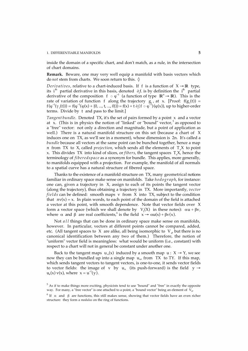
inside the domain of a specific chart, and don't match, as a rule, in the intersectionof chart domains.Remark. Beware, one may very well equip a manifold with basis vectors whichdo not stem from charts. We soon return to this. ◊Derivatives, relative to a chart-induced basis. If f is a function of X → IR type,its i th partial derivative in this basis, denoted ∂if. is by definition the ith partialderivative of the composition f ϕ−1 (a function of type IRn → IR). This is therate of variation of function f along the trajectory gi , at x. [Proof: f(g i(t)) =f (ϕ−1(γ i(t))) = f(ϕ−1(ϕ(x) + 0, ..., t, ..., 0)) = f(x) + t ∂i( f ϕ−1) (ϕ(x)), up to higher-orderterms. Divide by t and pass to the limit.]Tangent bundle. Denoted TX, it's the set of pairs formed by a point x and a vectorat x. (This is in physics the notion of "linked" or "bound" vector, 5 as opposed toa "free" vector: not only a direction and magnitude, but a point of application aswell.) There is a natural manifold structure on this set (because a chart of Xinduces one on TX, as we'll see in a moment), whose dimension is 2n. It's called abundle because all vectors at the same point can be bunched together, hence a mapπ from TX to X, called projection, which sends all the elements of TxX to pointx. This divides TX into kind of slices, or fibers, the tangent spaces TxX, hence theterminology of f ibered space as a synonym for bundle. This applies, more generally,to manifolds equipped with a projection. For example, the manifold of all normalsto a spatial curve has a natural structure of fibered space.

Thanks to the existence of a manifold structure on TX, many geometrical notionsfamiliar in ordinary space make sense on manifolds. Take hodograph, for instance:one can, given a trajectory in X, assign to each of its points the tangent vector(along the trajectory), thus obtaining a trajectory in TX. More importantly, vectorf i e lds can be defined: smooth maps v from X into TX, subject to the conditionthat πv(x) = x. In plain words, to each point of the domain of the field is attacheda vector at this point, with smooth dependence. Note that vector fields over Xform a vector space (which we shall denote by V1(X) in these notes): αu + βv,where α and β are real coefficients,6 is the field x → αu(x) + βv(x).

Not a l l things that can be done in ordinary space make sense on manifolds,however. In particular, vectors at different points cannot be compared, added,etc. (All tangent spaces to X are alike, all being isomorphic to Vn, but there is nocanonical identification between any two of them.) Therefore, the notion of"uniform" vector field is meaningless: what would be uniform (i.e., constant) withrespect to a chart will not in general be constant under another one.

Back to the tangent maps u*(x) induced by a smooth map u : X → Y, we seenow they can be bundled up into a single map u*, from TX to TY. If this map,which sends tangent vectors to tangent vectors, is one-to-one, it sends vector fieldsto vector fields: the image of v by u* (its push-forward) is the field y →

5 As if to make things more exciting, physicists tend to use "bound" and "free" in exactly the oppositeway. For many, a "free vector" is one attached to a point, a "bound vector" being an element of Vn.6 If α and β are functions, this still makes sense, showing that vector fields have an even richerstructure: they form a modulus on the ring of functions.

u*(x) v(x), where x = u–1(y).


Frame. A f rame at x is a basis for Tx X, that is, a system of n linearly independentvectors. A l oca l frame in a neighborhood of x is a locally defined field of frames,that is to say, a system of n smooth vector fields w1, ..., wn, such that thecorresponding vectors at x be independent, for all x in the intersection of thedomains of each wi. A frame is global if dom(wi) is all of X, for all i. One canalways find a local frame about a point. For instance, the above basis vectorsmake one, the basis vector fields, denoted ∂ i, being defined by ∂i = x → ∂i(x). (Thedomain dom(∂i) is the domain of the defining local chart.) But no global frameexists, in general. On the surface of a sphere, for example, none can be devised.Components. Given a local frame wi : i = 1, ..., n, a vector field v can bewritten, still locally, as v = x → ∑ i = 1, ..., n v

i(x) wi(x), or in abridged form, v =∑i v

i wi. The real numbers v i are the components of v, relative to this frame. Ifthe local frame is made of the chart-induced ∂ is, one has v = ∑i v

i ∂i, and the v isare the components of v relative to this chart.Holonomy. This property7 of a local frame that one can find a local chart the∂i's of which are the frame vectors. A given local frame has no reason to beholonomic [Ca], as soon as dimension exceeds two. Most of those encountered inpractice, however, are. (See below what makes them so.)Vector fields as differential operators. A vector field v can be seen as adifferentiation: Indeed, if f is a smooth real-valued function on X, its rate ofvariation along one of the trajectories of class v is ∑ i v

i ∂if [an easy computation:f(g(t)) = f(ϕ−1(γ i(t))) = f(ϕ−1(ϕ(x) + tv1, ..., vi, ..., vn)) = f(x) + t ∑i v

i ∂i( f ϕ−1) (ϕ(x)),up to higher-order terms], and this can be read as (∑ i v

i ∂i) f, that is, as the effecton f of a derivation operator. So why not write that "v f" ? Replace v by ∂ i,now, and both interpretations of "∂ if" appear to be in harmony. Hence the use ofthe differentiation symbol ∂ i to denote the i-th chart-induced basis vector field.The other way round, a derivation, that is, a linear operation ∂ of type C∞(X) →C∞(X) that maps constants to 0 and obeys Leibniz's rule, ∂(fg) = ∂f g + f ∂g,corresponds to the vector field ∑i ∂ϕ

i ∂i, where ϕ is the chart (cf. [2], p. 83).Lie bracket. Given two vector fields u and v, should we expect that uvf = vuf? Ifu = ∂ i and v = ∂ j, so is the case (∂i∂j f = ∂ j∂i f, denoted ∂ ijf, by the classical Schwarzequality), but otherwise, uvf = (∑i u

i ∂i) (∑j vj ∂j)f = ∑ ij u

i vj ∂ ij f + ∑ ij ui ∂i v

j ∂j f, and( uv – vu)f = ∑ ij u

i ∂i vj ∂j f – ∑ij u

i ∂i vj ∂j f = ∑j (u vj – v u j) ∂ j f, which has no reason to

vanish. The vector field ∑j (u v j – v uj) ∂ j is called the Lie bracket of u and v,denoted [u, v]. The Jacobi identity

[[u, v], w] + [[v, w], u] + [[w, u], v] = 0

is easily verified. (Whoever knows how to park a car along a kerb has intuitivegrasp of the Lie bracket; see [30], p. 234.)

7 Again, be wary of the frequent use of this word, as criticized, e.g., in [Be], to mean the contrary, thatis anholonomy — lack of holonomy. The relevant geometric object, a group, which happens to be trivialin case of holonomy, should thus be called "anholonomy group". Needless to say, it's holonomy groupthat is in use, and there is little hope for reconciliation between the two schools.8 The concept of Lie bracket applies to vector fields, not to vectors.

We may now observe8 that [∂ i, ∂j] = 0. A given local frame w i : i = 1, ..., n is


holonomic, one may prove (cf. [25], p. 47), if all Lie brackets [wi, wj] vanish.Lie algebra. A vector space V equipped with an anti-commutative bilinearoperation [ , ] : V × V → V such that Jacobi's identity holds. Examples: Ordinary3D Euclidean space (see below), with [v, w] = v × w; The vector space of n × nmatrices, with [A, B] = AB – BA.

The vector space V1(X) of smooth vector fields over X (or more generally,V1(O), where O is an open set of X), is thus a Lie algebra. It's often of interest toknow whether a family of vector fields, which make a subspace of V1(X), alsomake a Lie algebra, that is, whether [u, v] always belongs to the family when uand v do. One then has a Lie subalgebra. For instance, the fields α∂1 + β∂2, withconstant (beware!) coefficients α and β, form a Lie subalgebra of V1(dom(ϕ)) .Covector. An element of the dual (denoted Tx*X) of TxX. The duality productbetween the covector ω and vector v (i.e., the "effect" of one on the other) iswritten <ω ; v>. If there is at x a basis ∂i : i = 1, ..., n of vectors (x understood),there is also a so-called "dual" basis of covectors: these are the linear maps di :Tx X → IR (x understood) defined9 by <di , ∂ j > = 1 if i = j, else 0. Setω i = <ω ; ∂i> . Then <ω ; v> = ∑i ω i v

i, so one can expand ω as ω = ∑ i ω i di in the

dual basis, and one has <ω ; v> = ∑i ω i vi.

Cotangent bundle. The manifold of dimension 2n, denoted T*X, composed of thecovectors. We just saw how to get a local map.

If u maps X to Y, how covectors behave with respect to u is a naturalquestion. Given η in Ty*Y, where y = u(x), its pull-back u*(x)η is the covector atx such that <u*(x)η ; v>X = <η ; u*(x)v>Y for all v in TxX.p-covector at x. Maps of type Tx X × ... × Tx X → IR, with p factors on the left ofthe arrow, which are linear with respect to all factors, and alternating, that is,the permutation of two factors reverses the sign of the result. The effect is denoted<ω ; vI, ..., vp> . Determinants and their minors are a familiar example. If acovector basis di : i = 1, ..., n exists at x, there is also a basis for p-covectors,the elements of which, denoted10 dσ(1) ∧ dσ(2) ∧ ... ∧ dσ(p), are obtained by taking allincreasing injections σ from the integer segment [1, p] to [1, n]. By definition, theeffect of the previous covector on a set of p vectors v1, v2, ..., vp is

(1.1) <dσ(1) ∧ dσ(2) ∧ ... ∧ dσ(p) ; v1, v2, ..., vp>

= ∑ π v1σ ο π (1) v2

σ ο π(2) ... vpσ ο π(p) sign(π)

where π spans the set of all permutations of [1, p], and sign(π) denotes the

9 The notation d i is an innovation. I believe it's more logical than the received one, that would bedxi, as found in such expressions as dx1 ∧ dx2 ∧ ... ∧ dxn, or in low dimension, dx ∧ dy, dx ∧ dy ∧ dz,etc. See the section on Integration for the relation between "differential elements" like dx, etc., andcovectors. The advantages of d i are so obvious that I hope this will catch. (I've been hoping for nowten years.)10 The use of σ (and, below, ς) is also a new proposal. A long familiarity with "old tensor" notationhas led to undue indulgence for atrocious displays like dxi1 ∧ dxi2

∧ ... ∧ dxin , with indexation of

unlimited depth, the meaning of which gets clarified only by explicitly introducing the mapping σ(then i1 is recognized as σ(1), etc.).

signature of π. Thus, for instance, <d 1 ∧ d2 ; v, w> = v 1 w 2 − v2 w 1. There are as


many p-covectors in the basis as ways to select p objects among a family of n,order being meaningful (combinations p by p). So there is a single basis p-covectorif p = 0 or n. For p = 0, it's by convention the real number 1, and for p = n, thedeterminant of the matrix of components of the n factors according to the chart ϕ.We'll denote by Fx

p the space of p-covectors at x. Each Fxp, for x fixed, is

isomorphic to the linear space, often denoted Λp, of alternating p-linear formson Vn. By convention, a 0-covectro is just a real number, and Λ0 = R.

In presence of u : X → Y, the pull-back of a p-vector η at y = u(x) is definedby <u*(x)η ; vI, ..., vp>X = <η ; u*(x)v1, ..., u*(x)vp>Y for all v1, ..., vp in TxX.

For two integers p and q, consider an increasing injection σ from the integersegment [1, p] into [1, p + q]. One will denote by ς the increasing injection from[1, q] into [1, p + q] which "complements" σ, uniquely determined by the conditionς(i) ≠ σ(j) ∀ i, j. The signature of the permutation i → i f i ≤ p then σ(i) elseς(i − p) will be denoted sign(σ, ς). The set of all possible σ (isomorphic to theset of combinations of p objects chosen among p + q) will be denoted11 C (p, q).Exercise. Generalize to p = 0, or q = 0, or both. Generalize to complementaryinjections from [k + 1, k + p] and [l + 1, l +q] into [m, m + p + q – 1], where k, l,and m can be any relative integers.Exterior product (aka wedge product). The exterior product of a p-covector ωand a q-covector η (both at the same point x) is the (p + q)-covector defined by

<ω ∧ η ; v1, ..., vp, vp + 1, ..., vp + q> =

(1.2) ∑ σ ∈ C (p, q) <ω ; vσ (1), ..., vσ(p)> <η ; vς (1), ..., vς (q)> sign(σ, ς) .

(It i s a covector: If two vis are equal, the same term will appear twice in (12)with opposite signatures.) This operation is associative, and one will check that(1.1) above was indeed the exterior product of the basis covectors dσ(i), whichjustifies the use of ∧ in (1.1). Wedge product is not commutative, but anti-commutative, in the following sense:

(1.3) η ∧ ω = (−1)pq ω ∧ η.

Wedge and pull-back go along naturally: u*(ω ∧ η) = u*ω ∧ u*η, as easilyestablished from (1.2) and the definition of u*. Note that ω ∧ η = 0 if p + qexceeds n, the ambient dimension,Exercise. Can ω ∧ ω be nonzero?Inner product. To a p-covector ω , p ≥ 1, and a vector v, this operation associatesthe (p – 1)-covector

i vω = v2, ..., vp → <ω ; v, v2, ..., vp>

(also denoted v ω by some, cf. e.g. [Bu]). In particular, when p = 1, ivω is just< ω ; v>. About the interaction with pull-back, iv(u*ω ) = u*[iu*v

ω ], that is

(1.4) ivu* = u*iu*v

11 This is in the spirit of H. Cartan, who favored the symmetric notation (p, q) for the binomialcoefficient which gives the number of p-by-b combinations of p + q objects (cf. [HP], p. 159).


and ivu* = u*iv when v is invariant, u*v = v, a remark we'll use later. Wedge andi relate like this, after (1.2):

(1.5) iv(ω ∧ η) = ivω ∧ η + (–1)p ω ∧ ivη,

where p is the degree of ω . [Proof: Let v1 = v. Permutations σ fall into twoclasses, those for which σ(1) = 1, those for which ς(1) = 1. Observe how thisinduces complementary injections from [2, p] and [1, q] (in the former case) orfrom [1, p] and [2, q] (in the latter case) into [2, n], and how the signature ofthese relates with sign(σ, ς). (They are the same if σ(1) = 1, differ by the sign of(–1)p if ς(1) = 1.) Split the right-hand side of (1.2) accordingly, into two sums.one of which appears to be ivω ∧ η and the other one (–1)p ω ∧ i vη.]Exercise. Show that iv iv = 0.Exercise. When can ivω ∧ ω be nonzero?Multivectors. These are the dual objects, a p-vector being an element of the dualof Λp, a bound p-vector at x, an element of the dual of Fx

p. Basis p-vectors∂σ(1) ∨ ∂σ(2) ∨ ... ∨ ∂σ(p) can be defined by the formula

<dσ(1) ∧ dσ(2) ∧ ... ∧ dσ(p), ∂σ(1) ∨ ∂σ(2) ∨ ... ∨ ∂σ(p)> = 1

(and 0 if indices don't match at they do here, – 1 if they do up to an oddpermutation). In coordinates, the generic field of p-vectors is

x → ∑ σ ∈ C (p, n – p) vσ(x) ∂σ(1) ∨ ∂σ(2) ∨ ... ∨ ∂σ(p).

The "join" ∨ thus introduced behaves like12 the "wedge" ∧ : just use (1.2),exchanging vectors and covectors. It goes along with push-forward: u*(v ∨ w) =u*v ∨ u*w.

A "simple" bivector such as v ∨ w can be visualized as the orientedparallelogram built on v and w, and since v ∨ w = v ∨ (w + λv), as any otherparallelogram of equal area13 in this plane, and while we are at it, as any pieceof the plane of equal algebraic area.14 Such a bivector "is" therefore, an equivalenceclass of figures in a plane, characterized by a common (positive or negative) area,just as a vector is the class of segments of same algebraic length on a given line.Not all bivectors are of this kind, in general, but so is the case in dimension 3: Abivector α ∂y ∨ ∂z + β ∂ z ∨ ∂x + γ ∂ x ∨ ∂y can be represented by the join of twovectors. Trivectors (and n-vectors, in dimension n), also have easy geometricinterpretation: equivalence classes of figures of equal volume.Differential form of degree p: A C∞ field of p-covectors, or p-form. One willdenote by F p (X) the collection of all p-forms on X. (It's more than a vectorspace, it's a modulus on the ring of functions, cf. Note 6.) Differential forms of

12 Rota [B&] makes a convincing case for the use of ∨ in this context. One more often sees ∧ there.13 Area is a metric concept (see below), but ratio of areas, in a given plane, is a purely affine notion(take the obvious determinant).14 There is a popular interpretation of bivectors as rotations in the support plane ([Hs], p. 1020). Thisrequires a metric, however, a fact that fans of this "geometric algebra" approach tend to downplay.

degree 0, or 0-forms, are the smooth functions of type X → IR, or scalar f i e lds . In


a local chart, a p-form can be written as

ω = x → ∑ σ ∈ C (p, n – p) ωσ(x) dσ(1) ∧ dσ(2) ∧ ... ∧ dσ(p),

where the coefficients ωσ are C∞ functions. The dual concept, a field of p-vectors,is less popular, and has no universally recognized name. (Such fields form a spaceVp(X); we already met with V1(X).)

In particular, the generic 1-form is ω = x → ∑ i = 1, ..., n ω i(x) di(x). By linearityof ω , one has <ω ; v> = ∑ i ω i v

i (with x understood), as one would expect. A fulldevelopment of such coordinate-dependent computational techniques would leadto a brief on tensor calculus. Let's just mention the popular Einstein conventionabout implicit summation (not followed here), that consists in omitting the ∑ inexpressions such as ∑ i ω i d

i, where the summation index appears both as a subscriptand a superscript.

In presence of a map u : X → Y, the pull-back of a p- form η, living on Y, isthe p-form x → u*(x)η(u(x)). In particular, < u*η ; v>X = <η ; u*v >Y. (One-to-onenessis not required.)Exterior product of forms. The operation of type F p (X) × F q(X) → F p + q (X),denoted ∧, defined by ω ∧ η = x → ω x ∧ ηx .Inner product of a p-form ω and a vector field v: This is the (p − 1)-form ivω =x → iv(x)ω (x).Trace of a p-form on the boundary ∂X of X. Vectors tangent to ∂X being alsotangent to X, the trace tω of ω is simply its restriction to T∂X, and can thereforebe denoted by ω if no risk of confusion is incurred. Note that the trace of ann-form is always null (because n vectors tangent to ∂X must be linearly dependent).Trace of a 0-form and of a function are one and the same concept. More generally,the trace of a (smooth, let's remind) p-form makes sense on an embedded q-manifold,and vanishes if p > q.Tensors. Consider at point x the Cartesian product of p copies of Tx X and qcopies of T* xX. A multilinear map (i.e., linear with respect to each factor) fromsuch a product into IR can be imagined, according to a common metaphor, as amachine sitting at x, in which p + q slots wait for the introduction of p vectorsand q covectors, ready to deliver a real number in return. A tensor of order (p, q)is a field of such machines. (Notice the word "alternating" is absent from thisdefinition.) Particular cases: p = 1 and q = 0 (the 1-forms), p = 0 and q = 1 (thevector fields), p = q = 0 (the functions). Remark that inner product is an instanceof the more general "index contraction" on tensors.

2. ORIENTATION AND TWISTED FORMS

Two different bases in a linear space are linked by a regular transformation matrix.One says that the two bases have same orientation if the determinant of thismatrix is positive. This is an equivalence relation, with two classes. To orient avector space consists in selecting one of these classes. The "right-hand rule" is themnemonic trick by which we recall which orientation we usually choose in three-dimensional vector space. Orienting a manifold consists in orienting all tangent

2. ORIENTATION AND TWISTED FORMS 11

spaces in a consistent way, as we now explain more formally.Volume. An n-form which doesn't vanish on X. We saw that n-forms can bewritten in coordinates like this: Ω = x → α(x) d1 ∧ ... ∧ dn, with α smooth. Ann-form is thus a volume if function α (which is only locally defined, beware!)doesn't vanish, in any chart domain.Orientable manifold. Manifold on which a volume Ω exists. Then Ω ' = α Ω ,where α is a nowhere vanishing function, is a volume too, and conversely. Onesays that Ω and Ω ' confer on X t h e same orientation if the sign of α is positiveall over the manifold. An oriented manifold is a pair, manifold X and volumeΩ , or more correctly, the pair X, Or, where Or is the equivalence class of Ω . IfX is connected (which one assumes, in general, as part of the definition of manifolds)there are thus two possible orientations, or none.

Local volumes, i.e., defined in a neighborhood of x, always exist: for instance,Ω = x → d1 ∧ ... ∧ dn (within some chart) is a local volume. If w1, ..., w n is alocal frame, there exists, by the very definition of frames, a neighborhood of x inwhich the function x → <Ω ; w1(x), ..., wn(x)> doesn't change sign. Thus there aretwo classes of local frames in the neighborhood of x. Those for which<Ω ; w1, ..., wn> is positive are the direct, or posit ive ly oriented ones. Those ofthe other class are the skew ones.

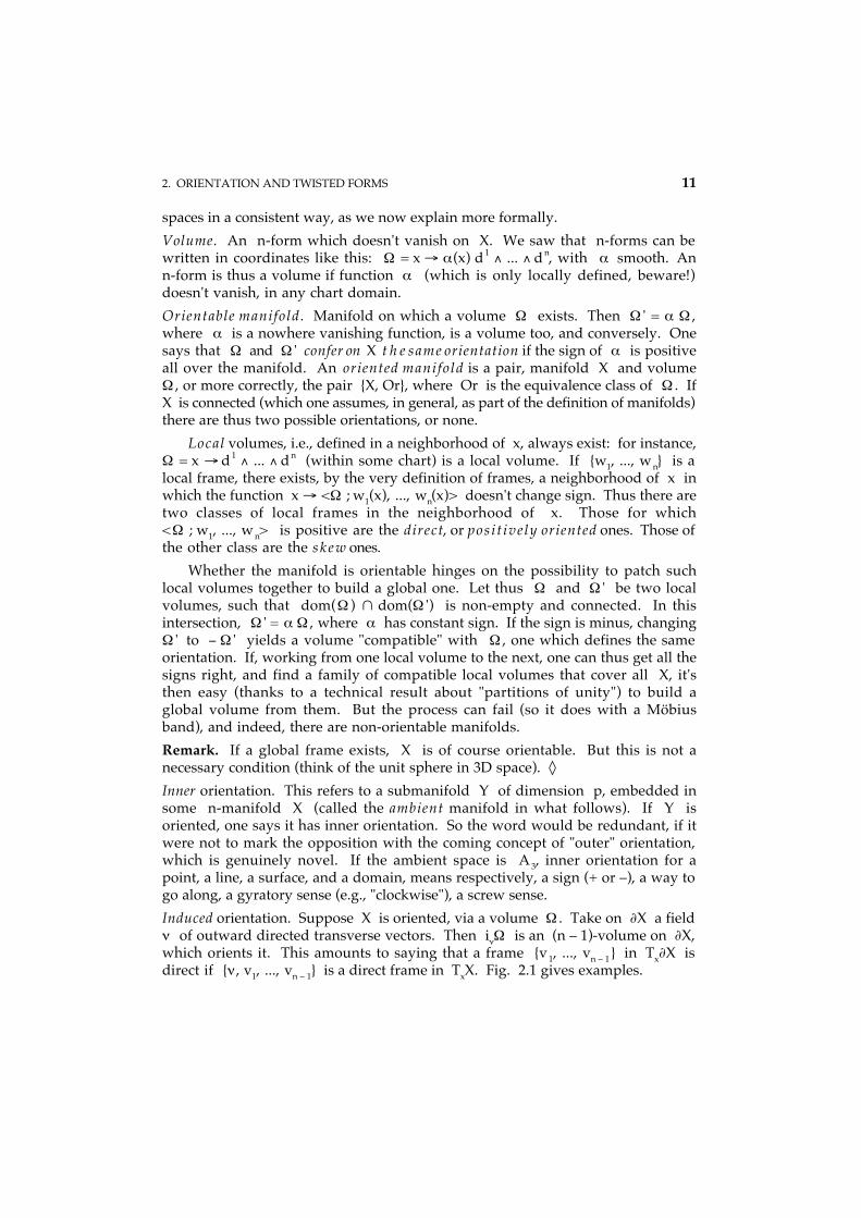
Whether the manifold is orientable hinges on the possibility to patch suchlocal volumes together to build a global one. Let thus Ω and Ω ' be two localvolumes, such that dom(Ω ) ∩ dom(Ω ') is non-empty and connected. In thisintersection, Ω ' = α Ω , where α has constant sign. If the sign is minus, changingΩ ' to − Ω ' yields a volume "compatible" with Ω , one which defines the sameorientation. If, working from one local volume to the next, one can thus get all thesigns right, and find a family of compatible local volumes that cover all X, it'sthen easy (thanks to a technical result about "partitions of unity") to build aglobal volume from them. But the process can fail (so it does with a Möbiusband), and indeed, there are non-orientable manifolds.Remark. If a global frame exists, X is of course orientable. But this is not anecessary condition (think of the unit sphere in 3D space). ◊Inner orientation. This refers to a submanifold Y of dimension p, embedded insome n-manifold X (called the ambient manifold in what follows). If Y isoriented, one says it has inner orientation. So the word would be redundant, if itwere not to mark the opposition with the coming concept of "outer" orientation,which is genuinely novel. If the ambient space is A3, inner orientation for apoint, a line, a surface, and a domain, means respectively, a sign (+ or –), a way togo along, a gyratory sense (e.g., "clockwise"), a screw sense.Induced orientation. Suppose X is oriented, via a volume Ω . Take on ∂X a fieldν of outward directed transverse vectors. Then iνΩ is an (n – 1)-volume on ∂X,which orients it. This amounts to saying that a frame v1, ..., vn – 1 in Tx∂X isdirect if ν , v1, ..., vn – 1 is a direct frame in TxX. Fig. 2.1 gives examples.


v v

ν

1

νv1

X

ν

+

–ν

ν

X

n = 1 n = 2 n = 3

2

X

v1

FIGURE 2.1. Orientation induced on ∂X by X, when the latter is, from left to right, a curve,the 2D domain between two closed curves, and the interior of a solid torus. Note, close to thelabel of each manifold, the conventional icon (± sign, arrowhead, curved arrow, helix), bywhich its inner orientation is depicted. The circles call attention upon icons that correspondto an induced orientation.

Outer orientation. A p-dimensional subspace V of a vector space U is outeroriented if a complementary subspace W (i.e., such that u = v + w, with v ∈ Vand w ∈ W, unique, for all u) has been oriented. No orientation of the ambientspace U itself is assumed. (But note that, if V is both inner and outer oriented,an orientation of U follows.) The notion extends to submanifolds (of some ambientn-dimensional manifold) the obvious way. Outer-orientation of a hypersurface,as one calls (n – 1)-submanifolds in n-dimensional ambient space, consists inproviding a crossing direction through it. If the ambient space is A3, outerorientation, for a point, a line, a surface, and a domain, means respectively, ascrew sense, a way to turn around the line, a crossing direction, a sign (+ or –).

If the ambient manifold is oriented, this provides a way to outer-orient anyorientable submanifold, and vice versa. "Outer orientability", then, is the sameas (inner) orientability. But inner and outer orientation make sense independentlyof any orientation of the ambient manifold. More, the latter need not be orientableat all. In that case, inner- and outer-orientable submanifolds do not coincide.Twisted covectors. Loosely speaking, a twisted p-covector15 at x is a pair,consisting of a covector and an orientation of TxX, it being understood that thepair formed by the opposite covector and the opposite orientation is the sametwisted covector. For those who like to see all mathematical objects as sets, thetwisted covector ω is thus the equivalence class ω, Or, −ω, − Or, composedof the two equivalent pairs just mentioned. A pair ω , Ω , where Ω is a volumeof the Or class, suffices to define ω . We shall use the notation ω ≈ ω , Ω tomean "the twisted form ω represented by the pair ω , Ω ", and abuse language

15 In contrast with other concepts in the list, it may be difficult to find good textbooks that givetwisted objects their due. Burke [Bu] does, in the wake of Veblen and Whitehead [VW] (cf. Schouten[24]). See also [Fr] and [Wr].

by saying "ω 'is' the pair ω , Ω ", etc.

2. ORIENTATION AND TWISTED FORMS 13

Twisted p-vectors. Same construction, with multivectors. Another name for twistedvector (p = 1) is a x i a l vector. (Polar vectors, thus dubbed for contrast, are justplain vectors. This dubious terminology has done and will do damage beyondreckoning [Bo].)Twisted (di f ferential) forms. Smooth fields of twisted covectors. The set of twistedp-forms over X will be denoted F p(X). Twisted n-forms are called densities.

This is a difficult concept, especially in the relatively rare16 case of non-orientable manifolds, which is also where its interest is fully revealed. If one isonly concerned with orientable ambient manifolds, a simpler definition isavailable: A twisted p-form ω is a pair ω, Or, where ω is a p-form and Ora global orientation (i.e., the class of a global volume), and ω, Or = −ω, −Orby way of definition. (Each twisted form is thus in correspondence with a pair ofordinary forms of opposite signs, and conversely. If X was not orientable, no suchcorrespondence would exist, except locally.)

Operations on twisted forms go as follows, as a rule: Take representativepairs, operate on forms, then do what it takes on orientations. For instance, if ω≈ ω , Ω, the inner product ivω is (the class of) ivω , Ω . The wedge product by astraight form η is ω ∧ η ≈ ω ∧ η , Ω. If η ≈ η, Ω ', then ω ∧ η is a straightform, equal to ± ω ∧ η , the sign being that of the ratio Ω '/Ω . See how thisprinciple applies to the next notion:Trace of a twisted p-form over ∂X. If ω is represented by ω, Ω , we know aboutthe trace tω of ω , but we need a volume on ∂X to complete the pair. For this, letn be a field of outward vectors17 on ∂X. The trace tω is then represented by thepair tω, inΩ (or by the pair − tω, − i nΩ ) .

3. INTEGRATION AND THE STOKES THEOREMLet's now review integration, where the notion of density will reveal its worth:For densities are, among all the geometrical objects living on manifolds, thosethat can be integrated.

We shall call reference p-simplex the following closed set in IRn:

(3.1) Sp = x ∈ IRp : xi ≥ 0 ∀ i ∈ [1, p], ∑ i = 1, ..., p xi ≤ 1,

and faces of Sp the subsets obtained by replacing one or more of the inequalities in(3.1) by equalities. (The empty set and the vertices thus count as faces.) A simplic ialm a p18 is a function of type Sp → Sq which is affine, one-to-one, and transformsvertices into vertices. (Each face is then transformed into another face of samedimension.) Such a map induces an injection σ from [0, p] into [0, q], obtained by

16 But not unheard of. Non-orientable manifolds do intervene in some modellings, about materialswith periodic structure, for instance, for which the "fundamental domain" of the repetitive structure,boundary points duly indentified, may form a non-orientable manifold (or worse: not be a manifold atall; see [He] for counter-examples).17 What is needed is a transverse field, but one could of course choose an inward directed one. Thechoice of an outward one agrees with current use.18 This notion, introduced here for convenience, will not serve elsewhere in this document.

calling σ(i) the number of vertex number i of Sp in the larger reference simplex.


0 1

0 1

1

S

S

S

0

1

2

X

s

s

s

s

s1

2

3

4

5

FIGURE 3.1. Examples of simplicial cells, in dimension 2.

Simplicial maps have orientation when p = q or q − 1. If p = q, the injectionσ is actually a permutation, and the map is said even or o d d according to thesignature of σ. If q = p + 1, the map is even or odd according to the signature19 ofthe permutation defined by 0, 1, ..., p + 1 → i, σ(0), σ(1), ..., σ(p), where i isthe vertex, among those of Sp + 1, which is not in the image of Sp.Simplic ia l ce l l (of dimension p). It's an embedding of Sp into X (Fig. 3.1), ormore precisely, an equivalence class (again ...) of such embeddings, the equivalencerelation being s ~ s' iff (1) the images of Sp by s and s', denoted |s| and |s'|,coincide, (2) s −1 s' is an even simplicial map. (The image |s| thus correspondsto two simplicial cells, one of each orientation.) The name "simplex" is oftenmeant to refer to the image |s|, or to s itself, by a natural abuse of language. Thediffeomorphic image of a cell is a cell.Triangulation, or simplic ial tiling of an n-dimensional differentiable manifoldX. This refers to a family S of n-dimensional simplicial cells in X, with thefollowing properties:

(a) If s and σ are two cells of S, the mapping s σ−1 is simplicial,(b) If s ≠ σ, then |s| ≠ |σ|,(c) ∪s ∈ S |s| = X,(d) Any compact part of X is contained in the set-union of a finite number of images |s|.These axioms almost correspond to the notion of mesh as used in finite element

theory, where the manifold X, of dimension 3, is the "computational domain", Dsay. (In particular, property (a) implies that the intersection of two tetrahedrais a tetrahedron, a facet, an edge, a vertex, or the empty set.) Note that theshape of the elements can be chosen at will, and be made to fit the curved boundary

19 Same notion as sign(σ, ς) above, in a slightly changed context.

of D, in particular. However, the practice of finite elements requires more than a

3. INTEGRATION AND THE STOKES THEOREM 15

mesh. One should also be able to identify nodes, edges, etc., all geometric elementsthat may eventually support a degree of freedom, hence the following refinednotion:Simplic ia l mesh of an n-dimensional differentiable manifold X. This refers to afamily S of (beware!) p-dimensional simplicial cells in X, 0 ≤ p ≤ n, withproperties (a) to (d) as above, and in addition,

(e) If |s| ∩ |σ| is not empty, there exists one and only one cell of S the image of which is |s| ∩ |σ|.

The p-cells, with p = 0, 1, 2, 3, are the nodes (or vertices), the edges, facets andtetrahedra (or volumes) of the mesh. The above "only one" restriction correspondsto common usage, but there are cases in which it should be lifted.

FIGURE 3.2 . Local refinement of a mesh. Tetrahedra near the central one, cut into 8 parts,must themselves be cut in 4, like the one on the right, or (for those like the one on the left,which shares an edge with the central one) in 2.

Note that a simplicial tiling or mesh of X induces a simplicial tiling or meshof the boundary ∂X.

A simplicial mesh S ' is finer than S if for all s ∈ S, there exists a part S" ofS ' which constitutes a simplicial mesh of |s|. (Same notion for tilings.) It's ofcourse an order relation. A given mesh can be "refined", that is, made to generatea finer one, by various subdivision procedures (Fig. 3.2 suggests one). One canmanage so that the number of cell-shapes20 generated this way stays bounded[By]. One then has uniform refinement. We'll say, rather loosely, that an orderedfamily of meshes m obtained by uniform refinement "tends to zero", denoted m →0, if the largest diameter γ m of all cells (the "grain" of the mesh) tends to 0.21

Integral of a density. Let ω = ω, Ω be a density on X, and S a simplicial tiling.Let us set

<ω ; s> = (n!)–1 <ω ; s*e1, ..., s*en> sgn[<Ω ; s*e1, ..., s*en>],

20 Shape is a metric notion, so we are a bit ahead here. Same remark about the "grain", below.21 Just "γm → 0", without the uniformity, would make sense, but wouldn't do as regards the convergenceproperties one may need in the practice of finite elements. It is well known that obtuse angles going toπ and more generally, uncontrolled "flattening" of the elements, are a bad thing [BA].


where the e is are the basis vectors in IRn (i.e., the edges 0, i of the referencesimplex). Then, set

JS (ω ) = ∑ s ∈ S <ω ; s>

(a Riemann sum). The integral of ω on X, denoted ∫X ω , is the limit, when itexists, of JS (ω ) as S runs along an ordered sequence of meshes for which γ mtends to zero.22 The sum JS (ω ) is indifferent to the orientation of the maps s,and this is why densities, and not n-forms, can be integrated.

If u is a diffeomorphism, it follows from the definition that ∫u(X) ω = ∫X u*ω .(This may be wrong, or even meaningless, otherwise.)

Twisted p-forms can be integrated on submanifolds of dimension p whenthese have outer orientation. In particular, the integral ∫∂ X ω makes sense if ωhas degree n − 1. (It's the integral of the trace, the definition of which was givenabove.) If u embeds Y, of dimension p, into X, then

∫u(Y) ω = ∫Y u*ω .

Exterior der ivat ive. If ω = x → ∑ σ ∈ C (p, n – p) ωσ(x) dσ(1) ∧ dσ(2) ∧ . . . ∧ dσ(p) is thecoordinate description of a p-form, dω is the following (p − 1)-form:

(3.2) d ω = x → ∑ σ ∈ C (p, n – p), i = 1, ..., n ∂iωσ(x) di ∧ dσ(1) ∧ dσ(2) ∧ ... ∧ dσ(p).

For a twisted form ω ≈ ω, Ω , one has dω ≈ dω, Ω , by definition. If p = 0, i.e.,if ω is a function f, df is its di f ferentia l, and <df ; v> is what was earlierdenoted (∑i v

i ∂i) f. A calculation shows that

(3.3) d(ω ∧ η) = dω ∧ η + (–1)p ω ∧ dη,

where p is the degree of ω .Exercise. Can dω ∧ ω be nonzero?Theorem (Stokes). I f ω i s a twisted (n − 1)-form, then

(3.4) ∫∂ X ω = ∫X dω .

Proof. Take a tiling of X, fine enough so that each cell be inside the domain ofsome chart. It's then easy to prove that ∫ ∂ | s | ω equals ∫ | s | dω , by working onexpression (3.2) in a chart. When all these contributions are summed up, theintegrals on inner (p − 1)-faces cancel two by two, and what remains is thecontribution of cells contained in ∂X, hence (6). ◊

Note that X need not be orientable. If it is, a corollary is available: ∫∂ X ω =∫X dω for any (n – 1)-form. [Proof: First go to ω ≈ ω , Ω , where Ω is an orientingvolume, and apply (3.4).] This, combined with (3.3), gives the integration byparts formula, for a p-form ω and a q-form η,

(3.5) ∫X dω ∧ η = (–1)p – 1 ∫X ω ∧ dη + ∫∂X ω ∧ η.

22 The dependence on the metric is only apparent, as one may work within a local chart, by usingpartitions of unity.

As another corollary, t being the foregoing trace operator,

3. INTEGRATION AND THE STOKES THEOREM 17

dt = td,

where the d on the left applies to forms living on ∂X. [Proof: For any p-form ωand any (p + 1)-manifold Y embedded in ∂X, one has ∫Y dtω = ∫∂Y tω = ∫∂Y ω =∫Y dω = ∫Y tdω .]

The interaction with pull-back, ruled by

(3.6) u*d = du*,

also stems from Stokes. [Proof: Notice that ∂(u(M)) = u(∂M) when u is anembedding. Thus ∫X du*ω = ∫∂X u*ω = ∫∂(u(X)) ω = ∫u(X) dω = ∫X du*ω , for all ω , allX, hence the result.]Chain. A p-chain over X is a formal sum c = ∑ i = 1, ..., k µi M i of orientedsubmanifolds of X all of dimension p, called here the "chain elements", with"weights" µi taken in some ring of coefficients (say IR for definiteness, thoughsuch coefficients will most often be signed integers in our examples). We distinguishstraight chains, for which all components have inner orientation and twistedchains, with outer oriented components. Chains of the same class (straight ortwisted) can be added and multiplied by a scalar, and thus form a real vectorspace. To see how, conceive c as a function, real-valued, on the set of all (inner orouter) oriented p-manifolds, with finite support (all but a finite number ofmanifolds get zero weight). Now, to add or multiply chains, add or multiplythese functions. We shall denote by Cp(X) [resp. Cp(X)] the space of straight[resp. twisted] p-chains. Integration and ∂ extend to l inear operators on thesespaces, as follows:

∂c = ∑ i = 1, ..., k µi ∂Mi, ∫c ω = ∑ i = 1, ..., k µ

i ∫Mi ω .

Remark. The concept of chain is useful in connection with the boundary operator:The boundary ∂M of an oriented submanifold M may be made of severalsubmanifolds Bi which for some reason have been provided with their ownorientations, which may agree or not with the one induced by M. Hence therepresentation of ∂M as the chain B = ∑ i β

i Bi, with βi = ± 1 according to whetherorientations agree or not. ◊

Integration provides a duality product between elements of Cp and F p [resp.of Cp and F p], which we shall emphasize by using the alternate notation< ω ; c> for ∫c ω . The Stokes theorem, <ω ; ∂c> = <dω ; c>, then makes dappear23 as the dual of ∂.L i e der ivat ive. Operation of type F p → F p, defined by Lvω = i v(dω ) + d(ivω ) ,where v is a vector field. If p = 0, then L vf = <df ; v>. When f depends on time,∂tf + Lvf is the convective der ivat ive of fluid dynamics. More on this in Section 5,where a more primitive definition, of which the present one is merely a consequence,will be given.Divergence of a vector field. Let p = n in what precedes. Then, n-forms making a

23 For dual operators, see [Yo], Chap. 7. The concept supposes a topology on Cp(X), which we havenot introduced, but this can be done (in a way which makes ∂ continuous).

one-dimensional space, Lvω = d(ivω ) is proportional to ω . The ratio div v such


that d(ivω ) = (div v) ω is called the divergence of v. Like the Lie derivative,we shall meet the divergence again later. The point of mentioning them now is tostress their non-dependence on the structural element that now comes: metric.

4. METRIC STRUCTURES ON MANIFOLDS

Metric. A smooth field of bilinear maps g ∈ Tx X × Tx X, symmetric (i.e., gx(v, w)= gx(w, v) ∀ v, w, x, and strictly posit ive definite : gx(v, v) > 0 if and only if v ≠ 0.A Riemannian manifold X, g is a manifold X provided with a metric g. Thevalues g ij = g(∂i, ∂ j) obtained for the basis vectors are called the metric coefficients.We shall abbreviate the orthogonality relation, gx(v, w) = 0, by v ⊥ w.Euclidean space. Denoted En, this is the affine space An equipped with a dotproduct of its vector associate (which provides a metric in the foregoing sense)and an orientation, which we shall denote by Or in what follows. We'll use thedot product, v · w, as an alternative to g(v, w) in the Euclidean framework, and|v| for the norm of v, defined as g(v, v)1/2.

If u ∈ [0, 1] → X is a trajectory, and if ∂tu(t) is the tangent vector at pointu(t), the integral ∫[0, 1] dt [g(∂ tu(t), ∂tu(t))]1/2 is the length of the image of u. Thelower bound of all trajectory lengths, under the condition that u(0) = x and u(1) =y, is the distance between x and y. The axioms for a distance are indeed satisfied,and providing X with a metric thus transforms it into a metric space. But it givesmore: a notion of angle, since a scalar product g x is available in each tangentspace, a notion of intrinsic curvature, etc., and a quite important structure knownas a connexion, that makes possible what was not in the general case: to comparetwo remote vectors, to know what it means for a tensor to be "constant" in theneighborhood of a point, and to measure the rates of variation of such objects,locally (notion of "covariant derivative"). For these notions and their applicationsto "gauge theories", one may refer to [Bl].Vector product of two vectors v and w. The vector v × w, orthogonal to both vand w, such that |v × w|2 + |v · w|2 = |v|2 |w|2, and such that v, w, v × wmakes a direct frame.

It's often asserted that "the vector product is an axial vector", which makesno sense (v × w is just a vector, and nothing more), unless reinterpreted in anappropriate (and different) context, as follows. The mapping v, w → v × wdepends on orientation, obviously: change Or to – Or and the vector product,according to the foregoing recipe, is now – v × w. On the other hand, the twisted(or axial) vector made of the equivalence class v × w, Or, – v × w, – Or is anorientation-independent object, well defined as soon as a metric exists. Denotingthis object by v × w, we thus define a binary operation, × , metric-dependent butindifferent to orientation, which yields an axial vector from two polar ones. If"vector product" refers to t h i s operation, then, truly, "the vector product of twovectors is an axial vector". But this implies a context, that of a non-orientedspace, which is not the one we assume.T h e isomorphism between forms and vector f i e lds . On a Riemannian manifoldX, g, let a vector field u be given, and consider the linear map v → g(u(x), v(x))

4. METRIC STRUCTURES ON MANIFOLDS 19

on Tx. This is a covector at x, that we shall denote by u(x), and the field x →u(x) is a differential form of degree 1, that we shall denote by u. Conversely, a

1-form ω generates a vector field #ω , if one defines #ω (x) as the unique vectorof Tx such that g(#ω (x), v) = < #ω (x) ; v> ∀ v ∈ Tx.

Now, take a basis, in which u = ∑i ui ∂i, and ω = ∑ i ω i d

i. Then g(u, v) =∑i, j gij u

j vi ≡ ∑i ( u)i vi, hence ( u)i = ∑i gij u

j. No harm done till there, but there isa habit to write u i instead of ( u)i and to call these numbers the "covariantcomponents" of the vector u (instead of "the components of the form u", whatthey truly are), the genuine components u i then being dubbed "contravariant".Operator is then construed as "lowering the indices", hence the symbol. Whyco and contra is not too difficult to explain (although one could make a good casefor a reversal of usage [DL]), because of what happens during a change of basis: Ifa new basis ∂' is given by ∂j = ∑ j s

ij ∂i, vector v = ∑ i v

i ∂ i becomes v = ∑i vi ∂i in the

new basis, and v i = ∑j sij v

j. So "components change in the other direction" whencompared to how basis vectors change. But there is no real parity of status between"contravariant" and "covariant" components: the former are relative to a basis,the latter are relative to a basis and t o a metric.

Conversely, of course, the components of #ω , also conventionally denoted byω i, are obtained by solving the system ∑ j g i j ω

j = ω i, i.e., by ω i = ∑ j gi j ω j, if one

denotes by g i j the entries of the inverse of the g i j matrix. This is "raising theindices". Predictably, # u = u, and #ω = ω .Remark. The norm o f a covector ω is |ω | = sup<ω ; v> : |v| = 1, by definition.It's easy to check that this norm stems from a scalar product, whose value for thepair di, dj is precisely gi j. ◊

All these subtleties evaporate, for the better or the worse, when the basis isorthonormal, i.e., |∂i| = 1 and ∂i ⊥ ∂j for i ≠ j. Then ui = ui, etc.Gradient. The gradient of a function ϕ is the vector field grad ϕ such that, usingthe above isomorphism, grad ϕ = #dϕ. Since dϕ = ∑i ∂iϕ d i, the "covariantcomponents" of grad ϕ, in the above sense, are the ∂iϕ. But its components in the ∂basis are ∑ j g

i j ∂ jϕ. Be wary that "gradient" is often used to refer to the 1-formitself rather than to its "vector representative" grad ϕ, and with good reason: dϕis well defined independently of a metric, and does its job, i.e., encoding the localrate of variation of ϕ, without it. On the other hand, change the metric and thevector representative will have to change. The latter is therefore a "proxy",metric-dependent, for "the real thing", which is the 1-form dϕ.Remark. It often happens, as here, that a vector field u corresponds, via u = #ω ,to a form ω the definition of which does not involve any metric. One may referto u, in that case, as a proxy f i e l d. One should not jump to the conclusion that allvector fields of physics are proxies of this kind. The one that describes the instantvelocity of a fluid mass, for instance, is genuinely a vector field. (Recall the verydefinition of a tangent vector as a velocity.) ◊

From now on (and hopefully, no confusion with the dimension of X shouldoccur), n denotes the "outward going normal vector field", a vector field, whosedomain contains ∂X, such that |n| = 1 and n(x) ⊥ v ∀ v ∈ Tx at all boundarypoints. The normal part nω of a form ω of degree p ≥ 1 is t i nω . Note that n u =

Thenormal partnω ofaform ω ofdegree p≥1 is tinω


g(n, u) ≡ n · u , i.e., the normal component of u.Hodge operator. Denoted ∗, and defined as follows. Let ω x be a p-covector at xand Ω a local volume. Let v1, ..., vn be a direct frame which is orthonormal (inthe sense of g), and ηx the unique (n − p)-covector such that

(4.1) ηxvp + 1, ..., vn = ω x(v1, ..., vp .

One denotes by ∗ω the twisted form x → ηx, Ω. If ω ≈ ω, Ω , ∗ω is theordinary form x → ηx. Observe that ∗∗ = ± 1, depending on the parities of n andp. More precisely, ∗∗ = (– 1)(n – 1)p, where p is the degree of the operand.

In dimension 2, where the Hodge of a 1-form is a 1-form (a twisted one), therelation between proxies has some interest. The vector #∗ u derives from u by"90° rotation" in the tangent plane. This of course refers to the metric (via thenotion of orthogonality) but to the orientation as well: Orientation is what tellsus which way to "rotate". Observe that #∗ u is a twisted vector field, if u waspolar, and the other way round.

Worth mentioning also is this:

(4.2) ∗n = t∗,

where ∗ on the left is the Hodge operator on ∂X. [Proof: Take an orthonormalbasis n, v 2, ..., vn, with all v i's tangent to ∂X. Then <∗nω ; vp + 1, ..., vn> =<nω ; v2, ..., vp> = <ω ; n, v2, ..., vp> = <∗ω ; vp + 1 , ..., vn>.] As a corollary, ∗t =(–1)p n∗, where p is the degree of the form to which this is applied.Curl. The compact definition is rot u = #∗d u. Only in three dimensions does thismake sense: Start from a vector field u, take the d of the corresponding 1-form,hence a 2-form the Hodge dual of which is a twisted 1-form. The latter has aproxy field, which is the curl of u, here denoted rot u.

Note that rot u depends on orientation, since ∗ does. Changing Or to – Orchanges it to – rot u. Just as with the vector product, one may define an axialvector field, the equivalence class rot u, Or, –rot u, – Or, represented by rot uor – rot u depending on which orientation is selected. This object only depends onthe metric structure. Hence the frequent casual (and possibly confusing) remarkthat "rot u is actually an axial vector field". In the same spirit, one can definethe curl of an axial vector field, which is then polar. Let's stress again that wed o assume an orientation here, hence a context in which axial and polar vectorsdo not fit.

One may define the curl in dimension two, by the same process, but the result∗d u is a (twisted) scalar field. There is some sense also in introducing the notation"rot ϕ", where ϕ is a function, for the vector – ⊥ grad ϕ, i.e., grad ϕ rotated 90°clockwise. We'll do that in a moment.

In 3D Euclidean space, there is a notation which may help see what's goingon. Recall that g(v, w) is now v · w , at all points, and that an orientation isselected, which gives sense to the cross product v × w. We'll take the 3-formvol(u, v, w) = u · v × w as representative24 of the direct orientation class, calledOr. Now let's proceed.


Start from a vector field u. At point x, the map v → u(x) · v is a covector.The field these covectors make is a 1-form, that we shall denote by 1u. But fromthe same vector field, one may also build a 2-form 2u, from the 2-covectors v, w→ u(x) · (v × w). So u can act as proxy for two different forms, 1u and 2u.Similarly, a scalar field ϕ generates a 0-form 0ϕ, which is just ϕ itself, and a3-form 3ϕ, defined as the field of 3-covectors u, v, w → u · (v × w) ϕ(x), i.e., ϕtimes the standard volume. Conversely, by the Riesz representation theorem,p-covectors in dimension 3 must be of one of these four kinds, and hence, a form in3D must be 0ϕ, 1u, 2u, or 3ϕ, depending on its degree, for some scalar or vector proxyϕ or u. (Notice how both metric and orientation play a role in the correspondence.)The notation 1u is of course redundant with u, but is clearer in the Euclidean 3Dcontext.

Now, it's easy to show that

(4.3) 1(grad ϕ) = d 0ϕ, 2(rot u) = d 1u, 3(div u) = d 2u

and to see what the integral of a form means: The integral of 0ϕ at point x is just± ϕ(x), the sign being the orientation of the point (see above). The integral ∫c

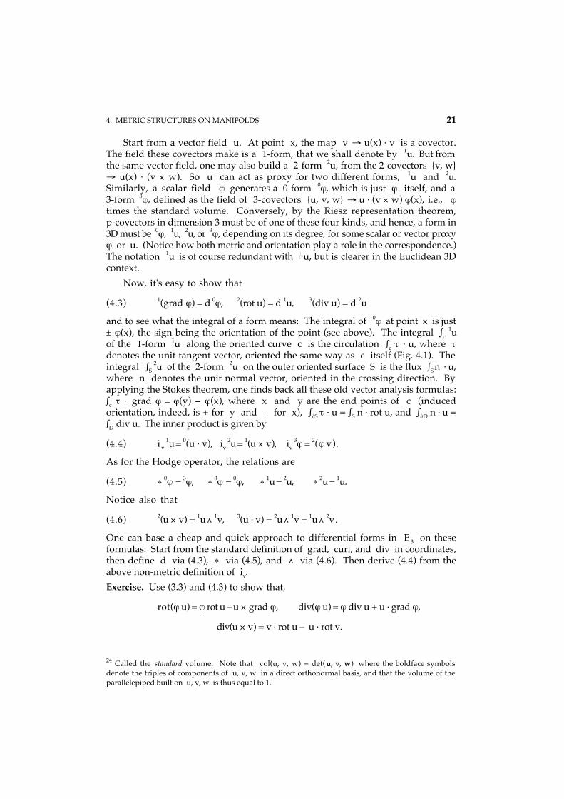
1uof the 1-form 1u along the oriented curve c is the circulation ∫c τ · u, where τdenotes the unit tangent vector, oriented the same way as c itself (Fig. 4.1). Theintegral ∫S

2u of the 2-form 2u on the outer oriented surface S is the flux ∫S n · u,where n denotes the unit normal vector, oriented in the crossing direction. Byapplying the Stokes theorem, one finds back all these old vector analysis formulas:∫c τ · grad ϕ = ϕ(y) – ϕ(x), where x and y are the end points of c (inducedorientation, indeed, is + for y and – for x), ∫∂S τ · u = ∫S n · rot u, and ∫∂D n · u =∫D div u. The inner product is given by

(4.4) i v 1u = 0(u · v), iv

2u = 1(u × v), iv 3ϕ = 2(ϕ v).

As for the Hodge operator, the relations are

(4.5) ∗ 0ϕ = 3ϕ, ∗ 3ϕ = 0ϕ, ∗ 1u = 2u, ∗ 2u = 1u.

Notice also that

(4.6) 2(u × v) = 1u ∧ 1v, 3(u · v) = 2u ∧ 1v = 1u ∧ 2v.

One can base a cheap and quick approach to differential forms in E3 on theseformulas: Start from the standard definition of grad, curl, and div in coordinates,then define d via (4.3), ∗ via (4.5), and ∧ via (4.6). Then derive (4.4) from theabove non-metric definition of iv.Exercise. Use (3.3) and (4.3) to show that,

rot(ϕ u) = ϕ rot u – u × grad ϕ, div(ϕ u) = ϕ div u + u · grad ϕ,

div(u × v) = v · rot u – u · rot v.

24 Called the standard volume. Note that vol(u, v, w) = det(u, v, w) where the boldface symbolsdenote the triples of components of u, v, w in a direct orthonormal basis, and that the volume of theparallelepiped built on u, v, w is thus equal to 1.


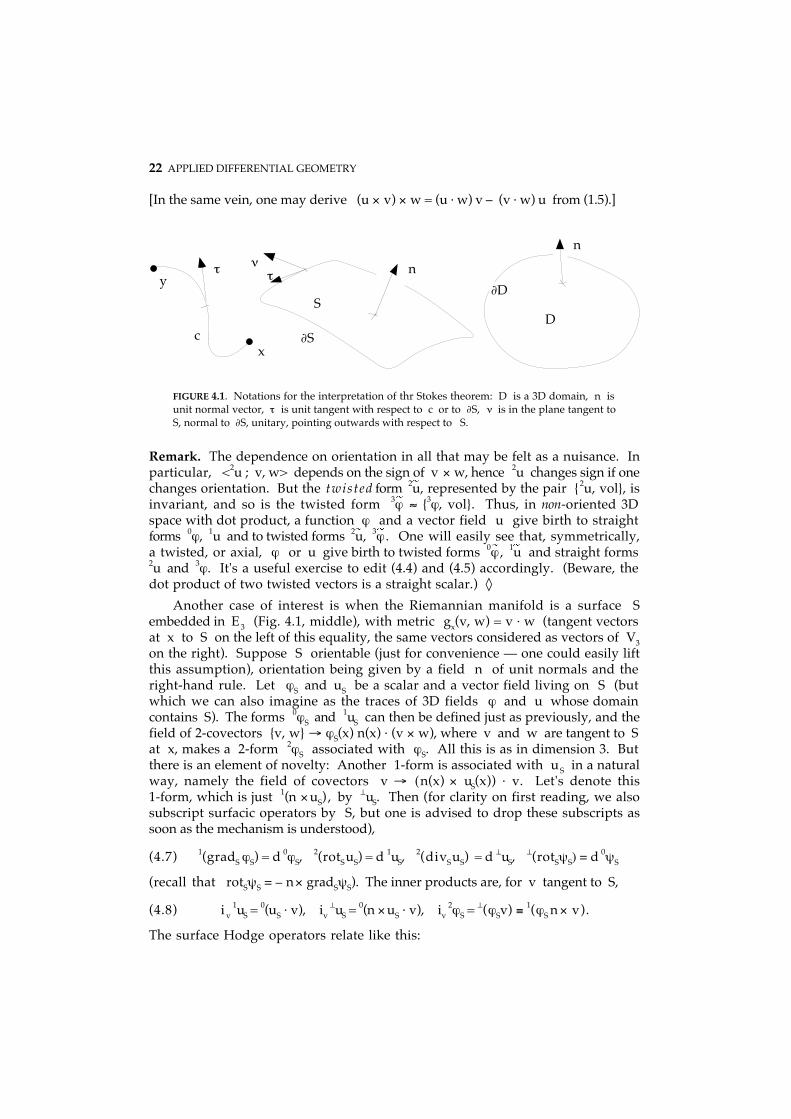
[In the same vein, one may derive (u × v) × w = (u · w) v – (v · w) u from (1.5).]

D

∂D

n

nτ

S

∂S

ν

c

τ

x

y

FIGURE 4.1. Notations for the interpretation of thr Stokes theorem: D is a 3D domain, n isunit normal vector, τ is unit tangent with respect to c or to ∂S, ν is in the plane tangent toS, normal to ∂S, unitary, pointing outwards with respect to S.

Remark. The dependence on orientation in all that may be felt as a nuisance. Inparticular, <2u ; v, w> depends on the sign of v × w, hence 2u changes sign if onechanges orientation. But the twisted form 2u, represented by the pair 2u, vol, isinvariant, and so is the twisted form 3ϕ ≈ 3ϕ, vol. Thus, in non-oriented 3Dspace with dot product, a function ϕ and a vector field u give birth to straightforms 0ϕ, 1u and to twisted forms 2u, 3ϕ . One will easily see that, symmetrically,a twisted, or axial, ϕ or u give birth to twisted forms 0ϕ , 1u and straight forms2u and 3ϕ. It's a useful exercise to edit (4.4) and (4.5) accordingly. (Beware, thedot product of two twisted vectors is a straight scalar.) ◊

Another case of interest is when the Riemannian manifold is a surface Sembedded in E3 (Fig. 4.1, middle), with metric gx(v, w) = v · w (tangent vectorsat x to S on the left of this equality, the same vectors considered as vectors of V3on the right). Suppose S orientable (just for convenience — one could easily liftthis assumption), orientation being given by a field n of unit normals and theright-hand rule. Let ϕS and uS be a scalar and a vector field living on S (butwhich we can also imagine as the traces of 3D fields ϕ and u whose domaincontains S). The forms 0ϕS and 1uS can then be defined just as previously, and thefield of 2-covectors v, w → ϕS(x) n(x) · (v × w), where v and w are tangent to Sat x, makes a 2-form 2ϕS associated with ϕS. All this is as in dimension 3. Butthere is an element of novelty: Another 1-form is associated with uS in a naturalway, namely the field of covectors v → (n(x) × uS(x)) · v. Let's denote this1-form, which is just 1(n × uS) , by ⊥uS. Then (for clarity on first reading, we alsosubscript surfacic operators by S, but one is advised to drop these subscripts assoon as the mechanism is understood),

(4.7) 1(gradS ϕS) = d 0ϕS, 2(rotS uS) = d 1uS,

2(divS uS) = d ⊥uS, ⊥(rotSψS) = d 0ψS

(recall that rotSψS = – n × gradSψS). The inner products are, for v tangent to S,

(4.8) i v 1uS = 0(uS · v), iv

⊥uS = 0(n × uS · v), iv 2ϕS = ⊥(ϕSv) ≡ 1(ϕS n × v).

The surface Hodge operators relate like this:


(4.9) ∗S 0ϕS = 2ϕS, ∗S

2ψS = 0ψS, ∗S 1uS = ⊥uS, ∗S

⊥uS = – 1uS.

Remark. The normal part of 1u is 0(n · u), the normal part of 2u is – 1(n × u), thatis to say, – ⊥uS. On the other hand, tS

1u = 1uS, tS 2 u = 2(n · u). This checks with

(4.2), i.e., ∗S nS = tS ∗S, as it should. Also, n · rot u = rotS uS, a case of td = dt. ◊Scalar product of two p-forms. If ω and ω ' ∈ F p, the exterior product ω ∧ ∗ω' isa density, so ∫X ω ∧ ∗ω ' makes sense. This quantity is defined as the scalarproduct of ω and ω ' , here denoted (ω , ω '). Symmetry and positivity stem from(1.2) and (4.1). Remark also that (∗ω, ∗ω') = (ω , ω '). The norm of ω is thendefined as (ω , ω )1/2, equal to [∫X ω ∧ ∗ω]1/2. All this turns F p into a pre-Hilbertianspace. By completion, one gets a Hilbert space of forms, denoted Fp, which is top-forms what space L2

was to functions.The adjoint of d, with respect to this scalar product, is called the codifferential,

denoted δ. Thanks to (3.5) and (4.2), the domain of δ is ω ' ∈ F p + 1 : nω ' = 0and δ = (–1)np + 1 ∗d∗. [Proof: p being the degree of ω , one has (dω , ω ') = ∫ dω ∧∗ω' = (–1)p + 1 ∫ ω ∧ d∗ω' = (–1)p + 1 + p(n – p) ∫ ω ∧ ∗∗d∗ω' = (ω , δω' ), since p2 = p mod2.] But be careful: Here, p is not the degree of ω ', to which δ is to be applied.The usable formula, where q is the degree of the form to which both sides mustapply, is δ = (–1)n(q – 1)+ 1 ∗d∗. (We had p = q – 1 in the proof.) These minus signsare an unavoidable nuisance. Fortunately, there is not much use for δ, apart fromits role in the definition of the Laplacian operator on forms: This is δd + dδ, up toan optional minus sign. Hence the well known formulas ∆ = div grad and – ∆ =rot rot – grad div, when applied to a scalar or a vector proxy.

Let's use L2 for the space of square summable fields, be they scalar or vectorvalued. The functional spaces

L2grad = ϕ ∈ L2 : grad ϕ ∈ L2, L2

rot = u ∈ L2 : rot u ∈ L2, L2div = u ∈ L2 : div u ∈ L2 ,

with their natural scalar products, such as ((ϕ, ϕ')) = ∫X ϕ ϕ' + ∫X grad ϕ · grad ϕ' ,etc., correspond (for p = 0, 1, 2) to the Hilbert space Fp

d obtained by completion ofF p with respect to the norm induced by the scalar product ((ω , η)) = ∫X ω ∧ ∗η +∫X dω ∧ ∗dη. When X is the 3D domain of Fig. 4.1, the classical integration byparts formulas,

(4.10) ∫D v · grad ϕ = – ∫D ϕ div v + ∫∂D n · v ϕ,

(4.11) ∫D u · rot v = ∫D v · rot u – ∫∂D n × u · v,

appear as particular cases of a single formula, namely (3.5). In two dimensions,e.g., when X is the surface S of Fig. 4.1, (3.5) yields the 2D version of (4.10), i.e.,

(4.12) ∫S vS · gradS ϕS = – ∫S ϕS divS vS + ∫∂D ν · vS ϕS,

and

(4.13) ∫S uS · rotS ϕS = ∫S ϕS rotS uS – ∫∂S n · (ν × uS) ϕS

which is nothing else than (4.12) with vS = n × uS, since divS(n × uS) = – rotS uS.(What about dropping all these S's, by the way?)


5. THE LIE DERIVATIVEIn Electromagnetism (our main intended domain of application), differential formsmodel "fields", in the physical sense of the word. Such fields are probed, measured,with help of devices that are mathematically represented by manifolds, andintegrals are the results of such experiments. The case of the electric field (a1-form, denoted e), measured by a voltmeter, which displays the electromotiveforce (emf) along the conductive thread (a 1-dimensional, inner oriented manifoldc), is typical: The emf is ∫c e. As a rule, the rates of variation, as time goes on, ofsuch integral quantities, are physically meaningful. Typical again in this respectis Faraday's law, whose mathematical expression is dt ∫S b + ∫∂S e = 0 for allinner-oriented surfaces S, with b a 2-form, called magnetic induction.

Observers in relative motion, then, get different views of the field, becausethe rate of variation of what they measure with any given probe will depend onhow the latter is moving. The Lie derivative is the mathematical tool by whichsuch rates of variation are handled.

Motion is conveniently described by a smoothly time-dependent family u ofdiffeomorphisms ut : X → X. (One may always assume that u0(x) = x. We shallallow ourselves to omit the t, or on the contrary to use the developed notationu(t, x) , as most convenient.) For each x, there is a trajectory t → ut(x), or orbit,whose tangent vectors v t(y) ≡ v(t, y) = ∂tu(t, u t

–1(y)) make the velocity field attime t. One may imagine X as filled up with a fluid and construe u t(x) as thetrajectory of the particle that passes at x at time 0, and v as its velocity,although of course no such interpretation is compulsory. The trajectories are integralcurves of the field v, in the sense that t → u(t, x) solves the differential equationdtg = v(t, g(t)) with initial condition g(0) = x.

Of particular interest is the case when the family of maps ut satisfies

(5.1) ut + s (x) = us(ut(x))

for all x, s, and t, thus forming a one-parameter group of diffeomorphisms . Thenv is time-independent25 [proof: v(t, x) dt ~ ut + dt (ut

–1(x)) – ut(ut–1(x)) = udt(x) – x ~

v(0, x) dt], and u is called its f l o w. Notice that v is invariant under push-forwardsof its own flow. [Proof: (ut)*(x) v(x) dt ~ ut(udt(x)) – ut(x) = udt(ut(x)) – ut(x) ~v(ut(x)) dt.]Homotopy. This is the mathematization of the concept of "morphing", i.e.,"continuous deformation", as made familiar by many movies. Two continuous mapsf and g from a topological space X to a topological space Y are homotopic ifthere exists a continuous map u from [0, 1] × X (endowed with the producttopology) to Y such that f = x → u(0, x) and g = x → u(1, x). [Imagine X as anobject, f as its graphical representation on, say, a computer screen, here modelledby Y. Then x → u(t, x) is an image which deforms with t, passing continuouslyfrom f to g.] If X = Y and f is the identity, one says that g is a deformation of

25 Conversely, a smooth vector field generates a flow, if one is content with local existence (in spaceand time).

X. If, moreover, g maps X to one of its points, the homotopy is a contraction.

5. THE LIE DERIVATIVE 25

Space X is then said to be contractible. Examples: Affine spaces are contractible.A ball is contractible, a sphere is not. Flow, we see, is an instance of homotopy.Extrusion of a manifold. Suppose v is transverse to a submanifold M (whichmust therefore have dimension p < n). The union ext(ut, M) of the images u s(M)for 0 ≤ s ≤ t makes an embedded (p + 1)-manifold, for t small enough,26 calledthe extrusion of M over the lapse of time [0, t].

u (S)t

Sext(u , S)t

ext(u , ∂S)tS

∂S

v v

v

v v

∂S

u (∂S)t

FIGURE 5.1 . Extrusion of a surface S by the flow of a vector field v, and the interplay oforientations.

If M is oriented, this orients the extrusion, as follows: If v1, ..., vp is adirect frame at x ∈ M, consider v(x), v1, ..., vp (which i s a frame, by transversalityof v) as direct. We note that, with this convention, the boundary of the extrusionis the p-chain

(5.2) ∂[ext(ut, M)] = ut(M) – M – ext(ut, ∂M)

and ∂[ext(ut, ∂M)] = ut(∂M) – ∂M. (Cf. Fig. 5.1, where M is the surface denoted S.)Proposition 5.1. The integral of a (p + 1)-form η over ext(ut, M) i s

∫0t dτ ∫uτ (M) i vη.

Proof. Take a simplicial tiling S of M, and split the interval [0, t] into segments[kδt, (k + 1)δt], k = 0, ..., N, with (N + 1)δt = t. Extrude each simplex s of S andsplit the extrusion into slices of the form ext[u((k + 1)δt), s] – ext[u(k δt), s]. Eachslice can then be cut into simplices (three, if p = 2; how many in general?). FormRiemann sums and go to the limit. ◊

When u is a flow, this simplifies a bit:

(5.3) <η ; ext(ut, M)> = t <ivη ; M>,

because all integrals over uτ(M) are equal, owing to the invariance of v.Now the Lie derivative of a p-form ω with respect to the flow of a vector

field v is defined, at time t = 0, by

26 If ϕ : S → IRp is a chart for S, s, x → s, ϕ(x) ∈ IRp + 1 makes one for the extrusion, providedpoints u s(x) for s ∈ [0, t] are all distinct. In case v depends on time, transversality is understood asholding at time 0. Smoothness in time of v, anyway, warrants it for s small enough.

(5.4) Lvω = lim t → 0 1/t [ut*ω – ω ].


(The concept makes sense for all kinds of tensors, actually. In particular, the Liederivative Lvw of a vector field w is the Lie bracket [v, w].) Intuitively, Lvω isthe rate of variation of ω "as transported by" the flow of v, and "as measured bya fixed observer" (the "fisherman's derivative" of Arnold [Ar]). To express Lv interms of already known entities, let's consider the integral ∫M ut*ω , with a fixedM. After (5.2),

∫M ut*ω – ∫M ω = ∫ut(M) ω – ∫M ω = <ω ; ∂[ext(ut, M)]> + <ω ; ext(ut, ∂M)>

= <dω ; ext(ut, M)> + <ω ; ext(ut, ∂M) >.Using (5.3) twice (once with η = dω , then again but on ∂M and with η = ω ), wefind ∫M Lvω = <ivdω ; M> + <ivω ; ∂M>. Using Stokes, we may conclude:Proposition 5.2. Lv = ivd + div.Consequently, Lvu* = u*Lu*v

, after (1.4) and (3.6), and Lvu* = u*Lv if v is stationary.I f ω is time-dependent, we see that

(5.5) dt[∫ut(M) ω ] t = 0 = ∫M [∂tω + Lvω ],

which prompts us to define the convective derivative ∂ tω + Lvω of ω withrespect to the flow. (That v may depend on time is not a concern here; what isconsidered is the flow of v as frozen at its value at time 0).) It may be useful alsoto have the derivative at time t, which is given by the formula

(5.6) ∂t(ut*ω ) = ut*(∂tω + Lvω ) .

Another way to express that, thanks to Leibniz's rule, is

(5.7) ∂tut* = ut* Lv(t) = Lv(0) ut* .

All these formulas have useful applications, in different contexts.Exercise. Show that ivLv = Lvi v, that dLv = Lvd.

Before giving a few examples, let's work out Lv in 3D Euclidean space. Thanksto (4.3) and (4.4), one has:

(5.8) Lv 0ϕ = 0(v · grad ϕ) ,

(5.9) Lv 1u = 1(– v × rot u + grad(v · u)),

(5.10) Lv 2u = 2(v div u – rot(v × u)),

(5.11) Lv 3ϕ = 3(div(ϕ v)) ≡ 3(v · grad ϕ + ϕ div v).

While we are at it, the analogous formulas on a surface (all right, no S subscripts)are (5.8), unchanged,

(5.12) Lv 1u = ⊥(v rot u) + 1(grad(v · u)) ≡ 1(n × v rot u + grad(v · u)),

(5.13) Lv ⊥u = ⊥(v div u) – 1(grad(v × u)) ≡ ⊥(v div u – rot(v × u)),

not so different from (5.9) and (5.10), and


(5.14) Lv 2ϕ = 2(div(ϕ v)),

the same as (5.11).Physics provides familiar examples. For instance, if ϕ is the temperature of

a fluid mass, the rate of variation of the temperature of a material particle, asobserved at point x and time t as the particle flies by, is ∂tϕ + v · ∇ϕ, which isconsistent with (5.8). If the fluid has density q, conservation of its mass is expressedby ∂ t

3q + Lv 3q = 0, that is ∂ tq + div(q v) = 0, as can be read off from (5.11). And

(5.10) explains why the effective electric field in a moving conductor (the field towhich the current density is proportional) is e + v × b, where e and b (divergence-free) are the laboratory-frame electric field and magnetic induction. For indeed,d(e + v × b) = de – Lvb, and ∂tb + Lvb + d(e + v × b) = 0 expresses Faraday's law inthe comoving frame.Lie and wedge. Contrary to the d, the Lie derivative behaves like a genuinederivation, i.e., it respects Leibniz's rule:

(5.15) Lv(ω ∧ η) = Lvω ∧ η + ω ∧ Lvη.

Proof. Since u*(ω ∧ η ) = u*ω ∧ u*η, one has u*(ω ∧ η ) – ω ∧ η = u*ω ∧ u*η –ω ∧ η = (ω + u*ω – ω ) ∧ (η + u*η – η) – ω ∧ η = (u*ω – ω ) ∧ η + ω ∧ (u*η – η) +(u*ω – ω ) ∧ (u*η – η). Now take u = ut, divide by t, and let t go to 0. The resultstems from (5.4). ◊

Proposition 2 suggests another proof, which avoids the passage to the limit,but is more delicate. By (1.5) and (3.3), one has, with p = degree(ω ) ,

i vd(ω ∧ η) = iv(dω ∧ η + (–1)p ω ∧ dη) )

= ivdω ∧ η – (–1)p dω ∧ i vη + (–1)p ivω ∧ dη + ω ∧ i vdη

and

div(ω ∧ η) = d(ivω ∧ η + (–1)p ω ∧ i vη)

= divω ∧ η – (–1)p i vω ∧ dη + (–1)p dω ∧ i vη + ω ∧ divη,

and extra terms cancel nicely.The Poincaré Lemma. In A n, and in more general conditions as we shall see in amoment, dω = 0 implies the existence of a (p – 1)-form α such that ω = dα. Thisis a particular case of the following representation formula, derived from (5.6):

u1*ω = u0*ω + ∫01 ut* Lvω dt,

provided the u ts are defined over the semi-open interval [0, 1[. If things can bearranged so that u is a contraction u1

* is the identity and u0* = 0, so ω =∫0

1 ut* Lvω dt, that is to say, thanks to the commutation relations u*Lv = Lvu*,

(5.16) ω = d[∫01 ivut*ω dt] + iv[∫0

1 ut* dω dt] = dα + β,

If dω = 0, then β = 0, hence the Lemma: ω = dα, which we see is valid for allcontractible manifolds.


For instance, o being an arbitrary origin in En, set ut(x) = o + t(x – o), which isthe flow of the vector field x → x – o, which from now on we denote by x. This isa contraction. We note that (u t)* w = ut(x + w) – ut(x) = tw, so (ut)* is the homothetictransformation w → tw. Hence (ut*ω )(x) = tp ω (tx)) if ω has degree p, and

α(x) = ∫01 tp – 1 i xω (tx) dt, β(x) = ∫0

1 tp i xdω (tx) dt,

If ω = 1e, with rot e = 0, we thus find that u = grad ψ with

ψ(x) = x · ∫01 e(tx) dt,

a not so obvious fact. Even less obvious, if ω = 2b with div b = 0, then u = rot awith

(5.17) a(x) = – x × ∫01 t b(tx) dt,

and any scalar field q (since, automatically, d 3q = 0) is of the form q = div d,with

d(x) = x ∫01 t2 q(tx) dt.

If dω = 0, then β = 0, hence the Lemma: ω = dα. With the present choice of u t,one has more, by working out (5.16).

Let us note (with [Ko] and [Sk]) that x · a(x) = 0 in (5.17): this constraint,which selects one of the vector potentials a such that rot a = b, differs from themore common "gauges" of Coulomb and Lorenz.27 It is called Poincaré's gauge [Br,Cr], and axial gauge by some.

REFERENCES

Classic treatises are [16, 22]. Among others, which all treat the subject in some interestingway, I would more particularly recommend [4, Bu, Fk, 20, 24, 25].

[2] R. Abraham, J.E. Marsden: Foundations of Mechanics, The Benjamin/CummingsPublishing Company, Inc. (Reading, Mass.), 1978.

[3] R. Abraham, J.E. Marsden, T. Ratiu: Manifolds, Tensor Analysis, and Applications,Addison-Wesley (London), 1983.

[Ap] F. Apéry: Models of the Real Projective Plane, Vieweg (Braunschweig), 1987.[Ar] M.A. Armstrong: Basic Topology, McGraw-Hill (London), 1979.[4] V. Arnold: Méthodes mathématiques de la physique classique, Mir (Moscou),

1976.[BA] I. Babus˙ka, A.K. Aziz: "On the angle condition in the finite element method", SIAM. J.

Numer. Anal., 13, 2 (1976), pp. 214-26.[5] J. Barbotte: Le calcul tensoriel, Bordas (Paris), 1948.[B&] M. Barnabei, A. Brini, G.-C. Rota: "On the Exterior Calculus of Invariant Theory", J.

Algebra, 96 (1985), pp. 120-60.

27 No t in the name of this Lorenz. who is the Dane L. Lorenz (the same one who introducedretarded potentials [Lo]), not the Dutch H.A. Lorentz of Relativity and Lorentz force. Cf. [Bl], whorefers to Whittaker'sHistory of the Theories of Aether and Electricity, vol. 1 p. 268 [Wt], on this point ofhistory. The same source is quoted by [NC], who write "Lorentz gauge" notwithstanding.

[Be] M.V. Berry: "Anticipations of the geometric phase", Physics Today, 43, 12 (1990), pp.


34-40.[By] J. Bey: "Tetrahedral Grid Refinement", Computing, 55, 4 (1995), pp. 355-78.[Bl] J. Van Bladel: "Lorenz or Lorentz?", IEEE Antennas and Propagation Magazine,

33, 2 (1991), p. 69.[Bl] D. Bleeker: Gauge Theory and Variational Principles , Addison-Wesley (Reading,

Mass.), 1981.[Bo] A. Bossavit: "On axial and polar vectors", ICS Newsletter, 6, 3 (1999), pp. 12-14.[Br] U. Brehm: "How to Build Minimal Polyhedral Models of the Boy Surface", Math. Intell.,

12, 4 (1990), pp. 51-56.[Br] W.E. Brittin, W.R. Smythe, W. Wyss: "Poincaré gauge in electrodynamics", Am. J. Phys.,

50, 8 (1982), pp. 693-6.[7] W.L. Burke: Spacetime, Geometry, Cosmology, University Science Books (Mill

Valley, CA 94941), 1980.[Bu] W.L. Burke: Applied Differential Geometry , Cambridge University Press (Cambridge,

U.K.), 1985.[Ca] É. Cartan: "La théorie des groupes et la géométrie", L'Enseignement Mathématique,

26 (1927), pp. 200-25.[9] H. Cartan: Formes différentielles, Hermann (Paris), 1967.[10] Y. Choquet-Bruhat: Géométrie différentielle et systèmes extérieurs, Dunod (Paris),

1968.[Cr] F.H.J. Cornish: "The Poincaré and related gauges in electromagnetic theory", Am. J.

Phys., 52, 5 (1984), pp. 460-2.[Co] H.S.M. Coxeter: The Real Projective Plane, Springer-Verlag (New York), 1993.[11] M. Crampin, F.A.E. Pirani: Applicable Differential Geometry, Cambridge U.P.

(Cambridge), 1986.[DL] R.P. DeLong: "Change Terminology at the Turn of the Century", Notices AMS, 46, 7

(1999), p. 766.[DP] C.T.J. Dodson, P.E. Parker: A User's Guide to Algebraic Topology, Kluwer (Dordrecht),

1997.[13] B. Doubrovine, S. Novikov, A. Fomenko: Géométrie contemporaine, méthodes et

applications (2e partie), Mir (Moscou), 1982.[14] D.G.B. Edelen: Applied Exterior Calculus, Wiley (New York), 1985.[Fr] G.K. Francis: A Topological Picturebook, Springer-Verlag (New York), 1987.[Fk] Th. Frankel: The Geometry of Physics, An Introduction, Cambridge U.P. (Cambridge),

1997.[Fu] W. Fulton: Algebraic Topology, A First Course, Springer-Verlag (New York), 1995.[15] M. Göckeler, T. Schücker: Differential Geometry, Gauge Theories, and Gravity,

Cambridge U.P. (Cambridge), 1987.[He] A. Henle: A Combinatorial Introduction to Topology, Dover (New York), 1994.

(First pub., Freeman (San Francisco), 1979.)[Hs] D. Hestenes: "Vectors, Spinors, and Complex Numbers in Classical and Quantum Physics",

Am. J. Phys., 39, 9 (1971), pp. 1013-27.[HW]P.J. Hilton, S. Wylie: Homology Theory, An Introduction to Algebraic Topology,

Cambridge U.P. (Cambridge), 1965.[HP] P. Hilton, D. Holton, J. Pedersen: Mathematical Vistas, From a Room With Many

Windows, Springer (New York), 2002.[EDM] S. Iyanaga, Y. Kawada (eds.): Encyclopedic Dictionary of Mathematics , The MIT

Press (Cambridge, Ma.), 1980.[Jä] K. Jänich: Vector Analysis, Springer (New York), 2001.[16] S. Kobayashi, K. Nomizu: Foundations of Differential Geometry (2 Vols.), J. Wiley

& Sons (New York), 1963.


[Ko] D.H. Kobe: "Poincaré gauge is the multipolar gauge", Am. J. Phys., 51, 2 (1983), p. 105.[La] I. Lakatos: Proofs and Refutations, The Logic of Mathematical Discovery, Cambridge

U.P. (Cambridge), 1976.[Lo] L. Lorenz: "On the identity of the vibrations of light with electrical currents", Philos.

Mag., 34 (1867), pp. 287-301.[MT] I. Madsen, J. Tornehave: From Calculus to Cohomology: de Rham cohomology

and characteristic classes, Cambridge University Press (Cambridge), 1997.[18] P. Malliavin: Géométrie différentielle intrinsèque, Hermann (Paris), 1972.[19] J.E. Marsden, T.J.R. Hughes: Mathematical Foundations of Elasticity , Prentice-Hall

(Englewood Cliffs, N.J.), 1983.[Ma] W.S. Massey: A Basic Course in Algebraic Topology, Springer-Verlag (New York),

1991.[Mi] J.W. Milnor: Topology from the differentiable viewpoint, The University Press of

Virginia (Charlottesville), 1965.[20] C.W. Misner, K.S. Thorne, J.A. Wheeler: Gravitation, Freeman (New York), 1973.[NC] R.D. Nevels, K.J. Crowell: “A Coulomb gauge analysis of a wire scatterer”, IEE Proc.-H,

137, 6 (1990), pp. 384-8.['N] B. O'Neill: Semi-Riemannian Geometry With Applications to Relativity, Academic

Press, Boston (1983).[21] S. Parrott: Relativistic Electrodynamics and Differential Geometry, Springer-Verlag

(New York), 1987.[Pe] P. Petersen: "Aspects of global Riemannian geometry", Bull. AMS, 36, 3 (1999), pp.

297-344.[22] G. de Rham: Variétés différentiables, Hermann (Paris), 1960.[RF] V. Rohlin, D. Fuchs: Premier cours de topologie, Mir (Moscou), 1981.[24] J.A. Schouten: Tensor analysis for physicists, Dover (New York), 1989.[25] B. Schutz: Geometrical methods of mathematical physics , Cambridge University

Press (Cambridge, U.K.), 1980.[ST] I.M. Singer, J.A. Thorpe: Lecture Notes on Elementary Topology and Geometry ,

Springer-Verlag (New York), 1967.[Sk] B.-S. K. Skagerstam: "A note on the Poincaré gauge", Am. J. Phys., 51, 12 (1983), pp.

1148-9.[So] J.-M. Souriau: Structure of Dynamical Systems: A Symplectic View of Physics,

Birkhäuser (Boston), 1997. (Transl. of Structure des systèmes dynamiques, Dunod(Paris), 1970.)

[28] W. Thirring: Classical Dynamical Systems, Springer-Verlag (New York), 1978.[29] J.A. Thorpe: Elementary Topics in Differential Geometry , Springer-Verlag (New

York), 1979.[VW]O. Veblen, J.H.C. Whitehead, The foundations of differential geometry , Cambridge,

1932.[Wr] G. Weinreich: Geometrical Vectors, University of Chicago Press (Chicago), 1998.[Wt] S. Weintraub: Differential Forms, A Complement to Vector Calculus, Academic Press

(San Diego), 1997.[30] C. von Westenholtz: Differential Forms in Mathematical Physics , North-Holland

(Amsterdam), 1981.[Wh] H. Whitney: Geometric Integration Theory, Princeton U.P. (Princeton), 1957.[Wt] E. Whittaker: A History of the Theories of Æther and Electricity. I. The Classical

Theories, Thomas Publishers (Am. Inst. of Physics), 1987. First pub., The PhilosophicalLibrary, 1951.

[31] T.J. Willmore: Total Curvature in Riemannian Geometry, Ellis Horwood(Chichester), 1982.

Applied Differential Geometry - sam.math.ethz.chhiptmair/Courses/CEM/BOS02c.pdf · Applied...

Documents

Transcript of Applied Differential Geometry - sam.math.ethz.chhiptmair/Courses/CEM/BOS02c.pdf · Applied...