Applied Cost AllocationThe DEA–aumann–shapley ApproachBogetoft, Peter; Hougaard, Jens Leth; Smilgins, Aleksandrs

Document VersionAccepted author manuscript

Published in:European Journal of Operational Research

DOI:10.1016/j.ejor.2016.04.023

Publication date:2016

LicenseCC BY-NC-ND

Citation for published version (APA):Bogetoft, P., Hougaard, J. L., & Smilgins, A. (2016). Applied Cost Allocation: The DEA–aumann–shapleyApproach. European Journal of Operational Research, 254(2), 667–678.https://doi.org/10.1016/j.ejor.2016.04.023

Link to publication in CBS Research Portal

General rightsCopyright and moral rights for the publications made accessible in the public portal are retained by the authors and/or other copyright ownersand it is a condition of accessing publications that users recognise and abide by the legal requirements associated with these rights.

Take down policyIf you believe that this document breaches copyright please contact us (research.lib@cbs.dk) providing details, and we will remove access tothe work immediately and investigate your claim.

Download date: 30. Nov. 2021

Applied Cost Allocation: The DEA–Aumann–Shapley Approach

Peter Bogetoft, Jens Leth Hougaard, and Aleksandrs Smilgins

Journal article (Post print version)

CITE: Applied Cost Allocation : The DEA–Aumann–Shapley Approach. / Bogetoft, Peter; Hougaard, Jens Leth; Smilgins, Aleksandrs. In: European Journal of Operational Research, Vol. 254, No. 2,

2016, p. 667–678.

DOI: http://dx.doi.org/10.1016/j.ejor.2016.04.023

Uploaded to Research@CBS: September 2016

© 2016. This manuscript version is made available under the CC-BY-NC-ND 4.0 license http://creativecommons.org/licenses/by-nc-nd/4.0/

Applied Cost Allocation: TheDEA-Aumann-Shapley Approach

Peter BogetoftDepartment of Economics

Copenhagen Business School

Jens Leth Hougaard & Aleksandrs SmilginsDepartment of Food and Resource Economics

University of Copenhagen

February 2016

Abstract

This paper deals with empirical computation of Aumann-Shapley cost shares forjoint production. We show that if one uses a mathematical programming approach withits non-parametric estimation of the cost function there may be observations in the dataset for which we have multiple Aumann-Shapley prices. We suggest to overcome suchproblems by using lexicographic goal programming techniques. Moreover, cost allo-cation based on the cost function is unable to account for differences between efficientand actual cost. We suggest to employ the notion of rational inefficiency in order tosupply a set of assumptions concerning firm behavior. These assumptions enable usto connect inefficient with efficient production and thereby provide consistent ways ofallocating the costs arising from inefficiency.

Keywords: Cost Allocation, Convex Envelopment, Data Envelopment Analysis, Aumann-Shapley Pricing, Inefficient Joint Production.

JEL classification: C61, D24, C13, C63, D61.

1

Correspondence: Jens Leth Hougaard, Department of Food and Resource Economics, Uni-versity of Copenhagen, Rolighedsvej 25, 1958 Frederiksberg C., Denmark.E-mail: jlh@ifro.ku.dk

Acknowledgements: The authors are grateful for helpful comments from Rick Antle, MetteAsmild, Emma Potter, and, Jørgen Tind.

2

1 Introduction

Aumann-Shapley (A-S) cost allocation, often interpreted as generalized average cost shar-ing, is a well-known cost allocation method designed for regulation of multi-product naturalmonopolies as well as for internal cost accounting and decentralized decision making in or-ganizations, see e.g., Spulber (1989), Banker (1999), Mirman, Tauman and Zang (1985a). Inshort, the idea is to determine a set of unit prices for each output, i.e., the Aumann-Shapley(A-S) prices, and use these for the allocation of joint costs.

The theoretical literature has shown that the A-S method (and A-S prices) possesses anumber of desirable properties, see e.g., Billera and Heath (1982), Mirman and Tauman(1982), Young (1985), Mirman, Tauman, and Zang (1985b), and it has essentially been theunanimous recommendation of economists for decades when sharing the costs of joint pro-duction, see e.g., Friedman and Moulin (1999). Yet, despite its sound theoretical foundationthere has been relatively few empirical applications. The reason seems at least twofold:

1. It requires an empirical estimation of the cost function that enables computation of allrelevant A-S prices.

2. In practice firms may not produce at efficient production cost. Hence, an allocationbased solely on the cost function will not account for differences between efficientand actual costs.

In the present paper we examine how to cope with both these issues. While there hasbeen previous papers dealing with computation of A-S prices for given empirical cost func-tions we believe the second issue, concerning inefficient production, has been ignored andwe offer a completely new approach here.

We follow up on papers by Samet, Tauman and Zang (1984), and Hougaard and Tind(2009) and consider empirical estimation based on convex envelopment of observed cost-output data as in the celebrated Data Envelopment Analysis (DEA) approach of Charnes,Cooper and Rhodes (1978).1 The resulting piecewise linear cost function enables a rela-tively simple computation of A-S prices for large parts of the output space: The A-S pricesassociated with a given output vector are simply found as the weighted sum of gradientsof the linear facets of the estimated cost function along a radial contraction path of the ob-served output vector, where the weights are proportional to the length of the projected linesegments. For every data point this can be computed using parametric linear programming.

1For a recent general DEA reference, see e.g., Bogetoft and Otto (2010).

3

However, for certain data points, and in particular for the observed productions that helpspan the empirical cost function, the cost function will in most cases be piecewise contin-uous differentiable along the radial contraction path and hence there may be multiple A-Sprices for the same observation caused by lack of continuous differentiability on subinter-vals along this path. For reasons of transparency and simplicity, we suggest to overcome thisproblem by using a lexicographic goal programming approach with a predefined orderingof outputs to determine which outputs should be allocated most costs. Such orderings may,for instance, be the result of a managerial prioritization and will provide unique A-S pricesfor all observations. 2

Our approach, however, does not exclude the possibility of having zero A-S prices forsome units (when these are referring to exterior facets). To solve this problem (as well asexcluding the possibility of infinite A-S prices), one can use the “extended facet” approachin Olesen and Petersen (1996, 2003). This ensures well defined rates of substitution on theboundary of the convex envelopment of the data points, but in general this approach lacksoperationability.

When it comes to inefficient production it seems that no previous papers have consideredthe consequences in relation to A-S pricing. Yet, countless empirical studies have shown thatobserved production data are often associated with considerable levels of technical ineffi-ciency, see e.g., Bogetoft and Otto (2010).

To deal with inefficient production in the context of A-S cost allocation, we propose toinvoke the rational inefficiency paradigm introduced in Bogetoft and Hougaard (2003) andfurther analyzed in Asmild, Bogetoft and Hougaard (2009, 2013). This allows us to formu-late specific assumptions concerning the behavior of inefficient firms, which in turn enablesus to associate an efficient production with each inefficient observation in the sample. Itis worth emphasizing that, as such, our suggested approach and associated results are in-dependent of the way we estimate the cost function (although we are using non-parametricestimation for our empirical illustration).

In particular, firms can introduce inefficiency on either the cost (input) side or the pro-duction (output) side. Considering cost inefficiency we assume that the inefficient firm hasrevealed a constant fraction of overspending by its actual production choice. Thus, A-Sprices connected with the cost efficient production can be scaled up with a radial cost effi-ciency index in order to obtain full cost allocation. We show that this approach is tantamountto viewing inefficiency as a fixed cost and to sharing this fixed cost in proportion to the A-Sprices.

2A far less operational approach would be to determine all facets involved (for data point in question) anddefine the associated A-S price as the (weighted) average of the gradients of these facets.

4

Looking at the output side we assume that firms introduce inefficiency by consumingoutputs directly on the job. For example, some units of a given output may be produced ininferior quality and we can regard this as a kind of internal ”consumption”, which shouldnot distort the estimation of A-S prices. A rationally inefficient firm would choose its actual(unobserved) production so as to maximize potential revenue given output prices and itsobserved cost. When we observe the actual output level lower than that it is because the firmhas consumed the difference (slack) itself. We shall therefore argue that it is the allocativelyefficient output combination that carries the cost and allocate costs accordingly using theA-S prices related to the allocatively efficient production.

We illustrate our approach using a data set concerning Danish waterworks. We use thesame 2011 data that the regulator, the Water Division of the Danish Competition and Con-sumer Authority, used in their first regulatory cost benchmarking model, and we show howcost shares can be computed using our suggested A-S approach in case of a non-parametricestimation of the cost function.

The rest of the paper is organized as follows: Section 2 defines the standard Aumann-Shapley cost allocation rule for continuously differentiable cost functions. Section 3 intro-duces the convex envelopment approach to the estimation of the empirical cost function.We discuss how to calculate A-S prices from the estimated cost function and suggest howto deal with the lack of well defined A-S prices for all production units in section 4. Sec-tion 5 deals with inefficient production in the context of A-S cost allocation building on therational inefficiency paradigm. The illustrative application to data on Danish waterworks ispresented in section 6, and section 7 contains final remarks.

2 Aumann-Shapley Cost Allocation

Consider a joint production process resulting in n different outputs. Let q 2 Rn+ be the (non-

negative) output vector where qi is the level of output i. The cost of producing any vector qis given by a non-decreasing cost function C : Rn

+ ! R. Initially, we assume that C(0) = 0,i.e., there are no fixed costs.

Let (q,C) denote a cost allocation problem and let f be a cost allocation rule. The costallocation rule specifies a unique vector of cost shares x = (x1, . . . ,xn) = f(q,C) for eachoutput vector q and cost function C. The cost shares satisfy budget-balance, i.e.

n

Âi=1

xi =C(q)

5

where xi is the cost share allocated to output i.In particular, consider the class of continuously differentiable cost functions and let

∂iC(q) = ∂C(q)/∂qi be the partial derivative of C at q with respect to the ith argument.Following Aumann and Shapley (1974), we define the Aumann-Shapley rule (A-S-rule)

f AS as

f ASi (q,C) =

Z qi

0∂iC(

tqi

q)dt = qi

Z 1

0∂iC(tq)dt for all i = 1, . . . ,n. (1)

It can be shown that this allocation is budget balanced, i.e., Âi2N f ASi (q,C) =C(q).

Also,

pASi =

Z 1

0∂iC(tq)dt

can be seen as the unit cost of output i. This is known as the Aumann-Shapley price (A-Sprice) of output i. As such, the A-S cost shares, xAS

i , are given by

xASi = pAS

i qi (2)

for all outputs i = 1, . . . ,n.The A-S rule can be seen as one (of several) possible extensions of average cost shar-

ing to the multiple product case, see e.g. Hougaard (2009). Axiomatic characterizationsare provided (independently) in Billera and Heath (1982) and Mirman and Tauman (1982).Following the latter, we here shortly recall the axioms characterizing A-S pricing pAS(C,q) :

• (Rescaling) For some rescaling q 7! q = (l1q1, . . . ,lnqn), let G(q) =C(q). Then, forall i = 1, . . . ,n, pi(G,q) = li pi(C, q).

• (Consistency) Let C(q)=G(Âni=1 qi). Then, for all i= 1, . . . ,n, pi(C,q)= pi(G,Ân

i=1 qi).

• (Additivity) Let C(q) = G(q)+H(q). Then p(C,q) = p(G,q)+ p(H,q).

• (Positivity) Let C be non-decreasing at each q0 q. Then p(C,q)� 0.

Early examples of application can be found in Billera, Heath and Raanan (1978) andSamet, Tauman and Zang (1983). More recent applications include Castano-Pardo andGarcia-Diaz (1995), Haviv (2001), Tsanakas and Barnett (2003) and Bjørndal and Jornsten(2005).

Example 1: Consider the simple case where the cost function is homogeneous of degree k,

6

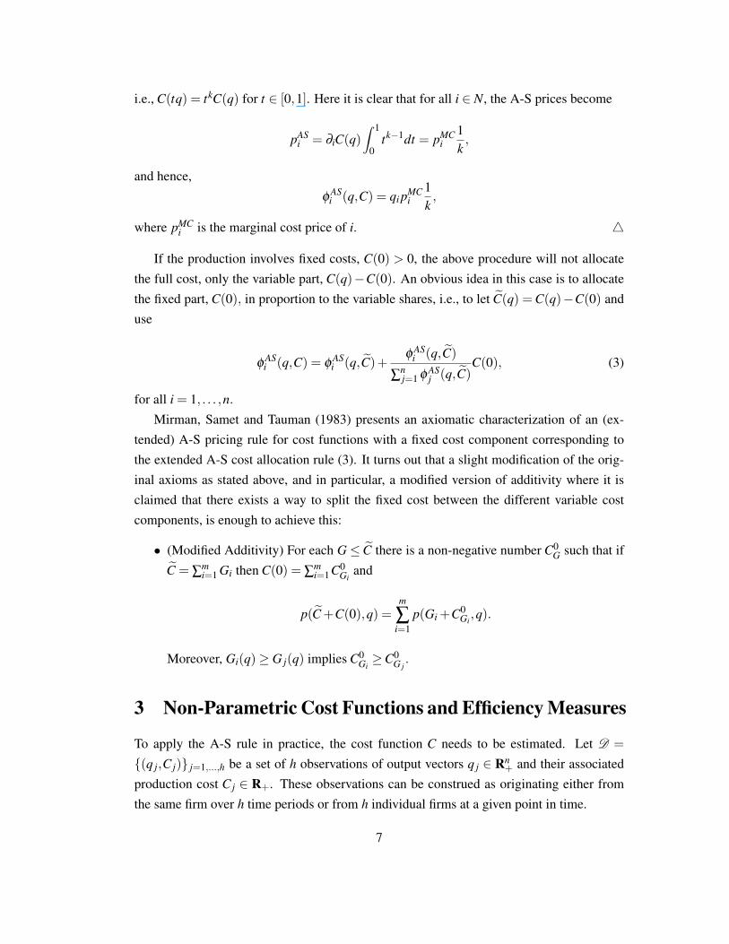
i.e., C(tq) = tkC(q) for t 2 [0,1]. Here it is clear that for all i 2 N, the A-S prices become

pASi = ∂iC(q)

Z 1

0tk�1dt = pMC

i1k,

and hence,f AS

i (q,C) = qi pMCi

1k,

where pMCi is the marginal cost price of i. 4

If the production involves fixed costs, C(0) > 0, the above procedure will not allocatethe full cost, only the variable part, C(q)�C(0). An obvious idea in this case is to allocatethe fixed part, C(0), in proportion to the variable shares, i.e., to let eC(q) =C(q)�C(0) anduse

f ASi (q,C) = f AS

i (q, eC)+f AS

i (q, eC)

Ânj=1 f AS

j (q, eC)C(0), (3)

for all i = 1, . . . ,n.Mirman, Samet and Tauman (1983) presents an axiomatic characterization of an (ex-

tended) A-S pricing rule for cost functions with a fixed cost component corresponding tothe extended A-S cost allocation rule (3). It turns out that a slight modification of the orig-inal axioms as stated above, and in particular, a modified version of additivity where it isclaimed that there exists a way to split the fixed cost between the different variable costcomponents, is enough to achieve this:

• (Modified Additivity) For each G eC there is a non-negative number C0G such that if

eC = Âmi=1 Gi then C(0) = Âm

i=1C0Gi

and

p(eC+C(0),q) =m

Âi=1

p(Gi +C0Gi,q).

Moreover, Gi(q)� G j(q) implies C0Gi

�C0G j.

3 Non-Parametric Cost Functions and Efficiency Measures

To apply the A-S rule in practice, the cost function C needs to be estimated. Let D =

{(q j,Cj)} j=1,...,h be a set of h observations of output vectors q j 2 Rn+ and their associated

production cost Cj 2 R+. These observations can be construed as originating either fromthe same firm over h time periods or from h individual firms at a given point in time.

7

Based on such a data set, a cost function may be estimated using a traditional paramet-ric approach where a given functional form is postulated and parameters associated withthis form are estimated. This approach is taken in numerous studies of cost functions, seee.g., Kumbhakar and Lovell (2000). However, using a standard parametric approach (typi-cally estimating parameters in log-linear or translog functional forms) may produce signifi-cantly biased estimates and provide invalid inference as shown in Delis, Iosifidi and Tsionas(2014), who argue that a semi-parametric smooth coefficient model yields better results. In-deed, to use various approaches for smoothing represents one way of obtaining well-definedA-S prices within a conventional econometric framework.

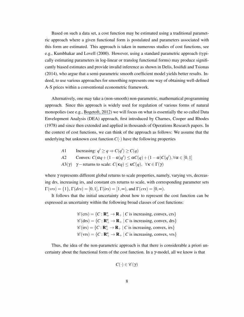
Alternatively, one may take a (non-smooth) non-parametric, mathematical programmingapproach. Since this approach is widely used for regulation of various forms of naturalmonopolies (see e.g., Bogetoft, 2012) we will focus on what is essentially the so called DataEnvelopment Analysis (DEA) approach, first introduced by Charnes, Cooper and Rhodes(1978) and since then extended and applied in thousands of Operations Research papers. Inthe context of cost functions, we can think of the approach as follows: We assume that theunderlying but unknown cost function C(·) have the following properties

A1 Increasing: q0 � q )C(q0)�C(q)A2 Convex: C(aq+(1�a)q0) aC(q)+(1�a)C(q0),8a 2 [0,1]A3(g) g � returns to scale: C(kq) kC(q), 8k 2 G(g)

where g represents different global returns to scale properties, namely, varying vrs, decreas-ing drs, increasing irs, and constant crs returns to scale, with corresponding parameter setsG(vrs) = {1}, G(drs) = [0,1], G(irs) = [1,•), and G(crs) = [0,•).

It follows that the initial uncertainty about how to represent the cost function can beexpressed as uncertainty within the following broad classes of cost functions:

C (crs) = {C : Rn+ ! R+ |C is increasing, convex, crs}

C (drs) = {C : Rn+ ! R+ |C is increasing, convex, drs}

C (irs) = {C : Rn+ ! R+ |C is increasing, convex, irs}

C (vrs) = {C : Rn+ ! R+ |C is increasing, convex, vrs}

Thus, the idea of the non-parametric approach is that there is considerable a priori un-certainty about the functional form of the cost function. In a g-model, all we know is that

C(·) 2 C (g)

8

i.e., we know that C(·) is increasing and convex, but otherwise we know nothing aboutthe cost function. Our a priori uncertainty does not stem from a lack of information abouta few parameters, as in a Coob-Douglas or a Translog statistical model. Rather, we lackinformation about all of the characteristics of the function except for a few general propertiessuch as its convexity and tendency to increase.

Now, to estimate a specific cost function from the available data D = {(q j,Cj)} j=1,...,h

we can rely on the the minimal extrapolation principle. We estimate the non-parametric costfunction as the largest function with these properties that is consistent with data in the sensethat Cj �C(q j), j = 1, . . . ,h, i.e., as

bC(q) := max{C(q) |C(·) 2 C (g),Cj �C(q j), j = 1, . . . ,h}

An important feature of the class of cost functions considered above is that a largest functionof this type actually exists – or, to put it differently, that the bC(·) defined above inherits theproperties from the C (g) class. This is shown for example in Bogetoft (1997).

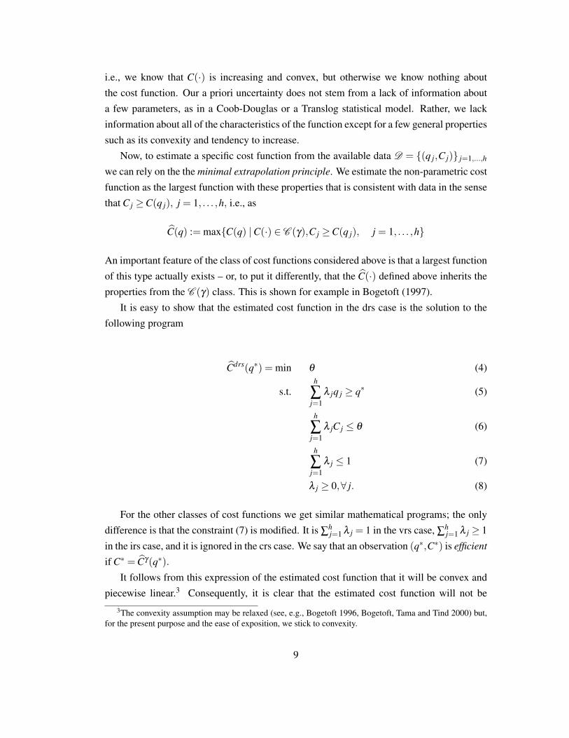
It is easy to show that the estimated cost function in the drs case is the solution to thefollowing program

bCdrs(q⇤) = min q (4)

s.t.h

Âj=1

l jq j � q⇤ (5)

h

Âj=1

l jCj q (6)

h

Âj=1

l j 1 (7)

l j � 0,8 j. (8)

For the other classes of cost functions we get similar mathematical programs; the onlydifference is that the constraint (7) is modified. It is Âh

j=1 l j = 1 in the vrs case, Âhj=1 l j � 1

in the irs case, and it is ignored in the crs case. We say that an observation (q⇤,C⇤) is efficientif C⇤ = bCg(q⇤).

It follows from this expression of the estimated cost function that it will be convex andpiecewise linear.3 Consequently, it is clear that the estimated cost function will not be

3The convexity assumption may be relaxed (see, e.g., Bogetoft 1996, Bogetoft, Tama and Tind 2000) but,for the present purpose and the ease of exposition, we stick to convexity.

9

differentiable in general. In fact, local non-differentiability of bC(q) may create problemswhen determining the A-S prices (and thereby the A-S cost shares) for specific data points.A problem which we return to in the next section.

Since we will also be concerned with cost allocation in the presence of inefficiency,we further introduce a few efficiency measures. In the spirit of Debreu (1951) and Farrell(1957) we can measure the efficiency of the observation (q⇤,C⇤) relative to the (estimated)cost function bC using the radial indexes,

Eq((q⇤,C⇤), bC) = max{q 2 R |C⇤ � bC(qq⇤)} 2 [1,•) (9)

and

Ec((q⇤,C⇤), bC) = min{q 2 R | qC⇤ � bC(q⇤)} 2 [0,1] (10)

By (9) we get that, given the cost level C⇤, the firm could have produced output levelEqq⇤ if it was efficient. By (10) we get that, given the output production q⇤, the firm couldhave produced at costs EcC⇤ if it was efficient. Under crs it is well known that4,

Ec((q⇤,C⇤), bCcrs) =1

Eq((q⇤,C⇤), bCcrs)(11)

4 Estimation of Aumann-Shapley Cost Shares

Following the approach in Hougaard and Tind (2009), calculation of A-S cost shares withrespect to an estimated cost function bC can be done using parametric programming.5 Indeed,the A-S prices (and hence cost shares) are easily determined as a finite sum of gradients ofthe linear pieces of bC along the line segment [0,q] weighted with the normalized length ofthe subintervals where bC has constant gradient.

Specifically, consider a given output vector q⇤ and a parameter value t 2 [0,1]. Now, we4see e.g., Bogetoft and Otto (2010).5See, e.g., Bazaraa, Jarvis and Sherali (1990).

10

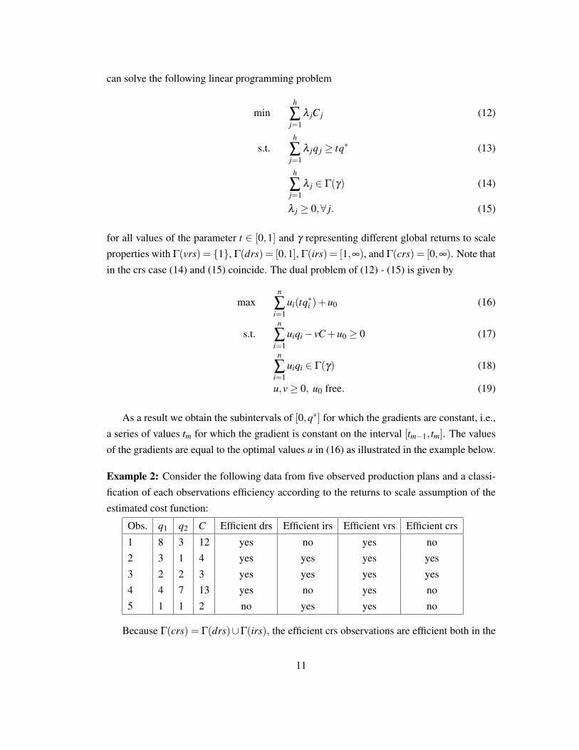
can solve the following linear programming problem

minh

Âj=1

l jCj (12)

s.t.h

Âj=1

l jq j � tq⇤ (13)

h

Âj=1

l j 2 G(g) (14)

l j � 0,8 j. (15)

for all values of the parameter t 2 [0,1] and g representing different global returns to scaleproperties with G(vrs) = {1}, G(drs) = [0,1], G(irs) = [1,•), and G(crs) = [0,•). Note thatin the crs case (14) and (15) coincide. The dual problem of (12) - (15) is given by

maxn

Âi=1

ui(tq⇤i )+u0 (16)

s.t.n

Âi=1

uiqi � vC+u0 � 0 (17)

n

Âi=1

uiqi 2 G(g) (18)

u,v � 0, u0 free. (19)

As a result we obtain the subintervals of [0,q⇤] for which the gradients are constant, i.e.,a series of values tm for which the gradient is constant on the interval [tm�1, tm]. The valuesof the gradients are equal to the optimal values u in (16) as illustrated in the example below.

Example 2: Consider the following data from five observed production plans and a classi-fication of each observations efficiency according to the returns to scale assumption of theestimated cost function:

Obs. q1 q2 C Efficient drs Efficient irs Efficient vrs Efficient crs1 8 3 12 yes no yes no2 3 1 4 yes yes yes yes3 2 2 3 yes yes yes yes4 4 7 13 yes no yes no5 1 1 2 no yes yes no

Because G(crs) = G(drs)[G(irs), the efficient crs observations are efficient both in the

11

drs and irs cases.Now, let q⇤ = (5,3) and define q = (q1(t), q2(t)) = (q⇤1t,q⇤2t) = (5t,3t). Since the es-

timated cost function differs under the four different returns to scale assumptions we get:bCdrs(5,3) = bCvrs(5,3) = 8.25, and bCcrs(5,3) = bCirs(5,3) = 7.

Solving (16)-(19) above we get

t obj. func., drs obj. func., irs obj. func., vrs obj. func., crs0 t < 0.2 1.25q1 +0.25q2 0q1 +0q2 +2 0q1 +0q2 +2 1.25q1 +0.25q2

0.2 t < 0.5 1.25q1 +0.25q2 q1 +0q2 +1 q1 +0q2 +1 1.25q1 +0.25q2

0.5 t < 0.77 1.43q1 +0.43q2 �0.71 1.25q1 +0.25q2 1.43q1 +0.43q2 �0.71 1.25q1 +0.25q2

0.77 t 1 1.25q1 +1.5q2 �2.5 1.25q1 +0.25q2 1.25q1 +1.5q2 �2.5 1.25q1 +0.25q2

First, consider the drs-case. From the above table we get Aumann-Shapley cost shares

xAS1 = 5⇥{1.25⇥0.5+1.43⇥ (0.77�0.5)+1.25⇥ (1�0.77)}= 6.49

xAS2 = 3⇥{0.25⇥0.5+0.43⇥ (0.77�0.5)+1.5⇥ (1�0.77)}= 1.76

Observe that xAS1 +xAS

2 = 8.25 which is equal to the objective function value of the aboveprogram when t = 1, as it should be. The third constraint of the primal problem (14) isbinding and receives in this case a non-zero dual variable value which is equal to the element-2.5 in the last row of the table. Again from the last row we see that the optimal dual variablecorresponding to the first element in the output vector is equal to 1.25. Multiplication of thisprice by the output quantity q1 = 5 gives the value of 6.25. The difference between xAS

1 andthis value is 0.23. The similar difference corresponding to the second element of the outputvector is -2.74. The two differences add to 2.5 (ignoring small rounding errors) which isequal to the value of the optimal dual variable corresponding to the convexity constraint, asit should be. In this way the dual variable for the convexity constraint is distributed on tothe values of the output vector.

Second, for the irs-case the Aumann-Shapley cost shares are (xAS1 ,xAS

2 ) = (4.63,0.38)which sum up to 5, while the value of the objective function is 7. The difference is dueto a fixed cost of 2, which is not surprising, since for t close to zero the objective functionis given by 0q1 + 0q2 + 2 (corresponding to a flat exterior facet). For the same reason, forvrs, we get (xAS

1 ,xAS2 ) = (4.87,1.39) which sum up to 6.25 while the value of the objective

function at this point is 8.25 (including the fixed cost of 2). The allocation is unchanged forany positive fixed cost since the gradients (A-S prices) are not affected by changes in thelevel of the whole cost possibility set: thus allocation of such fixed costs is naturally done

12

in proportion to the A-S prices as suggested below. Finally, in the crs-case there is no fixedcost, and the allocated cost shares are (xAS

1 ,xAS2 ) = (6.25,0.75) summing up to 7 exactly as

they should. Note that the gradients are the same for all values of t and can therefore bedirectly used as A-S prices. 4

In the vrs- and irs-cases, the above approaches does not work directly, as we saw inExample 2 above, since there may be fixed costs, i.e., bC(0)> 0. In this case we may proceedin two steps. First, we calculate the variable part of the cost function,

eC(q) = bC(q)� bC(0)

It is easy to show that when bC 2 C vrs, the variable part eC 2 C drs, and similarly when bC 2C irs, the variable part eC 2C drs. We can therefore use the variable part to determine A-S costshares and then, second, allocate the fixed costs in proportion to these as explained above,i.e., as

f ASi (q, bCvrs) = f AS

i (q, bCvrs � bCvrs(0))+f AS

i (q, bCvrs � bCvrs(0))

Ânj=1 f AS

j (q, bCvrs � bCvrs(0))bCvrs(0) (20)

for all i = 1, . . . ,n, and similarly for the irs-case.

Consider now again the drs- or crs-cases. Although the Hougaard and Tind (2009) ap-proach provides A-S prices for many production possibilities q, there are several limitationsof the approach. First of all, the approach only allocates the efficient cost (as do indeedany allocation method based on the cost function). Firms that are inefficient will thereforenot in general get a full allocation of their actual costs. Second, for the efficient firms, A-Sprices may not be a unique because of multiple dual solutions associated with the parametriclinear programming problem. Moreover for some efficient firms A-S prices may be zero.We will illustrate the latter problems below and suggest a solution to multiplicity (as men-tioned in the introduction the problem of zero A-S prices can in principle to solved usingthe ”extended facet” approach of Olesen and Petersen, 1996). The problem of inefficientproduction will be addressed in Section 5.

Example 3: Imagine that we only have one observation (q⇤,C⇤) and assume that the un-derlying cost function satisfy constant returns to scale. In this case, it is intuitively obvious,that we do not have enough information to allocate costs C⇤ onto the different outputs. Anexample with two outputs is illustrated in Fig. 1 below. Here q⇤ = (q⇤1,q

⇤2) = (1,1) and

13

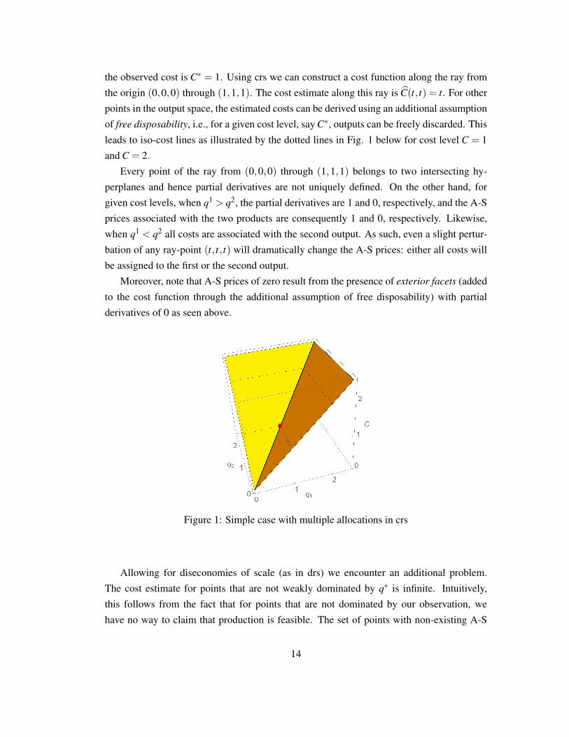
the observed cost is C⇤ = 1. Using crs we can construct a cost function along the ray fromthe origin (0,0,0) through (1,1,1). The cost estimate along this ray is bC(t, t) = t. For otherpoints in the output space, the estimated costs can be derived using an additional assumptionof free disposability, i.e., for a given cost level, say C⇤, outputs can be freely discarded. Thisleads to iso-cost lines as illustrated by the dotted lines in Fig. 1 below for cost level C = 1and C = 2.

Every point of the ray from (0,0,0) through (1,1,1) belongs to two intersecting hy-perplanes and hence partial derivatives are not uniquely defined. On the other hand, forgiven cost levels, when q1 > q2, the partial derivatives are 1 and 0, respectively, and the A-Sprices associated with the two products are consequently 1 and 0, respectively. Likewise,when q1 < q2 all costs are associated with the second output. As such, even a slight pertur-bation of any ray-point (t, t, t) will dramatically change the A-S prices: either all costs willbe assigned to the first or the second output.

Moreover, note that A-S prices of zero result from the presence of exterior facets (addedto the cost function through the additional assumption of free disposability) with partialderivatives of 0 as seen above.

Figure 1: Simple case with multiple allocations in crs

Allowing for diseconomies of scale (as in drs) we encounter an additional problem.The cost estimate for points that are not weakly dominated by q⇤ is infinite. Intuitively,this follows from the fact that for points that are not dominated by our observation, wehave no way to claim that production is feasible. The set of points with non-existing A-S

14

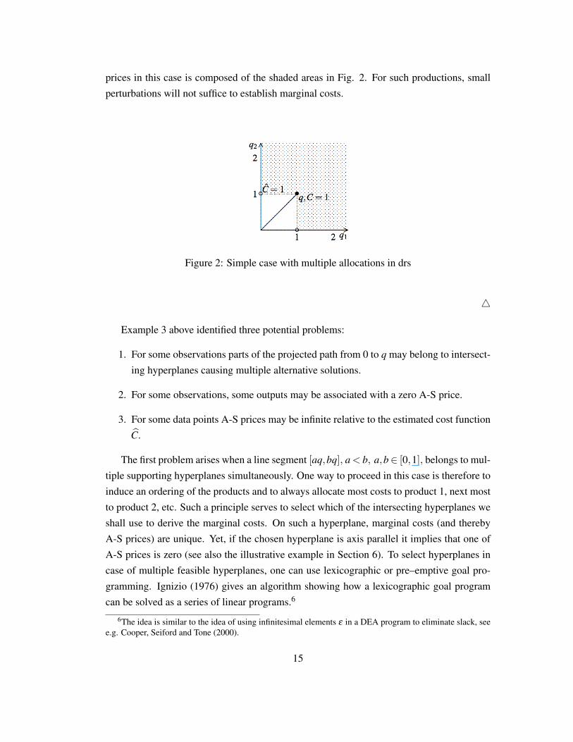
prices in this case is composed of the shaded areas in Fig. 2. For such productions, smallperturbations will not suffice to establish marginal costs.

Figure 2: Simple case with multiple allocations in drs

4

Example 3 above identified three potential problems:

1. For some observations parts of the projected path from 0 to q may belong to intersect-ing hyperplanes causing multiple alternative solutions.

2. For some observations, some outputs may be associated with a zero A-S price.

3. For some data points A-S prices may be infinite relative to the estimated cost functionbC.

The first problem arises when a line segment [aq,bq], a< b, a,b2 [0,1], belongs to mul-tiple supporting hyperplanes simultaneously. One way to proceed in this case is therefore toinduce an ordering of the products and to always allocate most costs to product 1, next mostto product 2, etc. Such a principle serves to select which of the intersecting hyperplanes weshall use to derive the marginal costs. On such a hyperplane, marginal costs (and therebyA-S prices) are unique. Yet, if the chosen hyperplane is axis parallel it implies that one ofA-S prices is zero (see also the illustrative example in Section 6). To select hyperplanes incase of multiple feasible hyperplanes, one can use lexicographic or pre–emptive goal pro-gramming. Ignizio (1976) gives an algorithm showing how a lexicographic goal programcan be solved as a series of linear programs.6

6The idea is similar to the idea of using infinitesimal elements e in a DEA program to eliminate slack, seee.g. Cooper, Seiford and Tone (2000).

15

To be more precise, consider the cost minimization problem associated with some outputvector q⇤:

min b (21)

s.t.h

Âj=1

l jq j � q⇤ (22)

h

Âj=1

l jCj b (23)

h

Âj=1

l j 1 (24)

l j � 0,8 j. (25)

where (24) is ignored if bCcrs is considered.The dual program is to find inputs and output prices v and u (u,v � 0) such that

max uq⇤+h (26)

s.t. v 1 (27)

�vCk +n

Âi=1

uiqki +h 0 8k = 1, . . . ,h (28)

h 0 (29)

where (29) becomes an equality requirement in the constant returns to scale case.We can reformulate this as a lexicographic goal programming problem by indicating the

sequence in which the objectives shall be optimized:

max P0(uq⇤+h)+P1(u1q⇤1)+P2(u2q⇤2)+ · · ·+Pn(unq⇤n) (30)

s.t. v 1 (31)

�vCk +n

Âi=1

uiqki +h 0 8k = 1, . . . ,h (32)

h 0 (33)

with the interpretation that we first optimize P0, then for fixed value of P0, we optimize P1,etc.

16

In practice, such an ordering of outputs may for instance be derived from various man-agerial priorities or pricing policies of the firm.

To ensure that all A-S prices are positive we may, for instance, use the extended facetapproach of Olesen and Petersen (1996, 2003), but this will not be pursued further in thepresent paper.7

Finally, the third problem, i.e., that data points may not have finite cost estimates, isaddressed by restricting attention to,

Q = {q⇤ 2 Rn+|9C⇤ : C⇤ � bC(q⇤)} (34)

i.e., to the set of feasible productions q given the observed data set D . In the drs-case, thiscan be rewritten as

Q = {q⇤ 2 Rn+|9C⇤ :

h

Âj=1

l jq j � q⇤,h

Âj=1

l jCj C⇤,h

Âj=1

l j 1, l j � 0,8 j} (35)

where Âhj=1 l j 1 is ignored in the crs-case.

5 Inefficient Production

We will now consider how firms with inefficient production can be handled in the contextof A-S cost allocation. Since A-S prices are only defined for efficient production we needspecific assumptions about firm behavior in order to link the observed inefficiency to someunderlying efficient counterpart. To do this transparently and in a consistent manner we willemploy the notion of rational inefficiency introduced in Bogetoft and Hougaard (2003).

The main idea behind the notion of rational inefficiency is that what appears as inefficientproduction may actually benefit the firm. In particular, it is suggested that inefficiency mayrepresent a form of indirect, on-the-job compensation to agents in the firm and thereforeserves an important purpose as alternative means of payment. Hence, it is often reasonableto assume that inefficiency may be the result of a deliberate (rational) choice by the firmand not just a consequence of ignorance, bad organization of processes, wrong incentivesetc. As such, we will generally think of firms as seeking not only to maximize profit byminimizing costs, but also to enjoy slack in the production process.8

7Using the extended facet approach would also solve the problem of infinite A-S prices.8For further discussion about the various types and origins of inefficiency, see e.g., Bogetoft and Hougaard

(2003).

17

Firms may introduce slack (inefficiency) on the input side as well as the output side. Inthe present cost context, the input side is represented by the aggregate (joint) cost and theintroduction of slack on the input side naturally corresponds to assuming that firms delib-erately allow for a constant fraction of overspending. The size of that fraction is revealedby the inefficiency level that the firm actually chose. This approach will be formalized inSubsection 5.1 below. In Subsection 5.2 we will subsequently consider the case where firmsintroduce slack on the output side. That is, for given costs, firms benefit from the lost (orrather self consumed) outputs. Specifically, we assume that firms actually produce at therevenue maximizing point (given output prices or preference weights set by a regulator)and when we observe something else we can directly infer the preferred slack mix by com-parison with the allocatively efficient output mix. Thus, according to this assumption therelevent A-S prices are those associated with revenue maximizing production given (q⇤,C⇤)

and estimate bC. These A-S prices will generally differ from the preference weights set bythe regulator and reflect the internal (unit) production costs of the firm.

Finally, note that our approach, and associated results, do not depend on the way weestimate the empirical cost function.

5.1 Cost inefficiency

The fundamentals are the observed output-cost data (q⇤,C⇤) 2 D and the associated (esti-mated) cost function bC. Note that C⇤ � bC(q⇤) by definition of bC. A strict inequality meansthat the firm is inefficient.

One way to think of inefficiency is simply as an excess use of inputs. Instead of theminimal cost bC(q⇤), the firm has actually chosen to spend C⇤. Following the notion ofrational inefficiency we find it reasonable to assume that this tendency to use extra costs isnot restricted to the particular output level q⇤, i.e., that the firm would use a similar share ofexcess resources for any other production level as well. Indeed, if there would be efficiencygains from changing the size of production a rational firm would already have have doneso. Note that efficient firms have revealed that they do not gain utility from excess use ofresources.

Assumption 1: (Rational Cost Inefficiency) An inefficient firm with observed output-costcombination (q⇤,C⇤), in effect, faces a cost function

q 7! 1Ec((q⇤,C⇤), bC)

bC(q)

where Ec is the cost efficiency score given by (10).

18

Conceptually this means that we see the firm as deliberately spending a fraction (1�Ec((q⇤,C⇤), bC)) in excess of what is necessary in order to produce any level of output q.

The idea that inefficiency shows up as a general scaling of the costs is convenient in thecontext of A-S pricing since in general, A-S prices are linear in the cost level, i.e.,

pAS(q,aC) = a pAS(q,C), (36)

for a 2 R+.9

Assumption 1 allows us to use the Aumann-Shapley rule in case of inefficient productionin a straightforward way.

Proposition 1: Consider a set of observations D with specific inefficient observation (q⇤,C⇤).Given Assumption 1, we have for all outputs i = 1, . . . ,n, that,

f ASi (q⇤, bC

Ec ) = 1Ec f AS

i (q⇤, bC)

= f ASi (q⇤, bC)+

f ASi (q⇤,bC)

Ânj=1 f AS

j (q⇤,bC)(1�Ec)C⇤.

Proof: The first equality follows from Assumption 1 and (36). Consider the second equalityand a given output i. We have that

1Ec f AS

i (q⇤, bC) =C⇤

bC(q⇤)f AS

i (q⇤, bC) = (1+(1�Ec)C⇤

bC(q⇤))f AS

i (q⇤, bC) =

f ASi (q⇤, bC)+

f ASi (q⇤, bC)

Ânj=1 f AS

j (q⇤, bC)(1�Ec)C⇤

since Ânj=1 f AS

j (q⇤, bC) = bC(q⇤) by budget-balance. Q.E.D.

By Proposition 1 we see that focussing on cost efficiency (as in Assumption 1) is indeednatural since it opens up for an alternative way of looking at the problem: in fact, it givesthe same result as if we were assuming that the level of cost inefficiency for output vectorq⇤ can be construed as a general fixed cost F = (1�Ec)C⇤ in production. As such, we canalternatively analyze the particular situation given by observation (q⇤,C⇤) as if a fixed costF = (1�Ec)C⇤ had been added to the cost function such that the efficient cost of any levelq is given by bC(q)+F .

9See e.g., Mirman and Tauman (1982).

19

Proposition 1 shows that scaling A-S cost shares of the cost efficient production bC(q⇤)by a factor 1/Ec is tantamount to splitting the fixed cost of inefficiency F in proportion tothese A-S cost shares and add this to the cost shares of cost efficient production.

The advantage of this result is furthermore that it works well with the way we handledfixed costs C(0) in the case of vrs and irs technologies in Section 4. Here we also allocatedfixed cost in proportion to the variable cost A-S shares. By straightforward combination of(20) and Proposition 1, we therefore obtain the following result.

Corollary 1: Consider a set of observations D with a corresponding minimal extrapolationprinciple cost function bCg , where g is vrs, irs, drs or crs. Let

eCg = bCg � bCg(0)

be the variable part of the cost function, and consider a specific inefficient observation(q⇤,C⇤). Given Assumption 1, we have for all outputs i = 1, . . . ,n, that,

f ASi (q⇤, bCg

Ec ) = 1Ec f AS

i (q⇤, bCg)

= f ASi (q⇤, eCg)+

f ASi (q⇤,eCg )

Ânj=1 f AS

j (q⇤,eCg )[(1�Ec)C⇤+ bCg(0)].

where Ec is the cost efficiency of (q⇤,C⇤) with respect to eCg .

In the case of crs, we know that cost efficiency Ec is the inverse of output efficiencyEq. We can therefore also make an alternative interpretation of the A-S cost shares withinefficiency. We record this as a Corollary.

Corollary 2: Consider a set of observations D with specific inefficient observation (q⇤,C⇤).Given Assumption 1, in the crs-case we have that

f AS(q⇤, bCcrs

Ec ) = 1Ec f AS(q⇤, bCcrs)

= Eqf AS(q⇤, bCcrs)

= f AS(Eqq⇤, bCcrs).

Proof: By Assumption 1 and (36) we have

f AS(q⇤,a bCcrs) = pAS(q⇤,a bCcrs)q⇤ = a pAS(q⇤, bCcrs)q⇤ = af AS(q⇤, bCcrs).

Thus, the first equality follows from the fact that bCcrs(q⇤) = EcC⇤. The second equalityfollows from (11). The third equality follows from the fact that pAS(q,Ccrs) is constant (and

20

equal to the marginal cost): Hence, we have that f AS(Eqq⇤, bCcrs) = Eqq⇤pAS(Eqq⇤, bCcrs) =

Eqq⇤pAS(q⇤, bCcrs) = Eqf AS(q⇤, bCcrs). Q.E.D.

In other words, the A-S cost shares of inefficient production can be found by multiplyingthe A-S cost shares of the corresponding efficient production with the output efficiency scoreEq (given by (9)) or equivalently the inverse of the cost efficiency score Ec (given by (10)).Moreover, it does not matter whether we allocate the actual cost C⇤ using A-S prices relatedto q⇤ and scale up with a factor 1/Ec =Eq or the A-S-prices related to the efficiency adjustedoutput level Eqq⇤ directly. Indeed, when the estimated cost function has constant returns toscale, the A-S-prices are the same along the entire ray through 0 and q⇤.

5.2 Output Inefficiency

We now consider the case where firms introduce slack (inefficiency) on the output side. Themain postulate here is that firms benefit from self consumed outputs, broadly interpreted.Let us assume that a firm with output-cost profile (q⇤,C⇤) is actually producing some otherefficient output level q � q⇤, but that only q⇤ is observed since the firm itself consumesq�q⇤. In such cases, it would be natural to allocate costs based on the efficient productionlevel q rather than the observed level q⇤.

The problem with this line of thinking is of course that q is unobserved. Yet, by Propo-sition 1 and Corollary 1 in Bogetoft and Hougaard (2003), it is proved that a firm withpreferences for both profit and slack will choose q as the allocatively efficient output mix.

Specifically, assume that output prices are given by the price vector p. This may bemarket prices or as in the empirical example provided in the next section, the prices (prefer-ence weights) set by a regulator. Given these prices, a rationally inefficient firm will chooseoutput vector q as the allocatively efficient solution qAE to

maxq

p ·q (37)

s.t. bC(q)C⇤ (38)

The intuition behind this result is that for a given cost level, the firms choice problem isreally one of choosing the underlying production q so as to maximize revenue. This leavesthe firm with maximal possibility to enjoy slack q�q⇤.

Of course, if this vector difference is not non-negative in all dimensions, we can saythat the firm has not behaved fully rational. Our assumption concerning rational output

21

inefficiency can therefore be formulated as follows:

Assumption 2: (Rational Output Inefficiency) Given an output price vector p, an inefficientfirm with observed output-cost combination (q⇤,C⇤)) chooses the underlying productionplan q such as to maximize revenue subject to q � q⇤, i.e., as the solution to,

maxq

p ·q (39)

s.t. bC(q)C⇤ (40)

q � q⇤ (41)

Let qAE(p, bC;q⇤) solve the above programming problem.Assumption 2 implies that when we observe output level q⇤, there is an underlying pro-

duction plan qAE(p, bC;q⇤), which the rational firm actually did produce (before consumingslack internally) and, which should therefore be used when determining the A-S prices andthe associated A-S cost allocation.

To illustrate the idea, imagine a firm that produces q but internally consumes a largeshare of the first output q1. It may for example be a baker that produces multiple types ofbread but only consumes one of them himself. Now, if we allocate costs according to theobserved production q⇤ (i.e., what is left of q after his own consumption), the cost of thebakers consumption will effectively be spread over all breads, but if we allocate the costaccording to q, it will be allocated to the first type of bread. Another example may be afirm that have quality issues in the production process. Assume that a large share of the firstproduct generally have to be discarded. If we allocate cost according to the set of productsof good quality, all products will share the costs of the quality issue in the production of thefirst product. If instead we take the rational inefficiency approach, we will allocate the extracosts to the first product.

We now record the straightforward consequence of Assumption 2 with respect to A-Scost allocation.

Proposition 2: Consider a set observations D with a corresponding minimal extrapolationprinciple cost function bCg , where g is vrs, irs, drs or crs, and consider a specific inefficientfirm with observation (q⇤,C⇤). Given Assumption 2, we have that,

f AS(q⇤, bCg) = pAS(qAE(p, bCg ;q⇤), bCg)qAE(p, bCg ;q⇤).

22

for output price vector p.

Notice that with a non-parametric estimation of the cost function there may be caseswith multiple allocatively efficient points for a given observation. The problem is of coursethat these points typically will have different A-S prices. In such cases we therefore suggestto apply the ordering of outputs similarly to the way we addressed the issue of multiplesupporting hyperplanes for given efficient point in Section 4 above.

6 An Illustrative Example

Water companies are by and large natural monopolies that usually provide two services,namely the production of water and the distribution of water to households and firms. Thewater network requires large infrastructure investments making it economically optimal toonly have one distribution network in each area. Water from different sources can in the-ory be distributed using the same network. Much like the electricity sector, it is thereforepossible to have competition among producers of water and to reduce the natural monopolyscope to the distribution. Still, preservation of ground water reserves and quality concernshave in many jurisdictions led to natural geographical monopolies in water production aswell.

In most countries, the regulation of water companies has been low powered, typicallybased on a cost plus regime. This seems to be changing. In recent years there have beenseveral attempts to move towards a more high powered regime like a revenue cap similarto the regulation that has long been prominent for electricity distribution companies in forexample Europe, cf., Bogetoft (2012).

When the typical operators are responsible for both production and distribution of wa-ter, it is interesting to allocate total costs among these activities. This may for exampleguide which tariffs different consumer types shall pay, and it may guide the access fees anincumbent waterworks with both production and distribution can charge external producers.

The first high powered regulation of Danish waterworks was introduced in 2012. Theregulation is a benchmarking based revenue cap regulation. The benchmarking model is acrs DEA model with one main output, net volume. The net volume is the sum of several netvolume elements that are designed to measure the amount of activities in different areas.

In the following we will use the 2011 data used to make the 2012 regulation and illustratehow this data can be used to allocate cost between water production and water distribution.There are 210 waterworks in the data set, and the amount of water production and waterdistribution activities (measured in netvolumes) as well as the operating costs (measured in

23

DKK) are summarized in Table 1 below.

Mean Std. dev Min MaxWater Production, q1 2888260.25 8396426.53 0.00 109821313.10Water Distribution, q2 3916069.50 7607266.44 571.20 74436410.28Cost, C 7026759.82 15449475.55 55073.21 184313172.69

Table 1: Descriptive statistics.

6.1 The Estimated Cost Function

We will focus on non-parametric estimation of the empirical cost functions in case of crs (asassumed by the Danish regulator) and drs for the sake of illustration. That is, the estimatedcost function is given by the program (4)-(8) (in case of drs), excluding (7) in case of crs.

In case of crs we find only three efficient waterworks: Hjerting Vandværk Amba, BjøvlundVandværk, and, Nordenskov Vandværk. These three observations span the convex cone ofthe estimated cost function. Under drs there turns out to be additionally seven efficientwaterworks spanning the cost function, all listed in Table 2 below.

Name Water Production, q1 Water Distribution, q2 Cost, C

KE Vand A/S 109821313.10 74436410.28 184313172.69Vandcenter Syd A/S 19986564.36 34731824.80 47964952.93Sjælsø Vand A/S 15061136.50 109336.00 14367705.59Hjerting Vandværk Amba 835293.97 3760657.20 1882561.43Bjøvlund Vandværk 1179982.57 188126.60 737445.92Nordenskov Vandværk 590749.90 593366.00 436994.91Helle Vest Vandværk 1163503.15 1068388.20 869824.16Vestforsyning Vand A/S 8307093.20 13291457.40 15500628.99Arhus Vand A/S 1163503.15 1068388.20 869824.16Hjørring Vandselskab A/S 8586097.67 10675079.00 12526393.57

Table 2: Efficient waterworks (drs).

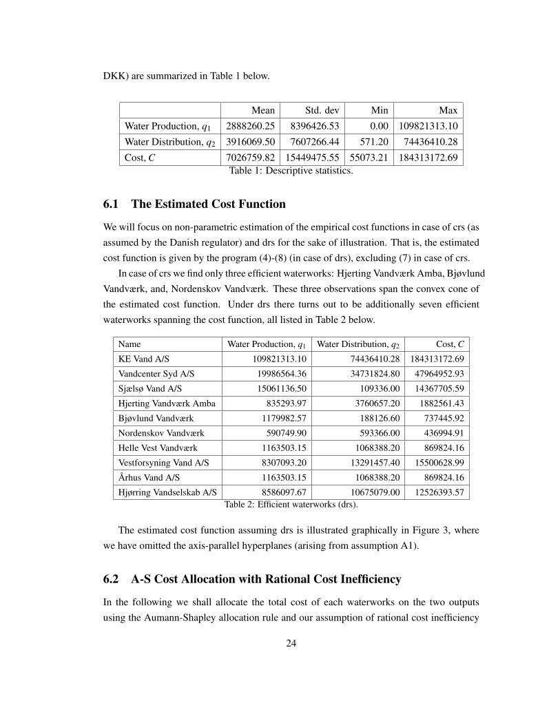
The estimated cost function assuming drs is illustrated graphically in Figure 3, wherewe have omitted the axis-parallel hyperplanes (arising from assumption A1).

6.2 A-S Cost Allocation with Rational Cost Inefficiency

In the following we shall allocate the total cost of each waterworks on the two outputsusing the Aumann-Shapley allocation rule and our assumption of rational cost inefficiency

24

0 100000000q1

0

70000000

q2

0

180000000

C

Figure 3: bCdrs based on the data set

(Assumption 1). In all cases the associated Aumann-Shapley prices are calculated usingMatlab to solve the program (16)-(19) where t is gradually increased from 0 to 1. Sincethe constraints remain unchanged when going through the individual waterworks (only theobjective function varies) we can improve the computational speed by first finding the setof vertices (extreme points of the frontier) defined by the intersecting hyperplanes givenby the constraints. For each of the waterworks we then evaluate the objective function onall those vertices (since the solution will always lie in a vertex). In this way we obtaintwo advantages; first, we can easily detect how many hyperplanes the production plan inquestion lies on, and second, we get solutions significantly faster than by solving the LPproblem for each of the waterworks.

Turning to the drs-case: Obviously no waterworks will face the problem of infinite A-Sprices since they are all included in the estimation of the cost function. Three of the efficientwaterworks face the problem of multiple alternative solutions. For instance this is the casefor Nordenskov Vandværk, which is illustrated in Figure 4.

The green line lies on two hyperplanes simultaneously, and the two possible candidatesfor A-S prices are pAS = (0.6033,0.1338) and pAS = (0.3050,0.4329), respectively. In bothcases all costs are allocated to the both outputs, because Nordenskov Vandværk is efficient.To choose between the two possible A-S price candidates one can define an exogenousordering of outputs as described in section 4.

If most costs are allocated to output 1 and the A-S allocation becomes:xAS

1 = 356405.15xAS

2 = 80589.76

25

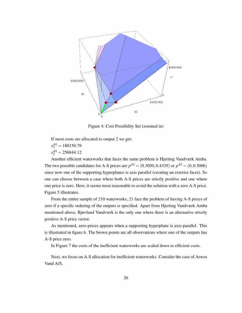
Figure 4: Cost Possibility Set (zoomed in)

If most costs are allocated to output 2 we get:xAS

1 = 180150.79xAS

2 = 256844.12Another efficient waterworks that faces the same problem is Hjerting Vandværk Amba.

The two possible candidates for A-S prices are pAS = (0.3050,0.4329) or pAS = (0,0.5006)since now one of the supporting hyperplanes is axis parallel (creating an exterior facet). Soone can choose between a case where both A-S prices are strictly positive and one whereone price is zero. Here, it seems most reasonable to avoid the solution with a zero A-S price.Figure 5 illustrates.

From the entire sample of 210 waterworks, 21 face the problem of having A-S prices ofzero if a specific ordering of the outputs is specified. Apart from Hjerting Vandværk Ambamentioned above, Bjøvlund Vandværk is the only one where there is an alternative strictlypositive A-S price vector.

As mentioned, zero-prices appears when a supporting hyperplane is axis-parallel. Thisis illustrated in figure 6. The brown points are all observations where one of the outputs hasA-S price zero.

In Figure 7 the costs of the inefficient waterworks are scaled down to efficient costs.

Next, we focus on A-S allocation for inefficient waterworks. Consider the case of ArwosVand A/S.

26

Figure 5: Cost Possibility Set (zoomed in)

0

9000000

q1

0

9 000000

q2

0

9 000000

C

Figure 6: Cost Possibility Set

27

0

9000000

q10

9 000000

q2

0

9 000000

C

Figure 7: Cost Possibility Set

Name Water Production Water Distribution CostArwos Vand A/S 2869541.62 3541004.80 8218777.91

First we find the A-S prices in the (hypothetical) situation where the production is costefficient (i.e., with a total cost of 3679269.17). These prices are pAS = (0.7066,0.4664) andthe A-S allocation of (efficient) cost hence becomes;

xAS1 = 2027728.22

xAS2 = 1651540.96

The remaining costs are inefficiency costs, which are allocated in proportion to the A-Scost shares (cf., Proposition 1). For instance output 1 gets allocated an additional ineffi-ciency cost of

f AS1

f AS1 +f AS

2(C⇤ �C⇤Ec) =

2027728.222027728.22+1651540.96

(8218777.91�3679269.17)

= 2734589.54.

The final allocation thus becomes:xAS

1 = 4529553.86xAS

2 = 3689224.05In the drs-case there are 200 inefficient waterworks with an average cost inefficiency of

28

2262943.92 corresponding to 50.95 % of the total costs. No inefficient waterworks face theproblem of multiple A-S prices, and on average 40.36 % of the total costs are allocated onoutput 1 and 59.64 % on output 2.

6.3 A-S Cost Allocation with Rational Output Inefficiency

Turning to output inefficiency, we shall assume that the relevant output prices are the samefor both outputs. The regulator effectively construct the total net volume by adding the netvolume of production and distribution. This means that the waterworks will use 1:1 priceson the outputs when they try to “play the regulation”. Using 1:1 prices, we can calculate theproductions that maximize the revenue permitted by the regulator.

According to Assumption 2, the revenue maximizing allocatively efficient productionplan is the underlying production plan chosen by the waterworks. The difference betweenthis production plan and the observed production plan is the slack ”consumed” by the wa-terworks.

In the case of Arwos we find the allocatively optimal production as

(q1,q2,C) = (5449306.06,7876775.60,8218777.91),

solving (37).The corresponding A-S prices are pAS = (0.8173,0.4780)) and hence the resulting A-S

cost allocation becomes:xAS

1 = 4453671.04xAS

2 = 3765120.09which is rather close to the allocation found by considering cost inefficiency (as is indeed

the case for the ”average observation”, cf., table below). The graphical interpretation ofinput inefficiency and rational output inefficiency is illustrated in figure 8 for Arwos.

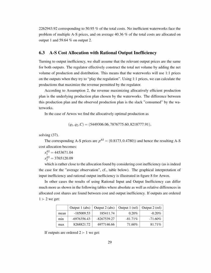
In other cases the results of using Rational Input and Output Inefficiency can differmuch more as shown in the following tables where absolute as well as relative differences inallocated cost shares are found between cost and output inefficiency. If outputs are ordered1 � 2 we get:

Output 1 (abs) Output 2 (abs) Output 1 (rel) Output 2 (rel)mean -185009.53 185411.74 0.20% -0.20%min -6976356.43 -8267539.27 -81.71% -71.60%max 8268821.72 6977146.66 71.60% 81.71%

If outputs are ordered 2 � 1 we get:

29

Figure 8: Arwos, inefficiency

Output 1 (abs) Output 2 (abs) Output 1 (rel) Output 2 (rel)mean -182594.78 182996.98 1.01% -1.01%min -6976356.43 -8267539.27 -81.71% -71.60%max 8268821.72 6977146.66 71.60% 81.71%

Consider, for instance, the waterworks Mariager Vand Amba, which has the outputcost profile (q1,q2,C) = (150599.20,811534.80,642263.95). When using input cost in-efficiency we see that the same output could be obtained at cost 406249.24, and the finalallocation of actual cost (for both orderings of outputs) is:

xAS1 = 0

xAS2 = 642263.95

This highlight the problem of allocating zero costs. If instead we use the rational outputinefficiency approach with price ratio 1:1, we get that the following allocatively efficientpoint: (q1,q2,C) = (862377.82,818645.02,642263.95). The final allocation (for both or-derings of outputs) therefore is:

xAS1 = 524813.62

xAS2 = 117443.18

The absolute difference here is 0�524813.62=�524813.62 for output 1 and 642263.95�117443.18 = 524820.77 for output 2 (the slight difference is caused by rounding errors),corresponding to relative differences of �81.71% and 81.71% respectively. When using

30

rational output inefficiency no waterworks face the problem of allocating zero costs.It is not surprising, as such, that the difference between A-S cost shares with respect

to cost and output efficiency can be rather big. Clearly, when deviating from an overallassumption of constant returns to scale, the efficiency of certain observations can be verydifferent in cost and output space respectively. In a specific application, like the one above,the choice between cost (input) or output orientation is in many ways a counterpart of thesimilar type of choice in a conventional efficiency analysis: if focus is on cost savings andinefficiency is mainly due to ”bad” utilization of resources it seems natural to allocate costsusing A-S prices associated with cost minimization; if focus is on quality issues or otherforms of ”slack” allocation in production it seems natural to employ A-S prices associatedwith output efficient production. As such the decision is ad hoc and related to the data set athand.

7 Final Remarks

In the efficiency measurement literature it is well recognized that the non-parametric es-timation of the efficient frontier (of either the production or cost function) is sensitive tosmall changes in the data since the frontier is spanned by ”extreme” observations. Obvi-ously non-parametric estimation of A-S prices inherits this sensitivity as the gradients onthe projected path (from 0 to q) may change dramatically moving from one efficient facet ofthe convex polyhedral to another. The remedy is usually to bootstrap the estimated function,see e.g. Simar and Wilson (1998). The sensitivity of A-S price estimates and the use ofbootstrapping techniques is a topic we leave for future research

References

[1] Asmild, M, P. Bogetoft and J.L. Hougaard (2009), Rationalising DEA estimated inef-ficiencies, Journal of Business Economics ZfB, 87- 97.

[2] Asmild, M, P. Bogetoft and J.L. Hougaard (2013), Rationalising inefficiency: Staff utilisation in branches of a large Canadian bank, Omega, 41, 80-87.

[3] Aumann, R and L. Shapley (1974), Values of Non-atomic Games, Princeton University Press.

[4] Banker, R.D. (1999), Studies in Cost Allocation and Efficiency Evaluation, UMI-Press.

31

[5] Banker R.D., A. Charnes and W.W. Cooper (1984), Some models for estimating tech-nical and scale inefficiencies in Data Envelopment Analysis, Management Science, 30, 1078-1092.

[6] Bazaraa, M.S., J.J. Jarvis and H.D. Sherali (1990), Linear Programming and Network Flows (2’ed.), Wiley.

[7] Billera, L.J. and C. Heath (1982), allocation of shared costs: a set of axioms yielding a unique procedure, Mathematics of Operations Research, 7, 32-39.

[8] Billera, L.J., C. Heath and J. Raanan (1978), Internal telephone billing rates - a novel application of non-atomic game theory, Operations Research, 26, 956-965.

[9] Bjørndal, M. and K. Jornsten (2005), An Aumann-Shapley approach to cost allocation and pricing in a supply chain; In Koster and Delfman (eds), Supply Chain Manage-ment, CBS-Press, p. 182-198.

[10] Bogetoft, P. (1996), DEA on relaxed convexity assumptions, Management Science, 42,457-465.

[11] Bogetoft, P. (1997), DEA-Based Yardstick Competition: The Optimality of Best Prac-tice Regulation, Annals of Operations Research, 73, 277-298.

[12] Bogetoft, P., and J.L. Hougaard (2003), Rational inefficiency, Journal of Productivity Analysis, 20, 243-271.

[13] Bogetoft, P. and L. Otto (2010), Benchmarking with DEA, SFA and R, Springer New York.

[14] Bogetoft, P. J.M. Tama and J. Tind (2000), Convex input and output projections of nonconvex production possibility sets, Management Science, 46, 858-869.

[15] Bogetoft, P. (2012), Performance Benchmarking: Measuring and Managing Perfor-mance, Springer New York.

[16] Castano-Pardo, A. and A. Garcia-Diaz (1995), Highway cost allocation: An applica-tion of the theory of non-atomic games, Transportation Research, 29, 187-203.

[17] Charnes, A. W.W. Cooper and E. Rhodes (1978), Measuring the efficiency of decision making units, European Journal of Operational Research, 2, 429-444.

32

[18] Cooper, W.W., L.M. Seiford and K. Tone (2000), Data Envelopment Analysis: A Com-prehensive Text with Models, Applications, References and DEA-Solver Software, Kluwer Academic Publishers, Boston.

[19] Delis, M.D., M. Iosifidi and E. Tsionas (2014), On the estimation of marginal cost, Operations Research, 62, 543-556.

[20] Friedman, E. and H. Moulin (1999), Three methods to share joint costs or surplus, Journal of Economic Theory, 87, 275-312.

[21] Haviv, M. (2001), The Aumann-Shapley price mechnism for allocating congestion costs, Operations Research Letters, 29, 211-215.

[22] Hougaard, J.L. (2009), An Introduction to Allocation Rules, Springer.

[23] Hougaard, J.L. and J. Tind (2009), Cost allocation and convex data envelopment, Eu-ropean Journal of Operational Research, 194, 939-947.

[24] Ignizio, J.P. (1976), Goal Programming and Extensions, Lexington Books, Lexington, MA.

[25] Mirman, L. and Y. Tauman (1982), Demand compatible equitable cost sharing prices, Mathematics of Operations Research, 7, 40-56.

[26] Mirman, L., Y. Tauman and I. Zang (1985a), On the use of game-theoretic concepts in cost accounting; Chapter 3 in Young (Editor) Cost Allocation: Methods, Principle, Applications, North Holland.

[27] Mirman, L., Y. Tauman and I. Zang (1985b), Supportability, sustainability and subsidy-free prices, RAND Journal of Economics, 16, 114-126.

[28] Mirman, L., D. Samet and Y. Taumann (1983), An axiomatic approach to allocation of a fixed cost through prices, Bell Journal of Economics, 14, 139-151.

[29] Olesen, O.B. and N.C. Petersen (1996), Indicators of ill-conditioned data sets and model specification in Data Envelopment Analysis: an extended facet approach, Man-agement Science, 42, 205-219.

[30] Olesen, O.B. and N.C. Petersen (2003), Identification and use of efficient faces and facets in DEA, Journal of Productivity Analysis, 20, 323-360.

33

[31] Samet, D., Y. Tauman and I. Zang (1984), An application of the Aumann-Shapley prices for cost allocation in transportation problems, Mathematics of Operations Re-search, 9, 25-42.

[32] Spulber, D.F. (1989), Regulation and Markets, MIT-Press.

[33] Simar, L. and P. Wilson (1998), Sensitivity analysis of efficiency scores: How to boot-strap in non-parametric frontier models, Management Science, 44, 49-61.

[34] Tsanakas, A. and C. Barnett (2003), Risk capital allocation and cooperative pricing of insurance liabilities,Insurance: Mathematics and Economics, 33, 239-254.

[35] Young, H.P. (1985), Producer incentives in cost allocation, Econometrica, 53, 757-765.

34