“Applications of trajectory statistical methods (TSM)” Dr PEDRO SALVADOR Department of...
45
“Applications of trajectory statistical methods (TSM)” Dr PEDRO SALVADOR Department of Environment - CIEMAT, Madrid, Spain Regional Training Course on Source Identification and Apportionment of Air Particulate Matter (APM), Sacavem, Portugal, 2 – 6 June 2014
-
Upload
alfonso-goldrich -
Category
Documents
-
view
214 -
download
0
Transcript of “Applications of trajectory statistical methods (TSM)” Dr PEDRO SALVADOR Department of...
“Applications of trajectory statistical methods (TSM)”
Dr PEDRO SALVADOR
Department of Environment - CIEMAT, Madrid, Spain
Regional Training Course on Source Identification and Apportionment of Air Particulate Matter (APM), Sacavem, Portugal, 2 – 6 June 2014

• Learning SURFER skills
• Cluster Analysis: Cape Verde, a case study
• RTA-CPF: Cape Verde, a case study
• Learning SURFER skills
• Cluster Analysis: Cape Verde, a case study
• RTA-CPF: Cape Verde, a case study
STRUCTURE OF THE PRESENTATIONSTRUCTURE OF THE PRESENTATION
• The algorithms of the TSM were programmed with FORTRAN77
• The final data treatment was performed with EXCEL
• The graphical representation of the products (trajectories, meteorological fields, RTA maps,
RCF…) were performed with SURFER
• The algorithms of the TSM were programmed with FORTRAN77
• The final data treatment was performed with EXCEL
• The graphical representation of the products (trajectories, meteorological fields, RTA maps,
RCF…) were performed with SURFER
MAIN COMPUTER TOOLSMAIN COMPUTER TOOLS

1- LEARNING SURFER SKILLS
SURFER is a comercial software for Windows
SURFER is a grid-based contouring and 3-D surface plotting images
LEARNING SURFER SKILLS
SURFER will help us to:
• Plot back-trajectories over a regular geographic grid
• Create and represent a regularly spaced grid of meteorological variables
• Create and represent interpolated maps from a regularly spaced grid of variables
• Represent CPF or Concentration Fields on a regularly spaced grid
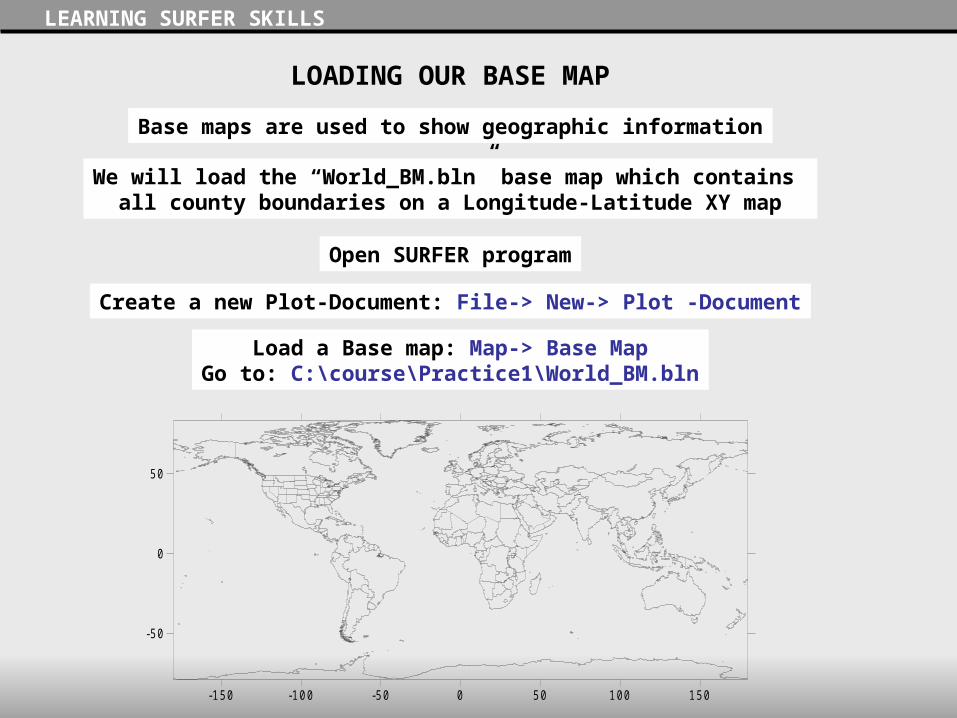
LOADING OUR BASE MAP
Open SURFER program
LEARNING SURFER SKILLS
Create a new Plot-Document: File-> New-> Plot -Document
Load a Base map: Map-> Base MapGo to: C:\course\Practice1\World_BM.bln
Base maps are used to show geographic information
We will load the “World_BM.bln” base map which contains all county boundaries on a Longitude-Latitude XY map
-150 -100 -50 0 50 100 150
-50
0
50
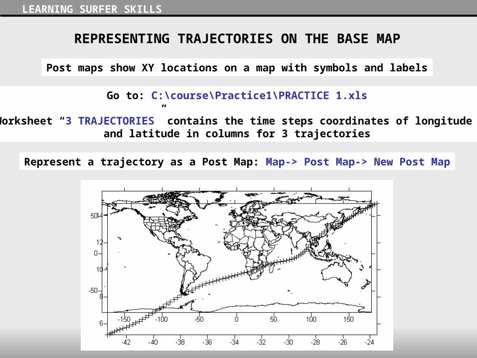
REPRESENTING TRAJECTORIES ON THE BASE MAP
LEARNING SURFER SKILLS
Go to: C:\course\Practice1\PRACTICE 1.xls
Worksheet “3 TRAJECTORIES” contains the time steps coordinates of longitude and latitude in columns for 3 trajectories
Represent a trajectory as a Post Map: Map-> Post Map-> New Post Map
Post maps show XY locations on a map with symbols and labels

REPRESENTING TRAJECTORIES ON THE BASE MAP
LEARNING SURFER SKILLS
The properties of the trajectory can be changed here (symbol and size of the time steps, coordinates of other trajectories…)
Select the Post Map in the left column, where all the objects of your map are displayed
REPRESENTING TRAJECTORIES ON THE BASE MAP
LEARNING SURFER SKILLS
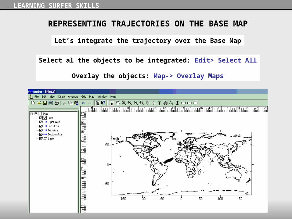
Let’s integrate the trajectory over the Base Map
Select al the objects to be integrated: Edit> Select All
Overlay the objects: Map-> Overlay Maps

REPRESENTING TRAJECTORIES ON THE BASE MAP
LEARNING SURFER SKILLS
Select the Post Map in the left column and improve the trajectory (red points, 0.03 cm size)
Select the Limits option in the Post Map properties and make a zoom (Lon: 50ºW-0º, Lat: 0º-20ºN)
REPRESENTING TRAJECTORIES ON THE BASE MAP
LEARNING SURFER SKILLS
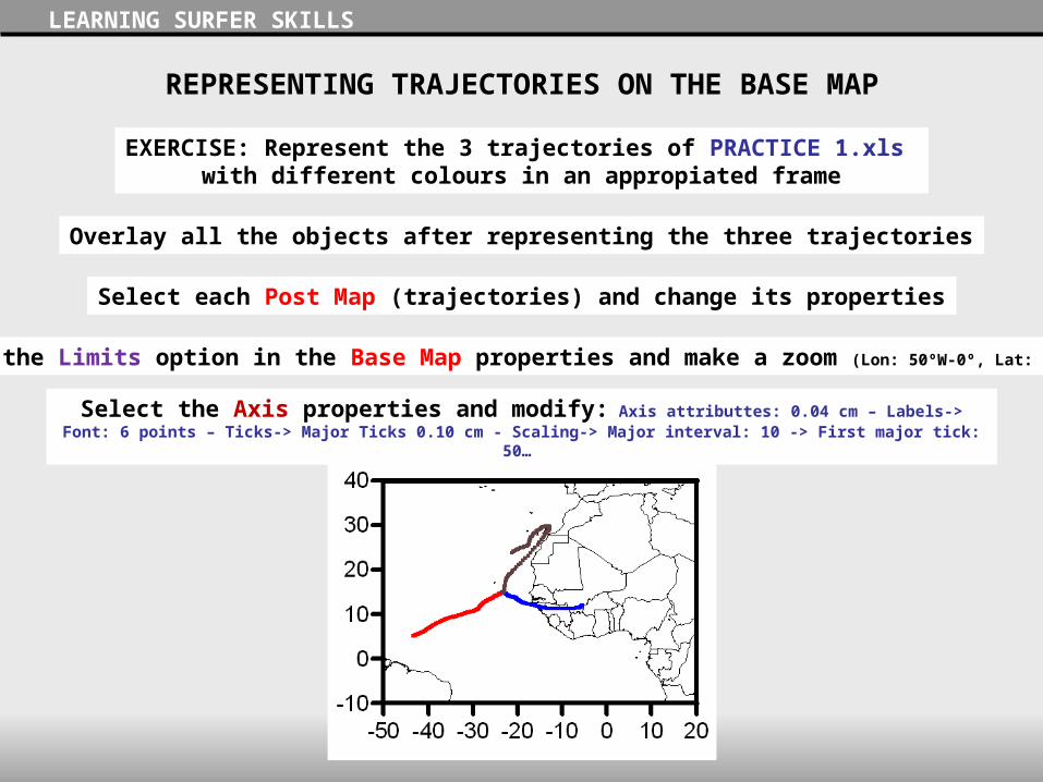
EXERCISE: Represent the 3 trajectories of PRACTICE 1.xls with different colours in an appropiated frame
Select the Limits option in the Base Map properties and make a zoom (Lon: 50ºW-0º, Lat: 10ºS-40ºN)
Overlay all the objects after representing the three trajectories
Select each Post Map (trajectories) and change its properties
Select the Axis properties and modify: Axis attributtes: 0.04 cm – Labels-> Font: 6 points – Ticks-> Major Ticks 0.10 cm - Scaling-> Major interval: 10 -> First major tick: 50…

REPRESENTING METEOROLOGICAL FIELDS ON THE BASE MAP
LEARNING SURFER SKILLS
• SURFER allows creating and representing a regularly spaced grid of variables
First of all it is necessary to create the grid file from an XYZ data file
We will use daily fields of meteorological variables (sea level pressure, 850 hPa geopotential height,…)
Go to: C:\course\Practice1\PRACTICE 1.xls
Worksheet “DAILY FIELDS” contains the dialy fields of geopotential height at the 850 hPa level for the 3 trajectories (13/Jul/2011, 24/Ene/2011 and 31/Jul/2011) at 12 UTC
Create the grid file: Grid-> Data
Select:• the columns of data XYZ
• the name of the output grid file
• the Kriging gridding method
REPRESENTING METEOROLOGICAL FIELDS ON THE BASE MAP
LEARNING SURFER SKILLS
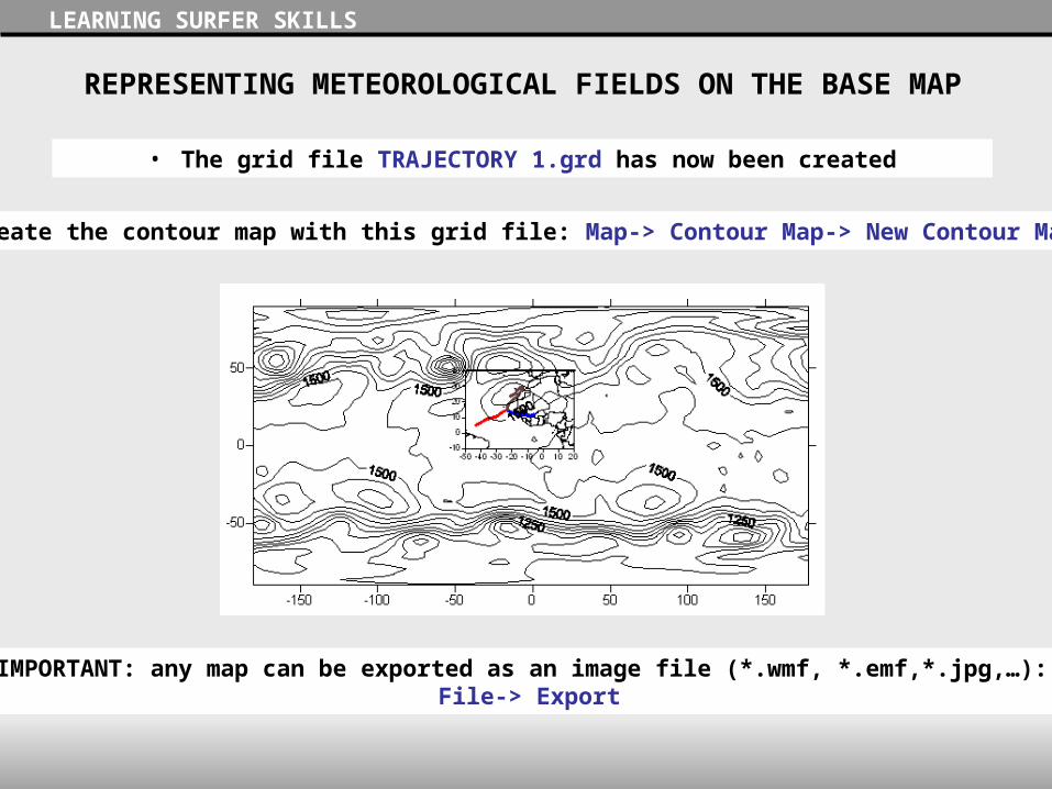
• The grid file TRAJECTORY 1.grd has now been created
Create the contour map with this grid file: Map-> Contour Map-> New Contour Map
IMPORTANT: any map can be exported as an image file (*.wmf, *.emf,*.jpg,…): File-> Export
REPRESENTING METEOROLOGICAL FIELDS ON THE BASE MAP
LEARNING SURFER SKILLS
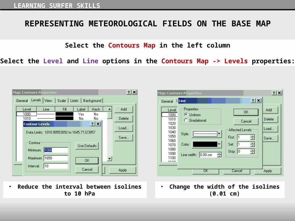
Select the Contours Map in the left column
Select the Level and Line options in the Contours Map -> Levels properties:
• Reduce the interval between isolines to 10 hPa • Change the width of the isolines (0.01 cm)
REPRESENTING METEOROLOGICAL FIELDS ON THE BASE MAP
LEARNING SURFER SKILLS
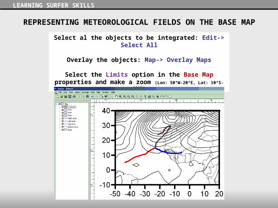
Select al the objects to be integrated: Edit-> Select All
Overlay the objects: Map-> Overlay Maps
Select the Limits option in the Base Map properties and make a zoom (Lon: 50ºW-20ºE, Lat: 10ºS-40ºN)
REPRESENTING METEOROLOGICAL FIELDS ON THE BASE MAP
LEARNING SURFER SKILLS
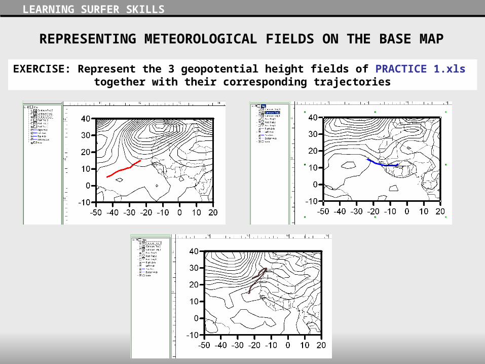
EXERCISE: Represent the 3 geopotential height fields of PRACTICE 1.xls together with their corresponding trajectories
CLUSTER ANALYSIS
2- CLUSTER ANALYSIS: CAPE VERDE, A CASE STUDY
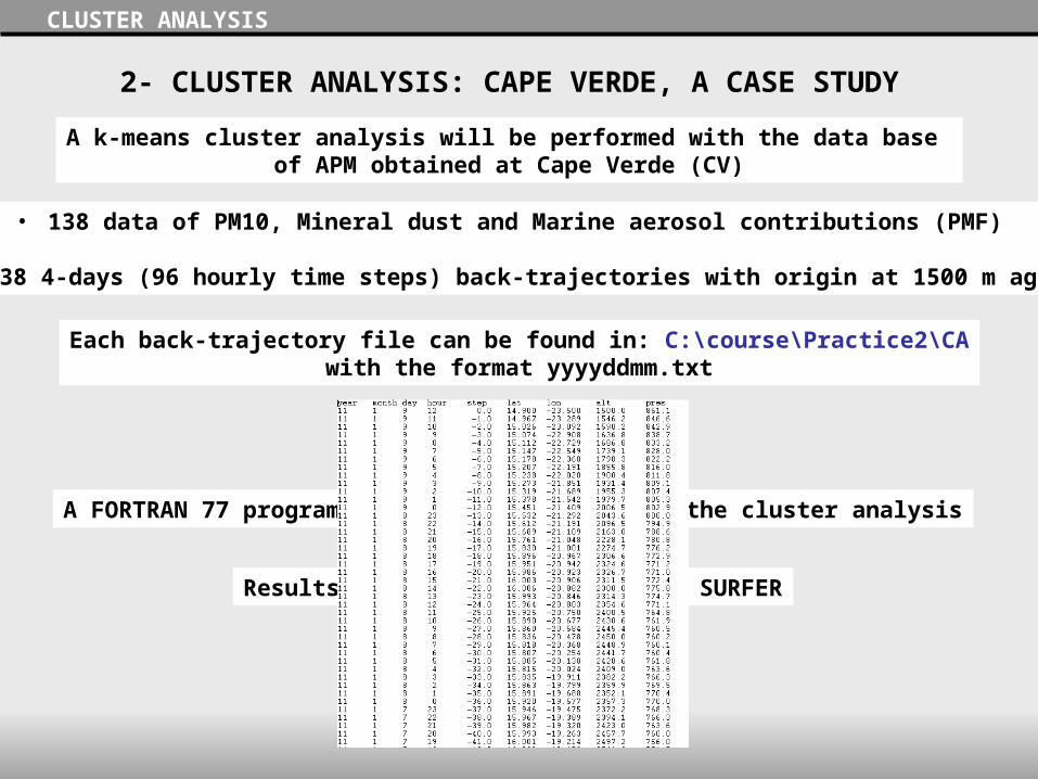
A k-means cluster analysis will be performed with the data base of APM obtained at Cape Verde (CV)
• 138 data of PM10, Mineral dust and Marine aerosol contributions (PMF)
• 138 4-days (96 hourly time steps) back-trajectories with origin at 1500 m agl
A FORTRAN 77 program will be used to perform the cluster analysis
Results will be represented with SURFER
Each back-trajectory file can be found in: C:\course\Practice2\CAwith the format yyyyddmm.txt

CLUSTER ANALYSIS
2- CLUSTER ANALYSIS: CAPE VERDE, A CASE STUDY
Open program: Compact Visual Fortran 6 -> Developer Studio
Open Workspace: File-> Open Workspace->C:\course\Practice2\CA\CA.dsw
The “DATES.txt” file contains the Dates of the trajectories with the format:
yyyymmdd
The “FIRST_CCENTERS.txt” file contains the Time steps of the initial cluster centers

CLUSTER ANALYSIS
2- CLUSTER ANALYSIS: CAPE VERDE, A CASE STUDY
Firstly, a 2-means CA will be performed for Cape Verde trajectories
2 trajectories with a different behaviour were selected by visual inspection
They are the 2 first trajectories of PRACTICE 1
CLUSTER ANALYSIS
2- CLUSTER ANALYSIS: CAPE VERDE, A CASE STUDY
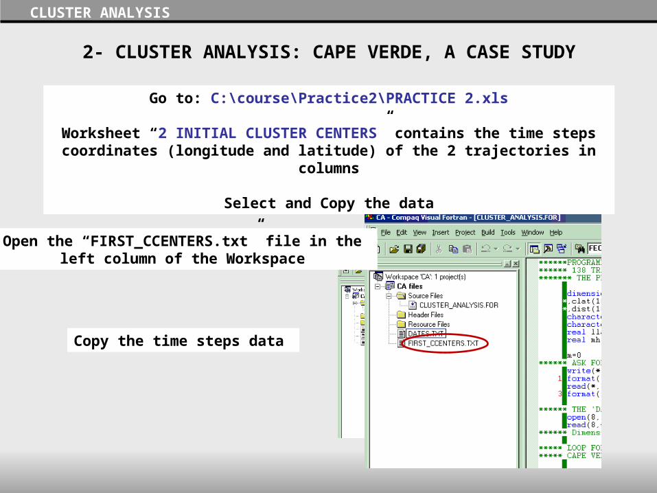
Go to: C:\course\Practice2\PRACTICE 2.xls
Worksheet “2 INITIAL CLUSTER CENTERS” contains the time steps coordinates (longitude and latitude) of the 2 trajectories in columns
Select and Copy the data
Open the “FIRST_CCENTERS.txt” file in the left column of the Workspace
Copy the time steps data
CLUSTER ANALYSIS
2- CLUSTER ANALYSIS: CAPE VERDE, A CASE STUDY
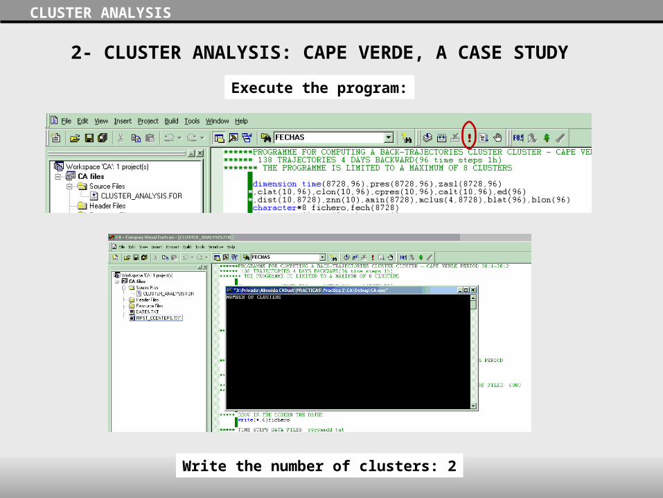
Execute the program:
Write the number of clusters: 2
CLUSTER ANALYSIS
2- CLUSTER ANALYSIS: CAPE VERDE, A CASE STUDY
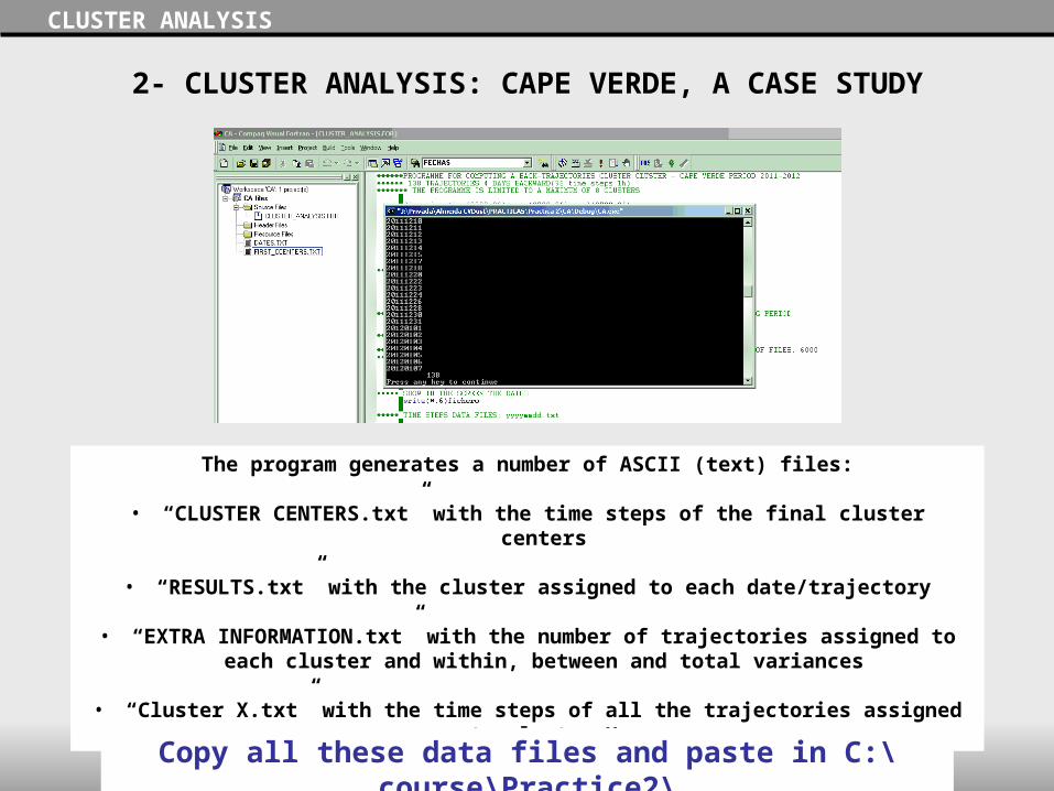
The program generates a number of ASCII (text) files:
• “CLUSTER CENTERS.txt” with the time steps of the final cluster centers
• “RESULTS.txt” with the cluster assigned to each date/trajectory
• “EXTRA INFORMATION.txt” with the number of trajectories assigned to each cluster and within, between and total variances
• “Cluster X.txt” with the time steps of all the trajectories assigned to cluster X
Copy all these data files and paste in C:\course\Practice2\

CLUSTER ANALYSIS
Open the SURFER program and load the Base map: Map-> Base MapGo to: C:\course\Practice2\World_BM.bln
Represent the cluster centers as Post Maps: Map> Post Map-> New Post MapGo to: C:\course\Practice2\CLUSTER CENTERS.txt
2- CLUSTER ANALYSIS: CAPE VERDE, A CASE STUDY
CLUSTER ANALYSIS
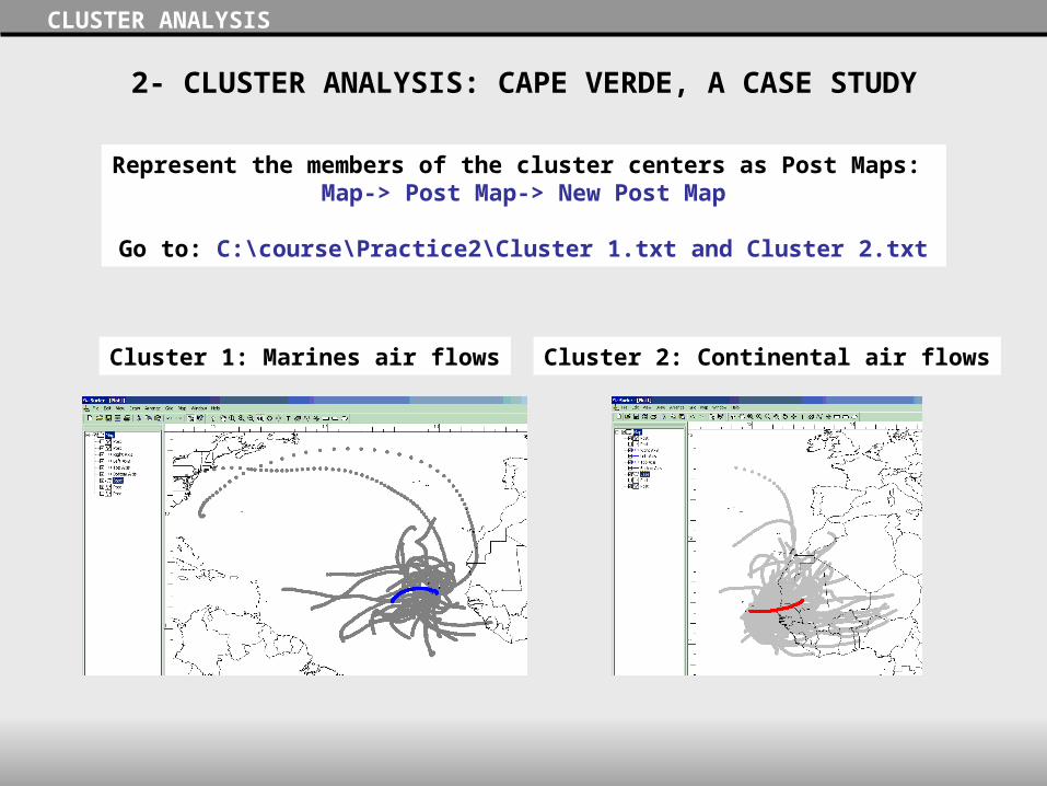
Represent the members of the cluster centers as Post Maps: Map-> Post Map-> New Post Map
Go to: C:\course\Practice2\Cluster 1.txt and Cluster 2.txt
Cluster 1: Marines air flows Cluster 2: Continental air flows
2- CLUSTER ANALYSIS: CAPE VERDE, A CASE STUDY
CLUSTER ANALYSIS
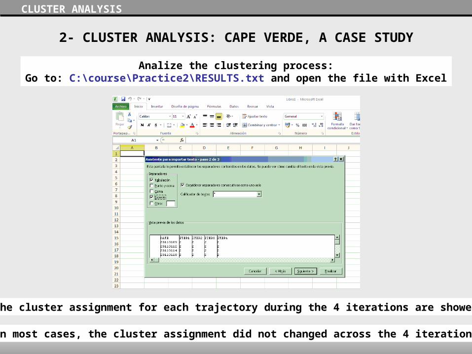
Analize the clustering process:Go to: C:\course\Practice2\RESULTS.txt and open the file with Excel
The cluster assignment for each trajectory during the 4 iterations are showed
In most cases, the cluster assignment did not changed across the 4 iterations
2- CLUSTER ANALYSIS: CAPE VERDE, A CASE STUDY
CLUSTER ANALYSIS
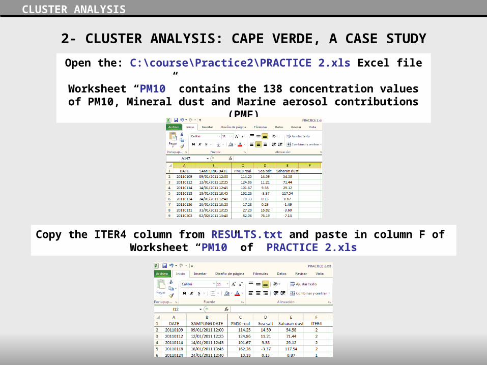
Open the: C:\course\Practice2\PRACTICE 2.xls Excel file
Worksheet “PM10” contains the 138 concentration values of PM10, Mineral dust and Marine aerosol contributions (PMF)
Copy the ITER4 column from RESULTS.txt and paste in column F of Worksheet “PM10” of PRACTICE 2.xls
2- CLUSTER ANALYSIS: CAPE VERDE, A CASE STUDY
CLUSTER ANALYSIS
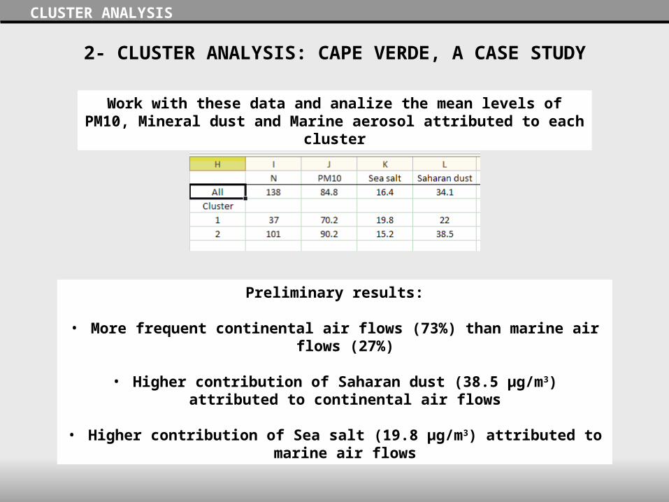
Work with these data and analize the mean levels of PM10, Mineral dust and Marine aerosol attributed to each cluster
Preliminary results:
• More frequent continental air flows (73%) than marine air flows (27%)
• Higher contribution of Saharan dust (38.5 µg/m3) attributed to continental air flows
• Higher contribution of Sea salt (19.8 µg/m3) attributed to marine air flows
2- CLUSTER ANALYSIS: CAPE VERDE, A CASE STUDY

CLUSTER ANALYSIS
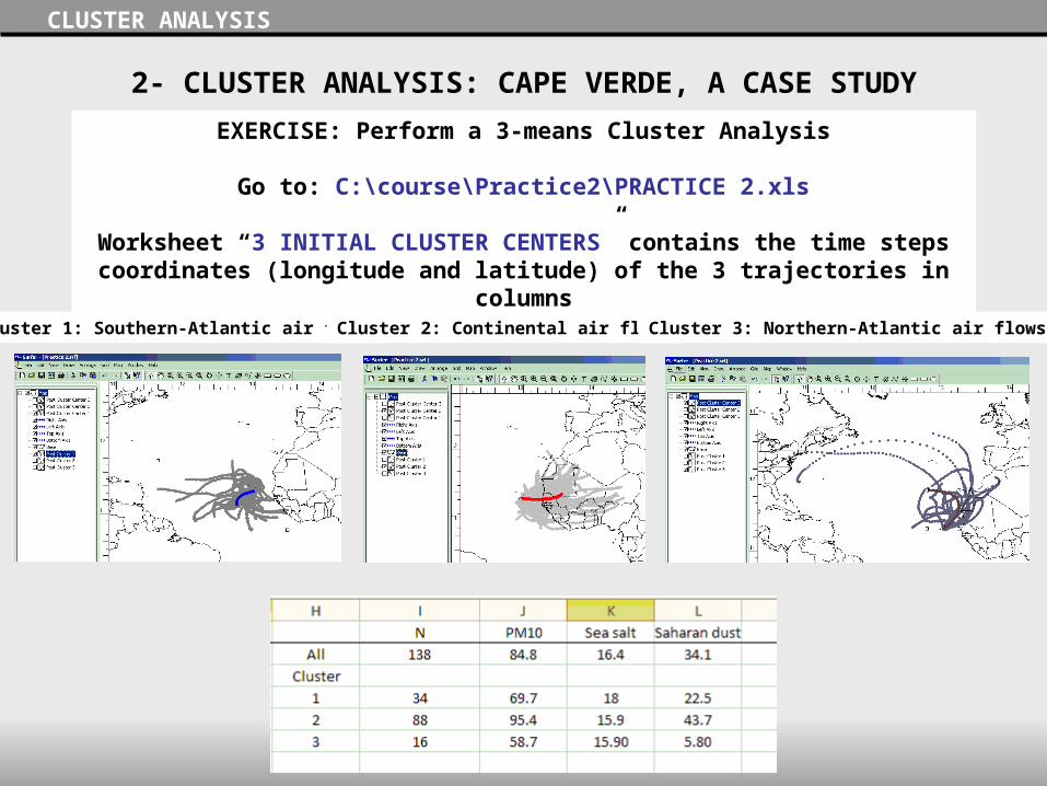
EXERCISE: Perform a 3-means Cluster Analysis
Go to: C:\course\Practice2\PRACTICE 2.xls
Page “3 INITIAL CLUSTER CENTERS” contains the time steps coordinates (longitude and latitude) of the 3 trajectories in columns
2- CLUSTER ANALYSIS: CAPE VERDE, A CASE STUDY
CLUSTER ANALYSIS
EXERCISE: Perform a 3-means Cluster Analysis
Go to: C:\course\Practice2\PRACTICE 2.xls
Worksheet “3 INITIAL CLUSTER CENTERS” contains the time steps coordinates (longitude and latitude) of the 3 trajectories in columns
Cluster 1: Southern-Atlantic air flows Cluster 2: Continental air flows Cluster 3: Northern-Atlantic air flows
2- CLUSTER ANALYSIS: CAPE VERDE, A CASE STUDY
3 – RESIDENCE TIME ANALYSIS: CAPE VERDE, A CASE STUDY
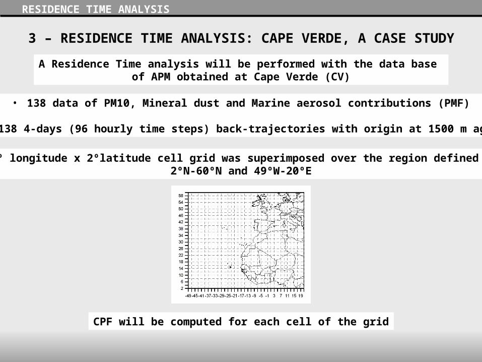
A Residence Time analysis will be performed with the data base of APM obtained at Cape Verde (CV)
• 138 data of PM10, Mineral dust and Marine aerosol contributions (PMF)
• 138 4-days (96 hourly time steps) back-trajectories with origin at 1500 m agl
CPF will be computed for each cell of the grid
A 2º longitude x 2ºlatitude cell grid was superimposed over the region defined by 2ºN-60ºN and 49ºW-20ºE
RESIDENCE TIME ANALYSIS
3 – RESIDENCE TIME ANALYSIS: CAPE VERDE, A CASE STUDY
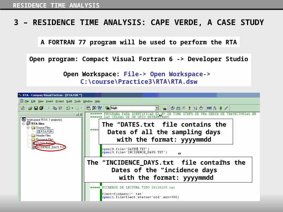
A FORTRAN 77 program will be used to perform the RTA
RESIDENCE TIME ANALYSIS
Open program: Compact Visual Fortran 6 -> Developer Studio
Open Workspace: File-> Open Workspace-> C:\course\Practice3\RTA\RTA.dsw
The “INCIDENCE_DAYS.txt” file contains the Dates of the “incidence days”
with the format: yyyymmdd
The “DATES.txt” file contains the Dates of all the sampling days
with the format: yyyymmdd
3 – RESIDENCE TIME ANALYSIS: CAPE VERDE, A CASE STUDY
RESIDENCE TIME ANALYSIS
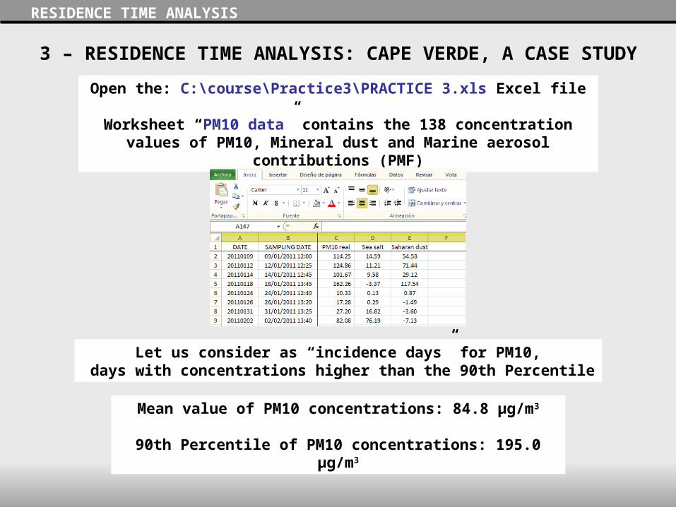
Open the: C:\course\Practice3\PRACTICE 3.xls Excel file
Worksheet “PM10 data” contains the 138 concentration values of PM10, Mineral dust and Marine aerosol contributions (PMF)
Let us consider as “incidence days” for PM10, days with concentrations higher than the 90th Percentile
Mean value of PM10 concentrations: 84.8 µg/m3
90th Percentile of PM10 concentrations: 195.0 µg/m3

3 – RESIDENCE TIME ANALYSIS: CAPE VERDE, A CASE STUDY
RESIDENCE TIME ANALYSIS
• Copy apart the DATE and PM10 columns
• Re-order the data from the highest to the lowest value of PM10 concentrations
• Select the dates of the incidence days:PM10 concentrations > 195.0 µg/m3
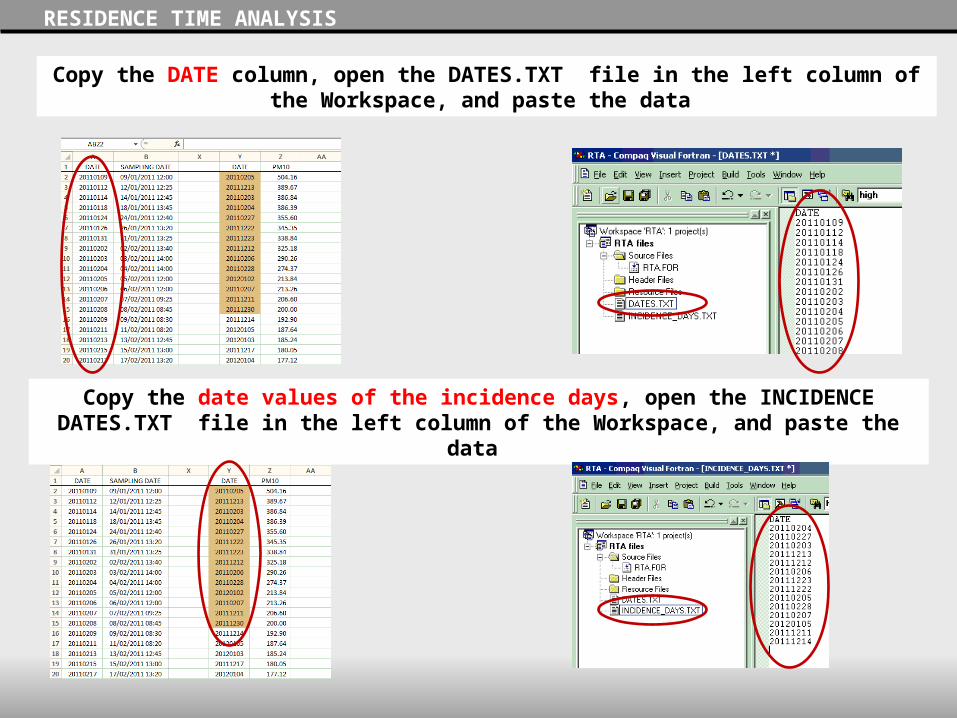
Copy the DATE column, open the DATES.TXT file in the left column of the Workspace, and paste the data
RESIDENCE TIME ANALYSIS
Copy the date values of the incidence days, open the INCIDENCE DATES.TXT file in the left column of the Workspace, and paste the data
RESIDENCE TIME ANALYSIS
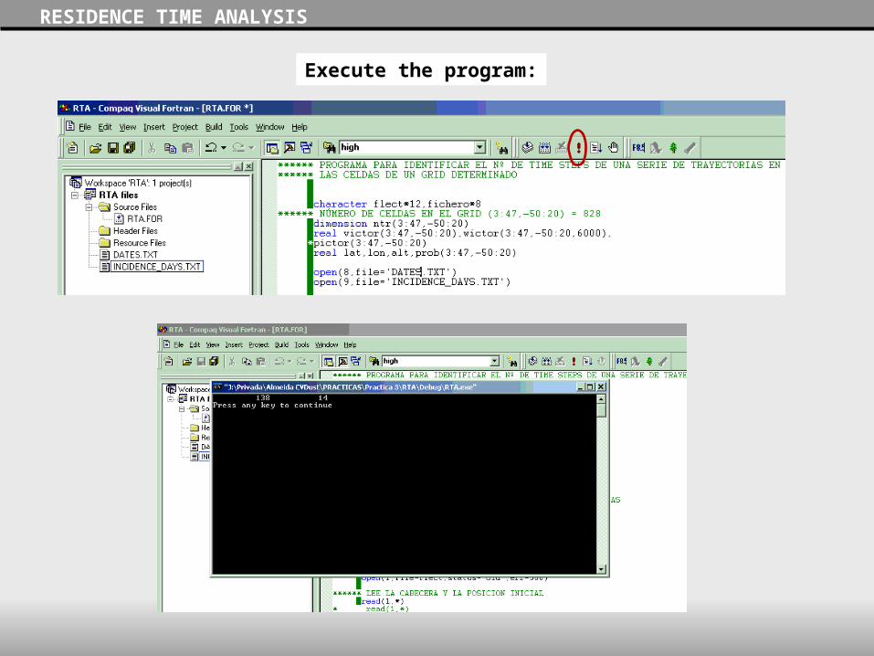
Execute the program:

RESIDENCE TIME ANALYSIS
This program reads each back-trajectory file (in: C:\course\Practice3\RTA)with the format yyyyddmm.txt, for all the sampling dates (DATES.txt) and
the Incidence days dates (INCIDENCE_DAYS.txt)
• The number of time-steps residing on each grid cell is calculated for all the sampling dates (TS) and for the Incidence days dates (ID)
• The number of trajectories contributing with time steps to each grid cell is calculated (Ntr)
• For each grid cell with >1 time step-> CPF=(ID)/(TS)
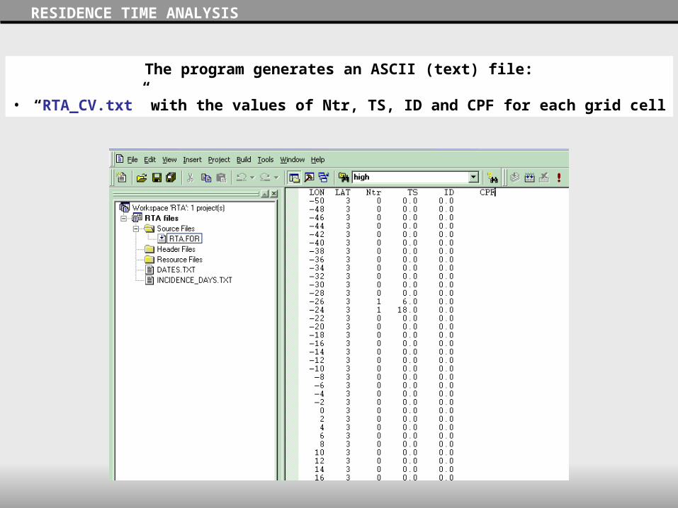
The program generates an ASCII (text) file:
• “RTA_CV.txt” with the values of Ntr, TS, ID and CPF for each grid cell
RESIDENCE TIME ANALYSIS

RESIDENCE TIME ANALYSIS
Go to: C:\course\Practice3\RTA\RTA_CV.txt and open the file with Excel
Copy the 5 columns and paste in the C:\course\Practice3\PRACTICE 3.xls Excel file in a new worksheet called “RTA”

RESIDENCE TIME ANALYSIS
Copy the column B from worksheet “9 PF” of PRACTICE 3.xls and paste in column G (next to the CPF values) of worksheet “RTA”
A 9 point filter is thus computed to smooth the CPF map and preserve significant variations

RESIDENCE TIME ANALYSIS
REPRESENTING THE CPF MAP
Open the SURFER program and load the Base map: Map-> Base MapGo to: C:\course\Practice3\World_BM.bln
Represent the CPF as a Classed Post Map: Map> Post Map-> New Classed Post Map
Go to: C:\course\Practice3\PRACTICE 3.xls and pick: RTA worksheet
Select the 9 POINT FILTER column as the Z variable
in the General options
Select the Classed Post in the left column where all the objects of your map are displayed
Select the Classes options :5 classes
Binning Method: Equal intervalsSymbol: squareSyze: 0.08 cm

RESIDENCE TIME ANALYSIS
REPRESENTING THE CPF MAP
Select al the objects to be integrated: Edit> Select All
Overlay the objects: Map-> Overlay Maps
REPRESENTING THE CPF MAP
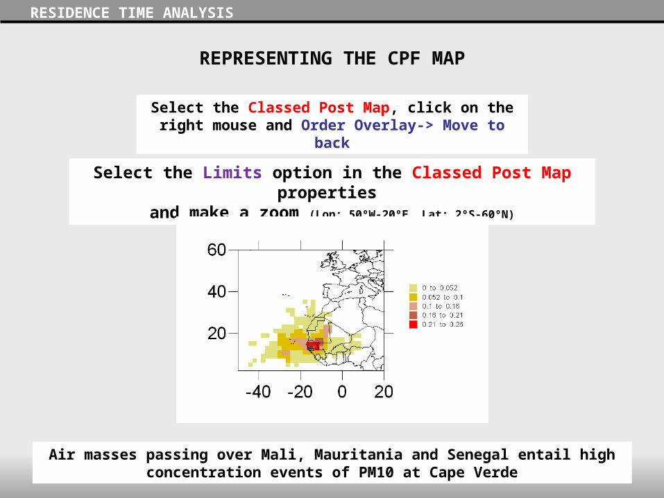
Select the Classed Post Map, click on the right mouse and Order Overlay-> Move to back
RESIDENCE TIME ANALYSIS
Select the Limits option in the Classed Post Map properties and make a zoom (Lon: 50ºW-20ºE, Lat: 2ºS-60ºN)
Air masses passing over Mali, Mauritania and Senegal entail high concentration events of PM10 at Cape Verde
REPRESENTING THE CPF MAP
RESIDENCE TIME ANALYSIS
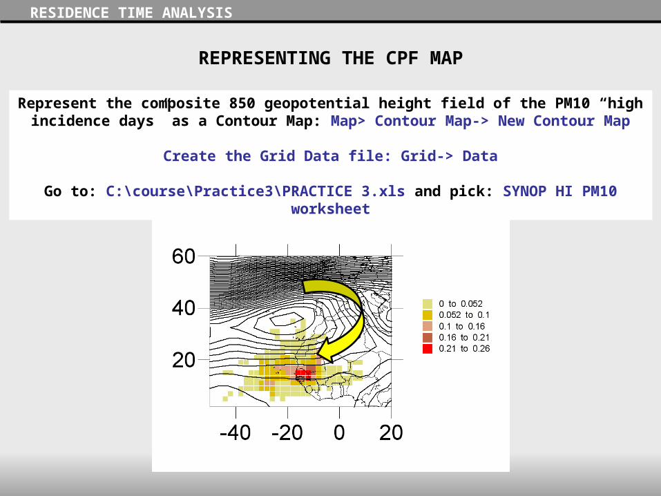
Represent the composite 850 geopotential height field of the PM10 “high incidence days” as a Contour Map: Map> Contour Map-> New Contour Map
Create the Grid Data file: Grid-> Data
Go to: C:\course\Practice3\PRACTICE 3.xls and pick: SYNOP HI PM10 worksheet

RESIDENCE TIME ANALYSIS
EXERCISE: Perform a RTA with “low incident days” for PM10
Go to: C:\course\Practice3\PRACTICE 3.xls
Worksheet “PM10 data” contains the 138 concentration values of PM10
Let us consider as “incidence days” for PM10, days with concentrations lower than the 10th Percentile
Mean value of PM10 concentrations: 84.8 µg/m3
10th Percentile of PM10 concentrations: 23.6 µg/m3

RESIDENCE TIME ANALYSIS
Air masses passing over south to southwestern atlantic areas entail low concentration events of PM10 at Cape Verde

ACKNOWLEDGEMENTS
ACKNOWLEDGEMENTS
THANK YOU VERY MUCH FOR YOUR ATTENTION