Applications of Tensor DecompositionsREU Site: Interdisciplinary Program in High Performance Computing

Sergio Garcia Tapia1, Rebecca Hsu2, Alyssa Hu3, Darren Stevens II4,Graduate assistant: Jonathan S. Graf5, Faculty mentor: Matthias K. Gobbert5, and

Client: Tyler Simon6

1Department of Mathematics, University at Buffalo, SUNY2Department of Mathematics, University of Maryland, College Park,3Department of Mathematics and Department of Computer Science,

University of Maryland, College Park4Department of Computer Science and Electrical Engineering, UMBC

5Department of Mathematics and Statistics, UMBC,6Laboratory for Physical Sciences

Technical Report HPCF–2016–17, hpcf.umbc.edu > Publications

Abstract

This report explores how data structures known as tensors can be used to performmultidimensional data analysis. If a matrix can be thought of as a two-dimensionalarray, then a tensor can be thought of as a multi-dimensional array (with more thantwo dimensions). Tensor decompositions are algorithms and tools that can allow theuser to directly perform analysis on this type of data. After explaining the basics oftensors, we work with two different three-dimensional data sets and decompose thetensors in order to provide analysis and interpretations of various aspects of the data.

Key words. Tensors, Tucker tensors, Principal component analysis.

1 Introduction

Many application problems in data analysis inherently contain multi-dimensional data. Po-tential examples can include behavioral studies across different situations, facial recognitionalgorithms, and signals processing and analysis. Matrices are oftentimes used to organizethe variables reorded after having found an appropriate way to express the data in the two-dimensional array. On the other hand, one can also directly perform analysis on the data byusing multi-dimensional arrays that preserve the inherent structure of such multi-dimensionaldata represented by tensors.

The basics of how to use and operate with tensors are similar to operations with regulartwo-dimensional matrices. With third-order (three-dimensional) tensors, it is clearer tovisualize them as slices of matrices overlayed on top of each other. Multiplying tensorsrequires an extra step; one must unfold the tensor into a matrix before proceeding withtraditional matrix multiplication and then refold the result back into a higher order tensor.For multi-dimensional data, one would normally perform dimension reduction techniquesto organize the data into a matrix. Then, a method such as principal component analysis

1

(PCA) would be applied on the matrix in order to provide analysis of the data. However,we can apply what is known as a tensor decomposition to all of the multi-dimensional dataat once. One specific tensor decomposition for N -dimensional tensors is called the Tuckerdecomposition [6]; specifically for 3-dimensional data, Kiers et al. [4] also refer to it as 3-mode-PCA (3MPCA). This decomposition factors the original data into a core tensor thatis typically smaller, as well as three factor matrices that measure the level of interactionbetween the data [6]. Section 2 introduces some basic facts and properties of tensors andexplains the Tucker decomposition more in-depth.

The Matlab Tensor Toolbox1 has many functions available for creating and operatingwith tensors, some of which we will discuss in Section 3. The Tensor Toolbox can be usedto create sparse or regular tensors. Sparse tensors are tensors for which most of the entriesare zero. If most of the elements of a tensor are nonzero, the tensor is considered regularor dense. In addition, there are commands to multiply tensors with other tensors and withother vectors or matrices. There are in fact functions for working with tensors that havespecific properties, as well as relevant decompositions, such as Tucker or Kruskal tensors.Section 3 discusses the features of the Matlab Tensor Toolbox in more detail.

In order to provide an illustrative example, Kiers [4] provides a fictitious set of dataas a behavioral study for six different individuals measuring five behavioral responses infour different scenarios. This data is naturally multi-dimensional and can be expressed asa 6 × 5 × 4 tensor. Kiers applies the 3MPCA decomposition to this data to generate thecomponent matrices and desired core tensor. Labels were given to each of the componentsafter seeing the column groupings in order to provide a clear interpretation of the data.Kiers demonstrates mathematically how to use the results of the decomposition in order toretrieve the original data. This is shown in detail in Section 4.

Section 5 introduces data from a Dutch psychological experiment with a 326 × 5 × 2tensor. We apply the Tucker decomposition also to this data set and then use additionalsteps to use the result. Kiers used the component matrices’ columns to group data andgenerated labels for those columns. For the Dutch data set, we take the dot product of theoriginal data with the column(s) of the component matrix B to better summarize the data.We note how we can input different core tensor sizes and if that affects resulting componentmatrices and interpretation.

2 Tensor Analysis

2.1 Tensor Basics

We now formally introduce tensors. Material presented here is based on the Kolda and Baderpaper [6]. Recall that a matrix U ∈ RI×J can be thought of as a 2-dimensional array, whereI, J are positive integers. A tensor X ∈ RI1×...×IN is a generalization of a matrix; that is, it isan N -dimensional array. As such, many properties and operations of matrices are retainedin higher dimensions with some concepts being more intricate. Tensors are denoted by Euler

1Version 2.6, http://www.sandia.gov/~tgkolda/TensorToolbox/index-2.6.html

2

Figure 2.1: A tensor of order 3.

script characters as first done above in the usage of X. An element in a tensor is denotedby xi1,...,iN , where in = 1, . . . , In (that is, the subscripts range from 1 to their correspondinguppercase equivalent). An N -dimensional tensor is also referred to sometimes as a tensorof order N , or a tensor with N modes. Addition is done element-wise as one would expect,and the Frobenius norm of a tensor is the same as that of a matrix, satisfying

||X|| =

√√√√ I1∑i1=1

· · ·IN∑

iN=1

x2i1,...,iN

for X ∈ RI1×...×IN .

For N -way tensor X, fibers and slices are defined by fixing N − 1 and N − 2 indices,respectively. The fibers then are 1-dimensional tensors or arrays (vectors), and the slices are2-dimensional tensors or arrays (matrix) obtained from X with some orientation that dependson what indices have been fixed. For illustrative purposes, we limit our discussion to 3-waytensors and provide Figure 2.1 as a way to visualize them. For a tensor X ∈ RI×J×K of 3dimensions, on the one hand, a fiber is obtained by fixing two of the indices. The possiblechoices then are vectors X(:, j, k), X(i, :, k), and X(i, j, :), for i = 1, . . . , I, j = 1, . . . , J ,and k = 1, . . . , K; these correspond to columns, rows, and tube fibers, respectively. InFigure 2.2, we see that fibers of a 3-way tensor are pillars with some orientation. On theother hand, a slice of a tensor X is obtained by fixing one of the indices and the choiceswould be matrices X(i, :, :), X(:, j, :), and X(:, :, k) that correspond to horizontal, lateral, andfrontal slices, respectively. In Figure 2.3, we see that the the slices of a 3-way tensor arerepresented as planes with certain orientations.

Introducing fibers also allows us to introduce the idea of unfolding tensors. Visually, themode-n unfolding or matricization of a 3-way tensor G ∈ RP×Q×R, where n = 1, 2, or 3,means to take the mode-n fibers, to rotate them into column orientation, and then line themup sequentially. The result is that we express a tensor G as a matrix G(n) with dimensionsthat depend on n = 1, 2, 3, as well as P,Q,R. The benefit of this is that it allows us toconsider mode-n matrix multiplication. The mode-n product between a tensor and matrixis defined if certain dimensions match as is the case for matrices. If G ∈ RP×Q×R is a tensor

3

Figure 2.2: Fiber representations of a 3-way tensor.

Figure 2.3: Slice representations of a 3-way tensor.

of 3 modes, and if G(3) ∈ RR×PQ is its mode-3 unfolding, then the mode-3 product with amatrix C ∈ RK×R is expressed as

Y = G×3 C ⇐⇒ Y(3) = CG(3).

where Y ∈ RP×Q×K , and Y(3) ∈ RK×PQ is its mode-3 unfolding. An example of this isexplored in detail in Section 4.

2.2 Principal Component Analysis

In spite of tensors having the ability to inherently represent multi-dimensional data, it iscommonplace for matrices to be preferred. As a result, many methods for dealing withmulti-dimensional data by using matrices have been developed. Among them is principalcomponent analysis (PCA), a technique that seeks to find an appropriate representation fordata that has been collected and organized in a matrix. Generally, data is arranged in amatrix U such that each column constitutes a different type of measurement performed andeach row a different trial. The goal is then to find a matrix P such that its vectors (known asthe principal components of U) are a basis for the row space of U where the trial vectors arecontained. Since each principal vector is associated with a corresponding variance betweenmeasurement types in A, the independent directions related to a large variance suggestunderlying patterns in the data. A generalization of this technique to higher-order tensorshas been developed and it is known as a Tucker decomposition [6] or 3MPCA [4]. Theconvenience is that we are then able to retain the multi-dimensional nature of data andperform analysis on thit directly, instead of having to represent it as a matrix to use matrixanalysis techniques.

4

Figure 2.4: Visual representation of Tucker decomposition.

2.3 Tucker Tensor Decomposition

We mentioned that tensors can be decomposed. Here, we concern ourselves with a methodresembling PCA, known as the Tucker decomposition. Given a tensor X ∈ RI×J×K , a Tuckerdecomposition attempts to express it as

X ≈ G×1 A×2 B ×3 C (2.1)

for core tensor G ∈ RP×Q×R, and with A ∈ RI×P , B ∈ RJ×Q, and C ∈ RK×R being factormatrices that are orthogonal visually represented by Figure 2.4, for integers 1 ≤ P ≤ I,1 ≤ Q ≤ J , and 1 ≤ R ≤ K. The numbered subscripts indicate the mode of multiplicationin which the product between the tensor G and the matrices are being multiplied that wasdiscussed in Section 2.1. The entries themselves are given by

xijk ≈P∑

p=1

Q∑q=1

R∑r=1

gpqraipbjqckr.

By saying the decomposition resembles PCA, we mean that it is a form of higher-orderprincipal component analysis where the component matrices are principal components [6],which is why Kiers [4] refers to it as 3MPCA. Therefore, we oftentimes use 3MPCA andTucker decomposition interchangeably. The way in which to interpret the components of thedecomposition is also sometimes dependent on the data set in question. Since the componentmatrices measure the level of interaction [6] between the information recorded, the techniquecan be used to group several variables that are most closely related to one another, as wedemonstrate in Section 4. Alternatively, the decomposed result can be used jointly with theoriginal data to provide insight into the recorded information, as shown in Section 5.

The Tucker decomposition for a given tensor is defined for different core tensor sizes, andtherefore the decomposition is not unique. The decomposition can be computed throughnumerical methods such as Alternating Least Squares (ALS), which is an iterative methodthat depends on an initial guess, a stopping tolerance, and more, thus the result is not uniqueeven for one choice of core tensor size.

5

3 Matlab Tensor Toolbox

The Tensor Toolbox has many functions available for creating and operating with tensorsin Matlab. In particular, there are specific functions for working with tensors of specificstructures, including regular tensors, sparse tensors, and Tucker-decomposed tensors.

3.1 Literature Review

The Tensor Toolbox for Matlab has been used and referenced in different research papers.Kolda and Bader’s paper on Tensor Decompositions and Applications served as backgroundreading for our research [6]. Other papers with interesting applications of the Tensor Toolboxwill be briefly discussed. Fitzgerald, Coyle, and Cranitch investigate the separation of drumsounds from music with tensor factorization models [2]. Also, a lot of data can be representedwith links and graphs, especially those involving relationships such as online connections insocial networks. Thus, the Tensor Toolbox can be applied to predict future links, specificallyby using a CP tensor decomposition (involving Alternating Least Squares) [1]. The TensorToolbox is compared to GigaTensor, an algorithm used to deal with large tensors and theirdecompositions, using Hadoop MapReduce [3]. Tensor Toolbox runs faster than GigaTensorwhen the size of the tensor (with same-size modes) is less than 107. However, any tensor ofsize greater than 107 and the Tensor Toolbox runs out of memory; thus, GigaTensor is helpfulto use, as it appears to support tensors at least of size 109 [8]. Furthermore, Kolda and Sunpreviously commented on memory issues of applying Tucker on a large sparse tensor in a2008 paper and propose a Memory Efficient Tucker method to avoid memory overflow [5].

3.2 Regular (Dense) Tensors

The tensor command is the most basic, which converts an existing array A into a tensor.Additionally, the user is allowed to pass an array argument specifying the desired size (e.g.,[2 3 4] for a 2 × 3 × 4 tensor). Alternatively, one can use the tenrand function to createa random tensor of a size determined by the passed array argument. Similar to functionsones and zeroes for matrices, the functions tenones and tenzeros create tensors of adesired size filled with ones and zeros, respectively. Having created a tensor, a user mightbe interested in information about it, such as its size or the information stored in it. Suchinquiry can be done for a tensor X by X.size and X.data (or double(X)), with the formerreturning an array with the size and the latter a multi-dimensional array with the data thatthe tensor contains. In fact, using these two in conjunction is an easy way to replicate thetensor by passing the data array and size array. The extraction of elements is the same asfor matrices, since one can just pass specific indices (or array of indices). Lastly, component-wise operations can be done with the dot operator, such as X.*Y for multiplication, or X./Yfor division. Some functions, like the sqrt function for matrices, cannot be used; instead,the tenfun(@foo, X) is needed to perform the component-wise operations defined in somecustom @foo function (note the character preceding the function name) to an existing tensorX. For instance, tenfun(@sqrt,X) takes the square root of every element in X.

6

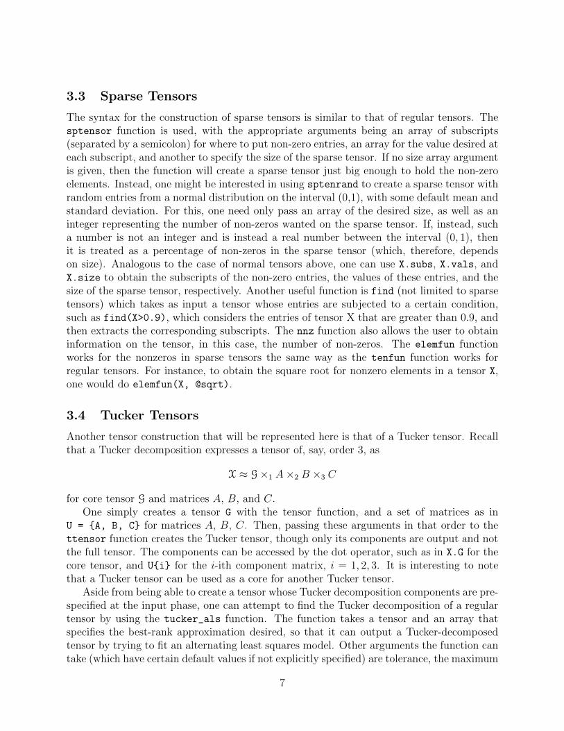
3.3 Sparse Tensors

The syntax for the construction of sparse tensors is similar to that of regular tensors. Thesptensor function is used, with the appropriate arguments being an array of subscripts(separated by a semicolon) for where to put non-zero entries, an array for the value desired ateach subscript, and another to specify the size of the sparse tensor. If no size array argumentis given, then the function will create a sparse tensor just big enough to hold the non-zeroelements. Instead, one might be interested in using sptenrand to create a sparse tensor withrandom entries from a normal distribution on the interval (0,1), with some default mean andstandard deviation. For this, one need only pass an array of the desired size, as well as aninteger representing the number of non-zeros wanted on the sparse tensor. If, instead, sucha number is not an integer and is instead a real number between the interval (0, 1), thenit is treated as a percentage of non-zeros in the sparse tensor (which, therefore, dependson size). Analogous to the case of normal tensors above, one can use X.subs, X.vals, andX.size to obtain the subscripts of the non-zero entries, the values of these entries, and thesize of the sparse tensor, respectively. Another useful function is find (not limited to sparsetensors) which takes as input a tensor whose entries are subjected to a certain condition,such as find(X>0.9), which considers the entries of tensor X that are greater than 0.9, andthen extracts the corresponding subscripts. The nnz function also allows the user to obtaininformation on the tensor, in this case, the number of non-zeros. The elemfun functionworks for the nonzeros in sparse tensors the same way as the tenfun function works forregular tensors. For instance, to obtain the square root for nonzero elements in a tensor X,one would do elemfun(X, @sqrt).

3.4 Tucker Tensors

Another tensor construction that will be represented here is that of a Tucker tensor. Recallthat a Tucker decomposition expresses a tensor of, say, order 3, as

X ≈ G×1 A×2 B ×3 C

for core tensor G and matrices A, B, and C.One simply creates a tensor G with the tensor function, and a set of matrices as in

U = {A, B, C} for matrices A, B, C. Then, passing these arguments in that order to thettensor function creates the Tucker tensor, though only its components are output and notthe full tensor. The components can be accessed by the dot operator, such as in X.G for thecore tensor, and U{i} for the i-ith component matrix, i = 1, 2, 3. It is interesting to notethat a Tucker tensor can be used as a core for another Tucker tensor.

Aside from being able to create a tensor whose Tucker decomposition components are pre-specified at the input phase, one can attempt to find the Tucker decomposition of a regulartensor by using the tucker_als function. The function takes a tensor and an array thatspecifies the best-rank approximation desired, so that it can output a Tucker-decomposedtensor by trying to fit an alternating least squares model. Other arguments the function cantake (which have certain default values if not explicitly specified) are tolerance, the maximum

7

number of iterations, and an initial guess. The idea is that if we know the rank Rn of thematrix obtained from each mode-n unfolding of the tensor and provide this as input, thenthe decomposition is more likely to be accurate.

3.5 Tensor Products and Miscellaneous

Tensor operations such as multiplication are handled with the ttv, ttm, and ttt. The firsttakes as arguments a tensor, a vector, and a number indicating the mode of multiplication (sothat the product is defined). One can pass multiple vectors at once if enclosed in curly braces,such as {A, B, C, D}, followed by an array specifying the mode in which the vectors willbe multiplied with the tensor. In the context above, it could be as [1 3], which suggeststhe multiplications that will take place are the tensor with A in mode-1 and with C inmode-3, with the other multiplications not carried out since they are unspecified. The ttm

multiplication works the same way. Lastly, the ttt function is used to multiply two tensors.One simply passes the two tensors as arguments and two arrays specifying which modes willbe multiplied with each other (the order matters, for this might be the difference betweenthe product being handled as an outer product or an inner product).

If at any point one wishes to unfold these tensors (that is, matricize them), one can doso with the tenmat function. Simply pass as arguments the tensor, X, and two arrays; onespecifying the modes to be converted to rows, and the other specifying the modes to beconverted to columns. Additionally, any type of tensor can be converted into a regular typeof tensor via the full command, which takes as input any type of tensor and returns a dense(regular) tensor.

4 Illustrative Example of Tensor Decomposition

As discussed, the purpose of utilizing tensors and their decompositions is to make analyzingmulti-dimensional data easier. Kiers et al. [4] provide several data sets that illustrate theTucker decomposition and their respective interpretations, and they provide one particularlysmall illustrative example, for which the multiplication of the Tucker decomposition can beexplicitly checked. Note that the article refers to this decomposition as 3MPCA and we willuse this term while referring to tables from this article.

4.1 Original Input Data

Table 4.1 shows the original fictitious data provided in the Kiers article that will be used forthe decomposition [4]. This table shows the scores of

• I = 6 individuals — Anne, Bert, Claus, Dolly, Edna, and Frances — displaying

• J = 5 behavior types — emotional (E), sensitive (S), caring (C), thorough (T), andaccurate (A) — in

8

Table 4.1: Fictitious data set of scores of six individuals on five response variables for foursituations.

Doing an exam Giving a speech Family Picnic Meeting a new dateIndividual E S C T A E S C T A E S C T A E S C T AAnne 0.0 0.0 1.2 3.0 3.0 0.6 0.6 1.3 2.4 2.4 3.0 3.0 1.8 0.0 0.0 3.6 3.6 2.5 0.9 0.9Bert 0.0 0.0 0.8 2.0 2.0 0.2 0.2 0.8 1.8 1.8 1.0 1.0 1.0 1.0 1.0 1.2 1.2 1.4 1.8 1.8Claus 0.0 0.0 0.8 2.0 2.0 0.2 0.2 0.8 1.8 1.8 1.0 1.0 1.0 1.0 1.0 1.2 1.2 1.4 1.8 1.8Dolly 0.0 0.0 1.2 3.0 3.0 0.6 0.6 1.3 2.4 2.4 3.0 3.0 1.8 0.0 0.0 3.6 3.6 2.5 0.9 0.9Edna 0.0 0.0 1.0 2.5 2.5 0.4 0.4 1.1 2.1 2.1 2.0 2.0 1.4 0.5 0.5 2.4 2.4 2.0 1.3 1.3Frances 0.0 0.0 1.2 3.0 3.0 0.6 0.6 1.3 2.4 2.4 3.0 3.0 1.8 0.0 0.0 3.6 3.6 2.5 0.9 0.9

• K = 4 different situations — doing an exam, giving a speech, family picnic, andmeeting a new date.

The data is presented in Table 4.1 in the form of the original (fictitious) psychologicalexperiment. It gives naturally rise to a tensor of data X ∈ R6×5×4, where the matrix ofnumbers in each subtable of the four situations is one slice X(:, :, k) ∈ R6×5 for each k =1, . . . , 4, that is,

X(:, :, 1) =

0.0 0.0 1.2 3.0 3.00.0 0.0 0.8 2.0 2.00.0 0.0 0.8 2.0 2.00.0 0.0 1.2 3.0 3.00.0 0.0 1.0 2.5 2.50.0 0.0 1.2 3.0 3.0

, X(:, :, 2) =

0.6 0.6 1.3 2.4 2.40.2 0.2 0.8 1.8 1.80.2 0.2 0.8 1.8 1.80.6 0.6 1.3 2.4 2.40.4 0.4 1.1 2.1 2.10.6 0.6 1.3 2.4 2.4

,

X(:, :, 3) =

3.0 3.0 1.8 0.0 0.01.0 1.0 1.0 1.0 1.01.0 1.0 1.0 1.0 1.03.0 3.0 1.8 0.0 0.02.0 2.0 1.4 0.5 0.53.0 3.0 1.8 0.0 0.0

, X(:, :, 4) =

3.6 3.6 2.5 0.9 0.91.2 1.2 1.4 1.8 1.81.2 1.2 1.4 1.8 1.83.6 3.6 2.5 0.9 0.92.4 2.4 2.0 1.3 1.33.6 3.6 2.5 0.9 0.9

.

4.2 Illustrative 3MPCA Decomposition

Now, recall that a Tucker decomposition of a 3-way tensor X expresses the tensor as in (2.1).Since we specify the size we want our core tensor to be, that will also determine the sizes ofour component matrices. We specify the size based on how many classifications or groupingswe want to use as our comparisons within each mode. For two groupings in each mode,Kiers [4] chooses the core dimensions to be 2× 2× 2 and then states one choices of possible

9

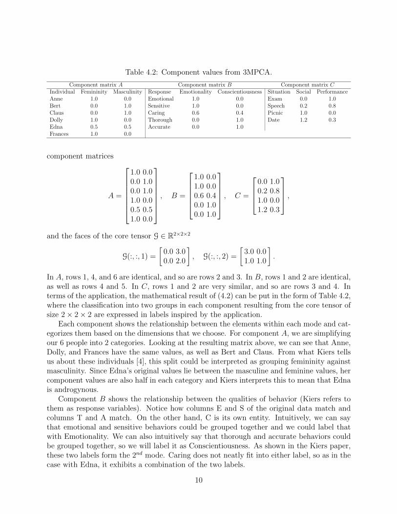
Table 4.2: Component values from 3MPCA.

Component matrix A Component matrix B Component matrix CIndividual Femininity Masculinity Response Emotionality Conscientiousness Situation Social PerformanceAnne 1.0 0.0 Emotional 1.0 0.0 Exam 0.0 1.0Bert 0.0 1.0 Sensitive 1.0 0.0 Speech 0.2 0.8Claus 0.0 1.0 Caring 0.6 0.4 Picnic 1.0 0.0Dolly 1.0 0.0 Thorough 0.0 1.0 Date 1.2 0.3Edna 0.5 0.5 Accurate 0.0 1.0Frances 1.0 0.0

component matrices

A =

1.0 0.00.0 1.00.0 1.01.0 0.00.5 0.51.0 0.0

, B =

1.0 0.01.0 0.00.6 0.40.0 1.00.0 1.0

, C =

0.0 1.00.2 0.81.0 0.01.2 0.3

,

and the faces of the core tensor G ∈ R2×2×2

G(:, :, 1) =

[0.0 3.00.0 2.0

], G(:, :, 2) =

[3.0 0.01.0 1.0

].

In A, rows 1, 4, and 6 are identical, and so are rows 2 and 3. In B, rows 1 and 2 are identical,as well as rows 4 and 5. In C, rows 1 and 2 are very similar, and so are rows 3 and 4. Interms of the application, the mathematical result of (4.2) can be put in the form of Table 4.2,where the classification into two groups in each component resulting from the core tensor ofsize 2× 2× 2 are expressed in labels inspired by the application.

Each component shows the relationship between the elements within each mode and cat-egorizes them based on the dimensions that we choose. For component A, we are simplifyingour 6 people into 2 categories. Looking at the resulting matrix above, we can see that Anne,Dolly, and Frances have the same values, as well as Bert and Claus. From what Kiers tellsus about these individuals [4], this split could be interpreted as grouping femininity againstmasculinity. Since Edna’s original values lie between the masculine and feminine values, hercomponent values are also half in each category and Kiers interprets this to mean that Ednais androgynous.

Component B shows the relationship between the qualities of behavior (Kiers refers tothem as response variables). Notice how columns E and S of the original data match andcolumns T and A match. On the other hand, C is its own entity. Intuitively, we can saythat emotional and sensitive behaviors could be grouped together and we could label thatwith Emotionality. We can also intuitively say that thorough and accurate behaviors couldbe grouped together, so we will label it as Conscientiousness. As shown in the Kiers paper,these two labels form the 2nd mode. Caring does not neatly fit into either label, so as in thecase with Edna, it exhibits a combination of the two labels.

10

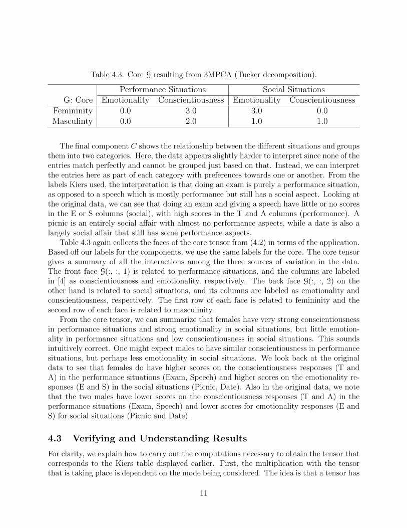
Table 4.3: Core G resulting from 3MPCA (Tucker decomposition).

Performance Situations Social SituationsG: Core Emotionality Conscientiousness Emotionality Conscientiousness

Femininity 0.0 3.0 3.0 0.0Masculinty 0.0 2.0 1.0 1.0

The final component C shows the relationship between the different situations and groupsthem into two categories. Here, the data appears slightly harder to interpret since none of theentries match perfectly and cannot be grouped just based on that. Instead, we can interpretthe entries here as part of each category with preferences towards one or another. From thelabels Kiers used, the interpretation is that doing an exam is purely a performance situation,as opposed to a speech which is mostly performance but still has a social aspect. Looking atthe original data, we can see that doing an exam and giving a speech have little or no scoresin the E or S columns (social), with high scores in the T and A columns (performance). Apicnic is an entirely social affair with almost no performance aspects, while a date is also alargely social affair that still has some performance aspects.

Table 4.3 again collects the faces of the core tensor from (4.2) in terms of the application.Based off our labels for the components, we use the same labels for the core. The core tensorgives a summary of all the interactions among the three sources of variation in the data.The front face G(:, :, 1) is related to performance situations, and the columns are labeledin [4] as conscientiousness and emotionality, respectively. The back face G(:, :, 2) on theother hand is related to social situations, and its columns are labeled as emotionality andconscientiousness, respectively. The first row of each face is related to femininity and thesecond row of each face is related to masculinity.

From the core tensor, we can summarize that females have very strong conscientiousnessin performance situations and strong emotionality in social situations, but little emotion-ality in performance situations and low conscientiousness in social situations. This soundsintuitively correct. One might expect males to have similar conscientiousness in performancesituations, but perhaps less emotionality in social situations. We look back at the originaldata to see that females do have higher scores on the conscientiousness responses (T andA) in the performance situations (Exam, Speech) and higher scores on the emotionality re-sponses (E and S) in the social situations (Picnic, Date). Also in the original data, we notethat the two males have lower scores on the conscientiousness responses (T and A) in theperformance situations (Exam, Speech) and lower scores for emotionality responses (E andS) for social situations (Picnic and Date).

4.3 Verifying and Understanding Results

For clarity, we explain how to carry out the computations necessary to obtain the tensor thatcorresponds to the Kiers table displayed earlier. First, the multiplication with the tensorthat is taking place is dependent on the mode being considered. The idea is that a tensor has

11

Figure 4.1: Unfolding of mode-3 fibers.

3 dimensions, or modes, and subscripts indicate the mode of multiplication considered whentaking the product with the factor matrices. For instance, mode-3 multiplication satisfies

Y = G×3 C ⇐⇒ Y(3) = CG(3)

where C ∈ RK×R, the G(3) ∈ RR×PQ, and Y(3) ∈ RK×PQ are mode-3 unfoldings of G ∈RP×Q×R and Y ∈ RP×Q×K . Hence, carrying out the mode-3 multiplication corresponds tounfolding or matricizing G and multiplying by C on the left (assuming the dimensions matchfor the product to be defined). Intuitively, unfolding a 3-way tensor G means to consider thefibers (that is, the columns, rows, or tubes) of a certain mode and making such fibers thecolumns of Gn (see Figure 2.2 for clarification of fibers). One can visualize this unfolding astaking the tube fibers, rotating them so as to make them columns, and then lining them upsequentially to obtain columns that form the tensor as a matrix; as presented in Figure 4.1.Thus, recall that the third component matrix in the decomposition mentioned in this sectionis

C =

1.0 0.00.8 0.20.0 1.00.3 1.2

and that the displayed frontal slices of core tensor G are

G(:, :, 1) =

[0.0 3.00.0 2.0

], G(:, :, 2) =

[3.0 0.01.0 1.0

].

Since the mode-3 unfolding means we make the tube fibers of G into columns of the unfoldedmatrix G(3), then tube fibers can be thought of as columns going into the page (towards theother slices), so that we get

G(3) =

[0.0 3.0 0.0 2.03.0 0.0 1.0 1.0

]

12

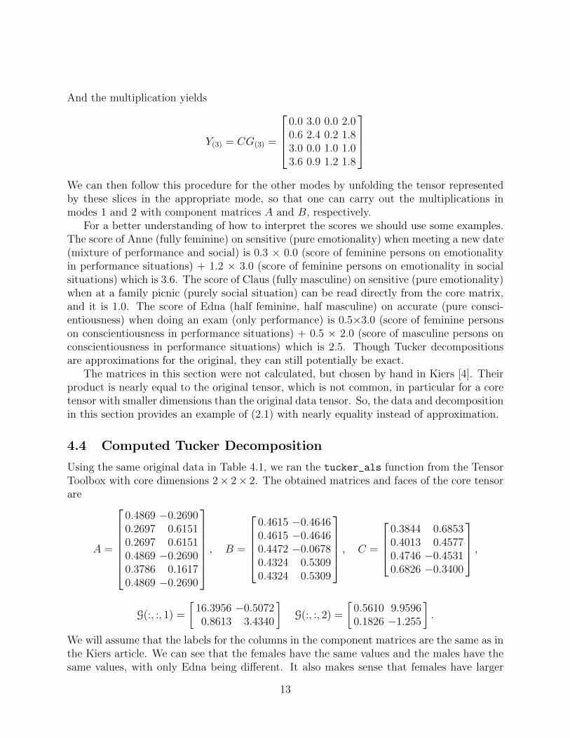
And the multiplication yields

Y(3) = CG(3) =

0.0 3.0 0.0 2.00.6 2.4 0.2 1.83.0 0.0 1.0 1.03.6 0.9 1.2 1.8

We can then follow this procedure for the other modes by unfolding the tensor representedby these slices in the appropriate mode, so that one can carry out the multiplications inmodes 1 and 2 with component matrices A and B, respectively.

For a better understanding of how to interpret the scores we should use some examples.The score of Anne (fully feminine) on sensitive (pure emotionality) when meeting a new date(mixture of performance and social) is 0.3 × 0.0 (score of feminine persons on emotionalityin performance situations) + 1.2 × 3.0 (score of feminine persons on emotionality in socialsituations) which is 3.6. The score of Claus (fully masculine) on sensitive (pure emotionality)when at a family picnic (purely social situation) can be read directly from the core matrix,and it is 1.0. The score of Edna (half feminine, half masculine) on accurate (pure consci-entiousness) when doing an exam (only performance) is 0.5×3.0 (score of feminine personson conscientiousness in performance situations) + 0.5 × 2.0 (score of masculine persons onconscientiousness in performance situations) which is 2.5. Though Tucker decompositionsare approximations for the original, they can still potentially be exact.

The matrices in this section were not calculated, but chosen by hand in Kiers [4]. Theirproduct is nearly equal to the original tensor, which is not common, in particular for a coretensor with smaller dimensions than the original data tensor. So, the data and decompositionin this section provides an example of (2.1) with nearly equality instead of approximation.

4.4 Computed Tucker Decomposition

Using the same original data in Table 4.1, we ran the tucker_als function from the TensorToolbox with core dimensions 2× 2× 2. The obtained matrices and faces of the core tensorare

A =

0.4869 −0.26900.2697 0.61510.2697 0.61510.4869 −0.26900.3786 0.16170.4869 −0.2690

, B =

0.4615 −0.46460.4615 −0.46460.4472 −0.06780.4324 0.53090.4324 0.5309

, C =

0.3844 0.68530.4013 0.45770.4746 −0.45310.6826 −0.3400

,

G(:, :, 1) =

[16.3956 −0.50720.8613 3.4340

]G(:, :, 2) =

[0.5610 9.95960.1826 −1.255

].

We will assume that the labels for the columns in the component matrices are the same as inthe Kiers article. We can see that the females have the same values and the males have thesame values, with only Edna being different. It also makes sense that females have larger

13

values of femininity as opposed to masculinity (note the negative signs for masculinity),though it’s surprising that the males have much higher values of masculinity, but still somefemininity (note the positive signs). We can see something similar with the grouping of theresponse variables. From this, we might also interpret that an exam is mostly a performancesituation, with still some social aspects which sounds unintuitive.

Looking at the core tensor, we decided to reverse the labeling for the columns in order topreserve the interpretation under the assumption that the high value of 16.3956 correspondsto what should be the high value for female conscientiousness in performance situations.Just as in the example from Kiers, we can summarize that females have very strong con-scientiousness in performance situations and strong emotionality in social situations, butlittle emotionality in performance situations and low conscientiousness in social situations,which is similar to results in the Kiers article. One might also expect males to have similarconscientiousness in performance situations, but perhaps less emotionality in social situa-tions. Surprisingly, this decomposition tells us that males have a fairly strong emotionalitytowards performance situations, with little response at all towards social scenarios. Lookingback at the data, we can see that females do indeed have higher scores on the conscien-tiousness responses (T and A) and higher scores on the emotionality responses (E and S) inthe performance situations (Exam, Speech) and social situations (Picnic, Date) respectively.While the two males do show low scores on everything in the social situations, they don’tshow comparatively higher emotionality on the performance situations. This iterative pro-cess leads to a different interpretation than the Kiers article and is a potential nuance forfurther study.

4.5 Other Core Tensor Dimensions

Since the Tucker decomposition allows us to specify the dimensions we want to use, we arenot limited to cube cores (such as 2× 2× 2). Say, for instance, we wanted to see if using 3classifications for people beyond male and female would be a better fit to represent Edna asopposed to being a composite between male and female. We would specify the core tensor tobe 3×2×2, and the first component should have 3 columns. The individuals who are purelyone or the other should have the same if not very similar values in their original columns,while Edna should undergo a drastic change in both of the 2 original columns now that Ednais freed from the constraint of 2 classifications.

Comparing the A matrix from Section 4.4 to Table 4.4, we see our original columns foreveryone except Edna are the same, and everyone has negative values in the third column,except for Edna in this instance. If the Kiers article did something similar, we could expectthe third column to have a 1.0 for Edna with 0.0 in masculinity and femininity. A similarcomponent matrix could be generated for the response variables. Since Caring has a differentvalue from all other response variables, it may have a strong correlation to the third categoryif we specified our core to have dimensions of 2× 3× 2. It should be noted that having coredimensions very close to the original data’s dimensions serve little purpose since the goalis to shrink the original data to a size that can be summarized. Having any of the coredimensions as 1 would also be unproductive, since we would not be categorizing the modes

14

Table 4.4: Component matrix A for the Tucker decomposition with 3 categories.

Component matrix AIndividual Femininity Masculinty OtherAnne 0.4869 −0.2690 −0.1546Bert 0.2697 0.6151 −0.2211Claus 0.2697 0.6151 −0.2211Dolly 0.4869 −0.2690 −0.1546Edna 0.3786 0.1615 0.9114Frances 0.4869 −0.2690 −0.1546

or showing any useful numbers for comparison.

5 Practical Application of Tensor Decomposition

We now look at a larger data set that still has the same structure as the illustrative examplein Section 4. This data set is one of many available through the Three-Mode Company [7],a website devoted to providing three-mode data sets to motivate the use of three-modedata analysis. We discuss a couple ways in which one can make use of the results of thedecomposition to obtain meaningful information.

5.1 Dutch Children Psychological Experiment

The data set consists of results from a Dutch psychological experiment involving:

• I = 326 children who exhibited

• J = 5 behaviors — Proximity Seeking (PS), Contact Maintaining (CM), Resistance(R), Avoidance (AV), Distance Interaction (DI) — in

• K = 2 stressful situations where the children were put in a room with a stranger andthe mother was later brought back.

Hence, the data can be represented in the form of a 3-way tensor X ∈ R326×5×2. A scorebetween 1 and 7 is given to each child to rate their behavior in each of the 5 categoricalscales. Data collected for the first 5 children in situation 1 is displayed in Table 5.1 forexample.

5.2 Applying Tucker decompoisition

We compute a Tucker decomposition using tucker als with a requested core tensor size of2× 2× 2. The 2 for the first mode attempts to split the children in 2 groups. For the secondmode, the 2 attempts to place the more closely related behaviors together. For the third

15

Table 5.1: First five rows of Dutch data.

Individual PS CM R AV DI1 3 2 1 2 72 6 7 1 1 13 1 2 1 2 74 7 7 7 1 15 6 4 4 1 1

mode, we pick it as a default since there are 2 situations. Thus, we obtain core G ∈ R2×2×2,and component matrices A ∈ R326×2, B ∈ R5×2, and C ∈ R2×2.

A =

0.0476 −0.06630.0571 0.0811

......

0.0556 −0.02360.0547 −0.0455

, B =

0.5444 −0.37050.4363 −0.50900.3391 −0.13130.3919 0.31240.4947 0.6992

, C =

[0.7342 0.6789−0.6778 0.7342

],

G(:, :, 1) =

[0.3376 16.3568−1.7602 0.7655

]G(:, :, 2) =

[178.6889 −0.6780−0.0978 −80.4707

]Oftentimes, the interest in psychological experiments is to understand behavioral pat-

terns. With this motivation, we restrict our attention to the B matrix because it correspondsto the 5 response variables:

B =

0.5444 −0.37050.4363 −0.50900.3391 −0.13130.3919 0.31240.4947 0.6992

Proximity Seeking

Contact MaintainingResistanceAvoidance

Distance Interaction

By sign and magnitude, the second column of B noticeably groups the first three behaviorsof Proximity Seeking, Contact Maintaining, and Resistance and the last two behaviors ofAvoidance and Distance Interaction.

We project the first 5 children’s data onto the second column of B. In other words, wetake the dot product of each row of the children’s data with the second column of B:

X(1 : 5, :, 1)B(:, 2) =

3 2 1 2 76 7 1 1 11 2 1 2 77 7 7 1 16 4 4 1 1

−0.3705−0.5090−0.1313

0.31240.6992

=

3.2583−4.0955

3.9993−6.0638−3.7725

.

Negative values correspond to the extent to which behaviors of Proximity Seeking and/orContact Maintaining are present. Positive values correspond to the extent to which behaviors

16

of Avoidance and/or Distance Interaction are present. This projection helps summarizeinformation about the behavior of each child in situation 1.

The Tensor Toolbox allows us to request different tensor core sizes. For further explo-ration, we compute a Tucker decomposition by requesting a core tensor of size 2 × 3 × 2,which results in

A =

0.0476 −0.06670.0570 0.0807

......

0.0552 −0.02400.0546 −0.0458

, B =

0.5444 −0.3706 0.64700.4363 −0.5084 −0.55730.3391 −0.1316 −0.31010.3919 0.3111 0.32380.4947 0.7001 −0.2643

, C =

[0.7342 0.6790−0.6790 0.7342

]

G(:, :, 1) =

[0.3369 16.3405 4.6376−1.7663 0.7502 1.3683

], G(:, :, 2) =

[178.6895 −0.0863 0.0055−0.1397 −80.4702 0.9545

]We also compute a Tucker decomposition for a core tensor of size 2× 4× 2, which gives

A =

0.0476 −0.06630.0570 0.0809

......

0.0552 −0.02420.0546 −0.0456

, B =

0.5444 −0.3713 0.6499 −0.00870.4363 −0.5086 −0.5581 −0.45550.3391 −0.1305 −0.3113 0.87600.3919 0.3128 0.3178 −0.04830.4947 0.6990 −0.2612 −0.1509

, C =

[0.7342 0.6789−0.6789 0.7342

]

G(:, :, 1) =

[0.3446 16.3399 4.6349 −0.4621−1.7529 0.7657 1.3615 1.6279

], G(:, :, 2) =

[178.6896 −0.0853 0.0051 0.0168−0.1362 −80.4694 0.9541 −0.0784

]In this instance, the first and second columns of B do not drastically change across the

different sizes of the core tensor.It is important to note at this point that we have performed a similar decomposition

on two different sets of data, but used them for different methods of interpretation. Withthe Kiers article, the decomposition was used to show how all of the components relatedto each other and is an illustrative example on how to label the columns given that theproperties of the individuals are known. For the Dutch experiment, we chose to only focuson the B matrix that corresponded to the response variables. Due to the similarity of signand magnitude of the first column in B, we chose to focus on the second column. We haveextended the analysis done with Tucker by projecting the rows of the original data ontothe second column of the second component matrix B. Doing this allowed us to provide asummary of the children’s behavioral tendencies. How one chooses to analyze and interpretthe results depends on the data that is being used as well as what the user wants to look for.

Acknowledgments

These results were obtained as part of the REU Site: Interdisciplinary Program in High Per-formance Computing (hpcreu.umbc.edu) in the Department of Mathematics and Statisticsat the University of Maryland, Baltimore County (UMBC) in Summer 2016. This program

17

is funded by the National Science Foundation (NSF), the National Security Agency (NSA),and the Department of Defense (DOD), with additional support from UMBC, the Depart-ment of Mathematics and Statistics, the Center for Interdisciplinary Research and Consulting(CIRC), and the UMBC High Performance Computing Facility (HPCF). HPCF is supportedby the U.S. National Science Foundation through the MRI program (grant nos. CNS–0821258and CNS–1228778) and the SCREMS program (grant no. DMS–0821311), with additionalsubstantial support from UMBC. Co-author Darren Stevens II was supported, in part, bythe UMBC National Security Agency (NSA) Scholars Program through a contract with theNSA. Graduate assistant Jonathan Graf was supported by UMBC.

References

[1] E. Acar, D. M. Dunlavy, and T. G. Kolda. Link prediction on evolving data usingmatrix and tensor factorizations. In 2009 IEEE International Conference on Data MiningWorkshops, pages 262–269, Dec. 2009.

[2] D. Fitzgerald, E. Coyle, and M. Cranitch. Using tensor factorisation models to separatedrums from polyphonic music. In Proceedings of the International Conference on DigitalAudio Effects (DAFX09), 2009.

[3] U. Kang, Evangelos Papalexakis, Abhay Harpale, and Christos Faloutsos. Gigatensor:Scaling tensor analysis up by 100 times — algorithms and discoveries. In Proceedingsof the 18th ACM SIGKDD International Conference on Knowledge Discovery and DataMining, KDD ’12, pages 316–324. ACM, 2012.

[4] Henk A. L. Kiers and Iven Van Mechelen. Three-way component analysis: Principlesand illustrative application. Psychological Methods, 6:84–110, 2001.

[5] T. G. Kolda and J. Sun. Scalable tensor decompositions for multi-aspect data mining. In2008 Eighth IEEE International Conference on Data Mining, pages 363–372, Dec. 2008.

[6] Tamara G. Kolda and Brett W. Bader. Tensor decompositions and applications. SIAMReview, 51(3):455–500, 2009.

[7] Pieter M. Kroonenberg. The three-mode company. http://three-mode.leidenuniv.

nl. Accessed September 12, 2016.

[8] Evangelos E. Papalexakis, U. Kang, Christos Faloutsos, Nicholas D. Sidiropoulos, andAbhay Harpale. Large scale tensor decompositions: Algorithmic developments and ap-plications. IEEE Data Engineering Bulletin, 36(3):59–66, 2013.

18